A GKP qubit protected by dissipation in a high-impedance superconducting circuit driven by a microwave frequency comb

Abstract

We propose a novel approach to generate, protect and control GKP qubits. It employs a microwave frequency comb parametrically modulating a Josephson circuit to enforce a dissipative dynamics of a high impedance circuit mode, autonomously stabilizing the finite-energy GKP code. The encoded GKP qubit is robustly protected against all dominant decoherence channels plaguing superconducting circuits but quasi-particle poisoning. In particular, noise from ancillary modes leveraged for dissipation engineering does not propagate at the logical level. In a state-of-the-art experimental setup, we estimate that the encoded qubit lifetime could extend two orders of magnitude beyond the break-even point, with substantial margin for improvement through progress in fabrication and control electronics. Qubit initialization, readout and control via Clifford gates can be performed while maintaining the code stabilization, paving the way toward the assembly of GKP qubits in a fault-tolerant quantum computing architecture.

[maintext] [maintext]l1

Contents

I Introduction

Despite considerable progress realized over the past decades in better isolating quantum systems from their fluctuating environment, noise levels in all explored physical platforms remain far too high to run useful quantum algorithms. Quantum error correction (QEC) would overcome this roadblock by encoding a logical qubit in a high-dimensional physical system and correcting noise-induced evolutions before they accumulate and lead to logical flips. In stabilizer codes, such errors are unambiguously revealed by measuring stabilizer operators [1], which commute with the logical Pauli operators and thus do not perturb the encoded qubit. A central assumption behind QEC is that a physical system only interacts with its noisy environment via low-weight operators. For instance, in discrete variable codes such as the toric code [2], the surface code [3, 4] or the color code [5], the logical qubit is encoded in a collection of physical two-level systems devoid of many-body interactions. In bosonic codes such as the GKP code [6, 7], the Schrödinger cat code [8, 9] and the binomial code [10, 11], the qubit is encoded in a quantum oscillator whose interactions, denoted here as low-weight interactions, involve a small number of photons . Under these assumptions, noise does not directly induce logical flips between well-chosen code states. Specifically, codes are constructed such that several two-level systems should flip in order to induce a logical flip in the former case, and that a multi-photonic transition should occur in the latter case. Admittedly, logical flips may occur indirectly as low-weight interactions can generate a high-weight evolution operator, but this evolution takes time and is correctable provided that QEC is performed sufficiently fast.

The aforementioned bosonic codes are appealing for their moderate hardware overhead, but a paradox emerges in their operation: some of their stabilizers are high-weight operators that do not appear naturally in the system interactions. A common strategy to measure these stabilizers is to map their value to an ancilla system via an evolution operator generated from a low-weight interaction. It was successfully employed to stabilize cat codes [13], binomial codes [11] and the GKP code [14], but results in the opening of uncorrectable error channels. As illustrated in Fig. 1a in the case of the GKP code, while the interaction is carefully timed so that the overall evolution operator leaves code states unaffected in the absence of noise, ancilla errors during the interaction propagate as uncontrolled long shifts of the target system, triggering logical flips. Partial QEC of the ancilla [15] or error mitigation [16, 17, 18] was proposed to suppress this advert effect, but the robust implementation of these ideas is a major experimental challenge [19]. An alternative strategy, more robust but experimentally more demanding, consists in engineering high-weight interactions so that the target system only interacts with the ancilla via its stabilizer operators. In this configuration, ancilla noise propagates to the target system as an evolution operator generated by the stabilizers only, which leaves the logical qubit unaffected (see Fig. 1b).

Focusing on the GKP code, the two stabilizers are commuting trigonometric functions of the oscillator position and momentum (high-weight operators), which generate discrete translations along a grid in phase-space. The phase of these so-called modular operators [20, 21, 22, 23] reveals spurious small shifts of the oscillator state in phase-space while supporting no information on the encoded qubit state. Most proposals [24, 25, 26, 27, 28, 29] and all experimental demonstrations [14, 30, 31] of GKP state preparation and error-correction are based on variants of phase-estimation [32, 33] of the stabilizers. Phase-estimation falls into the first category of stabilizer measurement strategies described above, and therefore leaves the target system open to uncorrectable error channels. In this paper, we consider the second, more robust strategy and aim at engineering high-weight interactions involving only the two modular stabilizers. The state of the oscillator would then only hop along the GKP code lattice in phase-space (see Fig. 1b for schematic hopping along one phase-space quadrature). But how can we engineer a coupling Hamiltonian involving two modular operators?

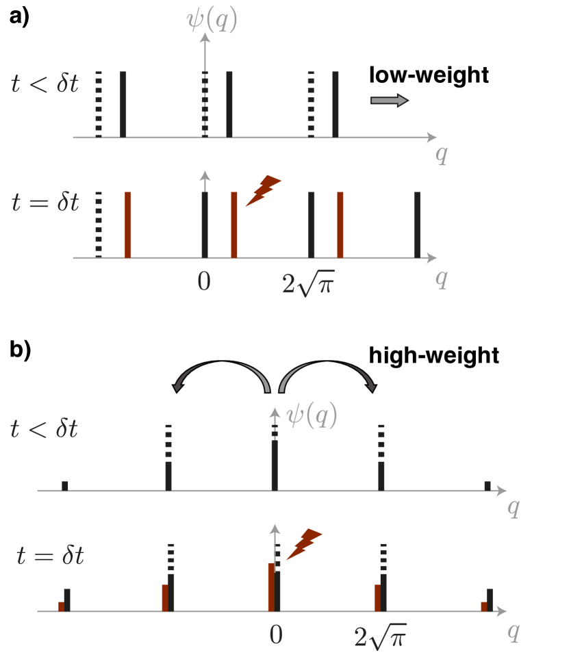
Figure 1: a) Low-weight interactions. ${\bf H}=-g{\bf p}{\bf B}$ is an example of low-weight Hamiltonian employed in recent experiments stabilizing the GKP code. It entails a continuous displacement of a GKP state along the $q$ quadrature of an oscillator (plain black lines, initial state represented by dashed black lines), conditioned on an ancillary mode observable $B$. The interaction duration $\delta t$ is chosen such that the state is displaced by one period of the square GKP lattice after the evolution. However, if noise modifies the value of $B$ during the interaction (red lightning), the final target state is shifted (red lines) and the GKP qubit may be flipped (see Sec. II). b) High-weight interactions. ${\bf H}=-g\mathrm{cos}(2\sqrt{\pi}{\bf p}){\bf B}$ is a high-weight (modular) Hamiltonian that entails a hopping dynamics along the GKP lattice. If noise modifies the value of $B$ during the interaction, the relative weights of the final state peaks may be affected but not their positions, so that no logical flip may occur.

An isolated Josephson junction behaves as an inductive element whose dynamics is governed by a modular flux operator. However, in most circuitQED experiments [34], the junction is shunted by a low-impedance circuitry, so that it effectively acts on the circuit modes as a weakly non-linear, low-weight, operator. In contrast, connecting the junction to a circuit whose impedance exceeds the quantum of resistance—a regime recently attained in circuitQED—reveals its truly modular nature [35]. Unfortunately, experimental implementations of the dual coherent phase-slip element, whose dynamics is governed by a modular charge operator [36] are not yet coherent enough for practical use [37]. Moreover, the doubly modular Hamiltonian implemented by the association of these two elements would only stabilize a single GKP state and not a two-dimensional code manifold [38]. The $0-\pi$ qubit [39, 40] is an elementary protected circuit that would circumvent these two pitfalls. In this circuit, an effective coherent phase-slip behavior emerges in the low energy dynamics of an ultra-high impedance fluxonium mode [41, 42]. When appropriately coupled to a transmon mode [43], the quasi-degenerate ground manifold is spanned by a pair of two-mode GKP states [44]. However, fully fledged GKP states are only obtained in an extreme parameter regime currently out of reach [40]. Recently, Rymarz et al. [45] proposed an alternative approach to offset the lack of a phase-slip element. Building on an idea suggested in the original GKP proposal [6], they realized that two Josephson junctions bridged by a high-impedance gyrator would implement a doubly modular Hamiltonian stabilizing quasi-degenerate GKP states. However, existing gyrators are either far too limited in impedance and bandwidth [46, 47, 48] or rely on strong magnetic fields incompatible with superconducting circuits [49].

In this paper, we propose to engineer a true doubly modular Hamiltonian in the rotating frame of a state-of-the-art Josephson circuit. The method, similar to the twirling-based engineering introduced in Ref. [50], is schematically represented in Fig. 2. A Josephson junction allows the coherent tunneling of Cooper pairs across a high-impedance circuit mode, translating its state by $\pm 2e$ along the charge axis of phase-space. Modulating the tunneling rate with fast pulses, we ensure that such translations occur every quarter period of the target mode only, and let the state rotate freely in phase-space in-between pulses. As a result, the state evolves in discrete steps on a square grid, which matches the GKP code lattice for the proper choice of target mode impedance. We combine this novel approach with dissipation-engineering techniques successfully employed to stabilize Schrödinger cat states [13, 51], so that the target oscillator autonomously stabilizes in the GKP code manifold. Mathematical analysis and numerical simulations show that this strategy can enhance the logical qubit coherence far beyond that of the underlying circuit. Moreover, we describe how to control encoded qubits with fault-tolerant Clifford gates, paving the way toward a high-fidelity quantum computing architecture based on GKP qubits.

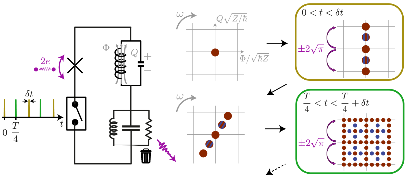
Figure 2: Schematic representation of modular dissipation engineering. A switch controls the coherent tunneling of Cooper pairs (charge $2e$) across a Josephson junction placed in parallel of a two-mode circuit. The target mode (top) has a high impedance $Z$ such that, in normalized phase-space coordinates, tunneling events translate its state by $\pm 2\sqrt{\pi}$ along the charge axis. The switch is controlled with a train of sharp pulses (duration $\delta t$) activating tunneling every quarter of a period $T$ of the target oscillator. In between pulses, the oscillator state rotates freely in phase-space at $\omega=2\pi/T$. Overall, the target mode dynamics is generated by discrete shifts along a square grid matching the GKP lattice (gray grid with period $2\sqrt{\pi}$ overlaid with Wigner diagrams of the oscillator state). A lower impedance ancillary mode (bottom), also driven by Cooper pair tunneling, dissipates excitations into a cold load (purple wriggled arrow) to ensure that the target mode dynamics is irreversible, autonomously stabilizing the GKP code.

The paper is organized as follows. In Sec. II, we review the properties of idealized GKP states and their realistic, finite-energy counterparts. In Sec. III, we propose a dissipative dynamics based on four modular Lindblad operators stabilizing the finite-energy GKP code, and benchmark its error-correction performances against the dominant decoherence channels plaguing superconducting resonators. In Sec. IV, we show how to engineer a doubly modular Hamiltonian in a high-impedance, parametrically driven Josephson circuit. In Sec. V, we combine this method with reservoir engineering techniques to obtain the target modular dissipation. In Sec.VI, we briefly discuss the impact of various noise processes and that of circuit fabrication constraints and disorder. We refer the reader to the Supplemental materials for a more detailed analysis. Finally, in Sec. VII we sketch how to fault-tolerantly control encoded GKP qubits with Clifford gates.

II The GKP code

GKP introduced coding grid states as superpositions of periodically spaced position states of a quantum oscillator. For simplicity’s sake, we consider throughout this paper square grid states—see Supplemental Materials for generalization to hexagonal grid states—defined as

$$\begin{split}&|+Z_{\infty}\rangle=\sum_{n\in\mathbb{Z}}|n\eta\rangle_{q}=\sum_{n\in\mathbb{Z}}|\frac{2\pi n}{\eta}\rangle_{p}\\ &|-Z_{\infty}\rangle=\sum_{n\in\mathbb{Z}}|(n+\tfrac{1}{2})\eta\rangle_{q}=\sum_{n\in\mathbb{Z}}(-1)^{n}|\frac{2\pi n}{\eta}\rangle_{p}\end{split}$$ (1)

where $\eta=2\sqrt{\pi}$ and $|r\rangle_{q}$ (respectively $|r\rangle_{p}$) denotes an eigenstate with eigenvalue $r$ of the oscillator normalized position ${\bf q}=({\bf a}+{\bf a^{\dagger}})/\sqrt{2}$ (respectively momentum ${\bf p}=({\bf a}-{\bf a^{\dagger}})/(i\sqrt{2})$), ${\bf a}$ being the annihilation operator. One can show that any pair of orthogonal logical states have distant support in phase-space, providing the code robustness against position and momentum shift errors. Since the evolution of an oscillator quasi-probability distribution in phase-space is diffusive under the action of noise coupling via low-weight operators [52], this robustness extends to all dominant error channels in superconducting resonators.

Error-syndromes are extracted by measuring the phase of the code stabilizers ${\bf S}_{q}=e^{i\eta{\bf q}}$ and ${\bf S}_{p}=e^{-i\eta{\bf p}}$, which is 1 inside the code manifold. Given that the logical qubit can be perfectly decoded as long as the oscillator is not shifted by more than $\sqrt{\pi}/2$, we define generalized Pauli operators ${\bf Z}=\mathrm{Sgn}\big{(}\mathrm{cos}(\frac{\eta}{2}{\bf q})\big{)}$, ${\bf X}=\mathrm{Sgn}\big{(}\mathrm{cos}(\frac{\eta}{2}{\bf p})\big{)}$ and ${\bf Y}=i{\bf Z}{\bf X}$. Here, the superoperator $\mathrm{Sgn}(\cdot)$ denotes the sign of a real-valued operator and is applied to the logical operators introduced by GKP. With our definition, ${\bf X}$, ${\bf Y}$ and ${\bf Z}$ respect the Pauli algebra composition rules throughout the oscillator Hilbert space and coincide with the logical qubit Pauli operators inside the code manifold. Intuitively, the expectation values of these operators are the qubit Bloch sphere coordinates found when decoding the outcomes of homodyne detections, respectively along ${\bf p}$, $({\bf q}+{\bf p})$ and ${\bf q}$. The qubit they define can remain pure whilst the oscillator state is not. Moreover, we verify that they commute with the stabilizers, which can thus be measured without perturbing the encoded qubit. More generally, a noisy environment coupling to the oscillator via the stabilizer operators does not induce logical errors: this is the core idea guiding our approach.

Even though infinitely squeezed grid states are physically unrealistic, GKP suggested that these desirable features would be retained for the normalized, finitely squeezed states $|\pm Z_{\Delta}\rangle={\bf E}_{\Delta}|\pm Z_{\infty}\rangle$ where ${\bf E}_{\Delta}=e^{-\Delta{\bf a^{\dagger}}{\bf a}}$ with $\Delta\ll 1$. Analogously to the infinitely squeezed case, these two states are $+1$-eigenstates of the commuting, normalized, stabilizers ${\bf S}_{q}^{\Delta}={\bf E}_{\Delta}{\bf S}_{q}{\bf E}_{\Delta}^{-1}$ and ${\bf S}_{p}^{\Delta}={\bf E}_{\Delta}{\bf S}_{p}{\bf E}_{\Delta}^{-1}$. However, they are not orthogonal since their wavefunction peaks are Gaussian with a non-zero standard deviation $\sigma=(\mathrm{tanh}(\Delta))^{\frac{1}{2}}$. Orthogonal, finite-energy logical states can be rigorously defined as their symmetric and antisymmetric superpositions, and Pauli operators for the finite-energy code can be defined therefrom. Nevertheless, in the following, we retain the encoded qubit as defined by the ${\bf X}$, ${\bf Y}$ and ${\bf Z}$ operators. Even though this definition does not allow the preparation of a pure logical state at finite energy, it is operationally relevant as these observables can be measured experimentally. Moreover, the qubit maximum purity is exponentially close to 1 as $\Delta$ approaches $0$, so that the encoded qubit is well suited for quantum information processing applications for only modest average photon number in the grid states: we find $1-(\langle{\bf X}\rangle^{2}+\langle{\bf Y}\rangle^{2}+\langle{\bf Z}\rangle^{2})^{1/2}\simeq 2\times 10^{-8}$ for a pure finite-energy code state containing $\overline{n}=10$ photons.

III Protection of GKP qubits by modular dissipation

III.1 Stabilization of the code manifold

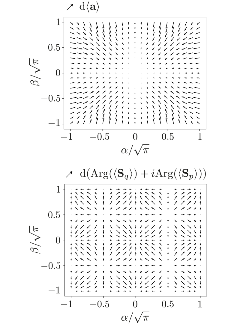
Figure 3: Modular dissipation phase portraits. For a finite-energy code state ($\mathrm{sinh}(\Delta)=0.2/\eta$) displaced by $\alpha+i\beta$ in phase-space, arrows encode the evolution of the state center of mass (top panel) and modular coordinates (bottom panel) entailed by the Lindblad operators (3) over a short time step $\mathrm{d}t\ll 1/\Gamma$. Arrows length are rescaled to arbitrary units.

In Ref. [53], it was shown that a dissipative dynamics based on four Lindblad operators derived from the two finite-energy code stabilizers and their images by a $\pi$ rotation in phase space stabilizes the code manifold. More precisely, denoting $\mathcal{D}[{\bf L}]$ the dissipator formed from an arbitrary operator ${\bf L}$ and defined by its action on the density matrix $\mathcal{D}[{\bf L}](\bm{\rho})={\bf L}\bm{\rho}{\bf L}^{\dagger}-\frac{1}{2}({\bf L}^{\dagger}{\bf L}\bm{\rho}+\bm{\rho}{\bf L}^{\dagger}{\bf L})$, the finite-energy code states are fixed points of the Lindblad equation

$$\frac{\mathrm{d}\bm{\rho}}{\mathrm{d}t}=\Gamma\sum^{3}_{k=0}\mathcal{D}[{\bf M}_{k}](\bm{\rho}),$$ (2)

where ${\bf M}_{k}={\bf R}_{\frac{k\pi}{2}}({\bf S}_{q}^{\Delta}-{\bf 1}){\bf R}^{\dagger}_{\frac{k\pi}{2}}$, ${\bf R}_{\theta}=e^{i\theta{\bf a^{\dagger}}{\bf a}}$ performs a rotation by $\theta$ in phase-space and $\Gamma$ is the dissipation rate. Indeed, the offsets by $-{\bf 1}$ ensure that each Lindblad operator cancels on the code manifold. Moreover, any initial state of the oscillator converges exponentially toward the code manifold at a rate set by $\Gamma$ and $\Delta$.

Unfortunately, the ${\bf M}_{k}$ operators are products of trigonometric and hyperbolic functions of ${\bf q}$ and ${\bf p}$, which would prove formidably challenging to engineer in an experimental system. Here, we propose to approximate them to first order in $\Delta$ by products of trigonometric and linear functions of ${\bf q}$ and ${\bf p}$ with the operators

$${\bf L}_{k}=\mathcal{A}{\bf R}_{\frac{k\pi}{2}}e^{i\eta{\bf q}}({\bf 1}-\epsilon{\bf p}){\bf R}^{\dagger}_{\frac{k\pi}{2}}-{\bf 1},$$ (3)

where $\epsilon=\eta~{}\mathrm{sinh}(\Delta)$ is a small parameter and the scalar factor $\mathcal{A}=e^{-\eta\epsilon/2}$ originates from the non commutativity of ${\bf q}$ and ${\bf p}$ in the Baker-Campbell-Hausdorff formula.

In order to qualitatively apprehend the dynamics entailed by these modular Lindblad operators, we represent in Fig. 3 the evolution of a displaced code state $\bm{\rho}_{\alpha+i\beta}=e^{-i\alpha{\bf p}+i\beta{\bf q}}|+Z_{\Delta}\rangle\langle+Z_{\Delta}|e^{+i\alpha{\bf p}-i\beta{\bf q}}$ over an infinitesimal time step $\mathrm{d}t\ll 1/\Gamma$. On the top panel, arrows represent the variation of the state center of mass (vector complex coordinates proportional to $\mathrm{d}\mathrm{Tr}({\bf a}~{}\bm{\rho}_{\alpha+i\beta})$). A single attractor at the origin of phase-space pins the grid state normalizing envelope. On the bottom panel, arrows represent the variation of the state position and momentum modulo $2\pi/\eta$ (vector complex coordinates proportional to $\mathrm{d}\mathrm{Tr}(\mathrm{Arg}[{\bf S}_{q}\bm{\rho}_{\alpha+i\beta}]+i\mathrm{Arg}[{\bf S}_{p}\bm{\rho}_{\alpha+i\beta}])$). Multiple attractors appear for $\alpha,~{}\beta=0~{}\mathrm{mod}~{}2\pi/\eta$ pinning the grid peaks onto the GKP code lattice. Note that here, we employ the displaced grid state $\bm{\rho}_{\alpha+i\beta}$ as a sensitive position and momentum shift detector [54], but initializing the oscillator in a less exotic state such as a coherent state centered in $\alpha,\beta$ yields similar phase portraits, albeit smoothed by the state quadrature fluctuations. These observations hint at a convergent dynamics toward the finite-energy code manifold, irrespective of the oscillator initial state. This contrasts with the Lindblad dynamics based on only two modular dissipators introduced in Ref. [29], for which we observe dynamical instabilities [55].

Quantitatively, we show that, under this four-dissipator dynamics, the expectation values of the infinite-energy code stabilizers converge to their steady state value at a rate $\Gamma_{c}\gtrsim\mathcal{A}\epsilon\eta\Gamma$ and that the oscillator energy remains bounded [55], proving that the dynamics is indeed stable. Note that, due to the linear approximation of hyperbolic functions we made to obtain the operators (3), the state reached by the oscillator after a few $1/\Gamma_{c}$ does not strictly belong to the code manifold, but consists in a statistical mixture of shifted code states. In terms of phase-space quasiprobability distribution, this results in broader peaks for the stabilized grid states. Yet, the overlap of a peak with its neighbors remains exponentially small as $\epsilon$ decreases, so that high-purity encoded states can still be prepared, and population leakage between two orthogonal logical states occurs on a timescale much longer than $1/\Gamma_{c}$. Quantitatively, we show that when $\epsilon\ll 1$, the generalized Pauli operators ${\bf X}$ and ${\bf Z}$ decay at a rate $\Gamma^{0}_{L}=\frac{4}{\pi}\mathcal{A}\epsilon\eta\Gamma e^{-\frac{4}{\mathcal{A}\epsilon\eta}}$, while ${\bf Y}$ decays twice faster, as expected for the square GKP code.

III.2 Autonomous quantum error correction

Given that the confinement strength onto the code manifold $\Gamma_{c}$ and the residual error rate $\Gamma^{0}_{L}$ both depend on $\epsilon$, this value needs to be optimized when correcting for errors induced by intrinsic noise channels. Indeed, $\epsilon$ should not be too small for the modular dissipation to cancel efficiently the stochastic shifts induced by a low-weight noise process, but not too large for the grid state peaks to be well resolved. In the case of quadrature noise entering the Lindblad dynamics as two spurious dissipators $\mathcal{D}[\sqrt{\kappa}{\bf q}]$ and $\mathcal{D}[\sqrt{\kappa}{\bf p}]$, we show that, in the limit of weak intrinsic dissipation $\kappa\ll\Gamma_{c}$, the decay rate of the generalized Pauli operators ${\bf X}$ and ${\bf Z}$ reads $\Gamma_{L}=\frac{4}{\pi}\mathcal{A}\epsilon\eta\Gamma e^{-4/(\mathcal{A}\tilde{\epsilon}\eta)}$, where $\tilde{\epsilon}=\epsilon+\frac{\kappa}{2\mathcal{A}^{2}\epsilon\Gamma}$ [55]. The minimum flip rate is obtained for $\epsilon\simeq(\frac{\kappa}{2\mathcal{A}^{2}\Gamma})^{\frac{1}{2}}$ and reads $\Gamma_{L}\simeq\frac{4\eta}{\pi}(\frac{\kappa\Gamma}{2})^{\frac{1}{2}}e^{-(\frac{8\Gamma}{\eta^{2}\kappa})^{\frac{1}{2}}}$. This exponential scaling ensures that logical errors can be heavily suppressed for a modest ratio $\Gamma/\kappa$, as illustrated by Fig. 4a. There, we represent the decay rate of the generalized Pauli operators ${\bf X}$ and ${\bf Z}$ extracted by spectral analysis of the Lindblad superoperator (dashed lines), in quantitative agreement with a full Lindblad master equation simulation (dots). The latter is computationally much more costly but proves necessary to investigate more realistic noise models for which no simulation shortcut was found. In particular, we verify numerically that errors entailed by single-photon dissipation, pure dephasing and a Kerr Hamiltonian perturbation all appear to be exponentially suppressed when increasing the modular dissipation rate (see Fig. 4b-d). The logical error rates induced by the two latter processes—entering the Lindblad equation via fourth order polynomials in ${\bf q}$ and ${\bf p}$—are qualitatively captured by a mean-field approximation which boils down to quadrature noise scaled up by the grid states mean photon number $\overline{n}=\eta/(2\epsilon)$ (dashed gray lines in Fig. 4c-d). These numerical considerations support the intuition that modular dissipation can suppress errors induced by arbitrary finite-weight noise channels, albeit with degraded performances when considering higher-weight processes. In the limit of infinite-weight noise processes, i.e. modular noise channels, errors are not corrected.

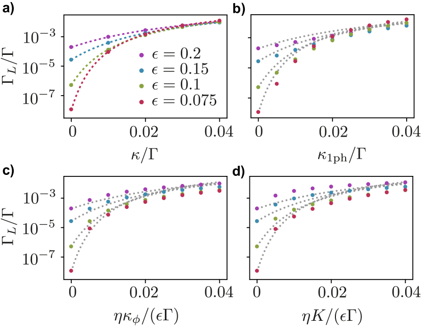
Figure 4: GKP qubit protection by modular dissipation. The decay rate $\Gamma_{L}$ of the Pauli operators ${\bf Z}$ and ${\bf X}$ is extracted from numerical simulations (dots) when varying the strength of some intrinsic noise channel relative to the modular dissipation rate $\Gamma$. For all low-weight noise channels considered, errors appear to be exponentially suppressed in the weak noise limit. a) Quadrature noise modeled by two Lindblad operators $\sqrt{\kappa}{\bf q}$ and $\sqrt{\kappa}{\bf p}$. Dashed lines are predictions by spectral analysis of the Lindblad superoperator [55]. b) Single-photon dissipation modeled by a Lindblad operator $\sqrt{\kappa_{1\mathrm{ph}}}{\bf a}$. c) Pure dephasing modeled by a Lindblad operator $\sqrt{\kappa_{\phi}}{\bf a}^{\dagger}{\bf a}$. d) Kerr Hamiltonian perturbation of the form $\frac{K}{2}({\bf a}^{\dagger}{\bf a})^{2}$. For (c-d), note the rescaling of the x-axis by $\eta/\epsilon=2\overline{n}$. For (b-d), dashed gray lines reproduce the dashed colored lines in (a), un-rescaled, for comparison.

IV Modular Hamiltonian engineering in a Josephson circuit

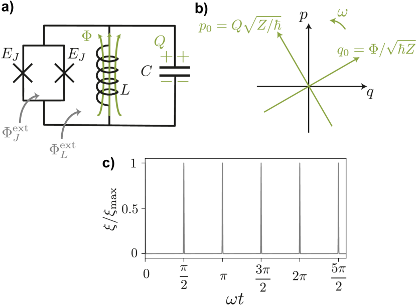
Figure 5: Engineering of the GKP Hamiltonian. a) A Josephson ring is placed in parallel of a $LC$ resonator of large impedance $Z=\sqrt{\frac{L}{C}}=2R_{Q}$. Magnetic fluxes threading the circuit loops, $\Phi_{J}^{\mathrm{ext}}(\xi)$ and $\Phi_{L}^{\mathrm{ext}}(\xi)$, both functions of a control signal $\xi$, allow to tune the circuit effective Josephson energy $2E_{J}\xi$. b) The laboratory frame flux coordinate $\Phi$ periodically aligns with the coordinates $q$ and $p$ of the frame rotating at $\omega=1/\sqrt{LC}$. c) The control signal $\xi(t)$ consists in a train of short bias pulses, so that the Josephson energy takes non-zero values at these instants only. In the RWA, the effective Hamiltonian contains modular functions of ${\bf q}$ and ${\bf p}$, with spatial frequencies $2\sqrt{\pi}$ for the chosen circuit impedance, both stemming from the Josephson modular flux operator.

For the sake of pedagogy, we now describe a control method to engineer a Hamiltonian involving the two modular stabilizers in a simple superconducting circuit. The key ideas of the protocol for modular dissipation engineering described in Sec. V are already present in this toy example. The goal here is to synthesize the GKP Hamiltonian

$${\bf H}_{\mathrm{GKP}}=-E\big{(}\mathrm{cos}(\eta{\bf q})+\mathrm{cos}(\eta{\bf p})\big{)},$$ (4)

in the rotating frame of a superconducting resonator. This Hamiltonian has a degenerate ground state corresponding to the two infinite-energy GKP states $|\pm Z_{\infty}\rangle$.

We consider the circuit pictured in Fig. 5a. The inductor and capacitor form a quantum oscillator whose conjugate variables are the flux threading the inductor $\Phi$ and the charge on the capacitor $Q$. The corresponding operators can be reduced as ${\bf q}_{0}=\frac{1}{\sqrt{\hbar Z}}{\bf\Phi}$ and ${\bf p}_{0}=\sqrt{\frac{Z}{\hbar}}{\bf Q}$, where $Z=\sqrt{L/C}$ is the circuit impedance, so as to verify $[{\bf q}_{0},{\bf p}_{0}]=i$ and to display equal fluctuations in the vacuum state. The $LC$ oscillator is placed in parallel of a ring made of two Josephson junctions with equal energy $E_{J}$. We apply two magnetic fluxes $\Phi_{J}^{\mathrm{ext}}=\varphi_{0}(\pi-2\mathrm{Arcsin}(\xi(t)))$ and $\Phi_{L}^{\mathrm{ext}}=-\Phi_{J}^{\mathrm{ext}}/2$, where $\varphi_{0}=\hbar/(2e)$ is the reduced flux quantum and $\xi$ is an AC bias signal, respectively through the Josephson ring loop and the loop formed with the inductor. In presence of these flux biases, the Josephson ring behaves as a single junction with time-varying energy and null tunneling phase [51], acting on the $LC$ resonator via the Hamiltonian

$${\bf H}_{J}(t) =-2E_{J}\xi(t)\mathrm{cos}({\bf\Phi}/\varphi_{0}).$$ (5)

Designing the circuit to have an impedance $Z=2R_{Q}$, where $R_{Q}=\frac{h}{4e^{2}}\simeq 6.5~{}\mathrm{k}\Omega$ is the resistance quantum, the circuit Hamiltonian in reduced coordinates reads

$${\bf H}_{0}(t)=\frac{\hbar\omega}{2}({\bf q}_{0}^{2}+{\bf p}_{0}^{2})-2E_{J}\xi(t)\mathrm{cos}(\eta{\bf q}_{0}),$$ (6)

where $\omega=1/\sqrt{LC}$. We now place ourselves in the interaction picture to cancel out the dynamics of the linear part of the circuit. In the $(q,p)$ frame rotating at $\omega$, the sole remaining dynamics is governed by the Josephson term, a modular function of the now rotating quadrature operator ${\bf q}_{0}(t)=\mathrm{cos}(\omega t){\bf q}+\mathrm{sin}(\omega t){\bf p}$. This operator aligns with ${\bf q}$ or ${\bf p}$ every quarter period of the oscillator (see Fig. 5b). The idea is to bias the Josephson ring with a train of short flux pulses in order to activate Josephson tunneling at these precise instants only (see Fig. 5c). Letting $\xi(t)\simeq\xi_{1}{}_{\frac{\pi}{2\omega}}(t)$ where $\xi_{1}$ is the integrated amplitude of each pulse and _T denotes a Dirac comb of period $T$, in the Rotating Wave Approximation (RWA), we obtain the effective Hamiltonian

$$\begin{split}{\bf H}_{\mathrm{RWA}}&=-2E_{J}\overline{\xi(t)\mathrm{cos}(\eta{\bf q}_{0}(t)})\\ &=-E\big{(}\mathrm{cos}(\eta{\bf q})+\mathrm{cos}(\eta{\bf p})\big{)}\\ &={\bf H}_{\mathrm{GKP}}\end{split}$$ (7)

with $E=\frac{2E_{J}\omega}{\pi}\xi_{1}$. It is straightforward to combine this doubly modular Hamiltonian with a small quadratic potential $\frac{\hbar\delta}{2}({\bf q}^{2}+{\bf p}^{2})$ with $\hbar\delta\ll E$ in order to get finite-energy GKP states as quasi-degenerate ground states [45]. Indeed, such a weakly confining potential is simply obtained by increasing the duration between the pulses of the bias train to $\frac{\pi}{2(\omega-\delta)}$.

Here, we stress that we described this method as an example of modular dynamics engineering only. It does not provide a protected qubit per se as would a circuit implementing the same Hamiltonian in the laboratory frame [6, 45]. Indeed, the GKP code states are not stable upon loss of a photon. For a system directly governed by the static Hamiltonian ${\bf H}_{\mathrm{GKP}}$ and prepared in the ground manifold, photon emission into a cold bath would violate energy conservation and photon loss thus does not occur. This argument does not hold when ${\bf H}_{\mathrm{GKP}}$ is engineered in the rotating frame from a time-dependent Hamiltonian. In that case, photon emission into the environment can occur even at zero temperature, pulling the oscillator state out of the ground manifold of ${\bf H}_{\mathrm{GKP}}$. Stabilization of the GKP code manifold could still be achieved by coupling the circuit to a colored bath engineered to enforce energy relaxation in the rotating frame [56].

V Modular dissipation engineering in a Josephson circuit

V.1 Modular dissipators from modular interactions

Armed with the previous example, we now turn to engineering the modular dissipative dynamics described in Sec. III. First, we note that the Lindblad operators (3) can be substituted with the following linear combinations

$$\begin{split}{\bf L}_{q,s}&=({\bf L}_{0}+{\bf L}_{2})/\sqrt{2}\\ {\bf L}_{q,d}&=({\bf L}_{0}-{\bf L}_{2})/(\sqrt{2}i)\\ {\bf L}_{p,s}&=({\bf L}_{1}+{\bf L}_{3})/\sqrt{2}\\ {\bf L}_{p,d}&=({\bf L}_{1}-{\bf L}_{3})/(\sqrt{2}i)\end{split}$$ (8)

Second, following a standard procedure [55], each Lindblad operator ${\bf L}_{r,l}$ with $r=q$ or $p$, $l=s$ or $d$ is obtained by coupling the target mode $a$ to an ancillary mode $b$, damped at rate $\kappa_{b}$, via an interaction Hamiltonian

$${\bf H}^{\mathrm{int}}_{k,l}=\hbar g{\bf L}_{r,l}{\bf b^{\dagger}}+h.c.$$ (9)

Indeed, adiabatically eliminating the mode $b$ in the limit $g\ll\kappa_{b}$, the two-mode dynamics reduces to a single-mode dissipative dynamics with the desired Lindblad operator ${\bf L}_{r,l}$, at a rate $\Gamma=4g^{2}/\kappa_{b}$. Third, we define rotated quadrature operators of the target and ancillary modes ${\bf r}_{a}^{\pm}=e^{\pm i\frac{\epsilon}{2\eta}{\bf a}^{\dagger}{\bf a}}~{}{\bf r}^{0}_{a}~{}e^{\mp i\frac{\epsilon}{2\eta}{\bf a}^{\dagger}{\bf a}}$ and ${\bf p}_{b}^{\pm}=e^{\pm i\frac{\eta\epsilon}{4}{\bf b}^{\dagger}{\bf b}}~{}{\bf p}_{b}~{}e^{\mp i\frac{\eta\epsilon}{4}{\bf b}^{\dagger}{\bf b}}$, where ${\bf r}^{0}_{a}={\bf q}_{a}$ for $r=q$ (respectively ${\bf r}^{0}_{a}={\bf p}_{a}$ for $r=p$), and we remark that the Hamiltonian (9) is approximated by

$$\begin{split}{\bf H}^{\mathrm{int}}_{r,l}\simeq\quad 2\hbar g~{}\big{(}&~{}~{}~{}~{}\mathcal{A}~{}\mathrm{cos}(\eta{\bf r}^{0}_{a}-\delta_{l}\frac{\pi}{2}){\bf q}_{b}\\ &+\mathcal{A}~{}\mathrm{cos}(\eta{\bf r}_{a}^{+}-\delta_{l}\frac{\pi}{2}){\bf p}_{b}^{+}\\ &-\mathcal{A}~{}\mathrm{cos}(\eta{\bf r}_{a}^{-}-\delta_{l}\frac{\pi}{2}){\bf p}_{b}^{-}\\ &-~{}(1-\delta_{l}){\bf q}_{b}~{}~{}\big{)}\end{split}$$ (10)

at first order in $\epsilon$ , with the convention $\delta_{s}=0$, $\delta_{d}=1$. The first three terms in this Hamiltonian have the same form and can be activated in the rotating frame of a two-mode Josephson circuit as described in the next section. The fourth term is trivially implemented by driving the ancillary mode resonantly.

Note that activating simultaneously four Lindblad operators necessitates four distinct ancillary modes. A hardware-efficient alternative consists in activating them sequentially, leveraging a single ancillary mode and switching from one operator to the next at a rate slower than $\kappa_{b}$—giving the ancillary mode sufficient time to reach its steady state and justifying its adiabatic elimination—but faster than $\Gamma$—accurately reproducing the target four-dissipator dynamics by Trotter decomposition. This strategy drastically reduces the experimental software complexity, at the cost of a fourfold reduction of the modular dissipation rate $\Gamma$. With these considerations in mind, we now focus on the activation of a single Lindblad operator and assume that the full target dynamics is easily derived thereof.

V.2 Activating modular interactions in the rotating frame

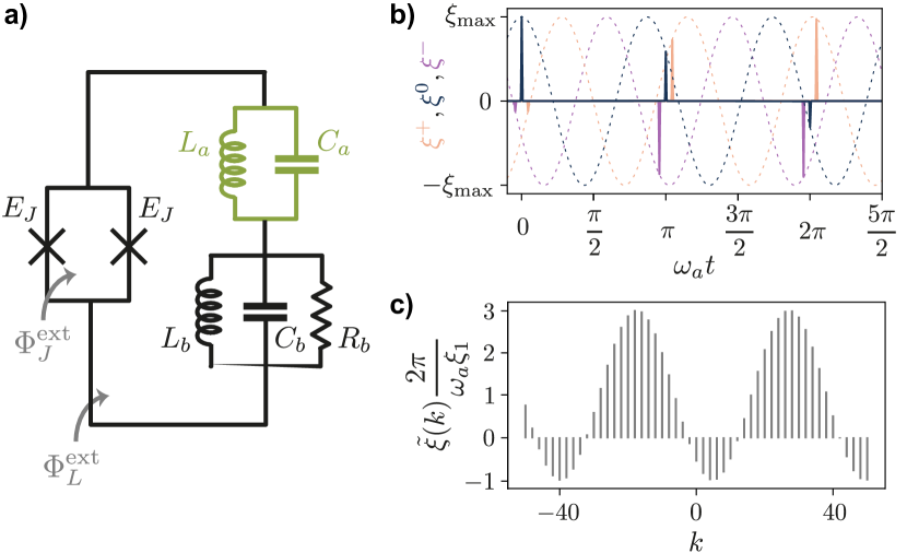
Figure 6: Engineering modular interactions. a) A Josephson ring is placed in parallel of a high-impedance target resonator (green) and a low-impedance, dissipative, ancillary resonator (black). The Josephson tunneling amplitude $2E_{J}\xi(t)$ and phase are adjusted with the control fluxes $\Phi_{J,L}^{\mathrm{ext}}$ biasing the circuit. b) Each modular Lindblad operator (8) is activated with an AC bias signal consisting in the sum of three pulse trains $\xi=\xi^{-}+\xi^{0}+\xi^{+}$ (trains respectively colored in purple, black, and orange), pulses within each train being separated by half a period of the target resonator. Each train modulates a carrier at $\omega_{b}$, the three carriers being phase-shifted by $\sim\pm\frac{\pi}{2}$ from one another (dashed lines with same colors as the pulse trains). c) In frequency domain, the bias signal $\mathcal{F}[\xi](\omega)=\sum_{k\in\mathbb{Z}}\tilde{\xi}(k)(\delta(\omega-\omega_{b}-k\omega_{a})+\delta(\omega+\omega_{b}+k\omega_{a}))$ is a real-valued frequency comb centered at $\pm\omega_{b}$ and whose amplitude $\tilde{\xi}(k)$ oscillates with a period $\frac{4\pi\eta}{\epsilon}$. The signal represented in b-c corresponds to the activation of ${\bf L}_{q,s}$ and contains only even harmonics $k\in 2\mathbb{Z}$. For readability, we set $\epsilon=1$ and $\omega_{b}=2.3~{}\omega_{a}$ in b (respectively $\omega_{b}/\omega_{a}\rightarrow\infty$ in c so that the comb does not overlap with its mirror image centered at $-\omega_{b}$), which is not the regime in Table 1.

The method and circuit to activate arbitrary modular interactions is analogous to the GKP Hamiltonian engineering technique described in Sec. IV. Here, we consider the multimode circuit pictured in Fig. 6a. The Josephson ring is shunted by the target resonator with impedance $Z_{a}=2R_{Q}$ placed in series with a low-impedance dissipative ancillary mode $b$ ($Z_{b}\ll R_{Q}$, $\kappa_{b}\sim\omega_{b}Z_{b}/R_{b}$). Note that this circuit should not necessarily represent a physical device: suffices it to represent the Foster decomposition [58, 59, 60] of a linear environment connected to the two ports of the Josephson ring.

Compared to Sec. IV, the DC flux bias point is modified following

$$\begin{split}\Phi_{J}^{\mathrm{ext}}&=\varphi_{0}\big{(}\pi+2\mathrm{Arcsin}(\xi(t))\big{)}\\ \Phi_{L}^{\mathrm{ext}}&=-\frac{\Phi_{J}^{\mathrm{ext}}}{2}+\varphi_{0}\frac{\pi}{4}\end{split}$$ (11)

in order to give a non-trivial phase to the Josephson tunneling [51]. The circuit Hamiltonian then reads

$${\bf H}_{0}(t)=\hbar\omega_{a}{\bf a^{\dagger}}{\bf a}+\hbar\omega_{b}{\bf b^{\dagger}}{\bf b}+2E_{J}\xi(t)~{}\mathrm{cos}\big{(}\frac{{\bf\Phi}}{\varphi_{0}}-\frac{\pi}{4})$$ (12)

where the generalized phase operator across the series of resonators reads ${\bf\Phi}=\varphi_{0}(\eta_{a}{\bf q}_{a}^{0}+\eta_{b}{\bf q}_{b}^{0})$, and the vacuum phase fluctuations of each mode across the Josephson ring are given by $\eta_{a}=\sqrt{2\pi Z_{a}/R_{Q}}=2\sqrt{\pi}$ and $\eta_{b}=\sqrt{2\pi Z_{b}/R_{Q}}\ll 1$. Importantly, these values do not need to be fine-tuned in circuit fabrication as one can adapt the system controls to accommodate a value of $\eta_{a}$ exceeding $2\sqrt{\pi}$ (see Sec. VI and Supplemental materials).

Placing ourselves in the rotating frame of both $a$ and $b$, the Hamiltonian becomes

$${\bf H}(t)=2E_{J}\xi(t)~{}\mathrm{cos}\big{(}\eta_{a}{\bf q}^{0}_{a}(t)+\eta_{b}{\bf q}^{0}_{b}(t)-\pi/4\big{)}$$ (13)

where the quadrature operators ${\bf q}^{0}_{a}$ and ${\bf q}^{0}_{b}$ rotate in phase-space. We now consider the AC bias signal

$$\begin{split}\xi(t)&=\sum_{j=0,+,-}\xi^{j}(t)\\ &\simeq\sum_{j=0,+,-}s_{j}\xi_{1}\big{(}{}_{\frac{2\pi}{\omega_{a}}}(t-t_{j,r})~{}+~{}\delta_{l}{}_{\frac{2\pi}{\omega_{a}}}(t-t_{j,r}-\tfrac{\pi}{\omega_{a}})\big{)}\\ &~{}~{}~{}~{}~{}~{}~{}~{}~{}~{}~{}~{}~{}~{}~{}~{}~{}~{}~{}~{}~{}~{}~{}~{}~{}~{}~{}~{}~{}~{}\times\mathrm{cos}(\omega_{b}t~{}-~{}\theta_{j})\end{split}$$ (14)

consisting in three trains of short pulses with integrated amplitude $\xi_{1}$ and sign $s_{j}$ ($s_{j}=+1$ for $j=0$ or $j=+$, $s_{j}=-1$ for $j=-$) modulating carriers at $\omega_{b}$, the pulses within each train being separated by half a period of the target resonator and having either constant ($\delta_{l}=1$) or alternating signs ($\delta_{l}=-1$). Each train is offset by $t_{j,r}$, defined as $t_{j,q}=\frac{j\epsilon}{2\eta\omega_{a}}$ and $t_{j,p}=t_{j,q}+\frac{\pi}{2\omega_{a}}$, and is responsible for the activation of one of the modular interactions in the target Hamiltonian (10) by triggering Josephson tunneling when the rotating operator ${\bf q}^{0}_{a}(t)$ aligns or anti-aligns with the corresponding target mode quadrature ${\bf r}_{a}^{j}$. If the pulses are sufficiently narrow (see Sec. VI for details) and assuming that $\omega_{a}$ and $\omega_{b}$ are not commensurable, the RWA yields only terms of the form $\mathrm{cos}(\pm\eta_{a}{\bf r}^{j}_{a})(e^{-i\theta_{j}}{\bf b}+e^{i\theta_{j}}{\bf b}^{\dagger})$ and $\mathrm{sin}(\pm\eta_{a}{\bf r}^{j}_{a})(e^{-i\theta_{j}}{\bf b}+e^{+i\theta_{j}}{\bf b}^{\dagger})$ . Finally, choosing pulses with constant ($\delta_{l}=1$) or alternating ($\delta_{l}=-1$) signs ensures that only cosine or sine operators survive the RWA—depending on which Lindblad operator is targeted—and the carrier phases $\theta_{j}=j(j\frac{\pi}{2}+\frac{\epsilon\eta}{4})$ are chosen to match the phases of each ancillary mode operator in the target Hamiltonian. In Fig. 6b-c, we represent the total bias signal when activating ${\bf L}_{q,s}$. In time domain, it consists in a train of pulse triplets, while in frequency domain, it is a frequency comb centered at $\pm\omega_{b}$ (mirror image around $-\omega_{b}$ not shown) and whose amplitude oscillates with a period $\frac{4\pi\eta}{\epsilon}\omega_{a}$. The signals activating other Lindblad operators are obtained by alternating the pulses sign in time domain and/or alternating the harmonics sign in frequency domain.

Overall, the target Hamiltonian (10) is activated at a rate $g=E_{J}\eta_{b}\omega_{a}\xi_{1}/(2\sqrt{2}\pi\hbar\mathcal{A})$. Note that to reach this effective Hamiltonian, we performed an adiabatic elimination of the ancillary mode—requiring $g\ll\kappa_{b}$—and a RWA—requiring $\kappa_{b}\ll\omega_{a}$ [55]. Moreover, we choose $\omega_{a}\ll\omega_{b}$ to avoid frequency collisions that would enable high-order processes involving multiple photons of the ancilla in the RWA. Given that protection of the logical qubit requires the modular dissipation rate $\Gamma\sim\frac{g^{2}}{\kappa_{b}}$ to be larger than the target resonator photon loss rate $\kappa_{a}$, the system parameters should respect

$$\kappa_{a}\ll g^{2}/\kappa_{b}\ll\kappa_{b}\ll\omega_{a}\ll\omega_{b}.$$ (15)

This regime is attainable in a state-of-the-art circuit (see Tab. 1) comprising a high-impedance mode resonating in the 100 MHz range. This unusually low resonance frequency is needed to respect the above hierarchy, and to ensure that flux bias pulses are sufficiently short with respect to the target oscillator period, as detailed in the next section.

VI Implementation with state-of-the-art circuits and control electronics

The goal of this section is to propose realistic experimental parameters for the stabilization of GKP qubits and to estimate the impact of various experimental imperfections. We first remind the reader that the impact of intrinsic, low-weight noise processes affecting the target resonator was analyzed in Sec. III and shown to be robustly suppressed by the modular dissipation. Here, we consider the noise sources induced by the dissipation engineering itself.

VI.1 Limited bandwidth and accuracy of the flux bias signal

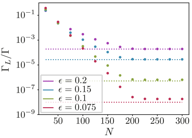
Figure 7: Truncated frequency comb. Decay rate of the generalized Pauli operators ${\bf X}$ and ${\bf Z}$ under modular dissipation engineered with a frequency comb containing a finite number of harmonics $N$ (dots), in absence of intrinsic noise of the target resonator. A finite bandwidth signal yields spurious errors at a rate decreasing exponentially with $N$. The decay rate found for $N\rightarrow\infty$ does not quantitatively match the rate found for the ideal dissipators (3) (dashed lines), which is yet to be understood.

A central hypothesis to the dissipation engineering technique detailed in Sec. III is that the width of the flux pulses that bias the circuit is negligible with respect to the target oscillator period. In frequency domain, this figure of merit directly relates to the number of harmonics $N$ in the frequency comb forming the bias signal $\xi$ (see Fig. 6c). This number should be quantitatively optimized: on the one hand, it should not be too small for the aforementioned hypothesis to hold, but picking an unnecessarily large $N$ would place prohibitive constraints on the circuit design—for a fixed control signal bandwidth, one can only increase $N$ by decreasing the target mode resonance frequency—and limit the modular dissipation rate for a given maximum value of the bias signal $\xi_{\mathrm{max}}$ .

To this end, we perform numerical simulations, in the RWA [55], considering Lindblad operators activated by a bias signal $\tilde{\xi}_{N}(k)$ obtained by truncating the Fourier series $\tilde{\xi}(k)$ (setting $\tilde{\xi}(k)=0~{}\text{for}~{}|k|>N$, see Fig. 6c for a representation of $\tilde{\xi}(k)$). The evolution of the target oscillator state is computed for the corresponding imperfect modular dissipation in absence of any other decoherence channel. The decay rate of the generalized Pauli operators ${\bf X}$ and ${\bf Z}$ is extracted for each value of $N$, and represented in Fig. 7. Truncation of the bias comb leads to spurious logical flips at a rate independent of $\epsilon$ and exponentially decreasing with $N$. In the long term, this scaling is encouraging as one does not need to increase the control signal bandwidth indefinitely to robustly protect the encoded information. In the short term, combs containing $N\sim 100$ harmonics are needed to suppress the logical error rate significantly beyond the break-even point (see Tab. 1). Limiting microwave drives to the 0-20 GHz range, which corresponds to the bandwidth of standard laboratory equipment and is below the typical plasma frequency of Josephson junctions , this places the target mode resonance frequency in the sub-GHz range (see Tab. 1).

Delivering a precise, wideband, microwave signal to a superconducting circuit cooled down in the quantum regime is a major experimental challenge. If this signal is generated at room temperature, one needs to account for a priori unknown dispersion of the feedlines. Therefore, the complex amplitudes of $2N+1$ phase-locked, monochromatic microwave signals need to be individually calibrated (see [55] for quantitative estimates of the impact of miscalibration). Recent advances in digital synthesis of microwave signals allows for the automation of these calibrations. An alternative strategy consists in generating the frequency comb directly on-chip with a dedicated Josephson circuit [64, 65] in order to deliver a precise, wideband comb with no need for complex calibrations.

VI.2 Fabrication constraints and disorder

Inaccuracy on the energy of Josephson junctions is the main source of disorder in superconducting circuits, with a typical mismatch of the order of a few percents from the targeted value to the one obtained in fabrication. In the circuit depicted in Fig. 6a, this leads to uncertainty on the value of the superinductance $L_{a}$, typically implemented by a chain of Josephson junctions [66], and to a small energy mismatch between the two ring junctions. Fortunately, these parameters do not need to be fine-tuned in our approach.

Indeed, an inductance $L_{a}$ differing from its nominal value only results in a modified target mode impedance $Z_{a}$, and therefrom in modified phase fluctuations across the Josephson ring $\eta_{a}=\sqrt{2\pi Z_{a}/R_{Q}}$. Here we remind the reader that the target value $\eta_{a}=2\sqrt{\pi}$ was chosen to match the length of the square GKP lattice unit cell. However, as detailed in Sec. VII, there exists a continuous family of GKP codes whose diamond-shaped unit cells still have an area of $4\pi$, but longer edges. As long as $\eta_{a}>2\sqrt{\pi}$, one simply adjusts the timing of flux bias pulses to stabilize such a non-square code. We verify in simulation that the accuracy with which this adjustment needs to be performed is well within reach of current experimental setups [55].

We now consider the effect of a small asymmetry of the circuit Josephson ring. We remind the reader that in our dissipation engineering scheme, the effective Josephson energy is cancelled by threading the ring with half a quantum of magnetic flux—corresponding to the DC contribution in $\Phi_{J}^{\mathrm{ext}}$—except at precise instants when it is activated with sharp flux pulses—corresponding to the AC contribution in $\Phi_{J}^{\mathrm{ext}}$. Mismatch between the two junction energies lead to imperfect cancellation in-between pulses, potentially generating shifts of the target oscillator state by $\eta_{a}$ along a random axis in phase-space (see Fig. 2). As detailed in Supplemental materials, this advert affect can be mitigated by slightly adjusting the circuit DC bias point so that the imperfectly cancelled Josephson Hamiltonian becomes non-resonant and drops out in the RWA. This RWA is only valid if the energy mismatch between junctions is much smaller than the target mode frequency $\omega_{a}$, placing a new constraint on the circuit parameters. In Tab. 1, we choose a Josephson energy as low as $E_{J}=h\times 500~{}$MHz—which we still consider experimentally realistic while keeping the junctions plasma frequency above 20 GHz [55]—such that a $2\%$ mismatch should be tolerable. We leave quantitative analysis of the robustness of this strategy for future work and note that it may be combined with the method sketched in the next section for a more robust suppression of the impact of imperfectly cancelled Josephson energy.

VI.3 $1/f$ magnetic flux noise

While its microscopic origin is still debated, low-frequency magnetic flux noise (referred to as 1/f noise) is ubiquitous in superconducting circuits [67]. In practice, such noise will induce slow drifts in the DC bias point of our proposed circuit, which cannot be detected and compensated on short ($\sim 1~{}$ms) timescales. A small offset to the magnetic flux $\Phi_{L}^{\mathrm{ext}}$ threading the rightmost loop of the circuit (see Fig. 6 and Eq. 11) is not expected to affect significantly the performances of our protocol. Indeed, it only impacts the phase of the Josephson term in (13), slightly unbalancing the rates of the engineered modular dissipators (8). On the other hand, an offset to the magnetic flux threading the Josephson ring $\Phi_{J}^{\mathrm{ext}}$ results in an imperfectly cancelled Josephson energy in between fast bias pulses, similar to that induced by a mismatch of the two junctions energy. Unfortunately, here, adapting the circuit bias to make the spurious Josephson Hamiltonian non-resonant is not an option as the magnetic flux offset is unknown. Quantifying the impact of imperfect cancellation of the Josephson energy on the lifetime of GKP qubits will be the subject of future work.

A possible strategy—not investigated in this work—to mitigate the impact of such imperfect cancellation is to dynamically vary the target mode phase fluctuations across the ring $\eta_{a}$ with a periodic window signal such that $\eta_{a}=2\sqrt{\pi}$ only on narrow windows covering the triplets of pulses forming the bias signal $\xi(t)$ (pulses represented in Fig. 6b). If $\eta_{a}\ll 2\sqrt{\pi}$ outside these windows, the imperfectly cancelled Josephson Hamiltonian only generates short displacements of the oscillator, which are corrected by the modular dissipation. Note that, although requiring a more complex circuit, controlling the value of $\eta_{a}$ is anyhow needed in order to perform protected gates on GKP qubits (see Fig. 9 for an example circuit allowing such control).

VI.4 Quasi-particle poisoning

Quasi-particles are excitations of the circuit electron fluid above the superconducting gap [68]. The probability for such excitations should be negligible at the working temperature of circuit QED experiments (10 mK), but normalized densities of quasi-particles in the range $x_{qp}\sim 10^{-5}-10^{-7}$ are typically observed. A quasi-particle with charge $e$ tunneling through the Josephson ring is expected to translate the target mode by $\pm\sqrt{\pi}$ in normalized units, which can directly lead to a logical flip. In term, this uncorrected error channel could limit the coherence time of the logical qubit. Quantitative estimates of the logical error rate induced by a given density of quasi-particles will be sought in a future work. Note that quasi-particle poisoning is detrimental to all circuitQED architectures, and is thus actively investigated. Recent progress in identifying and suppressing sources of out-of-equilibrium quasi-particles [69, 70, 71, 72], as well as in trapping and annihilating them [73, 74, 75, 76, 77, 78, 79] could conceivably lead to efficient suppression strategies in the near future.

Parameter	Symbol	Value
Target mode inductance	$L_{a}$	14 $\mu$H
(inductive energy)		($h\times$12 MHz)
Josephson junction energy	$E_{J}$	$h\times$500 MHz
Target mode capacitance	$C_{a}$	80 fF
(charging energy)		($h\times$240 MHz)
Target mode frequency	$\omega_{a}$	2$\pi\times$150 MHz
Target mode photon loss rate	$\kappa_{a}$	2$\pi\times$300 Hz
Ancillary mode frequency	$\omega_{b}$	2$\pi\times$5 GHz
Ancillary mode phase	$\eta_{b}$	0.3
fluctuations across the ring
Ancillary mode photon loss rate	$\kappa_{b}$	2$\pi\times$0.5 MHz
Number of harmonics in bias comb	$N$	100
Maximum modulation signal	$\xi_{\mathrm{max}}$	0.2
Modular interaction rate	$g$	2$\pi\times$100 kHz
Modular dissipation rate	$\Gamma$	2$\pi\times$20 kHz
Decay rate of ${\bf X}$ and ${\bf Z}$	$\Gamma_{L}$	2$\pi\times$4 Hz
Pauli operators

Table 1: Proposed circuit parameters. The target mode has an impedance $Z_{a}=2R_{Q}$ and resonates in the radio-frequency range to allow biasing of the circuit with a frequency comb containing $N=100$ harmonics within a 20 GHz bandwidth. This requires to load the circuit with an ultra-high inductance, which can be implemented at the cost of only a small number of parasitic modes appearing in the operating band [55] with state-of-the-art techniques [42]. The two Josephson junctions energy is chosen low enough that a $2\%$ energy mismatch may be compensated in situ (see Sec. VI.2), and other parameters are chosen to respect the hierarchy (15). The estimated decay rate of the generalized Pauli operators only accounts for errors induced by photon loss of the target mode and by truncation of the bias frequency comb. The latter error channel significantly dominates over the former, so that increasing further the number of harmonics in the bias comb would yield a much more robust GKP qubit.

VII Fault-tolerant Clifford gates

Following the definition given by GKP [6], we define as fault-tolerant an operation on logical qubits that does not amplify shift errors of the embedding oscillators. Therefore, a fault-tolerant operation does not significantly increase the logical error rate of the qubits being controlled compared to idling qubits. Moreover, fault-tolerance requires that no decoherence channel generating long shifts of the oscillator state be opened during the operation, and that the gate be performed exactly. In the infinite-energy code limit, GKP proposed to perform fault-tolerant Clifford gates with simple low-weight drive Hamiltonians applied to the embedding oscillators [6]. In this section, we extend this result and derive target evolutions implementing Clifford gates in the finite-energy code. In contrast with the infinite-energy code case, these evolutions are not unitary and thus not trivially driven: a practical driving scheme remains to be found. Fortunately, one can circumvent the problem by slowly varying the parameters of the dissipation described in the previous sections such that its fixed points follow the desired code states trajectory in phase-space throughout the gate. In the limit where the gate duration $T_{\mathrm{gate}}$ is much longer than $1/\Gamma_{c}$ ($\Gamma_{c}$ is the confinement rate onto the code manifold, see Sec. III), we expect dissipation to coral the target state with no additional drive, as was proposed for the control of cat qubits [80]. Quantifying the spurious logical error probability for finite-time gates time will be the subject of a future work.

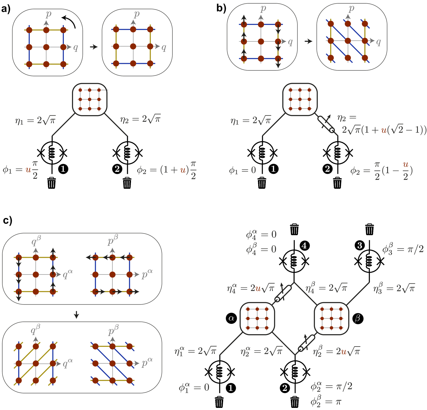
Figure 8: Clifford gates by slow variation of the modular dissipation parameters. The Hadamard (a), Phase (b) and CNOT (c) gates are each applied by continuously distorting the stabilized GKP lattice structure in phase-space. In boxes, the oscillator field states are represented by their standard deviation contours (red circles), along with the GKP lattice axes (blue and yellow) in the single mode (a-b) or bipartite (c) phase space, before and after a gate. At the end of each gate, the distorted lattice aligns with the initial one. In our proposed architecture, each oscillator is connected to at least two Josephson rings, each ring being connected to a dissipative ancillary mode (trash can icon) and responsible for the activation of a pair of Lindblad operators $({\bf L}_{r,s},{\bf L}_{r,d})$ (see Eq. 8), where $r=q$ or $p$ before and after the gate. Lattice distortion is induced by rotating the target quadrature $r$ by an angle $\phi$ (controlled by the timing of the pulses biasing the ring) and simultaneously adjusting the phase fluctuations of the oscillator across the ring $\eta$ (tunable coupling symbolized by cylinder pierced by a diagonal arrow). The parameter $u:0\rightarrow 1$ is slowly varied during the gate so that the oscillator states remain at a fixed point of the dissipation at all time.

VII.1 Clifford gates in the finite-energy GKP code

Remarkably, the target evolutions proposed by GKP to implement Clifford gates in the infinite-energy code correspond to continuous symplectic mappings of the target oscillator phase-space coordinates. In detail, for a control parameter $u$ varying continuously from 0 to 1 during the gate, these transformations read:

Hadamard gate

$$\begin{split}\mathcal{S}_{u}^{H}:\quad&{\bf q}\rightarrow\mathrm{cos}(u\frac{\pi}{2}){\bf q}+\mathrm{sin}(u\frac{\pi}{2}){\bf p}\\ &{\bf p}\rightarrow-\mathrm{sin}(u\frac{\pi}{2}){\bf q}+\mathrm{cos}(u\frac{\pi}{2}){\bf p}\end{split}$$ (16)

The corresponding evolution is a quarter turn rotation of the target state ${\bf U}^{H}_{u}=e^{iu\frac{\pi}{2}{\bf a^{\dagger}}{\bf a}}$ (see Fig. 8a).

Phase gate

$$\begin{split}\mathcal{S}^{P}_{u}:\quad&{\bf q}\rightarrow{\bf q}\\ &{\bf p}\rightarrow{\bf p}-u{\bf q}\end{split}$$ (17)

The corresponding evolution consists in squeezing and rotating the target state ${\bf U}^{P}_{u}=e^{iu{\bf q}^{2}/2}$ (see Fig. 8b).

CNOT gate

$$\begin{split}\mathcal{S}^{C}_{u}:\quad&{\bf q}^{\alpha}\rightarrow{\bf q}^{\alpha}\\ &\tilde{{\bf p}}^{\alpha}\rightarrow{\bf p}^{\alpha}-u{\bf p}^{\beta}\\ &{\bf q}^{\beta}\rightarrow{\bf q}^{\beta}+u{\bf q}^{\alpha}\\ &\tilde{{\bf p}}^{\beta}\rightarrow{\bf p}^{\beta}\end{split}$$ (18)

Here the joint evolution of the control and target oscillators labeled $\alpha$ and $\beta$ reads ${\bf U}^{P}_{u}=e^{iu{\bf q}^{\alpha}{\bf p}^{\beta}}$ (see Fig. 8c) and is the combination of two-mode squeezing and photon exchange (beam-splitter Hamiltonian).

We now note that the infinite-energy square code is entirely defined by its two stabilizers ${\bf S}_{q}=e^{i\eta{\bf q}}$ and ${\bf S}_{p}=e^{-i\eta{\bf p}}$. The code properties—namely the stabilizers and generalized Pauli operators commutation rules, the code states definition—are all inferred from the canonical commutation relation of the quadrature operators $[{\bf q},{\bf p}]=i$. Since symplectic transformations preserve commutation relations, the same modular functions of symplectically transformed variables $e^{i\eta\mathcal{S}_{u}({\bf q})}$ and $e^{-i\eta\mathcal{S}_{u}({\bf p})}$, where $\mathcal{S}_{u}$ is one of the three aforementioned transformations, are the stabilizers of another GKP code. In other words, Clifford gates are applied by continuously distorting the GKP lattice in phase-space so that the final lattice structure overlaps with the initial one, and that an exact gate has been applied to the encoded qubit (see Fig. 8). The same scheme is directly applicable to the finite-energy code, after normalizing all operators with ${\bf E}_{\Delta}=e^{-\Delta{\bf a^{\dagger}}{\bf a}}$. The target evolutions now read ${\bf V}^{\Delta}_{u}={\bf E}_{\Delta}{\bf U}_{u}{\bf E}^{-1}_{\Delta}$, and are in general non-unitary. As for the stabilizers of the distorted code, they read ${\bf E}_{\Delta}e^{i\eta\mathcal{S}_{u}({\bf q})}{\bf E}^{-1}_{\Delta}$ and ${\bf E}_{\Delta}e^{-i\eta\mathcal{S}_{u}({\bf p})}{\bf E}^{-1}_{\Delta}$. Note that with this definition, the lattice structure is distorted, but the code states normalizing envelope remains Gaussian-symmetric.

VII.2 Clifford gates by slow variation of the engineered dissipation parameters

We now detail how to adapt the dissipation engineering technique described in Sec. V to stabilize a finite-energy code distorted by $\mathcal{S}_{u}$. We consider the architecture depicted in Fig. 8, in which a target mode is connected to two rings, each one coupled to at least one dissipative ancillary mode (trash can icon). Each ring activates one pair of Lindblad operators $({\bf L}_{r,s},{\bf L}_{r,d})$ as defined in Eq. 8. For an idling logical qubit, these operators are modular functions of one of the oscillator quadratures $r=q$ or $p$. When a gate is applied, the quadrature needs to be substituted with the symplectically transformed quadrature $\mathcal{S}_{u}(r)$. First focusing on single-qubit gates, this transformed quadrature is parametrized by its angle $\phi$ and its length in phase-space. Adjusting the value of $\phi$ only requires to time-shift the control pulses biasing the corresponding ring. Indeed, these pulses are organized following a train of triplets patterns (see Fig. 6b), triplets being separated by half a period of the oscillator, and the timing of the central pulse $t$ within each half-period setting the angle $\phi$ following $\phi=2\omega_{a}t~{}\mathrm{mod}~{}2\pi$ (see Sec. V for details). The Hadamard gate (see Fig. 8a) is based on such controls only, slowly varied to respect the adiabaticity condition $\Gamma_{c}T_{\mathrm{gate}}\gg 1$. On the other hand, the phase gate necessitates to vary both the angle and length of the generalized quadrature $\mathcal{S}_{u}^{P}(p)$. Varying the latter is equivalent to adjusting the phase fluctuations $\eta$ of the target mode across the corresponding ring. In Fig. 8b, we symbolize this control by a tunable coupler (cylinder pierced by an arrow) connecting the target mode with the ring (see Fig. 9 for a more detailed circuit). Altogether, when applying a phase gate, the coupling of ring 2 to the target mode is slowly increased while the ring bias pulses are slowly time shifted in order to ramp $\phi$ and $\eta$ simultaneously.

Similar controls are employed to apply a two-mode CNOT gate. Here, two of the four transformed quadratures $\mathcal{S}^{C}_{u}(r)$—with $r=q^{\alpha},~{}p^{\alpha},~{}q^{\beta}~{}\mathrm{or}~{}p^{\beta}$—combine a fixed contribution from one mode and a varying contribution from the other one. This requires to couple with adjustable strength one of the two rings stabilizing the control oscillator to the target oscillator, and vice versa. Thus, in Fig. 8c, the coupling of ring 2—responsible for the activation of $({\bf L}_{q^{\alpha},s},{\bf L}_{q^{\alpha},d})$ when the logical qubits are idle—to the mode $\beta$ is slowly ramped up during the gate. As a consequence, the ring witnesses increasing phase fluctuations $\eta^{\beta}_{2}$ from the oscillator $\beta$, while the phase fluctuations $\eta^{\alpha}_{2}$ from the mode $\alpha$ remain constant. Moreover, the ring bias signal, which consists in a train of pulse triplets separated by half a period of mode $\alpha$ when the qubits are idle, is enriched with a second train of pulses during the gate, separated by half a period of mode $\beta$. They both modulate the same carriers at the frequency of the ancillary mode attached to the ring 2. Similar controls are applied to the ring 4, responsible for the other pair of varied Lindblad operators.

A few comments are in order about these gates and the proposed architecture. First, we remind the reader that once the evolution implementing a gate is complete, the GKP lattice of each oscillator retrieves its initial square structure. As a consequence, the control parameters $\phi$ and $\eta$, which have been varied throughout the gate, can be returned to their initial values. While the parameters variation needs to be slow during the gate, this last adjustment can be made on a much shorter timescale. The flux pulse trains biasing the ring being controlled should be interrupted during this stage in order not to inadvertently generate a modular dissipation misaligned with the oscillator GKP lattice. Second, when not applying a CNOT gate, the phase fluctuations $\eta_{2}^{\beta}$ and $\eta_{4}^{\alpha}$ need not be perfectly nullified. Indeed, spurious phase fluctuations of a mode across a ring have negligible impact as long as they are much smaller than $2\sqrt{\pi}$, since the ring can then only generate short, correctable displacements of the mode. As Supplemental materials, we propose, based on similar arguments, a protected readout strategy for the logical qubits, which does not introduce spurious dephasing out of measurement times.

VII.3 Example circuit for single and two-qubit Clifford gates

In Fig. 9, we give a more concrete example circuit implementing the architecture of Fig. 8. The phase variables of the two modes supporting logical qubits, labelled $\alpha$ and $\beta$, are defined across two capacitors (in green). Each capacitor is placed in series with two Josephson rings, each ring being coupled to an ancillary dissipative mode (in brown) via a small shared inductance $L_{c}$, neglected in the following. Furthermore, the rings shunt inductances are made tunable—for instance by implementing them with chains of Josephson rings controlled with an external magnetic field (not shown)—and a fraction of the shunt inductance of rings 2 and 4 is shared between the two target modes owing to the horizontal cross-connection. Altogether, adjusting the value of all inductances allows one to control the phase fluctuations of each target mode across one or two rings, as in the architecture of Fig. 8c. In detail, for the mode $\alpha$, these read $\eta_{i}^{\alpha}=p_{i}(\frac{\pi}{R_{Q}})^{1/2}(\frac{L^{\alpha}}{C})^{1/4}$ where $L^{\alpha}=L^{\alpha}_{1}+L^{\alpha}_{2}+L^{\alpha}_{4}$ is the total inductance shunting the capacitance $C^{\alpha}$, and $p_{i}=\frac{L^{\alpha}_{i}}{L^{\alpha}}$ for $i=1,2,4$ is the participation ratio of the inductance $i$. Similar formulas are derived for the mode $\beta$. Note that it is straightforward to extend this circuit to support a larger number of logical qubits, with a connectivity solely limited by the number of rings in which a mode can participate with large phase fluctuations.

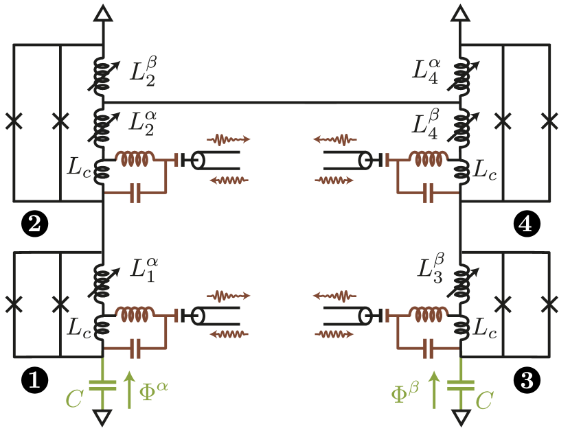
Figure 9: Example circuit stabilizing two controllable qubits. The logical qubits are encoded in two target oscillators labeled $\alpha$ and $\beta$, each supported by a capacitor (green) shunted by Josephson rings. Each ring couples to a dissipative ancillary mode (brown) through a small shared inductance. All rings have tunable shunt inductances (pierced by diagonal arrows), and the horizontal cross-connection ensures that the rings 2 and 4 participate in both modes. Varying all inductances allows adjusting independently the phase fluctuations of each mode across the rings 2 and 4, and the phase fluctuations of mode $\alpha$ (respectively $\beta$) in the ring 1 (respectively 2). By slowly varying these control parameters along with the timing of the pulse trains biasing each ring (not shown), one applies an arbitrary, fault-tolerant, Clifford gate to the encoded qubits.

VIII Conclusion and outlook

In this paper, we have proposed a novel scheme to generate, error-correct and control GKP qubits encoded in a high-impedance Josephson circuit by dissipation engineering. Numerical simulations indicate that logical errors of the encoded qubits stemming from most error channels are exponentially suppressed when the engineered dissipation rate increases. In a state-of-the-art circuit, the logical qubit lifetime could extend orders of magnitude beyond the single photon dwell time in the embedding resonator, a feat never realized so far. Arguably, at this level of error suppression, quasi-particle poisoning, which opens an uncorrected error channel, could limit the device performances. Steady progress in understanding and controlling sources of quasi-particles in superconducting devices [69, 70, 71] could conceivably overcome this roadblock in the near future.

The circuit we propose to embed multiple GKP qubits controllable with protected Clifford gates is remarkably simple (see Fig. 9) and is fabricated in a parameter regime which, though demanding (see Table 1), should prove easier to achieve than alternative proposals to encode GKP qubits at the hardware level [39, 40, 45]. Moreover, circuit parameters do not necessitate fine-tuning so that our protocol is robust against fabrication disorder. Schematically, such robustness and ease of fabrication is made possible by transferring the complexity of quantum error-correction from the hardware to the microwave control domain. Indeed, our system needs to be driven with a precise microwave frequency comb spanning a 20 GHz range. Recent progress in digital synthesis of microwaves should prove instrumental in generating and delivering such a broadband signal with sufficient accuracy. Alternatively, direct on-chip synthesis of microwave frequency combs appears compatible with the circuits we consider [64, 65], and would drastically reduce control complexity.

On the long term, the relative simplicity of Clifford gates and the robustness of our multi-GKP qubit architecture to spurious microwave cross-talks paves the way for the concatenation of these bosonic qubits into a discrete variable code such as the surface code  [81, 82, 83, 84, 85]. Given that the coherence time of GKP qubits stabilized by modular dissipation should extend far beyond single and two-qubit gate time—which is set by the confinement rate onto the code manifold in our approach—the hope is that such a surface-GKP code would operate well below threshold, implementing a fault-tolerant, universal quantum computer with minimum hardware overhead.

[maintext]

Supplemental Material

[supmat] [supmat]l1

Contents

S1 Error correction by modular dissipation in the hexagonal GKP code

One can define GKP grid states associated to lattices in phase-space that are not necessarily rectangular [6]. Of particular interest is the hexagonal GKP codespace, spanned by grid states supported along a hexagonal lattice in phase-space [7]. In particular, we will see that thanks to the symmetry of the hexagonal lattice, eigenstates of the ${\bf X},{\bf Y}$ and ${\bf Z}$ Pauli operators on the hexagonal GKP codespace have the same lifetime, whereas ${\bf Y}$ eigenstates decay twice faster than ${\bf X}$ or ${\bf Z}$ eigenstates on a square GKP codespace. The experimental stabilization of hexagonal GKP grid states has already been demonstrated using stabilizer measurement via low-weight interactions in superconducting circuits [30] and trapped ions [31] platforms. Let us explain how our dissipative stabilization scheme can be adapted to the stabilization of the hexagonal GKP codespace.

Similarly to the square case, we can define the hexagonal GKP codespace as the common $+1$ eigenspace of the six commuting stabilizer operators

$${\bf S}_{k}=e^{i\eta\,{\bf q}(\theta_{k})},\quad 0\leq k\leq 5$$ (S1)

for $\eta=2\sqrt{\frac{2\pi}{\sqrt{3}}}$, $\theta_{k}=k\pi/3$ and ${\bf q}(\theta)=e^{i\theta{\bf N}}\,{\bf q}\,e^{-i\theta{\bf N}}=\cos(\theta){\bf q}+\sin(\theta){\bf p}.$ More precisely, the same codespace could be defined using only ${\bf S}_{0}$ and ${\bf S}_{2}$, to which we add their images by successive $\pi/3$ rotations in phase space to respect the symmetry of the hexagonal grid. Note that $\eta$ is chosen such that $\eta^{2}\sin(\pi/3)=4\pi$ as before. The logical coordinates associated to any density operator are defined as the expectation values of the three generalized Pauli operators

$${\bf Z} =\mathrm{Sgn}(\cos(\tfrac{\eta}{2}{\bf q})),$$ (S2)

$${\bf X} =\mathrm{Sgn}(\cos(\tfrac{\eta}{2}{\bf q}(\tfrac{2\pi}{3}))),$$

$${\bf Y} =i{\bf Z}{\bf X}.$$

Note that ${\bf S}_{k}^{\dagger}={\bf S}_{k+3\textrm{ mod }6}$ and ${\bf X},{\bf Y},{\bf Z}$ satisfy the Pauli algebra composition rules and commute with the stabilizers.

We can introduce the corresponding finite-energy stabilizers

$${\bf S}_{k}^{\Delta}={\bf E}_{\Delta}{\bf S}_{k}{\bf E}_{\Delta}^{-1}$$ (S3)

with ${\bf E}_{\Delta}=e^{-\Delta{\bf a}^{\dagger}{\bf a}}$ and the associated Lindblad operators

$${\bf M}_{k}={\bf S}_{k}^{\Delta}-{\bf 1}.$$ (S4)

These Lindblad operators being once again a combination of trigonometric and hyperbolic functions of ${\bf q}$ and ${\bf p}$, we approximate them to first order in $\Delta$ by products of trigonometric and linear functions of ${\bf q}$ and ${\bf p}$ as

$${\bf L}_{k}=\mathcal{A}{\bf R}_{\frac{k\pi}{3}}\,e^{i\eta{\bf q}}\left({\bf 1}-\epsilon{\bf p}\right){\bf R}_{\frac{k\pi}{3}}^{\dagger}-{\bf 1}$$ (S5)

with $\epsilon=\eta\sinh\Delta$ and $\mathcal{A}=e^{-\epsilon\eta/2}$.

Finally, we propose to stabilize the hexagonal GKP codespace using the following Lindblad-type dynamics with $6$ dissipators:

$$\frac{d}{dt}\bm{\rho}=\Gamma\sum_{k=0}^{5}{\bf L}_{k}\bm{\rho}{\bf L}_{k}^{\dagger}-\frac{1}{2}\left({\bf L}_{k}^{\dagger}{\bf L}_{k}\bm{\rho}+\bm{\rho}{\bf L}_{k}^{\dagger}{\bf L}_{k}\right).$$ (S6)

Formally, the only differences with the dynamics stabilizing the square GKP codespace is that $\eta=2\sqrt{\frac{2\pi}{\sqrt{3}}}$ (instead of $\eta=2\sqrt{\pi}$), we now use $6$ dissipators (instead of $4$), related to each other by repeated rotations of $\pi/3$ (instead of $\pi/2$) in phase-space.

Crucially, the method proposed in Section V for the engineering of the modular dissipators stabilizing the square GKP codespace can be straightforwardly adapted to engineer these $6$ new dissipators. Indeed, in both cases, we describe how to engineer one of the required dissipators; the engineering of the remaining three (square case) or five (hexagonal case) is easily deduced therefrom (see Section V, or Section S3 for more details).

We can numerically compute the effective logical error rates induced by additional low-weight noise channels entering the Lindblad dynamics Eq. S6. In Fig. S1, for typical noise channels, we represent the logical error rate extracted by spectral analysis of the Lindblad superoperator (dashed lines) (see Section S2.1), in quantitative agreement with a full Lindblad master equation simulation (dots). We observe results qualitatively similar to that of Fig. 4 (corresponding to the same comparison for the square case). Note that the asymptotic logical error rates in the small noise regime appear to be lower in these simulations than the corresponding logical error rates in the square GKP simulations presented in Fig. 4. However, in realistic physical implementations, this effect would be partly compensated by the fact that the dissipators appearing in the Lindblad dynamics of Eq. S6 would be activated sequentially to leverage a single ancillary mode (see Section V). With this strategy, the effective modular dissipation rate $\Gamma$ is divided by the number of dissipators to engineer, and is thus weaker by a factor $4/6$ in the hexagonal case.

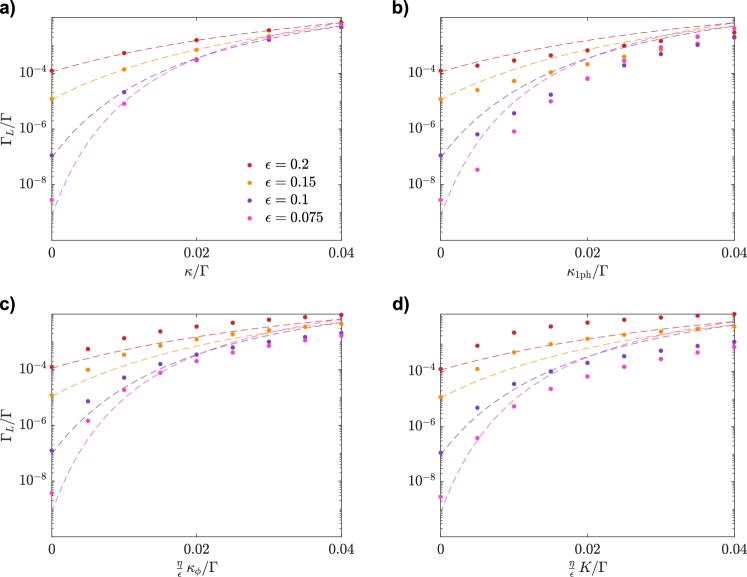
Figure S1: GKP qubit protection by modular dissipation, hexagonal code. Logical error rates are extracted from numerical simulations (dots) when varying the strength of some intrinsic noise channel relative to the modular dissipation rate $\Gamma$. For all low-weight noise channels considered, errors appear to be exponentially suppressed in the weak noise limit. a) Quadrature noise modeled by two Lindblad operators $\sqrt{\kappa}{\bf q}$ and $\sqrt{\kappa}{\bf p}$. Dashed lines are predictions by spectral analysis of the Lindblad superoperator (see Section S2.1). b) Single-photon dissipation modeled by a Lindblad operator $\sqrt{\kappa_{1\mathrm{ph}}}{\bf a}$. c) Pure dephasing modeled by a Lindblad operator $\sqrt{\kappa_{\phi}}{\bf a}^{\dagger}{\bf a}$. d) Kerr Hamiltonian perturbation of the form $\frac{K}{2}({\bf a}^{\dagger}{\bf a})^{2}$. For (c-d), note the rescaling of the x-axis by $2\bar{n}=\eta/\epsilon$. For (b-d), dashed gray lines reproduce the dashed colored lines in (a), un-rescaled, for comparison.

S2 Analytical and numerical analysis of the modular dissipation

S2.1 Exponential convergence to the code manifold and explicit decoherence rates

If one were able to directly engineer the Lindblad operators ${\bf M}_{k}$ of Section III, involving both trigonometric and hyperbolic functions of the quadrature operators ${\bf q}$ and ${\bf p}$, it was shown in [53] that the resulting Lindblad dynamics would stabilize exactly the finite-energy GKP codespace, with exponential convergence of any initial state towards the codespace. This is no longer true with the approximate Lindblad operators ${\bf L}_{k}$ in our proposal; most notably, the approximate Lindblad operators fail to perfectly vanish on the GKP codespace, which is consequently only metastable under our stabilization scheme. In other words, even without any additional dissipation channel, the encoded qubit suffers from intrinsic residual logical decoherence. We are able to explicitly compute the associated decoherence rates, and the evolution of the encoded logical qubit, without solving the Lindblad equation. Additionally, we are able to extend this result to the case where additional dissipation is added to the dynamics in the form of quadrature noise only.

Indeed, for both the square and the hexagonal GKP code, the coordinates of the encoded logical qubit are defined as expectation values of the generalized Pauli operators ${\bf X},{\bf Y},{\bf Z}$. Crucially, these operators are separable periodic observables of the form

$${\bf h}=h({\bf q}_{1},{\bf q}_{2})=f(\tfrac{\eta}{2}{\bf q}_{1})\,g(\tfrac{\eta}{2}{\bf q}_{2})$$ (S7)

where $f$ and $g$ are real-valued $2\pi$-periodic functions and $\eta=2\sqrt{\pi}$, ${\bf q}_{1}={\bf q}$, ${\bf q}_{2}={\bf q}(\pi/2)={\bf p}$ for the square code, while $\eta=2\sqrt{\frac{2\pi}{\sqrt{3}}}$, ${\bf q}_{1}={\bf q}$, ${\bf q}_{2}={\bf q}(2\pi/3)=\cos(2\pi/3){\bf q}+\sin(2\pi/3){\bf p}=-\frac{1}{2}{\bf q}+\frac{\sqrt{3}}{2}{\bf p}$ for the hexagonal code. In the two cases,

$$\left[\eta\,{\bf q}_{1},\frac{\eta}{2}\,{\bf q}_{2}\right]=\left[\frac{\eta}{2}\,{\bf q}_{1},\eta\,{\bf q}_{2}\right]=2i\pi$$ (S8)

so that by expanding the periodic functions $f$ and $g$ in Fourier series and applying the Baker-Campbell-Hausdorff formula we get

$$\left[f(\tfrac{\eta}{2}{\bf q}_{1}),\,e^{i\eta{\bf q}_{2}}\right]=\left[g(\tfrac{\eta}{2}{\bf q}_{2}),\,e^{i\eta{\bf q}_{1}}\right]=0.$$ (S9)

In the following subsections, we show that, for a density operator $\bm{\rho}$ governed by the Lindblad equation proposed earlier to stabilize the square (or hexagonal) GKP code, we can leverage Eq. S9 to compute explicitly the evolution of the average value $\operatorname{Tr}({\bf h}\bm{\rho}_{t})$, and thus in particular the evolution of the three generalized Pauli operators ${\bf X},{\bf Y},{\bf Z}$, without computing the solution $\bm{\rho}_{t}$ of the Lindblad equation. More precisely, we show that

$$\frac{d}{dt}\operatorname{Tr}({\bf h}\bm{\rho}_{t})=-\mathcal{A}\epsilon\eta\Gamma\,\operatorname{Tr}(\mathcal{L}_{\sigma}(h)({\bf q}_{1},{\bf q}_{2})\bm{\rho}_{t})$$ (S10)

where $\mathcal{A}=e^{-\frac{\epsilon\eta}{2}}$, $\Gamma>0$ is the engineered dissipation rate, $\sigma>0$ is a parameter depending on $\eta,\epsilon$ and $\mathcal{L}_{\sigma}$ is an explicit differential operator on periodic functions which depends on $\sigma$ and the geometry (square or hexagonal). $\mathcal{L}_{\sigma}$ is diagonalizable and has a positive and discrete spectrum $(\lambda_{k,\sigma})_{k\in\mathbb{N}}$. As a consequence, when $h$ is an eigenfunction of $\mathcal{L}_{\sigma}$ associated to a given eigenvalue $\lambda$, Eq. S10 leads to

$$\operatorname{Tr}({\bf h}\bm{\rho}_{t})=e^{-\mathcal{A}\epsilon\eta\Gamma\,\lambda\,t}\operatorname{Tr}({\bf h}\bm{\rho}_{0}).$$ (S11)

In the general case,

$$\operatorname{Tr}({\bf h}\bm{\rho}_{t})=\sum_{k=0}^{+\infty}c_{k}e^{-\mathcal{A}\epsilon\eta\Gamma\,\lambda_{k,\sigma}\,t}\operatorname{Tr}(h_{k,\sigma}({\bf q}_{1},{\bf q}_{2})\bm{\rho}_{0})$$ (S12)

where $h_{k,\sigma}$ is the eigenfunction of $\mathcal{L}_{\sigma}$ associated to the eigenvalue $\lambda_{k,\sigma}$ and $h=\sum_{k}c_{k}h_{k}$. Computing the spectrum of $\mathcal{L}_{\sigma}$ is thus sufficient to study the evolution of the coordinates of the encoded logical qubit, and hence to derive decoherence rates as a function of $\sigma$. The precise derivation of the differential operator $\mathcal{L}_{\sigma}$, along with an asymptotic analysis of its spectral properties in the regime $\sigma\ll 1$, can be found in the separate publication [87]. We recall the main results here for the sake of completeness. We then explain how to go beyond that asymptotic analysis by numerically computing the spectrum of $\mathcal{L}_{\sigma}$ for a given finite value of $\sigma>0$.

Finally, in presence of quadrature noise, i.e. additional dissipators in ${\bf q}$ and ${\bf p}$ entering the Lindblad dynamics, Eq. S10 still holds true with $\sigma$ now also depending on the strength of the new dissipators. Unfortunately, for other types of noise (namely photon-loss, dephasing and Kerr nonlinearities), this shortcut, whose proof depended on commutation relations between the Lindblad operators in the dynamics and periodic observables, no longer applies. In these cases, we can only rely on a full simulation of the Lindblad dynamics. We still find that these decoherence channels result in errors rates qualitatively similar to those previously computed with our eigenvalue analysis in the case of quadrature noise (see Fig. 4 and Fig. S1).

These results are to be put into perspective with the initial intuition behind the GKP bosonic code: logical states, although they are designed for robustness against small phase-space shifts thanks to the separation of their support in phase-space, should also be robust to noise processes involving only small polynomials in ${\bf a}$ and ${\bf a}^{\dagger}$, since the effects of such processes over a small time-interval can be approximated as combinations of small phase-space shifts [6].

S2.1.1 Square GKP

The generalized Pauli operators of the square GKP code are defined from the code stabilizers ${\bf S}_{q}=e^{i\eta{\bf q}}$ and ${\bf S}_{p}=e^{-i\eta{\bf p}}$ (where $\eta=2\sqrt{\pi}$) by

$$\begin{split}{\bf Z}&=\mathrm{Sgn}(\cos(\tfrac{\eta}{2}{\bf q})),\\ {\bf X}&=\mathrm{Sgn}(\cos(\tfrac{\eta}{2}{\bf p})),\\ {\bf Y}&=i{\bf Z}{\bf X}\end{split}$$ (S13)

which are indeed products of periodic functions of ${\bf q}$ and ${\bf p}$.

In the main text, we proposed to stabilize a finite-energy square GKP codespace by engineering a dissipative Lindblad dynamics

$$\frac{d}{dt}\bm{\rho}=\Gamma\,\sum_{k=0}^{3}\mathcal{D}[{\bf L}_{k}](\bm{\rho})$$ (S14)

where $\Gamma>0$, $\epsilon>0$, $\mathcal{A}=e^{-\epsilon\eta/2}$, $\mathcal{D}[{\bf L}](\bm{\rho})={\bf L}\bm{\rho}{\bf L}^{\dagger}-\frac{1}{2}\left({\bf L}^{\dagger}{\bf L}\bm{\rho}+\bm{\rho}{\bf L}^{\dagger}{\bf L}\right)$ and

$${\bf L}_{k}=\mathcal{A}e^{ik\tfrac{\pi}{2}{\bf N}}\,e^{i\eta{\bf q}}\left({\bf 1}-\epsilon{\bf p}\right)\,e^{-ik\tfrac{\pi}{2}{\bf N}}-{\bf 1}.$$ (S15)

Let us now compute the evolution under Eq. S14 of any separable periodic observables of the form

$${\bf h}=h({\bf q},{\bf p})=f(\tfrac{\eta}{2}{\bf q})\,g(\tfrac{\eta}{2}{\bf p})$$ (S16)

where $f$ and $g$ are real-valued $2\pi$-periodic functions:

$$\frac{d}{dt}\operatorname{Tr}({\bf h}\bm{\rho}_{t}) =\operatorname{Tr}({\bf h}\frac{d}{dt}\bm{\rho}_{t})=\Gamma\sum_{k=0}^{3}\operatorname{Tr}\left({\bf h}\,\mathcal{D}[{\bf L}_{k}](\bm{\rho}_{t})\right)=\Gamma\sum_{k=0}^{3}\operatorname{Tr}\left(\mathcal{D}^{*}[{\bf L}_{k}]({\bf h})\,\bm{\rho}_{t}\right)$$ (S17)

where

$$\mathcal{D}^{*}[{\bf L}_{k}]({\bf h}):={\bf L}_{k}^{\dagger}\,{\bf h}\,{\bf L}_{k}-\frac{1}{2}\left({\bf L}_{k}^{\dagger}{\bf L}_{k}\,{\bf h}+{\bf h}\,{\bf L}_{k}^{\dagger}{\bf L}_{k}\right)=\frac{1}{2}\left({\bf L}_{k}^{\dagger}\,[{\bf h},{\bf L}_{k}]+[{\bf L}_{k}^{\dagger},{\bf h}]\,{\bf L}_{k}\right).$$ (S18)

Using the relations of Eq. S9 (along with the relation $[f({\bf A}),{\bf B}]=f^{\prime}({\bf A})\,[{\bf A},{\bf B}]$ whenever $[{\bf A},\,[{\bf A},{\bf B}]]=0$) one is able to show that

$$\Gamma\sum_{k=0}^{3}\mathcal{D}^{*}[{\bf L}_{k}]({\bf h}) =-\mathcal{A}\epsilon\eta\Gamma\,\left[\left(\sin(\eta{\bf q})f^{\prime}(\tfrac{\eta}{2}{\bf q})-\frac{\mathcal{A}\epsilon\eta}{4}f^{\prime\prime}(\tfrac{\eta}{2}{\bf q})\right)g(\tfrac{\eta}{2}{\bf p})+f(\tfrac{\eta}{2}{\bf q})\left(\sin(\eta{\bf p})g^{\prime}(\tfrac{\eta}{2}{\bf p})-\frac{\mathcal{A}\epsilon\eta}{4}g^{\prime\prime}(\tfrac{\eta}{2}{\bf p})\right)\right]$$ (S19)

$$=-\mathcal{A}\epsilon\eta\Gamma\,\mathcal{L}_{\sigma}(h)(\tfrac{\eta}{2}{\bf q},\tfrac{\eta}{2}{\bf p})$$

where $\sigma=\frac{\mathcal{A}\epsilon\eta}{4}$ and $\mathcal{L}_{\sigma}$ is the differential operator defined by

$$\mathcal{L}_{\sigma} =\mathcal{T}_{\sigma}\otimes{\bf 1}+{\bf 1}\otimes\mathcal{T}_{\sigma},$$ (S20)

$$(\mathcal{T}_{\sigma}f)(\theta) =\sin(2\theta)f^{\prime}(\theta)-\sigma f^{\prime\prime}(\theta)$$

(we refer to [87] for the detailed computation).
A straightforward computation shows, through integration by parts, that for any $2\pi$-periodic functions $f$ and $g$:

$$\langle f,\,\mathcal{T}_{\sigma}g\rangle_{\sigma} =\langle\mathcal{T}_{\sigma}f,\,g\rangle_{\sigma}$$ (S21)

$$\langle f,\,\mathcal{T}_{\sigma}f\rangle_{\sigma} =\sigma\,\langle f^{\prime},\,f^{\prime}\rangle_{\sigma}$$

for the scalar product $\langle\cdot,\cdot\rangle_{\sigma}$ defined as

$$\langle f,g\rangle_{\sigma}=\int_{-\pi}^{\pi}e^{-\frac{1-\cos(2\theta)}{2\sigma}}f(\theta)^{*}g(\theta)d\theta.$$ (S22)

Eq. S21 can also be obtained by observing that the following relation holds:

$$w_{\sigma}\mathcal{T}_{\sigma}(f)=-\sigma\left(w_{\sigma}f^{\prime}\right)^{\prime}$$ (S23)

where we introduced a weight function $w_{\sigma}(\theta)=e^{-\frac{1-\cos(2\theta)}{2\sigma}}$ (note that $\langle f,g\rangle_{\sigma}=\int w_{\sigma}f^{*}g$). As a consequence, $\mathcal{T}_{\sigma}$ is self-adjoint for the scalar product $\langle\cdot,\cdot\rangle_{\sigma}$ and non-negative; classical results show that its spectrum is thus discrete, real and non-negative (see e.g. [88]). Moreover, using Eq. S20, we can easily deduce the eigenvalues of $\mathcal{L}_{\sigma}$ from that of $\mathcal{T}_{\sigma}$: if

$$\mu_{0,\sigma}\leq\mu_{1,\sigma}\leq\mu_{2,\sigma}\,\ldots$$ (S24)

denote the eigenvalues of $\mathcal{T}_{\sigma}$ sorted in ascending order, where each $\mu_{k,\sigma}$ is associated to an eigenfunction $f_{k,\sigma}$, then the eigenvalues of $\mathcal{L}_{\sigma}$ are the sums

$$\lambda_{k_{1},k_{2},\sigma}=\mu_{k_{1},\sigma}+\mu_{k_{2},\sigma},$$ (S25)

associated to the eigenfunctions

$$h_{k_{1},k_{2},\sigma}=f_{k_{1},\sigma}\otimes f_{k_{2},\sigma}.$$ (S26)

It is thus sufficient to compute the eigenvalues and eigenfunctions of $\mathcal{T}_{\sigma}$.

Note that $\mu_{0,\sigma}=0$ is always an eigenvalue of $\mathcal{T}_{\sigma}$ associated to the eigenfunction $f\equiv 1$, so that $\lambda_{0,\sigma}=0$ is an eigenvalue of $\mathcal{L}_{\sigma}$ associated to the eigenfunction $h\equiv 1\otimes 1=1$. This simply correspond to the trivial identity

$$\frac{d}{dt}\operatorname{Tr}(\bm{\rho}_{t})=0.$$ (S27)

In the limit $\sigma\rightarrow 0$, the other eigenvalues of $\mathcal{T}_{\sigma}$ have been rigorously studied in [87] (using mathematical results from [89]), where the following asymptotics estimates were obtained:

$$\mu_{1,\sigma} \sim\frac{4}{\pi}e^{-1/\sigma},$$ (S28)

$$\mu_{2,\sigma} \geq\upepsilon_{0}>0$$

where $\upepsilon_{0}$ is a fixed constant independent of $\sigma$.

In particular, for small enough $\sigma$, $2\mu_{1,\sigma}\ll\mu_{2,\sigma}$ so that the first eigenvalues of $\mathcal{L}_{\sigma}$ read:

$$\lambda_{0,\sigma} =\lambda_{0,0,\sigma}=0,$$ (S29)

$$\lambda_{1,\sigma} =\lambda_{0,1,\sigma}=0+\mu_{1,\sigma}=\mu_{1,\sigma},$$

$$\lambda_{2,\sigma} =\lambda_{1,0,\sigma}=\mu_{1,\sigma}+0=\mu_{1,\sigma},$$

$$\lambda_{3,\sigma} =\lambda_{1,1,\sigma}=2\,\mu_{1,\sigma},$$

where the notation with single indices $\lambda_{k,\sigma}$ denotes eigenvalues of $\mathcal{L}_{\sigma}$ sorted in ascending order, whereas the notation with doubles indices $\lambda_{k_{1},k_{2},\sigma}$ indicates how they are obtained as sums of eigenvalues of $\mathcal{T}_{\sigma}$.

Finally, apart from these asymptotic results, we can turn to numerical diagonalization of $\mathcal{T}_{\sigma}$ to compute the exact value of $\lambda_{k,\sigma}$ for a fixed value of $\sigma$. To that end, note that $\mathcal{T}_{\sigma}$ has a simple expression in the Fourier frame: indeed, writing any (smooth) $2\pi$-periodic function $f$ as

$$f(\theta)=\sum_{k\in\mathbb{Z}}f_{k}e^{ik\theta},$$ (S30)

we get

$$(\mathcal{T}_{\sigma}f)(\theta) =\sin(2\theta)f^{\prime}(\theta)-\sigma f^{\prime\prime}(\theta)$$ (S31)

$$=\sum_{k\in\mathbb{Z}}\left(ik\,\frac{e^{2i\theta}-e^{-2i\theta}}{2i}+\sigma k^{2}\right)\,f_{k}\,e^{ik\theta}$$

$$=\sum_{k\in\mathbb{Z}}\left(\frac{k-2}{2}f_{k-2}-\frac{k+2}{2}f_{k+2}+\sigma k^{2}f_{k}\right)e^{ik\theta}.$$

In the Fourier frame, $\mathcal{T}_{\sigma}$ can thus be approximated by a tri-diagonal matrix by truncating the sum above to $-K_{\textrm{max}}\leq k\leq K_{\textrm{max}}$ (i.e. bounding the maximum frequency considered). On Fig. S2 we compare the numerical eigenvalues obtained by this procedure to the explicit asymptotic expressions of Eq. S28, together with the numerical eigenfunction $f_{1,\sigma}$ corresponding to the first non-zero eigenvalue $\mu_{1,\sigma}$ for different values of $\sigma$. We observe that

$$f_{1,\sigma}(\theta)\xrightarrow[\sigma\rightarrow 0]{}\operatorname{Sign}(\cos(\theta)).$$ (S32)

Hence, combining Eqs. S26, S29 and S32 (and estimating $\upepsilon_{0}$ from the numerically computed eigenvalues) we obtain that the first eigenvalues and eigenfunctions of $\mathcal{L}_{\sigma}$ in the limit of small $\sigma$ are given by

$$\lambda_{0,\sigma} =0 \quad h_{0,\sigma}(\theta_{1},\theta_{2}) =1$$ (S33)

$$\lambda_{1,\sigma} =\mu_{1,\sigma}\sim\frac{4}{\pi}e^{-1/\sigma} \quad h_{1,\sigma}(\theta_{1},\theta_{2}) =f_{1,\sigma}(\theta_{1})\simeq\operatorname{Sign}(\cos(\theta_{1}))$$

$$\lambda_{2,\sigma} =\mu_{1,\sigma}\sim\frac{4}{\pi}e^{-1/\sigma} \quad h_{2,\sigma}(\theta_{1},\theta_{2}) =f_{1,\sigma}(\theta_{2})\simeq\operatorname{Sign}(\cos(\theta_{2}))$$

$$\lambda_{3,\sigma} =2\,\mu_{1,\sigma}\sim\frac{8}{\pi}e^{-1/\sigma} \quad h_{3,\sigma}(\theta_{1},\theta_{2}) =f_{1,\sigma}(\theta_{1})f_{1,\sigma}(\theta_{2})\simeq\operatorname{Sign}(\cos(\theta_{1}))\operatorname{Sign}(\cos(\theta_{2}))$$

$$\lambda_{n,\sigma} \geq\lambda_{4,\sigma}=\mu_{2,\sigma}\geq\upepsilon_{0}\gtrsim 1 \quad\forall n\geq 4.$$

Crucially, coming back to periodic observables on the stabilized GKP qubit, Eq. S33 leads to the three observables

$${\bf h}_{1,\sigma} =h_{1,\sigma}(\tfrac{\eta}{2}{\bf q},\tfrac{\eta}{2}{\bf p})\simeq\operatorname{Sign}(\cos(\tfrac{\eta}{2}{\bf q}))={\bf Z}$$ (S34)

$${\bf h}_{2,\sigma} =h_{2,\sigma}(\tfrac{\eta}{2}{\bf q},\tfrac{\eta}{2}{\bf p})\simeq\operatorname{Sign}(\cos(\tfrac{\eta}{2}{\bf p}))={\bf X}$$

$${\bf h}_{3,\sigma} =h_{3,\sigma}(\tfrac{\eta}{2}{\bf q},\tfrac{\eta}{2}{\bf p})\simeq\operatorname{Sign}(\cos(\tfrac{\eta}{2}{\bf q}))\,\operatorname{Sign}(\cos(\tfrac{\eta}{2}{\bf p}))={\bf Z}{\bf X}=i{\bf Y}$$

We can thus interpret $\lambda_{1,\sigma},\lambda_{2,\sigma}$ and $\lambda_{3,\sigma}$ as the decay rates of the logical coordinates associated to ${\bf Z},{\bf X}$ and ${\bf Y}$, which are exponentially small in $1/\sigma$. On the other hand, due to the constant gap between $\lambda_{3,\sigma}$ and $\lambda_{4,\sigma}$, all the contributions due to higher eigenvalues of $\mathcal{L}_{\sigma}$ vanish exponentially faster than the decay rates of ${\bf X},{\bf Y},{\bf Z}$. In other words, using Eq. S12 we can decompose the evolution of the expectation value $\operatorname{Tr}({\bf h}\bm{\rho}_{t})$ of a separable periodic observable ${\bf h}=h(\tfrac{\eta}{2}{\bf q},\tfrac{\eta}{2}{\bf p})$ into two stages:

1. a fast transient on a typical timescale $\tau_{conv}=\left(\mathcal{A}\epsilon\eta\Gamma\,\lambda_{4,\sigma}\right)^{-1}\lesssim\left(\mathcal{A}\epsilon\eta\Gamma\right)^{-1}$ corresponding to the decay of the projection of $h$ onto eigenfunctions of $\mathcal{L}_{\sigma}$ associated to eigenvalues $\lambda_{n,\sigma}$ with $n\geq 4$. We can consider this transient regime as a form of convergence to the codespace (even though the density operator $\bm{\rho}_{t}$ need not converge to a two-dimensional subspace) after which only the expectation value of ${\bf X},{\bf Y},{\bf Z}$ retain memory of the prior state of the oscillator;

2. a slow decay of ${\bf X},{\bf Y},{\bf Z}$ on a typical timescale $\tau_{log}=\left(\mathcal{A}\epsilon\eta\Gamma\,\lambda_{1,\sigma}\right)^{-1}\simeq\frac{\pi}{4}\left(\mathcal{A}\epsilon\eta\Gamma\right)^{-1}e^{\frac{1}{\sigma}}\gg\tau_{conv}.$

Note that through Eq. S29, we recover the fact that, with our dissipative scheme for the stabilization of a square GKP code, the expectation value of ${\bf Y}$ decays exactly twice faster than those of ${\bf X}$ and ${\bf Z}$.

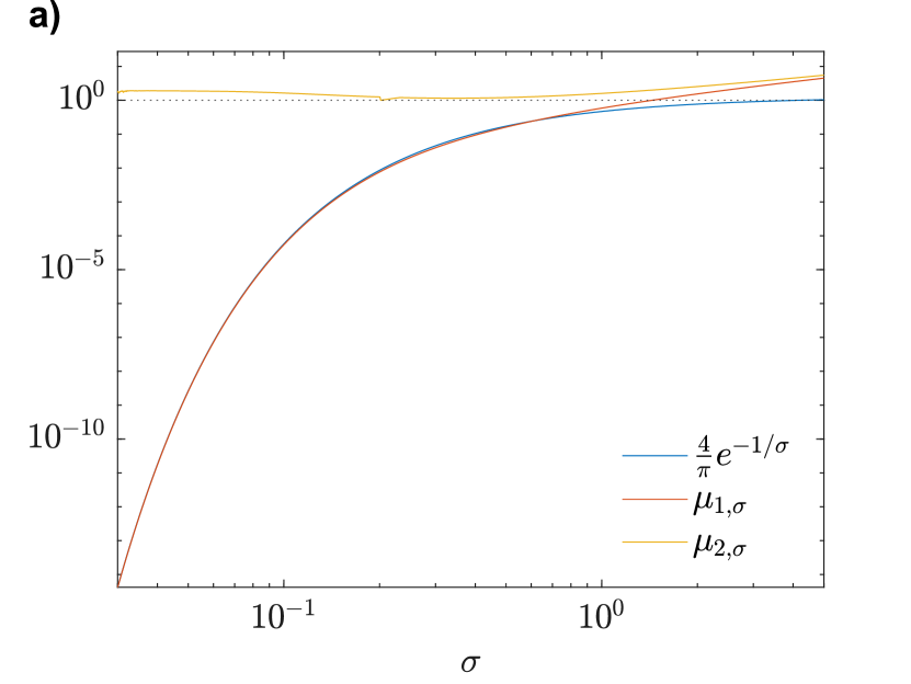
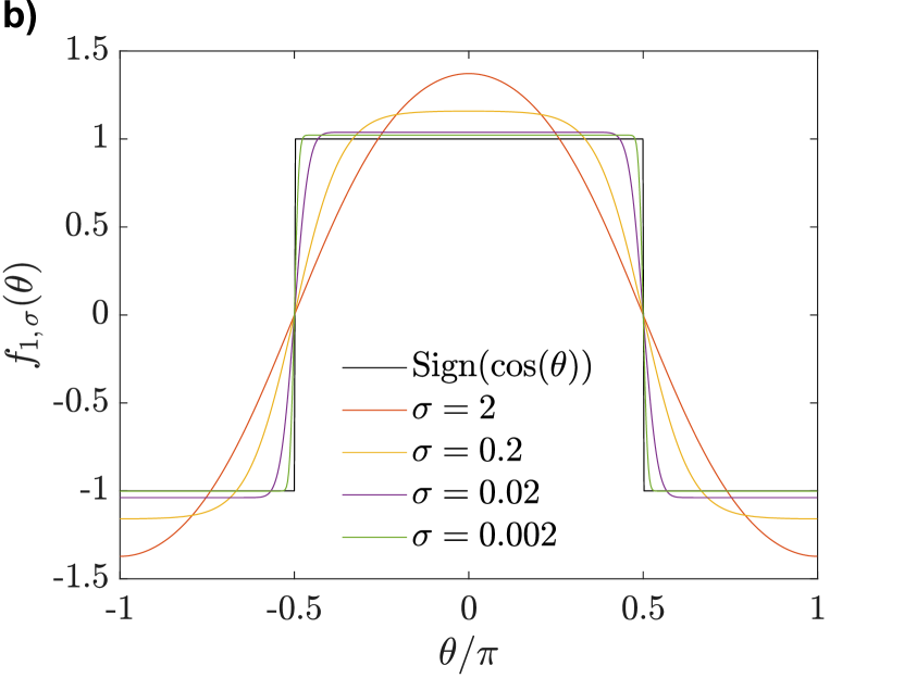
Figure S2: Spectral analysis of $\mathcal{T}_{\sigma}$ for the square GKP code. a) First two non-zero eigenvalues of $\mathcal{T}_{\sigma}$ where $\sigma=\frac{\mathcal{A}\epsilon\eta}{4}=\frac{\epsilon\eta}{4}e^{-\frac{\epsilon\eta}{2}}$. In the limit of small $\sigma$, we observe that the first non-zero eigenvalue $\mu_{1,\sigma}$ is well-approximated by the theoretical asymptotic value $\mu_{1,\sigma}=\frac{4}{\pi}\,e^{-1/\sigma}$ obtained in [87], while the second non-zero eigenvalue $\mu_{2,\sigma}$ is lower-bounded by $1$, opening an exponential spectral gap. b) Numerically computed eigenfunction $f_{1,\sigma}$ associated to the first non-zero eigenvalue $\mu_{1,\sigma}$ for various values of $\sigma$. In the limit of small $\sigma$, we observe that $f_{1,\sigma}(\theta)\rightarrow\operatorname{Sign}(\cos(\theta))$. In both figures, we used $K_{\mathrm{max}}=200$ (corresponding to $2K_{\mathrm{max}}+1=401$ Fourier modes) and numerically checked that higher truncations do not change the results.

S2.1.2 Hexagonal GKP

Let us detail how the eigenvalue analysis led in [87] is generalized to the hexagonal case. Recall from Section S1 the definition of $\eta=2\sqrt{\frac{2\pi}{\sqrt{3}}}$; and the two adapted quadrature operators ${\bf q}_{1}={\bf q},{\bf q}_{2}=\cos(2\pi/3){\bf q}+\sin(2\pi/3){\bf p}=-\tfrac{1}{2}{\bf q}+\tfrac{\sqrt{3}}{2}{\bf p}$, along with the corresponding generalized Pauli operators:

$$\begin{split}{\bf Z}&=\mathrm{Sgn}(\cos(\tfrac{\eta}{2}{\bf q}_{1})),\\ {\bf X}&=\mathrm{Sgn}(\cos(\tfrac{\eta}{2}{\bf q}_{2})),\\ {\bf Y}&=i{\bf Z}{\bf X}\end{split}$$ (S35)

which are indeed products of periodic functions of ${\bf q}_{1}$ and ${\bf q}_{2}$.

In Section S1, we proposed to stabilize a finite-energy hexagonal GKP codespace by engineering a dissipative Lindblad dynamics

$$\frac{d}{dt}\bm{\rho}=\Gamma\,\sum_{k=0}^{5}\mathcal{D}[{\bf L}_{k}](\bm{\rho})$$ (S36)

where $\Gamma>0$, $\epsilon>0$, $\mathcal{A}=e^{-\epsilon\eta/2}$, $\mathcal{D}[{\bf L}](\bm{\rho})={\bf L}\bm{\rho}{\bf L}^{\dagger}-\frac{1}{2}\left({\bf L}^{\dagger}{\bf L}\bm{\rho}+\bm{\rho}{\bf L}^{\dagger}{\bf L}\right)$ and

$${\bf L}_{k}=\mathcal{A}e^{ik\tfrac{\pi}{3}{\bf N}}\,e^{i\eta{\bf q}}\left({\bf 1}-\epsilon{\bf p}\right)\,e^{-ik\tfrac{\pi}{3}{\bf N}}-{\bf 1}.$$ (S37)

Let us now compute the evolution under Eq. S36 of any separable periodic observables of the form

$${\bf h}=h({\bf q}_{1},{\bf q}_{2})=f(\tfrac{\eta}{2}{\bf q}_{1})\,g(\tfrac{\eta}{2}{\bf q}_{2})$$ (S38)

where $f$ and $g$ are real-valued $2\pi$-periodic functions:

$$\frac{d}{dt}\operatorname{Tr}({\bf h}\bm{\rho}_{t}) =\operatorname{Tr}({\bf h}\frac{d}{dt}\bm{\rho}_{t})=\Gamma\sum_{k=0}^{5}\operatorname{Tr}\left({\bf h}\,\mathcal{D}[{\bf L}_{k}](\bm{\rho}_{t})\right)=\Gamma\sum_{k=0}^{5}\operatorname{Tr}\left(\mathcal{D}^{*}[{\bf L}_{k}]({\bf h})\,\bm{\rho}_{t}\right)$$ (S39)

where

$$\mathcal{D}^{*}[{\bf L}_{k}]({\bf h})={\bf L}_{k}^{\dagger}\,{\bf h}\,{\bf L}_{k}-\frac{1}{2}\left({\bf L}_{k}^{\dagger}{\bf L}_{k}\,{\bf h}+{\bf h}\,{\bf L}_{k}^{\dagger}{\bf L}_{k}\right)=\frac{1}{2}\left({\bf L}_{k}^{\dagger}\,[{\bf h},{\bf L}_{k}]+[{\bf L}_{k}^{\dagger},{\bf h}]\,{\bf L}_{k}\right).$$ (S40)

Using the relations of Eq. S9 together with $[{\bf q}_{1},{\bf p}]=i$, $[{\bf q}_{2},{\bf p}]=-\frac{i}{2}$, $[{\bf q}_{1},{\bf q}]~=0$ and $[{\bf q}_{2},{\bf q}]=-\frac{\sqrt{3}}{2}i$, we obtain for instance

$${\bf L}_{0}^{\dagger}\,[{\bf h},{\bf L}_{0}] ={\bf L}_{0}^{\dagger}\,\left[~f(\tfrac{\eta}{2}{\bf q})\,g(\tfrac{\eta}{2}{\bf q}_{2}),\mathcal{A}e^{i\eta{\bf q}}({\bf 1}-\epsilon{\bf p})\right]$$ (S41)

$$=\mathcal{A}\,{\bf L}_{0}^{\dagger}f(\tfrac{\eta}{2}{\bf q})\,\left[g(\tfrac{\eta}{2}{\bf q}_{2}),e^{i\eta{\bf q}}({\bf 1}-\epsilon{\bf p})\right]+\mathcal{A}\,{\bf L}_{0}^{\dagger}\,\left[f(\tfrac{\eta}{2}{\bf q}),e^{i\eta{\bf q}}({\bf 1}-\epsilon{\bf p})\right]\,g(\tfrac{\eta}{2}{\bf q}_{2})$$

$$=-\epsilon\mathcal{A}\,{\bf L}_{0}^{\dagger}\,e^{i\eta{\bf q}}f(\tfrac{\eta}{2}{\bf q})\,\left[g(\tfrac{\eta}{2}{\bf q}_{2}),{\bf p}\right]-\epsilon\mathcal{A}\,{\bf L}_{0}^{\dagger}\,e^{i\eta{\bf q}}\left[f(\tfrac{\eta}{2}{\bf q}),{\bf p}\right]\,g(\tfrac{\eta}{2}{\bf q}_{2})$$

$$=\frac{i\eta\epsilon\mathcal{A}}{4}\,{\bf L}_{0}^{\dagger}\,e^{i\eta{\bf q}}f(\tfrac{\eta}{2}{\bf q})\,g^{\prime}(\tfrac{\eta}{2}{\bf q}_{2})-\frac{i\eta\epsilon\mathcal{A}}{2}\,{\bf L}_{0}^{\dagger}\,e^{i\eta{\bf q}}f^{\prime}(\tfrac{\eta}{2}{\bf q})\,g(\tfrac{\eta}{2}{\bf q}_{2})$$

$$=\frac{i\eta\epsilon\mathcal{A}}{4}\,{\bf L}_{0}^{\dagger}\,e^{i\eta{\bf q}}\left(f(\tfrac{\eta}{2}{\bf q})g^{\prime}(\tfrac{\eta}{2}{\bf q}_{2})\right.\left.-2f^{\prime}(\tfrac{\eta}{2}{\bf q})g(\tfrac{\eta}{2}{\bf q}_{2})\right)$$

$$=\frac{i\eta\epsilon\mathcal{A}}{4}\,\left(\mathcal{A}\left({\bf 1}-\epsilon{\bf p}\right)-e^{i\eta{\bf q}}\right)\left(f(\tfrac{\eta}{2}{\bf q})g^{\prime}(\tfrac{\eta}{2}{\bf q}_{2})\right.\left.-2f^{\prime}(\tfrac{\eta}{2}{\bf q})g(\tfrac{\eta}{2}{\bf q}_{2})\right),$$

$$[{\bf L}_{0}^{\dagger},{\bf h}]\,{\bf L}_{0} =-\frac{i\eta\epsilon\mathcal{A}}{4}\,\left(f(\tfrac{\eta}{2}{\bf q})g^{\prime}(\tfrac{\eta}{2}{\bf q}_{2})\right.\left.-2f^{\prime}(\tfrac{\eta}{2}{\bf q})g(\tfrac{\eta}{2}{\bf q}_{2})\right)\left(\mathcal{A}\left({\bf 1}-\epsilon{\bf p}\right)-e^{-i\eta{\bf q}}\right),$$

$$\mathcal{D}^{*}[{\bf L}_{0}]({\bf h}) =\frac{1}{2}{\bf L}_{0}^{\dagger}\,[{\bf h},{\bf L}_{0}]+\frac{1}{2}[{\bf L}_{0}^{\dagger},{\bf h}]\,{\bf L}_{0}$$ (S42)

$$=-\frac{i\eta\epsilon^{2}\mathcal{A}^{2}}{8}\,\left[{\bf p},f(\tfrac{\eta}{2}{\bf q})g^{\prime}(\tfrac{\eta}{2}{\bf q}_{2})\right.\left.-2f^{\prime}(\tfrac{\eta}{2}{\bf q})g(\tfrac{\eta}{2}{\bf q}_{2})\right]$$

$$\quad\quad\quad-\frac{i\eta\epsilon\mathcal{A}}{8}e^{i\eta{\bf q}}\left(f(\tfrac{\eta}{2}{\bf q})g^{\prime}(\tfrac{\eta}{2}{\bf q}_{2})\right.\left.-2f^{\prime}(\tfrac{\eta}{2}{\bf q})g(\tfrac{\eta}{2}{\bf q}_{2})\right)$$

$$\quad\quad\quad+\frac{i\eta\epsilon\mathcal{A}}{8}\left(f(\tfrac{\eta}{2}{\bf q})g^{\prime}(\tfrac{\eta}{2}{\bf q}_{2})\right.\left.-2f^{\prime}(\tfrac{\eta}{2}{\bf q})g(\tfrac{\eta}{2}{\bf q}_{2})\right)e^{-i\eta{\bf q}}$$

$$=-\frac{\eta^{2}\epsilon^{2}\mathcal{A}^{2}}{8}\,f^{\prime}(\tfrac{\eta}{2}{\bf q})g^{\prime}(\tfrac{\eta}{2}{\bf q}_{2})+\frac{\eta^{2}\epsilon^{2}\mathcal{A}^{2}}{32}\,f(\tfrac{\eta}{2}{\bf q})g^{\prime\prime}(\tfrac{\eta}{2}{\bf q}_{2})+\frac{\eta^{2}\epsilon^{2}\mathcal{A}^{2}}{8}\,f^{\prime\prime}(\tfrac{\eta}{2}{\bf q})g(\tfrac{\eta}{2}{\bf q}_{2})$$

$$\quad\quad\quad-\frac{i\eta\epsilon\mathcal{A}}{8}e^{i\eta{\bf q}}\left(f(\tfrac{\eta}{2}{\bf q})g^{\prime}(\tfrac{\eta}{2}{\bf q}_{2})\right.\left.-2f^{\prime}(\tfrac{\eta}{2}{\bf q})g(\tfrac{\eta}{2}{\bf q}_{2})\right)$$

$$\quad\quad\quad+\frac{i\eta\epsilon\mathcal{A}}{8}\left(f(\tfrac{\eta}{2}{\bf q})g^{\prime}(\tfrac{\eta}{2}{\bf q}_{2})\right.\left.-2f^{\prime}(\tfrac{\eta}{2}{\bf q})g(\tfrac{\eta}{2}{\bf q}_{2})\right)e^{-i\eta{\bf q}}$$

$$=\frac{\eta^{2}\epsilon^{2}\mathcal{A}^{2}}{8}\,\left(f^{\prime\prime}(\tfrac{\eta}{2}{\bf q})g(\tfrac{\eta}{2}{\bf q}_{2})-f^{\prime}(\tfrac{\eta}{2}{\bf q})g^{\prime}(\tfrac{\eta}{2}{\bf q}_{2})+\frac{1}{4}f(\tfrac{\eta}{2}{\bf q})g^{\prime\prime}(\tfrac{\eta}{2}{\bf q}_{2})\right)$$

$$\quad\quad\quad-\frac{i\eta\epsilon\mathcal{A}}{8}e^{i\eta{\bf q}}\left(f(\tfrac{\eta}{2}{\bf q})g^{\prime}(\tfrac{\eta}{2}{\bf q}_{2})\right.\left.-2f^{\prime}(\tfrac{\eta}{2}{\bf q})g(\tfrac{\eta}{2}{\bf q}_{2})\right)$$

$$\quad\quad\quad+\frac{i\eta\epsilon\mathcal{A}}{8}e^{-i\eta{\bf q}}\left(f(\tfrac{\eta}{2}{\bf q})g^{\prime}(\tfrac{\eta}{2}{\bf q}_{2})\right.\left.-2f^{\prime}(\tfrac{\eta}{2}{\bf q})g(\tfrac{\eta}{2}{\bf q}_{2})\right)$$

$$=\frac{\eta^{2}\epsilon^{2}\mathcal{A}^{2}}{8}\,\left(f^{\prime\prime}(\tfrac{\eta}{2}{\bf q})g(\tfrac{\eta}{2}{\bf q}_{2})-f^{\prime}(\tfrac{\eta}{2}{\bf q})g^{\prime}(\tfrac{\eta}{2}{\bf q}_{2})+\frac{1}{4}f(\tfrac{\eta}{2}{\bf q})g^{\prime\prime}(\tfrac{\eta}{2}{\bf q}_{2})\right)$$

$$\quad\quad\quad+\frac{\eta\epsilon\mathcal{A}}{4}\sin(\eta{\bf q})\left(f(\tfrac{\eta}{2}{\bf q})g^{\prime}(\tfrac{\eta}{2}{\bf q}_{2})\right.\left.-2f^{\prime}(\tfrac{\eta}{2}{\bf q})g(\tfrac{\eta}{2}{\bf q}_{2})\right).$$

Applying a $\pi$-rotation in phase-space to the previous expression, we also obtain $\mathcal{D}^{*}[{\bf L}_{3}]({\bf h})=\mathcal{D}^{*}[{\bf L}_{0}]({\bf h})$, so that

$$\mathcal{D}^{*}[{\bf L}_{0}]({\bf h})+\mathcal{D}^{*}[{\bf L}_{3}]({\bf h}) =\frac{\eta^{2}\epsilon^{2}\mathcal{A}^{2}}{4}\,\left(f^{\prime\prime}(\tfrac{\eta}{2}{\bf q})g(\tfrac{\eta}{2}{\bf q}_{2})-f^{\prime}(\tfrac{\eta}{2}{\bf q})g^{\prime}(\tfrac{\eta}{2}{\bf q}_{2})+\frac{1}{4}f(\tfrac{\eta}{2}{\bf q})g^{\prime\prime}(\tfrac{\eta}{2}{\bf q}_{2})\right)$$ (S43)

$$\quad\quad\quad+\frac{\eta\epsilon\mathcal{A}}{2}\sin(\eta{\bf q})\left(f(\tfrac{\eta}{2}{\bf q})g^{\prime}(\tfrac{\eta}{2}{\bf q}_{2})\right.\left.-2f^{\prime}(\tfrac{\eta}{2}{\bf q})g(\tfrac{\eta}{2}{\bf q}_{2})\right).$$

Similar but slightly tedious computations lead to $\mathcal{D}^{*}[{\bf L}_{1}]({\bf h})=\mathcal{D}^{*}[{\bf L}_{4}]({\bf h})$ with

$$\mathcal{D}^{*}[{\bf L}_{1}]({\bf h})+\mathcal{D}^{*}[{\bf L}_{4}]({\bf h}) =\frac{\eta^{2}\epsilon^{2}\mathcal{A}^{2}}{16}\,\left(f^{\prime\prime}(\tfrac{\eta}{2}{\bf q})g(\tfrac{\eta}{2}{\bf q}_{2})+2f^{\prime}(\tfrac{\eta}{2}{\bf q})g^{\prime}(\tfrac{\eta}{2}{\bf q}_{2})+f(\tfrac{\eta}{2}{\bf q})g^{\prime\prime}(\tfrac{\eta}{2}{\bf q}_{2})\phantom{\frac{1}{4}}\right)$$ (S44)

$$\quad\quad\quad-\frac{\eta\epsilon\mathcal{A}}{2}\sin(\eta{\bf q}+\eta{\bf q}_{2})\left(f(\tfrac{\eta}{2}{\bf q})g^{\prime}(\tfrac{\eta}{2}{\bf q}_{2})\right.\left.+f^{\prime}(\tfrac{\eta}{2}{\bf q})g(\tfrac{\eta}{2}{\bf q}_{2})\right),$$

as well as $\mathcal{D}^{*}[{\bf L}_{2}]({\bf h})=\mathcal{D}^{*}[{\bf L}_{5}]({\bf h})$ with

$$\mathcal{D}^{*}[{\bf L}_{2}]({\bf h})+\mathcal{D}^{*}[{\bf L}_{5}]({\bf h}) =\frac{\eta^{2}\epsilon^{2}\mathcal{A}^{2}}{4}\,\left(\frac{1}{4}f^{\prime\prime}(\tfrac{\eta}{2}{\bf q})g(\tfrac{\eta}{2}{\bf q}_{2})-f^{\prime}(\tfrac{\eta}{2}{\bf q})g^{\prime}(\tfrac{\eta}{2}{\bf q}_{2})+f(\tfrac{\eta}{2}{\bf q})g^{\prime\prime}(\tfrac{\eta}{2}{\bf q}_{2})\right)$$ (S45)

$$\quad\quad\quad-\eta\epsilon\mathcal{A}\,\sin(\eta{\bf q}_{2})\left(f(\tfrac{\eta}{2}{\bf q})g^{\prime}(\tfrac{\eta}{2}{\bf q}_{2})\right.\left.-\frac{1}{2}f^{\prime}(\tfrac{\eta}{2}{\bf q})g(\tfrac{\eta}{2}{\bf q}_{2})\right).$$

Finally, we obtain

$$\sum_{k=0}^{5}\mathcal{D}^{*}[{\bf L}_{k}]({\bf h}) =\frac{3\eta^{2}\epsilon^{2}\mathcal{A}^{2}}{8}\,\left(f^{\prime\prime}(\tfrac{\eta}{2}{\bf q})g(\tfrac{\eta}{2}{\bf q}_{2})-f^{\prime}(\tfrac{\eta}{2}{\bf q})g^{\prime}(\tfrac{\eta}{2}{\bf q}_{2})+f(\tfrac{\eta}{2}{\bf q})g^{\prime\prime}(\tfrac{\eta}{2}{\bf q}_{2})\right)$$ (S46)

$$\quad\quad\quad-\eta\epsilon\mathcal{A}\,\left(\sin(\eta{\bf q})+\frac{1}{2}\sin(\eta{\bf q}+\eta{\bf q}_{2})+\frac{1}{2}\sin(\eta{\bf q}_{2})\right)f^{\prime}(\tfrac{\eta}{2}{\bf q})g(\tfrac{\eta}{2}{\bf q}_{2})$$

$$\quad\quad\quad-\eta\epsilon\mathcal{A}\,\left(\sin(\eta{\bf q}_{2})+\frac{1}{2}\sin(\eta{\bf q}+\eta{\bf q}_{2})+\frac{1}{2}\sin(\eta{\bf q})\right)f(\tfrac{\eta}{2}{\bf q})g^{\prime}(\tfrac{\eta}{2}{\bf q}_{2}).$$

We thus obtain the following evolution of ${\bf h}$ in the Heisenberg picture:

$$\Gamma\sum_{k=0}^{5}\mathcal{D}^{*}[{\bf L}_{k}]({\bf h}) =-\mathcal{A}\epsilon\eta\Gamma\,\mathcal{L}_{\sigma}(h)(\tfrac{\eta}{2}{\bf q}_{1},\tfrac{\eta}{2}{\bf q}_{2})$$ (S47)

where $\sigma=\frac{3\mathcal{A}\epsilon\eta}{8}$ and $\mathcal{L}_{\sigma}$ is the differential operator defined by

$$(\mathcal{L}_{\sigma}h)(\theta_{1},\theta_{2})= \,\left(\sin(2\theta_{1})+\frac{1}{2}\sin(2\theta_{1}+2\theta_{2})-\frac{1}{2}\sin(2\theta_{2})\right)\frac{\partial h}{\partial{\theta_{1}}}$$ (S48)

$$+\left(\sin(2\theta_{2})+\frac{1}{2}\sin(2\theta_{1}+2\theta_{2})-\frac{1}{2}\sin(2\theta_{1})\right)\frac{\partial h}{\partial{\theta_{2}}}$$

$$-\sigma\left(\frac{\partial^{2}h}{\partial\theta_{1}^{2}}-\frac{\partial^{2}h}{\partial\theta_{1}\partial\theta_{2}}+\frac{\partial^{2}h}{\partial\theta_{2}^{2}}\right).$$

Here, the crucial difference with the square case is that $\mathcal{L}_{\sigma}$ does not enjoy the nice decomposition of Eq. S20 which allowed us to reduce the study to that of a differential operator in one variable only.

Introducing an adapted scalar product on periodic functions of two variables through

$$\langle f,g\rangle_{\sigma}=\int_{-\pi}^{\pi}\int_{-\pi}^{\pi}e^{-\frac{3-\cos(2\theta_{1})-\cos(2\theta_{1}+2\theta_{2})-\cos(2\theta_{2})}{2\sigma}}\,f(\theta_{1},\theta_{2})^{*}g(\theta_{1},\theta_{2})\,d\theta_{1}d\theta_{2}$$ (S49)

one can check that $\mathcal{L}_{\sigma}$ is self-adjoint for the scalar product $\langle\cdot,\cdot\rangle_{\sigma}$ and non-negative. Indeed, it is a consequence of the following identity, analogous to Eq. S23:

$$w_{\sigma}\mathcal{L}_{\sigma}(f)=-\sigma\,\mathrm{div}(w_{\sigma}A\nabla f)$$ (S50)

where we introduced the matrix

$$A=\begin{bmatrix}1&-1/2\\ -1/2&1\end{bmatrix}$$ (S51)

and a weight function $w_{\sigma}(\theta_{1},\theta_{2})=e^{-\frac{3-\cos(2\theta_{1})-\cos(2\theta_{1}+2\theta_{2})-\cos(2\theta_{2})}{2\sigma}}$ (note that $\langle f,g\rangle_{\sigma}=\int w_{\sigma}f^{*}g$). The differential operator $\mathcal{L}_{\sigma}$ thus has a discrete, real and non-negative spectrum that we can denote in ascending order

$$\lambda_{0,\sigma}\leq\lambda_{1,\sigma}\leq\lambda_{2,\sigma}\leq\ldots$$ (S52)

Of course, for any $\sigma$, the first eigenvalue of $\mathcal{L}_{\sigma}$ still is $\lambda_{0,\sigma}=0$, corresponding to the constant eigenfunction $h\equiv 1$; this simply corresponds to the conservation identity

$$\frac{d}{dt}\operatorname{Tr}(\bm{\rho}_{t})=0.$$

In the limit $\sigma\rightarrow 0$, the other eigenvalues of $\mathcal{L}_{\sigma}$ have also been rigorously studied in [87] (using mathematical results from [89]), where the following asymptotics estimates were obtained:

$$\lambda_{k,\sigma} \sim\frac{12\sqrt{3}}{\pi}e^{-2/\sigma},\quad 1\leq k\leq 3$$ (S53)

$$\lambda_{4,\sigma} \geq\upepsilon_{0}>0$$

where $\upepsilon_{0}$ is a fixed constant independent of $\sigma$. Two remarks are in order when comparing Eq. S53 and the corresponding result in the square case Eq. S33:

• Looking at the exponential dependence on $1/\sigma$ in the first non-zero eigenvalue, one might think at first that we gain a quadratic factor in the hexagonal case. However, one must keep in mind that $\eta$ as well as the definition of $\sigma$ depend on the geometry. For a fixed value of $\epsilon$, we obtain instead a ratio $\frac{2/\sigma_{\mathrm{hexa}}}{1/\sigma_{\mathrm{square}}}\simeq\frac{4}{3}$,

• In the square case, we observed that $\lambda_{1,\sigma}=\lambda_{2,\sigma}=\frac{1}{2}\lambda_{3,\sigma}$; in terms of logical decay rates (see the section about the square case for the link between eigenvalues and logical rates), this meant that the logical ${\bf Y}$ coordinate decayed twice faster than the ${\bf X}$ and ${\bf Z}$ coordinates. This can be related to the fact that the Pauli ${\bf X}$ and ${\bf Z}$ operators correspond to phase-space shifts along the sides of the square grid cell, while ${\bf Y}=-i{\bf Z}{\bf X}$ correspond to a shift along the diagonal, which is longer by a factor $\sqrt{2}$. On the other hand, in the hexagonal case, we get $\lambda_{1,\sigma}=\lambda_{2,\sigma}=\lambda_{3,\sigma}$, reflecting the symmetry of the hexagonal grid. Note that while the above analysis is specific to our dissipation scheme, a similar phenomenon was experimentally observed in [30] where stabilization was achieved using phase estimation of the stabilizers.

Finally, apart from these asymptotic results, we turn to numerical diagonalization of $\mathcal{L}_{\sigma}$ to compute the exact value of $\lambda_{k,\sigma}$ for a fixed value of $\sigma$. To that end, note that $\mathcal{L}_{\sigma}$ also has a simple expression in the Fourier frame: indeed, take $h$ a (smooth) $2\pi$-periodic function of two variables

$$h(\theta_{1},\theta_{2})=\sum_{k_{1},k_{2}\in\mathbb{Z}}h_{k_{1},k_{2}}\,e^{ik_{1}\theta_{1}}e^{ik_{2}\theta_{2}},$$ (S54)

we get

$$(\mathcal{L}_{\sigma}h)(\theta_{1},\theta_{2}) =\left(\sin(2\theta_{1})+\frac{1}{2}\sin(2\theta_{1}+2\theta_{2})-\frac{1}{2}\sin(2\theta_{2})\right)\frac{\partial h}{\partial{\theta_{1}}}$$ (S55)

$$\quad+\left(\sin(2\theta_{2})+\frac{1}{2}\sin(2\theta_{1}+2\theta_{2})-\frac{1}{2}\sin(2\theta_{1})\right)\frac{\partial h}{\partial{\theta_{2}}}$$

$$\quad-\sigma\left(\frac{\partial^{2}h}{\partial\theta_{1}^{2}}-\frac{\partial^{2}h}{\partial\theta_{1}\partial\theta_{2}}+\frac{\partial^{2}h}{\partial\theta_{2}^{2}}\right)$$

$$=\sum_{k_{1},k_{2}\in\mathbb{Z}}\left[\left(ik_{1}\,\frac{e^{2i\theta_{1}}-e^{-2i\theta_{1}}}{2i}+\sigma k_{1}^{2}\right)+\left(ik_{2}\,\frac{e^{2i\theta_{2}}-e^{-2i\theta_{2}}}{2i}+\sigma k_{2}^{2}\right)\right.$$

$$\quad\quad\quad+\left(i\frac{k_{1}+k_{2}}{2}\,\frac{e^{2i\theta_{1}}e^{2i\theta_{2}}-e^{-2i\theta_{1}}e^{-2i\theta_{2}}}{2i}-\sigma k_{1}k_{2}\right)$$

$$\left.\quad\quad\quad-\left(i\frac{k_{1}}{2}\,\frac{e^{2i\theta_{2}}-e^{-2i\theta_{2}}}{2i}+i\frac{k_{2}}{2}\,\frac{e^{2i\theta_{1}}-e^{-2i\theta_{1}}}{2i}\right)\,\right]h_{k_{1},k_{2}}\,e^{ik_{1}\theta_{1}}e^{ik_{2}\theta_{2}}$$

$$=\sum_{k_{1},k_{2}\in\mathbb{Z}}\left[\left(\frac{k_{1}-2}{2}f_{k_{1}-2,k_{2}}-\frac{k_{1}+2}{2}f_{k_{1}+2,k_{2}}+\sigma k_{1}^{2}\,f_{k_{1},k_{2}}\right)\right.$$

$$\quad\quad\quad+\left(\frac{k_{2}-2}{2}f_{k_{1},k_{2}-2}-\frac{k_{2}+2}{2}f_{k_{1},k_{2}+2}+\sigma k_{2}^{2}\,f_{k_{1},k_{2}}\right)$$

$$\quad\quad\quad+\left(\frac{k_{1}+k_{2}-4}{2}f_{k_{1}-2,k_{2}-2}-\frac{k_{1}+k_{2}+4}{2}f_{k_{1}+2,k_{2}+2}+\sigma\,k_{1}k_{2}f_{k_{1},k_{2}}\right)$$

$$\quad\quad\quad+\left.\left(k_{1}\frac{f_{k_{1},k_{2}-2}-f_{k_{1},k_{2}+2}}{2}+k_{2}\frac{f_{k_{1}-2,k_{2}}-f_{k_{1}+2,k_{2}}}{2}\right)\right]e^{ik_{1}\theta_{1}}e^{ik_{2}\theta_{2}}.$$

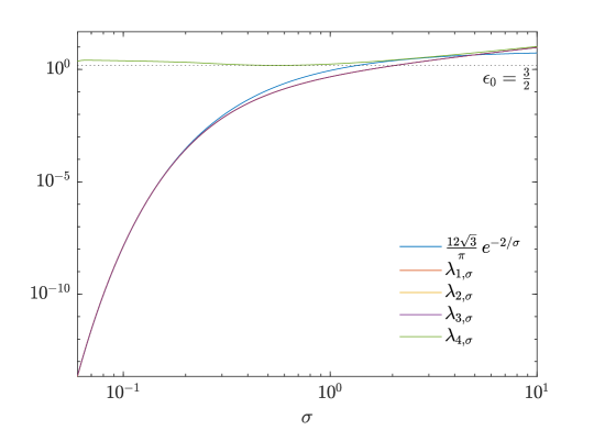
Figure S3: Spectral analysis of $\mathcal{L}_{\sigma}$ for the hexagonal GKP code. First four non-zero eigenvalues of $\mathcal{L}_{\sigma}$. In the limit of small $\sigma$, we observe that the first three (identical) non-zero eigenvalues $\lambda_{k,\sigma},0\leq k\leq 3$ are well-approximated by the theoretical asymptotic value $\lambda_{k,\sigma}=\frac{12\sqrt{3}}{\pi}\,e^{-2/\sigma}$ obtained in [87], while the fourth non-zero eigenvalue $\lambda_{4,\sigma}$ is lower-bounded by $\upepsilon_{0}\simeq 3/2$ (estimated numerically), opening an exponential spectral gap. In this figure, we used $K_{\mathrm{max}}=200$ (corresponding to $(2K_{\mathrm{max}}+1)^{2}=160801$ Fourier modes) and numerically checked that higher truncations do not change the results.

In the Fourier frame, $\mathcal{L}_{\sigma}$ can thus be approximated by truncating the sum above to $-K_{\textrm{max}}\leq k_{1},k_{2}\leq K_{\textrm{max}}$ (i.e. bounding the maximum frequency considered). On Fig. S3 we compare the numerical eigenvalues obtained by this procedure to the explicit asymptotic expressions of Eq. S53. The analysis led at the end of Section S2.1.1 to explain, in the square case, the interpretation of the eigenvalues of $\mathcal{L}_{\sigma}$ in terms of logical decoherence rates can be adapted straightforwardly to the hexagonal case.

S2.1.3 Protection against quadrature noise

In presence of quadrature noise, the previous exact eigenvalue analysis can be adapted by adding the contribution of dissipators along the two quadrature operators ${\bf q}$ and ${\bf p}$. More precisely, for a given separable periodic observable ${\bf h}=h(\tfrac{\eta}{2}{\bf q}_{1},\tfrac{\eta}{2}{\bf q}_{2})=f(\tfrac{\eta}{2}{\bf q}_{1})\,g(\tfrac{\eta}{2}{\bf q}_{2})$ we have to compute

$$\frac{d}{dt}\operatorname{Tr}\Big{(}{\bf h}\big{(}\kappa\mathcal{D}[{\bf q}](\bm{\rho}_{t})+\kappa\mathcal{D}[{\bf p}](\bm{\rho}_{t})\big{)}\Big{)}=\kappa\operatorname{Tr}\left(\mathcal{D}^{*}[{\bf q}]({\bf h})\bm{\rho}_{t}\right)+\kappa\operatorname{Tr}\left(\mathcal{D}^{*}[{\bf p}]({\bf h})\bm{\rho}_{t}\right).$$ (S56)

Square GKP.

For a square GKP grid, we have $\eta=2\sqrt{\pi}$, ${\bf q}_{1}={\bf q}$, ${\bf q}_{2}={\bf p}$. Using similar computations (see [87]) we get

$$\mathcal{D}^{*}[{\bf q}]({\bf h}) =\frac{\eta^{2}}{8}f(\tfrac{\eta}{2}{\bf q})\,g^{\prime\prime}(\tfrac{\eta}{2}{\bf p})$$ (S57)

$$\mathcal{D}^{*}[{\bf p}]({\bf h}) =\frac{\eta^{2}}{8}f^{\prime\prime}(\tfrac{\eta}{2}{\bf q})\,g(\tfrac{\eta}{2}{\bf p}).$$ (S58)

Note that these terms already appeared in Eq. S19 so that putting everything together we obtain

$$\Gamma\sum_{k=0}^{3}\mathcal{D}^{*}[{\bf L}_{k}]({\bf h})+\kappa\left(\mathcal{D}^{*}[{\bf q}]({\bf h})+\mathcal{D}^{*}[{\bf p}]({\bf h})\right)= -\mathcal{A}\epsilon\eta\Gamma\,\left(\sin(\eta{\bf q})f^{\prime}(\tfrac{\eta}{2}{\bf q})-\left(\frac{\mathcal{A}\epsilon\eta}{4}+\frac{\kappa\eta}{8\mathcal{A}\epsilon\Gamma}\right)f^{\prime\prime}(\tfrac{\eta}{2}{\bf q})\right)g(\tfrac{\eta}{2}{\bf p})$$ (S59)

$$-\mathcal{A}\epsilon\eta\Gamma\,f(\tfrac{\eta}{2}{\bf q})\left(\sin(\eta{\bf p})g^{\prime}(\tfrac{\eta}{2}{\bf p})-\left(\frac{\mathcal{A}\epsilon\eta}{4}+\frac{\kappa\eta}{8\mathcal{A}\epsilon\Gamma}\right)g^{\prime\prime}(\tfrac{\eta}{2}{\bf p})\right)$$

$$= -\mathcal{A}\epsilon\eta\Gamma\,\mathcal{L}_{\sigma}(h)(\tfrac{\eta}{2}{\bf q},\tfrac{\eta}{2}{\bf p})$$

where the differential operator $\mathcal{L}_{\sigma}$ is still defined by Eq. S20 but its parameter $\sigma$ now also depends on $\kappa/\Gamma$ through

$$\sigma=\frac{\mathcal{A}\epsilon\eta}{4}+\frac{\kappa\eta}{8\mathcal{A}\epsilon\Gamma}.$$ (S60)

As a consequence, we emphasize that in presence of quadrature noise, the optimal choice of energy truncation no longer consists in minimizing $\epsilon$. Indeed, in the regime $\sigma\ll 1$, the logical decoherence rate is given by

$$\Gamma_{L}=\mathcal{A}\epsilon\eta\Gamma\,\lambda_{1,\sigma}\simeq\frac{4}{\pi}\mathcal{A}\epsilon\eta\Gamma\,e^{-1/{\sigma}}=\frac{4}{\pi}\mathcal{A}\epsilon\eta\Gamma\,e^{-\left(\frac{\mathcal{A}\epsilon\eta}{4}+\frac{\kappa\eta}{8\mathcal{A}\epsilon\Gamma}\right)^{-1}}.$$ (S61)

At leading order in $\kappa/\Gamma$, this value is minimized for an optimal choice of $\epsilon$ given by

$$\epsilon^{\star}=\sqrt{\frac{\kappa}{2\mathcal{A}^{2}\Gamma}}$$ (S62)

(if desired, one could refine this value by computing the next coefficients of the asymptotic expansion of $\epsilon^{\star}$ in powers of $\sqrt{\frac{\kappa}{\Gamma}}$). Using Eq. S61, the corresponding logical decoherence rate is

$$\Gamma^{\star}_{L}\simeq\frac{4\eta}{\pi}\,\sqrt{\frac{\kappa\Gamma}{2}}\,e^{-\frac{2}{\eta}\sqrt{\frac{2\Gamma}{\kappa}}}.$$ (S63)

We emphasize that the asymptotic expression of $\Gamma_{L}$ given by Eq. S61 is only valid in the regime $\sigma\rightarrow 0$. In particular, it cannot be used to estimate the decoherence rate when $\epsilon\rightarrow 0$ for a fixed value of $\kappa$, as in that case $\sigma\rightarrow+\infty$. In that opposite regime, the first non-zero eigenvalue $\lambda_{1,\sigma}$ of $\mathcal{L}_{\sigma}$ satisfies $\lambda_{1,\sigma}\simeq\sigma$ so that the corresponding logical decoherence rate is given, at first order, by

$$\Gamma_{L}^{\epsilon\rightarrow 0}\simeq\mathcal{A}\epsilon\eta\Gamma\sigma\simeq\frac{\kappa\eta^{2}}{8}.$$ (S64)

This decoherence rate is linear in $\kappa$ so that the effect of the stabilization is entirely lost: the logical decoherence rate is trivially piloted by the strength of the quadrature noise.

Hexagonal GKP.

For a hexagonal GKP grid, we have $\eta=2\sqrt{\frac{2\pi}{\sqrt{3}}}$, ${\bf q}_{1}={\bf q}$, ${\bf q}_{2}=\cos(\frac{2\pi}{3}){\bf q}+\sin(\frac{2\pi}{3}){\bf p}=-\frac{1}{2}{\bf q}+\frac{\sqrt{3}}{2}{\bf p}$, and in particular $[{\bf q},{\bf q}_{1}]=0$, $[{\bf q},{\bf q}_{2}]=\frac{\sqrt{3}}{2}i$, $[{\bf p},{\bf q}_{1}]=-i$, $[{\bf p},{\bf q}_{2}]=\frac{i}{2}$. We thus get

$$\mathcal{D}^{*}[{\bf q}]({\bf h}) =\frac{1}{2}{\bf q}[{\bf h},{\bf q}]+\frac{1}{2}[{\bf q},{\bf h}]{\bf q}$$ (S65)

$$=\frac{1}{2}{\bf q}\,f(\tfrac{\eta}{2}{\bf q})[g(\tfrac{\eta}{2}{\bf q}_{2}),{\bf q}]+\frac{1}{2}f(\tfrac{\eta}{2}{\bf q})[{\bf q},g(\tfrac{\eta}{2}{\bf q}_{2})]\,{\bf q}$$

$$=-\frac{i\eta\sqrt{3}}{8}{\bf q}\,f(\tfrac{\eta}{2}{\bf q})g^{\prime}(\tfrac{\eta}{2}{\bf q}_{2})+\frac{i\eta\sqrt{3}}{8}f(\tfrac{\eta}{2}{\bf q})g^{\prime}(\tfrac{\eta}{2}{\bf q}_{2})\,{\bf q}$$

$$=\frac{i\eta\sqrt{3}}{8}f(\tfrac{\eta}{2}{\bf q})[g^{\prime}(\tfrac{\eta}{2}{\bf q}_{2}),{\bf q}]$$

$$=\frac{3\eta^{2}}{32}f(\tfrac{\eta}{2}{\bf q})g^{\prime\prime}(\tfrac{\eta}{2}{\bf q}_{2})$$

and

$$\mathcal{D}^{*}[{\bf p}]({\bf h}) =\frac{1}{2}{\bf p}[{\bf h},{\bf p}]+\frac{1}{2}[{\bf p},{\bf h}]{\bf p}$$ (S66)

$$=\frac{1}{2}{\bf p}\,[f(\tfrac{\eta}{2}{\bf q}),{\bf p}]\,g(\tfrac{\eta}{2}{\bf q}_{2})+\frac{1}{2}[{\bf p},f(\tfrac{\eta}{2}{\bf q})]\,g(\tfrac{\eta}{2}{\bf q}_{2}){\bf p}+\frac{1}{2}{\bf p}f(\tfrac{\eta}{2}{\bf q})\,[g(\tfrac{\eta}{2}{\bf q}_{2}),{\bf p}]+\frac{1}{2}f(\tfrac{\eta}{2}{\bf q})\,[{\bf p},g(\tfrac{\eta}{2}{\bf q}_{2})]{\bf p}$$

$$=\frac{i\eta}{4}{\bf p}\,f^{\prime}(\tfrac{\eta}{2}{\bf q})g(\tfrac{\eta}{2}{\bf q}_{2})-\frac{i\eta}{4}f^{\prime}(\tfrac{\eta}{2}{\bf q})g(\tfrac{\eta}{2}{\bf q}_{2}){\bf p}-\frac{i\eta}{8}{\bf p}f(\tfrac{\eta}{2}{\bf q})g^{\prime}(\tfrac{\eta}{2}{\bf q}_{2})+\frac{i\eta}{8}f(\tfrac{\eta}{2}{\bf q})g^{\prime}(\tfrac{\eta}{2}{\bf q}_{2}){\bf p}$$

$$=\frac{i\eta}{4}[{\bf p},f^{\prime}(\tfrac{\eta}{2}{\bf q})g(\tfrac{\eta}{2}{\bf q}_{2})]-\frac{i\eta}{8}[{\bf p},f(\tfrac{\eta}{2}{\bf q})g^{\prime}(\tfrac{\eta}{2}{\bf q}_{2})]$$

$$=\frac{i\eta}{4}f^{\prime}(\tfrac{\eta}{2}{\bf q})\,[{\bf p},g(\tfrac{\eta}{2}{\bf q}_{2})]-\frac{i\eta}{8}f(\tfrac{\eta}{2}{\bf q})\,[{\bf p},g^{\prime}(\tfrac{\eta}{2}{\bf q}_{2})]+\frac{i\eta}{4}[{\bf p},f^{\prime}(\tfrac{\eta}{2}{\bf q})]\,g(\tfrac{\eta}{2}{\bf q}_{2})]-\frac{i\eta}{8}[{\bf p},f(\tfrac{\eta}{2}{\bf q})]\,g^{\prime}(\tfrac{\eta}{2}{\bf q}_{2})]$$

$$=-\frac{\eta^{2}}{8}f^{\prime}(\tfrac{\eta}{2}{\bf q})g^{\prime}(\tfrac{\eta}{2}{\bf q}_{2})+\frac{\eta^{2}}{32}f(\tfrac{\eta}{2}{\bf q})g^{\prime\prime}(\tfrac{\eta}{2}{\bf q}_{2})+\frac{\eta^{2}}{8}f^{\prime\prime}(\tfrac{\eta}{2}{\bf q})g(\tfrac{\eta}{2}{\bf q}_{2})$$

so that

$$\mathcal{D}^{*}[{\bf q}]({\bf h})+\mathcal{D}^{*}[{\bf p}]({\bf h}) =\frac{\eta^{2}}{8}\Big{(}f^{\prime\prime}(\tfrac{\eta}{2}{\bf q})g(\tfrac{\eta}{2}{\bf q}_{2})-f^{\prime}(\tfrac{\eta}{2}{\bf q})g^{\prime}(\tfrac{\eta}{2}{\bf q}_{2})+f(\tfrac{\eta}{2}{\bf q})g^{\prime\prime}(\tfrac{\eta}{2}{\bf q}_{2})\Big{)}$$ (S67)

$$=\frac{\eta^{2}}{8}\Big{(}\frac{\partial^{2}h}{\partial\theta_{1}^{2}}-\frac{\partial^{2}h}{\partial\theta_{1}\partial\theta_{2}}+\frac{\partial^{2}h}{\partial\theta_{2}^{2}}\Big{)}({\bf q}_{1},{\bf q}_{2}).$$

Note that these terms already appeared in Eq. S47 so that putting everything together we obtain

$$\Gamma\sum_{k=0}^{5}\mathcal{D}^{*}[{\bf L}_{k}]({\bf h})+\kappa\left(\mathcal{D}^{*}[{\bf q}]({\bf h})+\mathcal{D}^{*}[{\bf p}]({\bf h})\right)= -\mathcal{A}\epsilon\eta\Gamma\,\mathcal{L}_{\sigma}(h)(\tfrac{\eta}{2}{\bf q}_{1},\tfrac{\eta}{2}{\bf q}_{2})$$ (S68)

where the differential operator $\mathcal{L}_{\sigma}$ is still defined by Eq. S48 but its parameter $\sigma$ now also depends on $\kappa/\Gamma$ through

$$\sigma=\frac{3\mathcal{A}\epsilon\eta}{8}+\frac{\kappa\eta}{8\mathcal{A}\epsilon\Gamma}.$$ (S69)

Once again, this entails that there is an optimal choice of energy truncation in presence of quadrature noise, approximately corresponding to

$$\epsilon^{\star}=\sqrt{\frac{\kappa}{3\mathcal{A}^{2}\Gamma}}.$$ (S70)

The corresponding logical decoherence rate is

$$\Gamma^{\star}=\frac{12\eta}{\pi}\sqrt{\kappa\Gamma}\,e^{-\frac{8}{3\eta}\sqrt{\frac{3\Gamma}{\kappa}}}.$$ (S71)

S2.2 Explicit energy estimates

In Section S2.1, we analyzed the evolution of periodic operators in the Heisenberg picture. To support the claim that the dissipation stabilizes finite-energy grid states, we also need to verify that energy is bounded under this dissipative dynamics. To this end, we showed in a separate publication that one can compute explicit bounds on the energy (average photon number) $\langle{\bf N}\rangle=\operatorname{Tr}({\bf N}\bm{\rho})$ along trajectories of a quantum system stabilized by the modular dissipators proposed above; in this subsection, we recall and gather the results obtained in [87]. When performing numerical dynamical simulations in the Fock basis, such energy estimates give a rationale for choosing an adapted truncation.

For any integer $M\geq 1$, let us introduce the generalized family of $2M$ Lindblad operators defined by

$${\bf L}_{k}=e^{i\theta_{k}{\bf N}}\,\left(\mathcal{A}e^{i\eta{\bf q}}\left({\bf 1}-\epsilon{\bf p}\right)-{\bf 1}\right)e^{-i\theta_{k}{\bf N}},\quad\quad 0\leq k\leq 2M-1$$ (S72)

where $\theta_{k}=\frac{ik\pi}{M}$ and $\mathcal{A}=e^{-\eta\epsilon/2}$. For $M=2$, we find the four Lindblad operators used to stabilize a square GKP code, while for $M=3$, we find the six Lindblad operators used to stabilize a hexagonal GKP code.
We have the following energy estimate:

Estimate 1.

Assume that $\operatorname{Tr}({\bf N}\bm{\rho}_{0})<+\infty$, $\epsilon\eta/2<0.4$ and the evolution of $\bm{\rho}_{t}$ is governed by the Lindblad equation

$$\begin{split}\frac{\mathrm{d}\bm{\rho}_{t}}{\mathrm{d}t}&=\sum^{2M-1}_{k=0}\Gamma\mathcal{D}[{\bf L}_{k}]\bm{\rho}_{t}=\sum^{2M-1}_{k=0}\Gamma\big{(}{\bf L}_{k}\bm{\rho}_{t}{\bf L}_{k}^{\dagger}-\frac{1}{2}({\bf L}_{k}^{\dagger}{\bf L}_{k}\bm{\rho}_{t}+\bm{\rho}_{t}{\bf L}_{k}^{\dagger}{\bf L}_{k})\big{)}.\end{split}$$ (S73)

Then, for all $t\geq 0$ :

$$\begin{split}\operatorname{Tr}({\bf N}\bm{\rho}_{t})&\leq\,e^{-\lambda(\epsilon,\eta)t}\operatorname{Tr}({\bf N}\bm{\rho}_{0})+\left(1-e^{-\lambda(\epsilon,\eta)t}\right)C(\epsilon,\eta).\end{split}$$ (S74)

where $\lambda(\epsilon,\eta)$ and $C(\epsilon,\eta)$ are positive constants defined in [87], which satisfy the following asymptotics when $\epsilon\rightarrow 0^{+}$:

$$\begin{split}\lambda(\epsilon,\eta)&\sim 2\,M\Gamma\,\epsilon\eta,\\ C(\epsilon,\eta)&\sim\frac{\eta}{2\epsilon}.\end{split}$$ (S75)

We emphasize that the puzzling hypothesis $\epsilon\eta/2<0.4$ is only a sufficient condition to ensure $((2-\epsilon\eta/2)\mathcal{A}-1)>0$ and can be safely mentally replaced by for small enough $\epsilon$ while reading the proof. In particular, it is satisfied in every numerical simulation presented here. As a consequence of this estimate, any solution starting from an initial state satisfying $\operatorname{Tr}({\bf N}\bm{\rho}_{0})\leq C(\epsilon,\eta)$ satisfies $\operatorname{Tr}({\bf N}\bm{\rho}_{t})\leq C(\epsilon,\eta)$ along the whole trajectory.

Finally, note that, while the previous computations are valid for any value of $M$, the only choices allowing the resulting dynamics to stabilize a logical qubit are $M=2$ (corresponding to a square grid) and $M=3$ (corresponding to a hexagonal grid).

The full proof of 1 can be found in [87]. Let us only recall one core idea of the proof, which will also prove instrumental in Section S2.3 to understand the instability of other possible candidate dynamics for the stabilization of GKP qubits.

Using the definition of the operators ${\bf L}_{k}$, we compute the evolution of ${\bf N}$ as

$$\begin{split}\frac{d}{dt}\operatorname{Tr}({\bf N}\bm{\rho}_{t})&=\sum_{k=0}^{2M-1}\Gamma\operatorname{Tr}(\mathcal{D}^{*}[{\bf L}_{k}]({\bf N})\bm{\rho}_{t})=\sum_{k=0}^{2M-1}\Gamma\,\operatorname{Tr}(e^{\frac{ik\pi}{M}{\bf N}}\,\mathcal{D}^{*}[{\bf L}_{0}]({\bf N})\,e^{-\frac{ik\pi}{M}{\bf N}}\bm{\rho}_{t})\quad\end{split}$$ (S76)

where

$$\begin{split}\mathcal{D}^{*}[{\bf L}_{0}]({\bf N})&:={\bf L}_{0}^{\dagger}{\bf N}{\bf L}_{0}-\frac{1}{2}\left({\bf L}_{0}^{\dagger}{\bf L}_{0}{\bf N}+{\bf N}{\bf L}_{0}^{\dagger}{\bf L}_{0}\right)=\frac{1}{2}\left({\bf L}_{0}^{\dagger}\big{[}{\bf N},{\bf L}_{0}\big{]}+\big{[}{\bf N},{\bf L}_{0}^{\dagger}\big{]}{\bf L}_{0}\right)=\frac{1}{2}\,{\bf L}_{0}^{\dagger}\left[{\bf N},{\bf L}_{0}\right]+\operatorname{h.c.}\end{split}$$ (S77)

We can then show [87] that

$$\mathcal{D}^{*}[{\bf L}_{0}]({\bf N}) =\epsilon^{2}\eta\mathcal{A}^{2}{\bf p}^{3}$$

$$\quad+\frac{\epsilon^{2}+\eta^{2}}{2}\mathcal{A}^{2}{\bf 1}+\eta(1-\epsilon\eta)\mathcal{A}^{2}{\bf p}-\epsilon\eta(2-\frac{\epsilon\eta}{2})\mathcal{A}^{2}{\bf p}^{2}+\frac{\epsilon\eta^{3}}{4}\mathcal{A}\cos(\eta{\bf q})-\epsilon\mathcal{A}{\bf q}\sin(\eta{\bf q})$$

$$\quad-\eta(1+\frac{\epsilon\eta}{2})\mathcal{A}\cos(\eta{\bf q}){\bf p}-i\frac{\eta^{2}}{4}(2+\epsilon\eta)\mathcal{A}\sin(\eta{\bf q})+\epsilon\eta\mathcal{A}\,{\bf p}\cos(\eta{\bf q}){\bf p}.$$ (S78)

Crucially, the ominous cubic leading term, that could lead to instability, cancels out when we sum the contributions of all the dissipators in Eq. S76, as each Lindblad operator is paired to its image by a $\pi$ rotation in phase-space. The leading coefficient of the next quadratic term is negative, which allows us to recover the desired stability property.

S2.3 Instability of a dynamics enforced by two dissipators

As explained in Section V, realizing an effective Lindblad dynamics with several engineered dissipators can be done either by coupling the target mode to as many ancillary modes as there are dissipators to engineer, or by resorting to a Trotterization procedure where one activates sequentially each dissipator. In the first case, the complexity of the experiment is proportional to the number of dissipators to engineer. In the second case, the achievable engineered dissipation rate $\Gamma$ is inversely proportional to that number. It is thus natural to wonder whether the dynamics we propose, featuring respectively four dissipators for the stabilization of square GKP states and six dissipators for the stabilization of hexagonal GKP states, are optimal in the number of dissipators to engineer. For the remaining of this section, we will focus on the square GKP case; our arguments are straightforwardly adapted to the hexagonal case. We examine several ideas for the stabilization of the square GKP codespace using only two dissipators, and find that each of them leads to instable dynamical behavior.

S2.3.1 Candidate dynamics

Recall from Section II that the infinite-energy square GKP codespace can be defined as the common +1-eigenspace of the two stabilizer operators ${\bf S}_{q}=e^{i\eta{\bf q}}$ and ${\bf S}_{p}=e^{-i\eta{\bf p}}$ which correspond to shift operators in phase space. Similarly, the finite-energy square GKP codespace can be defined as the common +1-eigenspace of the two stabilizer operators ${\bf S}_{q}^{\Delta}=e^{-\Delta{\bf a}^{\dagger}{\bf a}}\,{\bf S}_{q}\,e^{\Delta{\bf a}^{\dagger}{\bf a}}$ and ${\bf S}_{p}^{\Delta}=e^{-\Delta{\bf a}^{\dagger}{\bf a}}\,{\bf S}_{p}\,e^{\Delta{\bf a}^{\dagger}{\bf a}}$. The stabilizing dynamics we introduced in Section III reads

$$\frac{d\bm{\rho}_{t}}{dt}:=\mathcal{L}_{4}(\bm{\rho}_{t})=\Gamma\sum_{k=0}^{3}\mathcal{D}[{\bf L}_{k}](\bm{\rho}_{t}),$$ (S79)

where the four Lindblad operators

$${\bf L}_{k}=\mathcal{A}{\bf R}_{\frac{k\pi}{2}}\,e^{i\eta{\bf q}}(1-\epsilon{\bf p})\,{\bf R}_{\frac{k\pi}{2}}^{\dagger}-{\bf 1},\quad 0\leq k\leq 3,\quad\epsilon=\eta~\sinh(\Delta)$$

correspond to first order approximations of ${\bf S}_{q}^{\Delta}-{\bf 1}$, ${\bf S}_{p}^{\Delta}-{\bf 1}$ as well as their image by a $\pi$ rotation in phase-space. This rotation in phase-space can be understood as initially adding the two adjoint stabilizer operators ${\bf S}_{q}^{\dagger}=e^{-i\eta{\bf q}}$ and ${\bf S}_{p}^{\dagger}=e^{i\eta{\bf p}}$ in the definition of the GKP codespace, which seems redundant. It is thus tempting to think that only the two first dissipators are required, and that one could engineer the simpler candidate Lindblad dynamics

$$\frac{d\bm{\rho}_{t}}{dt}:=\mathcal{L}_{2}(\bm{\rho}_{t})=\Gamma\big{(}\mathcal{D}[{\bf L}_{0}](\bm{\rho}_{t})+\mathcal{D}[{\bf L}_{1}](\bm{\rho}_{t})\big{)}.$$ (S80)

A related idea would be to consider instead the symmetric sums of Lindblad operators

$${\bf L}_{q,s} =({\bf L}_{0}+{\bf L}_{2})/\sqrt{2}=\sqrt{2}\big{(}\mathcal{A}\left(\cos(\eta{\bf q})-i\epsilon\sin(\eta{\bf q}){\bf p}\right)-{\bf 1}~\big{)}$$

$${\bf L}_{p,s} =({\bf L}_{1}+{\bf L}_{3})/\sqrt{2}=\sqrt{2}\big{(}\mathcal{A}\left(\cos(\eta{\bf p})+i\epsilon\sin(\eta{\bf p}){\bf q}\right)-{\bf 1}~\big{)},$$

which amounts to defining the GKP codespace through the stabilizers $\cos(\eta{\bf q})$ and $\cos(\eta{\bf p})$ instead of $e^{i\eta{\bf q}}$ and $e^{-i\eta{\bf p}}$. Another candidate Lindblad dynamics with only two dissipators is thus

$$\frac{d\bm{\rho}_{t}}{dt}:=\mathcal{L}_{2,s}(\bm{\rho}_{t})=\Gamma\big{(}\mathcal{D}[{\bf L}_{q,s}](\bm{\rho}_{t})+\mathcal{D}[{\bf L}_{p,s}](\bm{\rho}_{t})\big{)}.$$ (S81)

Finally, we note that another Lindblad dynamics with two dissipators was proposed in [29]:

$$\frac{d\bm{\rho}_{t}}{dt}:=\mathcal{L}_{2,\log{}}(\bm{\rho}_{t})=\Gamma\big{(}\mathcal{D}[{\bf L}_{0,\log{}}](\bm{\rho}_{t})+\mathcal{D}[{\bf L}_{1,\log{}}](\bm{\rho}_{t})\big{)}$$ (S82)

where

$${\bf L}_{0,\log{}} =-\frac{i}{2\sqrt{\pi\cosh(\Delta)\sinh(\Delta)}}\log({\bf S}_{q}^{\Delta})=\frac{{\bf q}_{[m]}}{\sqrt{2\tanh(\Delta)}}+i{\bf p}\sqrt{\frac{\tanh(\Delta)}{2}}$$

$${\bf L}_{1,\log{}} =-\frac{i}{2\sqrt{\pi\cosh(\Delta)\sinh(\Delta)}}\log({\bf S}_{p}^{\Delta})=\frac{{\bf p}_{[m]}}{\sqrt{2\tanh(\Delta)}}-i{\bf q}\sqrt{\frac{\tanh(\Delta)}{2}}$$

where $m=\frac{2\pi}{\eta\cosh(\Delta)}$ and ${\bf q}_{[m]}={\bf q}\mod m$, ${\bf p}_{[m]}={\bf p}\mod m$ are modular quadrature operators. This choice of dissipators can be intuitively understood as such: to build a Lindblad operator that cancels on the codespace, given a stabilizer operator ${\bf S}$, the authors use $\log({\bf S})$ instead of ${\bf S}-{\bf 1}$. Note that, while the strategy presented in the main text to engineer the dynamics $\mathcal{L}_{4}$ would also be immediately suitable for the engineering of the two candidate dynamics $\mathcal{L}_{2}$ and $\mathcal{L}_{2,s}$, there is currently no clear way to engineer the dynamics $\mathcal{L}_{2,\log{}}$. For this reason, we focus mainly on the analysis of $\mathcal{L}_{2}$ and $\mathcal{L}_{2,s}$, but still included $\mathcal{L}_{2,\log}$ in our numerical comparisons to assess its theoretical merits.

S2.3.2 Numerical study of the stability

To detect potential dynamical instabilities, we numerically simulate the evolution of a density operator $\bm{\rho}_{t}$ initialized in vacuum ($\bm{\rho}_{0}=|0\rangle\langle 0|$). The exact choice of initial state is arbitrary: in order to ease the detection of instabilities, one should preferably choose an initial state far from the codespace (as states in the codespace would be metastable states of any reasonable candidate dynamics).

On Fig. S4, we plot the evolution of the mean photon number $\langle{\bf N}\rangle(t)=\operatorname{Tr}({\bf N}\bm{\rho}_{t})$ for the four studied dynamics: $\mathcal{L}_{4},\mathcal{L}_{2},\mathcal{L}_{2,s}$ and $\mathcal{L}_{2,\log}$. Using the stability results obtained in Section S2.2, we already know that the mean photon number remains bounded when $\bm{\rho}_{t}$ is governed by the four dissipators dynamics $\mathcal{L}_{4}$, where the exact bound depends on the maximum between the initial energy and a fixed constant depending only on $\epsilon$ and $\Gamma$; this result is verified numerically. On the other hand, when $\bm{\rho}_{t}$ is evolved with $\mathcal{L}_{2}$ and $\mathcal{L}_{2,s}$, the mean photon number grows well beyond its value in the codespace. We emphasize that one should not conclude that this energy still stays bounded, only with a higher bound: in fact, we observe that the maximum value grows when increasing the necessary truncation of the Hilbert space used in simulation, from which one can only conclude that the true trajectory is unbounded. Finally, when $\bm{\rho}_{t}$ is evolved with $\mathcal{L}_{2,\log}$, the mean photon number features an initial bump, before eventually decreasing to a value close to the one observed with $\mathcal{L}_{4}$. However, once again, we observe that the height of the initial bump increases with the truncation of the Hilbert space, suggesting that this dynamics is also instable and merely artificially constrained by the numerical truncation.

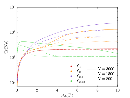
Figure S4: Instability of the candidates two-dissipators dynamics. For each proposed dynamics, we plot the evolution of the average photon number $\langle{\bf N}\rangle(t)=\operatorname{Tr}({\bf N}\bm{\rho}_{t})$ when the system is initialized in $\bm{\rho}_{0}=|0\rangle\langle 0|$. The dynamics $\mathcal{L}_{4}$ corresponds to the four-dissipators Lindblad equation we propose for the stabilization of the square GKP codespace. The three other dynamics $\mathcal{L}_{2},\mathcal{L}_{2,s}$ and $\mathcal{L}_{2,\log}$ correspond to the candidate two-dissipators dynamics introduced in the current section. Here, we chose a parameter $\epsilon=0.15$ and the numerical simulations are performed in a Hilbert space truncated to the first $N$ Fock states, with respectively $N=800$ (dotted lines), $N=1500$ (dashed lines) and $N=3000$ (full lines). We observe that the curves associated to $\mathcal{L}_{2},\mathcal{L}_{2,s}$ and $\mathcal{L}_{2,\log}$ do not seem to converge even at these rather high truncation numbers, and that their maximal value actually increases with the truncation. This phenomenon hints at the intrinsic instability of these three dynamics, that only seem bounded for a given truncation due to the effects of the truncation itself.

S2.3.3 Qualitative understanding

In addition to the formal stability result of Section S2.2, we can propose more qualitative insight into the stability of $\mathcal{L}_{4}$ and the instability of the other dynamics, especially $\mathcal{L}_{2}$ and $\mathcal{L}_{2,s}$.

In general, when considering any time-independent Lindblad equation of the form

$$\frac{d\bm{\rho}_{t}}{dt}=-i[{\bf H},\bm{\rho}_{t}]+\sum_{k\in K}\mathcal{D}[{\bf L}_{k}](\bm{\rho}_{t})$$ (S83)

one can, at least formally, write the solution at time $t$ using the integral representation

$$\bm{\rho}_{t}=\sum_{n=0}^{+\infty}\sum_{k_{1},\ldots,k_{n}\in K}\int_{0\leq t_{1}\leq\ldots\leq t_{n}\leq t}e^{(t-t_{n}){\bf G}}\,{\bf L}_{k_{n}}\,e^{(t_{n}-t_{n-1}){\bf G}}\,{\bf L}_{k_{n-1}}\ldots e^{(t_{2}-t_{1}){\bf G}}\,{\bf L}_{k_{1}}\,e^{t_{1}{\bf G}}\,\bm{\rho}_{0}\,e^{t_{1}{\bf G}^{\dagger}}\,{\bf L}_{k_{1}}^{\dagger}\ldots{\bf L}_{k_{n}}^{\dagger}\,e^{(t-t_{n}){\bf G}^{\dagger}}\,dt_{1}\ldots dt_{n}$$ (S84)

where ${\bf G}:=-i{\bf H}-\frac{1}{2}\sum_{k\in K}{\bf L}_{k}^{\dagger}{\bf L}_{k}$. Note that in this representation formula, the term corresponding to a given value of $n$ in the first sum can be intuitively understood as an average over all possible jump times $t_{1},\ldots,t_{n}$ of a no-jump trajectory (generated by ${\bf G}$) of length $t$ interrupted by jump events at times $t_{1},\ldots,t_{n}$. The full formula leads to an additional average over all possible number $n$ of jump events.

When designing a Lindblad dynamics for the stabilization of a given subspace of the ambient Hilbert space, one should thus not only consider the effect of the Lindblad operators (generating the jumps) and Hamiltonian of the dynamics, but also that of the no-jump generator ${\bf G}$. In particular, by construction, all eigenvalues of ${\bf G}$ have a negative real part; the no-jump contributions of the form $e^{s{\bf G}}$ in the previous integrals can thus be understood as exponential convergences towards the eigenspace associated to the eigenvalue of ${\bf G}$ with maximum real part (that is, the closest to $0$ on the real axis).

Stability of $\mathcal{L}_{4}$.

In the case of the four-dissipators dynamics $\mathcal{L}_{4}$, the jump events can, at first order in $\epsilon$, be seen as introducing energy-truncated shifts in phase space along the four cardinal directions (given the definition of the Lindblad operators ${\bf L}_{k}$ in Section III as energy-truncated version of the GKP stabilizers). Additionally, tedious but straightforward computations give that the no-jump generator is

$${\bf G}=-\frac{\Gamma}{2}\,\sum_{k=0}^{3}{\bf L}_{k}^{\dagger}{\bf L}_{k}=-2\Gamma\,\Big{(}\frac{\mathcal{A}^{2}\epsilon^{2}}{2}\left({\bf q}^{2}+{\bf p}^{2}\right)-\mathcal{A}(1+\tfrac{\epsilon\eta}{2})\left(\cos(\eta{\bf q})+\cos(\eta{\bf p})\right)+(1+\mathcal{A}^{2}){\bf 1}\Big{)}.$$ (S85)

Neglecting the fine details of each constant, which are irrelevant to our qualitative discussion, we recognize the opposite of the so-called finite-energy GKP Hamiltonian, already introduced e.g. in [91]. For $\epsilon=0$, this Hamiltonian boils down to the infinite-energy GKP Hamiltonian ${\bf H}_{\infty}:=2-\cos(\eta{\bf q})-\cos(\eta{\bf p})$ of the original GKP paper [6], whose ground states are exactly the infinite-energy square GKP states. For finite $\epsilon>0$ it can be understood as a regularization of ${\bf H}_{\infty}$ by a confining quadratic potential $\frac{\epsilon^{2}}{2}({\bf q}^{2}+{\bf p}^{2})$; the resulting ground states approximately coincide with the finite-energy GKP states.

Instability of $\mathcal{L}_{2}$.

The instability of the two-dissipators dynamics $\mathcal{L}_{2}$ is easily understood when looking at the possible jump events. Indeed, instead of introducing shifts along each of the four cardinal directions, the only two remaining Lindblad operators only introduce shifts to the right and the top of phase-space. The resulting instability can be formally proven by adapting the analysis of Section S2.2. In this case, we get

$$\frac{d}{dt}\operatorname{Tr}({\bf N}\bm{\rho}_{t}) =\Gamma\operatorname{Tr}\left(\mathcal{D}^{*}[{\bf L}_{0}]({\bf N})\bm{\rho}_{t}+\mathcal{D}^{*}[{\bf L}_{1}]({\bf N})\bm{\rho}_{t}\right)$$

$$=\Gamma\operatorname{Tr}\left(\mathcal{D}^{*}[{\bf L}_{0}]({\bf N})\bm{\rho}_{t}+e^{i\tfrac{\pi}{2}{\bf N}}\,\mathcal{D}^{*}[{\bf L}_{0}]({\bf N})\,e^{-i\tfrac{\pi}{2}{\bf N}}\bm{\rho}_{t}\right).$$ (S86)

We previously obtained that

$$\mathcal{D}^{*}[{\bf L}_{0}]({\bf N}) =\epsilon^{2}\eta\mathcal{A}^{2}{\bf p}^{3}$$

$$\quad+\frac{\epsilon^{2}+\eta^{2}}{2}\mathcal{A}^{2}{\bf 1}+\eta(1-\epsilon\eta)\mathcal{A}^{2}{\bf p}-\epsilon\eta(2-\frac{\epsilon\eta}{2})\mathcal{A}^{2}{\bf p}^{2}+\frac{\epsilon\eta^{3}}{4}\mathcal{A}\cos(\eta{\bf q})-\epsilon\mathcal{A}{\bf q}\sin(\eta{\bf q})$$

$$\quad-\eta(1+\frac{\epsilon\eta}{2})\mathcal{A}\cos(\eta{\bf q}){\bf p}-i\frac{\eta^{2}}{4}(2+\epsilon\eta)\mathcal{A}\sin(\eta{\bf q})+\epsilon\eta\mathcal{A}\,{\bf p}\cos(\eta{\bf q}){\bf p}.$$ (S87)

In presence of the four dissipators, the leading term in ${\bf p}^{3}$ would cancel out when added to its image by a $\pi$ rotation in phase space. This is no longer the case when we consider only the dissipators of $\mathcal{L}_{2}$: when evaluating Section S2.3.3, the derivative of ${\bf N}$ features a leading cubic term proportional to ${\bf q}^{3}+{\bf p}^{3}$ that can explain the growth of $\langle{\bf N}\rangle$ along trajectories.

Instability of $\mathcal{L}_{2,s}$.

The case of the symmetric dynamics $\mathcal{L}_{2,s}$ is more subtle to analyze, as the two dissipators introduce symmetric jump events, seemingly countering the previous flaw of $\mathcal{L}_{2}$. However, focusing now on the no-jump generator ${\bf G}$, we find that

$${\bf G} =-\frac{\Gamma}{2}\,\big{(}{\bf L}_{q,s}^{\dagger}{\bf L}_{q,s}+{\bf L}_{p,s}^{\dagger}{\bf L}_{p,s}\big{)}$$ (S88)

$$=-2\Gamma\,\Big{(}\frac{\mathcal{A}^{2}\epsilon^{2}}{2}\left({\bf p}\sin^{2}(\eta{\bf q}){\bf p}+{\bf q}\sin^{2}(\eta{\bf p}){\bf q}\right)-\mathcal{A}(1+\tfrac{\epsilon\eta}{2})\left(\cos(\eta{\bf q})+\cos(\eta{\bf p})\right)$$ (S89)

$$\quad\quad\quad\quad\quad+{\bf 1}+\frac{\mathcal{A}^{2}}{2}\left(\cos^{2}({\bf q})+\cos^{2}({\bf p})\right)+\frac{\mathcal{A}^{2}\epsilon\eta}{2}\cos(2\eta{\bf q})\Big{)}$$

which should be compared to Eq. S85. Crucially, in that case, the quadratic term $\frac{\epsilon^{2}}{2}\left({\bf p}\sin^{2}(\eta{\bf q}){\bf p}+{\bf q}\sin^{2}(\eta{\bf p}){\bf q}\right)$ is no longer confining, as it vanishes periodically in phase space. Hence, ${\bf G}$ does not correspond to a proper finite-energy regularization of the infinite-energy GKP Hamiltonian ${\bf H}_{\infty}$.

S3 Dissipation engineering

We go back to the multimode circuit proposed in Fig. 6 of the main text. For arbitrary values of the flux biases $\Phi^{\mathrm{ext}}_{J}$ and $\Phi^{\mathrm{ext}}_{L}$, the corresponding circuit Hamiltonian reads

$${\bf H}_{0}(t)=\omega_{a}{\bf a}^{\dagger}{\bf a}+\omega_{b}{\bf b}^{\dagger}{\bf b}-E_{J}\cos\left(\frac{{\bf\Phi}-\Phi^{\mathrm{ext}}_{L}(t)}{\varphi_{0}}\right)-E_{J}\cos\left(\frac{{\bf\Phi}-\Phi^{\mathrm{ext}}_{L}(t)-\Phi^{\mathrm{ext}}_{J}(t)}{\varphi_{0}}\right)$$ (S90)

where we took $\hbar=1$ for simplicity and defined, as previously, ${\bf\Phi}=\varphi_{0}(\eta_{a}{\bf q}_{a}+\eta_{b}{\bf q}_{b})$ with $\eta_{a}=\sqrt{2\pi Z_{a}/R_{Q}}$ and $\eta_{b}=\sqrt{2\pi Z_{b}/R_{Q}}\ll 1$. We then define

$$\xi(t) =\sin\left(\frac{\Phi^{\mathrm{ext}}_{J}(t)-\varphi_{0}\pi}{2}\right),$$ (S91)

$$\zeta(t) =\frac{\Phi^{\mathrm{ext}}_{L}(t)+\Phi^{\mathrm{ext}}_{J}(t)/2}{\varphi_{0}}$$ (S92)

so that the previous Hamiltonian can be recast as

$${\bf H}_{0}(t) =\omega_{a}{\bf a}^{\dagger}{\bf a}+\omega_{b}{\bf b}^{\dagger}{\bf b}+2E_{J}\xi(t)\cos\left(\frac{{\bf\Phi}}{\varphi_{0}}-\zeta(t)\right)$$ (S93)

$$=\omega_{a}{\bf a}^{\dagger}{\bf a}+\omega_{b}{\bf b}^{\dagger}{\bf b}+2E_{J}\xi(t)\cos\left(\eta_{a}{\bf q}_{a}+\eta_{b}{\bf q}_{b}-\zeta(t)\right).$$

Note that we recover the expression of Eq. 12 in the main text for the choice $\zeta(t)=\pi/4$, corresponding to a constant phase relation between the two biases: $\Phi^{\mathrm{ext}}_{L}(t)=-\frac{\Phi^{\mathrm{ext}}_{J}(t)}{2}+\varphi_{0}\frac{\pi}{4}$. This choice will be explained further in this section.

In the rotating frame of both modes, the Hamiltonian of Eq. S93 gives rise to the interaction Hamiltonian

$${\bf H}(t)=e^{it\left(\omega_{a}{\bf a}^{\dagger}{\bf a}+\omega_{b}{\bf b}^{\dagger}{\bf b}\right)}\,{\bf H}_{0}(t)\,e^{-it\left(\omega_{a}{\bf a}^{\dagger}{\bf a}+\omega_{b}{\bf b}^{\dagger}{\bf b}\right)}=2E_{J}\xi(t)\cos(\eta_{a}{\bf q}_{a}(t)+\eta_{b}{\bf q}_{b}(t)-\zeta(t)).$$ (S94)

where we defined rotating quadratures

$${\bf q}_{a}(t) =e^{i\omega_{a}t\,{\bf a}^{\dagger}{\bf a}}\,{\bf q}_{a}\,e^{-i\omega_{a}t\,{\bf a}^{\dagger}{\bf a}}=\cos(\omega_{a}t)\,{\bf q}_{a}+\sin(\omega_{a}t)\,{\bf p}_{a},$$ (S95)

$${\bf q}_{b}(t) =e^{i\omega_{b}t\,{\bf b}^{\dagger}{\bf b}}\,{\bf q}_{b}\,e^{-i\omega_{b}t\,{\bf b}^{\dagger}{\bf b}}=\cos(\omega_{b}t)\,{\bf q}_{b}+\sin(\omega_{b}t)\,{\bf p}_{b}.$$

The target mode $a$, used to encode the logical information, should ideally be free of any intrinsic dissipation channel; on the other hand, the ancillary mode $b$ is voluntarily lossy, as we will want to adiabatically eliminate it later on. In a first step, without taking into account yet any additional imperfections, we thus model the evolution of our system with the Lindblad master equation

$$\frac{d\bm{\rho}_{t}}{dt}=-i[{\bf H}(t),\bm{\rho}_{t}]+\kappa_{b}\mathcal{D}[{\bf b}](\bm{\rho}_{t})=-i\Big{[}2E_{J}\xi(t)\cos(\eta_{a}{\bf q}_{a}(t)+\eta_{b}{\bf q}_{b}(t)-\zeta(t)),\,\bm{\rho}_{t}\Big{]}+\kappa_{b}\mathcal{D}[{\bf b}](\bm{\rho}_{t})$$ (S96)

where $\kappa_{b}>0$ is the dissipation rate of mode b.

Recall that we want to engineer the following Lindbladian evolution on mode $a$ only:

$$\frac{d\bm{\rho}_{t}}{dt}=\sum_{k=0}^{3}\mathcal{D}[{\bf L}_{k}](\bm{\rho}_{t})=\sum_{r\in\{q,p\},l\in\{s,d\}}\mathcal{D}[{\bf L}_{r,l}](\bm{\rho}_{t})$$ (S97)

where we introduced two families of Lindblad operators that give rise to the same Lindblad equation:

$${\bf L}_{0} =\mathcal{A}e^{i\eta_{a}{\bf q}_{a}}\left({\bf 1}-\epsilon\,{\bf p}_{a}\right)-{\bf 1},$$ (S98)

$${\bf L}_{1} =\mathcal{A}e^{i\eta_{a}{\bf p}_{a}}\left({\bf 1}+\epsilon\,{\bf q}_{a}\right)-{\bf 1},$$

$${\bf L}_{2} =\mathcal{A}e^{-i\eta_{a}{\bf q}_{a}}\left({\bf 1}+\epsilon\,{\bf p}_{a}\right)-{\bf 1},$$

$${\bf L}_{3} =\mathcal{A}e^{-i\eta_{a}{\bf p}_{a}}\left({\bf 1}-\epsilon\,{\bf q}_{a}\right)-{\bf 1},$$

and their symmetric and antisymmetric sums

$${\bf L}_{q,s} =({\bf L}_{0}+{\bf L}_{2})/\sqrt{2}=\sqrt{2}\left(\mathcal{A}\left(\cos(\eta_{a}{\bf q}_{a})-i\epsilon\sin(\eta_{a}{\bf q}_{a}){\bf p}_{a}\right)-{\bf 1}\right),$$ (S99)

$${\bf L}_{p,s} =({\bf L}_{1}+{\bf L}_{3})/\sqrt{2}=\sqrt{2}\left(\mathcal{A}\left(\cos(\eta_{a}{\bf p}_{a})+i\epsilon\sin(\eta_{a}{\bf p}_{a}){\bf q}_{a}\right)-{\bf 1}\right),$$

$${\bf L}_{q,d} =({\bf L}_{0}-{\bf L}_{2})/{i\sqrt{2}}=\sqrt{2}\mathcal{A}\left(\sin(\eta_{a}{\bf q}_{a})+i\epsilon\cos(\eta_{a}{\bf q}_{a}){\bf p}_{a}\right),$$

$${\bf L}_{p,d} =({\bf L}_{1}-{\bf L}_{3})/{i\sqrt{2}}=\sqrt{2}\mathcal{A}\left(\sin(\eta_{a}{\bf p}_{a})-i\epsilon\cos(\eta_{a}{\bf p}_{a}){\bf q}_{a}\right).$$

To go from Eq. S96 to Eq. S97 we make use of two combined types of approximation: the Rotating Wave Approximation, allowing us to replace the time-dependent Hamiltonian ${\bf H}(t)$ by an effective constant Hamiltonian ${\bf H}_{\mathrm{RWA}}$, and Adiabatic Elimination, allowing us to derive an effective dynamics of mode $a$ in the limit where mode $b$ is strongly dissipative. Before diving into the details of our specific problem, we recall the working principle of these two techniques and the useful references and formulas that we use.

S3.1 Approximation formulas

Rotating Wave Approximation (RWA).

As we will see in the next sections, we need a formalism able to accommodate control functions $u(t)$ that are almost-periodic rather than periodic, i.e. that can be written as a sum of periodic functions with different frequencies. In this setting, we use the following first order approximation result that can be found in [92, Chapter 2].

Assume that $u(t)$ is a quasi-periodic signal

$$u(t)=\sum_{j}\left(u_{j}e^{i\omega_{j}t}+u_{j}^{*}e^{-i\omega_{j}t}\right)$$ (S100)

and consider the following controlled Hamiltonian evolution, for some constant Hamiltonians ${\bf H}_{c}$ and ${\bf H}_{1}$:

$$\frac{d\bm{\rho}_{t}}{dt}=-i[{\bf H}_{c}+u(t){\bf H}_{1},\bm{\rho}_{t}].$$ (S101)

In the rotating frame given by ${\bf H}_{c}$, the interaction Hamiltonian is

$${\bf H}(t)=u(t)\,e^{it{\bf H}_{c}}\,{\bf H}_{1}\,e^{-it{\bf H}_{c}}$$ (S102)

which is also a quasi-periodic operator (involving frequencies that are linear combinations of the frequencies in $u$ and eigenvalues of ${\bf H}_{c}$). We want to approximate the solution to the equation

$$\frac{d\bm{\rho}_{t}}{dt}=-i[{\bf H}(t),\bm{\rho}_{t}]$$ (S103)

by the solution to another equation with a constant Hamiltonian ${\bf H}_{\mathrm{RWA}}$:

$$\frac{d\bm{\rho}_{t}}{dt}=-i[{\bf H}_{\mathrm{RWA}},\bm{\rho}_{t}].$$ (S104)

Then, at first order, we can use

$${\bf H}_{\mathrm{RWA}}^{(1)}=\overline{{\bf H}}=\lim_{T\rightarrow+\infty}\frac{1}{T}\int_{0}^{T}{\bf H}(t)dt$$ (S105)

where the overline means taking the time-average as defined in the right-hand side. More precisely, we can introduce a small parameter $\epsilon_{\mathrm{RWA}}$ such that the above approximation is valid at order $\epsilon_{\mathrm{RWA}}$ on a timescale $T_{\mathrm{RWA}}=1/\epsilon_{\mathrm{RWA}}$. In our case, defining $u_{\max{}}=\max_{j}|u_{j}|$ and $\omega_{\mathrm{min}}$ the minimum non-zero frequency appearing in the quasi-periodic Hamiltonian ${\bf H}$, (which, given Eq. S102, is a linear combination of a frequency $\omega_{j}$ appearing in the control input $u$ and eigenvalues of the constant Hamiltonian ${\bf H}_{c}$), the relevant figure of merit is given by

$$\epsilon_{\mathrm{RWA}}=\frac{u_{\max{}}}{\omega_{\min}}.$$ (S106)

We emphasize that, in all generality, this result does not apply as is to the full Lindblad evolution given by Eq. S96 because of the dissipation on mode $b$, which should be taken into account when performing the averaging analysis. We explicitly neglect any such potential coupling between the RWA and the dissipation under the assumption of a strict separation of timescales, that is assuming that $\kappa_{b}\ll\omega_{\mathrm{min}}$ (intuitively, this entails that the effect of dissipation can be neglected on the typical timescale of the slowest periodic terms in the Hamiltonian part of the dynamics). With the parameters of the main text, $\omega_{\mathrm{min}}$ is of the same order as $\omega_{a}$, so that the previous constraint reads $\kappa_{b}\ll\omega_{a}$.

Adiabatic Elimination.

Generally speaking, adiabatic elimination covers a set of techniques used to simplify the study of dissipative system featuring separated dissipation timescales, by eliminating the rapidly dissipating degrees of freedom and deriving the effective dynamics of the remaining degrees of freedom. In the context of open quantum systems governed by Lindblad equations, it is thus adapted to the case where the dynamics of the system can be written in the form

$$\frac{d\bm{\rho}_{t}}{dt}=\mathcal{L}_{\mathrm{fast}}(\bm{\rho}_{t})+\epsilon_{\mathrm{AE}}\,\mathcal{L}_{\mathrm{slow}}(\bm{\rho}_{t})$$ (S107)

where, for $\epsilon_{\mathrm{AE}}=0$, that is considering the effect of $\mathcal{L}_{\mathrm{fast}}$ only, the system converges to a stationary regime. In view of Eq. S96, the fast part of the dynamics would be the intrinsic dissipation of mode $b$, $\mathcal{L}_{\mathrm{fast}}(\bm{\rho}_{t})=\kappa_{b}\mathcal{D}[{\bf b}](\bm{\rho}_{t})$ which, if considered alone, makes the system converge to a state where mode $b$ is in vacuum, that is $\bm{\rho}_{\infty}=\bm{\rho}_{\infty,a}\otimes|0_{b}\rangle\langle 0_{b}|$; while the slow part of the dynamics would be the Hamiltonian coupling between the two modes: $\epsilon_{\mathrm{AE}}\,\mathcal{L}_{\mathrm{slow}}(\bm{\rho}_{t})=-i[{\bf H}(t),\bm{\rho}_{t}]$. This choice assumes that the coupling is much weaker than the natural dissipation of mode $b$; the relevant small parameter for adiabatic elimination is given by

$$\epsilon_{\mathrm{AE}}=\frac{u_{\max{}}}{\kappa_{b}}.$$ (S108)

In practice, instead of considering the true time-dependent Hamiltonian ${\bf H}(t)$, we will rather perform adiabatic elimination on the system obtained after the rotating waves approximation, thus considering $\epsilon_{\mathrm{AE}}\,\mathcal{L}_{\mathrm{slow}}(\bm{\rho}_{t})=-i[{\bf H}_{\mathrm{RWA}},\bm{\rho}_{t}]$. We emphasize that, in all generality, the interplay of these two approximations is unclear. We choose to perform, independently, RWA before adiabatic elimination, by relying once again on the assumption of strict timescale separation $\kappa_{b}\ll\omega_{\mathrm{min}}$ that we announced in the previous paragraph. Note that this assumption introduces a hierarchy $u_{\max{}}\ll\kappa_{b}\ll\omega_{\mathrm{min}}$, and in particular $\epsilon_{\mathrm{RWA}}\ll\epsilon_{\mathrm{AE}}$.

A crucial property of the dynamics we consider is that it describes a bipartite quantum system, made of two coupled harmonic oscillators, but the fast part of the dynamics, to be eliminated, is acting only on one of the systems (the ancillary mode $b$). Specific adiabatic elimination formulas for this setting can be found in [93], which extensively studied the specific case of bipartite quantum systems (see also the related PhD thesis [94] for a more extensive and pedagogical presentation). We recall here the main results that will be useful in our analysis.

Consider the following Lindblad equation on two coupled systems $a$ and $b$:

$$\frac{d\bm{\rho}}{dt}=-ig[{\bf H},\bm{\rho}]+\kappa_{b}\mathcal{D}[{\bf b}](\bm{\rho})$$ (S109)

and assume the following form of the coupling Hamiltonian:

$${\bf H}=\sum_{1\leq k\leq n_{H}}{\bf A}_{k}\otimes{\bf B}_{k},$$ (S110)

where ${\bf A}_{k}$ and ${\bf B}_{k}$ are operators acting respectively on system $a$ and $b$, not necessarily hermitian but such that the whole sum is. Define the Gram matrix $G$ whose coefficients are given by

$$G_{k,k^{\prime}}=\langle 0_{b}|\,{\bf B}_{k}^{\dagger}({\bf b}^{\dagger}{\bf b})^{-1}{\bf B}_{k^{\prime}}\,|0_{b}\rangle$$ (S111)

with $({\bf b}^{\dagger}{\bf b})^{-1}$ the Moore-Penrose inverse of ${\bf b}^{\dagger}{\bf b}$, defined in the Fock basis by

$$({\bf b}^{\dagger}{\bf b})^{-1}|n\rangle =\frac{1}{n}|n\rangle,\quad n\geq 1,$$

$$({\bf b}^{\dagger}{\bf b})^{-1}|0\rangle =0.$$

Define also $\Lambda$ a Cholesky square-root of the Gram matrix $G$, that is $G=\Lambda^{\dagger}\Lambda$. Then, up to third order terms (in $\epsilon_{\mathrm{AE}}=\frac{g}{\kappa_{b}}$), we can perform adiabatic elimination of mode $b$ in Eq. S109, yielding the Lindblad equation

$$\frac{d\bm{\rho}_{a}}{dt}=-i\,g\left[\sum_{1\leq k\leq n_{H}}\langle 0_{b}|{\bf B}_{k}|0_{b}\rangle\,{\bf A}_{k},\bm{\rho}_{a}\right]+\frac{4g^{2}}{\kappa_{b}}\,\sum_{1\leq k\leq n_{H}}\mathcal{D}[{\bf L}_{k}](\bm{\rho}_{a})$$ (S112)

with ${\bf L}_{k}=\sum_{1\leq k^{\prime}\leq n_{H}}\Lambda_{k,k^{\prime}}{\bf A}_{k^{\prime}}$. More precisely, it was shown in [93] that if $\bm{\rho}_{a}$ is a solution to Eq. S112, then one can build a unitary $U_{\mathrm{AE}}$ such that $\bm{\rho}=U_{\mathrm{AE}}\left(\bm{\rho}_{a}\otimes|0_{b}\rangle\langle 0_{b}|\right)U_{\mathrm{AE}}^{\dagger}$ is a solution to the original equation Eq. S109 up to third-order terms (note in particular that in general, this is not equivalent to taking the partial trace of $\bm{\rho}$ with respect to system $b$; in fact, they were able to prove that beyond first-order, the partial trace generally does not follow a proper Lindblad evolution).

S3.2 General strategy

Let us sketch the strategy to engineer the desired four-dissipators dynamics of Eq. S97 from the physically accessible controlled dynamics of Eq. S96, leveraging both adiabatic elimination and the rotating wave approximation.

Adiabatic elimination.

Assume for now that we want to engineer only one of the Lindblad operators appearing in Eq. S97, that we will write ${\bf L}$.

Using adiabatic elimination, we can engineer instead the dynamics

$$\frac{d\bm{\rho}}{dt}=-ig\left[{\bf L}{\bf b}^{\dagger}+{\bf L}^{\dagger}{\bf b},\bm{\rho}\right]+\kappa_{b}\mathcal{D}[{\bf b}](\bm{\rho})$$ (S113)

with $g>0$ a coupling parameter. Indeed, this fits perfectly in the setting of Eqs. S109 and S110 with $n_{H}=2$ and

$${\bf A}_{1} ={\bf L},\quad{\bf B}_{1}={\bf b}^{\dagger},$$

$${\bf A}_{2} ={\bf L}^{\dagger},\quad{\bf B}_{2}={\bf b}.$$

The Gram matrix $G$ is particularly easy to compute in this case, and we find

$$G=G^{\dagger}G=\begin{bmatrix}1&0\\ 0&0\end{bmatrix}$$ (S114)

so that $\Lambda=G$; moreover $\langle 0_{b}|{\bf B}_{1}|0_{b}\rangle=\langle 0_{b}|{\bf B}_{2}|0_{b}\rangle=0$. Using Eq. S112, we obtain the following equation after adiabatic elimination:

$$\frac{d\bm{\rho}}{dt}=\Gamma\,\mathcal{D}[{\bf L}](\bm{\rho})$$ (S115)

with $\Gamma=\frac{4g^{2}}{\kappa_{b}}$.

Let us quickly mention a slight variation on this idea that will turn out useful later on. In the Hamiltonian coupling term of Eq. S113, we can consider a photon-number dependent correction on the ancillary mode $b$:

$$\frac{d\bm{\rho}}{dt}=-ig\left[{\bf L}\left({\bf b}^{\dagger}\,\mu({\bf b}^{\dagger}{\bf b})^{\dagger}\right)+{\bf L}^{\dagger}\left(\mu({\bf b}^{\dagger}{\bf b})\,{\bf b}\right),\bm{\rho}\right]+\kappa_{b}\mathcal{D}[{\bf b}](\bm{\rho})$$ (S116)

where $\mu$ is some complex-valued function. This still fits in the previous setting, with now ${\bf B}_{1}={\bf b}^{\dagger}\,\mu({\bf b}^{\dagger}{\bf b})^{\dagger}$, ${\bf B}_{2}=\mu({\bf b}^{\dagger}{\bf b})\,{\bf b}$. After adiabatic elimination using Eq. S112, we obtain the same Lindblad equation as in Eq. S115 but with a modified rate $\Gamma=|\mu(0)|^{2}\,\frac{4g^{2}}{\kappa_{b}}$. Such photon-number dependent corrections in the coupling with $b$ are thus straightforward to accommodate in this formalism. In particular, if one is only interested in the effective dynamics after adiabatic elimination of mode $b$, it is equivalent to engineer the dynamics given by Eq. S113 with a coupling strength $g$ or the dynamics given by Eq. S116 with a renormalized coupling strength $g_{\mu}:=g/|\mu(0)|$.

From one to multiple dissipators.

At this stage, the technique of the previous paragraph only allows for the engineering of a single dissipator. To adapt it to the engineering of the full dynamics with four dissipators, one solution is to use four ancillary modes $b_{k},0\leq k\leq 3$, and engineer

$$\frac{d\bm{\rho}}{dt}=-ig\left[\sum_{0\leq k\leq 3}({\bf L}_{k}{\bf b}_{k}^{\dagger}+{\bf L}_{k}^{\dagger}{\bf b}_{k}),\bm{\rho}\right]+\kappa_{b}\sum_{0\leq k\leq 3}\mathcal{D}[{\bf b}_{k}](\bm{\rho}).$$ (S117)

It is straightforward to see that adiabatic elimination can be extended to that case and yields

$$\frac{d\bm{\rho}}{dt}=\Gamma\,\sum_{0\leq k\leq 3}\mathcal{D}[{\bf L}_{k}](\bm{\rho}).$$ (S118)

A more hardware-efficient solution, requiring only one ancillary mode $b$, consists in activating stroboscopically each dissipator. We introduce a periodic switching function $k(t)$ that is piecewise constant and cycles through $k\in\{0,1,2,3\}$ with a switching time $T_{\mathrm{switch}}$. Consider the evolution

$$\frac{d\bm{\rho}}{dt}=-ig\left[{\bf L}_{k(t)}{\bf b}^{\dagger}+{\bf L}_{k(t)}^{\dagger}{\bf b},\bm{\rho}\right]+\kappa_{b}\mathcal{D}[{\bf b}](\bm{\rho}).$$ (S119)

Assuming $T_{\mathrm{switch}}$ to be much larger than $1/\kappa_{b}$, we can perform piecewise adiabatic elimination to get

$$\frac{d\bm{\rho}}{dt}=\Gamma\,\mathcal{D}[{\bf L}_{k(t)}](\bm{\rho}).$$ (S120)

Assuming now the switching period to be much shorter than $1/\Gamma$, a first-order (in $\Gamma T_{\mathrm{switch}}$) Trotter approximation yields

$$\frac{d\bm{\rho}}{dt}=\frac{\Gamma}{4}\,\sum_{0\leq k\leq 3}\mathcal{D}[{\bf L}_{k}](\bm{\rho})$$ (S121)

which is exactly the desired evolution, but with a reduced $\Gamma/4$ engineered dissipation rate. Note that for the generalization to hexagonal GKP states proposed in Section S1, where the engineering of six dissipators is required, one has to choose between using six ancillary modes or using a similar Trotter decomposition with an effective dissipation rate of $\Gamma/6$.

From now on, we assume that one of these two solutions is adopted, and focus on the engineering of only one dissipator.

Rotating wave approximation.

Let us now focus on how to engineer the evolution of Eq. S113 from that of Eq. S96, that is how to engineer the Hamiltonian

$${\bf H}_{\mathrm{AE}}=g\left({\bf L}{\bf b}^{\dagger}+{\bf L}^{\dagger}{\bf b}\right),$$ (S122)

where ${\bf L}$ is one of the Lindblad operators in the target dynamics, given

$${\bf H}(t)=2E_{J}\xi(t)\cos(\eta_{a}{\bf q}_{a}(t)+\eta_{b}{\bf q}_{b}(t)-\zeta(t)).$$ (S123)

We first remark that, for any complex number $\upepsilon$, a contribution of the form $\upepsilon{\bf b}^{\dagger}+\upepsilon^{*}{\bf b}$ in the interaction Hamiltonian can be simply implemented as a resonant drive on the ancillary mode $b$. Consequently, we can always ignore scalar terms in the Lindblad operator ${\bf L}$ to engineer by exploiting the decomposition

$${\bf H}_{\mathrm{AE}}=g\left(({\bf L}-\tfrac{\upepsilon}{g}{\bf 1}){\bf b}^{\dagger}+({\bf L}-\tfrac{\upepsilon}{g}{\bf 1})^{\dagger}{\bf b}\right)+(\upepsilon{\bf b}^{\dagger}+\upepsilon^{*}{\bf b})$$ (S124)

and assuming that the rightmost term is engineered with a resonant drive on mode $b$. For the remaining of this section, unless explicitly stated otherwise, we will thus allow ourselves to implicitly identify the problem of engineering the Lindblad operators ${\bf L}_{k}=e^{i\frac{k\pi}{2}{\bf a}^{\dagger}{\bf a}}\,\mathcal{A}e^{i\eta{\bf q}_{a}}({\bf 1}-\epsilon{\bf p}_{a})\,e^{-i\frac{k\pi}{2}{\bf a}^{\dagger}{\bf a}}-{\bf 1}$, introduced in Eq. S98, with that of engineering ${\bf L}_{k}+{\bf 1}=e^{i\frac{k\pi}{2}{\bf a}^{\dagger}{\bf a}}\,\mathcal{A}e^{i\eta{\bf q}_{a}}({\bf 1}-\epsilon{\bf p}_{a})\,e^{-i\frac{k\pi}{2}{\bf a}^{\dagger}{\bf a}}$; similarly, for the equivalent Lindblad operators of Eq. S99, we will replace the symmetric operators ${\bf L}_{r,s}$ by ${\bf L}_{r,s}+\sqrt{2}{\bf 1}$.

Finally, using Eq. S105, one must find a quasi-periodic control signals $\xi(t)$ such that

$$\overline{{\bf H}}=\lim_{T\rightarrow+\infty}\frac{1}{T}\int_{0}^{T}{\bf H}(t)dt=g({\bf L}\,{\bf b}^{\dagger}+{\bf L}^{\dagger}\,{\bf b})$$ (S125)

(where, anticipating slightly the results of Section S3.5, we announce that we will be able to choose a constant value of $\zeta(t)$). In the following sections, we explain how to choose such control signals, taking into account experimental limitations. We refer to Section S6.5 for numerical estimations of the logical decoherence rates associated to imperfections of these control signals.

S3.3 Driving with frequency combs

For the sake of pedagogy, we first consider arbitrary time-dependent control signals $\xi$ and $\zeta$. We can rewrite the interaction Hamiltonian in Eq. S94 as

$${\bf H}(t) =u(t)e^{i\eta_{a}{\bf q}_{a}(t)}e^{i\eta_{b}{\bf q}_{b}(t)}+\operatorname{h.c.}$$ (S126)

$$u(t) =E_{j}\,\xi(t)e^{-i\zeta(t)}.$$ (S127)

It is thus enough to design the complex-valued control signal $u$, from which we can easily deduce $\xi$ and $\zeta$ (respectively from the amplitude and phase of $u$).

Equivalent expression of the target Lindblad operators.

We introduce another point of view on the target Lindblad operators which will help clarify our choice of control signals. Let us first consider the Lindblad operator from Eq. S98

$${\bf L}_{0}=\mathcal{A}e^{i\eta_{a}{\bf q}_{a}}\left({\bf 1}-\epsilon{\bf p}_{a}\right)-{\bf 1}.$$ (S128)

As previously explained, we ignore any scalar term in Lindblad operators, as we engineer them separately through direct drives on the ancilla mode. We thus focus on

$$\widetilde{\bf L}_{0}:={\bf L}_{0}+{\bf 1}=\mathcal{A}e^{i\eta_{a}{\bf q}_{a}}\left({\bf 1}-\epsilon{\bf p}_{a}\right)=\mathcal{A}e^{i\eta_{a}{\bf q}_{a}}-\mathcal{A}\epsilon e^{i\eta_{a}{\bf q}_{a}}{\bf p}_{a}.$$ (S129)

We can write

$$e^{i\eta_{a}{\bf q}_{a}}=\left(e^{i\eta_{a}{\bf q}_{a}(t)}\right)\rvert_{t=0}.$$ (S130)

Additionally, computing the derivative of the time-dependent operator $e^{i\eta_{a}{\bf q}_{a}(t)}$, we get:

$$\frac{d}{dt}\left(e^{i\eta_{a}{\bf q}_{a}(t)}\right) =\frac{d}{dt}\left(e^{i\eta_{a}\left(\cos(\omega_{a}t){\bf q}_{a}+\sin(\omega_{a}t){\bf p}_{a}\right)}\right)=\frac{d}{dt}\left(e^{i\omega_{a}t\,{\bf a}^{\dagger}{\bf a}}\,e^{i\eta_{a}{\bf q}_{a}}\,e^{-i\omega_{a}t\,{\bf a}^{\dagger}{\bf a}}\right)$$ (S131)

$$=i\omega_{a}\,e^{i\omega_{a}t\,{\bf a}^{\dagger}{\bf a}}[{\bf a}^{\dagger}{\bf a},e^{i\eta_{a}{\bf q}_{a}}]e^{-i\omega_{a}t\,{\bf a}^{\dagger}{\bf a}}$$

$$=\tfrac{i\omega_{a}\eta_{a}}{2}\,e^{i\omega_{a}t\,{\bf a}^{\dagger}{\bf a}}\left({\bf p}_{a}\,e^{i\eta_{a}{\bf q}_{a}}+e^{i\eta_{a}{\bf q}_{a}}{\bf p}_{a}\right)e^{-i\omega_{a}t\,{\bf a}^{\dagger}{\bf a}}$$

$$=\tfrac{i\omega_{a}\eta_{a}}{2}\,e^{i\omega_{a}t\,{\bf a}^{\dagger}{\bf a}}\left([{\bf p}_{a},e^{i\eta_{a}{\bf q}_{a}}]+2e^{i\eta_{a}{\bf q}_{a}}{\bf p}_{a}\right)e^{-i\omega_{a}t\,{\bf a}^{\dagger}{\bf a}}$$

$$=i\omega_{a}\eta_{a}\,e^{i\omega_{a}t\,{\bf a}^{\dagger}{\bf a}}\,e^{i\eta_{a}{\bf q}_{a}}\left({\bf p}_{a}+\tfrac{\eta_{a}}{2}{\bf 1}\right)e^{-i\omega_{a}t\,{\bf a}^{\dagger}{\bf a}}$$

$$=i\omega_{a}\eta_{a}\,e^{i\eta_{a}{\bf q}_{a}(t)}\left({\bf p}_{a}(t)+\tfrac{\eta_{a}}{2}{\bf 1}\right)$$

with ${\bf p}_{a}(t)=\cos(\omega_{a}t){\bf p}_{a}-\sin(\omega_{a}t){\bf q}_{a}$, so that

$$e^{i\eta_{a}{\bf q}_{a}}\,{\bf p}_{a}=-\tfrac{i}{\omega_{a}\eta_{a}}\,\left(\tfrac{d}{dt}e^{i\eta_{a}{\bf q}_{a}(t)}\right)\rvert_{t=0}-\tfrac{\eta_{a}}{2}\left(e^{i\eta_{a}{\bf q}_{a}(t)}\right)\rvert_{t=0}$$ (S132)

and finally

$$\widetilde{\bf L}_{0}=\mathcal{A}(1+\tfrac{\epsilon\eta_{a}}{2})\left(e^{i\eta_{a}{\bf q}_{a}(t)}\right)\rvert_{t=0}+\tfrac{i\epsilon\mathcal{A}}{\omega_{a}\eta_{a}}\left(\tfrac{d}{dt}e^{i\eta_{a}{\bf q}_{a}(t)}\right)\rvert_{t=0}.$$ (S133)

Similarly, for the rotated Lindblad operators ${\bf L}_{k},1\leq k\leq 3$, we get

$$\widetilde{\bf L}_{k}=\mathcal{A}(1+\tfrac{\epsilon\eta_{a}}{2})\left(e^{i\eta_{a}{\bf q}_{a}(t)}\right)\rvert_{(t=\tfrac{k\pi}{2})}+\tfrac{i\epsilon\mathcal{A}}{\omega_{a}\eta_{a}}\left(\tfrac{d}{dt}e^{i\eta_{a}{\bf q}_{a}(t)}\right)\rvert_{(t=\tfrac{k\pi}{2})}.$$ (S134)

We can get similar expressions for the symmetric and antisymmetric Lindblad operators in Eq. S99 as linear combinations of the previous ones:

$$\widetilde{\bf L}_{q,s} :={\bf L}_{q,s}+\sqrt{2}{\bf 1}=\frac{\widetilde{\bf L}_{0}+\widetilde{\bf L}_{2}}{\sqrt{2}}$$ (S135)

$$=\tfrac{\mathcal{A}}{\sqrt{2}}(1+\tfrac{\epsilon\eta_{a}}{2})\left(e^{i\eta_{a}{\bf q}_{a}(t)}\right)\rvert_{t=0}+\tfrac{\mathcal{A}}{\sqrt{2}}(1+\tfrac{\epsilon\eta_{a}}{2})\left(e^{i\eta_{a}{\bf q}_{a}(t)}\right)\rvert_{t=\pi}$$

$$\quad\quad+\tfrac{i\epsilon\mathcal{A}}{\sqrt{2}\omega_{a}\eta_{a}}\left(\tfrac{d}{dt}e^{i\eta_{a}{\bf q}_{a}(t)}\right)\rvert_{t=0}+\tfrac{i\epsilon\mathcal{A}}{\sqrt{2}\omega_{a}\eta_{a}}\left(\tfrac{d}{dt}e^{i\eta_{a}{\bf q}_{a}(t)}\right)\rvert_{t=\pi}$$

$$=\sqrt{2}\mathcal{A}(1+\tfrac{\epsilon\eta_{a}}{2})\,\cos\left(\eta_{a}{\bf q}_{a}(t)\right)\rvert_{t=0}+\tfrac{i\sqrt{2}\epsilon\mathcal{A}}{\omega_{a}\eta_{a}}\,\left(\tfrac{d}{dt}\cos\left(\eta_{a}{\bf q}_{a}(t)\right)\right)\rvert_{t=0},$$

$$\widetilde{\bf L}_{p,s} =\sqrt{2}\mathcal{A}(1+\tfrac{\epsilon\eta_{a}}{2})\,\cos\left(\eta_{a}{\bf q}_{a}(t)\right)\rvert_{t=\pi/2}+\tfrac{i\sqrt{2}\epsilon\mathcal{A}}{\omega_{a}\eta_{a}}\,\left(\tfrac{d}{dt}\cos\left(\eta_{a}{\bf q}_{a}(t)\right)\right)\rvert_{t=\pi/2},$$

$${\bf L}_{q,d} =\sqrt{2}\mathcal{A}(1+\tfrac{\epsilon\eta_{a}}{2})\,\sin\left(\eta_{a}{\bf q}_{a}(t)\right)\rvert_{t=0}+\tfrac{i\sqrt{2}\epsilon\mathcal{A}}{\omega_{a}\eta_{a}}\,\left(\tfrac{d}{dt}\sin\left(\eta_{a}{\bf q}_{a}(t)\right)\right)\rvert_{t=0},$$

$${\bf L}_{p,d} =\sqrt{2}\mathcal{A}(1+\tfrac{\epsilon\eta_{a}}{2})\,\sin\left(\eta_{a}{\bf q}_{a}(t)\right)\rvert_{t=\pi/2}+\tfrac{i\sqrt{2}\epsilon\mathcal{A}}{\omega_{a}\eta_{a}}\,\left(\tfrac{d}{dt}\sin\left(\eta_{a}{\bf q}_{a}(t)\right)\right)\rvert_{t=\pi/2}.$$

Two-mode coupling with modulated frequency combs.

Let us now denote by ${\bf L}$ any of the previously considered Lindblad operators (possibly stripped of any scalar term), that is either $\widetilde{\bf L}_{k}$ for $0\leq k\leq 3$ or $\widetilde{\bf L}_{r,l}$ for $r\in\{q,p\}$ and $l\in\{s,d\}$. Following the general strategy exposed in Section S3.2, we need to find a complex-valued control signal $u$ such that

$$\overline{{\bf H}(t)}=\overline{u(t)e^{i\eta_{a}{\bf q}_{a}(t)}e^{i\eta_{b}{\bf q}_{b}(t)}+\operatorname{h.c.}}=g\left({\bf L}{\bf b}^{\dagger}+{\bf L}^{\dagger}{\bf b}\right).$$ (S136)

Recall from the previous exposition of adiabatic elimination that we can slightly relax this requirement to

$$\overline{{\bf H}(t)}=g_{\mu}\,\left({\bf L}{\bf B}^{\dagger}+{\bf L}^{\dagger}{\bf B}\right)$$ (S137)

where ${\bf B}=\mu({\bf b}^{\dagger}{\bf b}){\bf b}$ for some function $\mu$ and $g_{\mu}=g/|\mu(0)|$.

Assuming $\omega_{a}$ and $\omega_{b}$ to be incommensurate, Eq. S137 can be solved by finding a separable control signal

$$u(t)=g_{\mu}\,u_{a}(t)\,u_{b}(t)$$ (S138)

where $u_{a}$ is $\tfrac{2\pi}{\omega_{a}}$ periodic, $u_{b}$ is $\tfrac{2\pi}{\omega_{b}}$ periodic, and such that

$$\overline{u_{a}(t)e^{i\eta_{a}{\bf q}_{a}(t)}}={\bf L},\quad\overline{u_{b}(t)e^{i\eta_{b}{\bf q}_{b}(t)}}={\bf B}^{\dagger}.$$ (S139)

Let us solve for $u_{b}$ first. We use the following operator decomposition of $e^{i\eta{\bf q}_{b}}$, obtained in Eqs. S200 and S201 of Section S6:

$$e^{i\eta_{b}{\bf q}_{b}}=\phi_{0}({\bf b}^{\dagger}{\bf b};\eta_{b})+\sum_{k=1}^{+\infty}i^{k}\left(\phi_{k}({\bf b}^{\dagger}{\bf b};\eta_{b})\,{\bf b}^{k}+{\bf b}^{\dagger k}\,\phi_{k}({\bf b}^{\dagger}{\bf b};\eta_{b})\right)$$ (S140)

where the $\phi_{k}$ are real-valued functions defined by

$$\phi_{k}(n;\eta)=i^{k}\sqrt{\frac{n!}{(n+k)!}}\,\bra{n}e^{i\eta{\bf q}}\ket{n+k}.$$ (S141)

We remind the reader that, so far, this decomposition can simply be understood as regrouping the coefficients of $e^{i\eta_{b}{\bf q}_{b}}$ in the Fock basis along each diagonal, and refer to Section S6 for details. Combining Eq. S140 with the relations

$$e^{i\eta_{b}{\bf q}_{b}(t)}=e^{i\omega_{b}t\,{\bf b}^{\dagger}{\bf b}}\,e^{i\eta_{b}{\bf q}_{b}}\,e^{-i\omega_{b}t\,{\bf b}^{\dagger}{\bf b}}$$

$$e^{i\omega_{b}t\,{\bf b}^{\dagger}{\bf b}}\,{\bf b}\,e^{-i\omega_{b}t\,{\bf b}^{\dagger}{\bf b}}=e^{-i\omega_{b}t}\,{\bf b}$$

we can extend the previous operator decomposition into

$$e^{i\eta_{b}{\bf q}_{b}(t)}=\phi_{0}({\bf b}^{\dagger}{\bf b};\eta_{b})+\sum_{k=1}^{+\infty}i^{k}\left(\phi_{k}({\bf b}^{\dagger}{\bf b};\eta_{b})\,{\bf b}^{k}\,e^{-ik\omega_{b}t}+e^{ik\omega_{b}t}\,{\bf b}^{\dagger k}\,\phi_{k}({\bf b}^{\dagger}{\bf b};\eta_{b})\right).$$ (S142)

In particular, we get

$$\overline{u_{b}(t)e^{i\eta_{b}{\bf q}_{b}(t)}}=i\,{\bf b}^{\dagger}\phi_{1}({\bf b}^{\dagger}{\bf b};\eta_{b})={\bf B}^{\dagger}$$ (S143)

for $u_{b}(t)=e^{-i\omega_{b}t}$ and ${\bf B}:=-i\,\phi_{1}({\bf b}^{\dagger}{\bf b};\eta_{b}){\bf b}$. With this operator ${\bf B}$, we find

$$g_{\mu}=g/|\phi_{1}(0;\eta_{b})|=g/|\langle 0_{b}|e^{i\eta_{b}{\bf q}_{b}}|1_{b}\rangle|=g\tfrac{\sqrt{2}}{\eta_{b}}e^{\eta_{b}^{2}/2}.$$ (S144)

Let us now solve for $u_{a}$. We can directly read the desired control signal from the expression of the target Lindblad operators obtained in Eqs. S133, S134 and S135. Indeed, defining the Dirac comb of period $T=\frac{2\pi}{\omega}$ as

$${}_{T}(t)=\sum_{k\in\mathbb{Z}}\delta(t-kT)=\frac{1}{T}\sum_{k\in\mathbb{Z}}e^{\frac{2ik\pi}{T}t},$$ (S145)

Eq. S133 can be recast as

$$\widetilde{\bf L}_{0} =\overline{u_{a,0}(t)e^{i\eta_{a}{\bf q}_{a}(t)}},$$ (S146)

$$u_{a,0}(t) :=\tfrac{2\pi}{\omega_{a}}\mathcal{A}\left((1+\tfrac{\epsilon\eta_{a}}{2}){}_{\frac{2\pi}{\omega_{a}}}(t)-\tfrac{i\epsilon}{\omega_{a}\eta_{a}}{}^{\prime}_{\frac{2\pi}{\omega_{a}}}(t)\right)$$

where ^′ denotes the time-derivative of . Using Eq. S138, the full control signal is thus given by

$$u_{0}(t)=g_{\mu}u_{a}(t)u_{b}(t)=\tfrac{2\sqrt{2}\pi}{\eta_{b}\omega_{a}}\,e^{\eta_{b}^{2}/2}\,g\mathcal{A}\left((1+\tfrac{\epsilon\eta_{a}}{2}){}_{\frac{2\pi}{\omega_{a}}}(t)-\tfrac{i\epsilon}{\omega_{a}\eta_{a}}{}^{\prime}_{\frac{2\pi}{\omega_{a}}}(t)\right)\,e^{-i\omega_{b}t}.$$ (S147)

Similarly, we get

$$\widetilde{\bf L}_{k} =\overline{u_{a,k}(t)e^{i\eta_{a}{\bf q}_{a}(t)}},$$ (S148)

$$u_{a,k}(t) :=\tfrac{2\pi}{\omega_{a}}\left(\mathcal{A}(1+\tfrac{\epsilon\eta_{a}}{2}){}_{\frac{2\pi}{\omega_{a}}}(t-\tfrac{k\pi}{2})-\tfrac{i\epsilon\mathcal{A}}{\omega_{a}\eta_{a}}{}^{\prime}_{\frac{2\pi}{\omega_{a}}}(t-\tfrac{k\pi}{2})\right).$$

Finally, we obtain control signals for the engineering of the operators ${\bf L}_{r,l}$ as linear combinations of the previous ones; we can compactly express the result as

$$\widetilde{\bf L}_{r,l} =\overline{u_{a,r,l}(t)e^{i\eta_{a}{\bf q}_{a}(t)}},$$ (S149)

$$u_{a,r,l}(t) :=\tfrac{\sqrt{2}\pi\mathcal{A}}{\omega_{a}}(1+\tfrac{\epsilon\eta_{a}}{2})\left({}_{\frac{2\pi}{\omega_{a}}}(t-t_{r})+\delta_{l}{}_{\frac{2\pi}{\omega_{a}}}(t-t_{r}-\tfrac{\pi}{\omega_{a}})\right)$$

$$\quad\quad-\tfrac{i\sqrt{2}\pi\epsilon\mathcal{A}}{\omega_{a}^{2}\eta_{a}}\left({}^{\prime}_{\frac{2\pi}{\omega_{a}}}(t-t_{r})+\delta_{l}{}^{\prime}_{\frac{2\pi}{\omega_{a}}}(t-t_{r}-\tfrac{\pi}{\omega_{a}})\right)$$

where we introduced $\delta_{l}$ defined as $\delta_{s}=1,\delta_{d}=-1$ and $t_{r}$ defined as $t_{q}=0,t_{p}=\pi/2$.

S3.4 Taking experimental constraints into account

The control signals obtained so far, albeit quasi-periodic, feature harmonics of unbounded frequency and amplitude, as seen from the Fourier series ${}_{T}(t)=\frac{1}{T}\sum_{k\in\mathbb{Z}}e^{ik\omega t}$ and ${}_{T}^{\prime}(t)=\frac{i\omega}{T}\sum_{k\in\mathbb{Z}}k\,e^{ik\omega t}$. We thus need to study their approximation by a signal of limited bandwidth and amplitude; in particular, through the definition given in Eq. S91, we see that $|\xi(t)|=|u(t)|/(2E_{J})$ cannot excess $1$.

Finite-bandwidth of the control signals.

To get rid of the derivative of a Dirac comb of period $T=2\pi/\omega$, we approximate it by a (symmetric) finite difference as

$${}_{T}^{\prime}(t)\simeq\frac{{}_{T}(t+\delta)-{}_{T}(t-\delta)}{2\delta}$$ (S150)

for an arbitrary parameter $\delta>0$. Note that in the Fourier domain, this amounts to approximating the quantity $k\omega$ (appearing in the Fourier coefficients of ${}_{T}^{\prime}$) by ${\sin(k\omega\delta)}/{\delta}$, which is a bounded function of $k$. For instance, this leads to replacing the control signal proposed in Eq. S147 by

$$u_{0}^{(\delta)}(t)=\frac{2\sqrt{2}\pi}{\eta_{b}\omega_{a}}\,e^{\eta_{b}^{2}/2}\,g\mathcal{A}\,\left(\left(1+\frac{\epsilon\eta_{a}}{2}\right){}_{\frac{2\pi}{\omega_{a}}}(t)-\frac{i\epsilon}{2\eta_{a}\omega_{a}\delta}{}_{\frac{2\pi}{\omega_{a}}}(t+\delta)+\frac{i\epsilon}{2\eta_{a}\omega_{a}\delta}{}_{\frac{2\pi}{\omega_{a}}}(t-\delta)\right)\,e^{-i\omega_{b}t}.$$ (S151)

We can slightly adjust this finite difference approximation by revisiting the analysis led in Eq. S131 when replacing exact time-derivatives by finite differences. Up to second order terms in $\delta$ and using the Baker-Campbell-Hausdorff formula, we get

$$e^{i\eta_{a}{\bf q}_{a}(t+\delta)} =e^{i\eta_{a}\left(\cos(\omega_{a}t+\omega_{a}\delta){\bf q}_{a}+\sin(\omega_{a}t+\omega_{a}\delta){\bf p}_{a}\right)}$$ (S152)

$$\simeq e^{i\eta_{a}{\bf q}_{a}(t)+i\eta_{a}\omega_{a}\delta\left(-\sin(\omega_{a}t){\bf q}_{a}+\cos(\omega_{a}t){\bf p}_{a}\right)}$$

$$=e^{i\eta_{a}{\bf q}_{a}(t)+i\eta_{a}\omega_{a}\delta\,{\bf p}_{a}(t)}$$

$$=e^{\frac{i\eta_{a}^{2}\omega_{a}\delta}{2}}e^{i\eta_{a}{\bf q}_{a}(t)}\,e^{i\eta_{a}\omega_{a}\delta\,{\bf p}_{a}(t)}$$

$$\simeq e^{\frac{i\eta_{a}^{2}\omega_{a}\delta}{2}}e^{i\eta_{a}{\bf q}_{a}(t)}\,\left({\bf 1}+i\eta_{a}\omega_{a}\delta\,{\bf p}_{a}(t)\right)$$

so that

$$\frac{e^{-\frac{i\eta_{a}^{2}\omega_{a}\delta}{2}}\,e^{i\eta_{a}{\bf q}_{a}(t+\delta)}-e^{\frac{i\eta_{a}^{2}\omega_{a}\delta}{2}}\,e^{i\eta_{a}{\bf q}_{a}(t-\delta)}}{2\delta}\simeq i\eta_{a}\omega_{a}\,e^{i\eta_{a}{\bf q}_{a}(t)}\,{\bf p}_{a}(t).$$ (S153)

As a consequence, instead of scaling the “centered” Dirac comb by $1+\epsilon\eta_{a}/2$ in Eq. S151, we can adjust the phases of the off-centered Dirac combs coming from the finite-difference approximation, leading to

$$u_{0}^{(\delta)}(t)=\frac{2\sqrt{2}\pi}{\eta_{b}\omega_{a}}\,e^{\eta_{b}^{2}/2}\,g\mathcal{A}\left({}_{\frac{2\pi}{\omega_{a}}}(t)-\frac{i\epsilon\gamma}{2\eta_{a}\omega_{a}\delta}{}_{\frac{2\pi}{\omega_{a}}}(t+\delta)+\frac{i\epsilon\gamma^{*}}{2\eta_{a}\omega_{a}\delta}{}_{\frac{2\pi}{\omega_{a}}}(t-\delta)\right)\,e^{-i\omega_{b}t}$$ (S154)

where we introduced a unitary complex number $\gamma=e^{\frac{i\eta^{2}\omega\delta}{2}}$.

Then, all Dirac combs (including those stemming from the previous finite difference approximation) are truncated to a finite number of harmonics in the Fourier domain as

$${}_{T}(t)\simeq{}_{T}^{(N)}(t):=\frac{1}{T}\sum_{k=-N}^{N}e^{ik\omega t}.$$ (S155)

For instance, the previous control signal $u_{a,0}^{(\delta)}$ becomes

$$u_{0}^{(N,\delta)}(t):=\frac{2\sqrt{2}\pi}{\eta_{b}\omega_{a}}\,e^{\eta_{b}^{2}/2}\,g\mathcal{A}\left({}_{\frac{2\pi}{\omega_{a}}}^{(N)}(t)-\frac{i\epsilon\gamma}{2\eta_{a}\omega_{a}\delta}{}_{\frac{2\pi}{\omega_{a}}}^{(N)}(t+\delta)+\frac{i\epsilon\gamma^{*}}{2\eta_{a}\omega_{a}\delta}{}_{\frac{2\pi}{\omega_{a}}}^{(N)}(t-\delta)\right)e^{-i\omega_{b}t}.$$ (S156)

Bounded amplitude of the control signals.

Going back to the definition of a truncated Dirac comb in Eq. S155, we see that its peak value is given by

$$|{}_{T}^{(N)}(t)|\leq\tfrac{2N+1}{T}.$$ (S157)

For $N$ large enough, so that we can consider that at most one of the Dirac combs in Eq. S156 takes a non-negligible value at any given time, we obtain the bound

$$|u(t)|\leq(2N+1)\,\frac{\sqrt{2}g\mathcal{A}}{\eta_{b}}\,\max(1,\frac{\epsilon}{2\eta_{a}\omega_{a}\delta}).$$ (S158)

In particular, while taking $N$ large and $\delta$ small is desirable to accurately approximate the ideal control signal of Eq. S147, it also limits the achievable coupling rate $g$. In practice, in the main text (and in every simulation presented), we chose the finite difference parameter

$$\delta=\frac{\epsilon}{2\eta_{a}\omega_{a}}$$ (S159)

so that all truncated Dirac combs have the same amplitude, and the achievable coupling rate scales as $1/(2N+1)$; numerical simulations are then used to find a balance between increasing the truncation number $N$ for accuracy and keeping a strong enough effective coupling $g$ (see Section VI.1 of the main text and Section S6.5 for details of the simulations). With this choice, the previous expression of the control signal is simplified to

$$u_{0}^{(N)}(t):=\frac{2\sqrt{2}\pi}{\eta_{b}\omega_{a}}\,e^{\eta_{b}^{2}/2}\,g\mathcal{A}\left({}_{\frac{2\pi}{\omega_{a}}}^{(N)}(t)-i\gamma{}_{\frac{2\pi}{\omega_{a}}}^{(N)}(t+\tfrac{\epsilon}{2\eta_{a}\omega_{a}})+i\gamma^{*}{}_{\frac{2\pi}{\omega_{a}}}^{(N)}(t-\tfrac{\epsilon}{2\eta_{a}\omega_{a}})\right)e^{-i\omega_{b}t}.$$ (S160)

The previous analysis can be straightforwardly adapted to deduce control signals $u_{k}^{(N)}$ corresponding to the engineering of $\widetilde{\bf L}_{k}$, or $u_{r,l}^{(N)}$ corresponding to the engineering of $\widetilde{\bf L}_{r,l}$.

S3.5 Equivalent simpler scheme with a constant flux relation

Going back to Eqs. S91, S92 and S127, linking the control signal $u$ to the actual circuit flux biases $\Phi^{\mathrm{ext}}_{J}$ and $\Phi^{\mathrm{ext}}_{L}$, we see that the amplitude of $u$, piloted by $\xi$, depends only on $\Phi^{\mathrm{ext}}_{J}$; while its phase, piloted by $\zeta$, depends only on the linear combination $\Phi^{\mathrm{ext}}_{L}+\Phi^{\mathrm{ext}}_{J}/2$. With the control signals designed so far, both control amplitude and phase vary rapidly as a function of time. However, we will show that we can translate any complex-valued control signal to another control signal with constant phase and still yielding the same interaction Hamiltonian after rotating wave approximation. More precisely, using the previous notations, the choice made in the main text corresponds to imposing $\zeta(t)=\pi/4$ at all times.

Let us denote the desired constant-phase control as $u_{F}(t)e^{-i\pi/4}$ where $u_{F}$ is a real-valued function to be determined. Let us then write the controlled interaction Hamiltonians corresponding to $u$ and $u_{F}$:

$${\bf H}(t) =u(t)\,e^{i\eta_{a}{\bf q}_{a}(t)}e^{i\eta_{b}{\bf q}_{b}(t)}+\operatorname{h.c.}$$ (S161)

$${\bf H}_{F}(t) =u_{F}(t)\,e^{i\eta_{a}{\bf q}_{a}(t)}e^{i\eta_{b}{\bf q}_{b}(t)}e^{-i\pi/4}+\operatorname{h.c.}$$

$$=2\,u_{F}(t)\,\cos(\eta_{a}{\bf q}_{a}(t)+\eta_{b}{\bf q}_{b}(t)-\pi/4).$$ (S162)

Rewriting the previous Hamiltonians as

$${\bf H}(t) =2\,\Re(u(t))\cos(\eta_{a}{\bf q}_{a}(t)+\eta_{b}{\bf q}_{b}(t))-2\,\Im(u(t))\sin(\eta_{a}{\bf q}_{a}(t)+\eta_{b}{\bf q}_{b}(t)),$$ (S163)

$${\bf H}_{F}(t) =\sqrt{2}\,u_{F}(t)\cos(\eta_{a}{\bf q}_{a}(t)+\eta_{b}{\bf q}_{b}(t))+\sqrt{2}\,u_{F}(t)\sin(\eta_{a}{\bf q}_{a}(t)+\eta_{b}{\bf q}_{b}(t)),$$

we first see that one cannot hope for a pointwise equality ${\bf H}_{F}(t)={\bf H}(t)$ as this would entail that

$$\Re(u(t))=-\Im(u(t))=u_{F}(t)/\sqrt{2},$$

which would be satisfied only if $u$ already had a constant phase of $-\pi/4$; this is not the case for the control signals designed in the previous sections.

One can thus only hope for an equality in average as required in Eq. S164. However, since we are only interested in the effective Hamiltonian obtained after the rotating wave approximation, we only need an equality in average:

$$\overline{{\bf H}}=\overline{{\bf H}_{F}}.$$ (S164)

To go further, we need to exploit the specific structure of the control signals that we want to engineer. Note from the analysis of the previous sections that all complex-valued control signals that we considered have the generic form

$$u(t)=\sum_{r\in\mathbb{Z}}u_{r}e^{i\,r\omega_{a}t}e^{-i\,\omega_{b}t}$$ (S165)

so that their real and imaginary part can be decomposed as

$$\Re(u(t)) =\Re\left(\sum_{r\in\mathbb{Z}}u_{r}e^{ir\omega_{a}t}\right)\cos(\omega_{b}t)+\Im\left(\sum_{r\in\mathbb{Z}}u_{r}e^{ir\omega_{a}t}\right)\sin(\omega_{b}t),$$ (S166)

$$\Im(u(t)) =\Im\left(\sum_{r\in\mathbb{Z}}u_{r}e^{ir\omega_{a}t}\right)\cos(\omega_{b}t)-\Re\left(\sum_{r\in\mathbb{Z}}u_{r}e^{ir\omega_{a}t}\right)\sin(\omega_{b}t).$$

In particular, $\Re(u)$ and $\Im(u)$ involve only frequencies of the form $\omega=r\omega_{a}\pm\omega_{b},\,r\in\mathbb{Z}$. However, using once again the operator decomposition of Eqs. S200 and S142, we see that

$$\overline{e^{i(2r\omega_{a}\pm\omega_{b})t}\sin(\eta_{a}{\bf q}_{a}(t)+\eta_{b}{\bf q}_{b}(t)}) =0,$$ (S167)

$$\overline{e^{i((2r+1)\omega_{a}\pm\omega_{b})t}\cos(\eta_{a}{\bf q}_{a}(t)+\eta_{b}{\bf q}_{b}(t)}) =0$$

so that the components of $u$ containing respectively even or odd multiples of $\omega_{a}$ are decoupled, in the sense that only the even multiples of $\omega_{a}$ can introduce resonant terms when multiplied by $\cos(\eta_{a}{\bf q}_{a}(t)+\eta_{b}{\bf q}_{b}(t))$, while only the odd multiples can introduce resonant terms when multiplied by $\sin(\eta_{a}{\bf q}_{a}(t)+\eta_{b}{\bf q}_{b}(t))$.

A suitable choice of real-valued control signal is thus given by

$$u_{F}(t)=\sqrt{2}\,\Big{(}\Re(u(t))\rvert_{even}+\Im(u(t))\rvert_{odd}\Big{)}$$ (S168)

where only the frequencies with even multiples of $\omega_{a}$ are kept within $\Re(u(t))$ while only the frequencies with odd multiples of $\omega_{a}$ are kept within $\Im(u(t))$:

$$\Re(u(t))\rvert_{even} :=\Re\left(\sum_{r\in\mathbb{Z}}u_{2r}\,e^{i(2r)\omega_{a}t}\right)\cos(\omega_{b}t)+\Im\left(\sum_{r\in\mathbb{Z}}u_{2r}\,e^{i(2r)\omega_{a}t}\right)\sin(\omega_{b}t),$$ (S169)

$$\Im(u(t))\rvert_{odd} :=\Im\left(\sum_{r\in\mathbb{Z}}u_{2r+1}\,e^{i(2r+1)\omega_{a}t}\right)\cos(\omega_{b}t)-\Re\left(\sum_{r\in\mathbb{Z}}u_{2r+1}\,e^{i(2r+1)\omega_{a}t}\right)\sin(\omega_{b}t).$$

A few comments are in order at this stage:

• While the above choice of real-valued control $u_{F}$ guarantees that $\overline{\bf H}=\overline{\bf H}_{F}$, which is sufficient to see that ${\bf H}$ and ${\bf H}_{F}$ give rise to the same average Hamiltonian after a first-order RWA approximation, they would not lead to equivalent corrections in a second-order RWA analysis, as ${\bf H}-\overline{\bf H}\neq{\bf H}_{F}-\overline{\bf H}_{F}$; we plan to study in more detail the impact of second-order corrections in forthcoming work.

• We could choose a phase other than $\pi/4$ in ${\bf H}_{F}$. Indeed, for $\zeta\in\mathbb{R}$ such that $\cos(\zeta)\neq 0$ and $\sin(\zeta)\neq 0$ (that is $\zeta\neq 0\,[\mathrm{mod}\,\tfrac{\pi}{2}]$), we could consider ${\bf H}_{F}(t)=u_{F}(t)\cos(\eta_{q}{\bf q}_{a}(t)+\eta_{b}{\bf q}_{b}(t)-\zeta)$. In that case, we would have to amend Eq. S168 as follows: $u_{F}(t)=\frac{1}{\cos(\zeta)}\,\Re(u(t))\rvert_{even}+\frac{1}{\sin(\zeta)}\Im(u(t))\rvert_{odd}$. We picked a balanced choice $\zeta=\pi/4$ leading to $\cos(\zeta)=\sin(\zeta)=1/\sqrt{2}$, but emphasize that a detectable miscalibration of $\zeta$ could thus be compensated for in software.

• We mention a slight generalization of Eq. S166 that will simplify some forthcoming computations: for any phase $\nu\in\mathbb{R}$,

  $$\Re(u(t)) =\Re\left(e^{i\nu}\sum_{r\in\mathbb{Z}}u_{r}e^{ir\omega_{a}t}\right)\cos(\omega_{b}t-\nu)+\Im\left(e^{i\nu}\sum_{r\in\mathbb{Z}}u_{r}e^{ir\omega_{a}t}\right)\sin(\omega_{b}t-\nu),$$ (S170)

  $$\Im(u(t)) =\Im\left(e^{i\nu}\sum_{r\in\mathbb{Z}}u_{r}e^{ir\omega_{a}t}\right)\cos(\omega_{b}t-\nu)-\Re\left(e^{i\nu}\sum_{r\in\mathbb{Z}}u_{r}e^{ir\omega_{a}t}\right)\sin(\omega_{b}t-\nu).$$

Reconstructing the control signals of the main text.

We wrap up this section by showing how we combine the techniques we exposed to find the control signal proposed in Eq. 14 of the main text, which correspond to the engineering of the symmetrized and anti-symmetrized Lindblad operators ${\bf L}_{r,l}$. As usual, we will focus only on the engineering of the corresponding operators $\widetilde{\bf L}_{r,l}$, where we remind the reader that $\widetilde{\bf L}_{r,s}={\bf L}_{r,s}+\sqrt{2}{\bf 1}$ and $\widetilde{\bf L}_{r,d}={\bf L}_{r,d}$; we assume that the remaining scalar terms are engineered through direct drives on the ancillary mode.

Using Eqs. S138 and S149, we first build an ideal (unbounded bandwidth and amplitude) control signal

$$u_{r,l}(t) :=\tfrac{2\pi\mathcal{A}g\,e^{\eta_{b}^{2}/2}}{\eta_{b}\omega_{a}}\left((1+\tfrac{\epsilon\eta_{a}}{2})\left({}_{\frac{2\pi}{\omega_{a}}}(t-t_{r})+\delta_{l}{}_{\frac{2\pi}{\omega_{a}}}(t-t_{r}-\tfrac{\pi}{\omega_{a}})\right)\right.$$ (S171)

$$\quad\quad\quad\quad\quad\left.-\tfrac{i\epsilon}{\omega_{a}\eta_{a}}\left({}^{\prime}_{\frac{2\pi}{\omega_{a}}}(t-t_{r})+\delta_{l}{}^{\prime}_{\frac{2\pi}{\omega_{a}}}(t-t_{r}-\tfrac{\pi}{\omega_{a}})\right)\right)e^{-i\omega_{b}t}$$

where we remind the reader that we previously defined the coefficients $t_{r}$ and $\delta_{l}$ as $t_{q}=0,t_{p}=\pi/2$ and $\delta_{s}=1,\delta_{d}=-1$. We then transform $u_{r,l}$ to a control signal of bounded bandwidth and amplitude as explained in Section S3.4, obtaining

$$u_{r,l}(t)=\frac{2\pi\mathcal{A}g\,e^{\eta_{b}^{2}/2}}{\eta_{b}\omega_{a}}\sum_{j=0,+,-}u^{(a)}_{r,l,j}(t)e^{-i\omega_{b}t}$$ (S172)

where

$$u^{(a)}_{r,l,0}(t) ={}_{\frac{2\pi}{\omega_{a}}}(t-t_{r})+\delta_{l}{}_{\frac{2\pi}{\omega_{a}}}(t-t_{r}-\tfrac{\pi}{\omega_{a}}),$$ (S173)

$$u^{(a)}_{r,l,-}(t) =-ie^{i\epsilon\eta/4}\left({}_{\frac{2\pi}{\omega_{a}}}(t-t_{r}+\tfrac{\epsilon}{2\eta_{a}\omega_{a}})+\delta_{l}{}_{\frac{2\pi}{\omega_{a}}}(t-t_{r}+\tfrac{\epsilon}{2\eta_{a}\omega_{a}}-\tfrac{\pi}{\omega_{a}})\right),$$

$$u^{(a)}_{r,l,+}(t) =ie^{-i\epsilon\eta/4}\left({}_{\frac{2\pi}{\omega_{a}}}(t-t_{r}-\tfrac{\epsilon}{2\eta_{a}\omega_{a}})+\delta_{l}{}_{\frac{2\pi}{\omega_{a}}}(t-t_{r}-\tfrac{\epsilon}{2\eta_{a}\omega_{a}}-\tfrac{\pi}{\omega_{a}})\right).$$

We can unify the previous expressions by introducing new parameters $s_{j}$ and $t_{j,r}$ defined as $s_{0}=s_{+}=1$, $s_{-}=-1$ and $t_{j,r}=t_{r}+j\tfrac{\epsilon}{2\eta_{a}\omega_{a}}$; we obtain

$$u^{(a)}_{r,l,j}(t)=s_{j}\,e^{i\left(\tfrac{\pi}{2}+j\tfrac{\epsilon\eta}{4}\right)}\left({}_{\frac{2\pi}{\omega_{a}}}(t-t_{j,r})+\delta_{l}{}_{\frac{2\pi}{\omega_{a}}}(t-t_{j,r}-\tfrac{\pi}{\omega_{a}})\right).$$ (S174)

Each of these control signals is then replaced by a control signal with constant phase using Eqs. S168 and S170. Since $u^{(a)}_{r,l,0}$ is already real-valued and even, we replace $u^{(a)}_{r,l,0}(t)e^{-i\omega_{b}t}$ by

$$u_{r,l,0}(t)=\sqrt{2}\;u^{(a)}_{r,l,0}(t)\cos(\omega_{b}t).$$ (S175)

On the other hand, $e^{-i\epsilon\eta_{a}/4}u^{(a)}_{r,l,-}$ and $e^{i\epsilon\eta_{a}/4}u_{r,l,+}$ are imaginary-valued and even, so that we can replace $u^{(a)}_{r,l,-}(t)e^{-i\omega_{b}t}$ by

$$u_{r,l,-}(t) =\sqrt{2}\;\Im(e^{-i\epsilon\eta_{a}/4}\,u^{(a)}_{r,l,-}(t))\sin(\omega_{b}t+\epsilon\eta_{a}/4)$$ (S176)

$$=\sqrt{2}\,s_{-}\left({}_{\frac{2\pi}{\omega_{a}}}(t-t_{r,-})+\delta_{l}{}_{\frac{2\pi}{\omega_{a}}}(t-t_{r,-}-\tfrac{\pi}{\omega_{a}})\right)\,\cos(\omega_{b}t+\epsilon\eta_{a}/4-\frac{\pi}{2})$$

and $u^{(a)}_{r,l,+}(t)e^{i\omega_{b}t}$ by

$$u_{r,l,+}(t) =\sqrt{2}\;\Im(e^{i\epsilon\eta_{a}/4}\,u^{(a)}_{r,l,+}(t))\sin(\omega_{b}t-\epsilon\eta_{a}/4)$$ (S177)

$$=\sqrt{2}\,s_{+}\,\left({}_{\frac{2\pi}{\omega_{a}}}(t-t_{r,+})+\delta_{l}{}_{\frac{2\pi}{\omega_{a}}}(t-t_{r,+}-\tfrac{\pi}{\omega_{a}})\right)\,\cos(\omega_{b}t-\epsilon\eta_{a}/4-\frac{\pi}{2}).$$

Introducing a last notation $\theta_{j}=j(j\tfrac{\pi}{2}+\tfrac{\epsilon\eta}{4})$, we unify these formulas as

$$u_{r,l,j}(t) =\sqrt{2}\,s_{j}\,\left({}_{\frac{2\pi}{\omega_{a}}}(t-t_{j,r})+\delta_{l}{}_{\frac{2\pi}{\omega_{a}}}(t-t_{j,r}-\tfrac{\pi}{\omega_{a}})\right)\,\cos(\omega_{b}t-\theta_{j}).$$ (S178)

We see that we obtained the control signal of the main text

$$u_{r,l}(t) =E_{J}\xi_{r,l}(t),$$ (S179)

$$\xi_{r,l}(t) =\sum_{j=0,+,-}\xi_{r,l}^{j}(t),$$

$$=\sum_{j=0,+,-}s_{j}\xi_{1}\left({}_{\frac{2\pi}{\omega_{a}}}(t-t_{j,r})+\delta_{l}{}_{\frac{2\pi}{\omega_{a}}}(t-t_{j,r}-\tfrac{\pi}{\omega_{a}})\right)\,\cos(\omega_{b}t-\theta_{j})$$

where we introduced a single notation $\xi_{1}$ to encompass the amplitude of the control signal; its relation to the corresponding engineered coupling rate is given by

$$g=\frac{E_{j}\eta_{b}\omega_{a}\xi_{1}}{2\sqrt{2}\pi\mathcal{A}}\,e^{-\eta_{b}^{2}/2},$$ (S180)

or, when we want to specify $\hbar$:

$$g=\frac{E_{j}\eta_{b}\omega_{a}\xi_{1}}{2\sqrt{2}\pi\hbar\mathcal{A}}\,e^{-\eta_{b}^{2}/2}.$$ (S181)

In the main text, given the value $\eta_{b}=0.3$ proposed in Table 1, we neglected the near unit correction $e^{-\eta_{b}^{2}/2}\simeq 0.96$ when estimating the effective coupling strength $g$ in Section V.2.

S4 Realistic circuit fabrication and control

S4.1 Array modes of the superinductor

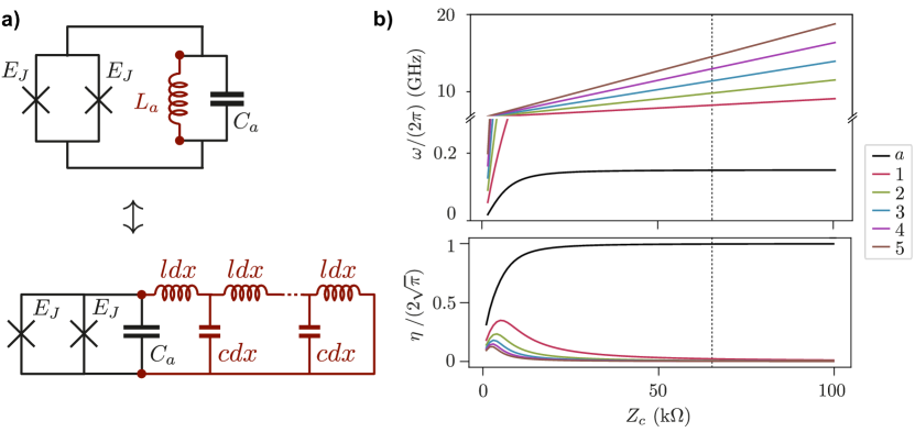
Figure S5: Array modes of the superinductor. a) A realistic superinductor is modeled by a transmission line with large inductance per unit length $l$ and stray capacitance to ground per unit length $c$ (in red). Such a realistic model for the target mode inductance $L_{a}$ (ancillary mode used for dissipation engineering not represented) leads to spurious resonances known as array modes. b) Frequency (top) and vacuum phase fluctuations across the Josephson ring (bottom) of the target mode (black) and the first five array modes (in color), all loaded by the target mode shunt capacitance $C_{a}$, as a function of the characteristic impedance $Z_{c}=\sqrt{l/c}$ of the inductor. Other circuit parameters are those of Tab. 1, and in particular, the total inductance $L_{a}=14~{}\mu\mathrm{H}$ is fixed. The dashed line represents the highest reported value of $Z_{c}$ in the literature [42].

The superconducting gap of aluminium places a hard limit around 90 GHz on the maximum frequency at which Josephson junctions built from this material can be driven. In practice, most laboratory equipment and circuitQED architectures have a narrower working bandwidth of 20 GHz. Moreover, in our proposal, we have neglected the intrinsic capacitance of the Josephson junctions forming the circuit ring, which is equivalent to assuming that the circuit is only biased below each junction plasma frequency $\omega_{J}=\sqrt{8E_{J}E_{c_{J}}}/\hbar$, where $E_{J}$ is the Josephson energy of each junction and $E_{c_{J}}$ its charging energy. This plasma frequency typically lies in the 10—50 GHz range, with its exact value depending on the thickness of the oxide barrier of the junction. In Tab. 1, we choose to limit the frequency comb bandwidth to 0—20 GHz and set the target resonator to 150 MHz in order to fit a hundred harmonics of the target mode frequency in this limited bandwidth (assuming the comb to be centered at 5 GHz, which is the ancillary mode frequency). Even though less conservative hypotheses may be considered for the junctions plasma frequency and bandwidth of the control electronics, the hard limit mentioned above prompts the need for such low frequency target mode. Since the mode impedance is set to $Z_{a}=2R_{Q}$, an inductance $L_{a}$ in the tens of $\mu$H range needs to be employed (see Tab. 1).

Currently, the most promising technologies for such superinductors are chains of Josephson junctions [66], disordered superconducting films [95] and planar superconducting coils [96]. These metallic structures typically have a $\sim$mm size and suffer from stray capacitance to ground. In Fig. 6a, we model such a realistic superinductor as a continuous transmission line of length $\lambda$, inductance per unit length $l$ (with $L_{a}=l\lambda$) and capacitance per unit length $c$ (for the sake of simplicity, the ancillary mode involved in dissipation engineering is not represented). This circuit hosts spurious resonances known as array modes of the superinductor [97], which have two advert effects. First, by diluting the target mode inductive energy over multiple inductors, which are not directly connected to the ring, they tend to decrease its vacuum phase fluctuations $\eta_{a}$ across the Josephson ring. Second, array modes (labeled by an integer $k\geq 1$) will appear in the circuit Hamiltonian (12) as spurious ancillary modes, the generalized phase operator across the ring becoming

$${\bf\Phi}=\varphi_{0}\big{(}\eta_{a}{\bf q}_{a}^{0}+\eta_{b}{\bf q}_{b}^{0}+\sum_{k}\eta_{k}{\bf q}_{k}^{0}\big{)},$$ (S182)

where ${\bf q}_{\cdot}^{0}$ designates a quadrature operator in the laboratory frame as in (12) and $\eta_{\cdot}$ represents the phase fluctuations of a mode across the ring. Even though we have not quantitatively investigated the impact of such modes on the GKP qubit lifetime, their proliferation with non-negligible phase fluctuations across the ring (i.e. $\eta_{k}\gtrsim\eta_{b}$) will lead to frequency collisions and inadvertent activation of high-order multimode processes, invalidating the two-mode picture presented in Sec. V.2 and Sec. S3.

Since the total inductance $L_{a}=\lambda l$ is fixed (see Tab. 1), the superinductor is fully characterized by its characteristic impedance $Z_{c}=\sqrt{l/c}$. This figure of merit sets both the frequency $\omega_{k}$ of array modes and their vacuum phase fluctuations across the ring $\eta_{k}$. In Fig. S5b, we represent these values for the first five array modes, extracted with the method of energy participation ratios [98] in the spirit of [60], as a function of $Z_{c}$. All other circuit parameters are those proposed in Tab. 1. We find that the array modes frequency increases and their fluctuations across the ring decreases with $Z_{c}$, with phase fluctuations becoming negligible for $Z_{c}\gg Z_{a}=13~{}\mathrm{k}\Omega$. Quantitatively, for the characteristic impedance of $65~{}\mathrm{k}\Omega$ recently reported for a Josephson junction chain released from its substrate [42] (dashed line in Fig. S5b), we find that fewer than 10 array modes lie in the frequency comb bandwidth, each with phase fluctuations $\eta_{k}\ll\eta_{b}$, justifying their omission in our model.

An important remark is in order here. In the inductor model of Fig. 6a, we have assumed the device inductance to be purely linear. For an implementation based on a chain of Josephson junctions, this model is only accurate if two conditions are met (we refer the reader to Refs. [99, 100] for a detailed analysis). First, the number $N_{J}$ of junctions in the chain should be sufficiently large and the individual inductance of the junctions sufficiently small—remember that $N_{J}\frac{\varphi_{0}^{2}}{E_{J}}=L_{a}$—that phase-slips through the array occur at a negligible rate (requiring $E_{J}\gg E_{c_{J}}$) and that the Kerr non-linearity induced on the target mode is negligible (scaling in $1/N_{J}^{2}$). Second, we have neglected the intrinsic shunt capacitance of each junction. When included in the circuit model, these capacitances curve the dispersion relation of array modes, whose frequency saturates at the plasma frequency $\omega_{p}$. Our model is thus only correct if $\omega_{p}$ is much larger than the frequency comb bandwidth. Superinductors based on nanometric scale tracks of granular aluminium, which effectively behave as long chains of large junctions with high plasma frequency ($\omega_{J}\sim 70~{}$GHz in Ref. [100]) appear to meet these requirements. We consider that the record characteristic impedance mentioned above (dashed line in Fig. S5b) will probably be surpassed in this type of architecture in the near future [101].

S4.2 Excessive target mode impedance

We remind the reader that the target mode impedance $Z_{a}=2R_{Q}$ was chosen so that, in reduced phase-space coordinates $(q,p)$, the target mode vacuum phase fluctuations across the Josephson ring $\eta_{a}=\sqrt{2\pi Z_{a}/R_{Q}}$ match the square GKP code lattice unit cell length. The GKP lattice can however be continuously distorted as long as the unit cell area in phase-space remains $4\pi$. Explicitly, the modular operators $e^{i\tilde{\eta}{\bf q}}$ and $e^{i\tilde{\eta}{\bf s}}$, where $\tilde{\eta}>\eta$, ${\bf s}={\bf R}_{\theta}{\bf q}{\bf R}^{\dagger}_{\theta}$ and $\mathrm{Sin}(\theta)=(\eta/\tilde{\eta})^{2}$, are the stabilizers of a diamond shaped lattice GKP. As pictured in Fig. S6, when the impedance of the target mode exceeds $2R_{Q}$, one simply adapts the timing of the bias pulses to stabilize such a non-square GKP code. Fig. S6 represents such a situation in the case of Hamiltonian engineering as described in Sec. IV, but is directly adaptable when engineering modular dissipation. Note that in the latter case, the normalizing envelope of the stabilized grid states envelope remains a rotational-symmetric Gaussian.

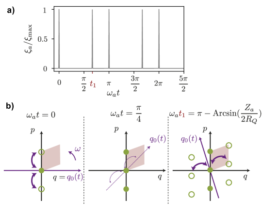
Figure S6: Adapting the GKP lattice to the target mode impedance a) When the target mode impedance $Z_{a}$ exceeds $2R_{Q}$, the timing of the bias pulses needs to be adapted so that b) in the target mode phase-space with axes $(q,p)$ rotating at $\omega_{a}$, Josephson tunneling triggers coherent displacements by $\pm\sqrt{2\pi Z_{a}/R_{Q}}$ along a diamond-shaped lattice with unit cell area $4\pi$ (in pink). The method is presented here for the case of Hamiltonian engineering.

Crucially, the angle $\theta$ only needs to be adjusted within some realistic margin of tolerance to avoid spurious logical errors. This tolerance depends on the dissipation parameter $\epsilon$. Intuitively, $\epsilon$ sets the extension of code states in phase-space. Errors appear when this extension is sufficient to sense the oscillating pseudo-potential from the modular dissipation going out of phase with the GKP lattice. In order to quantitatively estimate the required precision, we perturb the Lindblad operators entering the Lindblad dynamics of a stabilized GKP qubit by choosing a value $\eta_{a}$ slightly deviating from its ideal value $\eta_{0}=2\sqrt{\pi}$; this deviation models the residual uncertainty on the value of $\eta_{a}$ after adjustment of the chosen unit cell. We then numerically compute the logical decay rate $\Gamma_{L}$ of the generalized Pauli operators ${\bf X}$ and ${\bf Z}$. On Fig. S7, we present the dependence of this decay rate on the ratio $\eta_{a}/\eta_{0}$. We find that the value of $\eta_{a}$ (or equivalently $\theta$ when actively compensating for a known bias) needs to be adjusted at the $10^{-2}$ to $10^{-3}$ level to preserve the performance of the stabilization scheme; as expected, the smaller values of $\epsilon$ lead to the most stringent requirements on $\theta$.

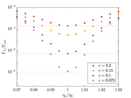
Figure S7: Logical error rate as a function of the relative error $\eta_{a}/\eta_{0}$ on the value of $\eta_{a}$ with respect to its ideal value $\eta_{0}=2\sqrt{\pi}$. Colored dots correspond to numerically extracted decay rates, while dotted lines indicate the theoretical asymptotic value of the decay rates only stemming from the finite energy of the stabilized GKP code.

S4.3 Josephson junctions asymmetry

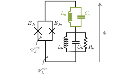
Figure S8: Compensating for Josephson junctions asymmetry We recall the circuit proposed to engineer modular dissipation in Fig. 6a A Josephson ring is placed in parallel of a high-impedance target resonator (green) and a low-impedance, dissipative, ancillary resonator (black). The Josephson tunneling amplitude $2E_{J}\xi(t)$ and phase are adjusted with the control fluxes $\Phi_{J,L}^{\mathrm{ext}}$ biasing the circuit. Here, we consider the possibility that the ring junctions have slightly different energies $E_{J_{1}}$ and $E_{J_{2}}$.

The energy of Josephson junctions is never perfectly reproducible, with a typical mismatch of the order of a percent between two nominally identical junctions in the same device. When the two junctions forming the ring of the circuit depicted in Fig. S8 have slightly different energies $E_{J_{1}}$ and $E_{J_{2}}$, the amplitude of Josephson tunneling cannot be perfectly cancelled by threading the ring with half a flux quantum ($\Phi^{\mathrm{ext}}_{J}=\varphi_{0}\pi$), as proposed in Sec. V.2. We remind the reader that in our protocol, tunneling is only triggered by fast flux pulses when the Josephson phase operator $\Phi$ aligns with the GKP lattice axes in the target oscillator rotating frame: imperfect cancellation of Josephson tunneling in between pulses may lead to long shifts of the oscillator state along a random axis and cause logical errors.

We propose to mitigate this advert effect by adjusting the circuit DC flux bias so that the spurious Josephson tunneling term becomes non-resonant and drops out in the RWA. Letting $E_{\Sigma}=E_{J_{1}}+E_{J_{2}}$ and $E_{\Delta}=E_{J_{1}}-E_{J_{2}}$, we thus set

$$\begin{split}\Phi^{\mathrm{ext}}_{J}=&\varphi_{0}(\pi-2A-2B)\\ \Phi^{\mathrm{ext}}_{L}=&-\frac{\Phi^{\mathrm{ext}}_{J}}{2}+\varphi_{0}\frac{\pi}{4}\end{split}$$ (S183)

where $B=\mathrm{Arcsin}(\xi)$ is the same AC bias signal as described in Sec. V.2 and $A=\mathrm{Arctan}(d)$ is a small DC offset that depends on the junctions asymmetry $d=\frac{E_{\Delta}}{E_{\Sigma}}$. Denoting $\bm{\varphi}={\bf\Phi}/\varphi_{0}=\eta_{a}{\bf q}_{a}+\eta_{b}{\bf q}_{b}$ the reduced phase across the ring, the ring contribution to the circuit Hamiltonian reads

$$\begin{split}{\bf H}_{J}&=-E_{J_{1}}\mathrm{cos}\left(\frac{{\bf\Phi}-\Phi^{\mathrm{ext}}_{J}-\Phi^{\mathrm{ext}}_{L}}{\varphi_{0}}\right)-E_{J_{2}}\mathrm{cos}\left(\frac{{\bf\Phi}-\Phi^{\mathrm{ext}}_{L}}{\varphi_{0}}\right)\\ &=-E_{J_{1}}\mathrm{cos}(\bm{\varphi}-\frac{3\pi}{4}+A+B)-E_{J_{2}}\mathrm{cos}(\bm{\varphi}+\frac{\pi}{4}-A-B)\\ &=-E_{\Sigma}\mathrm{cos}(\bm{\varphi}-\frac{\pi}{4})\mathrm{sin}(A+B)-E_{\Delta}\mathrm{sin}(\bm{\varphi}-\frac{\pi}{4})\mathrm{cos}(A+B)\end{split}$$ (S184)

Expanding the cosine and sine terms and using that $E_{\Sigma}\mathrm{sin}(A)=E_{\Delta}\mathrm{cos}(A)$, we find that

$${\bf H}_{J}=-E_{\Sigma}\big{(}\frac{1+d^{4}}{1+d^{2}}\big{)}^{\frac{1}{2}}\xi\mathrm{cos}(\bm{\varphi}-\frac{\pi}{4}+e)-E_{\Sigma}\big{(}\frac{2d^{2}}{1+d^{2}}(1-\xi^{2})\big{)}^{\frac{1}{2}}\mathrm{sin}(\bm{\varphi})$$ (S185)

where $e=\mathrm{Arctan}(d^{2})$. We now remark that, since the $\mathrm{sin}(\bm{\varphi})$ operator in the rightmost term only contains operators of the form $({\bf a}+{\bf a^{\dagger}})^{k}({\bf b}+{\bf b^{\dagger}})^{l}$ with $k+l$ an odd number, while the time-varying prefactor $(1-\xi^{2})^{1/2}$ has non-zero Fourier coefficients only for $\omega=k^{\prime}\omega_{a}+l^{\prime}\omega_{b}$ with $k^{\prime}+l^{\prime}$ an even number, this spurious term does not contribute in the RWA. As for the leftmost term, it is similar to the Hamiltonian (13), but for a prefactor close to 1 and a phase offset close to 0 when the junction asymmetry is small. These corrections only slightly modify the dissipation rates of the four engineered dissipators, which can be compensated for by adjusting the relative amplitudes of the four bias signals. Note that the RWA is valid for $\sqrt{2}E_{\Delta}\ll\omega_{a}$. In Tab 1, we choose the value of $E_{J}$ so that $\sqrt{2}E_{\Delta}\simeq\omega_{a}/10$ for junctions with asymmetry $d=1\%$ (corresponding to an energy mismatch of $2\%$ as quoted in the main text).

S4.4 Miscalibration of the control signals

As explained in Section VI.1, two main limitations prevent us from using the theoretical control signals defined in Eq. 14, which are linear combination of periodic Dirac combs. The restriction to periodic control signals with finite bandwidth was already studied in Section S3. However, even for a finite bandwidth signal, one also has to take into account the uncertainty introduced by the unknown dispersion of the feedlines that carry the signals, generated at room temperature, to the superconducting circuit. In practice, this dispersion relation has to be determined experimentally in a preliminary calibration procedure. To quantify the relative precision required in this calibration step, we study the impact of imperfect calibration, modeled as random noise affecting the control signals. More precisely, we replace each desired periodic controls $\xi(t)$ by an imperfectly calibrated signal $\tilde{\xi}(t)$ in which the Fourier coefficients of the target signal are multiplied by independent random coefficients close to 1:

$$\xi_{k}\mapsto\tilde{\xi}_{k}=s_{k}\,\xi_{k}$$

with $s_{k}\sim 1+\frac{\sigma_{\textrm{control}}}{\sqrt{2}}\left(\mathcal{N}(0,1)+i\mathcal{N}(0,1)\right).$ The noise coefficients $s_{k}$ are complex-valued, independent Gaussian coefficients with mean $1$ and variance $\sigma_{\textrm{control}}^{2}$.

The miscalibrated control signal $\tilde{\xi}$ is still a periodic signal, which we can feed into the RWA analysis presented in Section S3 to determine the effective dynamics at first order. For a given realization of the random noise coefficients, we can thus compute the logical decoherence rate associated to the dynamics

$$\frac{d\bm{\rho}_{t}}{dt}=\Gamma\sum_{k=0}^{3}\mathcal{D}[\tilde{\bf L}_{k}]\bm{\rho}_{t}$$ (S186)

where the desired Lindblad operators ${\bf L}_{k}$ are replaced by the effective operators obtained through RWA with miscalibrated control signals.

On Fig. S9, we represent the dependence of the logical decoherence rate on the standard deviation $\sigma_{\textrm{control}}$ modeling the relative precision of the calibration. Contrary to many figures in the paper, we do not observe an exponential decay of the decoherence rate with $\sigma_{\textrm{control}}$. This indicates that a rather precise calibration of the dispersion of the feedlines is required; numerically, we estimate that a relative accuracy around $0.1\%$, which we still consider experimentally realistic, is sufficient to maintain the logical decoherence rate several orders of magnitude below the engineered dissipation rate.

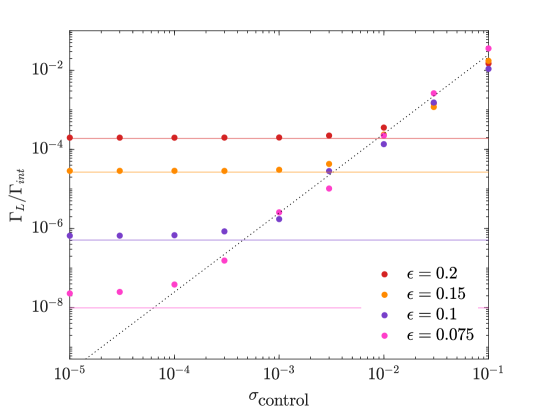
Figure S9: Dependence of the logical decoherence rate on the uncertainty on the complex amplitude of the harmonics of the control. The dots correspond to decoherence rates extracted from numerical simulations, where the full lines correspond to the asymptotic ideal rates obtained in Section S2.1. The black dotted line is proportional to $\sigma_{\textrm{control}}^{2}$ to serve as a guide for the eye. Beware that this figures uses a logarithmic scale, as opposed to a semi-logarithmic scale. The observed dependence is thus polynomial (approximately quadratic in $\sigma_{\textrm{control}}$, i.e. linear in the variance of the uncertainty) and not exponential. This figure presents the results obtained for one random realization of the noise coefficients, rather than an average over multiple realizations.

S5 Protected measurement of a Pauli operator

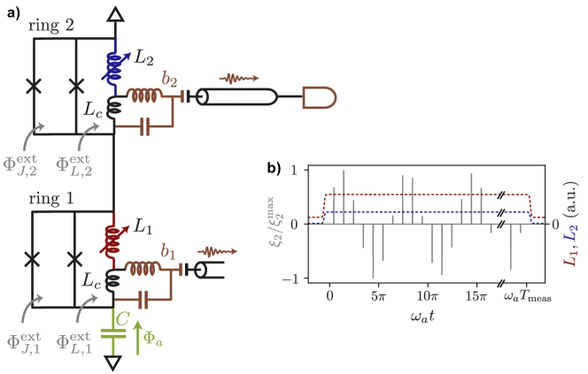
Figure S10: Protected readout of a GKP qubit a) The target mode (in green) participates in two Josephson rings with tunable inductors, allowing to independently adjust its phase fluctuations across each ring. Each ring is inductively connected to an ancillary mode (in brown, $L_{c}\ll L_{1},L_{2}$), dissipating photons into a transmission line (wriggled arrows). The ring 1 (constant phase fluctuations $\eta_{a,1}=2\sqrt{\pi}$) mediates an always-on modular dissipation stabilizing the code manifold, while the ring 2 (varied phase fluctuations $\eta_{a,2}$) can activate a longitudinal interaction between the logical qubit and the ancillary mode $b_{2}$ and is monitored with a high-efficiency homodyne detector (brown rounded rectangle). b) When measuring the logical qubit, $\eta_{a,2}$ is ramped up to $\sqrt{\pi}$ by adjusting the value of both inductances (red and blue dashed lines). A Dirac comb modulating a carrier at $\omega_{b_{2}}$ (signal $\xi_{2}$ in gray applied via the flux controls $\Phi^{\mathrm{ext}}_{J,2}$ and $\Phi^{\mathrm{ext}}_{L,2}$ of Eq. (S187)) activates the desired longitudinal interaction. After the measurement, $\eta_{a,2}$ is ramped down to $\eta^{\mathrm{idle}}_{a,2}\ll 1$ to suppress dephasing of the logical qubit by shot-noise in $b_{2}$.

In Sec. V.2 and Sec. S3, we showed how to engineer modular interactions between the target mode and a dissipative ancillary mode in order to stabilize the GKP code. In that scheme, the target mode effectively interacts with the ancilla via modular operators with spatial frequency set by its vacuum phase fluctuations $\eta_{a,1}$ across a parametrically modulated Josephson ring labeled 1. We choose $\eta_{a,1}=2\sqrt{\pi}$ so that these modular operators match the code stabilizers ${\bf S}_{q}=e^{i2\sqrt{\pi}{\bf q}_{a}}$ and ${\bf S}_{p}=e^{i2\sqrt{\pi}{\bf p}_{a}}$. Since the generalized Pauli operators ${\bf Z}=\mathrm{Sgn}\big{(}\mathrm{cos}(\sqrt{\pi}{\bf q})\big{)}$ and ${\bf X}=\mathrm{Sgn}\big{(}\mathrm{cos}(\sqrt{\pi}{\bf p})\big{)}$ have a twice smaller spatial frequency, accessing their value while maintaining the code stabilization requires the target mode to participate in a second Josephson ring, labeled 2, with twice smaller vacuum fluctuations $\eta_{a,2}=\sqrt{\pi}$. Fig. S10a pictures such a situation. Here, we represent an actual circuit and not a Foster synthesis of the environment seen by the junctions as in Fig. 6. Two Josephson rings, each weakly coupled to an ancillary mode (in brown $L_{c}\ll L_{1},L_{2}$), are placed in series of a capacitor, forming the target mode $a$. We neglect the capacitance of the junctions as it is not expected to play a role in the following as long as the circuit is driven safely below the junctions plasma frequency. The rings shunt inductances $L_{i}$ ($i=1,2$) are made tunable—for instance by implementing them with chains of Josephson rings controlled with an external magnetic field, not shown—so that the total shunt inductance $L=L_{1}+L_{2}$ and the rings participation ratio $p_{i}=\frac{L_{i}}{L}$ can be adjusted in situ. By adjusting the value of $L_{1}$ and $L_{2}$, we thus control independently the target mode vacuum fluctuations $\eta_{a,i}=p_{i}\sqrt{\frac{L}{C}}=2\sqrt{\pi}$ across each ring. In the following, $\eta_{a,1}$ is held constant at all time (during readout and outside readout time), and the ring is always threaded with the control biases $\Phi^{\mathrm{ext}}_{J,1}$ and $\Phi^{\mathrm{ext}}_{L,1}$ described in Sec. V.2 and Sec. S3 so that the modular dissipation is always active .

We consider the following controls for the ring 2

$$\begin{split}\Phi^{\mathrm{ext}}_{J,2}&=\varphi_{0}\big{(}\pi+2\mathrm{Arcsin}(\xi_{2}(t)\big{)}\\ \Phi^{\mathrm{ext}}_{L,2}&=-\frac{\Phi^{\mathrm{ext}}_{J,2}}{2}+\varphi_{0}\frac{\pi}{2}\end{split}$$ (S187)

such that the ring contributes, in the rotating frame of the modes $a$ and $b_{2}$, to the circuit Hamiltonian with

$${\bf H}_{2}(t)=2E_{J}\xi_{2}(t)~{}\mathrm{sin}\big{(}\eta_{a,2}{\bf q}^{0}_{a}(t)+\eta_{b_{2}}{\bf q}^{0}_{b_{2}}(t)\big{)}.$$ (S188)

Here as in (12), ${\bf q}^{0}_{a}$, ${\bf q}^{0}_{b_{2}}$ are laboratory frame quadrature operators respectively rotating at $\omega_{a}$ and $\omega_{b_{2}}$ in the rotating frame.

When measuring the logical qubit, say along ${\bf Z}$, we set $\eta_{a,2}=\sqrt{\pi}$ and apply a control signal made of a single Dirac comb modulating a carrier at $\omega_{b_{2}}$

$$\xi_{2}(t)=\xi_{\mathrm{int}}{}_{\frac{\pi}{\omega}}(t)\mathrm{cos}(\omega_{b_{2}}t)$$ (S189)

activating the ring 2 Josephson energy when the operator ${\bf q}^{0}_{a}$ aligns with the rotating frame quadrature operator ${\bf q}_{a}$. In this expression, $\xi_{\mathrm{int}}$ is the integrated amplitude of a single pulse of the comb. Following the method detailed in Sec. S3, we find that the effective interaction Hamiltonian in the RWA reads

$${\bf H}_{\mathrm{meas}}=\hbar g_{\mathrm{meas}}\mathrm{cos}(\sqrt{\pi}{\bf q}_{a}){\bf q}_{b_{2}}$$ (S190)

where $g_{\mathrm{meas}}=\omega_{a}E_{J}\eta_{b_{2}}\xi_{\mathrm{int}}/(\pi\hbar)$. When projected onto the code manifold, this Hamiltonian approximates the so-called longitudinal interaction $\hbar g_{\mathrm{meas}}{\bf Z}{\bf q}_{b_{2}}$ between the logical qubit and the ancillary mode. By letting the ancillary mode field leak into a transmission line (black cylinder in Fig. S10a, photon exit rate $\kappa_{b_{2}}$) fed to a high-efficiency homodyne detection chain (brown rounded rectangle), the logical qubit is continuously measured at a rate $\Gamma_{\mathrm{meas}}\simeq\frac{4g_{\mathrm{meas}}^{2}}{\kappa_{b_{2}}}$. ${\bf X}$ and ${\bf Y}$ measurements can be performed in a similar manner, albeit setting $\eta_{a,2}=\sqrt{2\pi}$ when measuring ${\bf Y}$. Note that the interaction Hamiltonian (S190) does not preserve the finite-energy code states so that the measurement rate should remain smaller than the confinement strength onto the code manifold $\Gamma_{\mathrm{meas}}\ll\Gamma_{c}=\epsilon 2\sqrt{\pi}\epsilon\Gamma$ with $\Gamma$ the modular dissipation rate. This criterion is required for the measurement to be Quantum Non Demolition (QND). The readout signal may then be integrated for a duration $T_{\mathrm{meas}}$ with $1/\Gamma_{\mathrm{meas}}\ll T_{\mathrm{meas}}\ll 1/\Gamma_{L}$ to yield a high fidelity readout, solely limited by the decay rate $\Gamma_{L}$ of the generalized Pauli operators. Combining this measurement with feedback Clifford gates (see Sec. VII), the logical qubit can be initialized at any cardinal point of the Bloch sphere.

Outside of measurement times, we set $\xi_{2}=0$. Crucially, we can make sure that no logical information unintentionally leaks out of the system even if $\xi_{2}$ fluctuates around its null value or if the ancillary mode ${\bf b}_{2}$ is subject to noise. To this end, when not measuring the logical qubit, we ramp down $L_{2}$ to limit the vacuum fluctuations of the target mode across the ring 2 to $\eta^{\mathrm{idle}}_{a,2}\ll 1$ while $L_{1}$ is simultaneously ramped up to keep constant fluctuations across the ring 1 (see Fig. S10b). In this regime, the ring 2 only mediates interaction with the target mode via low-weight operators, and induced errors are corrected by the modular dissipation.

S6 Details of numerical simulations

S6.1 Scope of the simulations.

In this paper, we do not try to simultaneously study all sources of errors, resulting from experimental limitations (finite bandwidth of the control signals, stroboscopic implementations of each dissipator, etc.) as well as imperfections of the device (loss channels, Hamiltonian perturbations, uncertainty on the parameters, etc.). For each type of error, we rather study its impact on logical performance under the assumption that everything else is perfect: for instance, controls with limited bandwidth, which yield imperfect stabilizing dissipators, are studied without taking into account loss channels such as photon loss, etc. whereas these channels, in turn, are studied with perfect dissipators. Our goal is to understand precisely the contribution of each type of possible errors in isolation. This allows us to roughly identify a parameter regime, that is a set of (possibly over-optimistic) constraints on all the experimental parameters entering the dynamics, under which each source of error, taken separately, leads to a reasonable degradation of the logical performance of a GKP qubit. In particular, it should be understood that our goal is not to precisely simulate a given experiment (which does not exist yet!), but to help in its future design, by identifying possible experimental challenges in implementing our proposal and quantifying the experimental developments that will be required to enter this favorable parameter regime (in terms of e.g. device imperfections, precision of calibrations, microwave control, etc.).

S6.2 Numerical scheme

Several solutions coexist to compute the solution of Lindblad master equations, that we can schematically sort into two categories:

1. Use already available general-purpose routines for the simulation of dynamical systems (such as Runge-Kutta methods, implicit Adams methods, etc.). This is the solution used in popular quantum libraries such as QuTiP [103, 104], QuantumOptics.jl [105] or the newly announced Qiskit Dynamics [106].

   On the one hand, this solution leverages already existing, tested and optimized high-order schemes. On the other hand, it ignores the structure of the problem, in particular that the solution $\bm{\rho}$ must be a density operator. Thus, numerical errors can generate negativities in the computed solution [107], notably when the true solution of the problem features zero or small eigenvalues. We argue that this is in fact a generic property of any simulation of a qubit embedded in a bosonic mode, as the density operator of the system lives in an infinite-dimensional Hilbert space, truncated numerically to a given (possibly high) dimension, but encodes a qubit living in $\mathbb{C}^{2}$.

2. Use structure-preserving numerical schemes designed for the simulation of density operators [108, 109, 110] [111, Appendix B]. To the best of our knowledge, these schemes are not readily available in common quantum libraries, but have already been used in the literature.

Preliminary versions of the simulations presented in this paper relied on the QuTiP library to compute the solution of Lindblad master equations in the Fock basis. However, this solution turned out to be impractical due to the high dimension needed to accurately simulate the evolution of GKP states in the Fock basis. In particular, the most demanding simulations required up to $N=5000$ Fock states to observe numerical convergence (notably, to capture logical error rates as low as $10^{-8}$ from the numerical simulations). Moreover, the Lindblad operators entering the dynamics, such as ${\bf L}_{0}=e^{-\epsilon\eta/2}e^{i\eta{\bf q}}({\bf 1}-\epsilon{\bf p})-{\bf 1}$, do not have a sparse representation in the Fock basis (this is in stark contrast to other bosonic encodings, for instance the cat qubit encoding, where several stabilization schemes where proposed using only low-order polynomials in ${\bf a},{\bf a}^{\dagger}$, the sparse representation of which allows for efficient simulations even in high dimensions).

Additionally, we found that QuTiP suffers from a design flaw: to compute the solution of a Lindblad equation of the form $\frac{d}{dt}\bm{\rho}=\mathcal{L}\bm{\rho}$ in dimension $N$, where $\bm{\rho}$ is an $N\times N$ matrix, it first rewrites it to the equivalent equation $\frac{d}{dt}\hat{\bm{\rho}}=\hat{\mathcal{L}}\hat{\bm{\rho}}$ in dimension $N^{2}$, where $\hat{\bm{\rho}}$ is the vectorized representation of $\bm{\rho}$ (column stacked in an $N^{2}$ vector) and $\hat{\mathcal{L}}$ is the Liouvillian of the problem. While formally equivalent, this method requires $O(N^{4})$ storage capacity and the evaluation of $\hat{\mathcal{L}}\hat{\bm{\rho}}$ has a time complexity of $O(N^{4})$ (matrix-vector product in dimension $N^{2}$), while the evaluation of $\mathcal{L}\bm{\rho}$ has a time-complexity of only $O(N^{3})$ (matrix-matrix product in dimension $N$) and requires an $O(N^{2})$ storage capacity. For $N=5000$ in a dense problem, this design choice prohibits the use of QuTiP routines.
We thus implemented the first-order structure-preserving scheme proposed in [111, Appendix B]. It can be seen as a fully-linear refinement over the $\mathcal{A}^{1}$ scheme proposed in [110]. Whilst this is only a first-order scheme, in practice, we found that it was fast enough to achieve numerical convergence in reasonable runtimes on a laptop for all simulations presented in the paper . Note that in principle, explicit structure-preserving schemes of arbitrary order can be developed following [110].

For the sake of pedagogy, let us explain how to derive this scheme in the case of a generic, time-independent Lindblad equation of the form

$$\frac{d}{dt}\bm{\rho}_{t}=-i\,[{\bf H},\bm{\rho}_{t}]+\sum_{j=1}^{J}\mathcal{D}[{\bf L}_{j}](\bm{\rho}_{t}).$$ (S191)

A naive approach for the simulation of Eq. S191 is to use Euler’s explicit scheme of order $1$:

$$\bm{\rho}_{n+1}=\bm{\rho}_{n}+dt\left(-i\,[{\bf H},\bm{\rho}_{t}]+\sum_{j=1}^{J}\mathcal{D}[{\bf L}_{j}](\bm{\rho}_{t})\right)$$ (S192)

where $\bm{\rho}_{n}\simeq\bm{\rho}(ndt)$. This scheme is not structure-preserving. However, we can approximate it with a quantum channel up to second-order terms:

$$\bm{\rho}_{n+1} =\sum_{j=0}^{J}{\bf M}_{j}\,\bm{\rho}_{n}\,{\bf M}_{j}^{\dagger}=\bm{\rho}_{n}\ +dt\left(-i\,[{\bf H},\bm{\rho}_{t}]+\sum_{j=1}^{J}\mathcal{D}[{\bf L}_{j}](\bm{\rho}_{t})\right)+O(dt^{2})$$ (S193)

$${\bf M}_{0} ={\bf 1}+dt\left(-i{\bf H}-\frac{1}{2}\sum_{j=1}^{J}{\bf L}_{j}^{\dagger}{\bf L}_{j}\right)$$

$${\bf M}_{j} =\sqrt{dt}{\bf L}_{j},\quad 1\leq j\leq J.$$

This does not describe an exact quantum channel as $\sum_{j=0}^{J}{\bf M}_{j}^{\dagger}{\bf M}_{j}=1+O(dt^{2})$. The (non-linear) structure-preserving scheme $\mathcal{A}^{1}$ in [110] compensates this by explicitly enforcing the conservation of the trace:

$$\bm{\rho}_{n+1}=\mathcal{A}^{1}(\bm{\rho}_{n})=\frac{1}{\operatorname{Tr}\left(\left(\sum_{j=0}^{J}{\bf M}_{j}^{\dagger}{\bf M}_{j}\right)\bm{\rho}_{n}\right)}\,\sum_{j=0}^{J}{\bf M}_{j}\,\bm{\rho}_{n}\,{\bf M}_{j}^{\dagger}.$$ (S194)

We use instead the fully-linear version proposed in [111, Appendix B]:

$$\bm{\rho}_{n+1} =\sum_{j=0}^{J}{\bf N}_{j}\,\bm{\rho}_{n}\,{\bf N}_{j}^{\dagger}$$ (S195)

$${\bf N}_{j} ={\bf M}_{j}\left(\sum_{j=0}^{J}{\bf M}_{j}^{\dagger}{\bf M}_{j}\right)^{-1/2}.$$

Note that $\sum_{j=0}^{J}{\bf N}_{j}^{\dagger}{\bf N}_{j}={\bf 1}$ and ${\bf N}_{j}={\bf M}_{j}+O(dt^{2})$, which ensures the consistency of the scheme. Additionally, this normalization step needs to be performed only once (when the operators ${\bf H}$ and ${\bf L}_{j}$ are time-independent) so that its cost is negligible. We highlight that this is a general procedure, that could be applied to any numerical scheme expressed as a pseudo quantum channel, that is of the form $\bm{\rho}_{n+1}=\sum_{j}M_{j}\bm{\rho}M_{j}^{\dagger}$ where $\sum_{j}M_{j}^{\dagger}M_{j}\neq{\bf 1}$. The first-order scheme considered here could thus be replaced by any of the higher-order, positivity-preserving scheme proposed in [110], modified according to Eq. S195 to get a fully-linear scheme of the same order. In our experiments, we find that this linear, first-order scheme converges faster with $dt\rightarrow 0$ than the non-linear $\mathcal{A}^{1}$ scheme (both are first-order schemes but with different prefactors).

In practice, for the numerical simulation of Lindblad equation in the Fock basis, we have to choose a dimension truncation $N$ and a time-step $dt$. The time-step $dt$ is chosen to ensure numerical convergence of the scheme on a given simulation (i.e. $dt$ is decreased until the results reach a stationary value). On the other hand, for the simulation of a GKP dynamics, the precise estimates of Section S2.2 indicate that the truncation should satisfy $N\gg\eta/\epsilon$. We additionally use the fact that we can explicitly compute logical errors rates induced by quadrature noise only (see Section S2.1) to determine the exact truncation : $N$ is increased until the simulated errors rates match those predicted by this exact analysis. We then use the same truncation in our other simulations where exact errors rates are not available due to the presence of other decoherence channels. We find that relatively high truncation are needed to accurately compute the exponentially small logical error rates presented in our figures; our simulations used truncations up to $N=5000$.

S6.3 Exact computations of the Lindblad operators in the Fock basis

We can compute explicitly (without any numerical approximation) the matrix elements in the Fock basis of any operator in the form

$${\bf L}_{\theta}=e^{i\theta{\bf N}}\left(e^{i\eta{\bf q}}\left({\bf 1}-\epsilon{\bf p}\right)-{\bf 1}\right)e^{-i\theta{\bf N}}$$

where $\theta\in\mathbb{R}$, $\eta>0$, $\epsilon>0$ (rather than, for instance, computing $e^{i\eta{\bf q}}$ by expressing ${\bf q}$ in a given truncation of the Fock basis, then computing its numerical matrix exponential, accumulating truncation errors along the way). This canvas encompasses all Lindblad operators proposed in our schemes for the stabilization of both square and hexagonal GKP codes; additionally, it is also sufficient for the computation of their approximate version obtained through modular dissipation engineering with control signals of limited bandwidth (see Section S3). The operators ${\bf p}=\frac{{\bf a}-{\bf a}^{\dagger}}{\sqrt{2}i}$ and ${\bf R}_{\theta}=e^{i\theta{\bf N}}$ have simple expression in the Fock basis:

$$\bra{m}{\bf p}\ket{n} =-\frac{i}{\sqrt{2}}\left(\sqrt{n}\,\delta_{m+1,n}-\sqrt{m}\,\delta_{m,n+1}\right),$$ (S196)

$$\bra{m}{\bf R}_{\theta}\ket{n} =e^{i\theta n}\,\delta_{m,n}.$$

On the other hand, the matrix elements of $e^{i\eta{\bf q}}$ are obtained through recurrence relations. The initialization is obtained by identifying $e^{i\eta{\bf q}}$ to a displacement operator as $e^{i\eta{\bf q}}={\bf D}(\frac{i\eta}{\sqrt{2}})$, so that:

$$\bra{0}e^{i\eta{\bf q}}\ket{n}=\bra{n}e^{i\eta{\bf q}}\ket{0} =\bra{n}{\bf D}\left(\tfrac{i\eta}{\sqrt{2}}\right)\ket{0}=\braket{n}{~(\tfrac{i\eta}{\sqrt{2}})_{c}}=e^{-\tfrac{\eta^{2}}{4}}\left(\frac{i\eta}{\sqrt{2}}\right)^{n}\frac{1}{\sqrt{n!}}$$ (S197)

where $\ket{(\tfrac{i\eta}{\sqrt{2}})_{c}}$ denotes the coherent states of amplitude $\frac{i\eta}{\sqrt{2}}$. The remaining matrix elements can then be computed through the following relations, where $\alpha=\frac{i\eta}{\sqrt{2}}$:

$$\bra{m+1}e^{i\eta{\bf q}}\ket{n+1} =\bra{m+1}{\bf D}(\alpha)\ket{n+1}$$ (S198)

$$=\frac{1}{\sqrt{(m+1)(n+1)}}\,\bra{m}{\bf a}\,{\bf D}(\alpha)\,{\bf a^{\dagger}}\ket{n}$$

$$=\frac{1}{\sqrt{(m+1)(n+1)}}\,\bra{m}{\bf a}({\bf a^{\dagger}}-\alpha^{*})\,{\bf D}(\alpha)\ket{n}$$

$$=\frac{1}{\sqrt{(m+1)(n+1)}}\,\Big{(}(m+1)\bra{m}{\bf D}(\alpha)\ket{n}-\alpha^{*}\bra{m}{\bf a}\,{\bf D}(\alpha)\ket{n}\Big{)}$$

$$=\frac{1}{\sqrt{(m+1)(n+1)}}\,\Big{(}(m+1)\bra{m}{\bf D}(\alpha)\ket{n}-\alpha^{*}\bra{m}{\bf D}(\alpha)\,({\bf a}+\alpha)\ket{n}\Big{)}$$

$$=\frac{1}{\sqrt{(m+1)(n+1)}}\,\Big{(}(m+1-|\alpha|^{2})\bra{m}{\bf D}(\alpha)\ket{n}-\alpha^{*}\bra{m}{\bf D}(\alpha)\,{\bf a}\ket{n}\Big{)}$$

$$=\frac{1}{\sqrt{(m+1)(n+1)}}\,\Big{(}(m+n+1-|\alpha|^{2})\bra{m}{\bf D}(\alpha)\ket{n}-\bra{m}{\bf D}(\alpha)\,({\bf a^{\dagger}}+\alpha^{*}){\bf a}\ket{n}\Big{)}$$

$$=\frac{1}{\sqrt{(m+1)(n+1)}}\,\Big{(}(m+n+1-|\alpha|^{2})\bra{m}{\bf D}(\alpha)\ket{n}-\bra{m}{\bf a^{\dagger}}\,{\bf D}(\alpha)\,{\bf a}\ket{n}\Big{)}$$

$$=\frac{1}{\sqrt{(m+1)(n+1)}}\,\Big{(}(m+n+1-|\alpha|^{2})\bra{m}{\bf D}(\alpha)\ket{n}-\sqrt{mn}\bra{m-1}{\bf D}(\alpha)\ket{n-1}\Big{)}$$

$$=\frac{m+n+1-\eta^{2}/2}{\sqrt{(m+1)(n+1)}}\,\bra{m}e^{i\eta{\bf q}}\ket{n}-\sqrt{\frac{mn}{(m+1)(n+1)}}\,\bra{m-1}e^{i\eta{\bf q}}\ket{n-1}$$

(where the last term appears only when $m,n>0$).

Since all coefficients of this recurrence relation are real, we can show that for any $n,m$,

$$\bra{m}e^{i\eta{\bf q}}\ket{n} =\bra{n}e^{i\eta{\bf q}}\ket{m},$$ (S199)

$$\bra{m}e^{i\eta{\bf q}}\ket{n} \in\mathbb{R}\quad\textrm{ if }m-n\textrm{ even},$$

$$\bra{m}e^{i\eta{\bf q}}\ket{n} \in i\mathbb{R}\quad\textrm{ if }m-n\textrm{ odd}.$$

We emphasize that using Eq. S198, each diagonal of the matrix of ${\bf L}_{\theta}$ in the Fock basis can be computed independently; in practice, when dealing with control signals of limited bandwidth, we need only compute as many diagonals as the number of harmonics in the control signal (see Section S3). Additionally, computing the hermitian (respectively anti-hermitian) part of ${\bf L}_{\theta}$ as in Section V amounts to computing separately the even (respectively odd) diagonals of ${\bf L}_{\theta}$.

Finally, using Eq. S199 we can reformulate the previous matrix decomposition along diagonals as the following operator decomposition:

$$e^{i\eta{\bf q}}=\phi_{0}({\bf N};\eta)+\sum_{k=1}^{+\infty}i^{k}\left(\phi_{k}({\bf N};\eta)\,{\bf a}^{k}+{\bf a}^{\dagger k}\,\phi_{k}({\bf N};\eta)\right)$$ (S200)

where the $\phi_{k}$ are real-valued functions defined by

$$\phi_{k}(n;\eta)=i^{k}\sqrt{\frac{n!}{(n+k)!}}\,\bra{n}e^{i\eta{\bf q}}\ket{n+k}.$$ (S201)

S6.4 Extraction of logical error rates

The logical coordinates associated to a given density operator $\bm{\rho}$ are defined as the expectation values of the three generalized Pauli ${\bf X},{\bf Y},{\bf Z}$ operators. In other words, the encoded logical qubit is defined as

$$\bm{\rho}_{L}=\frac{{\bf 1}+\operatorname{Tr}({\bf X}\bm{\rho})\sigma_{X}+\operatorname{Tr}({\bf Y}\bm{\rho})\sigma_{Y}+\operatorname{Tr}({\bf Z}\bm{\rho})\sigma_{Z}}{2}$$ (S202)

where $\sigma_{X},\sigma_{Y},\sigma_{Z}$ are the usual Pauli operators on $\mathbb{C}^{2}$.

In Section S2.1 we show that, for both stabilization schemes proposed here (corresponding to square and hexagonal GKP codes), in presence of quadrature noise only, the expectation value of periodic observables (such as ${\bf X},{\bf Y},{\bf Z}$) evolve according to two timescales: an initial fast transient regime with a typical timescale $\tau_{conv}\sim\frac{1}{\epsilon\eta\Gamma}$ (where $\Gamma>0$ is the engineered dissipation rate), that we can interpret as a fast convergence to a coding state, followed by a slow decay with an exponentially larger typical timescale $\tau_{log}\gg\tau_{conv}$, that we can interpret as decoherence of the encoded logical qubit. In presence of generic decoherence channels (such as e.g. photon loss, Kerr effect or dephasing) we thus extract the logical error rates by the following procedure:

1. prepare an initial density operator $\bm{\rho}_{0}$ with non-zero logical coordinates $\operatorname{Tr}({\bf X}\bm{\rho}_{0}),\operatorname{Tr}({\bf Y}\bm{\rho}_{0}),\operatorname{Tr}({\bf Z}\bm{\rho}_{0})$;

2. let $\bm{\rho}_{t}$ evolve from $\bm{\rho}_{0}$ following the Lindblad dynamics under study, during a simulation time $T_{simu}\gg\tau_{conv}$;

3. compute the evolution of the logical coordinates $\operatorname{Tr}({\bf X}\bm{\rho}_{t}),\operatorname{Tr}({\bf Y}\bm{\rho}_{t}),\operatorname{Tr}({\bf Z}\bm{\rho}_{t})$ along the trajectory;

4. fit the post-transient dynamics with an exponential function of time.

For the initialization of the procedure with a density operator yielding a non-zero expectation value of ${\bf X},{\bf Y},{\bf Z}$, a numerically cheap strategy is to exploit the fact that finite-energy square GKP states are approximate ground states of the so-called square GKP Hamiltonian

$${\bf H}_{GKP,\textrm{square}}=\frac{\epsilon^{2}}{2}\left({\bf q}^{2}+{\bf p}^{2}\right)-\left(\cos(\eta{\bf q})+\cos(\eta{\bf p})\right)$$

while finite-energy hexagonal GKP states are approximate ground states of the so-called hexagonal GKP Hamiltonian

$${\bf H}_{GKP,\textrm{hexagonal}}=\frac{\epsilon^{2}}{2}\left({\bf q}^{2}+{\bf p}^{2}\right)-\frac{2}{3}\left(\cos(\eta{\bf q})+\cos(\eta{\bf q}_{\pi/3})+\cos(\eta{\bf q}_{2\pi/3})\right)$$

where ${\bf q}_{\theta}=\cos(\theta){\bf q}+\sin(\theta){\bf p}$ (note that the value of $\eta$ depends on the geometry). These two Hamiltonians are easy to compute numerically in the Fock basis using the tools of the previous section, and we use the eigenvectors corresponding to the lowest-lying eigenvalues as initial states. This choice is all the more motivated by the stability analysis led in Section S2.3.3, where we established that, with our dissipative stabilization scheme, this GKP Hamiltonian governs the “no-jump” part of the Lindblad evolution.

On Fig. S11, we illustrate this procedure for the computation of the logical error rate of a square GKP qubit subjected to photon loss, as studied in the top-right panel of Fig. 4, corresponding to the Lindblad equation

$$\frac{d}{dt}\bm{\rho} =\Gamma\sum_{k=0}^{3}\mathcal{D}[{\bf L}_{k}](\bm{\rho})+\kappa_{1\textrm{ph}}\,\mathcal{D}[{\bf a}](\bm{\rho})$$ (S203)

$${\bf L}_{k} =\mathcal{A}\,e^{ik\tfrac{\pi}{2}{\bf N}}\,e^{i\eta{\bf q}}\,\left({\bf 1}-\epsilon{\bf p}\right)e^{-ik\tfrac{\pi}{2}{\bf N}}\,-{\bf 1}$$

$$\bm{\rho}_{0} =\ket{\psi_{0}}\bra{\psi_{0}}$$

where $\eta=2\sqrt{\pi}$, $\epsilon$ is the energy-regularization parameter, $\mathcal{A}=e^{-\epsilon\eta/2}$, $\ket{\psi_{0}}$ is the eigenvector of ${\bf H}_{GKP,\textrm{square}}$ corresponding to its lowest eigenvalue, $\Gamma>0$ is the engineered dissipation rate and $\kappa_{1\textrm{ph}}$ is the photon loss rate. In practice, we expect from the analysis led in Section S2.1, confirmed by numerical experiments, that the post-transient logical decay rates are exponentially small functions of $\kappa_{1\mathrm{ph}}/\Gamma$, so that we cannot run simulations long enough to observe the full decay to zero of the logical coordinates. However, since the typical timescale of the transient $\tau_{\mathrm{conv}}=1/\mathcal{A}\epsilon\eta\Gamma$ does not depend on $\kappa_{1\mathrm{ph}}/\Gamma$, we restrict ourselves to running simulations for a time $T_{\mathrm{sim}}\gg\tau_{\mathrm{conv}}$ and fit the post-transient dynamics to an exponential function of time.

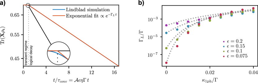
Figure S11: Extraction of logical error rates. a) Evolution on a logarithmic scale of the logical $x$-coordinate for a square GKP qubit subject to photon loss following Eq. S203. Here we fix $\epsilon=0.1$ and $\kappa_{1\textrm{ph}}/\Gamma=4\times 10^{-2}$. After a transient regime of typical timescale $\tau_{conv}=1/\mathcal{A}\epsilon\eta\Gamma$, we can fit the decay of the logical coordinate to an exponential proportional to $e^{-\Gamma_{L}\,t}$. Here, we find $\Gamma_{L}/\Gamma\simeq 9.7\times 10^{-3}$. b) We perform the previous procedure for varying values of $\epsilon$ and $\kappa_{1\textrm{ph}}$ to obtain the plot of $\Gamma_{L}/\Gamma$ as a function of $\kappa_{1\textrm{ph}}/\Gamma$, and plot the result against the corresponding theoretical value for quadrature noise for comparison. Note that this panel corresponds to Fig. 4b of the main text.

Note that the square GKP code has asymmetrical logical error rates associated to ${\bf X},{\bf Y},{\bf Z}$ satisfying

$$\Gamma_{L}^{X}=\Gamma_{L}^{Z}=\frac{1}{2}\Gamma_{L}^{Y}$$ (S204)

since a ${\bf Z}$ (respectively ${\bf X}$) error corresponds to a shift of length $\sqrt{\pi}$ along the $q$ (respectively $p$) axis in phase-space, while a ${\bf Y}$ error correspond to their composition, that is a longer shift of length $\sqrt{2\pi}$ along the diagonal. In the figures, the plotted logical error rates correspond to the value of $\Gamma_{L}^{X}$, from which we can immediately deduce the other two. For the hexagonal GKP code, on the other hand, these three values are identical thanks to the symmetry of the code.

S6.5 Simulations with finite-bandwidth control signals

Let us explain how one can analyze the impact of finite-bandwidth control signals, defined in Section S3, on the logical decoherence rate of our dissipative stabilization scheme.

Generally speaking, we see from the results of Section S3 that all considered control signals have the form

$$u(t)=g\sum_{r=-N}^{N}u_{r}e^{i(r\omega_{a}-\omega_{b})t},$$ (S205)

and we want to compute the effective Hamiltonian

$${\bf H}_{\mathrm{RWA}}^{(1)}=\overline{u(t)e^{i\eta_{a}{\bf q}_{a}(t)}e^{i\eta_{b}{\bf q}_{b}(t)}+\operatorname{h.c.}}$$ (S206)

from the Fourier coefficients $(u_{r})_{-N\leq r\leq N}$. Using the operator decomposition of Eq. S200, we get

$$e^{i\eta_{a}{\bf q}_{a}}e^{i\eta_{b}{\bf q}_{b}} =\left(\phi_{0}({\bf N}_{a};\eta_{a})+\sum_{{k_{a}}=1}^{+\infty}i^{k_{a}}\left(\phi_{k_{a}}({\bf N}_{a};\eta_{a})\,{\bf a}^{k_{a}}+{\bf a}^{\dagger{k_{a}}}\,\phi_{k_{a}}({\bf N}_{a};\eta_{a})\right)\right)$$ (S207)

$$\quad\quad\quad\quad\quad\left(\phi_{0}({\bf N}_{b};\eta_{b})+\sum_{{k_{b}}=1}^{+\infty}i^{k_{b}}\left(\phi_{k_{b}}({\bf N}_{b};\eta_{b})\,{\bf b}^{k_{b}}+{\bf b}^{\dagger{k_{b}}}\,\phi_{k_{b}}({\bf N}_{b};\eta_{b})\right)\right)$$

where ${\bf N}_{a}={\bf a}^{\dagger}{\bf a}$ and ${\bf N}_{b}={\bf b}^{\dagger}{\bf b}$; thus

$$u(t)e^{i\eta_{a}{\bf q}_{a}(t)}e^{i\eta_{b}{\bf q}_{b}(t)} =g\left(\sum_{r=-N}^{N}u_{r}e^{i(r\omega_{a}-\omega_{b})t}\right)$$ (S208)

$$\quad\quad\quad\quad\quad\left(\phi_{0}({\bf N}_{a};\eta_{a})+\sum_{{k_{a}}=1}^{+\infty}i^{k_{a}}\left(\phi_{k_{a}}({\bf N}_{a};\eta_{a})\,{\bf a}^{k_{a}}e^{-i{k_{a}}\omega_{a}t}+e^{i{k_{a}}\omega_{a}t}{\bf a}^{\dagger{k_{a}}}\,\phi_{k_{a}}({\bf N}_{a};\eta_{a})\right)\right)$$

$$\quad\quad\quad\quad\quad\left(\phi_{0}({\bf N}_{b};\eta_{b})+\sum_{{k_{b}}=1}^{+\infty}i^{k_{b}}\left(\phi_{k_{b}}({\bf N}_{b};\eta_{b})\,{\bf b}^{k_{b}}e^{-i{k_{b}}\omega_{b}t}+e^{i{k_{b}}\omega_{b}t}{\bf b}^{\dagger{k_{b}}}\,\phi_{k_{b}}({\bf N}_{b};\eta_{b})\right)\right).$$

Extracting the resonant terms from the previous expression, and assuming as always that $\omega_{a}$ and $\omega_{b}$ are incommensurate, we get

$$\overline{u(t)e^{i\eta_{a}{\bf q}_{a}(t)}e^{i\eta_{b}{\bf q}_{b}(t)}}$$ (S209)

$$\quad=ig\,\overline{\left(\sum_{r=-N}^{N}u_{r}e^{ir\omega_{a}t}\right)\left(\phi_{0}({\bf N}_{a};\eta_{a})+\sum_{{k_{a}}=1}^{+\infty}i^{k_{a}}\left(\phi_{k_{a}}({\bf N}_{a};\eta_{a})\,{\bf a}^{k_{a}}e^{-i{k_{a}}\omega_{a}t}+e^{i{k_{a}}\omega_{a}t}{\bf a}^{\dagger{k_{a}}}\,\phi_{k_{a}}({\bf N}_{a};\eta_{a})\right)\right)}{\bf b}^{\dagger}\,\phi_{1}({\bf N}_{b};\eta_{b})$$

$$\quad=ig\,\left(u_{0}\phi_{0}({\bf N}_{a};\eta_{a})+\sum_{{k_{a}}=1}^{N}i^{k_{a}}\left(u_{k_{a}}\phi_{k_{a}}({\bf N}_{a};\eta_{a})\,{\bf a}^{k_{a}}+u_{-k_{a}}{\bf a}^{\dagger{k_{a}}}\,\phi_{k_{a}}({\bf N}_{a};\eta_{a})\right)\right){\bf b}^{\dagger}\,\phi_{1}({\bf N}_{b};\eta_{b})$$

$$\quad=g{\bf A}_{u}\,{\bf B}^{\dagger}$$

where

$${\bf B} =-i\phi_{1}({\bf N}_{b};\eta_{b})\,{\bf b}$$ (S210)

$${\bf A}_{u} =u_{0}\phi_{0}({\bf N}_{a};\eta_{a})+\sum_{{k_{a}}=1}^{N}i^{k_{a}}\left(u_{k_{a}}\phi_{k_{a}}({\bf N}_{a};\eta_{a})\,{\bf a}^{k_{a}}+u_{-k_{a}}{\bf a}^{\dagger{k_{a}}}\,\phi_{k_{a}}({\bf N}_{a};\eta_{a})\right).$$

Note that, in the Fock basis, ${\bf A}_{u}$ can be computed by multiplying the diagonal, sub-diagonal and sur-diagonal of position at most $N$ of $e^{i\eta_{a}{\bf q}_{a}}$ by the corresponding Fourier coefficient of $u$; these diagonal decomposition can be computed efficiently as shown in Section S6.

All in all, we obtain

$${\bf H}_{\mathrm{RWA}}=g\left({\bf A}_{u}{\bf B}^{\dagger}+{\bf A}_{u}^{\dagger}{\bf B}\right)$$ (S211)

that we can compute for the four control signals $u_{0},\ldots,u_{3}$ corresponding to the four dissipators to engineer. Adding a resonant drive wherever required (to all Lindblad operators if we take the family $({\bf L}_{k})_{0\leq k\leq 3}$, or only to the symmetric Lindblad operators if we take the family of symmetric and antisymmetric Lindblad operators $({\bf L}_{r,l})_{r\in\{q,p\},\,l\in\{s,d\}}$), we get an effective Hamiltonian

$${\bf H} =g\left(({\bf A}_{u}-\sigma{\bf 1}){\bf B}^{\dagger}+({\bf A}_{u}-\sigma{\bf 1})^{\dagger}{\bf B}\right),\quad\sigma\in\{0,1\}$$ (S212)

$$=g\left({\bf L}_{u}{\bf B}^{\dagger}+{\bf L}_{u}^{\dagger}{\bf B}\right),$$

where $\sigma\in\mathbb{R}$ is the strength of the drive. We can directly feed this Hamiltonian into Eq. S116 in order to obtain an effective Lindblad equation after adiabatic elimination of mode $b$:

$$\frac{d\bm{\rho}_{t}}{dt}=\Gamma\,\mathcal{D}[{\bf L}_{u}](\bm{\rho}_{t})$$ (S213)

with $\Gamma=\frac{4g^{2}}{\kappa_{b}}|\phi_{1}(0;\eta_{b})|^{2}=\frac{4g^{2}}{\kappa_{b}}\frac{\eta_{b}^{2}}{2}\,e^{-\eta_{b}^{2}/2}$. We can then numerically simulate the dynamics

$$\frac{d\bm{\rho}_{t}}{dt}=\Gamma\,\sum_{k=0}^{3}\mathcal{D}[{\bf L}_{u,k}](\bm{\rho}_{t})$$ (S214)

to compute logical decoherence rates associated to the proposed finite-bandwidth control signals; the results are shown in Fig. 7 of the main text.

References

- Gottesman [1997] D. Gottesman, Stabilizer codes and quantum error correction (California Institute of Technology, 1997).
- Kitaev [2003] A. Y. Kitaev, Fault-tolerant quantum computation by anyons, Annals of Physics 303, 2 (2003).
- Freedman and Meyer [2001] M. H. Freedman and D. A. Meyer, Projective plane and planar quantum codes, Foundations of Computational Mathematics 1, 325 (2001).
- Bravyi and Kitaev [1998] S. B. Bravyi and A. Y. Kitaev, Quantum codes on a lattice with boundary, arXiv preprint quant-ph/9811052 (1998).
- Bombin and Martin-Delgado [2006] H. Bombin and M. A. Martin-Delgado, Topological quantum distillation, Physical review letters 97, 180501 (2006).
- Gottesman et al. [2001] D. Gottesman, A. Kitaev, and J. Preskill, Encoding a qubit in an oscillator, Phys. Rev. A 64, 012310 (2001).
- Grimsmo and Puri [2021] A. L. Grimsmo and S. Puri, Quantum error correction with the Gottesman-Kitaev-Preskill code, PRX Quantum 2, 020101 (2021).
- Cochrane et al. [1999] P. T. Cochrane, G. J. Milburn, and W. J. Munro, Macroscopically distinct quantum-superposition states as a bosonic code for amplitude damping, Phys. Rev. A 59, 2631 (1999).
- Mirrahimi et al. [2014] M. Mirrahimi, Z. Leghtas, V. V. Albert, S. Touzard, R. J. Schoelkopf, L. Jiang, and M. H. Devoret, Dynamically protected cat-qubits: a new paradigm for universal quantum computation, New J. Phys. 16, 045014 (2014).
- Michael et al. [2016] M. H. Michael, M. Silveri, R. Brierley, V. V. Albert, J. Salmilehto, L. Jiang, and S. M. Girvin, New class of quantum error-correcting codes for a bosonic mode, Phys. Rev. X 6, 031006 (2016).
- Hu et al. [2019] L. Hu, Y. Ma, W. Cai, X. Mu, Y. Xu, W. Wang, Y. Wu, H. Wang, Y. Song, C.-L. Zou, et al., Quantum error correction and universal gate set operation on a binomial bosonic logical qubit, Nat. Phys. 15, 503 (2019).
- Note [1] Mathematically, the oscillator operator appearing in the coupling Hamiltonian is a finite-order polynomial in and .
- Leghtas et al. [2015] Z. Leghtas, S. Touzard, I. M. Pop, A. Kou, B. Vlastakis, A. Petrenko, K. M. Sliwa, A. Narla, S. Shankar, M. J. Hatridge, et al., Confining the state of light to a quantum manifold by engineered two-photon loss, Science 347, 853 (2015).
- Flühmann et al. [2019] C. Flühmann, T. L. Nguyen, M. Marinelli, V. Negnevitsky, K. Mehta, and J. Home, Encoding a qubit in a trapped-ion mechanical oscillator, Nature 566, 513 (2019).
- Puri et al. [2018] S. Puri, A. Grimm, P. Campagne-Ibarcq, A. Eickbusch, K. Noh, G. Roberts, L. Jiang, M. Mirrahimi, M. H. Devoret, and S. M. Girvin, Stabilized cat in driven nonlinear cavity: A fault-tolerant error syndrome detector, arXiv preprint arXiv:1807.09334 (2018).
- Ma et al. [2020] W.-L. Ma, M. Zhang, Y. Wong, K. Noh, S. Rosenblum, P. Reinhold, R. J. Schoelkopf, and L. Jiang, Path-independent quantum gates with noisy ancilla, Physical Review Letters 125, 110503 (2020).
- Shi et al. [2019] Y. Shi, C. Chamberland, and A. Cross, Fault-tolerant preparation of approximate GKP states, New Journal of Physics 21, 093007 (2019).
- Siegele and Campagne-Ibarcq [2023] C. Siegele and P. Campagne-Ibarcq, Robust suppression of noise propagation in GKP error-correction, arXiv preprint arXiv:2302.12088 (2023).
- Rosenblum et al. [2018] S. Rosenblum, P. Reinhold, M. Mirrahimi, L. Jiang, L. Frunzio, and R. J. Schoelkopf, Fault-tolerant detection of a quantum error, Science 361, 266 (2018).
- Von Neumann [1996] J. Von Neumann, Mathematical Foundations of Quantum Mechanics (Princeton Univ. Press, Princeton, 1996).
- Aharonov et al. [1969] Y. Aharonov, H. Pendleton, and A. Petersen, Modular variables in quantum theory, Int. J. Theor. Phys. 2, 213 (1969).
- Popescu [2010] S. Popescu, Dynamical quantum non-locality, Nat. Phys. 6, 151 (2010).
- Flühmann et al. [2018] C. Flühmann, V. Negnevitsky, M. Marinelli, and J. P. Home, Sequential modular position and momentum measurements of a trapped ion mechanical oscillator, Phys. Rev. X 8, 021001 (2018).
- Travaglione and Milburn [2002] B. Travaglione and G. J. Milburn, Preparing encoded states in an oscillator, Phys. Rev. A 66, 052322 (2002).
- Pirandola et al. [2006] S. Pirandola, S. Mancini, D. Vitali, and P. Tombesi, Continuous variable encoding by ponderomotive interaction, Eur. Phys. J. D 37, 283 (2006).
- Terhal and Weigand [2016] B. Terhal and D. Weigand, Encoding a qubit into a cavity mode in circuit qed using phase estimation, Phys. Rev. A 93, 012315 (2016).
- Motes et al. [2017] K. R. Motes, B. Q. Baragiola, A. Gilchrist, and N. C. Menicucci, Encoding qubits into oscillators with atomic ensembles and squeezed light, Phys. Rev. A 95, 053819 (2017).
- Weigand and Terhal [2020] D. J. Weigand and B. M. Terhal, Realizing modular quadrature measurements via a tunable photon-pressure coupling in circuit QED, Physical Review A 101, 053840 (2020).
- Royer et al. [2020] B. Royer, S. Singh, and S. Girvin, Stabilization of finite-energy Gottesman-Kitaev-Preskill states, Physical Review Letters 125, 260509 (2020).
- Campagne-Ibarcq et al. [2020] P. Campagne-Ibarcq, A. Eickbusch, S. Touzard, E. Zalys-Geller, N. E. Frattini, V. V. Sivak, P. Reinhold, S. Puri, S. Shankar, R. J. Schoelkopf, et al., Quantum error correction of a qubit encoded in grid states of an oscillator, Nature 584, 368 (2020).
- de Neeve et al. [2022] B. de Neeve, T.-L. Nguyen, T. Behrle, and J. P. Home, Error correction of a logical grid state qubit by dissipative pumping, Nature Physics 18, 296 (2022).
- Kitaev [1995] A. Y. Kitaev, Quantum measurements and the abelian stabilizer problem, arXiv preprint quant-ph/9511026 (1995).
- Svore et al. [2013] K. M. Svore, M. B. Hastings, and M. Freedman, Faster phase estimation, arXiv preprint arXiv:1304.0741 (2013).
- Blais et al. [2021] A. Blais, A. L. Grimsmo, S. Girvin, and A. Wallraff, Circuit quantum electrodynamics, Reviews of Modern Physics 93, 025005 (2021).
- Cohen et al. [2017] J. Cohen, W. C. Smith, M. H. Devoret, and M. Mirrahimi, Degeneracy-preserving quantum nondemolition measurement of parity-type observables for cat qubits, Physical review letters 119, 060503 (2017).
- Mooij and Nazarov [2006] J. Mooij and Y. V. Nazarov, Superconducting nanowires as quantum phase-slip junctions, Nature Physics 2, 169 (2006).
- Astafiev et al. [2012] O. Astafiev, L. Ioffe, S. Kafanov, Y. A. Pashkin, K. Y. Arutyunov, D. Shahar, O. Cohen, and J. S. Tsai, Coherent quantum phase slip, Nature 484, 355 (2012).
- Le et al. [2019] D. T. Le, A. Grimsmo, C. Müller, and T. Stace, Doubly nonlinear superconducting qubit, Physical Review A 100, 062321 (2019).
- Brooks et al. [2013] P. Brooks, A. Kitaev, and J. Preskill, Protected gates for superconducting qubits, Physical Review A 87, 052306 (2013).
- Groszkowski et al. [2018] P. Groszkowski, A. Di Paolo, A. Grimsmo, A. Blais, D. Schuster, A. Houck, and J. Koch, Coherence properties of the 0- qubit, New Journal of Physics 20, 043053 (2018).
- Manucharyan et al. [2009] V. E. Manucharyan, J. Koch, L. I. Glazman, and M. H. Devoret, Fluxonium: Single Cooper-pair circuit free of charge offsets, Science 326, 113 (2009).
- Pechenezhskiy et al. [2020] I. V. Pechenezhskiy, R. A. Mencia, L. B. Nguyen, Y.-H. Lin, and V. E. Manucharyan, The superconducting quasicharge qubit, Nature 585, 368 (2020).
- Koch et al. [2007] J. Koch, M. Y. Terri, J. Gambetta, A. A. Houck, D. I. Schuster, J. Majer, A. Blais, M. H. Devoret, S. M. Girvin, and R. J. Schoelkopf, Charge-insensitive qubit design derived from the Cooper pair box, Physical Review A 76, 042319 (2007).
- Conrad et al. [2022] J. Conrad, J. Eisert, and F. Arzani, Gottesman-Kitaev-Preskill codes: A lattice perspective, Quantum 6, 648 (2022).
- Rymarz et al. [2021a] M. Rymarz, S. Bosco, A. Ciani, and D. P. DiVincenzo, Hardware-encoding grid states in a nonreciprocal superconducting circuit, Physical Review X 11, 011032 (2021a).
- Chapman et al. [2017] B. J. Chapman, E. I. Rosenthal, J. Kerckhoff, B. A. Moores, L. R. Vale, J. Mates, G. C. Hilton, K. Lalumiere, A. Blais, and K. Lehnert, Widely tunable on-chip microwave circulator for superconducting quantum circuits, Physical Review X 7, 041043 (2017).
- Lecocq et al. [2017] F. Lecocq, L. Ranzani, G. Peterson, K. Cicak, R. Simmonds, J. Teufel, and J. Aumentado, Nonreciprocal microwave signal processing with a field-programmable Josephson amplifier, Physical Review Applied 7, 024028 (2017).
- Barzanjeh et al. [2017] S. Barzanjeh, M. Wulf, M. Peruzzo, M. Kalaee, P. Dieterle, O. Painter, and J. M. Fink, Mechanical on-chip microwave circulator, Nature communications 8, 1 (2017).
- Mahoney et al. [2017] A. Mahoney, J. Colless, S. Pauka, J. Hornibrook, J. Watson, G. Gardner, M. Manfra, A. Doherty, and D. Reilly, On-chip microwave quantum hall circulator, Physical Review X 7, 011007 (2017).
- Conrad [2021] J. Conrad, Twirling and hamiltonian engineering via dynamical decoupling for Gottesman-Kitaev-Preskill quantum computing, Physical Review A 103, 022404 (2021).
- Lescanne et al. [2020] R. Lescanne, M. Villiers, T. Peronnin, A. Sarlette, M. Delbecq, B. Huard, T. Kontos, M. Mirrahimi, and Z. Leghtas, Exponential suppression of bit-flips in a qubit encoded in an oscillator, Nature Physics 16, 509 (2020).
- Cahill and Glauber [1969] K. E. Cahill and R. J. Glauber, Ordered Expansions in Boson Amplitude Operators, Phys. Rev. 177, 1857 (1969).
- Sellem et al. [2022] L.-A. Sellem, P. Campagne-Ibarcq, M. Mirrahimi, A. Sarlette, and P. Rouchon, Exponential convergence of a dissipative quantum system towards finite-energy grid states of an oscillator, in 2022 IEEE 61st Conference on Decision and Control (CDC) (2022) pp. 5149–5154.
- Duivenvoorden et al. [2017] K. Duivenvoorden, B. M. Terhal, and D. Weigand, Single-mode displacement sensor, Phys. Rev. A 95, 012305 (2017).
- [55] Calculations, methods and details of numerical simulations available as supplemental materials.
- Putterman et al. [2022] H. Putterman, J. Iverson, Q. Xu, L. Jiang, O. Painter, F. G. Brandão, and K. Noh, Stabilizing a bosonic qubit using colored dissipation, Physical Review Letters 128, 110502 (2022).
- Note [2] An arbitrarily accurate approximation is obtained by considering quadrature operators rotated by an infinitesimal angle and with , and scaling the second and third lines of this Hamiltonian by .
- Foster [1924] R. M. Foster, A reactance theorem, Bell System technical journal 3, 259 (1924).
- Nigg et al. [2012] S. E. Nigg, H. Paik, B. Vlastakis, G. Kirchmair, S. Shankar, L. Frunzio, M. Devoret, R. Schoelkopf, and S. Girvin, Black-box superconducting circuit quantization, Phys. Rev. Lett. 108, 240502 (2012).
- Smith et al. [2016] W. Smith, A. Kou, U. Vool, I. Pop, L. Frunzio, R. Schoelkopf, and M. Devoret, Quantization of inductively shunted superconducting circuits, Physical Review B 94, 144507 (2016).
- Note [3] Here, we have neglected terms in with , whose only impact is to renormalize the modular interaction strength as detailed in Supplemental Materials.
- Note [4] The modular interaction strength is proportional to the bias pulses integrated amplitude , which decreases with following .
- Note [5] Josephson junctions feature an intrinsic capacitance omitted in Fig. 6a, which, combined with their kinetic inductance, form an oscillator typically resonating around 10—50 GHz for standard microfabrication techniques.
- Solinas et al. [2015a] P. Solinas, R. Bosisio, and F. Giazotto, Radiation comb generation with extended Josephson junctions, Journal of Applied Physics 118, 113901 (2015a).
- Solinas et al. [2015b] P. Solinas, S. Gasparinetti, D. Golubev, and F. Giazotto, A Josephson radiation comb generator, Scientific reports 5, 1 (2015b).
- Masluk et al. [2012] N. A. Masluk, I. M. Pop, A. Kamal, Z. K. Minev, and M. H. Devoret, Microwave characterization of Josephson junction arrays: Implementing a low loss superinductance, Physical review letters 109, 137002 (2012).
- Paladino et al. [2014] E. Paladino, Y. Galperin, G. Falci, and B. Altshuler, 1/f noise: Implications for solid-state quantum information, Reviews of Modern Physics 86, 361 (2014).
- Glazman and Catelani [2021] L. Glazman and G. Catelani, Bogoliubov quasiparticles in superconducting qubits, SciPost Physics Lecture Notes , 031 (2021).
- Cardani et al. [2021] L. Cardani, F. Valenti, N. Casali, G. Catelani, T. Charpentier, M. Clemenza, I. Colantoni, A. Cruciani, G. D’Imperio, L. Gironi, et al., Reducing the impact of radioactivity on quantum circuits in a deep-underground facility, Nature communications 12, 1 (2021).
- Mannila et al. [2022] E. T. Mannila, P. Samuelsson, S. Simbierowicz, J. Peltonen, V. Vesterinen, L. Grönberg, J. Hassel, V. F. Maisi, and J. Pekola, A superconductor free of quasiparticles for seconds, Nature Physics 18, 145 (2022).
- Anthony-Petersen et al. [2022] R. Anthony-Petersen, A. Biekert, R. Bunker, C. L. Chang, Y.-Y. Chang, L. Chaplinsky, E. Fascione, C. W. Fink, M. Garcia-Sciveres, R. Germond, et al., A stress induced source of phonon bursts and quasiparticle poisoning, arXiv preprint arXiv:2208.02790 (2022).
- Bertoldo et al. [2023] E. Bertoldo, M. Martínez, B. Nedyalkov, and P. Forn-Díaz, Cosmic muon flux attenuation methods for superconducting qubit experiments, arXiv preprint arXiv:2303.04938 (2023).
- Nsanzineza and Plourde [2014] I. Nsanzineza and B. Plourde, Trapping a single vortex and reducing quasiparticles in a superconducting resonator, Physical review letters 113, 117002 (2014).
- Wang et al. [2014] C. Wang, Y. Y. Gao, I. M. Pop, U. Vool, C. Axline, T. Brecht, R. W. Heeres, L. Frunzio, M. H. Devoret, G. Catelani, et al., Measurement and control of quasiparticle dynamics in a superconducting qubit, Nature communications 5, 1 (2014).
- Gustavsson et al. [2016] S. Gustavsson, F. Yan, G. Catelani, J. Bylander, A. Kamal, J. Birenbaum, D. Hover, D. Rosenberg, G. Samach, A. P. Sears, et al., Suppressing relaxation in superconducting qubits by quasiparticle pumping, Science 354, 1573 (2016).
- Patel et al. [2017] U. Patel, I. V. Pechenezhskiy, B. Plourde, M. Vavilov, and R. McDermott, Phonon-mediated quasiparticle poisoning of superconducting microwave resonators, Physical Review B 96, 220501 (2017).
- Henriques et al. [2019] F. Henriques, F. Valenti, T. Charpentier, M. Lagoin, C. Gouriou, M. Martínez, L. Cardani, M. Vignati, L. Grünhaupt, D. Gusenkova, et al., Phonon traps reduce the quasiparticle density in superconducting circuits, Applied physics letters 115, 212601 (2019).
- Martinis [2021] J. M. Martinis, Saving superconducting quantum processors from decay and correlated errors generated by gamma and cosmic rays, npj Quantum Information 7, 1 (2021).
- Marchegiani et al. [2022] G. Marchegiani, L. Amico, and G. Catelani, Quasiparticles in superconducting qubits with asymmetric junctions, arXiv preprint arXiv:2205.06056 (2022).
- Guillaud and Mirrahimi [2019] J. Guillaud and M. Mirrahimi, Repetition cat qubits for fault-tolerant quantum computation, Physical Review X 9, 041053 (2019).
- Fukui et al. [2018] K. Fukui, A. Tomita, A. Okamoto, and K. Fujii, High-threshold fault-tolerant quantum computation with analog quantum error correction, Physical Review X 8, 021054 (2018).
- Vuillot et al. [2019] C. Vuillot, H. Asasi, Y. Wang, L. P. Pryadko, and B. M. Terhal, Quantum error correction with the toric Gottesman-Kitaev-Preskill code, Physical Review A 99, 032344 (2019).
- Terhal et al. [2020] B. M. Terhal, J. Conrad, and C. Vuillot, Towards scalable bosonic quantum error correction, Quantum Science and Technology 5, 043001 (2020).
- Noh and Chamberland [2020] K. Noh and C. Chamberland, Fault-tolerant bosonic quantum error correction with the surface–Gottesman-Kitaev-Preskill code, Physical Review A 101, 012316 (2020).
- Noh et al. [2022] K. Noh, C. Chamberland, and F. G. Brandão, Low-overhead fault-tolerant quantum error correction with the surface-GKP code, PRX Quantum 3, 010315 (2022).
- Kolesnikow et al. [2023] X. C. Kolesnikow, R. W. Bomantara, A. C. Doherty, and A. L. Grimsmo, Gottesman-Kitaev-Preskill state preparation using periodic driving (2023), arXiv:2303.03541 .
- Sellem et al. [2023] L.-A. Sellem, R. Robin, P. Campagne-Ibarcq, and P. Rouchon, to appear (accepted contributed paper at IFAC World Congress 2023). (2023).
- Zettl [2005] A. Zettl, Sturm Liouville Theory (Mathematical Surveys and Monographs, vol. 121, Amer. Math. Soc., 2005).
- Michel [2019] L. Michel, About small eigenvalues of the Witten Laplacian, Pure and Applied Analysis 1, 149 (2019).
- Note [6] We emphasize that, crucially, the Fourier representation of is sparse, allowing us to numerically diagonalize the corresponding matrix of size .
- Rymarz et al. [2021b] M. Rymarz, S. Bosco, A. Ciani, and D. P. DiVincenzo, Hardware-Encoding Grid States in a Nonreciprocal Superconducting Circuit, Physical Review X 11, 011032 (2021b).
- Mirrahimi and Rouchon [2015] M. Mirrahimi and P. Rouchon, Dynamics and control of open quantum systems, Lecture Notes (2015).
- Azouit et al. [2017] R. Azouit, F. Chittaro, A. Sarlette, and P. Rouchon, Towards generic adiabatic elimination for bipartite open quantum systems, Quantum Science and Technology 2, 044011 (2017).
- Azouit [2017] R. Azouit, Adiabatic Elimination for Open Quantum Systems, Ph.D. thesis (2017).
- Grünhaupt et al. [2019] L. Grünhaupt, M. Spiecker, D. Gusenkova, N. Maleeva, S. T. Skacel, I. Takmakov, F. Valenti, P. Winkel, H. Rotzinger, W. Wernsdorfer, et al., Granular aluminium as a superconducting material for high-impedance quantum circuits, Nature materials 18, 816 (2019).
- Peruzzo et al. [2020] M. Peruzzo, A. Trioni, F. Hassani, M. Zemlicka, and J. M. Fink, Surpassing the resistance quantum with a geometric superinductor, Physical Review Applied 14, 044055 (2020).
- Viola and Catelani [2015] G. Viola and G. Catelani, Collective modes in the fluxonium qubit, Physical Review B 92, 224511 (2015).
- Minev et al. [2021] Z. K. Minev, Z. Leghtas, S. O. Mundhada, L. Christakis, I. M. Pop, and M. H. Devoret, Energy-participation quantization of Josephson circuits, npj Quantum Information 7, 131 (2021).
- Manucharyan [2012] V. Manucharyan, Superinductance, Ph.D. thesis (2012).
- Maleeva et al. [2018] N. Maleeva, L. Grünhaupt, T. Klein, F. Levy-Bertrand, O. Dupre, M. Calvo, F. Valenti, P. Winkel, F. Friedrich, W. Wernsdorfer, et al., Circuit quantum electrodynamics of granular aluminum resonators, Nature communications 9, 3889 (2018).
- Kamenov et al. [2020] P. Kamenov, W.-S. Lu, K. Kalashnikov, T. DiNapoli, M. T. Bell, and M. E. Gershenson, Granular aluminum meandered superinductors for quantum circuits, Physical Review Applied 13, 054051 (2020).
- Note [7] slightly decreases when adjusting the values of and to measure the GKP qubit, which decreases the modular dissipation rate. The QNDness criterion given below is to be taken with this renormalized dissipation rate.
- Johansson et al. [2012] J. R. Johansson, P. D. Nation, and F. Nori, QuTiP: An open-source Python framework for the dynamics of open quantum systems, Comp. Phys. Com. 183, 1760 (2012).
- Johansson et al. [2013] J. R. Johansson, P. D. Nation, and F. Nori, QuTiP 2: A Python framework for the dynamics of open quantum systems, Comp. Phys. Com. 184, 1234 (2013).
- Krämer et al. [2018] S. Krämer, D. Plankensteiner, L. Ostermann, and H. Ritsch, QuantumOptics.jl: A Julia framework for simulating open quantum systems, Comp. Phys. Com. 227, 109 (2018).
- Egger et al. [2021] D. J. Egger, H. Landa, A. Parr, D. Puzzuoli, B. Rosand, R. K. Rupesh, M. Treinish, and C. J. Wood, Qiskit dynamics (2021).
- Riesch and Jirauschek [2019] M. Riesch and C. Jirauschek, Analyzing the positivity preservation of numerical methods for the Liouville-von Neumann equation, Journal of Computational Physics 390, 290 (2019).
- Steinbach et al. [1995] J. Steinbach, B. M. Garraway, and P. L. Knight, High-order unraveling of master equations for dissipative evolution, Phys. Rev. A 51, 3302 (1995).
- Rouchon and Ralph [2015] P. Rouchon and J. F. Ralph, Efficient quantum filtering for quantum feedback control, Phys. Rev. A 91, 012118 (2015).
- Cao and Lu [2021] Y. Cao and J. Lu, Structure-preserving numerical schemes for Lindblad equations (2021).
- Jordan et al. [2016] A. N. Jordan, A. Chantasri, P. Rouchon, and B. Huard, Anatomy of Fluorescence: Quantum trajectory statistics from continuously measuring spontaneous emission, Quantum Stud.: Math. Found. 3, 237 (2016).
- Note [8] Parameter sweeps where performed on a cluster to parallelize the simulations, but each simulation could run on a laptop.
- Note [9] In practice, the expectation values defining logical coordinates are computed at each time-step rather than after computing the whole trajectory, to avoid storage of the full history of .