Statistical models for the dynamics of heavy particles in turbulence

Abstract

When very small particles are suspended in a fluid in motion, they tend to follow the flow. How such tracer particles are mixed, transported, and dispersed by turbulent flow has been successfully described by statistical models. Heavy particles, with mass densities larger than that of the carrying fluid, can detach from the flow. This results in preferential sampling, small-scale fractal clustering, and large collision velocities. To describe these effects of particle inertia, it is necessary to consider both particle positions and velocities in phase space. In recent years, statistical phase-space models have significantly contributed to our understanding of inertial-particle dynamics in turbulence. These models help to identify the key mechanisms and non-dimensional parameters governing the particle dynamics, and have made qualitative, and in some cases quantitative predictions. This article reviews statistical phase-space models for the dynamics of small, yet heavy, spherical particles in turbulence. We evaluate their effectiveness by comparing their predictions with results from numerical simulations and laboratory experiments, and summarise their successes and failures.

1 INTRODUCTION

The development of new experimental particle-tracking techniques and efficient numerical-simulation methods on parallel computers have led to a better understanding of the dynamics, statistics, and geometry of particle transport and mixing in turbulence (Toschi & Bodenschatz, 2009). When the particles are so small that their inertia is negligible, they follow the fluid flow as Lagrangian tracers. Their spatial number density $n(\mbox{\boldmath$x$},t)$ obeys the advection equation

$$\partial_{t}n(\mbox{\boldmath$x$},t)+\mbox{\boldmath$\nabla$}\cdot\left[\mbox{\boldmath$u$}(\mbox{\boldmath$x$},t)\,n(\mbox{\boldmath$x$},t)\right]=0\,,$$ (1)

where $\mbox{\boldmath$u$}(\mbox{\boldmath$x$},t)$ is the Eulerian fluid velocity at position $x$ and time $t$. In statistical models of turbulent transport, $\mbox{\boldmath$u$}(\mbox{\boldmath$x$},t)$ is approximated by a suitably chosen random field (Kraichnan, 1968). The analysis of such models with tools from statistical physics and dynamical-systems theory has provided valuable insight into the anomalous scaling laws governing the transported densities, their geometrical conservation laws (Falkovich et al., 2001), and their significance for turbulent mixing (Warhaft, 2000, Dimotakis, 2005) and dispersion (Sawford, 2001, Salazar & Collins, 2009).

Many natural problems involve heavier particles — with mass densities larger than that of the carrying fluid. Examples are water droplets in clouds (Shaw, 2003, Bodenschatz et al., 2010), and dust grains in planet-forming circumstellar disks (Birnstiel et al., 2016). Although small in size, such inertial particles can detach from the streamlines of the flow. Therefore one must follow the particle velocities $v$, in addition to their positions $x$. Turbulence stretches and folds the patterns formed by particles in the phase space spanned by $x$ and $v$, so that their velocities become multi-valued in $x$-space, or configuration space. As a consequence, Equation 1 fails to describe the evolution of particle concentrations, simply because there is no particle-velocity field. Instead, the particles form a fractal phase-space attractor, resulting in violent and intermittent fluctuations of particle separations and relative velocities. In short, the theoretical analysis of inertial particles in turbulence requires models that account for the full phase-space dynamics.

Here we review the main insights gained by analysing statistical phase-space models for dilute suspensions of small, yet heavy, spherical particles in homogeneous isotropic turbulence. We discuss how spatial clustering results from centrifugal ejection from vortices and convergence to a fractal attractor. Details depend on the scale at which the patterns are observed, and whether or not the particles settle. Folds of fractal phase-space patterns, akin to caustics in geometrical optics, give rise to anomalous scaling of the particle-velocity structure functions, describing large relative velocities between nearby particles which in turn accelerate particle collisions. Statistical models show that the formation of these caustics depends sensitively on the Stokes number, the particle-inertia parameter.

The statistical models reviewed in the following are highly idealised. We address their strengths and weaknesses by comparing their predictions with results obtained by direct numerical simulation of Navier–Stokes turbulence.

For other aspects of the physics and dynamics of dispersed multi-phase flow, we refer the reader to other reviews. The significance of turbulence-induced droplet collisions for cloud micro-physics is reviewed by Shaw (2003) and Grabowski & Wang (2013). Balachandar & Eaton (2010) discuss the problems arising from two-way coupling between particles and turbulence. Soldati & Marchioli (2009) review particles in wall-bounded turbulence, and recent advances in this area are discussed by Brandt & Coletti (2022), with detailed comparisons between simulation and experimental results, and between point-particle and particle-resolving simulations. Fox (2012) reviews numerical methods for multiphase flow, and Monchaux et al. (2012) describe experimental advances. Voth & Soldati (2017) review non-spherical particles in turbulence.

2 PARTICLE DYNAMICS

An incompressible fluid-velocity field $\mbox{\boldmath$u$}(\mbox{\boldmath$x$},t)$ solves the Navier–Stokes equations

$$\mbox{\boldmath$\nabla$}\cdot\mbox{\boldmath$u$}=0\,,\quad\tfrac{{\rm D}}{{\rm D}t}\mbox{\boldmath$u$}\equiv\partial_{t}\mbox{\boldmath$u$}+(\mbox{\boldmath$u$}\cdot\mbox{\boldmath$\nabla$})\,\mbox{\boldmath$u$}=\tfrac{1}{\varrho_{\rm f}}\,\mbox{\boldmath$\nabla$}\cdot\bbsigma\,,$$ (2)

with fluid density $\varrho_{\rm f}$, and stress tensor $\bbsigma=-p\,\mathbb{1}+2\nu{\varrho_{\rm f}}\mathbb{S}$. Here $p$ is pressure, $\nu$ is the kinematic viscosity, and $\mathbb{S}=\tfrac{1}{2}(\mathbb{A}+\mathbb{A}^{\sf T})$ is the symmetric part of the fluid-velocity gradient tensor $\mathbb{A}$ with elements $A_{ij}=\partial u_{i}/\partial x_{j}$. Its antisymmetric part is denoted by $\mathbb{O}=\tfrac{1}{2}(\mathbb{A}-\mathbb{A}^{\sf T})$. The particles impose boundary conditions upon Equation (2). For solid particles, the fluid velocity on any point of the particle surface must equal the particle velocity of this point.

The hydrodynamic force $\mbox{\boldmath$F$}_{\rm h}$ on a particle is given by the integral of the normal component of $\bbsigma$ over the particle surface. This non-linear coupling between particle and fluid dynamics poses fundamental difficulties for modeling. One way out is to rely on particle-resolving numerical simulations (Tenneti & Subramaniam, 2014, Maxey, 2017). For turbulent suspensions with many particles, this is still very challenging. An alternative is to use empirical force models, obtained either by fitting simulation results for a single particle to a model (Goossens, 2019), or by solving the Navier–Stokes equations in perturbation theory. The advantage of empirical parameterisations is that one can go beyond the perturbative limit. Disadvantages are that results are uncertain outside the fitting range, and that this procedure does not yield immediate insight into the mechanisms at play.

A standard perturbative method is to neglect the convective term in Equation 2, starting from the time-dependent Stokes equation. Including the gravitational acceleration $g$, one obtains for a small sphere of radius $a$ and velocity $v$ (Maxey & Riley, 1983, Landau & Lifshitz, 1987):

On the r.h.s. we have the pressure-gradient force, Stokes’ force, Archimedes’ force which combines with gravity $\mbox{\boldmath$F$}_{g}=m_{\rm p}\mbox{\boldmath$g$}$ to the buoyancy force (with particle mass $m_{\rm p}$ and gravitational acceleration $g$), the added-mass force, and the history force arising from $\partial_{t}\mbox{\boldmath$u$}$ in Equation 2. Equation LABEL:eq:bbo is frequently used to model the dynamics of particles in turbulence (Brandt & Coletti, 2022), sometimes emphasising the significance of the history force (Daitche & Tél, 2011, Olivieri et al., 2014, Guseva et al., 2016, Prasath et al., 2019). However, convective inertia – neglected in Equation LABEL:eq:bbo – weakens history effects (Lovalenti & Brady, 1993). Faxén corrections to Equation LABEL:eq:bbo have been considered (Maxey & Riley, 1983), but for small particles they are of the same order as shear-induced inertia corrections, neglected in Equation LABEL:eq:bbo. Moreover, lift forces are neglected, and it is hard to justify the above form of the added-mass force for turbulent flow (Candelier et al., 2023). For these reasons, Equation LABEL:eq:bbo fails to describe the dynamics of particles in turbulence in general.

For small spherical particles with mass density much larger than that of the fluid, all terms except Stokes’ force are negligible, fluid inertia does not matter, and the equation of motion simplifies to

$$\dot{}\mbox{\boldmath$x$}=\mbox{\boldmath$v$}\,,\quad\dot{}\mbox{\boldmath$v$}=-\left[\mbox{\boldmath$v$}-\mbox{\boldmath$u$}(\mbox{\boldmath$x$},t)\right]/\tau_{\rm p}+\mbox{\boldmath$g$}\,.$$ (4)

Here we included gravity, dots denote time derivatives, and $\tau_{\rm p}=m_{\rm p}/(6\pi\nu\varrho_{\rm f}a)$ is the Stokes time.[] Stokes timedamping time for the dynamics of inertial particle in the Stokes approximation. It is common to use this single-particle equation for many particles, neglecting particle-particle interactions (e.g. electrostatic or hydrodynamic). Nevertheless, two nearby particles exhibit correlated motions, because they experience correlated fluid velocities.

[t]

3 LENGTH AND TIME SCALES OF HOMOGENEOUS ISOTROPIC TURBULENCE

Turbulent velocity fluctuations are characterised by the root-mean-square velocity $u_{\rm rms}=\langle u_{1}^{2}\rangle^{1/2}$ and the average kinetic-energy dissipation rate $\varepsilon=\nu\,\mathrm{tr}\,\langle\mathbb{A}^{\sf T}\mathbb{A}\rangle$. Turbulent fluctuations span a wide range of length scales, from the Kolmogorov scale $\eta=(\nu^{3}/\varepsilon)^{1/4}$ below which viscous dissipation dominates, to the largest scale $L=u_{\rm rms}^{3}/\varepsilon$ at which the system is driven. At the spatial scale $\ell$ in the inertial range $\eta\ll\ell\ll L$, velocity differences grow as $u_{\ell}\sim(\varepsilon\ell)^{1/3}$ with associated eddy-turnover times $\tau_{\ell}=\ell/u_{\ell}\sim\varepsilon^{-1/3}\ell^{2/3}$ (Frisch, 1995). Extending this scaling to the edges of the inertial range gives the Kolmogorov timescale $\tau_{\eta}=(\nu/\varepsilon)^{1/2}$ and the large-eddy turnover time $\tau_{L}=u_{\rm rms}^{2}/\varepsilon$. Turbulence intensity is measured by the Taylor-scale Reynolds number ${\rm Re}_{\lambda}=u_{\rm rms}\lambda/\nu$, where $\lambda=u_{\rm rms}/\langle\partial_{1}u_{1}^{2}\rangle^{1/2}=(15\,\nu/\varepsilon)^{1/2}u_{\rm rms}$ is the Taylor microscale.

The non-dimensional parameters of the problem are summarised in Table 1. As stated above, Equation 4 requires that the particles are small and much heavier than the fluid. The particle Reynolds number ${\rm Re_{\rm p}}={v}_{\rm s}a/\nu$ must be small. Here ${v}_{\rm s}$ estimates the magnitude of the slip velocity $\mbox{\boldmath$u$}-\mbox{\boldmath$v$}$. Since the particles detach more easily when $\tau_{\rm p}$ is larger, ${\rm Re_{\rm p}}$ grows as $\tau_{\rm p}$ increases. Also the shear Reynolds number must be small. In turbulence, it can be estimated as ${\rm Re}_{s}\approx(a/\eta)^{2}$. To neglect molecular diffusion, one must assume a large Péclet number $\mathrm{Pe}=a^{2}/(\mathscr{D}\tau_{\eta})$ (with diffusion constant $\mathscr{D}$; see Balkovsky et al., 2001). Low mass-loading ($\Phi_{\rm m}=(\varrho_{\rm p}/\varrho_{\rm f})n_{0}a^{3}\ll 1$ with spatial number density $n_{0}$) ensures that the particles do not modify the turbulence (Balachandar & Eaton, 2010). The Stokes number ${\rm St}=\tau_{\rm p}/\tau_{\eta}$ is a measure of particle inertia (Snyder & Lumley, 1971). In the limit ${\rm St}\to 0$ at constant non-dimensional settling speed ${\rm Sv}=g\tau_{\rm p}/{u}_{\eta}$, Equation 4 simplifies to $\mbox{\boldmath$v$}=\mbox{\boldmath$u$}(\mbox{\boldmath$x$},t)+{\rm Sv}\,u_{\eta}\hat{\mbox{\boldmath$g$}}$ ($\hat{\mbox{\boldmath$g$}}$ is the direction of gravity). If one keeps the Froude number ${\rm Fr}={\rm St}/{\rm Sv}$ constant instead, then ${\rm St}\to 0$ constrains the particles to follow the flow, $\mbox{\boldmath$v$}=\mbox{\boldmath$u$}(\mbox{\boldmath$x$},t)$ (Equation 1). Finally, for particles with different sizes, the parameter $\theta{=|{\rm St}_{1}-{\rm St}_{2}|/({\rm St}_{1}+{\rm St}_{2})}$ measures Stokes-number differences.

Table 1: Non-dimensional parameters.

	$a/\eta\ll 1$	small particle size
	$\varrho_{\rm p}/\varrho_{\rm f}\gg 1$	large mass-density ratio
Reynolds number	${\rm Re}_{\lambda}=\sqrt{15}\,\tau_{L}/\tau_{\eta}$	turbulence intensity
Particle Reynolds number	${\rm Re_{\rm p}}={v}_{\rm s}a/\nu\ll 1$	$\Bigg{\}}$ convective inertia
Shear Reynolds number	${\rm Re}_{\rm s}=a^{2}/(\nu\tau_{\eta})=(a/\eta)^{2}\ll 1$
Mass fraction	$\Phi_{\rm m}=(\varrho_{\rm p}/\varrho_{\rm f})n_{0}a^{3}\ll 1$	turbulence modification
Péclet number	${\rm Pe}=a^{2}/(\mathscr{D}\tau_{\eta})\gg 1$	effect of diffusion
Settling number	${\rm Sv}=\tau_{\rm p}g/u_{\eta}$	settling speed
Stokes number	${\rm St}=\tau_{\rm p}/\tau_{\eta}$	particle inertia
	$\theta=|{\rm St}_{1}-{\rm St}_{2}|/({\rm St}_{1}+{\rm St}_{2})$	particle-size dispersion

Light particles pose additional challenges (Mathai et al., 2020). Pressure-gradient, added-mass, and buoyancy forces matter. For bubbles, the boundary conditions at the surface can be different (Legendre & Magnaudet, 1997). The history force is negligible in the high-frequency limit, but lift forces must be accounted for (Mazzitelli & Lohse, 2004), and the flow around larger bubbles can become unsteady (Mathai et al., 2015, 2016).

4 DISSIPATIVE DYNAMICAL SYSTEMS

4.1 Multifractal phase-space attractor

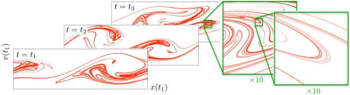
Figure 1: Snapshots of the phase-space attractor for an idealised model. The equation of motion is a one-dimensional version of Equation 4, $\dot{x}=v$, $\dot{v}=-[v-u(x,t)]/\tau_{\rm p}$, with a random velocity field $u(x,t)$ (Section 6). Shown are the positions $x(t)$ and velocities $v(t)$ of $10^{6}$ particles at different times (red dots). The magnifications illustrate fractal clustering.

Equation 4 defines a dynamical system in six-dimensional phase space. How phase-space structures stretch and contract under the dynamics is measured by the Lyapunov exponents $\lambda_{1}\geq\lambda_{2}\geq\cdots\geq\lambda_{6}$. They describe how nearby particle trajectories diverge or converge. The growth rate $\lim_{t\to\infty}t^{-1}\log[\mathscr{V}_{n}(t)/\mathscr{V}_{n}(0)]$ of the volume $\mathscr{V}_{n}(t)$ of an $n$-dimensional phase-space region is $\sigma_{n}=\lambda_{1}+\cdots+\lambda_{n}$ ($\sigma_{1}$ for distances, $\sigma_{2}$ for areas, …). The inertial dynamics of small particles in incompressible turbulence is chaotic because $\lambda_{1}>0$. At the same time, since $\sigma_{6}={\nabla_{\!\scriptsize\mbox{\boldmath$x$}}\cdot\dot{\mbox{\boldmath$x$}}+\nabla_{\!\scriptsize\mbox{\boldmath$v$}}\cdot\dot{\mbox{\boldmath$v$}}}=-{3}/\tau_{\rm p}<0$, phase-space volumes contract. In short, the dynamics of this dissipative chaotic system stretches, folds, and contracts, causing particle trajectories to converge to a phase-space attractor that evolves in time (Figure 1). Dynamical-systems theory allows to analyse this attractor, and to draw conclusions about the physical properties of the system (Sections 8–10).

Attractors of dissipative chaotic systems are fractal, not smooth. The distribution of phase-space distances $\delta w=\sqrt{|\delta\mbox{\boldmath$x$}_{t}|^{2}+\tau^{2}|\delta\mbox{\boldmath$v$}_{t}|^{2}}\big{/}\ell$ has power-law form, Prob$(\delta w<\delta)\sim\delta^{D_{2}}$ for $\delta\ll 1$, with time and length scales $\tau$ and $\ell$, and where $\delta\mbox{\boldmath$x$}_{t}$ is the separation between two nearby particles, and $\delta\mbox{\boldmath$v$}_{t}$ their relative velocity. The exponent $D_{2}$ is the fractal correlation dimension of the phase-space attractor. More generally, the attractor is characterised by a spectrum $D_{p}$ of fractal dimensions (Grassberger, 1983, Hentschel & Procaccia, 1983), defined in terms of the fraction of particles $\mathscr{M}_{\delta}(\mbox{\boldmath$x$}_{t},\mbox{\boldmath$v$}_{t},t)$ contained in a small ball of radius $\delta$ around $(\mbox{\boldmath$x$}_{t},\mbox{\boldmath$v$}_{t})$. For positive integer $p$, the $p$-th moment of $\mathscr{M}_{\delta}$ is the probability of finding $p+1$ particles within $\delta$ from each other. The average of $\mathscr{M}^{p}_{\delta}(\mbox{\boldmath$x$}_{t},\mbox{\boldmath$v$}_{t},t)$ along trajectories has power-law form in the statistically steady state, $\langle\mathscr{M}^{p}_{\delta}\rangle\sim\delta^{\xi_{p}}$ for $\delta\ll 1$. The exponents $\xi_{p}\equiv p\,D_{p+1}$ define the fractal dimensions. In analogy with multifractal turbulence models, one expects that $\xi_{p}$ are non-linear, concave functions of $p$ (Paladin & Vulpiani, 1987, Meibohm et al., 2020). This implies that the phase-space distribution is intermittent. [] Intermittent mass distributionthe probability density of $\mathscr{M}_{\delta}$ has non- Gaussian tails. This results in large fluctuations of particle separations and relative velocities (Sections 9 and 10).

[t]

5 MEASURING FRACTAL DIMENSIONS OF SPATIAL PATTERNS

The radial distribution function $g(R)$ measures the probability of finding two particles at distance $R$ in configuration space. In three spatial dimensions, the function is defined as $g(R)={(4\pi R^{2}})^{-1}\tfrac{{\rm d}}{{\rm d}R}\langle\hat{\mathscr{M}}_{R}\rangle$, and it is normalised such that $g(R)=1$ for uniformly distributed particles. When the particles form fractal clusters $g(R)$ grows as a power law $\propto R^{\hat{D}_{2}-{3}}$ at small distances, with spatial correlation dimension $\hat{D}_{2}<3$. A fractal dimension introduced by Kaplan & Yorke (1979), $\hat{D}_{KY}$, measures the dimensionality of spatial regions that neither expand nor contract. This dimension can be calculated from the spatial Lyapunov exponents. Under quite general circumstances one can show that $\hat{D}_{KY}=\hat{D}_{1}$ (Ledrappier & Young, 1988).

5.1 Multi-valued velocities and projection

To determine the spatial distribution of particles, one must project the phase-space patterns to configuration space ($x$-space). A fold of a smooth phase-space curve causes a divergence of the projected spatial density, a catastrophe or caustic just as in geometrical optics (Berry & Upstill, 1980), and in the mass distribution in the early universe (Zel’Dovich, 1970). The phase-space patterns of heavy particles in turbulence are fractal. Nevertheless their folds (fractal catastrophes, see Meibohm et al., 2020) result in large spatial particle-number densities (Crisanti et al., 1992, Martin & Meiburg, 1994, Wilkinson & Mehlig, 2005).

Between two caustics, the projection to configuration space is many-to-one (Falkovich et al., 2002). []Causticfold location of a smooth phase-space curve in configuration space. If the particles approach on different branches of the phase-space attractor (Figure 1), they can collide at high velocities, a process called sling effect by Falkovich et al. (2002). []Sling effectmechanism by which particles collide at high velocities, facilitated by caustics. In Figure 1, fold caustics are points on the $x$-axis. In reality, fold caustics are surfaces in configuration space around regions of multi-valued particle velocities. Higher-order catastrophes can occur, such as cusp catastrophes, swallow-tails, and umbilics (Berry & Upstill, 1980). As the attractor folds, caustics occur at rate $\mathscr{J}$, increasing the number of phase-space branches with different velocities. This is balanced by the contraction of the dynamics in the velocity direction, so that a steady state emerges.

Spatial distributions of particles in turbulence inherit their fractal properties from the fractal phase-space attractor. The fraction of particles $\hat{\mathscr{M}}_{\delta}(\mbox{\boldmath$x$}_{t},t)$ in a sphere of non-dimensional radius $\delta$ around $\mbox{\boldmath$x$}_{t}$ obeys $\langle\hat{\mathscr{M}}_{\delta}^{p}\rangle\sim\delta^{{p}\hat{D}_{{p}+1}}$ for $\delta\ll 1$, with spatial fractal dimension $\hat{D}_{{p}+1}$. The first moment defines the the spatial correlation dimension ${\hat{D}}_{2}$ (Section 9). For a typical projection of a generic attractor to a three-dimensional subspace, the projected correlation dimension obeys $\hat{D}_{2}=\mbox{min}\{D_{2},{3}\}$ (Hunt & Kaloshin, 1997, Bec et al., 2008). Meibohm et al. (2020) showed that this saturation of $\hat{D}_{2}$ at the spatial dimension is due to caustics, they result in a uniform particle distribution at large ${\rm St}$. Projection formulae for other fractal dimensions are not known. Settling changes fractal clustering in configuration space (Section 9), the spatial patterns become anisotropic (Bec et al., 2014, Gustavsson et al., 2014, Ireland et al., 2016b).

Particles with different Stokes numbers cluster on different fractal attractors, shifted with respect to each other (Chun et al., 2005, Bec et al., 2005, Section 9). The phase-space attractors are shifted too, affecting the relative particle-velocity distribution (Section 10).

Spatial clustering has been analysed using Voronoi tessellations of thin slices of particle positions (Monchaux et al., 2010). This provides a robust measure of particle clustering. But it does not yield information about the fractal dimensions.

6 STATISTICAL MODELS

Statistical models avoid some of the challenges posed by ab-initio simulations of particles in turbulence. The idea is to study the solutions of Equation 4 with a prescribed fluid velocity $\mbox{\boldmath$u$}(\mbox{\boldmath$x$},t)$, using mathematical analysis, statistical closure, or Monte-Carlo simulation. The goal is twofold. First, there is no other way at the moment of studying how the 10⁸ water droplets in a cubic metre of a turbulent atmospheric cloud determine its radiative properties (Schneider et al., 2017). Second, the analysis of idealised statistical models can explain the key mechanisms and non-dimensional parameters that determine the particle dynamics. [] Lagrangian fluid elementsinfinitesimal fluid elements that follow the flow like tracers.

This approach has been successful for inertialess tracer particles. Their turbulent mixing is understood using Lagrangian models, which approximate the turbulent velocity fluctuations seen by Lagrangian fluid elements (Pope, 1994). A different point of view was taken by Kraichnan (1968). He analysed how the spatial concentration $n(\mbox{\boldmath$x$},t)$ of tracer particles develops according to Equation 1, using a statistical model for the Eulerian field $\mbox{\boldmath$u$}(\mbox{\boldmath$x$},t)$. The theoretical analysis of Kraichnan’s model allows to relate the scalar concentration fluctuations to the relative motion of the tracers (Falkovich et al., 2001). [] Kraichnan modelapproximates $\mbox{\boldmath$u$}(\mbox{\boldmath$x$},t)$ as a Gaussian random field, which is white-noise in time with power-law correlations in space.

Heavy particles that do not follow the flow call for different levels of sophistication in the modelling. One can solve the Navier–Stokes equations without the particles by direct numerical simulation and integrate Equation (4) with the numerically computed $\mbox{\boldmath$u$}(\mbox{\boldmath$x$},t)$ (Riley & Patterson, 1974, Squires & Eaton, 1991, Sundaram & Collins, 1997). This method is called one-way-coupled DNS (Elgobashi, 2019). Although not ab-initio, it has significantly advanced our understanding of the problem (Brandt & Coletti, 2022).

[b]

7 MATCHING STATISTICAL MODELS TO TURBULENCE

In KS-models, a discrete set of Fourier modes $k_{n}$ is chosen to approximate the turbulent kinetic-energy spectrum $E(\mbox{\boldmath$k$})\simeq 1.5\,\varepsilon^{-2/3}|\mbox{\boldmath$k$}|^{-5/3}$ (upper and lower cutoffs are matched to $\eta$, and to the large scale $L$). Time correlations are imposed by the frequency spectrum $\omega_{n}=\omega_{0}\sqrt{k_{n}^{3}E(k_{n})}$, where $\omega_{0}$ determines the Kubo number (Voßkuhle et al., 2015). The Stokes number is not defined in terms of $\tau_{\eta}$, but using a typical wave number (Ijzermans et al., 2010), introducing an unknown factor in the definition of ${\rm St}$. The three parameters $u_{0}$, $\ell_{0}$, $\tau_{0}$ of the single-scale model are matched as follows. The magnitude of actual turbulent fluid-velocity gradients is $\sim\!\tau_{\eta}^{-1}$, and Lagrangian fluid elements separate and decorrelate on time scales $\sim\!\tau_{\eta}$. The single-scale model exhibits the same behaviour for $\tau_{0}\gg\tau_{\eta}$. In this large-${\rm Ku}$ limit, the Eulerian time scale $\tau_{0}$ does not matter, and one matches the model time-scale $\ell_{0}/u_{0}$ to the Kolmogorov time $\tau_{\eta}$ of the turbulent flow. To model single-particle statistics (Section 8), the remaining parameter is chosen as $u_{0}=\sqrt{3}u_{\rm rms}$, or equivalently $\ell_{0}=\lambda$, the Taylor microscale. For the dynamics of particle separations (Sections 9 and 10), one matches $\ell_{0}$ to the length scale where the smooth dissipation range turns into the inertial range, of the order $\ell_{0}\sim 10\eta$. For KE-models, one matches the eddy-turnover time $\tau_{\ell}$ to turbulence, as well as the correlation times $\tau_{O}$ and $\tau_{S}$ of vorticity and strain. The resulting model contains unknown higher-order structure functions of fluid-velocity differences. They are approximated in terms of two-point functions. The latter are taken from DNS (Bragg & Collins, 2014a, b). An alternative to DNS is to develop and analyse idealised models for the turbulent flucutations. Maxey & Corrsin (1986) used an ensemble of stationary cellular flows. Saffman & Turner (1956) averaged over Gaussian-distributed fluid-velocity gradients $\mathbb{A}$ of time-independent linear flows $\mbox{\boldmath$u$}(\mbox{\boldmath$x$})=\mathbb{A}\,\mbox{\boldmath$x$}$. Falkovich et al. (2007) used a one-dimensional model where $A=\partial u/\partial x$ follows a telegraph process. Another possibility is to represent $\mbox{\boldmath$u$}(\mbox{\boldmath$x$},t)$ as a sequence of non-linear velocity fields $\mbox{\boldmath$u$}_{t}(\mbox{\boldmath$x$})$ changing at random times $t$ (Pergolizzi, 2012). The most common approach, however, is to approximate the turbulent velocity by an incompressible random field. To ensure incompressibility, it is convenient to represent the fluid velocity as the curl of a random vector potential, $\mbox{\boldmath$u$}(\mbox{\boldmath$x$},t)=\mbox{\boldmath$\nabla$}\wedge\mbox{\boldmath$\Psi$}(\mbox{\boldmath$x$},t)$. The vector potential $\mbox{\boldmath$\Psi$}(\mbox{\boldmath$x$},t)$ is constructed from random spatial Fourier modes. []KS modelapproximates $\mbox{\boldmath$u$}(\mbox{\boldmath$x$},t)$ as a Gaussian random function with power-law correlations in space and time. Kinematic-simulation (KS) models (Fung et al., 1992, Ducasse & Pumir, 2009, Ijzermans et al., 2010) approximate turbulent inertial-range scaling by imposing a power-law dependence of the correlation function $\langle\Psi_{i}(\mbox{\boldmath$x$},t)\Psi_{j}(\mbox{\boldmath$x$}^{\prime},t^{\prime})\rangle$ upon $\mbox{\boldmath$x$}-\mbox{\boldmath$x$}^{\prime}$, as in the Kraichnan model. While Kraichnan’s model is white noise in time, KS models have a non-zero decay time.

To describe the particle dynamics in the dissipative range of turbulence, one can simplify the model further, keeping only a single spatial scale $\ell_{0}$. Time correlations can be generated by Ornstein-Uhlenbeck processes, resulting in components $\Psi_{j}$ of the vector field that are Gaussian distributed with zero mean and correlations (Maxey, 1987, Pinsky & Khain, 1995, Sigurgeirsson & Stuart, 2002, Bec et al., 2005, 2008, Gustavsson & Mehlig, 2016), []Single-scale modelapproximates $\mbox{\boldmath$u$}(\mbox{\boldmath$x$},t)$ as a Gaussian random function with the single spatial scale $\ell_{0}$.

$$\left\langle\Psi_{i}(\mbox{\boldmath$x$},t)\Psi_{j}(\mbox{\boldmath$x$}^{\prime},t^{\prime})\right\rangle=\mathscr{C}\,(u_{0}\,\ell_{0})^{2}\,\delta_{ij}\,\exp\big{[}-{|\mbox{\boldmath$x$}-\mbox{\boldmath$x$}^{\prime}|^{2}}/(2\ell_{0}^{2})-{|t-t^{\prime}|}/{\tau_{0}}\big{]}\,.$$ (15)

The normalisation constant $\mathscr{C}$ is chosen so that $\langle|\mbox{\boldmath$u$}|^{2}\rangle=u_{0}^{2}$. The model has two time scales: the Eulerian correlation time $\tau_{0}$ and the Kolmogorov time $\tau_{\eta}=({\rm Tr}\,\,\langle\mathbb{A}^{\sf T}\mathbb{A}\rangle)^{-1/2}$ which evaluates to $\tau_{\eta}=\ell_{0}/(u_{0}\sqrt{{5}})$. The ratio of these time scales defines the Kubo number ${\rm Ku}=\frac{u_{0}\tau_{0}}{\ell_{0}}\propto\frac{\tau_{0}}{\tau_{\eta}}$ (Wilkinson et al., 2007). In order to match the model to turbulence, one considers the limit of large Kubo numbers, where the dynamics becomes independent of $\tau_{0}$. The remaining parameters, $u_{0}$ and $\ell_{0}$, can then be matched to the relevant scales of the turbulent flow. In this case, any dependence on ${\rm Re}_{\lambda}$ is contained in the choice of $u_{0}$ and $\ell_{0}$. The model allows mathematical analysis in the limit of small but finite ${\rm Ku}$ using perturbation theory (Gustavsson & Mehlig, 2016). The white-noise limit (the limit ${\rm Ku}\to 0$ at constant ${\rm Ku}\,{\rm St}$) can be analysed using diffusion approximations (Wilkinson et al., 2007). The persistent limit of ${\rm Ku}\to\infty$ at constant ${\rm St}$ can in some cases be treated analytically (Derevyanko et al., 2007, Pergolizzi, 2012, Meibohm et al., 2023a).

The single-scale model assumes that the particle dynamics is mainly determined by the smooth part of the turbulent velocity correlation function. At large Stokes numbers or settling velocities, the inertial range may influence the particle dynamics, and this can lead to new parameter dependencies, for example on ${\rm Re}_{\lambda}$. KS models do have a range of spatial scales, but they do not account for the sweeping of small turbulent eddies by large ones. Instead, large eddies drag Lagrangian fluid elements through smaller eddies. As a consequence, fluid-velocity gradients decorrelate too quickly compared with turbulence (Voßkuhle et al., 2015). Both models have Gaussian fluid-velocity fluctuations. This means that they neglect violent fluctuations of the fluid-velocity gradients corresponding to persistent regions of anomalously high turbulent vorticity. Under which circumstances this matters is discussed in the following Sections.

Other models for dispersed multiphase flow are related to Langevin models for the Lagrangian dynamics of fluid elements (Pope, 1994). Approximate Langevin equations for inertial particles (Minier, 2016) allow to compute the distribution of $\mbox{\boldmath$x$}(t)$, $\mbox{\boldmath$v$}(t)$, and $\mbox{\boldmath$u$}(\mbox{\boldmath$x$}(t),t)$ by Monte-Carlo simulation. The models reproduce single-time, single-particle statistics, but they are not designed to describe two-point statistics such as relative particle-velocities. Multi-valued particle velocities can be represented in a heuristic fashion, by decomposing the particle velocities into two contributions, a smooth velocity field plus spatially uncorrelated fluctuations intended to represent the effect of caustics (Fevrier et al., 2005). Alternatively, one may consider models for the distribution of $\mbox{\boldmath$x$}(t)$ and $\mbox{\boldmath$v$}(t)$ alone. One can derive a kinetic equation (KE) for $P(\mbox{\boldmath$x$},\mbox{\boldmath$v$};t)$ if one assumes that the turbulent velocity fluctuations are Gaussian. Keeping only the leading terms in a moment expansion, one obtains:

$$\left\{\partial_{t}+v_{i}\partial_{x_{i}}-\tfrac{1}{\tau_{\rm p}}\partial_{v_{i}}v_{i}-\tfrac{1}{\tau_{\rm p}}\partial_{v_{i}}\left[\partial_{v_{j}}\mu_{ij}(\mbox{\boldmath$x$},t)+\partial_{x_{j}}\lambda_{ij}(\mbox{\boldmath$x$},t)-\kappa_{i}(\mbox{\boldmath$x$},t)\right]\right\}P(\mbox{\boldmath$x$},\mbox{\boldmath$v$};t)=0\,.$$ (16)

Here $\mu_{ij}$, $\lambda_{ij}$, and $\kappa_{i}$ are unknown coefficients that require closure approximations, and summation over repeated indices is implied. This approach yields accurate numerical descriptions of single-particle properties, also in spatially inhomogeneous turbulent flow (Reeks, 2021). Zaichik & Alipchenkov (2003) derived analogous equations for two-particle statistics. Such KE models can be closed using DNS results for the unknown []Closureapproximate evaluation of unknown terms in a moment expansion. [] KE modelkinetic equation for distribution of particle positions and velocities, requiring closure. coefficients (Bragg & Collins, 2014a, b), to obtain numerical results for the statistics of separations and relative velocities between heavy particles in turbulence. In Sections 9 and 10, we compare the corresponding results to those of statistical models based on Equation 15. In the white-noise limit, the kinetic equation for particle separations and relative velocities reduces to a Fokker-Planck equation, of similar form as the one-dimensional equation analysed by Gustavsson et al. (2008).

8 PREFERENTIAL SAMPLING

8.1 Maxey’s centrifuge

Heavy particles can detach from the flow, they are not Lagrangian fluid elements. This leads to a bias in the statistical properties of the fluid-velocity gradients evaluated along particle paths (Maxey, 1987), called preferential sampling. Maxey obtained an approximate equation-of-motion by expanding Equation 4 at small ${\rm St}$. When ${\rm Sv}=0$, this yields $\tfrac{{\rm d}}{{\rm d}t}\mbox{\boldmath$x$}\approx\mbox{\boldmath$v$}_{\rm p}(\mbox{\boldmath$x$},t)=\mbox{\boldmath$u$}-\tau_{\rm p}\tfrac{\rm D}{{\rm D}t}\mbox{\boldmath$u$}$. Since the effective particle-velocity field $\mbox{\boldmath$v$}_{\rm p}(\mbox{\boldmath$x$},t)$ is compressible, [] Maxey’s centrifugeparticle inertia expels heavy particles from vortices. $\mbox{\boldmath$\nabla$}\cdot\mbox{\boldmath$v$}_{\rm p}=-\tau_{\rm p}{\rm Tr}\,\mathbb{A}^{2}=-\tau_{\rm p}\big{(}{\rm Tr}\,\mathbb{S}^{2}-{\rm Tr}\,\mathbb{O}^{\sf T}\mathbb{O}\big{)}\neq 0$, he concluded that small-${\rm St}$ particles are more likely to explore the sinks of $\mbox{\boldmath$v$}_{\rm p}(\mbox{\boldmath$x$},t)$, regions of large strain and small vorticity. This centrifuge effect is illustrated in Figure 2a, showing a snapshot of particle positions together with the magnitude of vorticity $\omega\equiv\mbox{\boldmath$|$}\nabla\wedge\mbox{\boldmath$u$}(\mbox{\boldmath$x$},t)|=\sqrt{2{\rm Tr}\,\mathbb{O}^{\sf T}\mathbb{O}}$. Heavy particles tend to avoid connected regions of high vorticity of linear sizes smaller than $\sim{10\eta}$ (Section 6).

Falkovich & Pumir (2004) predicted that $\langle{\rm Tr}\,\mathbb{A}^{2}\rangle{\tau_{\eta}^{2}}\propto{\rm St}$ along particle paths. This is consistent with a perturbative analysis of the single-scale model neglecting multi-valued particle velocities, which gives $\langle{\rm Tr}\,\mathbb{A}^{2}\rangle\tau_{\eta}^{2}{\propto}{\rm St}$ for small ${\rm Ku}$ and ${\rm St}$ (Gustavsson & Mehlig, 2016). Figure 2b shows $\langle{\rm Tr}\,\mathbb{A}^{2}\rangle$ from DNS and simulations of the single-scale model. The results are qualitatively similar, but there is one important difference: the model underestimates preferential sampling (Gustavsson & Mehlig, 2016) because turbulence has more persistent regions of much larger vorticity that act as efficient centrifuges (Figure 2a). Note that the DNS results decrease more slowly than predicted by perturbation theory as ${\rm St}\to 0$. The reason for this difference is not understood. Figure 2b also shows that the centrifuge effect becomes weaker at larger ${\rm St}$. This is expected, because the history of the fluid-velocity gradients seen by the particle matters more than the gradients at the present position (Gustavsson et al., 2008, Bragg et al., 2015b). Note also that the DNS results in Figure 2b show a weak dependence on ${\rm Re}_{\lambda}$. A possible explanation is that at larger ${\rm Re}_{\lambda}$ particles are more likely to be expelled from straining regions (Ireland et al., 2016a).

\begin{overpic}[width=455.24408pt]{Fig2} \end{overpic}

Figure 2: Preferential sampling. a Heavy particles avoid vortices. Shown are DNS results for particle positions in a thin slice of three-dimensional configuration space. Different levels of gray reflect particle depth within the slice [data from Bec et al. (2014) with ${\rm St}=1$ and ${\rm Re}_{\lambda}\approx 460$]. Also shown is the magnitude $\omega$ of vorticity (see text). b Average of ${\rm Tr}\,\mathbb{A}^{2}$ along inertial-particle paths versus ${\rm St}$. DNS results from Ireland et al. (2016a) ($\scriptstyle\Box$, $\Diamond$), Bec et al. (2014) ($\scriptstyle\bigtriangleup$, $\scriptstyle\bigtriangledown$ ), data from simulations of the single-scale model (Equation 15) for ${\rm Ku}=10$ ($\bullet$), and the prediction of perturbation theory $\tau_{\eta}^{2}\langle{\rm Tr}\,\mathbb{A}^{2}\rangle\propto{\rm St}$ (solid line). c Voids in the spatial distribution of cloud droplets. Data from (Karpińska et al., 2019). Image obtained from E. Bodenschatz.

An alternative preferential-sampling mechanism was suggested by Coleman & Vassilicos (2009): at small ${\rm St}$, heavy particles cluster near points of zero fluid acceleration, where $\tfrac{{\rm D}}{{\rm D}t}\mbox{\boldmath$u$}=0$. At small Stokes numbers, this is consistent with Maxey’s small-${\rm St}$ expansion. At large ${\rm St}$, by contrast, this expansion fails, and preferential sampling of low-acceleration regions becomes negligible (Bragg et al., 2015a).

Quantifying preferential sampling in laboratory experiments is hard because one must simultaneously track particles and fluid-velocity gradients. The measurements of Gibert et al. (2012) and Petersen et al. (2019) show a certain bias towards straining regions at intermediate Stokes numbers.

8.2 Settling

Preferential sampling has a significant effect on the gravitational settling of particles in turbulence. Averaging Equation 4 leads to $\langle\mbox{\boldmath$v$}\cdot\hat{\mbox{\boldmath$g$}}\rangle=\tau_{\rm p}\,g+\langle\mbox{\boldmath$u$}\cdot\hat{\mbox{\boldmath$g$}}\rangle$, where $\tau_{\rm p}\,g$ is the Stokes settling speed in a still fluid. Maxey (1987) suggested that turbulence enhances settling, because particles expelled from vortices preferentially sample down-welling regions where $\mbox{\boldmath$u$}\cdot\hat{\mbox{\boldmath$g$}}>0$. This preferential sweeping is confirmed by DNS (Wang & Maxey, 1993, Bec et al., 2014, Rosa et al., 2016), as well as experiments (Aliseda et al., 2002, Good et al., 2014, Petersen et al., 2019).[] Preferential sweepingparticles preferentially sample down-welling regions of turbulent flow. The relative increase in settling speed is largest for settling numbers ${\rm Sv}\approx 1$, when the settling velocity is of the order of the smallest turbulent eddies. For large ${\rm Sv}$, Good et al. (2014) observed that turbulence can have the opposite effect, reducing the settling speed. What causes this reduction is not understood (Rosa et al., 2016), but model calculations using cellular flow fields confirm this behaviour  (Lillo et al., 2008, Afonso, 2008).

8.3 Large-scale preferential sampling

The mechanisms reviewed in Section 8.1 explain preferential sampling in the dissipative range of turbulence, leading to spatial patterns on scales up to $\ell_{0}\sim 10\eta$. Figure 2a shows strong preferential sampling also at much larger scales. Similar structures – termed cloud holes by Karpińska et al. (2019) – are observed in the spatial patterns of cloud droplets (Figure 2c). It is plausible that these voids are caused by rare fluctuations of turbulent vorticity, intense and persistent vortex tubes that manage to expel particles with moderate inertia.

At large Stokes numbers, inertial-range statistics may become important. The mean-squared particle velocity, for example, is of the order of $\langle v_{1}^{2}\rangle\sim u_{\rm rms}^{2}/(1+\tau_{\rm p}/\tau_{u})$, where $\tau_{u}\!\sim\!\tau_{L}\!=\!\tau_{\eta}{\rm Re}_{\lambda}/\sqrt{15}$ is the Lagrangian correlation time of the large-scale fluid velocity (Abrahamson, 1975, Ireland et al., 2016a). In other words, $\langle v_{1}^{2}\rangle$ obtains a ${\rm Re}_{\lambda}$ dependence due to large-scale motion. This effect can be accounted for by setting $u_{0}=\sqrt{{3}}\,u_{\rm rms}$ and ${\ell_{0}}\!\sim\!u_{\rm rms}\,\tau_{L}$ in the single-scale model, Equation 15. A related choice of scales is discussed in Section 9, intended to describe inertial-range clustering in terms of a scale-dependent Stokes number ${\rm St}_{L}\sim\tau_{\rm p}/\tau_{L}$. The only ${\rm Re}_{\lambda}$-dependence is contained in the choice of the time scale $\tau_{L}$.

The settling velocity of heavy particles, on the other hand, exhibits an intricate ${\rm Re}_{\lambda}$-dependence (Bec et al., 2014), that cannot be described by simply changing a time scale. The reason is preferential sampling: rapidly settling particles explore vertical fluid-velocity correlations at spatial separations much larger than the dissipation scale. The settling particles experience an effective horizontal flow that is compressible, and collect in the sinks of this flow. A Kraichnan model for the effect of large eddies on the settling speed predicts $\langle\mbox{\boldmath$v$}\cdot\hat{\mbox{\boldmath$g$}}\rangle/v_{\rm s}-1\propto{\rm Re}_{\lambda}^{3/4}{\rm Fr}^{5/2}{\rm St}^{-2}$, in good agreement with DNS (Bec et al., 2014).

9 FRACTAL CLUSTERING

9.1 Multiplicative amplification

Tracer particles in a compressible flow form fractal spatial patterns. The sum of the spatial Lyapunov exponents is negative, so that the Kaplan-Yorke dimension $\hat{D}_{\rm KY}$ is smaller than the spatial dimension (Sommerer & Ott, 1993, Falkovich et al., 2001, Toschi & Bodenschatz, 2009). In incompressible flow, tracer particles cannot cluster because the spatial Lyapunov exponents sum to zero. The infinitesimal volume $\hat{\mathscr{V}}_{3}=\mbox{det}[\mbox{\boldmath$R$}_{1},{\mbox{\boldmath$R$}_{2}},\mbox{\boldmath$R$}_{3}]$ spanned by three separation vectors $\mbox{\boldmath$R$}_{\alpha}$ between four nearby particles neither contracts nor expands.

Inertial particles cluster even in incompressible flow. To understand the mechanism, consider how $\hat{\mathscr{V}}_{3}$ changes. If the particles remain close to each other, one can show that $\hat{\mathscr{V}}_{3}(t+\delta t)=\det[\mathbb{I}+\mathbb{Z}(t)]\hat{\mathscr{V}}_{3}(t)$. Here, $\mathbb{Z}$ is the matrix of particle-velocity gradients $Z_{ij}=\partial v_{i}/\partial x_{j}$. Since the product of many random factors $\det[\mathbb{I}+\mathbb{Z}(t)]$ tends to be smaller than unity, spatial volumes contract. This amplifies local particle-number density fluctuations, resulting in spatial clustering by multiplicative amplification (Gustavsson & Mehlig, 2016).

The dynamical equation for $\mathbb{Z}$ follows from Equation 4 by differentiation, $\tfrac{\rm d}{{\rm d}t}\mathbb{Z}=(\mathbb{A}-\mathbb{Z})/\tau_{\rm p}-\mathbb{Z}^{2}$ (Falkovich et al., 2002). It must be integrated alongside the particle motion, therefore fractal clustering is determined by the history of the fluid-velocity gradients experienced by the particles (Gustavsson et al., 2008, Bragg et al., 2015b). In the white-noise limit (Section 6), fractal clustering is entirely due to multiplicative amplification (Wilkinson et al., 2007).

9.2 Correlation dimension

The spatial correlation dimension $\hat{D}_{2}$ has a straightforward interpretation in terms of the pair-correlation function, and quantifies the effect of fractal clustering on the collision rate (Section 10). Unfortunately, however, $\hat{D}_{2}$ is hard to calculate. Systematic perturbation expansions for the spatial correlation dimension are known only for special cases, such as the white-noise limit. To make matters worse, the perturbation series diverge asymptotically. In addition, it appears that the perturbation theory misses non-analytical contributions proportional to the rate of caustic formation (Gustavsson et al., 2015).

\begin{overpic}[width=426.79134pt]{Fig3} \end{overpic}

Figure 3: Fractal clustering. a Correlation dimension for identical particles for ${\rm Sv}=0$. Spatial $\hat{D}_{2}$ (large symbols), phase-space $D_{2}$ (small symbols) versus ${\rm St}$. DNS results: ${\rm Re}_{\lambda}=89$ (Bhatnagar et al., 2018), ${\rm Re}_{\lambda}=88$ (Bragg & Collins, 2014a), ${\rm Re}_{\lambda}=65,185$ (Bec et al., 2007), ${\rm Re}_{\lambda}=400$ (Bec et al., 2010). Model predictions: KE-model, evaluated by Bragg & Collins (2014a) using DNS for the unclosed terms (blue,$\blacklozenge$), simulations of the single-scale model (SSM, Equation 15) for ${\rm Ku}=10$ (red, $\bullet$ and $\bullet$), together with a fit to the small-${\rm St}$ asymptote (solid line). Also shown are simulations of the KS-model (Ijzermans et al., 2010) (green, $\blacksquare$), see text. Small-${\rm St}$ theory of Chun et al. (2005) evaluated by Bragg & Collins (2014a) using DNS for the unclosed terms (magenta, $\blacktriangle$). Experimental data extracted from panel b by fitting the data in the range $1\leq R/\eta\leq 10$ ($\star$). b Pair correlation functions $g(R)$ for polydisperse suspensions of droplets in air turbulence. Laboratory experiments (Saw et al., 2012), symbols, compared with predictions of single-scale model (SSM) ${\rm Ku}=10$ and $\ell_{0}/\eta=20$. First: for particles of two different sizes (dashed lines) with $\overline{{\rm St}}\sim 0.11,\theta\sim 0.91$; $\overline{{\rm St}}\sim 0.19,\theta=0.53$; $\overline{{\rm St}}\sim 0.4,\theta=0.37$; $\overline{{\rm St}}\sim 0.7,\theta=0.43$, read off from Fig. 7 in Saw et al. (2012). The average Stokes number is defined as $\overline{{\rm St}}=\overline{\tau}_{\rm p}/\tau_{\eta}$, where $\overline{\tau}_{\rm p}$ is the harmonic mean of the different Stokes times, see (Meibohm et al., 2017). Second: distribution of particle sizes extracted from their Fig. 3 (solid lines). c Effect of settling, $\hat{D}_{2}$ for different values of ${\rm Fr}$, DNS results from Bec et al. (2014), single-scale model (SSM) for ${\rm Ku}=10$ and $\ell_{0}/\eta=10$. d Inertial-range clustering, pair-correlation function $g(R)$ versus $R$ for ${\rm St}=1$. DNS at ${\rm Re}_{\lambda}=597$ (Ireland et al., 2016a), ${\rm Re}_{\lambda}=460$ (Bec et al., 2014), ${\rm Re}_{\lambda}=328$ (Ariki et al., 2018), and ${\rm Re}_{\lambda}=227$ (Ray & Collins, 2011). Single-scale model for ${\rm Ku}=10$ and $\ell_{0}/\eta=20$, and small-$R$ asymptote of $g(R)$, solid line (Section 4).

Figure 3a shows DNS measurements of $\hat{D}_{2}$ for different ${\rm Re}_{\lambda}$. Also shown are results of model calculations: numerical evaluations for the KE-model carried out by Bragg & Collins (2014a) using DNS for the unclosed terms, for the single-scale model (Equation 15), and for the KS model (Ijzermans et al., 2010). As pointed out in Section 6, the definition of the Stokes number for the KS-model contains an unknown factor. Here we simply rescaled ${\rm St}$ for the KS-model data (by a factor of $1.4$) to fit the location of the minimum in the DNS data in Figure 3a. Overall, we observe good agreement between model and DNS results. In particular, $\hat{D}_{2}$ depends only weakly on ${\rm Re}_{\lambda}$. This is expected, because $\hat{D}_{2}$ characterises the small-$R$ asymptote of $g(R)$, dominated by particle pairs that have spent a long time together at small relative velocities, but only the tails of the relative-velocity distribution are sensitive to ${\rm Re}_{\lambda}$. Therefore the small-$R$ behaviour of $g(R)$ is insensitive to ${\rm Re}_{\lambda}$-corrections. Figure 3a demonstrates that fractal clustering is strongest at ${\rm St}\approx 1$, as expected, because turbulent fluctuations affect the particles most when $\tau_{\rm p}$ and $\tau_{\eta}$ are comparable.

The largest deviations between model and DNS results are observed at small Stokes numbers. When ${\rm St}\ll 1$, one may replace the inertial-particle dynamics by advection in an effective velocity field $\mbox{\boldmath$v$}_{\rm p}(\mbox{\boldmath$x$},t)$ with ${\rm St}$-dependent compressibility (Section 8). This suggests that $3-\hat{D}_{2}\propto{\rm St}^{2}$ (Balkovsky et al., 2001, Elperin et al., 2002). Chun et al. (2005) came to the same conclusion, expanding the relative-particle dynamics for small ${\rm St}$. There is, however, no agreement on the numerical prefactor. An improved version of the small-${\rm St}$ theory by Chun et al. (2005) is also shown in Figure 3a, evaluated by (Bragg & Collins, 2014a) using DNS for the unclosed terms. The result is consistent with a ${\rm St}^{2}$-dependence, as predicted by perturbative analysis of the single-scale model (Gustavsson & Mehlig, 2016). But the DNS results are not. The reason for this discrepancy is unclear.

A large-deviation argument indicates that $3-\hat{D}_{2}=2(3-\hat{D}_{\rm KY})$ at small ${\rm St}$ (Fouxon, 2011). The same result holds in the white-noise limit (Gustavsson et al., 2015, Gustavsson & Mehlig, 2016). DNS results are consistent with this prediction (Bec et al., 2006, 2007, Calzavarini et al., 2008).

Regarding the phase-space correlation dimension $D_{2}$, we observe good overall agreement between DNS and model simulations (Figure 3a), although small differences at large ${\rm St}$ remain unexplained. We also see that $\hat{D}_{2}=\min\{D_{2},3\}$, consistent with the projection formula discussed in Section 4. [] Caustics and $\hat{D}_{2}$caustics explain that the spatial correla- tion dimension $\hat{D}_{2}$ equals the spatial di- mension for ${\rm St}\!>\!{\rm St}_{\rm c}$.

Figure 3b shows the experimental data of Saw et al. (2012) for $g(R)$, averaged over particle sizes, and results of simulations of the single-scale model, in good agreement with experiments. Averaging over different particle sizes reduces the local slope ${\rm d}\log g(R)/{\rm d}\log R$, reducing clustering. This could explain why experimental data (with size dispersion) display a larger value of $\hat{D}_{2}$ than observed in DNS (Figure 3a). Larsen et al. (2018) observed spatial clustering of cloud droplets in the dissipation range. Their results for $g(R)$ are broadly consistent with the model predictions: below $R\sim\ell_{0}$, $g(R)$ increases as $R$ decreases. However, since the Stokes numbers are very small (${\rm St}\approx 10^{-2}$), the clustering is so weak that its effect on the collision rate (Section 10) is negligible. []Size dispersionbidisperse sus- pensions contain particles of two different sizes (with different Stokes numbers, ${\rm St}_{1}$ and ${\rm St}_{2}$). Polydisperse suspensions involve a distribution of many different sizes.

Settling affects fractal clustering, because settling changes how particles sample fluid-velocity gradients. Since gravity breaks the rotational symmetry, clustering becomes anisotropic (Bec et al., 2014, Gustavsson et al., 2014), so that the pair correlation depends on the angle $\varphi$ between $g$ and $\mbox{\boldmath$\hat{R}$}=\mbox{\boldmath$R$}/R$. This affects only the prefactor, not the exponent: $g(R)=C(\varphi)R^{\hat{D}_{2}-{3}}$ (Bhatnagar, 2020). Figure 3c shows $\hat{D}_{2}$ versus ${\rm St}$ for different values of the settling number, for DNS and model simulations. Overall we observe good agreement. At small ${\rm St}$, fractal clustering decreases slightly as the effect of gravity increases (smaller ${\rm Fr}$). But at large ${\rm St}$, settling increases clustering by multiplicative amplification – rapidly settling particles experience the flow as white noise (Bec et al., 2014, Gustavsson et al., 2014). Note that the correlation dimension depends non-monotonically on ${\rm Fr}$ in this regime.

Lu et al. (2010) measured the effect of electrical charges on spatial clustering of droplets in turbulence. They determined $g(R)$ for highly charged droplets of equal parity, and found that the resulting electrostatic interactions affect the pair correlation function $g(R)$ at length scales below $R/\eta\sim 4$, for ${\rm St}=0.3$ and ${\rm Re}_{\lambda}=80$. At present there is no systematic study of how the spatial clustering depends on the amount of charge, on ${\rm St}$, and on ${\rm Re}_{\lambda}$.

9.3 Inertial-range clustering

The fractal dimensions $\hat{D}_{\rm KY}$ and $\hat{D}_{2}$ discussed above measure small-scale fractal clustering in the dissipative range of turbulence. In turbulent flow, spatial clustering is observed not only in the dissipative range but also in the inertial range. However, as seen from Figure 3d, the radial distribution function $g(R)$ no longer behaves as a power-law when $R\gg\eta$. In the inertial range, the turnover time $\tau_{{R}}=({R}^{2}/\varepsilon)^{1/3}$ depends on the spatial scale ${R}$. Based on this observation, Falkovich et al. (2003) suggested that the radial distribution function behaves as $\log g(R)\propto{\rm St}_{R}^{2}\sim\tau_{\rm p}^{2}/R^{4/3}$ (Balkovsky et al., 2001). The scale-dependent Stokes number arises naturally in white-noise models. Simulations of the Kraichnan model yield $\log g(R)/\log R\simeq\hat{D}_{2}({\rm St}_{R})-3\propto{\rm St}_{R}^{2}$ (Bec et al., 2008). To which extent time correlations change this picture is unclear. KS models cannot answer this question, because they do not account for sweeping. In particular, the degree of large-scale clustering obtained in KS-model simulations depends on the parameter $\omega_{0}$, that is on the Kubo number (Section 6), see Chen et al. (2006). There is numerical evidence for the scaling $\log g(R)\propto R^{-4/3}$ from DNS (Bragg et al., 2015a, Ariki et al., 2018). KE-models yield the same inertial-range scaling, but they do not capture the Stokes-number dependence (Bragg et al., 2015a).

An alternative picture was proposed by Bec et al. (2007). They argued and observed in DNS that $g(R){R^{2}}$ depends on a non-dimensional ejection rate $\Gamma(R,\tau_{\rm p})\propto u_{\rm rms}\varepsilon^{1/3}\tau_{\rm p}/R^{5/3}$. How to reconcile this behaviour with the above ${\rm St}_{R}$-scaling remains an open question. The function $\Gamma(R,\tau_{\rm p})$ prescribes the scale-dependence not only of $g(R){R^{2}}=\tfrac{\rm d}{{\rm d}R}\langle\hat{\mathscr{M}}_{R}\rangle$, but of the whole probability distribution $p(\hat{\mathscr{M}}_{R})$. In DNS, deviations from a uniform distribution are significant in the two tails of this distribution. The form of the tails is explained by the statistical ejection model of Bec & Chétrite (2007). They found that $p(\hat{\mathscr{M}}_{R})\propto\hat{\mathscr{M}}_{R}^{\alpha}$ at small $\hat{\mathscr{M}}_{R}$, and $\propto\exp(-c\,\hat{\mathscr{M}}_{R}\log\hat{\mathscr{M}}_{R})$ for large $\hat{\mathscr{M}}_{R}$, where $\alpha$ and $c$ depend only on $\Gamma(R,\tau_{\rm p})$.

A certain form of scale invariance is recovered in the distribution of large void sizes. DNS of two-dimensional (Boffetta et al., 2004, Goto & Vassilicos, 2006) and three-dimensional turbulence (Yoshimoto & Goto, 2007), as well as experimental data (Sumbekova et al., 2017) suggest that the probability distribution of very large void sizes behaves as a power-law. However, different authors obtain different power-law exponents.

10 CAUSTICS AND RELATIVE VELOCITIES

\begin{overpic}[width=426.79134pt]{Fig4} \end{overpic}

Figure 4: Relative velocities. a Multi-valued particle velocities (red and blue arrows) from a thin slice of a three-dimensional DNS (Bec et al., 2014). The two colours distinguish two particle clouds with different histories. b Experimental observation of two nearby particle pairs (red and blue) with anomalously large relative velocity, adapted from Fig. 2 in Bewley et al. (2013) with permission. c Particle-velocity structure function $S_{2}(R)$ versus $R$ for ${\rm Sv}=0$. DNS from Bec et al. (2010) [${\rm Re}_{\lambda}=400$, small empty symbols], and Bragg & Collins (2014b) [${\rm Re}_{\lambda}=597$, large empty symbols], single-scale model (SSM, Equation 15) with ${\rm Ku}=10$ and $\ell_{0}/\eta=15$ (small filled symbols), ${\rm St}\!=\!0$-result from Equation 15 (solid red line), small-$R$ scaling prediction 17 (lines), and KE-model predictions evaluated by Bragg & Collins (2014b) (large filled symbols) c Joint distribution of $R$ and $V_{R}$ from DNS, adapted from Fig. 3(b) in (Bhatnagar et al., 2018). The matching line $V_{R}\sim z^{\ast}R$ (see text) is shown as a thick solid line.

Particle inertia causes large fluctuations of relative particle velocities $\mbox{\boldmath$V$}=\mbox{\boldmath$v$}_{2}-\mbox{\boldmath$v$}_{1}$ in turbulence. The reason is that phase-space manifolds fold at caustic singularities, resulting in multi-valued particle velocities (Section 4). This is illustrated in Figure 4a, which shows inertial-particle velocities in a thin slice of configuration space. The two colours distinguish two particle clouds that move on different branches of the phase-space attractor. Figure 4b shows measured droplet trajectories in turbulent air (Bewley et al., 2013). As in panel a, the two colours distinguish particle pairs originating from different regions in phase space, allowing the pairs to pass close to each other at anomalously large relative velocities.

10.1 Rate of caustic formation

The rate of caustic formation $\!\mathscr{J}\!$ depends sensitively on ${\rm St}$, because dimensional analysis shows that the required strain for a caustic to form is proportional to ${\rm St}^{-1}$. At small ${\rm St}$, the rate of caustic formation is therefore determined by the tails of the turbulent velocity-gradient distribution (Meibohm et al., 2023b, Bätge et al., 2022). In the white-noise limit, diffusion approximations for the Gaussian single-scale model yield $\scalebox{0.75}[1.0]{$-$}\log(\mathscr{J}\!\tau_{\rm p})\propto({\rm Ku}\,{\rm St})^{-1}$ for ${\rm Ku}\,{\rm St}\ll 1$ (Wilkinson & Mehlig, 2005). In the persistent limit of the Gaussian model, the rate has a different form, $\scalebox{0.75}[1.0]{$-$}\log(\mathscr{J}\!\tau_{\rm p})\propto{\rm St}^{-2}$ (Falkovich et al., 2002, Derevyanko et al., 2007). Kinematic simulations by Ducasse & Pumir (2009) and DNS by Bhatnagar et al. (2022) yield $\scalebox{0.75}[1.0]{$-$}\log(\mathscr{J}\!\tau_{\rm p})\propto{\rm St}^{-1}$. In general, one expects $\scalebox{0.75}[1.0]{$-$}\log(\mathscr{J}\!\tau_{\rm p})\propto{F}({\rm St})$ where ${F}\to\infty$ as ${\rm St}\to 0$. The form of ${F}$ depends on the tails of the velocity-gradient distribution. The key point is nevertheless that caustics form at small ${\rm St}$, leading to multivalued particle velocities. For very small ${\rm St}$, however, phase-space contraction reduces the effect of caustics, when $\mathscr{J}\!\tau_{\rm p}\ll 1$. Voßkuhle et al. (2014) concluded that caustics have a significant effect on the collision rate for ${\rm St}{\gtrsim}0.3$. Exceptions to this rule are model flows with bounded fluid-velocity gradients, where $\!\mathscr{J}\!$ vanishes below a certain Stokes number (Ijzermans et al., 2010).

[] Caustic formationFold caustics form when the particle- velocity gradients diverge, equivalently when the infini- tesimal volume $\hat{\mathscr{V}}_{3}$ collapses. Perrin & Jonker (2014) found that caustics tend to occur in regions of large turbulent strain. Meibohm et al. (2021, 2023a) explained this by computing the optimal path to caustic formation in the persistent limit, at weak particle inertia, and ${\rm Sv}=0$.

10.2 Relative particle velocities

Völk et al. (1980) estimated the relative velocities between identical particles as $\langle V_{R}^{2}\rangle\sim\varepsilon\tau_{\rm p}$. Related expressions for particles with different sizes were suggested by Mizuno et al. (1988). These estimates fail to describe the relative particle-velocities at small spatial separations, because the derivation ignores the dissipation-range dynamics (Pan & Padoan, 2010). DNS results indicate that the relative-velocity moments $m_{n}(R)\equiv\int_{-\infty}^{\infty}{\rm d}V_{R}|V_{R}|^{p}P(R,V_{R})$ depend sensitively on both $R$ and ${\rm St}$. Figure 4c shows DNS results for the relative particle-velocity structure function $S_{2}(R)\equiv m_{2}(R)/m_{0}(R)$. Also shown are results of model calculations, for the KE model as evaluated by (Bragg & Collins, 2014b), and for the single-scale model based on Equation 15. For advected particles (${\rm St}=0$), $S_{2}(R)\propto R^{2}$ in the smooth dissipative range. Particle inertia enhances the relative particle velocities, more so at smaller separations. The single-scale model describes this behaviour well, although the weak dependence on ${\rm Re}_{\lambda}$ seen for DNS is not captured by the model. The KE-model works well at ${\rm St}=3$, but fails at smaller values of the Stokes number. Bragg & Collins (2014b) suggest that this may be due to Gaussian decoupling approximations used in evaluating the model (Section 6).

The structure function exhibits anomalous scaling at small $R$, $S_{n}(R)\sim R^{\zeta_{n}}$. Gustavsson & Mehlig (2014) derived an approximate theory for the exponents $\zeta_{n}$ by matching the tails of the joint distribution $P(R,V_{R})$ at $|V_{R}|=z^{\ast}R$, with matching scale $z^{\ast}\propto\tau_{\rm p}^{-1}$ (Figure 4d). Recognising that $P(R,V_{R})$ must have algebraic large-$V_{R}$ tails at small $R$, determined by the phase-space correlation dimension $D_{2}$ (Section 4), one finds

$$m_{n}(R){\ \simeq\ }b_{n}({\rm St})(R/\eta)^{p+D_{2}-1}+c_{n}({\rm St})(R/\eta)^{{2}}$$ (17)

for small separations $R$. Equation 17 predicts that $m_{0}(R)$ is proportional to $R^{\mbox{\scriptsize min}\{D_{2},{3}\}-1}$ for small enough $R$. The scaling of the radial distribution function $g(R)=m_{0}(R)/R^{2}{\propto}R^{\hat{D}_{2}-{3}}$ implies that $\hat{D}_{2}=\mbox{min}\{D_{2},{3}\}$ (Sections 4 and 9). Using this scaling of $m_{0}(R)$, Equation 17 yields a bifractal law for the scaling exponents of the structure functions $S_{n}(R)$, namely $\zeta_{n}=\mbox{min}\{n,3-{{\hat{D}}}_{2}{({\rm St})}\}$ for $n>0$, consistent with the DNS results for $n=2$ shown in Figure 4c. Note that the saturation of $\zeta_{n}$ at large $n$ is a consequence of caustic singularities. Analogous behaviour is observed in Burgers turbulence, where the singularities are shocks. Note also that Simonin et al. (2006) suggested that $S_{2}(R)$ approaches a constant as $R\to 0$, reflecting random uncorrelated motion (Section 6). For $n>0$, this is true only when ${\rm St}$ is so large that $D_{2}>3$. [] Bifractal scalingThe scaling exponents of structure functions equal $\zeta_{n}\!=\!h_{1}n$ for $n\!<\!n_{\star}$, and $\zeta_{n}\!=\!h_{2}n\!+\!(h_{1}\!-\!h_{2})n_{\star}$ for $n\!>\!n_{\star}$. Scaling laws of this kind arise in the $\beta$-model for turbulent intermittency and in Burgers turbulence (Frisch, 1995). For the bifractal law corresponding to Equation 17, $h_{2}=0.$

The two terms on the r.h.s. of Equation 17 correspond to different histories of the relative dynamics. The first term is a smooth contribution, it comes from particles that stayed together in the past because they approached along the same phase-space branch. The second is a singular contribution, corresponding to particles that followed different phase-space branches (Figure 1). Its $R$-dependence, $\propto R^{2}$, reflects the uniform distribution of nearby particles that came from far apart with uncorrelated initial conditions.

There is no consensus regarding the particle relative-velocity distribution. It has been modeled as lognormal (Carballido et al., 2010), or with stretched exponential tails (Pan et al., 2014b). The matching ansatz outlined above yields $P(R,V_{R})R^{{2}-D_{2}}=f(V_{R}/R)$ for small distances, with $f(y)\approx{\rm min}\{y,y^{D_{2}-{4}}\}$. DNS results (Perrin & Jonker, 2015, Bhatnagar et al., 2018) at small ${\rm Re}_{\lambda}$ support this prediction. Saw et al. (2014) measured $P(R,V_{R})$ for water droplets in air turbulence. Their results do not show algebraic tails, likely because $R/\eta$ is too large. Measurements of Hammond & Meng (2021) with hollow glass spheres show much broader distributions than those of Saw et al. (2014), although their experiments explored similar parameter ranges. When the Stokes number is large enough, the analysis of Gustavsson et al. (2008) suggests that relative velocities are determined by the history of inertial-range fluctuations, resulting in $P(R,V_{R})\propto\exp\{-[V_{R}^{2}/(\tau_{\rm p}\varepsilon)]^{2/3}\}$. This is consistent with the results of Pan & Padoan (2010, 2013).

Bhatnagar (2020) concluded that settling does not change the relative dynamics very much, for identical particles. In poly-disperse suspensions, by contrast, settling is expected to have a stronger effect on the relative velocities.

For ${\rm Sv}=0$, the effect of size dispersion upon the distribution of $V_{R}$, is discussed by Pan et al. (2014a). In essence, particles with different Stokes numbers tend to have larger relative velocities. Meibohm et al. (2017) show that $S_{n}(R)$ approaches a constant for $R<R_{\theta}\propto\theta$ with $\theta{=|{\rm St}_{1}-{\rm St}_{2}|/({\rm St}_{1}+{\rm St}_{2})}$, causing an enhancement of the collision rate (Section 10.3).

Electrostatic charges affect the relative particle velocities (Alipchenkov et al., 2004, Lu & Shaw, 2015), but it is not yet clear how electrostatic interactions modify the relative-velocity theory reviewed above.

10.3 Models for the collision rate

Saffman & Turner (1956) computed how turbulence accelerates collisions between small cloud droplets. They assumed that the droplets follow the flow (${\rm St}=0$) and that they are uniformly distributed. Linearising the fluid velocity, assuming time-independent gradients, Saffman & Turner (1956) averaged over the gradients to obtain $\mathscr{R}_{\rm ST}=C_{1}n_{0}(a_{1}+a_{2})^{3}/\tau_{\eta}$. Comparing with the collision rate for droplets settling in a quiescent fluid, $\mathscr{R}_{g}\simeq n_{0}v_{s}(a_{1}+a_{2})^{2}$ with settling speed $v_{s}=\tfrac{2\varrho_{\rm p}}{9\varrho_{\rm f}{\nu}}|a_{2}^{2}-a_{1}^{2}|g$, leads to two conclusions: $\mathscr{R}_{\rm ST}$ dominates for similar-sized droplets, and it increases proportional to the turbulent shear rate.

To determine the effect of particle inertia, Sundaram & Collins (1997) integrated Equation 4 for fluid velocities obtained from turbulent DNS. They found that the collision rate

$$\mathscr{R}({{\rm St}}) =-n_{0}\lim_{R\to a_{1}+a_{2}}\int_{-\infty}^{0}\!{\rm d}V_{R}\,V_{R}\,P(R,V_{R})$$ (18)

with number density $n_{0},$ depends sensitively on the Stokes number. For identical particles this is explained by the fact that caustics allow for large relative velocities, and that the rate of caustic formation depends sensitively on ${\rm St}$. A model for the ${\rm St}$-dependence follows from Equation 17, using $\mathscr{R}({{\rm St}})\approx\tfrac{1}{2}m_{1}(2a)$. This gives $\mathscr{R}({{\rm St}})\approx\mathscr{R}_{{\rm smooth}}+\mathscr{J}({\rm St})\mathscr{R}_{\rm kin}$ (Falkovich et al., 2002). Equation 17 implies that $\mathscr{R}_{{\rm smooth}}\propto a^{\hat{D}_{2}}$, and $\mathscr{R}_{\rm kin}\propto a^{2}$, the collision rate in the kinetic limit (Abrahamson, 1975). The second term dominates for small particles and large enough ${\rm St}$. This occurs already for ${\rm St}>0.3$ (Voßkuhle et al., 2011, 2014). [] Hydrodynamic interactionsfor two nearby particles, the presence of the second particle changes the fluid velocity seen by the first one, causing them to interact. [] Collision efficiencyaccounts for the effect of hydrodynamic interactions on the collision rate.

Some authors write $\mathscr{R}({{\rm St}})\!=\!\tfrac{1}{2}g(2a)\langle|V_{R}|\rangle_{R=2a}$ (Hammond & Meng, 2021), in terms of the average $\langle\cdot\rangle_{R=2a}$ conditioned on the particle separation at contact. This does not mean that spatial clustering and relative velocities contribute in a multiplicative fashion, because $\langle|V_{R}|\rangle_{R=2a}$ equals $m_{1}(2a)/m_{0}(2a)=m_{1}(2a)/[(2a)^{2}g(2a)]$, so the factor $g(2a)$ cancels out, see Fig. 9(d)–(f) in (Nair et al., 2022). Equation 17 shows that the collision rate for identical particles depends on these two effects additively. Particle-size differences increase the collision rate between small particles because they increase their relative velocity at separations smaller than $R_{\theta}$, where $S_{2}(R)$ approaches a constant (Section 10.2). Pan & Padoan (2014) discuss in detail how size dispersion competes with particle inertia in determining $\mathscr{R}$.

The models described above neglect hydrodynamic interactions, which make it harder for the particles to approach (and to separate). In order to determine whether the particles collide or not, one must also account for the fact that hydrodynamics breaks down when the distance between the particle surfaces is smaller than the mean-free path of the fluid (Sundararajakumar & Koch, 1996). For water droplets in air, this changes the interplay between $\mathscr{R}({{\rm St}})$ and $\mathscr{R}_{g}$, and reduce the overall collision rate (Dhanasekaran et al., 2021).

Hydrodynamic interactions can be incorporated in independent-particle models in a heuristic fashion, by writing the collision rate as $e_{\rm c}\,\mathscr{R}({{\rm St}})$ (Pinsky et al., 1999, 2007, Devenish et al., 2012, Pumir & Wilkinson, 2016), where $e_{\rm c}$ is a collision efficiency intended to account for hydrodynamic interactions. Klett & Davis (1973) realised that the collision efficiency of similar-sized settling droplets depends strongly on ${\rm Re}_{p}$, simply because identical droplets do not even approach each other for ${\rm Re_{\rm p}}=0$. Klett & Davis (1973) and later studies (Pinsky et al., 2007, Wang et al., 2008) accounted for hydrodynamic interactions by perturbation theory in $a/R$. This describes the droplet dynamics at separations of the order of several droplet radii (Magnusson et al., 2022), but it does not allow to compute the collision efficiency reliably. Studies resolving close droplet approaches were performed only for ${\rm St}=0$ (Dhanasekaran et al., 2021, Dubey et al., 2022). In summary, it is not understood how the collision efficiency depends on ${\rm Re}_{p}$, ${\rm St}$, and ${\rm Sv}$.

Recent experiments (Yavuz et al., 2018, Bragg et al., 2022) measuring spatial clustering of small particles in turbulence show that the pair correlation function $g(R)$ is large at very small separations, much larger than predicted by the theories summarised in Section 9. The mechanisms for this strong clustering at very small scales remain to be understood.

[SUMMARY POINTS]

1. Statistical models provide a qualitative understanding of the phase-space dynamics of particles in turbulence, allowing to single out aspects of the dynamics that are sensitive to details of the turbulent flow. In certain cases, statistical models can be analysed systematically using dynamical-systems and perturbation theories, making it possible to gain valuable insight into key mechanisms and parameters.

2. Statistical models explain that dissipative-range spatial clustering of particles in turbulence is determined by the history of the flow encountered by the particles. To predict small-scale clustering in a quantitative fashion, one must therefore take into account that this history is biased by preferential sampling of certain flow regions. Additionally, settling alters the way in which the particles sample the flow. Specifically, settling decreases spatial clustering for small particle inertia, and increases clustering for large inertia.

3. Caustic singularities result in multi-valued particle velocities, causing continuum configuration-space descriptions to fail. Caustic formation depends sensitively on the Stokes number, at small particle inertia, as only extreme fluctuations of turbulent strain allow particles to detach from the flow. The models show that this sensitivity exists in any flow, but the specifics depend on the non-universal tails of the distribution of fluid-velocity gradients. The models also explain that caustics are responsible for the anomalous scaling of the particle-velocity structure functions, describing large collision velocities.

4. Statistical models predict which properties of the inertial-particle dynamics depend on the Reynolds number of the turbulent flow and which do not. For instance, fluctuations of particle separations and relative velocities depend only weakly on the Reynolds number. This prediction is borne out by DNS and experiments, when settling speed and particle inertia are sufficiently small to ignore inertial-range fluctuations.

[FUTURE QUESTIONS]

1. Many uncertainties remain regarding the hydrodynamic forces and torques on small particles in turbulence, concerning the effect of convective fluid inertia, in particular upon added-mass, history, and lift forces.

2. While the moments of relative velocities of heavy particles in turbulence are well understood at small spatial separations, their distribution is not. To make progress, it is necessary to formulate and analyse non-Gaussian statistical models.

3. The relative dynamics of strongly inertial particles explores the inertial range of turbulence. This can give rise to intricate dependencies of preferential sampling and relative particle velocities on the Reynolds number of the carrier flow, that remain to be understood. Formulating statistical models that consistently describe how the large-scale fluid motion affects smaller scales remains a challenge.

4. Natural flows tend to be inhomogeneous and anisotropic, simply because they contain boundaries. It is an open question how to model the effect of large-scale structures – such as mean flow gradients – on the small-scale dynamics.

5. To predict particle collision rates in turbulence, it is necessary to incorporate interactions into statistical models, including not only hydrodynamic but also electrostatic interactions. The challenge is to find reliable models for the collision efficiency that account for particle and fluid inertia, the breakdown of hydrodynamics below the mean free path, droplet deformation, and van-der-Waals interactions.

6. For non-spherical particles, translation and rotation are coupled. Developing statistical models for their collisions requires extending the position-velocity phase space to orientations and angular velocities, and to model hydrodynamic interactions between non-spherical inertial particles.

DISCLOSURE STATEMENT

The authors are not aware of any affiliations, memberships, funding, or financial holdings that might be perceived as affecting the objectivity of this review.

References

- Abrahamson (1975) Abrahamson J. 1975. Collision rates of small particles in a vigorously turbulent fluid. Chem. Eng. Sci. 30:1371–1379
- Afonso (2008) Afonso MM. 2008. The terminal velocity of sedimenting particles in a flowing fluid. J. Phys. A 41:385501
- Alipchenkov et al. (2004) Alipchenkov VM, Zaichik LI, Petrov OF. 2004. Clustering of charged particles in isotropic turbulence. High Temperature 42:919–927
- Aliseda et al. (2002) Aliseda A, Cartellier A, Hainaux F, Lasheras JC. 2002. Effect of preferential concentration on the settling velocity of heavy particles in homogeneous isotropic turbulence. J. Fluid Mech. 468:77–105
- Ariki et al. (2018) Ariki T, Yoshida K, Matsuda K, Yoshimatsu K. 2018. Scale-similar clustering of heavy particles in the inertial range of turbulence. Phys. Rev. E 97:033109
- Balachandar & Eaton (2010) Balachandar S, Eaton J. 2010. Turbulent dispersed multiphase flow. Annu. Rev. Fluid Mech. 42:111–133
- Balkovsky et al. (2001) Balkovsky E, Falkovich G, Fouxon A. 2001. Intermittent distribution of inertial particles in turbulent flows. Phys. Rev. Lett. 86:2790–2793
- Bätge et al. (2022) Bätge T, Fouxon I, Wilczek M. 2022. Quantitative prediction in turbulence at high reynolds numbers. arxiv:2208.05384
- Bec et al. (2006) Bec J, Biferale L, Boffetta G, Cencini M, Musacchio S, Toschi F. 2006. Lyapunov exponents of heavy particles in turbulence. Phys. Fluids 18:091702
- Bec et al. (2007) Bec J, Biferale L, Cencini M, Lanotte A, Musacchio S, Toschi F. 2007. Heavy particle concentration in turbulence at dissipative and inertial scales. Phys. Rev. Lett. 98:084502
- Bec et al. (2010) Bec J, Biferale L, Cencini M, Lanotte A, Toschi F. 2010. Intermittency in the velocity distribution of heavy particles in turbulence. J. Fluid Mech. 646:527–536
- Bec et al. (2005) Bec J, Celani A, Cencini M, Musacchio S. 2005. Clustering and collisions of heavy particles in random smooth flows. Phys. Fluids 17:073301
- Bec et al. (2008) Bec J, Cencini M, Hillerbrand R, Turitsyn K. 2008. Stochastic suspensions of heavy particles. Physica D 237:2037–2050
- Bec & Chétrite (2007) Bec J, Chétrite R. 2007. Toward a phenomenological approach to the clustering of heavy particles in turbulent flows. New J. Phys. 9:77
- Bec et al. (2014) Bec J, Homann H, Sankar Ray S. 2014. Gravity-driven enhancement of heavy particle clustering in turbulent flow. Phys. Rev. Lett. 112:184501
- Berry & Upstill (1980) Berry M, Upstill C. 1980. IV Catastrophe optics: Morphologies of caustics and their diffraction patterns. In Progress in optics, ed. E Wolf, vol. 18. Elsevier, 257–346
- Bewley et al. (2013) Bewley GP, Saw EW, Bodenschatz E. 2013. Observation of the sling effect. New J. Phys. 15:083051
- Bhatnagar (2020) Bhatnagar A. 2020. Statistics of relative velocity for particles settling under gravity in a turbulent flow. Phys. Rev. E 101:033102
- Bhatnagar et al. (2018) Bhatnagar A, Gustavsson K, Mitra D. 2018. Statistics of the relative velocity of particles in turbulent flows: Monodisperse particles. Phys. Rev. E 97:023105
- Bhatnagar et al. (2022) Bhatnagar A, Pandey V, Perlekar P, Mitra D. 2022. Rate of formation of caustics in heavy particles advected by turbulence. Philos. Trans. Royal Soc. A 380:20210086
- Birnstiel et al. (2016) Birnstiel T, Fang M, Johansen A. 2016. Dust evolution and the formation of planetesimals. Space Sci. Rev. 205:41–75
- Bodenschatz et al. (2010) Bodenschatz E, Malinowski S, Shaw R, Stratman F. 2010. Can we understand clouds without turbulence? Science 327:970–971
- Boffetta et al. (2004) Boffetta G, De Lillo F, Gamba A. 2004. Large scale inhomogeneity of inertial particles in turbulent flows. Phys. Fluids 16:L20–L23
- Bragg & Collins (2014a) Bragg AD, Collins LR. 2014a. New insights from comparing statistical theories for inertial particles in turbulence: I. Spatial distribution of particles. New J. Phys. 16:055013
- Bragg & Collins (2014b) Bragg AD, Collins LR. 2014b. New insights from comparing statistical theories for inertial particles in turbulence: II. Relative velocities. New J. Phys. 16:055014
- Bragg et al. (2022) Bragg AD, Hammond AL, Dhariwal R, Meng H. 2022. Hydrodynamic interactions and extreme particle clustering in turbulence. J. Fluid Mech. 933:A31
- Bragg et al. (2015a) Bragg AD, Ireland PJ, Collins LR. 2015a. Mechanisms for the clustering of inertial particles in the inertial range of isotropic turbulence. Phys. Rev. E 92:023029
- Bragg et al. (2015b) Bragg AD, Ireland PJ, Collins LR. 2015b. On the relationship between the non-local clustering mechanism and preferential concentration. J. Fluid Mech. 780:327–343
- Brandt & Coletti (2022) Brandt L, Coletti F. 2022. Particle-laden turbulence: Progress and perspectives. Annu. Rev. Fluid Mech. 54:159–189
- Calzavarini et al. (2008) Calzavarini E, Kerscher M, Lohse D, Toschi F. 2008. Dimensionality and morphology of particle and bubble clusters in turbulent flow. J. Fluid Mech. 607:13–24
- Candelier et al. (2023) Candelier F, Mehaddi R, Mehlig B, Magnaudet J. 2023. Second-order inertial forces and torques on a sphere in a viscous steady linear flow. J. Fluid Mech. 954:A25
- Carballido et al. (2010) Carballido A, Cuzzi JN, Hogan RC. 2010. Relative velocities of solids in a turbulent protoplanetary disc. Mon. Notices Royal Astron. Soc. 405:2339–2344
- Chen et al. (2006) Chen L, Goto S, Vassilicos JC. 2006. Turbulent clustering of stagnation points and inertial particles. J. Fluid Mech. 553:143–154
- Chun et al. (2005) Chun J, Koch DL, Rani SL, Ahluwalia A, Collins LR. 2005. Clustering of aerosol particles in isotropic turbulence. J. Fluid Mech. 536:219–251
- Coleman & Vassilicos (2009) Coleman SW, Vassilicos JC. 2009. A unified sweep-stick mechanism to explain particle clustering in two- and three-dimensional homogeneous, isotropic turbulence. Phys. Fluids 21:113301
- Crisanti et al. (1992) Crisanti A, Falcioni M, Provenzale A, Tanga P, Vulpiani A. 1992. Dynamics of passively advected impurities in simple two-dimensional flow models. Phys. Fluids 4:1805–1820
- Daitche & Tél (2011) Daitche A, Tél T. 2011. Memory effects are relevant for chaotic advection of inertial particles. Phys. Rev. Lett. 107:244501
- Derevyanko et al. (2007) Derevyanko SA, Falkovich G, Turitsyn K, Turitsyn S. 2007. Lagrangian and eulerian descriptions of inertial particles in random flows. Journal of Turbulence 8:N16
- Devenish et al. (2012) Devenish BJ, Bartello P, Brenguier JL, Collins LR, Grabowski WW, et al. 2012. Droplet growth in warm turbulent clouds. Q. J. R. Meteorol. Soc. 138:1401–1429
- Dhanasekaran et al. (2021) Dhanasekaran J, Roy A, Koch DL. 2021. Collision rate of bidisperse spheres settling in a compressional non-continuum gas flow. J. Fluid Mech. 910:A10
- Dimotakis (2005) Dimotakis PE. 2005. Turbulent Mixing. Annu. Rev. Fluid Mech. 37:329–356
- Dubey et al. (2022) Dubey A, Gustavsson K, Bewley GP, Mehlig B. 2022. Bifurcations in droplet collisions. Phys. Rev. Fluids 7:064401
- Ducasse & Pumir (2009) Ducasse L, Pumir A. 2009. Inertial particle collisions in turbulent synthetic flows: quantifying the sling effect. Phys. Rev. E 80:066312
- Elgobashi (2019) Elgobashi S. 2019. Direct numerical simulation of turbulent flows laden with droplets or bubbles. Annu. Rev. Fluid Mech. 51:217–244
- Elperin et al. (2002) Elperin T, Kleeorin N, Lvov VS, Rogachevskii I, Sokoloff D. 2002. Clustering instability of the spatial distribution of inertial particles in turbulent flows. Phys. Rev. E 66:036302
- Falkovich et al. (2003) Falkovich G, Fouxon A, Stepanov G. 2003. Statistics of turbulence-induced fluctuations of particle concentration, In Sedimentation and sedimentation transport, pp. 155–158, Kluwer Academic Publishers
- Falkovich et al. (2002) Falkovich G, Fouxon A, Stepanov M. 2002. Acceleration of rain initiation by cloud turbulence. Nature 419:151–154
- Falkovich et al. (2001) Falkovich G, Gawȩdzki K, Vergassola M. 2001. Particles and fields in fluid turbulence. Rev. Mod. Phys. 73:913–975
- Falkovich et al. (2007) Falkovich G, Musacchio S, Piterbarg L, Vucelja M. 2007. Inertial particles driven by a telegraph noise. Phys. Rev. E 76:026313
- Falkovich & Pumir (2004) Falkovich G, Pumir A. 2004. Intermittent distribution of heavy particles in a turbulent flow. Phys. Fluids 16:L47–L50
- Fevrier et al. (2005) Fevrier P, Simonin O, Squires KD. 2005. Partitioning of particle velocities in gas-solid turbulent flows into a continuous field and a spatially uncorrelated random distribution: theoretical formalism and numerical study. J. Fluid Mech. 533:1–46
- Fouxon (2011) Fouxon I. 2011. Construction and description of the stationary measure of weakly dissipative dynamical systems. arXiv:1110.1625
- Fox (2012) Fox RO. 2012. Large-eddy-simulation tools for multiphase flows. Annu. Rev. Fluid Mech. 44:47–76
- Frisch (1995) Frisch U. 1995. Turbulence: the legacy of A.N. Kolmogorov. Cambridge University Press
- Fung et al. (1992) Fung JCH, Hunt JCR, Malik NA, Perkins RJ. 1992. Kinematic simulation of homogeneous turbulence by unsteady random fourier modes. J. Fluid Mech. 236:281–318
- Gibert et al. (2012) Gibert M, Xu H, Bodenschatz E. 2012. Where do small weakly inertial particles go in a turbulent flow? J. Fluid Mech. 698:160–167
- Good et al. (2014) Good G, Ireland P, Bewley G, Bodenschatz E, Collins L, Warhaft Z. 2014. Settling regimes of inertial particles in isotropic turbulence. J. Fluid Mech. 759:R3
- Goossens (2019) Goossens WR. 2019. Review of the empirical correlations for the drag coefficient of rigid spheres. Powder Technol. 352:350–359
- Goto & Vassilicos (2006) Goto S, Vassilicos J. 2006. Self-similar clustering of inertial particles and zero-acceleration points in fully developed two-dimensional turbulence. Phys. Fluids 18:115103
- Grabowski & Wang (2013) Grabowski WW, Wang LP. 2013. Growth of cloud droplets in a turbulent environment. Annu. Rev. Fluid Mech. 45:293–324
- Grassberger (1983) Grassberger P. 1983. Generalized dimensions of strange attractors. Phys. Lett. A 97(6):227–230
- Guseva et al. (2016) Guseva K, Daitche A, Feudel U, Tél T. 2016. History effects in the sedimentation of light aerosols in turbulence: The case of marine snow. Phys. Rev. Fluids 1:074203
- Gustavsson & Mehlig (2014) Gustavsson K, Mehlig B. 2014. Relative velocities of inertial particles in turbulent aerosols. Journal of Turbulence 15:34–69
- Gustavsson & Mehlig (2016) Gustavsson K, Mehlig B. 2016. Statistical models for spatial patterns of heavy particles in turbulence. Adv. Phys. 65:1
- Gustavsson et al. (2015) Gustavsson K, Mehlig B, Wilkinson M. 2015. Analysis of the correlation dimension of inertial particles. Phys. Fluids 27:073305
- Gustavsson et al. (2008) Gustavsson K, Mehlig B, Wilkinson M, Uski V. 2008. Variable-range projection model for turbulence-driven collisions. Phys. Rev. Lett. 101:174503
- Gustavsson et al. (2014) Gustavsson K, Vajedi S, Mehlig B. 2014. Clustering of particles falling in a turbulent flow. Phys. Rev. Lett. 112:214501
- Hammond & Meng (2021) Hammond A, Meng H. 2021. Particle radial distribution function and relative velocity measurement in turbulence at small particle-pair separations. J. Fluid Mech. 921:A16
- Hentschel & Procaccia (1983) Hentschel HGE, Procaccia I. 1983. The infinite number of generalized dimensions of fractals and strange attractors. Physica D 8:435–444
- Hunt & Kaloshin (1997) Hunt BR, Kaloshin VY. 1997. How projections affect the dimension spectrum of fractal measures. Nonlinearity 10:1031
- Ijzermans et al. (2010) Ijzermans RHA, Meneguz E, Reeks MW. 2010. Segregation of particles in incompressible random flows: singularities, intermittency and random uncorrelated motion. J. Fluid Mech. 653:99–135
- Ireland et al. (2016a) Ireland PJ, Bragg AD, Collins LR. 2016a. The effect of Reynolds number on inertial particle dynamics in isotropic turbulence. Part 1. Simulations without gravitational effects. J. Fluid Mech. 796:617–658
- Ireland et al. (2016b) Ireland PJ, Bragg AD, Collins LR. 2016b. The effect of Reynolds number on inertial particle dynamics in isotropic turbulence. Part 2. Simulations with gravitational effects. J. Fluid Mech. 796:659–711
- Kaplan & Yorke (1979) Kaplan JL, Yorke JA. 1979. Chaotic behavior of multidimensional difference equations, In Proceedings on Functional Differential Equations and Approximation of Fixed Points (Bonn, 1978), vol. 730 of Lecture Notes in Mathematics, pp. 204–227, Berlin: Springer
- Karpińska et al. (2019) Karpińska K, Bodenschatz JFE, Malinowski SP, Nowak JL, Risius S, et al. 2019. Turbulence-induced cloud voids: observation and interpretation. Atmos. Chem. Phys. 19:4991–5003
- Klett & Davis (1973) Klett JD, Davis M. 1973. Theoretical collision efficiencies of cloud droplets at small Reynolds numbers. J. Atmos. Sci. 30:107–117
- Kraichnan (1968) Kraichnan R. 1968. Small-scale structure of a scalar field convected by turbulence. Phys. Fluids 11(5):945–953
- Landau & Lifshitz (1987) Landau LD, Lifshitz EM. 1987. Fluid mechanics. Pergamon Press, 2nd ed.
- Larsen et al. (2018) Larsen ML, Shaw RA, Kostinski AB, Glienke S. 2018. Fine-scale droplet clustering in atmospheric clouds: 3d radial distribution function from airborne digital holography. Phys. Rev. Lett. 121:204501
- Ledrappier & Young (1988) Ledrappier F, Young LS. 1988. Dimension formula for random transformations. Commun. Math. Phys. 117:529–548
- Legendre & Magnaudet (1997) Legendre D, Magnaudet J. 1997. A note on the lift force on a spherical bubble or drop in a low-Reynolds-number shear flow. Phys. Fluids 9:3572–3574
- Lillo et al. (2008) Lillo FD, Cecconi F, Lacorata G, Vulpiani A. 2008. Sedimentation speed of inertial particles in laminar and turbulent flows. Europhys. Lett. 84:40005
- Lovalenti & Brady (1993) Lovalenti PM, Brady JF. 1993. The hydrodynamic force on a rigid particle undergoing arbitrary time-dependent motion at small Reynolds number. J. Fluid Mech. 256:561–605
- Lu et al. (2010) Lu J, Nordsiek H, Saw E, Shaw RA. 2010. Clustering of charged inertial particles in turbulence. Phys. Rev. Lett. 104:184505
- Lu & Shaw (2015) Lu J, Shaw RA. 2015. Charged particle dynamics in turbulence: Theory and direct numerical simulations. Phys. Fluids 27:065111
- Magnusson et al. (2022) Magnusson G, Dubey A, Kearney R, Bewley GP, Mehlig B. 2022. Collisions of micron-sized, charged water droplets in still air. arXiv:2106.11543
- Martin & Meiburg (1994) Martin JE, Meiburg E. 1994. The accumulation and dispersion of heavy particles in forced twodimensional mixing layers. 1. the fundamental and subharmonic cases. Phys. Fluids 6:1116–1132
- Mathai et al. (2016) Mathai V, Calzavarini E, Brons J, Sun C, Lohse D. 2016. Microbubbles and microparticles are not faithful tracers of turbulent acceleration. Phys. Rev. Lett. 117:024501
- Mathai et al. (2020) Mathai V, Lohse D, Sun C. 2020. Bubbly and buoyant particle–laden turbulent flows. Ann. Rev. Condens. Matter Phys. 11:529–559
- Mathai et al. (2015) Mathai V, Prakash VN, Brons J, Sun C, Lohse D. 2015. Wake-driven dynamics of finite-sized buoyant spheres in turbulence. Phys. Rev. Lett. 115124501
- Maxey (2017) Maxey M. 2017. Simulation methods for particulate flows and concentrated suspensions. Annu. Rev. Fluid Mech. 49:171–193
- Maxey (1987) Maxey MR. 1987. The gravitational settling of aerosol particles in homogeneous turbulence and random flow fields. J. Fluid Mech. 174:441–465
- Maxey & Corrsin (1986) Maxey MR, Corrsin S. 1986. Gravitational settling of aerosol particles in randomly oriented cellular flow fields. J. Atmos. Sci 43:1112–1134
- Maxey & Riley (1983) Maxey MR, Riley JJ. 1983. Equation of motion for a small rigid sphere in a nonuniform flow. Phys. Fluids 26:883–889
- Mazzitelli & Lohse (2004) Mazzitelli IM, Lohse D. 2004. Lagrangian statistics for fluid particles and bubbles in turbulence. New J. Phys. 6:203
- Meibohm et al. (2020) Meibohm J, Gustavsson K, Bec J, Mehlig B. 2020. Fractal catastrophes. New J. Phys. 22:013033
- Meibohm et al. (2023a) Meibohm J, Gustavsson K, Mehlig B. 2023a. Caustics in turbulent aerosols form along the Vieillefosse line at weak particle inertia. Phys. Rev. Fluids 8:024305
- Meibohm et al. (2021) Meibohm J, Pandey V, Bhatnagar A, Gustavsson K, Mitra D, et al. 2021. Paths to caustic formation in turbulent aerosols. Phys. Rev. Fluids 6:L062302
- Meibohm et al. (2017) Meibohm J, Pistone L, Gustavsson K, Mehlig B. 2017. Relative velocities in bidisperse turbulent suspensions. Phys. Rev. E 96:061102
- Meibohm et al. (2023b) Meibohm J, Sundberg L, Mehlig B, Gustavsson K. 2023b. Caustic formation in a non-Gaussian model for turbulent aerosols. arxiv:2307.10689
- Minier (2016) Minier JP. 2016. Statistical descriptions of polydisperse turbulent two-phase flows. Phys. Rep. 665:1–122
- Mizuno et al. (1988) Mizuno H, Markiewicz W, Völk H. 1988. Grain growth in turbulent protoplanetary accretion disks. Astron. Astrophys. 195:183–92
- Monchaux et al. (2010) Monchaux R, Bourgoin M, Cartellier A. 2010. Preferential concentration of heavy particles: a Voronoï analysis. Phys. Fluids 22(10):103304
- Monchaux et al. (2012) Monchaux R, Bourgoin M, Cartellier A. 2012. Analyzing preferential concentration and clustering of inertial particles in turbulence. Int. J. Multiphase Flow 40:1–18
- Nair et al. (2022) Nair V, Devenish B, van Reeuwijk M. 2022. Effect of gravity on particle clustering and collisions in decaying turbulence. Preprint
- Olivieri et al. (2014) Olivieri S, Picano F, Sardina G, Iudicone D, Brandt L. 2014. The effect of the Basset history force on particle clustering in homogeneous and isotropic turbulence. Phys. Fluids 26:041704
- Paladin & Vulpiani (1987) Paladin G, Vulpiani A. 1987. Anomalous scaling laws in multifractal objects. Phys. Rep. 156:147–225
- Pan & Padoan (2010) Pan L, Padoan P. 2010. Relative velocity of inertial particles in turbulent flows. J. Fluid Mech. 661:73–107
- Pan & Padoan (2013) Pan L, Padoan P. 2013. Turbulence-induced relative velocity of dust particles. I. Identical particles. Astrophys. J. 776:12
- Pan & Padoan (2014) Pan L, Padoan P. 2014. Turbulence-induced relative velocity of dust particles. IV. The collision kernel. Astrophys. J. 797:101
- Pan et al. (2014a) Pan L, Padoan P, Scalo J. 2014a. Turbulence-induced relative velocity of dust particles. II. The bidisperse case. Astrophys. J. 791(1):48
- Pan et al. (2014b) Pan L, Padoan P, Scalo J. 2014b. Turbulence-induced relative velocity of dust particles. III. The probability distribution. Astrophys. J. 792:69
- Pergolizzi (2012) Pergolizzi B. 2012. Etude de la dynamique de particules interielles dans des ecoulements aleatoires. Ph.D. thesis, Laboratoire J.-L. Lagrange. Universite de Nice-Sophia Antipolis
- Perrin & Jonker (2014) Perrin VE, Jonker HJJ. 2014. Preferred location of droplet collisions in turbulent flows. Phys. Rev. E 89:033005
- Perrin & Jonker (2015) Perrin VE, Jonker HJJ. 2015. Relative velocity distribution of inertial particles in turbulence: A numerical study. Phys. Rev. E 92:043022
- Petersen et al. (2019) Petersen AJ, Baker L, Coletti F. 2019. Experimental study of inertial particles clustering and settling in homogeneous turbulence. J. Fluid Mech. 864:925–970
- Pinsky & Khain (1995) Pinsky M, Khain A. 1995. A model of a homogeneous isotropic turbulent flow and its application for the simulation of cloud drop tracks. Geophysical & Astrophysical Fluid Dynamics 81:33–55
- Pinsky et al. (1999) Pinsky M, Khain A, Shapiro M. 1999. Collisions of small drops in a turbulent flow. Part I: Collision efficiency. Problem formulation and preliminary results. JAS 56:2585
- Pinsky et al. (2007) Pinsky M, Khain A, Shapiro M. 2007. Collisions of cloud droplets in a turbulent flow. Part IV: Droplet hydrodynamic interaction. J. Atmos. Sci. 64(7):2462
- Pope (1994) Pope S. 1994. Lagrangian pdf methods for turbulent flows. Annu. Rev. Fluid Mech. 26:23–63
- Prasath et al. (2019) Prasath SG, Vasan V, Govindarajan R. 2019. Accurate solution method for the maxey–riley equation, and the effects of basset history. J. Fluid Mech. 868:428–460
- Pumir & Wilkinson (2016) Pumir A, Wilkinson M. 2016. Collisional Aggregation Due to Turbulence. Annu. Rev. Cond. Mat. Phys. 7:141–170
- Ray & Collins (2011) Ray B, Collins LR. 2011. Preferential concentration and relative velocity statistics of inertial particles in navier–stokes turbulence with and without filtering. J. Fluid Mech. 680:488–510
- Reeks (2021) Reeks MW. 2021. The development and application of a kinetic theory for modeling dispersed particle flows. J. Fluids Eng. 143
- Riley & Patterson (1974) Riley JJ, Patterson GS. 1974. Diffusion experiments with numerically integrated isotropic turbulence. Phys. Fluids 17:292–297
- Rosa et al. (2016) Rosa B, Parishani H, Ayala O, Wang LP. 2016. Settling velocity of small inertial particles in homogeneous isotropic turbulence from high-resolution dns. Int. J. Multiphase Flow 83:217–231
- Saffman & Turner (1956) Saffman PG, Turner JS. 1956. On the collision of drops in turbulent clouds. J. Fluid Mech. 1:16–30
- Salazar & Collins (2009) Salazar JP, Collins LR. 2009. Two-particle dispersion in isotropic turbulent flows. Annu. Rev. Fluid Mech. 41(1):405–432
- Saw et al. (2014) Saw EW, Bewley GP, Bodenschatz E, Sankar Ray S, Bec J. 2014. Extreme fluctuations of the relative velocities between droplets in turbulent airflow. Phys. Fluids 26:111702
- Saw et al. (2012) Saw EW, Shaw RA, Salazar JP, Collins LR. 2012. Spatial clustering of polydisperse inertial particles in turbulence: II. comparing simulation with experiment. New J. Phys. 14:105031
- Sawford (2001) Sawford B. 2001. Turbulent relative dispersion. Annu. Rev. Fluid Mech. 33(1):289–317
- Schneider et al. (2017) Schneider T, Teixeira J, Bretherton CS, Brient F, Pressel KG, et al. 2017. Climate goals and computing the future of clouds. Nat. Clim. Chang. 7(1):3–5
- Shaw (2003) Shaw RA. 2003. Particle-turbulence interactions in atmospheric clouds. Annu. Rev. Fluid Mech. 35:183–227
- Sigurgeirsson & Stuart (2002) Sigurgeirsson H, Stuart AM. 2002. A model for preferential concentration. Phys. Fluids 14(12):4352–4361
- Simonin et al. (2006) Simonin O, Zaichik LI, Alipchenkov VM, Février P. 2006. Connection between two statistical approaches for the modelling of particle velocity and concentration distributions in turbulent flow: The mesoscopic Eulerian formalism and the two-point probability density function method. Phys. Fluids 18:125107
- Snyder & Lumley (1971) Snyder WH, Lumley JL. 1971. Some measurements of particle velocity autocorrelation functions in a turbulent flow. J. Fluid Mech. 48:41–71
- Soldati & Marchioli (2009) Soldati A, Marchioli C. 2009. Physics and modelling of turbulent particle deposition and entrainment: Review of a systematic study. Int. J. Multiphase Flow 35:827–839
- Sommerer & Ott (1993) Sommerer J, Ott E. 1993. Particles floating on a moving fluid: A dynamically comprehensible physical fractal. Science 259:335–339
- Squires & Eaton (1991) Squires KD, Eaton JK. 1991. Preferential concentration of particles by turbulence. Phys. Fluids A 3:1169–1178
- Sumbekova et al. (2017) Sumbekova S, Cartellier A, Aliseda A, Bourgoin M. 2017. Preferential concentration of inertial sub-Kolmogorov particles: the roles of mass loading of particles, stokes numbers, and reynolds numbers. Phys. Rev. Fluids 2:024302
- Sundaram & Collins (1997) Sundaram S, Collins LR. 1997. Collision statistics in an isotropic particle-laden turbulent suspension. J. Fluid. Mech. 335:75–109
- Sundararajakumar & Koch (1996) Sundararajakumar RR, Koch DL. 1996. Non-continuum lubrication flows between particles colliding in a gas. J. Fluid Mech. 313:283–308
- Tenneti & Subramaniam (2014) Tenneti S, Subramaniam S. 2014. Particle-resolved direct numerical simulation for gas-solid flow model development. Annu. Rev. Fluid Mech. 46:199–230
- Toschi & Bodenschatz (2009) Toschi F, Bodenschatz E. 2009. Lagrangian properties of particles in turbulence. Annu. Rev. Fluid Mech. 41:375–404
- Völk et al. (1980) Völk H, Jones F, Morfill G, Roeser S. 1980. Collisions between grains in a turbulent gas. Astron. Astrophys. 85:316–325
- Voßkuhle et al. (2011) Voßkuhle M, Pumir A, Lévêque E. 2011. Estimating the collision rate of inertial particles in a turbulent flow: Limitations of the ‘ghost collision’ approximation. J. Phys. Conf. Ser. 318:052024
- Voßkuhle et al. (2014) Voßkuhle M, Pumir A, Lévêque E, Wilkinson M. 2014. Prevalence of the sling effect for enhancing collision rates in turbulent suspensions. J. Fluid Mech. 749:841–852
- Voßkuhle et al. (2015) Voßkuhle M, Pumir A, Lévêque E, Wilkinson M. 2015. Collision rate for suspensions at large stokes numbers - comparing Navier-Stokes and synthetic turbulence. Journal of Turbululence 16:15–25
- Voth & Soldati (2017) Voth GA, Soldati A. 2017. Anisotropic particles in turbulence. Annu. Rev. Fluid Mech. 49:249–276
- Wang & Maxey (1993) Wang L, Maxey MR. 1993. Settling velocity and concentration distribution of heavy particles in homogeneous isotropic turbulence. J. Fluid Mech. 256:27–68
- Wang et al. (2008) Wang LP, Ayala O, Rosa B, Grabowski WW. 2008. Turbulent collision efficiency of heavy particles relevant to cloud droplets. New J. Phys. 10:075013
- Warhaft (2000) Warhaft Z. 2000. Passive scalars in turbulent flows. Annu. Rev. Fluid Mech. 32(1):203–240
- Wilkinson & Mehlig (2005) Wilkinson M, Mehlig B. 2005. Caustics in turbulent aerosols. Europhys. Lett. 71:186–192
- Wilkinson et al. (2007) Wilkinson M, Mehlig B, Östlund S, Duncan KP. 2007. Unmixing in random flows. Phys. Fluids 19:113303
- Yavuz et al. (2018) Yavuz M, Kunnen R, Van Heijst G, Clercx H. 2018. Extreme small-scale clustering of droplets in turbulence driven by hydrodynamic interactions. Phys. Rev. Lett. 120:244504
- Yoshimoto & Goto (2007) Yoshimoto H, Goto S. 2007. Self-similar clustering of inertial particles in homogeneous turbulence. J. Fluid Mech. 577:275
- Zaichik & Alipchenkov (2003) Zaichik LI, Alipchenkov VM. 2003. Pair dispersion and preferential concentration of particles in isotropic turbulence. Phys. Fluids 15:1776
- Zel’Dovich (1970) Zel’Dovich YB. 1970. Gravitational instability: an approximate theory for large density perturbations. Astron. Astrophys. 500:13–18