Oleĭnik-type estimates for nonlocal conservation laws
and applications to the nonlocal-to-local limit

Abstract.

We consider a class of nonlocal conservation laws with exponential kernel and prove that quantities involving the nonlocal term $W:=\mathds{1}_{(-\infty,0]}(\cdot)\exp(\cdot)\ast\rho$ satisfy an Oleĭnik-type entropy condition. More precisely, under different sets of assumptions on the velocity function $V$, we prove that $W$ satisfies a one-sided Lipschitz condition and that $V^{\prime}(W)W\partial_{x}W$ satisfies a one-sided bound, respectively. As a byproduct, we deduce that, as the exponential kernel is rescaled to converge to a Dirac delta distribution, the weak solution of the nonlocal problem converges to the unique entropy-admissible solution of the corresponding local conservation law, under the only assumption that the initial datum is essentially bounded and not necessarily of bounded variation.

1. Introduction

We study the nonlocal conservation law

(1.1) $$\begin{cases}\partial_{t}\rho_{\varepsilon}(t,x)+\partial_{x}\big{(}V\big{(}W_{\varepsilon}[\rho_{\varepsilon}](t,x))\rho_{\varepsilon}(t,x)\big{)}=0,&(t,x)\in(0,T)\times\mathbb{R},\\ \rho_{\varepsilon}(0,x)=\rho_{0}(x),&x\in\mathbb{R},\end{cases}$$

with a velocity function $V:\mathbb{R}\to\mathbb{R}$ and an exponentially-weighted nonlocal impact

(1.2) $$W_{\varepsilon}[\rho_{\varepsilon}](t,x) \coloneqq\tfrac{1}{\varepsilon}\int_{x}^{\infty}\exp\big{(}\tfrac{x-y}{\varepsilon}\big{)}\rho_{\varepsilon}(t,y)\,\mathrm{d}y, (t,x)\in(0,T)\times\mathbb{R},$$

where $\varepsilon>0$ and $T>0$. We note that, for $(t,x)\in(0,T)\times\mathbb{R}$, the nonlocal term $W_{\varepsilon}$ satisfies the following equation:

(1.3) $$\partial_{x}W_{\varepsilon}[\rho_{\varepsilon}](t,x) =\partial_{x}\tfrac{1}{\varepsilon}\int_{x}^{\infty}\exp\big{(}\tfrac{x-y}{\varepsilon}\big{)}\rho_{\varepsilon}(t,y)\,\mathrm{d}y=\tfrac{1}{\varepsilon}W_{\varepsilon}[\rho_{\varepsilon}](t,x)-\tfrac{1}{\varepsilon}\rho_{\varepsilon}(t,x).$$

The existence and uniqueness of solutions for nonlocal conservation laws have been thoroughly analyzed in recent years: we refer to [2, 11, 28, 30, 31] and references therein for an overview. Furthermore, the convergence of nonlocal conservation laws to the corresponding local models as the nonlocal weight tends to a Dirac delta distribution has attracted much attention. Several results in this direction are available in the literature (see [6, 7, 9, 10, 13, 14, 15, 16, 29]). In particular, the most recent ones – [9, 15] – provide satisfactory answers in case the initial datum has bounded total variation.

Our main aim is to prove Oleĭnik-type inequalities for quantities involving the nonlocal term $W_{\varepsilon}$. Then, we use them to prove that, as $\varepsilon\to 0^{+}$, the solution of (1.1) converges to the unique entropy admissible solution of the (local) conservation law

(1.4) $$\begin{cases}\partial_{t}\rho(t,x)+\partial_{x}\big{(}V(\rho(t,x))\rho(t,x)\big{)}=0,&(t,x)\in(0,T)\times\mathbb{R},\\ \rho(0,x)=\rho_{0}(x),&x\in\mathbb{R},\end{cases}$$

assuming that the initial datum is not necessarily of bounded variation, but only essentially bounded, which is a novel contribution compared to the previous literature. A main point in the study of this singular limit problem is establishing the precompactness in $L^{1}_{\textnormal{loc}}$ of the solutions $\rho_{\varepsilon}$ of the nonlocal equation. In our approach, this is a consequence of the maximum principle (uniform in $\varepsilon$) and of the Oleĭnik-type estimate, which also rules out the emergence of non-entropic shocks, thus leading to the entropy admissibility of the accumulation points of the family $\rho_{\varepsilon}$ as $\varepsilon\to 0^{+}$.

For the scalar (local) conservation law

(1.5) $$\partial_{t}\rho(t,x)+\partial_{x}f(\rho(t,x))=0,\qquad(t,x)\in(0,T)\times\mathbb{R},$$

the celebrated result by Oleĭnik [38] (see also the following contributions, which are contemporary to Oleĭnik’s work: Lax, [35]; Ladyženskaya [33]; and Hopf [26]) states that if $f$ is uniformly strictly convex, i.e. $f^{\prime\prime}(\cdot)\geq\kappa>0$ on $\mathbb{R}$, then any entropy admissible solution of (1.5) satisfies the following one-sided Lipschitz estimate:

$$\rho(t,y)-\rho(t,x)\leq\frac{y-x}{\kappa t},\qquad t>0,\ x,y\in\mathbb{R},\ x\leq y.$$

The Oleĭnik estimate provides an equivalent characterization of entropy solutions and is an example of the fact that the nonlinearity of the PDE provides a regularizing effect on the solution: indeed, as this upper estimate only allows for decreasing jumps, it implies that $L^{\infty}$ data are instantaneously regularized to functions of locally bounded variation $\left(\mathrm{BV}_{\mathrm{loc}}\right)$. On the contrary, a linear flux $f(\rho)=b\rho$ (with $b\in\mathbb{R}$) does not generate additional regularity as the solution is simply a translation of the initial datum: $\rho(t,x)=\rho(0,x-bt)$.

This inequality can be written in a ‘sharp’ form (see [18, 25]): when $f^{\prime\prime}(\cdot)\geq 0$ and moreover there are no non-trivial intervals where $f$ is affine (Tartar’s condition [39]), we have

$$f^{\prime}(\rho(t,y))-f^{\prime}(\rho(t,x))\leq\frac{y-x}{t},\qquad t>0,\ x,y\in\mathbb{R},\ x\leq y.$$

Several inequalities of Oleĭnik type have been established for non-convex (or non-concave) fluxes as well as for some systems of conservation laws (see, e.g., [5, 8, 23, 27, 36]).

As Lax observed in [34], the Oleĭnik inequality implies the compactness in $L^{1}_{\textnormal{loc}}$ of the semigroup $(S_{t})_{t>0}$ of entropy weak solutions to strictly convex scalar conservation laws in one space dimension. More recently, quantitative estimates of the compactness of $S_{t}$ have been established by relying on the notion of Kolmogorov $\varepsilon$-entropy (see [1, 20]).

For nonlocal conservation laws, inequalities of the type listed above are not known to date. In this direction, the only result available in the literature is [14, Theorem 3], where an Oleĭnik-type estimate is obtained under the strong assumptions that the initial datum itself satisfies a one-sided Lipschitz condition and is bounded away from zero; and [17, Theorem 3.10] (for a slightly different, but related, class of nonlocal equations, namely nonlocal transport equations), under the rather restrictive assumptions that the initial datum is quasi-concave and has an upper bound on the derivative.

1.1. Outline

The paper is organized as follows. In Section 2, we present the statements of our main results, namely, the Oleĭnik-type inequalities involving $W_{\varepsilon}$ and $V^{\prime}(W_{\varepsilon})W_{\varepsilon}\partial_{x}W_{\varepsilon}$.

The proof of these inequalities is contained in Section 3. As a byproduct, in Section 4, we prove the nonlocal-to-local convergence for initial data in $L^{\infty}$. Finally, in Section 5, we conclude by presenting some numerical experiments.

2. Main results

Our main results are the following Oleĭnik-type estimates involving the nonlocal term $W_{\varepsilon}$. More precisely, under different sets of assumptions on the velocity function $V$, we show that $W_{\varepsilon}$ satisfies a one-sided Lipschitz condition and that $V^{\prime}(W_{\varepsilon})W_{\varepsilon}\partial_{x}W_{\varepsilon}$ satisfies a one-sided bound, respectively.

Theorem 2.1 (Oleĭnik-type inequality for $W_{\varepsilon}$).

Let $0<\kappa_{1}<\kappa_{2}$ and $\rho_{0}\in L^{\infty}(\mathbb{R};\mathbb{R}_{\geq 0})$ and let $V\in W^{2,\infty}_{\textnormal{loc}}(\mathbb{R})$ be a nonincreasing velocity function such that at least one of the following conditions is satisfied:

(2.1) $$V^{\prime}(\xi)=-\delta<0, \forall\xi\in[\operatorname*{ess\inf}\rho_{0},\operatorname*{ess\sup}\rho_{0}];$$

(2.2) $$0\leq V^{\prime}(\xi)+V^{\prime\prime}(\xi)\xi\leq\kappa_{1},\quad V^{\prime}(\xi)\leq-\kappa_{2},\quad\kappa_{2}-\kappa_{1}>0, \forall\xi\in[\operatorname*{ess\inf}\rho_{0},\operatorname*{ess\sup}\rho_{0}].$$

Let $\rho_{\varepsilon}$ be the solution of the Cauchy problem associated to (1.1). Then the nonlocal term $W_{\varepsilon}$ satisfies the following inequality:

(2.3) $$\frac{W_{\varepsilon}(t,x)-W_{\varepsilon}(t,y)}{x-y}\geq-\frac{1}{\kappa t},\qquad\text{for all $t>0$ and $x,y\in\mathbb{R}$ with $x\neq y$,}$$

with $\kappa\coloneqq\delta$ (in case assumption (2.1)holds) or $\kappa\coloneqq\kappa_{2}-\kappa_{1}$ (in case assumption (2.2) holds).

Remark 2.2 (Convexity/concavity assumptions).

If we assume that the flux is strictly convex (instead of strictly concave as implied by assumptions (2.1) or (2.2)), the velocity increasing, and the convolution looking to the left, we can establish analogous results. In particular, for the case of a convex flux with linear velocity (i.e., the counterpart of the setting of (2.1)), we refer to [12].

Here, we consider the concave case because of its relevance for traffic models (see [21]).

Theorem 2.3 (Oleĭnik-type inequality for $V^{\prime}(W_{\varepsilon})W_{\varepsilon}\partial_{x}W_{\varepsilon}$).

Let $0<\kappa_{1}$ and $\rho_{0}\in L^{\infty}(\mathbb{R};\mathbb{R}_{\geq 0})$ and let $V\in W^{2,\infty}_{\textnormal{loc}}(\mathbb{R})$ be a nonincreasing velocity function such that at least one of the following conditions is satisfied:

(2.4) $$0\leq(-V^{\prime}(\xi)-V^{\prime\prime}(\xi)\xi)(\operatorname*{ess\sup}\rho_{0}-\operatorname*{ess\inf}\rho_{0})\leq-V^{\prime}(\xi)\xi, \forall\xi\in[\operatorname*{ess\inf}\rho_{0},\operatorname*{ess\sup}\rho_{0}];$$

(2.5) $$-V^{\prime}(\xi)\leq V^{\prime\prime}(\xi)\xi\leq-(2-\kappa_{1})V^{\prime}(\xi), \forall\xi\in[\operatorname*{ess\inf}\rho_{0},\operatorname*{ess\sup}\rho_{0}].$$

Let $\rho_{\varepsilon}$ be the solution of the Cauchy problem associated to (1.1). Then,

(2.6) $$\sup_{\mathbb{R}}V^{\prime}(W_{\varepsilon})W_{\varepsilon}\partial_{x}W_{\varepsilon}\leq\frac{\|\rho_{0}\|_{L^{\infty}(\mathbb{R})}}{\kappa t},\quad\text{ for all $t>0$,}$$

where $\kappa:=1$ (in case assumption (2.4) holds) or $\kappa:=\kappa_{1}$ (in case assumption (2.5) holds).

Remark 2.4 (Independence of the constant on $\mathrm{TV}(\rho_{0})$).

In Theorems 2.1 and 2.3, the initial datum is not required to be of bounded variation.

Remark 2.5 (Assumptions on the velocity function and traffic models).

The assumptions on the velocity function $V$ in Theorems 2.1 and 2.3 may look quite restrictive. In the proofs, we exploit such conditions when manipulating the equations satisfied by $\partial_{x}W_{\varepsilon}$ and $V^{\prime}(W_{\varepsilon})W_{\varepsilon}\partial_{x}W_{\varepsilon}$ to deduce a Riccati-type differential inequality. Despite their apparent intricacy, these assumptions are satisfied by several classes of well-known traffic models, possibly under some restrictions on the initial data.

1. Assumption (2.1) is satisfied by the Greenshield model, $V(\xi)=v_{\mathrm{max}}(1-\xi/\rho_{\max})$ (see [21, Chapter 3, Eq. (3.1.3)]).

2. The Underwood model $V(\xi)=v_{0}e^{\left(-\frac{\xi}{\rho_{\max}}\right)}$, with $\rho_{\max}>0$ and $v_{0}>0$ (see [21, Chapter 3, Eq. (3.1.5)]), satisfies Assumption (2.4) under the constraint $\operatorname*{ess\inf}\rho_{0}\geq\frac{3-\sqrt{8}}{2}\operatorname*{ess\sup}\rho_{0}$.

3. The generalized Greenshield model $V(\xi)=v_{0}\left(1-\left(\frac{\xi}{\rho_{\max}}\right)^{n}\right)$, with $\rho_{\max}>0$ and $v_{0}>0$ (see [21, Chapter 3, Eq. (3.1.6)]), satisfies Assumption (2.4) under the constraint $\operatorname*{ess\inf}\rho_{0}\geq\frac{n}{n+1}\operatorname*{ess\sup}\rho_{0}$.

4. The generalized California model $V_{\alpha}(\xi)=v_{0}\left(\frac{1}{\xi^{\alpha}}-\frac{1}{\rho_{\max}^{\alpha}}\right)$, with $\rho_{\max}>0$ and $v_{0}>0$ and $\alpha\in(0,1)$ (cf. [21, Chapter 3, Eq. (3.1.7)]), satisfies Assumptions (2.2) and (2.5). This velocity is not locally Lipschitz continuous at $\xi=0$; however, its variant $V_{\alpha}(\xi)=v_{\max}\left(\frac{1}{\xi^{\alpha}+\frac{v^{\alpha}_{\max}}{v^{\alpha}_{\max}+1}}-\frac{1}{\rho_{\max}^{\alpha}}\right)$ is and satisfies the same assumption; alternatively, we may just assume $\rho_{0}\geq c_{0}>0$.

As a consequence of Theorems 2.1 and 2.3, we deduce the following nonlocal-to-local convergence results. The key difference compared to [9, 15] is the fact that we do not require the initial datum to have bounded total variation; on the other hand, some extra assumptions on the velocity function are required.

Corollary 2.6 (Nonlocal-to-local singular limit problem).

Let us suppose that either

• the assumptions of Theorem 2.1 hold;

• the assumptions of Theorem 2.3 hold, and additionally $V^{\prime}\leq-\kappa_{2}<0$ for some $\kappa_{2}>0$.

Let $\rho_{\varepsilon}$ be the unique weak solution of the nonlocal conservation law (1.1) and $\rho$ be the unique entropy admissible solution of the local conservation law (1.4). Then, both $\rho_{\varepsilon}$ and the corresponding nonlocal term $W_{\varepsilon}$ converge to $\rho$ in $L^{1}_{\textnormal{loc}}([0,T)\times\mathbb{R})$.

Before diving into the proof of our main results, let us recall the following well-posedness result and some fundamental properties of the nonlocal conservation law (1.1). In particular, we remark that the nonlocal term $W_{\varepsilon}$ has additional regularity and satisfies a local transport equation with nonlocal source. We refer to [9, Theorem 2.1 & Lemma 3.1] (which, in turn, relies in part on [28, Theorem 2.20 & Theorem 3.2 & Corollary 4.3] or [11, Theorem 2.1 & Corollary 2.1]), [24, Theorem 2.1], [15, Proposition 2.1 & Corollary 2.2], or [12] for the proof of a similar statement.

Theorem 2.7 (Existence and uniqueness of weak solutions, maximum principle, and properties of the nonlocal term).

Let $\rho_{0}\in L^{\infty}(\mathbb{R};\mathbb{R}_{\geq 0})$ and let $V\in W^{2,\infty}_{\textnormal{loc}}(\mathbb{R})$ be a non-increasing velocity function. Then, for every $\varepsilon>0$, there is a unique weak solution $\rho_{\varepsilon}\in C\big{(}[0,T];L^{1}_{\textnormal{loc}}(\mathbb{R})\big{)}\cap L^{\infty}((0,T);L^{\infty}(\mathbb{R}))$ of the nonlocal conservation law (1.1). Also, the maximum principle holds:

(2.7) $$\operatorname*{ess\inf}_{x\in\mathbb{R}}\rho_{0}(x)\leq\rho_{\varepsilon}(t,x)\leq\operatorname*{ess\sup}_{x\in\mathbb{R}}\rho_{0}(x),\quad\text{ for a.e. }(t,x)\in(0,T)\times\mathbb{R}.$$

Moreover, the nonlocal term $W_{\varepsilon}$ satisfies the following properties:

1. $W_{\varepsilon}\in W^{1,\infty}\left([0,T]\times\mathbb{R}\right)$ and $\operatorname*{ess\inf}\rho_{0}\leq W_{\varepsilon}\leq\operatorname*{ess\sup}\rho_{0}$;

2. $W_{\varepsilon}\in C^{0}\left([0,T];L^{1}_{\mathrm{loc}}(\mathbb{R})\right)$;

3. if $\rho_{0}\in C^{k}(\mathbb{R})$, then $W_{\varepsilon}\in C^{k+1}\left([0,T]\times\mathbb{R}\right)$ for $k\geq 0$.

In addition, for every $t\in[0,T]$, the map $t\mapsto\mathrm{Lip}^{-}(\rho_{\varepsilon}(t,\cdot))$ is a locally Lipschitz continuous function from $[0,+\infty)$ to $[0,+\infty)$. Here, $\mathrm{Lip}^{-}(\rho_{\varepsilon}):=-\inf\limits_{x<y}\frac{\rho_{\varepsilon}(y)-\rho_{\varepsilon}(x)}{y-x}.$ Furthermore, $W_{\varepsilon}$ satisfies the following transport equation almost everywhere:

(2.8) $$\begin{cases}\partial_{t}W_{\varepsilon}(t,x)+V(W_{\varepsilon}(t,x))\partial_{x}W_{\varepsilon}(t,x)&{}\textstyle\\ \qquad=-\frac{1}{\varepsilon}\int_{x}^{\infty}\exp(\frac{x-y}{\varepsilon})V^{\prime}(W_{\varepsilon}(t,y))\partial_{y}W_{\varepsilon}(t,y)W_{\varepsilon}(t,y)\,\mathrm{d}y,&(t,x)\in(0,T)\times\mathbb{R},\\ W_{\varepsilon}(0,x)=\frac{1}{\varepsilon}\int_{x}^{\infty}\exp(\frac{x-y}{\varepsilon})\rho_{0}(y)\,\mathrm{d}y,&x\in\mathbb{R}.\end{cases}$$

We remark that (2.8) can be equivalently rewritten as

(2.9) $$\partial_{t}W_{\varepsilon}+\partial_{x}(V(W_{\varepsilon})W_{\varepsilon})=g_{\varepsilon}-g_{\varepsilon}\ast\eta_{\varepsilon},\qquad\mbox{provided }\ g_{\varepsilon}=V^{\prime}(W_{\varepsilon})W_{\varepsilon}\partial_{x}W_{\varepsilon},$$

and we use the notation

(2.10) $$\eta(\cdot)\coloneqq\mathds{1}_{(-\infty,0]}(\cdot)\exp(\cdot),\quad\eta_{\varepsilon}\coloneqq\varepsilon^{-1}\eta(\cdot/\varepsilon).$$

3. Proof of the Oleĭnik estimates

In order to prove the Oleĭnik estimates, it is helpful to regularize the initial data of the nonlocal conservation law (1.1). To this end, we need the following stability result (see [9, Theorem 3.1] and [12] for related results).

Lemma 3.1 (Approximation).

Let us consider the Cauchy problem

(3.1) $$\begin{cases}\partial_{t}\rho(t,x)+\partial_{x}(V(W[\rho](t,x))\rho(t,x))=0,&(t,x)\in(0,+\infty)\times\mathbb{R},\\ \rho(0,x)=\rho_{0}(x),&x\in\mathbb{R},\end{cases}$$

where

$$W[\rho](t,x)\coloneqq\int_{x}^{+\infty}\exp(x-y)\rho(t,y)\,\mathrm{d}y,\qquad(t,x)\in(0,\infty)\times\mathbb{R}.$$

Let us also consider the family of the Cauchy problems

(3.2) $$\begin{cases}\partial_{t}\rho_{n}(t,x)+\partial_{x}\left(V\left(W_{n}(t,x)\right)\rho_{n}(t,x)\right)=0,&(t,x)\in(0,+\infty)\times\mathbb{R},\\ \rho_{n}(0,x)=\rho_{0,n}(x),&x\in\mathbb{R},\end{cases}$$

where $n\in\mathbb{N}$ and

$$W_{n}[\rho_{n}](t,x):=\int_{x}^{+\infty}\exp(x-y)\rho_{n}(t,y)\,\mathrm{d}y.$$

Let us furthermore assume that, for a suitable constant $M>0$, it holds

(3.3) $$0\leq\rho_{0,n}\leq M\text{ a.e. for every $n$, }\qquad\rho_{0,n}\overset{\star}{\rightharpoonup}\rho_{0}\text{ weakly-* in }L^{\infty}(\mathbb{R})\text{ for }n\rightarrow\infty.$$

Then,

$$W_{n}\rightarrow W\quad\text{ strongly in }L_{\mathrm{loc}}^{1}\left(\mathbb{R}_{+}\times\mathbb{R}\right).$$

Remark 3.2 (More general kernels).

The statement of Lemma 3.1 is still valid if we replace the exponential weight with a more general kernel

$$\eta\in\operatorname{Lip}\left(\mathbb{R}_{-}\right),\quad\int_{\mathbb{R}_{-}}\eta(y)\,\mathrm{d}y=1,\quad\eta^{\prime}\geq 0.$$

Proof of Lemma 3.1.

By the maximum principle, the first condition in (3.3) yields

(3.4) $$0\leq\rho_{n},W_{n}\leq M\text{ a.e. and for every $n$.}$$

Owing to (3.4), we have that, up to subsequences, $\rho_{n}\overset{\star}{\rightharpoonup}v$ in the weak-* topology of $L^{\infty}\left(\mathbb{R}_{+}\times\mathbb{R}\right)$, for some bounded limit function $v$. By Lebesgue’s Dominated Convergence Theorem, this, in turn, implies that $W_{n}\rightarrow v\ast\mathds{1}_{(-\infty,0]}(\cdot)\exp(\cdot)$ strongly in $L_{\mathrm{loc}}^{1}\left(\mathbb{R}_{+}\times\mathbb{R}\right)$. By passing to the limit in the distributional formulation of (3.2), we conclude that $v$ coincides with the unique bounded distributional solution of (3.1). This concludes the proof of the lemma. ∎

Remark 3.3 (Continuity in time).

By using [19, Lemma 1.3.3], we can assume – with no loss of generality – that the functions $t\mapsto\rho(t,\cdot)$ and $t\mapsto W(t,\cdot)$ are continuous from $\mathbb{R}_{+}$ to $L^{\infty}(\mathbb{R})$ endowed with the $L^{\infty}$-weak-* and the strong $L_{\mathrm{loc}}^{1}$ topology, respectively. In Section 4, we will use this remark to pass to the limit in the nonlocal Oleĭnik inequalities (2.3) or (2.6) for every $t>0$.

3.1. Oleĭnik-type estimate for $W_{\varepsilon}$

In this section, we prove Theorem 2.1. The basic idea is to use the transport equation with nonlocal source satisfied by $W_{\varepsilon}$, i.e. (2.8).

Proof of Theorem 2.1.

Owing to Lemma 3.1, it suffices to prove the statement for initial data $\rho_{0}\in\mathcal{D}\cap C^{2}(\mathbb{R})$ and thus for solutions $\rho_{\varepsilon}\in C^{2}([0,T]\times\mathbb{R})$. Here,

(3.5) $$\mathcal{D}\coloneqq\big{\{}\rho_{0}\in L^{\infty}(\mathbb{R}):\mathrm{TV}(\rho_{0})<\infty,\,\rho_{0}(x)\in[0,\rho_{\max}]\,\mbox{ for a.e. }x\in\mathbb{R}\big{\}}.$$

By differentiating (2.8) with respect to $x$ we get

(3.6) $$\begin{split}\partial_{tx}^{2}W_{\varepsilon}=&-V(W_{\varepsilon})\partial_{xx}^{2}W_{\varepsilon}-V^{\prime}(W_{\varepsilon})(\partial_{x}W_{\varepsilon})^{2}+\frac{1}{\varepsilon}V^{\prime}(W_{\varepsilon})W_{\varepsilon}\partial_{x}W_{\varepsilon}\\ &-\tfrac{1}{\varepsilon^{2}}\int_{x}^{\infty}\exp\left(\tfrac{x-y}{\varepsilon}\right)V^{\prime}(W_{\varepsilon})W_{\varepsilon}\partial_{y}W_{\varepsilon}\,\mathrm{d}y.\end{split}$$

We now set $m(t):=\min_{y\in\mathbb{R}}\partial_{y}W_{\varepsilon}(t,y)$ and assume without loss of generality that $m(t)\leq 0$.
Case 1: we assume (2.2). We estimate the right-hand side of (3.6) from below as follows:

$$\partial_{tx}^{2}W_{\varepsilon}= -V(W_{\varepsilon})\partial_{xx}^{2}W_{\varepsilon}-V^{\prime}(W_{\varepsilon})(\partial_{x}W_{\varepsilon})^{2}+\tfrac{1}{\varepsilon}V^{\prime}(W_{\varepsilon})W_{\varepsilon}\partial_{x}W_{\varepsilon}$$

$$-\tfrac{1}{\varepsilon^{2}}\int_{x}^{\infty}\exp\left(\tfrac{x-y}{\varepsilon}\right)V^{\prime}(W_{\varepsilon})W_{\varepsilon}\partial_{y}W_{\varepsilon}\,\mathrm{d}y$$

$$\geq -V(W_{\varepsilon})\partial_{xx}^{2}W_{\varepsilon}-V^{\prime}(W_{\varepsilon})(\partial_{x}W_{\varepsilon})^{2}+\tfrac{1}{\varepsilon}V^{\prime}(W_{\varepsilon})W_{\varepsilon}\partial_{x}W_{\varepsilon}$$

$$\ -\tfrac{1}{\varepsilon^{2}}m\int_{x}^{\infty}\exp\left(\tfrac{x-y}{\varepsilon}\right)V^{\prime}(W_{\varepsilon})W_{\varepsilon}\,\mathrm{d}y$$

(integrating by parts in the last term)

$$= -V(W_{\varepsilon})\partial_{xx}^{2}W_{\varepsilon}-V^{\prime}(W_{\varepsilon})(\partial_{x}W_{\varepsilon})^{2}+\tfrac{1}{\varepsilon}V^{\prime}(W_{\varepsilon})W_{\varepsilon}\partial_{x}W_{\varepsilon}$$

$$\ -\tfrac{1}{\varepsilon}mV^{\prime}(W_{\varepsilon})W_{\varepsilon}-\tfrac{1}{\varepsilon}m\int_{x}^{\infty}\exp\left(\tfrac{x-y}{\varepsilon}\right)\big{(}V^{\prime}(W_{\varepsilon})\partial_{y}W_{\varepsilon}+V^{\prime\prime}(W_{\varepsilon})W_{\varepsilon}\partial_{y}W_{\varepsilon}\big{)}\,\mathrm{d}y.$$

Let us consider $\bar{x}\in\mathbb{R}$ such that $m(t)=\partial_{x}W_{\varepsilon}(t,\bar{x})$ (we then know that $\partial_{xx}^{2}W_{\varepsilon}(t,\bar{x})=0$) and evaluate the previous expression at $x=\bar{x}$. Due to (2.2), we have

$$-\tfrac{1}{\varepsilon}m\int_{x}^{\infty}\exp\left(\tfrac{x-y}{\varepsilon}\right)\big{(}V^{\prime}(W_{\varepsilon})+V^{\prime\prime}(W_{\varepsilon})W_{\varepsilon}\big{)}\partial_{y}W_{\varepsilon}\,\mathrm{d}y\geq-\kappa_{1}m^{2}$$

and, then, we deduce

$$\tfrac{\mathrm{d}}{\mathrm{d}t}m(t) \geq-V^{\prime}(W_{\varepsilon})m(t)^{2}-\kappa_{1}m^{2}(t)\geq(\kappa_{2}-\kappa_{1})m^{2}(t),\qquad t>0.$$

Case 2: we assume (2.1). We estimate the right-hand side of (3.6) from below as follows:

$$\partial_{tx}^{2}W_{\varepsilon} =-V(W_{\varepsilon})\partial_{xx}^{2}W_{\varepsilon}+\delta(\partial_{x}W_{\varepsilon})^{2}-\tfrac{\delta}{\varepsilon}W_{\varepsilon}\partial_{x}W_{\varepsilon}$$

$$\quad+\tfrac{\delta}{\varepsilon^{2}}\int_{x}^{\infty}\exp\left(\tfrac{x-y}{\varepsilon}\right)W_{\varepsilon}\partial_{y}W_{\varepsilon}\,\mathrm{d}y$$

$$=-V(W_{\varepsilon})\partial_{xx}^{2}W_{\varepsilon}+\delta(\partial_{x}W_{\varepsilon})^{2}-\tfrac{\delta}{\varepsilon}W_{\varepsilon}\partial_{x}W_{\varepsilon}$$

$$\quad+\tfrac{\delta}{\varepsilon^{2}}\int_{x}^{\infty}\exp\left(\tfrac{x-y}{\varepsilon}\right)\Big{(}\varepsilon\partial_{y}W^{\varepsilon}(t,y)+\rho_{\varepsilon}(t,y)\Big{)}\partial_{y}W_{\varepsilon}\,\mathrm{d}y$$

$$=-V(W_{\varepsilon})\partial_{xx}^{2}W_{\varepsilon}+\delta(\partial_{x}W_{\varepsilon})^{2}-\tfrac{\delta}{\varepsilon}W_{\varepsilon}\partial_{x}W_{\varepsilon}$$

$$\quad\underbrace{+\tfrac{\delta}{\varepsilon}\int_{x}^{\infty}\exp\left(\tfrac{x-y}{\varepsilon}\right)(\partial_{y}W^{\varepsilon})^{2}\,\mathrm{d}y}_{\geq 0}+\tfrac{\delta}{\varepsilon^{2}}\int_{x}^{\infty}\exp\left(\tfrac{x-y}{\varepsilon}\right)\rho_{\varepsilon}\partial_{y}W_{\varepsilon}\,\mathrm{d}y$$

$$\geq-V(W_{\varepsilon})\partial_{xx}^{2}W_{\varepsilon}+\delta(\partial_{x}W_{\varepsilon})^{2}-\tfrac{\delta}{\varepsilon}W_{\varepsilon}\partial_{x}W_{\varepsilon}+\tfrac{\delta}{\varepsilon^{2}}m\int_{x}^{\infty}\exp\left(\tfrac{x-y}{\varepsilon}\right)\rho_{\varepsilon}\,\mathrm{d}y$$

$$=-V(W_{\varepsilon})\partial_{xx}^{2}W_{\varepsilon}+\delta(\partial_{x}W_{\varepsilon})^{2}-\tfrac{\delta}{\varepsilon}W_{\varepsilon}\partial_{x}W_{\varepsilon}+\tfrac{\delta}{\varepsilon}mW_{\varepsilon}.$$

We fix $\bar{x}\in\mathbb{R}$ such that $m(t)=\partial_{x}W_{\varepsilon}(t,\bar{x})$ (we then know that $\partial_{xx}^{2}W_{\varepsilon}(t,\bar{x})=0$) and evaluate the previous expression at $x=\bar{x}$. We get

$$\tfrac{\mathrm{d}}{\mathrm{d}t}m(t) \geq\delta m(t)^{2}-\tfrac{\delta}{\varepsilon}W_{\varepsilon}(t,\bar{x})m(t)+\tfrac{\delta}{\varepsilon}m(t)W_{\varepsilon}(t,\bar{x})=\delta m(t)^{2},\qquad t>0.$$

Conclusion. In both cases, we arrive at the Riccati-type differential inequality

$$\tfrac{\mathrm{d}}{\mathrm{d}t}m(t)\geq\kappa m^{2}(t),\qquad t>0$$

(with $\kappa:=(\kappa_{1}-\kappa_{2})$ or $\kappa:=\delta$, respectively), which yields

$$\frac{W_{\varepsilon}(t,x)-W_{\varepsilon}(t,y)}{x-y}=\frac{1}{x-y}\int_{y}^{x}\partial_{x}W_{\varepsilon}(t,\xi)\,\mathrm{d}\xi\geq-\frac{1}{\kappa t},\qquad t>0,\ x,y\in\mathbb{R},\ x\neq y.$$

∎

3.2. Oleĭnik-type estimate for $V^{\prime}(W_{\varepsilon})W_{\varepsilon}\partial_{x}W_{\varepsilon}$

The basic idea underpinning the proof of the Oleĭnik inequality for $g_{\varepsilon}=V^{\prime}(W_{\varepsilon})W_{\varepsilon}\partial_{x}W_{\varepsilon}$ is to observe that this quantity satisfies the equation

$$\partial_{t}g_{\varepsilon}= ~{}(V^{\prime\prime}(W_{\varepsilon})W_{\varepsilon}+V^{\prime}(W_{\varepsilon}))\partial_{x}W_{\varepsilon}\partial_{t}W_{\varepsilon}+V^{\prime}(W_{\varepsilon})W_{\varepsilon}\partial^{2}_{tx}W_{\varepsilon}.$$

Proof of Theorem 2.3.

Owing to Lemma 3.1, it suffices to prove the statement for initial data $\rho_{0}\in\mathcal{D}\cap C^{2}(\mathbb{R})$ and therefore for solutions $\rho_{\varepsilon}\in C^{2}([0,T]\times\mathbb{R})$. The set $\mathcal{D}$ has been defined in (3.5).

For the sake of brevity, we set $z_{\varepsilon}:=\partial_{x}W_{\varepsilon}$. By differentiating (2.9) with respect to $x$, we obtain the following equation for $z_{\varepsilon}$:

(3.7) $$\partial_{t}z_{\varepsilon}=-V(W_{\varepsilon})\partial_{x}z-V^{\prime}(W_{\varepsilon})z^{2}-g_{\varepsilon}\ast\partial_{x}\eta_{\varepsilon},\quad(t,x)\in(0,T)\times\mathbb{R}.$$

From (2.9), (3.7), and the fact that

(3.8) $$\partial_{x}\eta_{\varepsilon}=\frac{1}{\varepsilon}\left(\eta_{\varepsilon}-\delta_{0}\right),$$

where $\eta_{\varepsilon}$ is the same as in (2.10), we get

(3.9) $$\begin{split}\partial_{t}g_{\varepsilon}=&~{}(V^{\prime\prime}(W_{\varepsilon})W_{\varepsilon}+V^{\prime}(W_{\varepsilon}))z_{\varepsilon}\partial_{t}W_{\varepsilon}+V^{\prime}(W_{\varepsilon})W_{\varepsilon}\partial_{t}z_{\varepsilon}\\ =&~{}h_{\varepsilon}z_{\varepsilon}\big{(}-V(W_{\varepsilon})z_{\varepsilon}-g_{\varepsilon}\ast\eta_{\varepsilon}\big{)}+V^{\prime}(W_{\varepsilon})W_{\varepsilon}\left(-V(W_{\varepsilon})\partial_{x}z_{\varepsilon}-V^{\prime}(W_{\varepsilon})z_{\varepsilon}^{2}-\frac{1}{\varepsilon}\left(g_{\varepsilon}\ast\eta_{\varepsilon}-g_{\varepsilon}\right)\right),\end{split}$$

where

(3.10) $$h_{\varepsilon}:=V^{\prime\prime}(W_{\varepsilon})W_{\varepsilon}+V^{\prime}(W_{\varepsilon}),$$

and

(3.11) $$\partial_{x}g_{\varepsilon}=h_{\varepsilon}z_{\varepsilon}^{2}+V^{\prime}(W_{\varepsilon})W_{\varepsilon}\partial_{x}z_{\varepsilon}.$$

We now separately consider two cases:

1. for every $t\in[0,T]$, there exists $x\in\mathbb{R}$ such that $g_{\varepsilon}(t,x)>0$;

2. there exists $t\in[0,T]$ such that $g_{\varepsilon}(t,x)\leq 0$ for every $x\in\mathbb{R}$.

Case 1. Owing to Lemma 3.1, we can assume, with no loss of generality, that, for every $\bar{t}>0$, we have $\rho_{\varepsilon}(\bar{t},\cdot)\in{\mathcal{D}}\cap C^{2}(\mathbb{R})$ and hence $W_{\varepsilon}(\bar{t},\cdot)\in{\mathcal{D}}\cap C^{2}(\mathbb{R})$. For every $\bar{t}\in[0,T)$, there exists a maximum point $\bar{x}$ of $g_{\varepsilon}(\bar{t},\cdot)$. In particular, $\partial_{x}g_{\varepsilon}(\bar{t},\bar{x})=0$; by (3.11), we have

(3.12) $$\partial_{x}z_{\varepsilon}(\bar{t},\bar{x})=-\frac{h_{\varepsilon}}{V^{\prime}(W_{\varepsilon})W_{\varepsilon}}z_{\varepsilon}^{2}(\bar{t},\bar{x}).$$

Evaluating (3.9) at $(\bar{t},\bar{x})$, we get

(3.13) $$\begin{split}\partial_{t}g_{\varepsilon}(\bar{t},\bar{x})=&~{}\left(-h_{\varepsilon}z_{\varepsilon}g_{\varepsilon}\ast\eta_{\varepsilon}-(V^{\prime}(W_{\varepsilon}))^{2}W_{\varepsilon}z_{\varepsilon}^{2}-\frac{V^{\prime}(W_{\varepsilon})W_{\varepsilon}}{\varepsilon}\left(g_{\varepsilon}\ast\eta_{\varepsilon}-g_{\varepsilon}\right)\right)(\bar{t},\bar{x})\\ =:&~{}\text{I}+\text{II}+\text{III}.\end{split}$$

We observe that $\text{III}\leq 0$ since $V^{\prime}\leq 0$, $W_{\varepsilon}\geq 0$, and $\bar{x}$ is a maximum point of $g_{\varepsilon}(\bar{t},\cdot)$. Moreover, by using the definition of $g_{\varepsilon}$ and the maximum principle, we get

(3.14) $$\text{II}=-\frac{g_{\varepsilon}^{2}}{W_{\varepsilon}}\leq-\frac{1}{\|\rho_{0}\|_{L^{\infty}(\mathbb{R})}}g_{\varepsilon}^{2}.$$

The term I is more delicate and can be controlled using the assumptions (2.4) or (2.5).
Case 1a. Under the assumption (2.4), we have $h_{\varepsilon}\leq 0$. Therefore, if $g_{\varepsilon}\ast\eta_{\varepsilon}(\bar{t},\bar{x})\geq 0$, then $\text{I}\leq 0$. Otherwise, let us assume that $g_{\varepsilon}\ast\eta_{\varepsilon}(\bar{t},\bar{x})<0$: since $z_{\varepsilon}=\rho_{\varepsilon}\ast\partial_{x}\eta_{\varepsilon}$ then by recalling (3.8) we arrive at

(3.15) $$|z_{\varepsilon}|=\left|\frac{1}{\varepsilon}\left(\rho_{\varepsilon}\ast\eta_{\varepsilon}-\rho_{\varepsilon}\right)\right|\leq\frac{\mathrm{Osc}\,\rho_{\varepsilon}}{\varepsilon}$$

and therefore

(3.16) $$|h_{\varepsilon}z_{\varepsilon}g_{\varepsilon}\ast\eta_{\varepsilon}(\bar{t},\bar{x})|=|\text{I}|\leq\frac{\mathrm{Osc}\,\rho_{\varepsilon}}{\varepsilon}\left|h_{\varepsilon}g_{\varepsilon}\ast\eta_{\varepsilon}(\bar{t},\bar{x})\right|\leq\frac{|V^{\prime}(W_{\varepsilon})W_{\varepsilon}|}{\varepsilon}|g_{\varepsilon}\ast\eta_{\varepsilon}(\bar{t},\bar{x})|\leq|\text{III}|,$$

where we used (2.4) and $h_{\varepsilon}\leq 0$ in the second inequality and $g_{\varepsilon}\ast\eta_{\varepsilon}(\bar{t},\bar{x})<0$ in the last inequality. In particular, this shows

(3.17) $$\partial_{t}g_{\varepsilon}(\bar{t},\bar{x})\leq-\frac{1}{\|\rho_{0}\|_{L^{\infty}(\mathbb{R})}}g_{\varepsilon}^{2}(\bar{t},\bar{x}),$$

which, by comparison, yields the desired claim.
Case 1b. Under the assumption (2.5), we have $h_{\varepsilon}\geq 0$. In case $g_{\varepsilon}\ast\eta_{\varepsilon}(\bar{t},\bar{x})\leq 0$, then $\text{I}\leq 0$. We then focus on the case $g_{\varepsilon}\ast\eta_{\varepsilon}(\bar{t},\bar{x})>0$. Since $\bar{x}$ is a maximum point for $g_{\varepsilon}(\bar{t},\cdot)$, then $g_{\varepsilon}\ast\eta_{\varepsilon}(\bar{t},\bar{x})\leq g_{\varepsilon}(\bar{t},\bar{x})$; hence

$$\begin{split}\text{I}+\text{II}\leq& -\big{[}h_{\varepsilon}z_{\varepsilon}g_{\varepsilon}+(V^{\prime}(W_{\varepsilon}))^{2}W_{\varepsilon}z_{\varepsilon}^{2}\big{]}(\bar{t},\bar{x})\\ =&-W_{\varepsilon}V^{\prime}(W_{\varepsilon})z_{\varepsilon}^{2}(V^{\prime\prime}(W_{\varepsilon})W_{\varepsilon}+2V^{\prime}(W_{\varepsilon}))(\bar{t},\bar{x})\\ \leq&~{}-\kappa_{1}W_{\varepsilon}(V^{\prime}(W_{\varepsilon}))^{2}z_{\varepsilon}^{2}(\bar{t},\bar{x})\\ =&~{} -\frac{\kappa_{1}}{W_{\varepsilon}}g_{\varepsilon}(\bar{t},\bar{x})^{2}\\ \leq&~{} -\frac{\kappa_{1}}{\|\rho_{0}\|_{L^{\infty}(\mathbb{R})}}g_{\varepsilon}(\bar{t},\bar{x})^{2},\end{split}$$

where, in the second inequality, we used (2.5). This establishes (3.17) which, by comparison, yields (2.6).
Case 2. We define $\bar{t}\in[0,T]$ by setting

(3.18) $$\bar{t}:=\inf\{t\in[0,T]:\;g_{\varepsilon}(t,x)\leq 0\;\text{for every $x\in\mathbb{R}$}\}.$$

Assuming that $\bar{t}>0$, we can apply the same argument as in Case 1 on the interval $[0,\bar{t})$. Since $t\mapsto\mathrm{Lip}^{-}\rho_{\varepsilon}(t)$ is a continuous function, then also $t\mapsto\max g_{\varepsilon}(t,\cdot)$ is continuous and this establishes  (2.6) on $[0,\bar{t}]$. Note that $g_{\varepsilon}(t,x)\leq 0$ for every $x\in\mathbb{R}$ if and only if $\rho_{\varepsilon}(t,\cdot)$ is non-decreasing. Therefore, since (1.1) preserves the monotonicity of the initial datum (see [2, 28]), then, for every $t\in(\bar{t},T]$, $\rho_{\varepsilon}(t,\cdot)$ is a monotone non-decreasing function, that is $g_{\varepsilon}(t)\leq 0$. If $\bar{t}=0$, then we can directly apply the argument for the preservation of monotonicity. This concludes the proof. ∎

Remark 3.4 (The Greenberg model).

Let us consider the velocity function $V(\xi)=v_{0}\ln\left(\rho_{\max}/{\xi}\right)$ with $v_{0}>0$ and $\rho_{\max}>0$, which corresponds to a traffic model proposed by Greenberg and supported by experimental data (see [21, Chapter 3, Eq. (3.1.4)]). Formally, an Oleĭnik-type estimate still holds: indeed, going back to (3.13), we get $h_{\varepsilon}\equiv 0$; thus $\text{I}=0$ therefore, since $\text{III}\leq 0$ and (3.14), it follows from (3.13) that

$$\partial_{t}g_{\varepsilon}(\bar{t},\bar{x})\leq-\frac{1}{\|\rho_{0}\|_{L^{\infty}(\mathbb{R})}}g_{\varepsilon}^{2}(\bar{t},\bar{x}),$$

which, by comparison, implies (2.6). Assuming that the initial density is bounded away from zero, this remark can be made rigorous.

4. Proof of the convergence in the nonlocal-to-local singular limit

As a first step towards the proof of Theorem 2.6, we point out that Theorem 2.1 implies a uniform BV estimate (see [3, Eq. (4.3)] and [4, Lemma 2.2 (ii) & Remark 2.3]) and, thus, compactness of $\{W_{\varepsilon}\}_{\varepsilon>0}$ for $t>0$.

Lemma 4.1 (BV-regularization and compactness).

Let us assume that (2.3) holds. Then the solution $W_{\varepsilon}(t,\cdot)$ of (2.8) belongs to $\mathrm{BV}_{\mathrm{loc}}(\mathbb{R})$ for every $t>0$ uniformly with respect to $\varepsilon>0$: namely, for every compact interval $K\Subset\mathbb{R}$,

(4.1) $$|W_{\varepsilon}(t,\cdot)|_{\mathrm{TV}(K)}\leq 2\left(\frac{|K|}{2t}+\|W_{\varepsilon}(t,\cdot)\|_{L^{\infty}(K)}\right).$$

This implies that the set $\{W_{\varepsilon}\}_{\varepsilon>0}$ is compactly embedded into $L^{1}_{\textnormal{loc}}((0,T)\times\mathbb{R})$.

Proof.

The claim in (4.1) is contained in [3, Eq. (4.3)] or [4, Lemma 2.2 (ii) & Remark 2.3]. The second one follows by arguing as in [9, Theorem 4.1]. ∎

With Lemma 4.1 in hand, we can directly establish Corollary 2.6 under the assumptions (2.2) or (2.1) – i.e. using the Oleĭnik inequality from Theorem 2.1 – by arguing similarly as in [9, Corollary 4.1 & Theorem 4.2]. In fact, more simply, to prove that the limit point of $\{W_{\varepsilon}\}_{\varepsilon>0}$ is an entropy admissible solution of the local conservation law (1.4), it suffices to pass to the limit pointwise in (2.3).

The proof of Theorem 2.6 under the assumptions (2.4) or (2.5) – i.e., using the Oleĭnik inequality from Theorem 2.3 – is somehow more delicate. Indeed, we cannot directly deduce a uniform $\mathrm{BV}$ bound on $\{W_{\varepsilon}\}_{\varepsilon>0}$. In Lemma 4.2 below, we rather show that $W_{\varepsilon}^{2}$ is equi-bounded in $\operatorname{BV}_{\textnormal{loc}}((0,T)\times\mathbb{R})$ and, therefore, that the family $W_{\varepsilon}$ is precompact in $L^{1}_{\textnormal{loc}}((0,T)\times\mathbb{R})$ and that limit points $W$ of $W_{\varepsilon}$ as $\varepsilon\to 0$ are weak solutions of (1.4). The fact that the limit point of $\{W_{\varepsilon}\}_{\varepsilon>0}$ so constructed is an entropy-admissible solution of the local conservation law is already known from [7]. In Lemma 4.3, we present, however, an independent proof. We point out that the Oleĭnik-type inequality for $W_{\varepsilon}^{2}$ rules out the presence of non-entropic shocks in the limit $W$. When $W$ does not have bounded variation it is not trivial to deduce that it is in fact the entropy-admissible solution: we achieve this by exploiting the recent results of [22, 37] on Besov regularity and on the structure of solutions of conservation laws with finite entropy production. This seems to be of independent interest.

Finally, we need to show that $\rho_{\varepsilon}$ converges to the same limit as $W_{\varepsilon}$. If we have a total variation bound on $W_{\varepsilon}$, this follows immediately from the identity (1.3). In case the bound holds only for $W_{\varepsilon}^{2}$, a more subtle analysis is needed, which we perform in Lemma 4.4.

Lemma 4.2 (Precompactness in $L^{1}$).

Let us assume that (2.6) and $V^{\prime}\leq-\kappa_{2}$ hold. Then the sequence $\{W_{\varepsilon}\}_{\varepsilon>0}$ is precompact in $L^{1}_{\textnormal{loc}}((0,T)\times\mathbb{R})$ and every accumulation point of $W_{\varepsilon}$ is a weak solution of (1.4).

Proof.

Step 1: Precompactness of $W_{\varepsilon}$. Since $V^{\prime}<-\kappa_{2}$, then, from $g_{\varepsilon}(t,\cdot)\leq\frac{1}{\kappa t}$, we deduce

(4.2) $$\partial_{x}W^{2}_{\varepsilon}(t,\cdot)\leq\frac{2}{\kappa_{2}\kappa t}$$

and

$$\partial_{t}W^{2}_{\varepsilon}(t,\cdot)=-V(W_{\varepsilon})\partial_{x}W_{\varepsilon}^{2}-2W_{\varepsilon}g_{\varepsilon}\ast\eta_{\varepsilon}\geq-\frac{2V(0)+2\max\rho_{0}}{\kappa\kappa_{2}t}$$

for $t>0$. In particular, this yields that $W^{2}_{\varepsilon}$ is equi-bounded in $\operatorname{BV}_{\textnormal{loc}}((0,T)\times\mathbb{R})$. By Helly’s compactness theorem, there is a subsequence $W^{2}_{\varepsilon_{k}}$ which converges a.e. to some function $W^{2}$. Therefore $W_{\varepsilon_{k}}$ converges to $W$ a.e. and, by Lebesgue’s Dominated Convergence Theorem, $W_{\varepsilon_{k}}\to W$ in $L^{1}_{\textnormal{loc}}((0,T)\times\mathbb{R})$.
Step 2: $W$ is a weak solution of (1.4). By (2.9), it suffices to show that $g_{\varepsilon}-g_{\varepsilon}\ast\eta_{\varepsilon}\to 0$ in $\mathcal{D}^{\prime}([0,T)\times\mathbb{R})$. Let us first fix $\varphi\in C^{\infty}_{c}((0,T)\times\mathbb{R})$, then

$$\iint_{(0,T)\times\mathbb{R}}\varphi(g_{\varepsilon}-g_{\varepsilon}\ast\eta_{\varepsilon})\,\mathrm{d}x\,\mathrm{d}t=\iint_{(0,T)\times\mathbb{R}}\varphi g_{\varepsilon}\ast(\delta_{0}-\eta_{\varepsilon})\,\mathrm{d}x\,\mathrm{d}t=\iint_{(0,T)\times\mathbb{R}}\varphi\ast(\delta_{0}-\tilde{\eta}_{\varepsilon})g_{\varepsilon}\,\mathrm{d}x\,\mathrm{d}t,$$

where $\tilde{\eta}_{\varepsilon}(x):=\eta_{\varepsilon}(-x)$. Since $\varphi(t,\cdot)\ast(\delta_{0}-\tilde{\eta}_{\varepsilon})$ converges uniformly to 0 and decays exponentially in space uniformly in $\varepsilon$ and

$$\int_{-L}^{L}|g_{\varepsilon}(t,x)|\,\mathrm{d}x\leq\|V^{\prime}\|_{L^{\infty}(\mathbb{R})}\mathrm{TV}_{[-L,L]}W_{\varepsilon}^{2}(t,\cdot)$$

grows at most linearly in $L$ owing to (4.2), then for every $\varphi\in C^{\infty}_{c}((0,T)\times\mathbb{R})$ we have

$$\lim_{\varepsilon\to 0}\iint_{(0,T)\times\mathbb{R}}\varphi(g_{\varepsilon}-g_{\varepsilon}\ast\eta_{\varepsilon})\,\mathrm{d}x\,\mathrm{d}t=0.$$

We now fix $\varphi\in C^{\infty}_{c}([0,T)\times\mathbb{R})$; since $\rho_{\varepsilon}$ solves (1.1), then the map

$$t\mapsto\int_{\mathbb{R}}\rho_{\varepsilon}(t,x)\varphi(t,x)\,\mathrm{d}x$$

is Lipschitz continuous with respect to $t$ uniformly with respect to $\varepsilon$ on $[0,T)$. Therefore, the same is true if we replace $\rho_{\varepsilon}$ by $W_{\varepsilon}:=\rho_{\varepsilon}\ast\eta_{\varepsilon}$. In particular, by (2.9), we have that

$$t\mapsto\int_{\mathbb{R}}(g_{\varepsilon}-g_{\varepsilon}\ast\eta_{\varepsilon})\varphi(t,x)\,\mathrm{d}x$$

is Lipschitz continuous with respect to $t$ uniformly with respect to $\varepsilon$ on $[0,T)$. Hence $g_{\varepsilon}-g_{\varepsilon}\ast\eta_{\varepsilon}\to 0$ in $\mathcal{D}^{\prime}([0,T)\times\mathbb{R})$. ∎

Lemma 4.3 (Entropy admissibility of the limit point).

Let us assume that (2.6) holds. If $W$ is an accumulation point of $W_{\varepsilon}$, then $W$ is the entropy admissible solution of (1.4).

Proof.

We already know from Lemma 4.2 that $W$ is a weak solution of (1.4). Moreover, since $W$ is a limit point of $W_{\varepsilon}$, then $W^{2}\in\operatorname{BV}_{\textnormal{loc}}((0,T)\times\mathbb{R})$. We check that this implies $W\in B^{1/3,3}_{\infty,\textnormal{loc}}((0,T)\times\mathbb{R})$: indeed, given $\Omega$ compactly contained in $(0,T)\times\mathbb{R}$ and $h\in\mathbb{R}^{2}$ sufficiently small, we have

$$\int_{\Omega}|D_{h}W_{\varepsilon}|^{3}\,\mathrm{d}x\leq\|\rho_{0}\|_{L^{\infty}(\mathbb{R})}\int_{\Omega}|D_{h}W_{\varepsilon}|^{2}\,\mathrm{d}x\leq\|\rho_{0}\|_{L^{\infty}(\mathbb{R})}\int_{\Omega_{h}}|D_{h}W_{\varepsilon}^{2}|\leq\|\rho_{0}\|_{L^{\infty}(\mathbb{R})}|h|\mathrm{TV}_{\Omega_{h}}W_{\varepsilon}^{2},$$

where $\Omega_{h}:=\{(t,x)\in(0,T)\times\mathbb{R}:\mathrm{dist}(x,\Omega)\leq|h|\}$ and we used $0\leq W_{\varepsilon}\leq\|\rho_{0}\|_{L^{\infty}(\mathbb{R})}$. Weak solutions $W$ to Burgers equation belonging to $B^{1/3,3}_{\infty,\textnormal{loc}}((0,T)\times\mathbb{R})$ enjoy a kinetic formulation (see [22, Theorem 2.6]) and for every weak solution enjoying a kinetic formulation there are countably many Lipschitz continuous curves $\gamma_{n}:[0,T)\to\mathbb{R}$ such that for every entropy-entropy flux pair $(e,f)$ and every $\varphi\in C^{\infty}_{c}((0,T)\times\mathbb{R})$ we have

(4.3) $$\begin{split}\iint_{(0,T)\times\mathbb{R}}&\left(e(W)\partial_{t}\varphi+f(W)\partial_{x}\varphi\right)\,\mathrm{d}x\,\mathrm{d}t\\ =&\sum_{n=1}^{\infty}\int_{0}^{T}\varphi\left[f(W^{+})-f(W^{-})-\dot{\gamma}_{n}(t)(e(W^{+})-e(W^{-}))\right](t,\gamma_{n}(t))\,\mathrm{d}t,\end{split}$$

where $W^{\pm}$ denotes the traces of $W$ along $\gamma_{n}$ (see [37]). The uniform one-side bound on $g_{\varepsilon}$ proven in Proposition 2.3 implies that for every $n$ and a.e. $t\in(0,T)$ we have $W^{+}(t,\gamma_{n}(t)+)\geq W^{-}(t,\gamma_{n}(t)-)$. Since $u\mapsto uV(u)$ is concave, then it is well-known that the shocks with $W^{+}\geq W^{-}$ are entropic, namely for every convex entropy $e$ and every $W^{-}\leq W^{+}$ we have

$$f(W^{+})-f(W^{-})-\dot{\gamma}_{n}(t)(e(W^{+})-e(W^{-}))\geq 0.$$

In particular, by (4.3), we have that $W$ is the entropy solution of (1.4). ∎

Lemma 4.4 (Convergence of $\rho_{\varepsilon}$).

Let us assume that (2.6) holds. Then the functions $\rho_{\varepsilon}$ converge to $W$ in $L^{1}_{\textnormal{loc}}((0,T)\times\mathbb{R})$ as $\varepsilon\to 0$.

Proof.

Owing to the specific choice of the kernel $\eta_{\varepsilon}$, we have the relation

(4.4) $$\rho_{\varepsilon}=W_{\varepsilon}-\varepsilon\partial_{x}W_{\varepsilon}.$$

Therefore, by (4.2), we deduce

$$W_{\varepsilon}^{2}-W_{\varepsilon}\rho_{\varepsilon}=W_{\varepsilon}(W_{\varepsilon}-\rho_{\varepsilon})=\varepsilon W_{\varepsilon}z_{\varepsilon}=\frac{\varepsilon}{2}\partial_{x}W_{\varepsilon}^{2}\to 0\quad\mbox{in }L^{1}_{\textnormal{loc}}((0,T)\times\mathbb{R}),$$

so that there is a sequence $\varepsilon_{k}\to 0$ such that $\rho_{\varepsilon_{k}}$ converges to $W$ a.e. in the set $\{W\neq 0\}$.

We now discuss the convergence on the set $\{W=0\}$. Given $\bar{t},L>0$, let us define

$$A(\bar{t},L):=\{(t,x)\in(0,T)\times\mathbb{R}:x\in(-L-V_{\max}(\bar{t}-t),L+V_{\max}(\bar{t}-t))\},$$

where $V_{\max}=V(0)=\max V$. Up to removing a negligible set of values for $\bar{t}$ and $L$, we can assume that $\mathcal{H}^{1}$-a.e. point in $\partial A(\bar{t},L)\cap(0,T)\times\mathbb{R}$ is a Lebesgue point of $W_{\varepsilon_{k}}$ and $\rho_{\varepsilon_{k}}$ for every $k\in\mathbb{N}$. Taking a further subsequence of $\varepsilon_{k}$, which we do not rename, we can assume that $W_{\varepsilon_{k}}$ converges to $W$ a.e. in $(0,T)\times\mathbb{R}$.

Given $h>0$, let us consider an increasing function $\chi_{h}\in C^{\infty}(\mathbb{R})$ such that

$$\chi_{h}(x)=\begin{cases}1&\mbox{if }x\geq h,\\ 0&\mbox{if }x\leq 0,\end{cases}$$

and the approximation $\varphi_{h}$ of the characteristic function of $A(\bar{t},L)$ defined by

$$\varphi_{h}(t,x)=\chi_{h}(\bar{t}-t)\chi_{h}(x+L+V_{\max}(\bar{t}-t))\chi_{h}(L+V_{\max}(\bar{t}-t)-x).$$

Testing (1.1) with $\varphi_{h}$ and letting $h\to 0$, we get

(4.5) $$\int_{-L-V_{\max}\bar{t}}^{L+V_{\max}\bar{t}}\rho_{0}(x)\,\mathrm{d}x-\int_{-L}^{L}\rho_{\varepsilon}(\bar{t},x)\,\mathrm{d}x=\int_{0}^{\bar{t}}\mathcal{F}^{+}(\rho_{\varepsilon})(t)\,\mathrm{d}t+\int_{0}^{\bar{t}}\mathcal{F}^{-}(\rho_{\varepsilon})(t)\,\mathrm{d}t,$$

where

$$\begin{split}\mathcal{F}^{+}(\rho_{\varepsilon})(t):=&\left(\rho_{\varepsilon}V(W_{\varepsilon})+V_{\max}\rho_{\varepsilon}\right)(t,L+V_{\max}(\bar{t}-t)),\\ \mathcal{F}^{-}(\rho_{\varepsilon})(t):=&\left(-\rho_{\varepsilon}V(W_{\varepsilon})+V_{\max}\rho_{\varepsilon}\right)(t,-L-V_{\max}(\bar{t}-t))\end{split}$$

are the exiting fluxes of the quantity $\rho_{\varepsilon}$ across the lateral boundaries of $A(\bar{t},L)$. Since $\rho_{\varepsilon_{k}}\to W$ in the set $\{W\neq 0\}$ and $\rho_{\varepsilon_{k}}\geq 0$, then

(4.6) $$\limsup_{k\to\infty}\int_{-L-V_{\max}\bar{t}}^{L+V_{\max}\bar{t}}\rho_{0}(x)\,\mathrm{d}x-\int_{-L}^{L}\rho_{\varepsilon_{k}}(\bar{t},x)\,\mathrm{d}x\leq\int_{-L-V_{\max}\bar{t}}^{L+V_{\max}\bar{t}}\rho_{0}(x)\,\mathrm{d}x-\int_{-L}^{L}W(\bar{t},x)\,\mathrm{d}x.$$

Similarly, observing that $\xi\mapsto\mathcal{F}^{\pm}(\xi)$ is increasing, we have

(4.7) $$\liminf_{k\to\infty}\int_{0}^{\bar{t}}\mathcal{F}^{+}(\rho_{\varepsilon_{k}})(t)\,\mathrm{d}t+\int_{0}^{\bar{t}}\mathcal{F}^{-}(\rho_{\varepsilon_{k}})\,\mathrm{d}t\geq\int_{0}^{\bar{t}}\mathcal{F}^{+}(W)(t)\,\mathrm{d}t+\int_{0}^{\bar{t}}\mathcal{F}^{-}(W)(t)\,\mathrm{d}t.$$

Now let us test (2.9) with $\varphi_{h}$ and let $\varepsilon\to 0$: since $g_{\varepsilon}-g_{\varepsilon}\ast\eta_{\varepsilon}\to 0$ in the sense of distributions on $[0,T)\times\mathbb{R}$, we get

$$\int_{(0,T)\times\mathbb{R}}\Big{(}W\partial_{t}\varphi_{h}+WV(W)\partial_{x}\varphi_{h}\Big{)}\,\mathrm{d}x\,\mathrm{d}t+\int_{\mathbb{R}}\rho_{0}(x)\varphi_{h}(0,x)\,\mathrm{d}x=0.$$

Letting $h\to 0$, we thus obtain

(4.8) $$\int_{-L-V_{\max}\bar{t}}^{L+V_{\max}\bar{t}}\rho_{0}(x)\,\mathrm{d}x-\int_{-L}^{L}W(\bar{t},x)\,\mathrm{d}x=\int_{0}^{\bar{t}}\mathcal{F}^{+}(W)(t)\,\mathrm{d}t+\int_{0}^{\bar{t}}\mathcal{F}^{-}(W)(t)\,\mathrm{d}t.$$

Comparing (4.5) and (4.8), we get that the two inequalities (4.6), (4.7) are actually equalities and the liminf and limsup are actually limits. In particular, since $\rho_{\varepsilon_{k}}\geq 0$, it follows from (4.6) and $\rho_{\varepsilon_{k}}\to W$ in $\{W\neq 0\}$ that

$$\lim_{k\to\infty}\int_{\{W=0\}\cap[-L,L]}\rho_{\varepsilon_{k}}(\bar{t},x)\,\mathrm{d}x=0$$

and therefore $\rho_{\varepsilon_{k}}(\bar{t})\to W_{\varepsilon}(\bar{t})$ in $L^{1}_{\textnormal{loc}}(\mathbb{R})$. Since the limit $W$ does not depend on the subsequence $\varepsilon_{k}$ we are considering, we conclude that

$$\rho_{\varepsilon}\to W\qquad\mbox{in }L^{1}_{\textnormal{loc}}((0,T)\times\mathbb{R}).\qed$$

Remark 4.5 (Effect of a lower bound on the density).

The proof of the convergence result is easier and self-contained if we also assume a lower bound on the density:

(4.9) $$\operatorname*{ess\inf}\rho_{0}\geq c_{0}>0.$$

From (4.9), we can show

(4.10) $$\operatorname*{ess\inf}\rho_{\varepsilon}\geq\mathrm{ess}\inf\rho_{0}\geq c_{0}>0.$$

Let us note that, in this case, the generalized California model and the Greenberg model mentioned above (which are not Lipschitz continuous at zero density) are well-posed.

From (2.6), (4.10) and the upper bound on $V^{\prime}\leq-\kappa_{2}$, we deduce that, for every $t>0$,

(4.11) $$\sup_{\mathbb{R}}\partial_{x}W_{\varepsilon}(t,\cdot)\geq-\frac{1}{\kappa\kappa_{2}c_{0}t}.$$

This implies that $W_{\varepsilon}\in\operatorname{BV}_{\textnormal{loc}}((0,+\infty)\times\mathbb{R})$ uniformly with respect to $\varepsilon>0$. In particular, let $W$ be an accumulation point of $W_{\varepsilon}$ as $\varepsilon\to 0$ in $L^{1}_{\textnormal{loc}}((0,+\infty)\times\mathbb{R})$, then $W$ solves (1.4) and, since it is one-sided Lipschitz continuous, it coincides with the entropy solution $\rho$.

In order to complete the proof, we only need to show that $\rho_{\varepsilon}$ also converges to $\rho$. We follow the argument in [9]: by (3.8) we have

$$\rho_{\varepsilon}=W_{\varepsilon}-\varepsilon\partial_{x}W_{\varepsilon}.$$

Being $\partial_{x}W_{\varepsilon}$ equi-bounded in $L^{1}_{\textnormal{loc}}$, the two sequences $\rho_{\varepsilon}$ and $W_{\varepsilon}$ converge to the same limit function $\rho$.

Proof of Corollary 2.6.

We proceed according to the following steps.
Step 1: proof using Theorem 2.1. We assume (2.3) and apply Lemma 4.1 to deduce that $\{W_{\varepsilon}\}_{\varepsilon>0}$ is compactly embedded in $L^{1}_{\textnormal{loc}}((0,T)\times\mathbb{R})$. Then, by arguing as in [9, Corollary 4.1 & Theorem 4.2], we obtain that $W_{\varepsilon}$ converges to the unique entropy solution of the local conservation law (1.4) and so does $\rho_{\varepsilon}$. We only need to pay extra attention to the fact that the convergence holds on every compact set contained in the open set $t>0$. To this end, given a parameter $n\in\mathbb{N}$ and a test function $\varphi\in C^{\infty}_{c}([0,+\infty)\times\mathbb{R})$, as in [9, Corollary 4.1 & Theorem 4.2], by the compactness of $\{\rho_{\varepsilon}\}_{\varepsilon>0}$ in $L^{1}_{\textnormal{loc}}((0,T)\times\mathbb{R})$, we can pass to the limit in the entropy inequality as $\varepsilon\to 0^{+}$ and deduce

$$0 \leq\underbrace{\int_{1/n}^{T}\int_{\mathbb{R}}\big{(}\eta(\rho(t,x))\partial_{t}\varphi(t,x)+q(\rho(t,x))\partial_{x}\varphi(t,x)\big{)}\,\mathrm{d}x\,\mathrm{d}t}_{I_{1,n}}$$

$$\qquad+\underbrace{\int_{0}^{1/n}\int_{\mathbb{R}}\big{(}\bar{\eta}(t,x)\partial_{t}\varphi(t,x)+\bar{q}(t,x)\partial_{x}\varphi(t,x)\big{)}\,\mathrm{d}x\,\mathrm{d}t}_{I_{2,n}}+\int_{\mathbb{R}}\eta(\rho_{0}(x))\varphi(0,x)\,\mathrm{d}x,$$

where $\eta(\rho_{\varepsilon})\stackrel{{\scriptstyle*}}{{\rightharpoonup}}\bar{\eta}$ and $q(\rho_{\varepsilon})\overset{\star}{\rightharpoonup}\bar{q}$ in $L^{\infty}(\mathbb{R})$ by the uniform $L^{\infty}$-bound on $\{\rho_{\varepsilon}\}_{\varepsilon>0}$. By letting $n\to\infty$, we then deduce

$$0\leq\int_{0}^{T}\int_{\mathbb{R}}\big{(}\eta(\rho(t,x))\partial_{t}\varphi(t,x)+q(\rho(t,x))\partial_{x}\varphi(t,x)\big{)}\,\mathrm{d}x\,\mathrm{d}t+\int_{\mathbb{R}}\eta(\rho_{0}(x))\varphi(0,x)\,\mathrm{d}x,$$

where we used the fact that $I_{2,n}\to 0$ because of the $L^{1}$ bound on the integrand.
Step 2: proof using Theorem 2.3. We assume (2.6), then the claim follows by combining Lemmas 4.2, 4.3, and 4.4, and the computation above. ∎

5. Numerical experiments

In this section, we illustrate the results of Theorem 2.1 and Theorem 2.3 with some numerical simulations. For the nonlocal problem, we rely on a non-dissipative solver based on characteristics (see [32] for further details). In particular, we consider the Greenshields velocity function $V(\xi)=1-\xi$; in Figure 1 and Figure 2 we show the behavior of $t\mapsto\partial_{x}W_{\varepsilon}(t,\cdot)$ for two types of initial data, continuous (Figure 1) and with a jump discontinuity (Figure 2). We present simulations for both the exponential kernel (top row of Figures 1 and 2) and for a piecewise constant kernel $\eta:=\varepsilon^{-1}\mathds{1}_{(0,\varepsilon)}$ (bottom row of Figures 1 and 2) which is not covered by the results of the present paper; the same result appears to hold in this case too. Finally, in Figure 3 we highlight the $\mathrm{BV}$-regularization effect on $W$ provided by the Oleĭnik inequality.

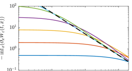
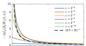
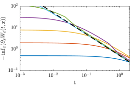
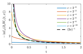
Figure 1. Illustration of $-\inf\partial_{x}W_{\varepsilon}$. Simulations for the initial datum $\rho_{0}:=\frac{1}{2}\mathds{1}_{(-0.5,0.5)}$ and velocity $V(\xi)=1-\xi$. Top row: kernel $\eta(\cdot):=\varepsilon^{-1}\exp(-\cdot\varepsilon^{-1})$. Bottom row: kernel $\eta:=\varepsilon^{-1}\mathds{1}_{(0,\varepsilon)}$.

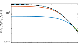
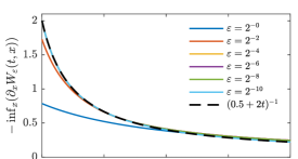
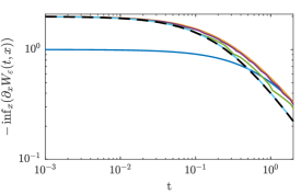
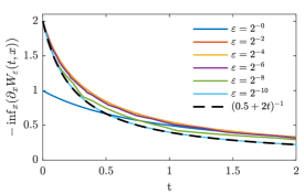
Figure 2. Illustration of $-\inf_{x\in\mathbb{R}}\partial_{x}W_{\varepsilon}(t,x)$. Simulations for the initial datum $\rho_{0}(\cdot):=(1-2|\cdot|)\mathds{1}_{(-0.5,0.5)}$ and velocity $V(\xi)=1-\xi$. Top row: kernel $\eta(\cdot):=\varepsilon^{-1}\exp(-\cdot\varepsilon^{-1})$. Bottom row: kernel $\eta(\cdot):=\varepsilon^{-1}\mathds{1}_{(0,\varepsilon)}(\cdot)$

.

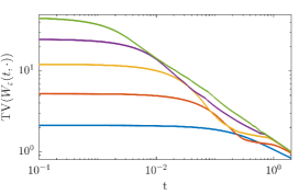
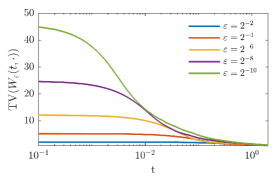
Figure 3. Illustration of $\mathrm{TV}(W_{\varepsilon}(t,\cdot))$. Total variations of the nonlocal term $W_{\varepsilon}$ for an initial datum with unbounded total variation, i.e., $\rho_{0}\>=\sum_{n=1}^{\infty}\mathds{1}_{(1/{n+1},1/n+1+1/(2n(n+1)))}$, linear velocity $V(\xi)=1-\xi$, and exponential kernel, i.e., $\eta(\cdot):=\varepsilon^{-1}\exp(-\cdot\varepsilon^{-1})$.

6. Open problems

In this contribution, we proved several Oleĭnik-type inequalities for nonlocal conservation laws with exponential kernel. As a byproduct, we obtained some convergence results for the nonlocal-to-local limit problem without monotonicity or total variation assumptions on the initial data. Several questions remain open for future work:

1. the case of more general velocity functions (which, in turn, means more general initial data) that do not satisfy the technical assumptions in Theorems 2.1 or 2.3;

2. the case of more general nonlocal weights (i.e., not necessarily of exponential type), as considered in [15].

References

• [1] F. Ancona, O. Glass, and K. T. Nguyen. Lower compactness estimates for scalar balance laws. Comm. Pure Appl. Math., 65(9):1303–1329, 2012.
• [2] S. Blandin and P. Goatin. Well-posedness of a conservation law with non-local flux arising in traffic flow modeling. Numer. Math., 132(2):217–241, 2016.
• [3] F. Bouchut and F. James. One-dimensional transport equations with discontinuous coefficients. Nonlinear Anal., 32(7):891–933, 1998.
• [4] F. Bouchut, F. James, and S. Mancini. Uniqueness and weak stability for multi-dimensional transport equations with one-sided Lipschitz coefficient. Ann. Sc. Norm. Super. Pisa Cl. Sci. (5), 4(1):1–25, 2005.
• [5] A. Bressan and R. M. Colombo. Decay of positive waves in nonlinear systems of conservation laws. Ann. Scuola Norm. Sup. Pisa Cl. Sci. (4), 26(1):133–160, 1998.
• [6] A. Bressan and W. Shen. On traffic flow with nonlocal flux: a relaxation representation. Arch. Ration. Mech. Anal., 237(3):1213–1236, 2020.
• [7] A. Bressan and W. Shen. Entropy admissibility of the limit solution for a nonlocal model of traffic flow. Commun. Math. Sci., 19(5):1447–1450, 2021.
• [8] K. S. Cheng. A regularity theorem for a nonconvex scalar conservation law. J. Differential Equations, 61(1):79–127, 1986.
• [9] G. M. Coclite, J.-M. Coron, N. De Nitti, A. Keimer, and L. Pflug. A general result on the approximation of local conservation laws by nonlocal conservation laws: The singular limit problem for exponential kernels. Ann. Inst. H. Poincaré Anal. Non Linéaire, 2022.
• [10] G. M. Coclite, N. De Nitti, A. Keimer, and L. Pflug. Singular limits with vanishing viscosity for nonlocal conservation laws. Nonlinear Analysis, 211:Paper No. 112370, 12, 2021.
• [11] G. M. Coclite, N. De Nitti, A. Keimer, and L. Pflug. On existence and uniqueness of weak solutions to nonlocal conservation laws with BV kernels. Z. Angew. Math. Phys., 73(6):Paper No. 241, 2022.
• [12] G. M. Coclite, N. De Nitti, A. Keimer, L. Pflug, and E. Zuazua. Long-time convergence of a nonlocal Burgers’ equation towards the local N-wave. Submitted, 2023.
• [13] M. Colombo, G. Crippa, M. Graff, and L. V. Spinolo. On the role of numerical viscosity in the study of the local limit of nonlocal conservation laws. ESAIM Math. Model. Numer. Anal., 55(6):2705–2723, 2021.
• [14] M. Colombo, G. Crippa, E. Marconi, and L. V. Spinolo. Local limit of nonlocal traffic models: convergence results and total variation blow-up. Ann. Inst. H. Poincaré C Anal. Non Linéaire, 38(5):1653–1666, 2021.
• [15] M. Colombo, G. Crippa, E. Marconi, and L. V. Spinolo. Nonlocal traffic models with general kernels: singular limit, entropy admissibility, and convergence rate. Arch. Ration. Mech. Anal., 247(2), 2023.
• [16] M. Colombo, G. Crippa, and L. V. Spinolo. On the singular local limit for conservation laws with nonlocal fluxes. Arch. Ration. Mech. Anal., 233(3):1131–1167, 2019.
• [17] J.-M. Coron, A. Keimer, and L. Pflug. Nonlocal transport equations—existence and uniqueness of solutions and relation to the corresponding conservation laws. SIAM J. Math. Anal., 52(6):5500–5532, 2020.
• [18] C. M. Dafermos. Characteristics in hyperbolic conservation laws. A study of the structure and the asymptotic behaviour of solutions. In Nonlinear analysis and mechanics: Heriot-Watt Symposium (Edinburgh, 1976), Vol. I, Res. Notes in Math., No. 17, pages 1–58. Pitman, London, 1977.
• [19] C. M. Dafermos. Hyperbolic conservation laws in continuum physics, volume 325 of Grundlehren der Mathematischen Wissenschaften [Fundamental Principles of Mathematical Sciences]. Springer-Verlag, Berlin, fourth edition, 2016.
• [20] C. De Lellis and F. Golse. A quantitative compactness estimate for scalar conservation laws. Comm. Pure Appl. Math., 58(7):989–998, 2005.
• [21] M. Garavello and B. Piccoli. Traffic flow on networks. Conservation laws models, volume 1 of AIMS Series on Applied Mathematics. American Institute of Mathematical Sciences (AIMS), Springfield, MO, 2006.
• [22] F. Ghiraldin and X. Lamy. Optimal Besov differentiability for entropy solutions of the eikonal equation. Comm. Pure Appl. Math., 73(2):317–349, 2020.
• [23] O. Glass. An extension of Oleinik’s inequality for general 1D scalar conservation laws. J. Hyperbolic Differ. Equ., 5(1):113–165, 2008.
• [24] P. Goatin and S. Scialanga. Well-posedness and finite volume approximations of the LWR traffic flow model with non-local velocity. Netw. Heterog. Media, 11(1):107–121, 2016.
• [25] D. Hoff. The sharp form of Oleĭnik’s entropy condition in several space variables. Trans. Amer. Math. Soc., 276(2):707–714, 1983.
• [26] E. Hopf. The partial differential equation $u_{t}+uu_{x}=\mu u_{xx}$. Comm. Pure Appl. Math., 3:201–230, 1950.
• [27] H. K. Jenssen and C. Sinestrari. On the spreading of characteristics for non-convex conservation laws. Proc. Roy. Soc. Edinburgh Sect. A, 131(4):909–925, 2001.
• [28] A. Keimer and L. Pflug. Existence, uniqueness and regularity results on nonlocal balance laws. J. Differential Equations, 263(7):4023–4069, 2017.
• [29] A. Keimer and L. Pflug. On approximation of local conservation laws by nonlocal conservation laws. J. Math. Anal. Appl., 475(2):1927–1955, 2019.
• [30] A. Keimer, L. Pflug, and M. Spinola. Existence, uniqueness and regularity of multi-dimensional nonlocal balance laws with damping. J. Math. Anal. Appl., 466(1):18–55, 2018.
• [31] A. Keimer, L. Pflug, and M. Spinola. Nonlocal scalar conservation laws on bounded domains and applications in traffic flow. SIAM J. Math. Anal., 50(6):6271–6306, 2018.
• [32] A. Keimer, L. Pflug, and M. Spinola. Nonlocal balance laws: Theory of convergence for nondissipative numerical schemes. Submitted, 2020.
• [33] O. A. Ladyženskaya. On the construction of discontinuous solutions of quasi-linear hyperbolic equations as limits of solutions of the corresponding parabolic equations when the “coefficient of viscosity” tends toward zero. Trudy Moskov. Mat. Obšč., 6:465–480, 1957.
• [34] P. D. Lax. Weak solutions of nonlinear hyperbolic equations and their numerical computation. Comm. Pure Appl. Math., 7:159–193, 1954.
• [35] P. D. Lax. Hyperbolic systems of conservation laws. II. Comm. Pure Appl. Math., 10:537–566, 1957.
• [36] P. G. LeFloch and K. Trivisa. Continuous Glimm-type functionals and spreading of rarefaction waves. Commun. Math. Sci., 2(2):213–236, 2004.
• [37] E. Marconi. The rectifiability of the entropy defect measure for Burgers equation. J. Funct. Anal., 283(6):Paper No. 109568, 19, 2022.
• [38] O. A. Oleĭnik. Discontinuous solutions of non-linear differential equations. Amer. Math. Soc. Transl. (2), 26:95–172, 1963.
• [39] L. Tartar. Compensated compactness and applications to partial differential equations. In Nonlinear analysis and mechanics: Heriot-Watt Symposium, Vol. IV, volume 39 of Res. Notes in Math., pages 136–212. Pitman, Boston, Mass.-London, 1979.