Sparse Cholesky Factorization for Solving Nonlinear PDEs via Gaussian Processes

Abstract

We study the computational scalability of a Gaussian process (GP) framework for solving general nonlinear partial differential equations (PDEs). This framework transforms solving PDEs to solving quadratic optimization problem with nonlinear constraints. Its complexity bottleneck lies in computing with dense kernel matrices obtained from pointwise evaluations of the covariance kernel of the GP and its partial derivatives at collocation points.

We present a sparse Cholesky factorization algorithm for such kernel matrices based on the near-sparsity of the Cholesky factor under a new ordering of Diracs and derivative measurements. We rigorously identify the sparsity pattern and quantify the exponentially convergent accuracy of the corresponding Vecchia approximation of the GP, which is optimal in the Kullback-Leibler divergence. This enables us to compute $\epsilon$-approximate inverse Cholesky factors of the kernel matrices with complexity $O(N\log^{d}(N/\epsilon))$ in space and $O(N\log^{2d}(N/\epsilon))$ in time.

With the sparse factors, gradient-based optimization methods become scalable. Furthermore, we can use the oftentimes more efficient Gauss-Newton method, for which we apply the conjugate gradient algorithm with the sparse factor of a reduced kernel matrix as a preconditioner to solve the linear system. We numerically illustrate our algorithm’s near-linear space/time complexity for a broad class of nonlinear PDEs such as the nonlinear elliptic, Burgers, and Monge-Ampère equations. In summary, we provide a fast, scalable, and accurate method for solving general PDEs with GPs.

65F30, 60G15, 65N75, 65M75, 65F50, 68W40

1 Introduction

Machine learning and probabilistic inference [43] have become increasingly popular due to their ability to automate the solution of computational problems. Gaussian processes (GPs) [71] are a promising approach for combining the theoretical rigor of traditional numerical algorithms with the flexible design of machine learning solvers [47, 48, 54, 11, 7]. They also have deep connections to kernel methods [63, 60], neural networks [45, 33, 26], and meshless methods [60, 77]. This paper studies the computational efficiency of GPs in solving nonlinear PDEs, where we need to deal with dense kernel matrices with entries obtained from pointwise values and derivatives of the covariance kernel function of the GP. The methodology developed here may also be applied to other context where derivative information of a GP or function is available, such as in Bayes optimization [74].

1.1 The problem

The GP method in [7] transforms every nonlinear PDE into the following quadratic optimization problem with nonlinear constraints:

(1) $$\left\{\begin{aligned} &\min_{\mathbf{z}\in\mathbb{R}^{N}}&&\mathbf{z}^{T}K({\bm{\phi}},{\bm{\phi}})^{-1}\mathbf{z}\\ &\mathrm{s.t.}&&{F(\mathbf{z})}={\mathbf{y}}\,,\end{aligned}\right.$$

where $F$ and $\mathbf{y}$ encode the PDE and source/boundary data. $K({\bm{\phi}},{\bm{\phi}})\in\mathbb{R}^{N\times N}$ is a positive definite kernel matrix whose entries are $k(\mathbf{x}_{i},\mathbf{x}_{j})$ or (a linear combination of) derivatives of the kernel function such as $\Delta_{\mathbf{x}}k(\mathbf{x}_{i},\mathbf{x}_{j})$. Here $\mathbf{x}_{i},\mathbf{x}_{j}\in\mathbb{R}^{d}$ are some sampled collocation points in space. Entries like $k(\mathbf{x}_{i},\mathbf{x}_{j})$ arise from Diracs measurements while entries like $\Delta_{\mathbf{x}}k(\mathbf{x}_{i},\mathbf{x}_{j})$ come from derivative measurements of the GP. For more details of the methodology, see Section 2. Computing with the dense matrix $K({\bm{\phi}},{\bm{\phi}})$ naïvely results in $O(N^{3})$ space/time complexity.

1.2 Contributions

This paper presents an algorithm that runs with complexity $O(N\log^{d}(N/\epsilon))$ in space and $O(N\log^{2d}(N/\epsilon))$ in time, which outputs a permutation matrix $P_{\rm perm}$ and a sparse upper triangular matrix $U$ with $O(N\log^{d}(N/\epsilon))$ nonzero entries, such that

(2) $$\|K({\bm{\phi}},{\bm{\phi}})^{-1}-P_{\rm perm}^{T}U{U}^{T}P_{\rm perm}\|_{\mathrm{Fro}}\leq\epsilon\,,$$

where $\|\cdot\|_{\mathrm{Fro}}$ is the Frobenius norm. We elaborate the algorithm in Section 3.

Our error analysis, presented in Section 4, requires sufficient Diracs measurements to appear in the domain. The setting of the rigorous result is for a class of kernel functions that are Green functions of differential operators such as the Matérn-like kernels, although the algorithm is generally applicable. The analysis is based on the interplay between linear algebra, Gaussian process conditioning, screening effects, and numerical homogenization, which shows the exponential decay/near-sparsity of the inverse Cholesky factor of the kernel matrix after permutation.

To solve (1), one efficient method is to linearize the constraint and solve a sequential quadratic programming problem. This leads to a linear system that involves a reduced kernel matrix $K({\bm{\phi}}^{k},{\bm{\phi}}^{k}):=DF(\mathbf{z}^{k})K({\bm{\phi}},{\bm{\phi}})(DF(\mathbf{z}^{k}))^{T}$ at each iterate $\mathbf{z}^{k}$; see Section 5. For this reduced kernel matrix, there are insufficient Diracs measurements in the domain, and we no longer have the above theoretical guarantee for its sparse Cholesky factorization. Nevertheless, we can still apply the algorithm with a slightly different permutation and couple it with preconditioned conjugate gradient (pCG) methods to solve the linear system. Our experiments demonstrate that nearly constant steps of pCG suffice for convergence.

For many nonlinear PDEs, we observe that the above sequential quadratic programming approach converges in $O(1)$ steps. Consequently, our algorithm leads to a near-linear space/time complexity solver for general nonlinear PDEs, assuming it converges. The assumption of convergence depends on the selection of kernels and the property of the PDE, and we demonstrate it numerically in solving nonlinear elliptic, Burgers, and Monge-Ampère equations; see Section 6.

1.3 Related work

1.3.1 Machine learning PDEs

Machine learning methods, such as those based on neural networks (NNs) and GPs, have shown remarkable promise in automating scientific computing, for instance in solving PDEs. Recent developments in this field include operator learning using prepared solution data [35, 5, 46, 38] and learning a single solution without any solution data [24, 55, 7, 27]. This paper focuses on the latter. NNs provide an expressive function representation. Empirical success has been widely reported in the literature. However, the training of NNs often requires significant tuning and takes much longer than traditional solvers [18]. Considerable research efforts have been devoted to stabilizing and accelerating the training process [31, 67, 68, 13, 76].

GP and kernel methods are based on a more interpretable and theoretically grounded function representation rooted in the Reproducing Kernel Hilbert Space (RKHS) theory [69, 3, 49]; with hierarchical kernel learning [73, 50, 10, 12], these representations can be made expressive as well. Nevertheless, working with dense kernel matrices is common, which often limits scalability. In the case of PDE problems, these matrices may also involve partial derivatives of the kernels [7], and fast algorithms for such matrices are less developed compared to the derivative-free counterparts.

1.3.2 Fast solvers for kernel matrices

Approximating dense kernel matrices (denoted by $\Theta$) is a classical problem in scientific computing and machine learning. Most existing methods focus on the case where $\Theta$ only involves the pointwise values of the kernel function. These algorithms typically rely on low-rank or sparse approximations, as well as their combination and multiscale variants. Low-rank techniques include Nyström’s approximations [70, 44, 6], rank-revealing Cholesky factorizations [19], inducing points via a probabilistic view [52], and random features [53]. Sparsity-based methods include covariance tapering [16], local experts (see a review in [37]), and approaches based on precision matrices and stochastic differential equations [36, 56, 59, 58]. Combining low-rank and sparse techniques can lead to efficient structured approximation [72] and can better capture short and long-range interactions [57]. Multiscale and hierarchical ideas have also been applied to seek for a full-scale approximation of $\Theta$ with a near-linear complexity. They include $\mathcal{H}$ matrix [21, 23, 22] and variants [34, 1, 2, 32, 42] that rely on the low-rank structure of the off-diagonal block matrices at different scales; wavelets-based methods [4, 17] that use the sparsity of $\Theta$ in the wavelet basis; multiresolution predictive processes [28]; and Vecchia approximations [66, 29] and sparse Cholesky factorizations [62, 61] that rely on the approximately sparse correlation conditioned on carefully ordered points.

For $\Theta$ that contains derivatives of the kernel function, several work [15, 51, 14] has utilized structured approximation to scale up the computation; no rigorous accuracy guarantee is proved. The inducing points approach [75, 41] has also been explored; however since this method only employs a low-rank approximation, the accuracy and efficiency can be limited.

1.3.3 Screening effects in spatial statistics

Notably, the sparse Cholesky factorization algorithm in [61], formally equivalent to Vecchia’s approximation [66, 29], achieves a state-of-the-art complexity $O(N\log^{d}(N/\epsilon))$ in space and $O(N\log^{2d}(N/\epsilon))$ in time for a wide range of kernel functions, with a rigorous theoretical guarantee. This algorithm is designed for kernel matrices with derivative-free entries and is connected to the screening effect in spatial statistics [64, 65]. The screening effect implies that approximate conditional independence of a spatial random field is likely to occur, under suitable ordering of points. The line of work [48, 49, 62] provides quantitative exponential decay results for the conditional covariance in the setting of a coarse-to-fine ordering of data points, laying down the theoretical groundwork for [61].

A fundamental question is how the screening effect behaves when derivative information of the spatial field is incorporated, and how to utilize it to extend sparse Cholesky factorization methods to kernel matrices that contain derivatives of the kernel. The screening effect studied within this new context can be useful for numerous applications where derivative-type measurements are available.

2 Solving nonlinear PDEs via GPs

In this section, we review the GP framework in [7] for solving nonlinear PDEs. We will use a prototypical nonlinear elliptic equation as our running example to demonstrate the main ideas, followed by more complete recipes for general nonlinear PDEs.

Consider the following nonlinear elliptic PDE:

(3) $$\left\{\begin{aligned} -\Delta u+\tau(u)&=f\quad\text{in }\Omega\,,\\ u&=g\quad\text{on }\partial\Omega\,,\end{aligned}\right.$$

where $\tau$ is a nonlinear scalar function and $\Omega$ is a bounded open domain in $\mathbb{R}^{d}$ with a Lipschitz boundary. We assume the equation has a strong solution in the classical sense.

2.1 The GP framework

The first step is to sample $M_{\Omega}$ collocation points in the interior and $M_{\partial\Omega}$ on the boundary such that

$$\mathbf{x}_{\Omega}=\{\mathbf{x}_{1},...,\mathbf{x}_{M_{\Omega}}\}\subset\Omega\quad\text{and}\quad\mathbf{x}_{\partial\Omega}=\{\mathbf{x}_{M_{\Omega}+1},...,\mathbf{x}_{M}\}\subset\partial\Omega\,,$$

where $M=M_{\Omega}+M_{\partial\Omega}$. Then, by assigning a GP prior to the unknown function $u$ with mean $0$ and covariance function $K:\overline{\Omega}\times\overline{\Omega}\to\mathbb{R}$, the method aims to compute the maximum a posterior (MAP) estimator of the GP given the sampled PDE data, which leads to the following optimization problem

(4) $$\left\{\begin{aligned} &\operatorname*{{\rm minimize}}_{u\in\mathcal{U}}~{}\|u\|&&\\ &{\rm\,s.t.}\quad-\Delta u(\mathbf{x}_{m})+\tau(u(\mathbf{x}_{m}))=f(\mathbf{x}_{m}),\quad&&\text{for }m=1,\ldots,M_{\Omega}\,,\\ &\hskip 25.83325ptu(\mathbf{x}_{m})=g(\mathbf{x}_{m}),\quad&&\text{for }m=M_{\Omega}+1,\ldots,M\,.\end{aligned}\right.$$

Here, $\|\cdot\|$ is the Reproducing Kernel Hilbert Space (RKHS) norm corresponding to the kernel/covariance function $K$.

Regarding consistency, once $K$ is sufficiently regular, the above solution will converge to the exact solution of the PDE when $M_{\Omega},M_{\partial\Omega}\to\infty$; see Theorem 1.2 in [7]. The methodology can be seen as a nonlinear generalization of many radial basis function based meshless methods [60] and probabilistic numerics [47, 11].

2.2 The finite dimensional problem

The next step is to transform (4) into a finite-dimensional problem for computation. We first introduce some notations:

• Notations for measurements: We denote the measurement functions by

  $$\phi^{(1)}_{m}=\updelta_{\mathbf{x}_{m}},1\leq m\leq M\quad\text{and}\quad\phi^{(2)}_{m}=\updelta_{\mathbf{x}_{m}}\circ\Delta,1\leq m\leq M_{\Omega}\,,$$

  where $\updelta_{\mathbf{x}}$ is the Dirac delta function centered at $\mathbf{x}$. They are in $\mathcal{U}^{*}$, the dual space of $\mathcal{U}$, for sufficiently regular kernel functions.

  Further, we use the shorthand notation ${\bm{\phi}}^{(1)}$ and ${\bm{\phi}}^{(2)}$ for the $M$ and $M_{\Omega}$-dimensional vectors with entries $\phi^{(1)}_{m}$ and $\phi^{(2)}_{m}$ respectively, and ${\bm{\phi}}$ for the $N$-dimensional vector obtained by concatenating ${\bm{\phi}}^{(1)}$ and ${\bm{\phi}}^{(2)}$, where $N=M+M_{\Omega}$.

• Notations for primal dual pairing: We use $[\cdot,\cdot]$ to denote the primal dual pairing, such that for $u\in\mathcal{U},\phi^{(1)}_{m}=\updelta_{\mathbf{x}_{m}}\in\mathcal{U}^{*}$, it holds that $[u,\phi^{(1)}_{m}]=u(\mathbf{x}_{m})$. Similarly $[u,\phi^{(2)}_{m}]=\Delta u(\mathbf{x}_{m})$ for $\phi^{(2)}_{m}=\updelta_{\mathbf{x}_{m}}\circ\Delta\in\mathcal{U}^{*}$. For simplicity of presentation, we oftentimes abuse the notation to write the primal-dual pairing in the $L^{2}$ integral form: $[u,\phi]=\int u(\mathbf{x})\phi(\mathbf{x})\,{\rm d}\mathbf{x}$.

• Notations for kernel matrices: We write $K({\bm{\phi}},{\bm{\phi}})$ as the $N\times N$-matrix with entries $\int K(\mathbf{x},\mathbf{x}^{\prime})\phi_{m}(\mathbf{x})\phi_{j}(\mathbf{x}^{\prime})\,{\rm d}\mathbf{x}\,{\rm d}\mathbf{x}^{\prime}$ where $\phi_{m}$ denotes the entries of ${\bm{\phi}}$. Here, the integral notation shall be interpreted as the primal-dual pairing as above.

  Similarly, $K(\mathbf{x},{\bm{\phi}})$ is the $N$ dimensional vector with entries $\int K(\mathbf{x},\mathbf{x}^{\prime})\phi_{j}(\mathbf{x}^{\prime})\,{\rm d}\mathbf{x}^{\prime}$. Moreover, we adopt the convention that if the variable inside a function is a set, it means that this function is applied to every element in this set; the output will be a vector or a matrix. As an example, $K(\mathbf{x}_{\Omega},\mathbf{x}_{\Omega})\in\mathbb{R}^{M_{\Omega}\times M_{\Omega}}$.

Then, based on a generalization of the representer theorem [7], the minimizer of (4) attains the form

$$u^{\dagger}(\mathbf{x})=K(\mathbf{x},{\bm{\phi}})K({\bm{\phi}},{\bm{\phi}})^{-1}\mathbf{z}^{\dagger}\,,$$

where $\mathbf{z}^{\dagger}$ is the solution to the following finite dimensional quadratic optimization problem with nonlinear constraints

(5) $$\left\{\begin{aligned} &\operatorname*{{\rm minimize}}_{\mathbf{z}\in\mathbb{R}^{M+M_{\Omega}}}\quad\mathbf{z}^{T}K({\bm{\phi}},{\bm{\phi}})^{-1}\mathbf{z}\\ &{\rm\,s.t.}\quad-z^{(2)}_{m}+\tau(z^{(1)}_{m})=f(\mathbf{x}_{m}),&&\text{for }m=1,\ldots,M_{\Omega}\,,\\ &\hskip 25.83325ptz^{(1)}_{m}=g(\mathbf{x}_{m}),&&\text{for }m=M_{\Omega}+1,\ldots,M\,.\end{aligned}\right.$$

Here, $\mathbf{z}^{(1)}\in\mathbb{R}^{M}$, $\mathbf{z}^{(2)}\in\mathbb{R}^{M_{\Omega}}$ and $\mathbf{z}$ is the concatenation of them. For this specific example, we can write down $K(\mathbf{x},{\bm{\phi}})$ and $K({\bm{\phi}},{\bm{\phi}})$ explicitly:

(6) $$K(\mathbf{x},{\bm{\phi}})=\left(K(\mathbf{x},\mathbf{x}_{\Omega}),K(\mathbf{x},\mathbf{x}_{\partial\Omega}),\Delta_{\mathbf{y}}K(\mathbf{x},\mathbf{x}_{\Omega})\right)\in\mathbb{R}^{1\times N}\,,$$

$$K({\bm{\phi}},{\bm{\phi}})=\begin{pmatrix}K(\mathbf{x}_{\Omega},\mathbf{x}_{\Omega})&K(\mathbf{x}_{\Omega},\mathbf{x}_{\partial\Omega})&\Delta_{\mathbf{y}}K(\mathbf{x}_{\Omega},\mathbf{x}_{\Omega})\\ K(\mathbf{x}_{\partial\Omega},\mathbf{x}_{\Omega})&K(\mathbf{x}_{\partial\Omega},\mathbf{x}_{\partial\Omega})&\Delta_{\mathbf{y}}K(\mathbf{x}_{\partial\Omega},\mathbf{x}_{\Omega})\\ \Delta_{\mathbf{x}}K(\mathbf{x}_{\Omega},\mathbf{x}_{\Omega})&\Delta_{\mathbf{x}}K(\mathbf{x}_{\Omega},\mathbf{x}_{\partial\Omega})&\Delta_{\mathbf{x}}\Delta_{\mathbf{y}}K(\mathbf{x}_{\Omega},\mathbf{x}_{\Omega})\end{pmatrix}\in\mathbb{R}^{N\times N}\,.$$

Here, $\Delta_{\mathbf{x}},\Delta_{\mathbf{y}}$ are the Laplacian operator for the first and second arguments of $k$, respectively. Clearly, evaluating the loss function and its gradient requires us to deal with the dense kernel matrix $K({\bm{\phi}},{\bm{\phi}})$ with entries comprising derivatives of $k$.

2.3 The general case

For general PDEs, the methodology leads to the optimization problem

$$\left\{\begin{aligned} &\min_{u\in\mathcal{U}}~{}&&\|u\|\\ &\mathrm{s.t.}&&\text{PDE constraints at $\{\mathbf{x}_{1},\dots,\mathbf{x}_{M}\}\in\overline{\Omega}$}\,,\end{aligned}\right.$$

and the equivalent finite dimensional problem

(7) $$\left\{\begin{aligned} &\min_{\mathbf{z}\in\mathbb{R}^{N}}&&\mathbf{z}^{T}K({\bm{\phi}},{\bm{\phi}})^{-1}\mathbf{z}\\ &\mathrm{s.t.}&&{F(\mathbf{z})}={\mathbf{y}}\,,\end{aligned}\right.$$

where ${\bm{\phi}}$ is the concatenation of Diracs measurements and derivative measurements of $u$; they are induced by the PDE at the sampled points. The function $F$ encodes the PDE, and the vector $\mathbf{y}$ encodes the right hand side and boundary data. Again, it is clear that the computational bottleneck lies in the part $K({\bm{\phi}},{\bm{\phi}})^{-1}$.

Here, we use “derivative measurement” to mean a functional in $\mathcal{U}^{*}$ whose action on a function in $\mathcal{U}$ leads to a linear combination of its derivatives. Mathematically, suppose the highest order of derivatives is $J$, then the corresponding derivative measurement at point $\mathbf{x}_{m}$ can be written as $\phi=\sum_{|\gamma|\leq J}{a_{\gamma}}\updelta_{\mathbf{x}_{m}}\circ D^{\gamma}$ with the multi-index $\gamma=(\gamma_{1},...,\gamma_{d})\in\mathbb{N}^{d}$ and $|\gamma|:=\sum_{k=1}^{d}\gamma_{k}\leq J$. Here $D^{\gamma}:=D^{\gamma_{1}}_{\mathbf{x}^{(1)}}\cdots D^{\gamma_{d}}_{\mathbf{x}^{(d)}}$ is a $|\gamma|$-th order differential operator, and we use the notation $\mathbf{x}=(\mathbf{x}^{(1)},...,\mathbf{x}^{(d)})$. We require linear independence between these measurements to ensure $K({\bm{\phi}},{\bm{\phi}})$ is invertible.

3 The sparse Cholesky factorization algorithm

In this section, we present a sparse Cholesky factorization algorithm for $K({\bm{\phi}},{\bm{\phi}})^{-1}$. Theoretical results will be presented in Section 4 based on the interplay between linear algebra, Gaussian process conditioning, screening effects in spatial statistics, and numerical homogenization.

In Subsection 3.1, we summarize the state-of-the-art sparse Cholesky factorization algorithm for kernel matrices with derivative-free measurements. In Subsection 3.2, we discuss an extension of the idea to kernel matrices with derivative-type measurements, which are the main focus of this paper. The algorithm presented in Subsection 3.2 leads to near-linear complexity evaluation of the loss function and its gradient in the GP method for solving PDEs. First-order methods thus become scalable. We then extend the algorithm to second-order optimization methods (e.g., the Gauss-Newton method) in Section 5.

3.1 The case of derivative-free measurements

We start the discussion with the case where ${\bm{\phi}}$ contains Diracs-type measurements only.

Consider a set of points $\{\mathbf{x}_{i}\}_{i\in I}\subset\Omega$, where $I=\{1,2,...,M\}$ as in Subsection 2.1. We assume the points are scattered; to quantify this, we have the following definition of homogeneity:

Definition 3.1.

The homogeneity parameter of the points $\{\mathbf{x}_{i}\}_{i\in I}\subset\Omega$ conditioned on a set $\mathsf{A}$ is defined as

$$\delta(\{\mathbf{x}_{i}\}_{i\in I};\mathsf{A})=\frac{\min_{\mathbf{x}_{i},\mathbf{x}_{j}\in I}\mathrm{dist}(\mathbf{x}_{i},\{\mathbf{x}_{j}\}\cup\mathsf{A})}{\max_{\mathbf{x}\in\Omega}\mathrm{dist}(\mathbf{x},\{\mathbf{x}_{i}\}_{i\in I}\cup\mathsf{A})}\,.$$

When $\mathsf{A}=\emptyset$, we also write $\delta(\{\mathbf{x}_{i}\}_{i\in I}):=\delta(\{\mathbf{x}_{i}\}_{i\in I};\emptyset)$.

Throughout this paper, we assume $\delta(\{\mathbf{x}_{i}\}_{i\in I})>0$. One can understand that a larger $\delta(\{\mathbf{x}_{i}\}_{i\in I})$ makes the distribution of points more homogeneous in space. It can also be useful to consider $\mathsf{A}=\partial\Omega$ if one wants the points not too close to the boundary.

Let ${\bm{\phi}}$ be the collection of $\updelta_{\mathbf{x}_{i}},1\leq i\leq M$; all of them are Diracs-type measurements and thus derivative-free. In [61], a sparse Choleksy factorization algorithm was proposed to factorize $K({\bm{\phi}},{\bm{\phi}})^{-1}$. We summarize this algorithm (with a slight modification) in the following three steps: reordering, sparsity pattern, and Kullback-Leibler (KL) minimization.

3.1.1 Reordering

The first step is to reorder these points from coarse to fine scales. It can be achieved by the maximum-minimum distance ordering (maximin ordering) [20]. We define a generalization to conditioned maximin ordering as follows:

Definition 3.2 (Conditioned Maximin Ordering).

The maximin ordering conditioned on a set $\mathsf{A}$ for points $\{\mathbf{x}_{i},i\in I\}$ is obtained by successively selecting the point $\mathbf{x}_{i}$ that is furthest away from $\mathsf{A}$ and the already picked points. If $\mathsf{A}$ is an empty set, then we select an arbitrary index $i\in I$ as the first to start. Otherwise, we choose the first index as

$$i_{1}={\arg\max}_{i\in I}\operatorname{dist}(\mathbf{x}_{i},\mathsf{A})\,.$$

For the first $q$ indices already chosen, we choose

$$i_{q+1}={\arg\max}_{i\in I\backslash\{i_{1},...,i_{q}\}}\operatorname{dist}(\mathbf{x}_{i},\{\mathbf{x}_{i_{1}},...,\mathbf{x}_{i_{q}}\}\cup\mathsf{A})\,.$$

Usually we set $\mathsf{A}=\partial\Omega$ or $\emptyset$. We introduce the operator $P:I\to I$ to map the order of the measurements to the index of the corresponding points, i.e., $P(q)=i_{q}$. One can define the lengthscale of each ordered point as

(8) $$l_{i}=\mathrm{dist}(\mathbf{x}_{P(i)},\{\mathbf{x}_{P(1)},...,\mathbf{x}_{P(i-1)}\}\cup\mathsf{A})\,.$$

Let $\Theta=K(\tilde{{\bm{\phi}}},\tilde{{\bm{\phi}}})\in\mathbb{R}^{N\times N}$ be the kernel matrix after reordering the measurements in ${\bm{\phi}}$ to $\tilde{{\bm{\phi}}}=(\phi_{P(1)},...,\phi_{P(M)})$; we have $N=M$ in this setting. An important observation is that the Cholesky factors of $\Theta$ and $\Theta^{-1}$ could exhibit near-sparsity under the maximin ordering. Indeed, as an example, suppose $\Theta^{-1}=U^{\star}{U^{\star}}^{T}$ where $U^{\star}$ is the upper Cholesky factor. Then in Figure 1, we show the magnitude of $U^{\star}_{ij},i\leq j$ for a Matérn kernel, where $j=1000,2000$; the total number of points is $M=51^{2}$. It is clear from the figure that the entries decay very fast when the points move far away from the current $j$th ordered point.

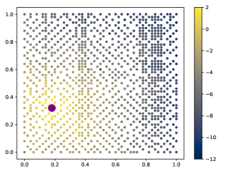
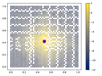
Figure 1: Demonstration of screening effects in the context of Diracs measurements using the Matérn kernel with $\nu=5/2$ and lengthscale $0.3$. The data points are equidistributed in $[0,1]^{2}$ with grid size $h=0.02$. In the left figure, we display the $1000$th point (the big point) in the maximin ordering with $\mathsf{A}=\emptyset$, where all points ordered before it (i.e., $i<1000$) are colored with intensity according to the corresponding $|U_{ij}^{\star}|$. The right figure is generated in the same manner but for the $2000$th point in the ordering.

One may wonder why such a coarse-to-fine reordering leads to sparse Cholesky factors. In fact, we can interpret entries of $U^{\star}$ as the conditional covariance of some GP. More precisely, consider the GP $\xi\sim\mathcal{GP}(0,K)$. Then, by definition, the Gaussian random variables $Y_{i}:=[\xi,\tilde{\phi}_{i}]\sim\mathcal{N}(0,K(\tilde{\phi}_{i},\tilde{\phi}_{i}))$. We have the following relation:

(9) $$\frac{U^{\star}_{ij}}{U^{\star}_{jj}}=(-1)^{i\neq j}\frac{\mathrm{Cov}[Y_{i},Y_{j}|Y_{1:j-1\backslash\{i\}}]}{\mathrm{Var}[Y_{i}|Y_{1:j-1\backslash\{i\}}]},\quad i\leq j\,.$$

Here we used the MATLAB notation such that $Y_{1:j-1\backslash\{i\}}$ corresponds to $\{Y_{q}:1\leq q\leq j-1,q\neq i\}$. Proof of this formula can be found in Appendix D.3.

Formula (9) links the values of $U^{\star}$ to the conditional covariance of a GP. In spatial statistics, it is well-known from empirical evidence that conditioning a GP on coarse-scale measurements results in very small covariance values between finer-scale measurements. This phenomenon, known as screening effects, has been discussed in works such as [64, 65]. The implication is that conditioning on coarse scales screens out fine-scale interactions.

As a result, one would expect the corresponding Cholesky factor to become sparse upon reordering. Indeed, the off-diagonal entries exhibit exponential decay. A rigorous proof of the quantitative decay can be found in [62], where the measurements consist of Diracs functionals only, and the kernel function is the Green function of some differential operator subject to Dirichlet boundary conditions. The proof of Theorem 6.1 in [62] effectively implies that

(10) $$|U^{\star}_{ij}|\leq C_{1}l_{M}^{C_{2}}\exp\left(-\frac{\operatorname{dist}(\mathbf{x}_{P(i)},\mathbf{x}_{P(j)})}{C_{1}l_{j}}\right)$$

for some generic constants $C_{1},C_{2}$ depending on the domain, kernel function, and homogeneity parameter of the points. We will prove such decay also holds when derivative-type measurements are included, in Section 4 under a novel ordering. It is worth mentioning that our analysis also provides a much simpler proof for (10).

3.1.2 Sparsity pattern

With the ordering determined, our next step is to identify the sparsity pattern of the Cholesky factor under the ordering.

For a tuning parameter $\rho\in\mathbb{R}^{+}$, we select the upper-triangular sparsity set $S_{P,l,\rho}\subset I\times I$ as

(11) $$S_{P,l,\rho}=\{(i,j)\subset I\times I:i\leq j,\,\operatorname{dist}(\mathbf{x}_{P(i)},\mathbf{x}_{P(j)})\leq\rho l_{j}\}\,.$$

The choice of the sparsity pattern is motivated by the quantitative exponential decay result mentioned in Remark LABEL:remark:_why_coarse-to-fine_ordering. Here in the subscript, $P$ stands for the ordering, $l$ is the lengthscale parameter associated with the ordering, and $\rho$ is a hyperparameter that controls the size of the sparsity pattern. We sometimes drop the subscript to simplify the notation when there is no confusion. We note that the cardinality of the set $S_{P,l,\rho}$ is bounded by $O(N\rho^{d})$, through a ball-packing argument (see Appendix B).

The maximin ordering and the sparsity pattern can be constructed with computational complexity $O(N\log^{2}(N)\rho^{d})$ in time and $O(N\rho^{d})$ in space; see Algorithm 4.1 and Theorem 4.1 in [61].

3.1.3 KL minimization

With the ordering and sparsity pattern identified, the last step is to use KL minimization to compute the best approximate sparse Cholesky factors given the pattern.

Define the set of sparse upper-triangular matrices with sparsity pattern $S_{P,l,\rho}$ as

(12) $$\mathcal{S}_{P,l,\rho}:=\{A\in\mathbb{R}^{N\times N}:A_{ij}\neq 0\Rightarrow(i,j)\in S_{P,l,\rho}\}\,.$$

For each column $j$, denote $s_{j}=\{i:(i,j)\in S_{P,l,\rho}\}$. The cardinality of the set $s_{j}$ is denoted by $\#s_{j}$.

The KL minimization step seeks to find

(13) $$U={\arg\min}_{\hat{U}\in\mathcal{S}_{P,l,\rho}}\operatorname{KL}\left(\mathcal{N}(0,\Theta)\parallel\mathcal{N}(0,(\hat{U}\hat{U}^{T})^{-1})\right)\,.$$

It turns out that the above problem has an explicit solution

(14) $$U_{s_{j},j}=\frac{\Theta_{s_{j},s_{j}}^{-1}\textbf{e}_{\#s_{j}}}{\sqrt{\textbf{e}_{\#s_{j}}^{T}\Theta_{s_{j},s_{j}}^{-1}\textbf{e}_{\#s_{j}}}}\,,$$

where $\textbf{e}_{\#s_{j}}$ is a standard basis vector in $\mathbb{R}^{\#s_{j}}$ with the last entry being $1$ and other entries equal $0$. Here, $\Theta_{s_{j},s_{j}}^{-1}:=(\Theta_{s_{j},s_{j}})^{-1}$. The proof of this explicit formula follows a similar approach to that of Theorem 2.1 in [61], with the only difference being the use of upper Cholesky factors. A detailed proof is provided in Appendix C. It is worth noting that the optimal solution is equivalent to the Vecchia approximation used in spatial statistics; see discussions in [61].

With the KL minimization, we can find the best approximation measured in the KL divergence sense, given the sparsity pattern. The computation is embarrassingly parallel, noting that the formula (14) are independent for different columns.

or the algorithm described above, the computational complexity is upper-bounded by $O(\sum_{1\leq i\leq N}(\#s_{j})^{3})$ in time and $O(\#S+\max_{1\leq i\leq N}(\#s_{j})^{2})$ in space when using dense Cholesky factorization to invert $\Theta_{s_{j},s_{j}}$.

When using the sparsity pattern $S_{P,l,\rho}$, we can obtain $\#s_{j}=O(\rho^{d})$ and $\#S=O(N\rho^{d})$ via a ball-packing argument (see Appendix B). This yields a complexity of $O(N\rho^{3d})$ in time and $O(N\rho^{d})$ in space.

The concept of supernodes [61], which relies on an extra parameter $\lambda$, can be utilized to group the sparsity pattern of nearby measurements and create an aggregate sparsity pattern $S_{P,l,\rho,\lambda}$. This technique reduces computation redundancy and improves the arithmetic complexity of the KL minimization to $O(N\rho^{2d})$ in time (see Appendix A). In this paper, we consistently employ this approach. [61], it was shown in Theorem 3.4 that $\rho=O(\log(N/\epsilon))$ suffices to get an $\epsilon$-approximate factor for a large class of kernel matrices, so the complexity of the KL minimization is $O(N\log^{2d}(N/\epsilon))$ in time and $O(N\log^{d}(N/\epsilon))$ in space. Note that the ordering and aggregate sparsity pattern can be constructed in time complexity $O(N\log^{2}(N)\rho^{d})$ and space complexity $O(N\rho^{d})$; the complexity of this construction step is usually of a lower order compared to that of the KL minimization. Moreover, this step can be pre-computed.

3.2 The case of derivative measurements

The last subsection discusses the sparse Cholesky factorization algorithm for kernel matrices that are generated by derivative-free measurements. When using GPs to solve PDEs and inverse problems, ${\bm{\phi}}$ can contain derivative measurements, which are the main focus of this paper. This subsection aims to deal with such scenarios.

3.2.1 The nonlinear elliptic PDE case

To begin with, we will consider the example in Subsection 2.2, where we have Diracs measurements $\phi^{(1)}_{m}=\updelta_{\mathbf{x}_{m}}$ for $1\leq m\leq M$, and Laplacian-type measurements $\phi^{(2)}_{m}=\updelta_{\mathbf{x}_{m}}\circ\Delta$ for $1\leq m\leq M_{\Omega}$. Our objective is to extend the algorithm discussed in the previous subsection to include these derivative measurements.

An important question we must address is the ordering of these measurements. Specifically, should we consider the Diracs measurements before or after the derivative-type measurements? To explore this question, we conduct the following experiment. First, we order all derivative-type measurements, $\phi^{(2)}_{m}$ for $1\leq m\leq M_{\Omega}$, in an arbitrary manner. We then follow this ordering with any Diracs measurement, labeled $M_{\Omega}+1$ in the order. For this measurement, we plot the magnitude of the corresponding Cholesky factor of $\Theta^{-1}$, i.e., $|U^{\star}_{ij}|$ for $i\leq j$ and $j=M_{\Omega}+1$, similar to the approach taken in Figure 1. The results are shown in the left part of Figure 2.

Unfortunately, we do not observe an evident decay in the left of Figure 2. This may be due to the fact that, even when conditioned on the Laplacian-type measurements, the Diracs measurements can still exhibit long-range interactions with other measurements. This is because there are degrees of freedom of harmonic functions that are not captured by Laplacian-type measurements, and thus, the correlations may not be effectively screened out.

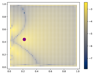
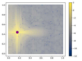
Figure 2: Demonstration of screening effects in the context of derivative-type measurements using the Matérn kernel with $\nu=5/2$ and lengthscale $0.3$. The data points are equidistributed in $[0,1]^{2}$ with grid size $h=0.02$. In the left figure, we order the Laplacian measurements first and then select a Diracs measurement which is the big point. The points are colored with intensity according to $|U_{ij}^{\star}|$. In the right figure, we order the Dircas measurements first and then select a Laplacian measurement; we display things in the same manner as the left figure.

Alternatively, we can order the Dirac measurements first and then examine the same quantity as described above for any Laplacian measurement. This approach yields the right part of Figure 2, where we observe a fast decay as desired. This indicates that the derivative measurements should come after the Dirac measurements, or equivalently, that the derivative measurements should be treated as finer scales compared to the pointwise measurements.

With the above observation, we can design our new ordering as follows. For the nonlinear elliptic PDE example in Subsection 2.2, we order the Diracs measurements $\phi^{(1)}_{m}=\updelta_{\mathbf{x}_{m}},1\leq m\leq M$ first using the maximin ordering with $\mathsf{A}=\emptyset$ mentioned earlier. Then, we add the derivative-type measurements $\updelta_{\mathbf{x}_{m}}\circ\Delta,1\leq m\leq M_{\Omega}$ in arbitrary order to the ordering.

Again, for our notations, we use $P:I_{N}\to I$ to map the index of the ordered measurements to the index of the corresponding points. Here $I_{N}:=\{1,2,...,N\}$, $N=M+M_{\Omega}$ and the cardinality of $I$ is $M$. We define the lengthscales of the ordered measurements to be

(15) $$l_{i}=\begin{cases}\mathrm{dist}(\mathbf{x}_{P(i)},\{\mathbf{x}_{P(1)},...,\mathbf{x}_{P(i-1)}\}\cup\mathsf{A}),&\text{if }i\leq M,\\ l_{M},&\text{otherwise.}\end{cases}$$

We will justify the above choice of lengthscales in our theoretical study in Section 4.

With the ordering and the lengthscales determined, we can apply the same steps in the last subsection to identify sparsity patterns:

(16) $$S_{P,l,\rho}=\{(i,j)\subset I_{N}\times I_{N}:i\leq j,\,\operatorname{dist}(\mathbf{x}_{P(i)},\mathbf{x}_{P(j)})\leq\rho l_{j}\}\subset I_{N}\times I_{N}\,.$$

Then, we can use KL minimization as in Subsection 3.1.3 (see (12), (13), and (14)) to find the optimal sparse factors under the pattern. This leads to our sparse Cholesky factorization algorithm for kernel matrices with derivative-type measurements.

Similar to Remark LABEL:rmk:_derivative-free_meas,_supernodes,_complexity, the above KL minimization step (with the idea of supernodes to aggregate the sparsity pattern) can be implemented in time complexity $O(N\rho^{2d})$ and space complexity $O(N\rho^{d})$, for a parameter $\rho\in\mathbb{R}^{+}$ that determines the size of the sparsity set.

We present some numerical experiments to demonstrate the accuracy of such an algorithm. In Figure 3, we show the error measured in the KL divergence sense, namely $\operatorname{KL}\left(\mathcal{N}(0,\Theta)\parallel\mathcal{N}(0,(U^{\rho}{U^{\rho}}^{T})^{-1})\right)$ where $U^{\rho}$ is the computed sparse factor. The figures show that the KL error decays exponentially fast regarding $\rho$. The rate is faster for less smooth kernels, and for the same kernel, the rate remains the same when there are more physical points. In the left of Figure 4, we show the CPU time of the algorithm, which scales nearly linearly regarding the number of points.

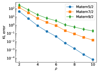
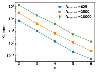
Figure 3: Demonstration of the accuracy of the sparse Cholesky factorization for $K({\bm{\phi}},{\bm{\phi}})^{-1}$ in the nonlinear elliptic PDE example. In the left figure, we choose Matérn kernels with $\nu=5/2,7/2,9/2$ and lengthscale $l=0.3$; the physical points are fixed to be equidistributed in $[0,1]^{2}$ with grid size $h=0.05$; we plot the error measured in the KL sense with regard to different $\rho$. In the right figure, we fix the Matérn kernels with $\nu=5/2$ and lengthscale $l=0.3$. We vary the number of physical points, which are equidistributed with grid size $h=0.04,0.02,0.01$; thus $N_{\rm domain}=625,2500,10000$ correspondingly.

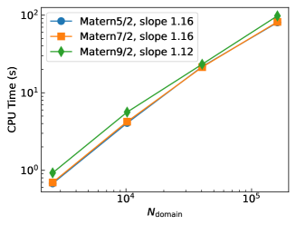
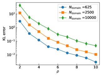
Figure 4: In the left figure, we choose Matérn kernels with $\nu=5/2,7/2,9/2$ and lengthscale $l=0.3$; the physical points are equidistributed in $[0,1]^{2}$ with different grid sizes; we plot the CPU time of the factorization algorithm for $K({\bm{\phi}},{\bm{\phi}})^{-1}$, using the personal computer MacBook Pro 2.4 GHz Quad-Core Intel Core i5. In the right figure, we study the sparse Cholesky factorization for the reduced kernel matrix $K({\bm{\phi}}^{k},{\bm{\phi}}^{k})^{-1}$. We fix the Matérn kernels with $\nu=5/2$ and lengthscale $l=0.3$. We vary the number of physical points, which are equidistributed with grid size $h=0.04,0.02,0.01$. We plot the KL error with regard to different $\rho$.

3.2.2 General case

We present the algorithm discussed in the last subsection for general PDEs. In the general case (7), we need to deal with $K({\bm{\phi}},{\bm{\phi}})$ where ${\bm{\phi}}$ is the concatenation of Diracs measurements and derivative-type measurements that are derived from the PDE. Suppose the number of physical points is $M$; they are $\{\mathbf{x}_{1},...,\mathbf{x}_{M}\}$ and the index set is denoted by $I=\{1,...,M\}$. Without loss of generality, we can assume ${\bm{\phi}}$ contains Diracs measurements $\updelta_{\mathbf{x}_{m}}$ at all these points and some derivative measurements at these points up to order $J\in\mathbb{N}$. See the definition of derivative measurements in Remark LABEL:remark:_def_of_derivative_measurements. The reason we can assume Diracs measurements are in ${\bm{\phi}}$ is that one can always add $0u(\mathbf{x})$ to the PDE if there are no terms involving $u(\mathbf{x})$. The presence of these Diracs measurements is the key to get provable guarantee of the algorithm; for details see Section 4.

Denote the total number of measurements by $N$, as before. We order the Diracs measurements $\updelta_{\mathbf{x}_{m}},1\leq m\leq M$ first using the maximin ordering with $\mathsf{A}=\emptyset$. Then, we add the derivative-type measurements in an arbitrary order to the ordering.

Similar to the last subsection, we use the notation $P:I_{N}\to I$ to map the index of the ordered measurements to the index of the corresponding points; here $I_{N}:=\{1,2,...,N\}$. The lengthscales of the ordered measurements are defined via (15). With the ordering, one can identify the sparsity pattern as in (16) (and aggregate it using supernodes as discussed in Remark LABEL:rmk:_derivative-free_meas,_supernodes,_complexity) and use the KL minimization (12)(13)(14) to compute $\epsilon$-approximate factors the same way as before. We outline the general algorithmic procedure in Algorithm 1.

Algorithm 1 Sparse Cholesky factorization for $K({\bm{\phi}},{\bm{\phi}})^{-1}$

Input: Measurements ${\bm{\phi}}$, kernel function $K$, sparsity parameter $\rho$, supernodes parameter $\lambda$
Output: $U^{\rho},P_{\rm perm}\ \mathrm{s.t.}\ K({\bm{\phi}},{\bm{\phi}})^{-1}\approx P_{\rm perm}^{T}U^{\rho}{U^{\rho}}^{T}P_{\rm perm}$

1:  Reordering and sparsity pattern: we first order the Diracs measurements using the maximin ordering. Next, we order the derivative measurements in an arbitrary order. This process yields a permutation matrix denoted by $P_{\rm perm}$, such that $P_{\rm perm}{\bm{\phi}}=\tilde{{\bm{\phi}}}$, and lengthscales $l$ for each measurement in $\tilde{{\bm{\phi}}}$. Under the ordering, we construct the aggregate sparsity pattern $S_{P,l,\rho,\lambda}$ based on the chosen values of $\rho$ and $\lambda$.

2:  KL minimization: solve (13) with $\Theta=K(\tilde{{\bm{\phi}}},\tilde{{\bm{\phi}}})$, by (14), to obtain $U^{\rho}$

3:  return  $U^{\rho},P_{\rm perm}$

The complexity is of the same order as in Remark LABEL:remark:_complexity_of_cholesky,_derivative_data,_nonlinear_elliptic_pde_eg; the hidden constant in the complexity estimate depends on $J$, the maximum order of the derivative measurements. We will present theoretical analysis for the approximation accuracy in Section 4, which implies that $\rho=O(\log(N/\epsilon))$ suffices to provide $\epsilon$-approximation for a large class of kernel matrices.

4 Theoretical study

In this section, we perform a theoretical study of the sparse Cholesky factorization algorithm in Subsection 3.2 for $K({\bm{\phi}},{\bm{\phi}})^{-1}$.

4.1 Set-up for rigorous results

We present the setting of kernels, physical points, and measurements for which we will provide rigorous analysis of the algorithm.

Kernel

We first describe the domains and the function spaces. Suppose $\Omega$ is a bounded convex domain in $\mathbb{R}^{d}$ with a Lipschitz boundary. Without loss of generality, we assume $\mathrm{diam}(\Omega)\leq 1$; otherwise, we can scale the domain. Let $H_{0}^{s}(\Omega)$ be the Sobolev space in $\Omega$ with order $s\in\mathbb{N}$ derivatives in $L^{2}$ and zero traces. Let the operator

$$\mathcal{L}:H^{s}_{0}(\Omega)\to H^{-s}(\Omega)$$

satisfy Assumption 1. This assumption is the same as in Section 2.2 of [49].

Assumption 1.

The following conditions hold for $\mathcal{L}:H^{s}_{0}(\Omega)\to H^{-s}(\Omega)$:

1. symmetry: $[u,\mathcal{L}v]=[v,\mathcal{L}u]$;

2. positive definiteness: $[u,\mathcal{L}u]>0$ for $\|u\|_{H^{s}_{0}(\Omega)}>0$;

3. boundedness:

   $$\|\mathcal{L}\|:=\sup_{u}\frac{\|\mathcal{L}u\|_{H^{-s}(\Omega)}}{\|u\|_{H^{s}_{0}(\Omega)}}<\infty,\quad\|\mathcal{L}^{-1}\|:=\sup_{u}\frac{\|\mathcal{L}^{-1}u\|_{H^{s}_{0}(\Omega)}}{\|u\|_{H^{-s}(\Omega)}}<\infty\,;$$

4. locality: $[u,\mathcal{L}v]=0$ if $u$ and $v$ have disjoint supports.

We assume $s>d/2$ so Sobolev’s embedding theorem shows that $H^{s}_{0}(\Omega)\subset C(\Omega)$, and thus $\updelta_{\mathbf{x}}\in H^{-s}(\Omega)$ for $\mathbf{x}\in\Omega$. We consider the kernel function to be the Green function $K(\mathbf{x},\mathbf{y}):=[\updelta_{\mathbf{x}},\mathcal{L}^{-1}\updelta_{\mathbf{y}}]$. An example of $\mathcal{L}$ could be $(-\Delta)^{s}$; we use the zero Dirichlet boundary condition to define $\mathcal{L}^{-1}$, which leads to a Matérn-like kernel.

Physical points

Consider a scattered set of points $\{\mathbf{x}_{i}\}_{i\in I}\subset\Omega$, where $I=\{1,2,...,M\}$ as in Subsection 3.1; the homogeneity parameter of these points is assumed to be positive:

$$\delta(\{\mathbf{x}_{i}\}_{i\in I};\partial\Omega)=\frac{\min_{\mathbf{x}_{i},\mathbf{x}_{j}\in I}\mathrm{dist}(\mathbf{x}_{i},\{\mathbf{x}_{j}\}\cup\partial\Omega)}{\max_{\mathbf{x}\in\Omega}\mathrm{dist}(\mathbf{x},\{\mathbf{x}_{i}\}_{i\in I}\cup\partial\Omega)}>0\,.$$

This condition ensures that the points are scattered homogeneously. Here we set $\mathsf{A}=\partial\Omega$ since we consider zero Dirichlet’s boundary condition and no points will be on the boundary. The accuracy in our theory will depend on $\delta(\{\mathbf{x}_{i}\}_{i\in I};\partial\Omega)$.

Measurements

The setting is the same as in Subsection 3.2.2. We assume ${\bm{\phi}}$ contains Diracs measurements at all of the scattered points, and it also contains derivative-type measurements at some of these points up to order $J\in\mathbb{N}$. We require $J<s-d/2$ so that the Sobolev embedding theorem guarantees these derivative measurements are well-defined.

For simplicity of analysis, we assume all the measurements are of the type $\updelta_{\mathbf{x}_{i}}\circ D^{\gamma}$ with the multi-index $\gamma=(\gamma_{1},...,\gamma_{d})\in\mathbb{N}^{d}$ and $|\gamma|:=\sum_{k=1}^{d}\gamma_{k}\leq J$; here $D^{\gamma}=D^{\gamma_{1}}_{\mathbf{x}^{(1)}}\cdots D^{\gamma_{d}}_{\mathbf{x}^{(d)}}$; see Remark LABEL:remark:_def_of_derivative_measurements. Note that when $|\gamma|=0$, $\updelta_{\mathbf{x}_{i}}\circ D^{\gamma}$ corresponds to Diracs measurements. The total number of measurements is denoted by $N$.

Note that the aforementioned assumption does not apply to the scenario of Laplacian measurements in the case of a nonlinear elliptic PDE example. This exclusion is solely for the purpose of proof convenience, as it necessitates linear independence of measurements. However, similar proofs can be applied to Laplacian measurements once linear independence between the measurements is ensured.

4.2 Theory

Under the setting in Subsection 4.1, we consider the ordering $P:\{1,2,...,N\}\to\{1,2,...,M\}$ described in Subsection 3.2.2. Recall that for this $P$, we first order the Diracs measurements using the maximin ordering conditioned on $\partial\Omega$ (since there are no boundary points); then, we follow the ordering with an arbitrary order of the derivative measurements. The lengthscale parameters are defined via

$$l_{i}=\begin{cases}\mathrm{dist}(\mathbf{x}_{P(i)},\{\mathbf{x}_{P(1)},...,\mathbf{x}_{P(i-1)}\}\cup\partial\Omega),&\text{if }i\leq M,\\ l_{M},&\text{otherwise.}\end{cases}$$

We write $\Theta=K(\tilde{{\bm{\phi}}},\tilde{{\bm{\phi}}})\in\mathbb{R}^{N\times N}$, which is the kernel matrix after reordering the measurements in ${\bm{\phi}}$ to $\tilde{{\bm{\phi}}}=(\phi_{P(1)},...,\phi_{P(N)})$.

Theorem 4.1.

Under the setting in Subsection 4.1 and the above given ordering $P$, we consider the upper triangular Cholesky factorization $\Theta^{-1}=U^{\star}{U^{\star}}^{T}$. Then, for $1\leq i\leq j\leq N$, we have

$$\left|\frac{U^{\star}_{ij}}{U^{\star}_{jj}}\right|\leq Cl_{j}^{-2s}\exp\left(-\frac{\mathrm{dist}(\mathbf{x}_{P(i)},\mathbf{x}_{P(j)})}{Cl_{j}}\right)\ \ \mathrm{and}\ \ |U^{\star}_{jj}|\leq Cl_{M}^{-s+d/2}\,,$$

where $C$ is a generic constant that depends on $\Omega,\delta(\{\mathbf{x}_{i}\}_{i\in I};\partial\Omega),d,s,J,\|\mathcal{L}\|,\|\mathcal{L}^{-1}\|$.

The proof for Theorem 4.1 can be found in Appendix D.1. The proof relies on the interplay between GP regression, linear algebra, and numerical homogenization. Specifically, we use (9) to represent the ratio $U_{ij}^{\star}/U_{jj}^{\star}$ as the normalized conditional covariance of a GP. Our technical innovation is to connect this normalized term to the conditional expectation of the GP, leading to the identity

$$\left|\frac{U^{\star}_{ij}}{U^{\star}_{jj}}\right|=\left|\frac{\mathrm{Cov}[Y_{i},Y_{j}|Y_{1:j-1\backslash{i}}]}{\mathrm{Var}[Y_{i}|Y_{1:j-1\backslash{i}}]}\right|=\left|\mathbb{E}[Y_{j}|Y_{i}=1,Y_{1:j-1\backslash{i}}=0]\right|\,,$$

where $Y\sim\mathcal{N}(0,\Theta)$. This conditional expectation directly connects to the operator-valued wavelets, or Gamblets, in the numerical homogenization literature [48, 49]. We can apply PDE tools to establish the decay result of Gamblets. Remarkably, the connection to the conditional expectation simplifies the analysis for general measurements, compared to the more lengthy proof based on exponential decay matrix algebra in [62] for Diracs measurements only.

In our setting, we need additional analytic results regarding the derivative measurements to prove the exponential decay of the Gamblets, which is one of the technical contributions of this paper. Finally, for $|U_{jj}^{\star}|$, we obtain the estimate by bounding the lower and upper eigenvalues of $\Theta$. For details, see Appendix D.1 and E.1.

With Theorem 4.1, we can establish that $|U_{ij}^{\star}|$ is exponentially small when $(i,j)$ is outside the sparsity set $S_{P,l,\rho}$. This property enables us to show that the sparse Cholesky factorization algorithm leads to provably accurate sparse factors when $\rho=O(\log(N/\epsilon))$. See Theorem 4.2 for details.

Theorem 4.2.

Under the setting in Theorem 4.1, suppose $U^{\rho}$ is obtained by the KL minimization (13) with the sparsity parameter $\rho\in\mathbb{R}^{+}$. Then, there exists a constant depending on $\Omega,\delta(\{\mathbf{x}_{i}\}_{i\in I};\partial\Omega),d,s,J,\|\mathcal{L}\|,$ $\|\mathcal{L}^{-1}\|$, such that if $\rho\geq C\log(N/\epsilon)$, we have

$$\operatorname{KL}\left(\mathcal{N}(0,\Theta)\parallel\mathcal{N}(0,(U^{\rho}{U^{\rho}}^{T})^{-1})\right)+\|\Theta^{-1}-U^{\rho}{U^{\rho}}^{T}\|_{\mathrm{Fro}}+\|\Theta-(U^{\rho}{U^{\rho}}^{T})^{-1}\|_{\mathrm{Fro}}\leq\epsilon\,,$$

where $\epsilon<1$ and $\|\cdot\|_{\mathrm{Fro}}$ is the Frobenius norm.

The proof can be found in Appendix D.2. It is based on the KL optimality of $U^{\rho}$ and a comparison inequality between KL divergence and Frobenious norm shown in Lemma B.8 of [61]. eorem 4.2 will still hold when the idea of supernodes in Remark LABEL:rmk:_derivative-free_meas,_supernodes,_complexity is used since it only makes the sparsity pattern larger.

5 Second order optimization methods

Using the algorithm in Subsection 3.2, we get a sparse Cholesky factorization for $K({\bm{\phi}},{\bm{\phi}})^{-1}$, and thus we have a fast evaluation of the loss function in (5) (and more generally in (7)) and its gradient. Therefore, first-order methods can be implemented efficiently.

In [7], a second-order Gauss-Newton algorithm is used to solve the optimization problem and is observed to converge very fast, typically in $3$ to $8$ iterations. In this subsection, we discuss how to make such a second-order method scalable based on the sparse Cholesky idea. As before, we first illustrate our ideas on the nonlinear elliptic PDE example (4) and then describe the general algorithm.

5.1 Gauss-Newton iterations

For the nonlinear elliptic PDE example, the optimization problem we need to solve is (5). Using the equation $z^{(2)}_{m}=\tau(z^{(1)}_{m})-f(\mathbf{x}_{m})$ and the boundary data, we can eliminate $\mathbf{z}^{(2)}$ and rewrite (5) as an unconstrained problem:

(17) $$\operatorname*{{\rm minimize}}_{\mathbf{z}^{(1)}_{\Omega}\in\mathbb{R}^{M_{\Omega}}}~{}\big{(}\mathbf{z}^{(1)}_{\Omega},g(\mathbf{x}_{\partial\Omega}),f(\mathbf{x}_{\Omega})-\tau(\mathbf{z}^{(1)}_{\Omega})\big{)}K({\bm{\phi}},{\bm{\phi}})^{-1}\begin{pmatrix}\mathbf{z}^{(1)}_{\Omega}\\ g(\mathbf{x}_{\partial\Omega})\\ f(\mathbf{x}_{\Omega})-\tau(\mathbf{z}^{(1)}_{\Omega})\end{pmatrix},$$

where $\mathbf{z}^{(1)}_{\Omega}$ denotes the $M_{\Omega}$-dimensional vector of the $z_{i}$ for $i=1,\dots,M_{\Omega}$ associated to the interior points $\mathbf{x}_{\Omega}$ while $f(\mathbf{x}_{\Omega}),g(\mathbf{x}_{\partial\Omega})$ and $\tau(\mathbf{z}^{(1)}_{\Omega})$ are vectors obtained by applying the corresponding functions to entries of their input vectors. To be clear, the expression in (17) represents a weighted least-squares optimization problem, and the transpose signs in the row vector multiplying the matrix have been suppressed for notational brevity. In [7], a Gauss-Newton method has been proposed to solve this problem. This method linearizes the nonlinear function $\tau$ at the current iteration and solves the resulting quadratic optimization problem to obtain the next iterate.

In this paper, we present the Gauss-Newton algorithm in a slightly different but equivalent way that is more convenient for exposition. To that end, we consider the general formulation in (7). In the nonlinear elliptic PDE example, we have ${\bm{\phi}}=(\updelta_{\mathbf{x}_{\Omega}},\updelta_{\mathbf{x}_{\partial\Omega}},\updelta_{\mathbf{x}_{\Omega}}\circ\Delta)$ where $\updelta_{\mathbf{x}_{\Omega}}$ denotes the collection of Diracs measurements $(\updelta_{\mathbf{x}_{1}},...,\updelta_{\mathbf{x}_{M_{\Omega}}})$; the definition of $\updelta_{\mathbf{x}_{\partial\Omega}}$ and $\updelta_{\mathbf{x}_{\Omega}}\circ\Delta$ follows similarly. We also write correspondingly $\mathbf{z}=(\mathbf{z}_{\Omega},\mathbf{z}_{\partial\Omega},\mathbf{z}_{\Omega}^{\Delta})\in\mathbb{R}^{N}$ with $N=M+M_{\Omega}$. Then $F(\mathbf{z})=(-\mathbf{z}_{\Omega}^{\Delta}+\tau(\mathbf{z}_{\Omega}),\mathbf{z}_{\partial\Omega})\in\mathbb{R}^{M}$ and $\mathbf{y}=(f(\mathbf{x}_{\Omega}),g(\mathbf{x}_{\partial\Omega}))\in\mathbb{R}^{M}$, such that $F(\mathbf{z})=\mathbf{y}$.

The Gauss-Netwon iterations for solving (17) is equivalent to the following sequential quadratic programming approach for solving (7): for $k\in\mathbb{N}$, assume $\mathbf{z}^{k}$ obtained, then $\mathbf{z}^{k+1}$ is given by

(18) $$\mathbf{z}^{k+1}= \operatorname*{arg\,min}_{\mathbf{z}\in\mathbb{R}^{N}}\quad\mathbf{z}^{T}K({\bm{\phi}},{\bm{\phi}})^{-1}\mathbf{z}$$

$$\mathrm{s.t.}\quad{F(\mathbf{z}^{k})+DF(\mathbf{z}^{k})(\mathbf{z}-\mathbf{z}^{k})}={\mathbf{y}}\,,$$

where $DF(\mathbf{z}^{k})\in\mathbb{R}^{M\times N}$ is the Jacobian of $F$ at $\mathbf{z}^{k}$. The above is a quadratic optimization with a linear constraint. Using Lagrangian multipliers, we get the explicit formula of the solution: $\mathbf{z}^{k+1}=K({\bm{\phi}},{\bm{\phi}})(DF(\mathbf{z}^{k}))^{T}\gamma$, where $\gamma\in\mathbb{R}^{M}$ solves the linear system

(19) $$\left(DF(\mathbf{z}^{k})K({\bm{\phi}},{\bm{\phi}})(DF(\mathbf{z}^{k}))^{T}\right)\gamma=\mathbf{y}-F(\mathbf{z}^{k})+DF(\mathbf{z}^{k})\mathbf{z}^{k}\,.$$

Now, we introduce the reduced set of measurements ${\bm{\phi}}^{k}=DF(\mathbf{z}^{k}){\bm{\phi}}$. For the nonlinear elliptic PDE, we have

$${\bm{\phi}}^{k}=(-\updelta_{\mathbf{x}_{\Omega}}\circ\Delta+\tau(\mathbf{z}_{\Omega}^{k})\cdot\updelta_{\mathbf{x}_{\Omega}},\updelta_{\mathbf{x}_{\partial\Omega}})$$

where $\tau(\mathbf{z}^{k}_{\Omega})\cdot\updelta_{\mathbf{x}_{\Omega}}:=(\tau(\mathbf{z}_{1}^{k})\updelta_{\mathbf{x}_{1}},...,\tau(\mathbf{z}^{k}_{M_{\Omega}})\updelta_{\mathbf{x}_{M_{\Omega}}})$. Then, we can equivalently write the solution as $\mathbf{z}^{k+1}=K({\bm{\phi}},{\bm{\phi}})(DF(\mathbf{z}^{k}))^{T}\gamma$ where $\gamma$ satisfies

(20) $$K({\bm{\phi}}^{k},{\bm{\phi}}^{k})\gamma=\mathbf{y}-F(\mathbf{z}^{k})+DF(\mathbf{z}^{k})\mathbf{z}^{k}\,.$$

Note that $K({\bm{\phi}}^{k},{\bm{\phi}}^{k})\in\mathbb{R}^{M\times M}$, in contrast to $K({\bm{\phi}},{\bm{\phi}})\in\mathbb{R}^{N\times N}$. The dimension is reduced. The computational bottleneck lies in the linear system with the reduced kernel matrix $K({\bm{\phi}}^{k},{\bm{\phi}}^{k})$.

5.2 Sparse Cholesky factorization for the reduced kernel matrices

As $K({\bm{\phi}}^{k},{\bm{\phi}}^{k})$ is also a kernel matrix with derivative-type measurements, we hope to use the sparse Cholesky factorization idea to approximate its inverse. The first question, again, is how to order these measurements.

To begin with, we examine the structure of the reduced kernel matrix. Note that as $F(\mathbf{z})=\mathbf{y}$ encodes the PDE at the collocation points, the linearization of $F$ in (18) is also equivalent to first linearizing the PDE at the current solution and then applying the kernel method. Thus, ${\bm{\phi}}^{k}$ will typically contain $M_{\Omega}$ interior measurements corresponding to the linearized PDE at the interior points and $M-M_{\Omega}$ boundary measurements corresponding to the sampled boundary condition. For problems with Dirichlet’s boundary condition, which are the main focus of this paper, the boundary measurements are of Diracs type. It is worth noting that, in contrast to $K({\bm{\phi}},{\bm{\phi}})$, we no longer have Diracs measurements at every interior point now.

We propose to order the boundary Diracs measurements first, using the maximin ordering on $\partial\Omega$. Then, we order the interior derivative-type measurements using the maximin ordering in $\Omega$, conditioned on $\partial\Omega$. We use numerical experiments to investigate the screening effects under such ordering. Suppose $\Theta$ is the reordered version of the reduced kernel matrix $K({\bm{\phi}}^{k},{\bm{\phi}}^{k})$, then similar to Figures 1 and 2, we show the magnitude of the corresponding Cholesky factor of $\Theta^{-1}=U^{\star}{U^{\star}}^{T}$, i.e., we plot $|U^{\star}_{ij}|$ for $i\leq j$; here $j$ is selected to correspond to some boundary and interior points. The result can be found in Figure 5.

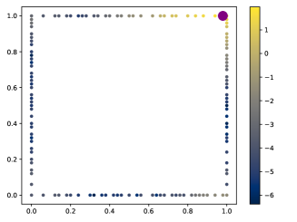
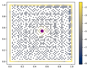
Figure 5: Demonstration of screening effects for the reduced kernel matrix. We choose the Matérn kernel with $\nu=5/2$; the lengthscale parameter is $0.3$. The data points are equidistributed in $[0,1]^{2}$ with grid size $h=0.02$. In the left figure, we show a boundary point, and all the points ordered before are marked with a color whose intensity scales with the entry value $|U_{ij}^{\star}|$. The right figure is obtained in the same manner but for an interior measurement.

From the left figure, we observe a desired screening effect for boundary Diracs measurements. However, in the right figure, we observe that the interior derivative-type measurements still exhibit a strong conditional correlation with boundary points. That means that the correlation with boundary points is not screened thoroughly. This also implies that the presence of the interior Diracs measurements is the key to the sparse Choleksy factors for the previous $K(\tilde{{\bm{\phi}}},\tilde{{\bm{\phi}}})^{-1}$.

The right of Figure 5 demonstrates a negative result: one cannot hope that the Cholesky factor of $\Theta^{-1}$ will be as sparse as before. However, algorithmically, we can still apply the sparse Cholesky factorization to the matrix. We present numerical experiments to test the accuracy of such factorization. In the right of Figure 4, we show the KL errors of the resulting factorization concerning the sparsity parameter $\rho$. Even though the screening effect is not perfect, as we discussed above, we still observe a consistent decay of the KL errors when $\rho$ increases.

In addition, although we cannot theoretically guarantee the factor is as accurate as before, we can use it as a preconditioner to solve linear systems involving $K({\bm{\phi}}^{k},{\bm{\phi}}^{k})$. In practice, we observe that this idea works very well, and nearly constant steps of preconditioned conjugate gradient (pCG) iterations can lead to an accurate solution to (20). As a demonstration, in Figure 6, we show the pCG iteration history when the preconditioning idea is employed. The stopping criterion for pCG is that the relative tolerance is smaller than $2^{-26}\approx 10^{-8}$, which is the default criterion in Julia. From the figures, we can see that pCG usually converges in 10-40 steps, and this fast convergence is insensitive to the numbers of points. When $\rho$ is large, the factor is more accurate, and the preconditioner is better, leading to smaller number of required pCG steps. Among all the cases, the number of pCG steps required to reach the stopping criterion is of the same magnitude, and is not large.

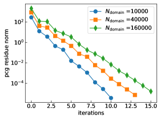
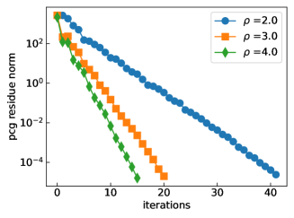
Figure 6: Demonstration of the convergence history of the pCG iteration. We choose the Matérn kernel with $\nu=5/2$; the lengthscale parameter is $0.3$. In the left figure, we choose the data points to be equidistributed in $[0,1]^{2}$ with different grid sizes; $\rho=4.0$. We show the equation residue norms of the iterates in each pCG iteration. In the right figure, we choose the data points to be equidistributed in $[0,1]^{2}$ with grid size $0.0025$ so that $N_{\rm domain}=160000$. We plot the pCG iteration history for $\rho=2.0,3.0,4.0$.

It is worth noting that since $K({\bm{\phi}}^{k},{\bm{\phi}}^{k})=DF(\mathbf{z}^{k})K({\bm{\phi}},{\bm{\phi}})(DF(\mathbf{z}^{k}))^{T}$ and we have a provably accurate sparse Cholesky factorization for $K({\bm{\phi}},{\bm{\phi}})^{-1}$, the matrix-vector multiplication for $K({\bm{\phi}}^{k},{\bm{\phi}}^{k})$ in each pCG iteration is efficient.

5.3 General case

The description in the last subsection applies directly to general nonlinear PDEs, which correspond to general ${\bm{\phi}}$ and $F$ in (7). We use the maximin ordering on the boundary, followed by the conditioned maximin ordering in the interior. We denote the ordering by $Q:I\to I$. The lengthscale is defined by

(21) $$l_{i}=\mathrm{dist}(\mathbf{x}_{Q(i)},\{\mathbf{x}_{Q(1)},...,\mathbf{x}_{Q(i-1)}\}\cup\mathsf{A})\,,$$

where for a boundary measurement, $\mathsf{A}=\emptyset$ and for an interior measurement $\mathsf{A}=\partial\Omega$. With the ordering and lengthscales, we create the sparse pattern through (11) (and aggregate it using the supernodes idea) and apply the KL minimization in Subsection 3.1 to obtain an approximate factor for $K({\bm{\phi}}^{k},{\bm{\phi}}^{k})^{-1}$. The general algorithmic procedure is outlined in Algorithm 2. We now denote the sparsity parameter for the reduced kernel matrix by $\rho_{\rm r}$.

Algorithm 2 Sparse Cholesky factorization for $K({\bm{\phi}}^{k},{\bm{\phi}}^{k})^{-1}$

Input: Measurements ${\bm{\phi}}^{k}$, kernel function $K$, sparsity parameter $\rho_{\rm r}$, supernodes parameter $\lambda$
Output: $U^{\rho_{\rm r}}_{\rm r},Q_{\rm perm}$

1:  Reordering and sparsity pattern: we first order the boundary measurements using the maximin ordering. Next, we order the interior measurements using the maximin ordering conditioned on $\partial\Omega$. This process yields a permutation matrix denoted by $Q_{\rm perm}$ such that $Q_{\rm perm}{\bm{\phi}}^{k}=\tilde{{\bm{\phi}}}^{k}$, and lengthscales $l$ for each measurement in $\tilde{{\bm{\phi}}}^{k}$. Under the ordering, we construct the aggregate sparsity pattern $S_{Q,l,\rho_{\rm r},\lambda}$ based on the chosen values of $\rho_{\rm r}$ and $\lambda$.

2:  KL minimization: solve (13) with $\Theta=K(\tilde{{\bm{\phi}}}^{k},\tilde{{\bm{\phi}}}^{k})$, by (14), to obtain $U^{\rho_{\rm r}}_{\rm r}$

3:  return  $U^{\rho_{\rm r}}_{\rm r},Q_{\rm perm}$

Now, putting all things together, we outline the general algorithmic procedure for solving the PDEs using the second-order Gauss-Newton method, in Algorithm 3.

Algorithm 3 Sparse Cholesky accelerated Gauss-Newton for solving (7)

Input: Measurements ${\bm{\phi}}$, data functional $F$, data vector $\mathbf{y}$, kernel function $K$, number of Gauss-Newton steps $t$, sparsity parameters $\rho,\rho_{\mathrm{r}}$, supernodes parameter $\lambda$
Output: Solution $\mathbf{z}^{t}$

1:  Factorize $K({\bm{\phi}},{\bm{\phi}})^{-1}\approx P_{\rm perm}^{T}U^{\rho}{U^{\rho}}^{T}P_{\rm perm}$ using Algorithm 1

2:  Set $k=0$, $\mathbf{z}^{k}=\textbf{0}$ or other user-specified initial guess

3:  while $k<t$ do

4:     Form the reduced measurements ${\bm{\phi}}^{k}=DF(\mathbf{z}^{k}){\bm{\phi}}$

5:     Factorize $K({\bm{\phi}}^{k},{\bm{\phi}}^{k})^{-1}$ to get $Q_{\rm perm}^{T}U_{\rm r}^{\rho_{\rm r}}{U_{\rm r}^{\rho_{\rm r}}}^{T}Q_{\rm perm}$ using Algorithm 2

6:     Use pCG to solve (20) with the preconditioner $Q_{\rm perm}^{T}U_{\rm r}^{\rho_{\rm r}}{U_{\rm r}^{\rho_{\rm r}}}^{T}Q_{\rm perm}$

7:     $\mathbf{z}^{k+1}=(P^{T}_{\rm perm}U^{\rho}{U^{\rho}}^{T}P_{\rm perm})\backslash((DF(\mathbf{z}^{k}))^{T}\gamma)$

8:     $k=k+1$

9:  end while

10:  return  $\mathbf{z}^{t}$

For the choice of parameters, we usually set $t$ to be between 2 to 10. Setting $\rho=O(\log(N/\epsilon))$ suffices to obtain an $\epsilon$-accurate approximation of $K({\bm{\phi}},{\bm{\phi}})^{-1}$. We do not have a theoretical guarantee for the factorization algorithm applied to the reduced kernel matrix $K({\bm{\phi}}^{k},{\bm{\phi}}^{k})^{-1}$. Still, our experience indicates that setting $\rho_{\rm r}=\rho$ or a constant such as $\rho_{\rm r}=3$ works well in practice. We note that a larger $\rho_{\rm r}$ increases the factorization time while decreasing the necessary pCG steps to solve the linear system, as demonstrated in the right of Figure 6. There is a trade-off here in general.

The overall complexity of Algorithm 3 for solving (18) is $O(N\log^{2}(N)\rho^{d}+N\rho^{2d}+Mt\rho_{\rm r}^{2d}+T_{\rm pCG})$ in time and $O(N\rho^{d}+M\rho_{\rm r}^{d})$ in space, where $O(N\log^{2}(N)\rho^{d})$ is the time for generating the ordering and sparsity pattern, $O(N\rho^{2d})$ is for the factorization, and $O(Mt\rho_{\rm r}^{2d})$ is for the factorizations in all the GN iterations, $T_{\rm pCG}$ is the time that the pCG iterations take.

Based on empirical observations, we have found that $T_{\rm pCG}$ scales nearly linearly with respect to $N\rho^{d}$. This is because a nearly constant number of pCG iterations are sufficient to obtain an accurate solution, and each pCG iteration takes at most $O(N\rho^{d})$ time, as explained in the matrix-vector multiplication mentioned at the end of Subsection 5.2. Additionally, it is worth noting that the time required for generating the ordering and sparsity pattern ($O(N\log^{2}(N)\rho^{d})$) is negligible in practice, compared to that for the KL minimization. Furthermore, the ordering and sparsity pattern can be pre-computed once and reused for multiple runs.

6 Numerical experiments

In this section, we use Algorithm 3 to solve nonlinear PDEs. The numerical experiments are conducted on the personal computer MacBook Pro 2.4 GHz Quad-Core Intel Core i5. In all the experiments, the physical data points are equidistributed on a grid; we specify its size in each example. We always set the sparsity parameter for the reduced kernel matrix $\rho_{\rm r}=\rho$, the sparsity parameter for the original matrix. We adopt the supernodes ideas in all the examples and set the parameter $\lambda=1.5$.

Our theory guarantees that once the Diracs measurements are ordered first by the maximin ordering, the derivative measurements can be ordered arbitrarily. In practice, for convenience, we order them from lower-order to high-order derivatives, and for the same type of derivatives, we order the corresponding measurements based on their locations, in the same maximin way as the Diracs measurements.

Our codes are in https://github.com/yifanc96/PDEs-GP-KoleskySolver.

6.1 Nonlinear elliptic PDEs

Our first example is the nonlinear elliptic equation

(22) $$\left\{\begin{aligned} -\Delta u+\tau(u)&=f\quad\text{in }\Omega\,,\\ u&=g\quad\text{on }\partial\Omega\,,\end{aligned}\right.$$

with $\tau(u)=u^{3}$. Here $\Omega=[0,1]^{2}$. We set

$$u(\mathbf{x})=\sum_{k=1}^{600}\frac{1}{k^{6}}\sin(k\pi x_{1})\sin(k\pi x_{2})$$

as the ground truth and use it to generate the boundary and right hand side data. We set the number of Gauss-Newton iterations to be 3. The initial guess for the iteration is a zero function. The lengthscale of the kernels is set to be $0.3$.

We first study the solution error and the CPU time regarding $\rho$. We choose the number of interior points to be $N_{\rm domain}=40000$; or equivalently, the grid size $h=0.005$. In the left side of Figure 7, we observe that a larger $\rho$ leads to a smaller $L^{2}$ error of the solution. For the Matérn kernel with $\nu=5/2,7/2$, we observe that such accuracy improvement saturates at $\rho=2$ or $4$, while when $\nu=7/2$. the accuracy keeps improving until $\rho=10$. This high accuracy for large $\nu$ is because the solution $u$ is fairly smooth. Using smoother kernels can lead to better approximation accuracy. On the other hand, smoother kernels usually need a larger $\rho$ to achieve the same level of approximation accuracy, as we have demonstrated in the left of Figure 3.

In the right side of Figure 7, we show the CPU time required to compute the solution for different kernels and $\rho$. A larger $\rho$ generally leads to a longer CPU time. But there are some exceptions: for the Matérn kernel with $\nu=5/2,7/2$, the CPU time for $\rho=3$ is longer than that for $\rho=2$. Again, the reason is that these smoother kernels often require a larger $\rho$ for accurate approximations. When $\rho$ is very small, although the sparse Cholesky factorization is very fast, the pCG iterations could take long since the preconditioner matrix does not approximate the matrix well.

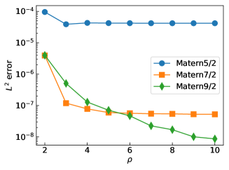
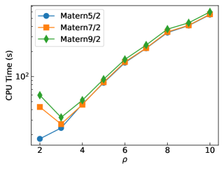
Figure 7: Nonlinear elliptic PDE example. The left figure concerns the $L^{2}$ errors of the solution, while the right figure concerns the CPU time. Both plots are with regard to $\rho$. We set $N_{\rm domain}=40000$.

We then study the $L^{2}$ errors and CPU time regarding the number of physical points. We fix $\rho=4.0$. In the left of Figure 8, we observe that the accuracy improves when $N_{\rm domain}$ increases. For the smoother Matérn kernels with $\nu=7/2,9/2$, they will hit an accuracy floor of $10^{-7}$. This is because we only have a finite number of Gauss-Newton steps and a finite $\rho$. In the right of Figure 8, a near-linear complexity in time regarding the number of points is demonstrated.

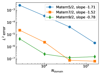
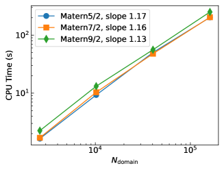
Figure 8: Nonlinear elliptic PDE example. The left figure concerns the $L^{2}$ errors of the solution, while the right figure concerns the CPU time. Both plots are with regard to the number of physical points in the domain. We set $\rho=4.0$.

6.2 Burgers’ equation

Our second example concerns the time-dependent Burgers equation:

(23) $$\partial_{t}u+u\partial_{x}u-0.001\partial_{x}^{2}u =0,\quad\forall(x,t)\in(-1,1)\times(0,1]\,,$$

$$u(x,0) =-\sin(\pi x)\,,$$

$$u(-1,t) =u(1,t)=0\,.$$

Rather than using a spatial-temporal GP as in [7], we first discretize the equation in time and then use a spatial GP to solve the resulting PDE in space. This reduces the dimensionality of the system and is more efficient. More precisely, we use the Crank–Nicolson scheme with time stepsize $\Delta t$ to obtain

(24) $$\frac{\hat{u}(x,t_{n+1})-\hat{u}(x,t_{n})}{\Delta t}+\frac{1}{2} \left(\hat{u}(x,t_{n+1})\partial_{x}\hat{u}(x,t_{n+1})+\hat{u}(x,t_{n})\partial_{x}\hat{u}(x,t_{n})\right)$$

$$=\frac{0.001}{2}\left(\partial_{x}^{2}\hat{u}(x,t_{n+1})+\partial_{x}^{2}\hat{u}(x,t_{n})\right)\,,$$

where $\hat{u}(t_{n},x)$ is an approximation of the true solution $u(t_{n},x)$ with $t_{n}=n\Delta t$. When $\hat{u}(\cdot,t_{n})$ is known, (24) is a spatial PDE for the function $\hat{u}(\cdot,t_{n+1})$. We can solve (24) iteratively starting from $n=0$. We use two steps of Gauss-Newton iterations with the initial guess as the solution at the last time step.

We set $\Delta t=0.02$ and compute the solution at $t=1$. The lengthscale of the kernels is chosen to be $0.02$. We set $\rho=4.0$ in the factorization algorithm. In the left of Figure 9, we show our numerical solution by using a grid of size $h=0.001$ and the true solution computed by using the Cole-Hopf transformation. We see that they match very well, and the shock is captured. This is possible because we use a grid of small size so that the shock is well resolved. With a very small grid size, we need to deal with many large-size dense kernel matrices, and we use the sparse Cholesky factorization algorithm to handle such a challenge.

In the right of Figure 9, we show the CPU time of our algorithm regarding different $N_{\rm domain}$. We clearly observe a near-linear complexity in time. The total CPU time is less than $10$ seconds to handle $50$ dense kernel matrices (since $1/\Delta t=50$) of size larger than $10^{4}$ (the dimension of $K({\bm{\phi}},{\bm{\phi}})$ is around $3\times N_{\rm domain}$ since we have three types of measurements) sequentially.

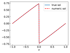
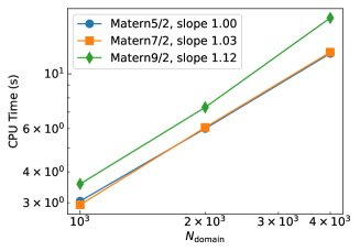
Figure 9: Burgers’ equation example. The left figure is a demonstration of the numerical solution and true solution at $t=1$. The right figure concerns the CPU time regarding the number of physical points. We set $\rho=4.0$.

We also show the accuracy of our solutions in the following Table 1.

$N_{\rm domain}$	$1000$	$2000$	$4000$
$L^{2}$ error	1.729e-4	6.111e-5	7.453e-5
$L^{\infty}$ error	1.075e-3	2.745e-4	1.075e-4

Table 1: Burgers’ equation example. The $L^{2}$ and $L^{\infty}$ errors of the computed solution at $t=1$. We use the Matérn kernel with $\nu=7/2$. The sparsity parameter $\rho=4.0$.

We observe high accuracy, $O(10^{-5})$ in the $L^{2}$ norm and $O(10^{-4})$ in the $L^{\infty}$ norm. The $L^{2}$ errors do not decrease when we increase the number of points from $2000$ to $4000$. It is because we use a fixed time stepsize $\Delta t=0.02$ and a fixed $\rho=4.0$.

6.3 Monge-Ampère equation

Our last example is the Monge-Ampère equation in two dimensional space.

(25) $$\operatorname{det}(D^{2}u)=f,\quad\mathbf{x}\in(0,1)^{2}\,.$$

Here, we choose $u(\mathbf{x})=\exp(0.5((x_{1}-0.5)^{2}+(x_{2}-0,5)^{2}))$ to generate the boundary and right hand side data. To ensure uniqueness of the solution, some convexity assumption is usually needed. Here, to test the wide applicability of our methodology, we directly implement Algorithm 3. We adopt $3$ steps of Gauss-Newton iterations with the initial guess $u(\mathbf{x})=\frac{1}{2}\|\mathbf{x}\|^{2}$. We choose the Matérn kernel with $\nu=5/2$. The lengthscale of the kernel is set to be $0.3$.

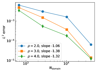
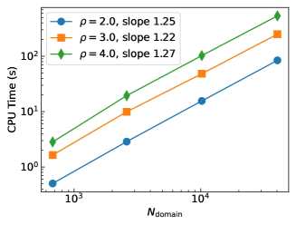
Figure 10: The Monge-Ampère equation example. The left figure concerns the $L^{2}$ errors, while the right figure concerns the CPU time. Both are with respect to the number of physical points in space, and in both figures, we consider $\rho=2.0,3.0,4.0$. We choose the Matérn kernel with $\nu=5/2$ in this example.

In Figure 10, we present the $L^{2}$ errors of the solution and the CPU time with respect to $N_{\rm domain}$. Once again, we observe a nearly linear complexity in time. However, since $\det(D^{2}u)$ involves several partial derivatives of the function, we need to differentiate our kernels accordingly; we use auto-differentiation in Julia for convenience, which is slightly slower than the hand-coded derivatives used in our previous numerical examples. Consequently, the total CPU time is longer compared to the earlier examples, although the scaling regarding $N_{\rm domain}$ remains similar.

As $N_{\rm domain}$ increases, the $L^{2}$ solution errors decrease for $\rho=2.0,3.0,4.0$. This indicates that our kernel method is convergent for such a fully nonlinear PDE. However, since we do not incorporate singularity into the solution, this example may not correspond to the most challenging setting. Nonetheless, the success of this simple methodology combined with systematic fast solvers demonstrates its potential for promising automation and broader applications in solving nonlinear PDEs.

7 Conclusions

In this paper, we have investigated a sparse Cholesky factorization algorithm that enables scaling up the GP method for solving nonlinear PDEs. Our algorithm relies on a novel ordering of the Diracs and derivative-type measurements that arise in the GP-PDE methodology. With this ordering, the Cholesky factor of the inverse kernel matrix becomes approximately sparse, and we can use efficient KL minimization, equivalent to Vecchia approximation, to compute the sparse factors. We have provided rigorous analysis of the approximation accuracy by showing the exponential decay of the conditional covariance of GPs and the Cholesky factors of the inverse kernel matrix, for a wide class of kernel functions and derivative measurements.

When using second-order Gauss-Newton methods to solve the nonlinear PDEs, a reduced kernel matrix arises, in which many interior Dirac measurements are absent. In such cases, the decay is weakened, and the accuracy of the factorization deteriorates. To compensate for this loss of accuracy, we use pCG iterations with this approximate factor as a preconditioner. In our numerical experiments, our algorithm achieves high accuracy, and the computation time scales near-linearly with the number of points. This justifies the potential of GPs for solving general PDEs with automation, efficiency, and accuracy. We anticipate extending our algorithms to solving inverse problems and our theories to more kernel functions and measurement functionals in the future.

Appendix A Supernodes and aggregate sparsity pattern

The supernode idea is adopted from [61], which allows to re-use the Cholesky factors in the computation of (14) to update multiple columns at once.

We group the measurements into supernodes consisting of measurements whose points are close in location and have similar lengthscale parameters $l_{i}$. To do this, we select the last index $j\in I$ of the measurements in the ordering that has not been aggregated into a supernode yet and aggregate the indices in $\{i:(i,j)\in S_{P,l,\rho},l_{i}\leq\lambda l_{j}\}$ that have not been aggregated yet into a common supernode, for some $\lambda>1$. We repeat this procedure until every measurement has been aggregated into a supernode. We denote the set of all supernodes as $\tilde{I}$ and write $i\leadsto\tilde{i}$ for $i\in I$ and $\tilde{i}\in\tilde{I}$ if $\tilde{i}$ is the supernode to which $i$ has been aggregated.

The idea is to assign the same sparsity pattern to all the measurements of the same supernode. To achieve so, we define the sparsity set for a supernode as the union of the sparsity sets of all the nodes it contains, namely $s_{\tilde{i}}:=\{j:\exists i\leadsto\tilde{i},j\in s_{i}\}$. Then, we introduce the aggregated sparsity pattern

$$S_{P,l,\rho,\lambda}:=\bigcup_{\tilde{j}}\bigcup_{j\leadsto\tilde{j}}\{(i,j)\subset I\times I:i\leq j,i\in s_{\tilde{j}}\}\,.$$

Under mild assumptions (Theorem B.5 in [61]), one can show that there are $O(N/\rho^{d})$ number of supernodes and each supernode contains $O(\rho^{d})$ measurements. The size of the sparsity set for a supernode $\#s_{\tilde{j}}=O(\rho^{d})$. For a visual demonstration of the grouping and aggregate sparsity pattern, see Figure 11, which is taken from Figure 3 in [61].

Figure 11: The figure on the left illustrates the original pattern $S_{P,\ell,\rho}$. For each orange point $j$, its sparsity pattern $s_{j}$ includes all points within a circle with a radius of $\rho$. On the right, all points $j$ that are located close to each other and have similar lengthscales are grouped into a supernode $\tilde{j}$. The supernode can be represented by a list of parents (the orange points within an inner sphere of radius $\approx\rho$, or all $j\leadsto\tilde{j}$) and children (all points within a radius $\leq 2\rho$, which correspond to the sparsity set $s_{\tilde{j}}$). Figure reproduced from [61] with author permission.

Now, we can compute (14) with the aggregated sparsity pattern more efficiently. Let $s_{j}^{*}=\{i:(i,j)\in S_{P,l,\rho,\lambda}\}$ be the individual sparsity pattern for $j$ in the aggregated pattern $S_{P,l,\rho,\lambda}$. In (14), we need to compute matrix-vector products for $\Theta_{s_{j}^{*},s_{j}^{*}}^{-1}$. For that purpose, one can apply the Cholesky factorization to $\Theta_{s_{j}^{*},s_{j}^{*}}$. Naïvely computing Cholesky factorizations of every $\Theta_{s_{j}^{*},s_{j}^{*}}$ will result in $O(N\rho^{3d})$ arithmetic complexity. However, due to the supernode construction, we can factorize $\Theta_{s_{\tilde{j}},s_{\tilde{j}}}$ once and then use the resulting factor to obtain the Cholesky factors of $\Theta_{s_{j}^{*},s_{j}^{*}}$ directly for all $j\leadsto\tilde{j}$. This is because our construction guarantees that

$$\Theta_{s_{j}^{*},s_{j}^{*}}=\Theta_{s_{\tilde{j}},s_{\tilde{j}}}[1:\#s_{j}^{*},1:\#s_{j}^{*}]\,,$$

where we used the MATLAB notation. The above relation shows that sub-Cholesky factors of $\Theta_{s_{\tilde{j}},s_{\tilde{j}}}$ become the Cholesky factors of $\Theta_{s_{j}^{*},s_{j}^{*}}$ for $j\leadsto\tilde{j}$.

Therefore, one step of Cholesky factorization works for all $O(\rho^{d})$ measurements in the supernode. In total, the arithmetic complexity is upper bounded by $O(\rho^{3d}\times N/\rho^{d})=O(N\rho^{2d})$. For more details of the algorithm, we refer to section 3.2, in particular Algorithm 3.2, in [61].

It was shown that the aggregate sparsity pattern could be constructed with time complexity $O(N\log(N)+N\rho^{d})$ and space complexity $O(N)$; see Theorem C.3 in [61]. They are of a lower order compared to the time complexity $O(N\log^{2}(N)\rho^{d})$ and space complexity $O(N\rho^{d})$ for generating the maximin ordering and the original sparsity pattern $S_{P,l,\rho}$ (see Remark LABEL:rmk:_complexity_maximin_ordering_sparsity_patterns).

Appendix B Ball-packing arguments

The ball-packing argument is useful to bound the cardinality of the sparsity pattern.

Proposition B.1.

Consider the maximin ordering (Definition 3.2) and the sparsity pattern defined in (11). For each column $j$, denote $s_{j}=\{i:(i,j)\in S_{P,l,\rho}\}$. The cardinality of the set $s_{j}$ is denoted by $\#s_{j}$. Then, it holds that $\#s_{j}=O(\rho^{d})$.

Proof B.2.

Fix a $j$. For any $i\in s_{j}$, we have $\operatorname{dist}(\mathbf{x}_{P(i)},\mathbf{x}_{P(j)})\leq\rho l_{j}$. Moreover, by the definition of the maximin ordering, we know that for $i,i^{\prime}\in s_{j}$ and $i\neq i^{\prime}$, it holds that $\operatorname{dist}(\mathbf{x}_{P(i)},\mathbf{x}_{P(i^{\prime})})\geq l_{j}$. Thus, the cardinality of $s_{i}$ is bounded by the number of disjoint balls of radius $l_{j}$ that the ball $B(\mathbf{x}_{P(i)},2\rho l_{j})$ can contain. Clearly, $\#s_{i}=O(\rho^{d})$. The proof is complete.

Appendix C Explicit formula for the KL minimization

By direct calculation, one can show the KL minimization attains an explicit formula. The proof of this explicit formula follows a similar approach to that of Theorem 2.1 in [61], with the only difference being the use of upper Cholesky factors.

Proposition C.1.

The solution to (13) is given by (14).

Proof C.2.

We use the explicit formula for the KL divergence between two multivariate Gaussians:

(26) $$\operatorname{KL}\left(\mathcal{N}(0,\Theta)\parallel\mathcal{N}(0,(UU^{T})^{-1})\right)$$

$$= \frac{1}{2}[-\log\det(U^{T}\Theta U)+\operatorname{tr}(U^{T}\Theta U)-N]\,.$$

To identify the minimizer, the constant and scaling do not matter, so we focus on the $-\log\det(U^{T}\Theta U)$ and $\operatorname{tr}(U^{T}\Theta U)$ parts. By writing $U=[U_{:,1},...,U_{:,M}]$, we get

(27) $$-\log\det(U^{T}\Theta U)+\operatorname{tr}(U^{T}\Theta U)=\sum_{j=1}^{M}[-2\log U_{jj}+\operatorname{tr}(U_{:,j}^{T}\Theta U_{:,j})]-\log\det\Theta\,.$$

Thus the minimization is decoupled to each column of $U$. Due to the choice of the sparse pattern, we have $U_{:,j}^{T}\Theta U_{:,j}=U_{s_{j},j}^{T}\Theta_{s_{j},s_{j}}U_{s_{j},j}$. We can further simplify the formula

(28) $$\operatorname{tr}(U_{:,j}^{T}\Theta U_{:,j})=\operatorname{tr}(U_{s_{j},j}^{T}\Theta_{s_{j},s_{j}}U_{s_{j},j})\,.$$

It suffices to identify the minimizer of $-2\log U_{jj}+\operatorname{tr}(U_{s_{j},j}^{T}\Theta_{s_{j},s_{j}}U_{s_{j},j})$. Taking the derivatives, we get the optimality condition:

(29) $$-\frac{2}{U_{jj}}\textbf{e}_{\#s_{j}}+2\Theta_{s_{j},s_{j}}U_{s_{j},j}=0\,,$$

where $\textbf{e}_{\#s_{j}}$ is a standard basis vector in $\mathbb{R}^{\#s_{j}}$ with the last entry being $1$ and other entries equal $0$.

Solving this equation leads to the solution

(30) $$U_{s_{j},j}=\frac{\Theta_{s_{j},s_{j}}^{-1}\textbf{e}_{\#s_{j}}}{\sqrt{\textbf{e}_{\#s_{j}}^{T}\Theta_{s_{j},s_{j}}^{-1}\textbf{e}_{\#s_{j}}}}\,.$$

The proof is complete.

Appendix D Proofs of the main theoretical results

D.1 Proof of Theorem 4.1

Proof D.1 (Proof of Theorem 4.1).

We rely on the interplay between GP regression, linear algebra, and numerical homogenization to prove this theorem. Consider the GP $\xi\sim\mathcal{N}(0,\mathcal{L}^{-1})$. For each measurement functional, we define the Gaussian random variables $Y_{i}=[\xi,\tilde{\phi}_{i}]\sim\mathcal{N}(0,[\tilde{\phi}_{i},\mathcal{L}^{-1}\tilde{\phi}_{i}])=\mathcal{N}(0,\Theta_{ii})$. As mentioned in Remark LABEL:remark:_why_coarse-to-fine_ordering and proved in Proposition D.7, we have a relation between the Cholesky factor and the GP conditioning, as

$$\frac{U^{\star}_{ij}}{U^{\star}_{jj}}=(-1)^{i\neq j}\frac{\mathrm{Cov}[Y_{i},Y_{j}|Y_{1:j-1\backslash\{i\}}]}{\mathrm{Var}[Y_{i}|Y_{1:j-1\backslash\{i\}}]},i\leq j\,.$$

Moreover, by Proposition D.9, one can connect the conditional covariance of GPs with conditional expectation, such that

(31) $$\frac{\mathrm{Cov}[Y_{i},Y_{j}|Y_{1:j-1\backslash\{i\}}]}{\mathrm{Var}[Y_{i}|Y_{1:j-1\backslash\{i\}}]}=\mathbb{E}[Y_{j}|Y_{i}=1,Y_{1:j-1\backslash\{i\}}=0]\,.$$

The above conditional expectation is related to the Gamblets introduced in the numerical homogenization literature. Indeed, using the relation $Y_{i}=[\xi,\tilde{\phi}_{i}]$, we have

(32) $$\mathbb{E}[Y_{j}|Y_{i}=1,Y_{1:j-1\backslash\{i\}}=0]=[\mathbb{E}[\xi|Y_{i}=1,Y_{1:j-1\backslash\{i\}}=0],\tilde{\phi}_{j}]=[\psi_{j}^{i},\tilde{\phi}_{j}]\,,$$

where $\psi_{j}^{i}(\mathbf{x}):=\mathbb{E}[\xi(\mathbf{x})|Y_{i}=1,Y_{1:j-1\backslash\{i\}}=0]$; it is named Gamblets in [48, 49].

Importantly, for the conditional expectation, by Proposition D.11, we have the following variational characterization [48, 49]:

(33) $$\psi_{j}^{i}=\text{argmin}_{\psi\in H_{0}^{s}(\Omega)} [\psi,\mathcal{L}\psi]$$

subject to $$[\psi,\tilde{\phi}_{k}]=\delta_{i,k}\ \ \text{for}\ \ 1\leq k\leq j-1\,.$$

A main property of the Gamblets is that they can exhibit an exponential decay property under suitable assumptions, which can be used to prove our theorem. We collect the related theoretical results in Appendix D.4; we will use them in our proof.

Our proof for the theorem consists of two steps. The first step is to bound $|{U^{\star}_{ij}}/{U^{\star}_{jj}}|$, and the second step is to bound $|U_{jj}^{*}|$.

For the first step, we separate the cases $j\leq M$ and $j>M$. Indeed, the case $j\leq M$ has been covered in [62, 61]. Here, our proof is simplified.

For $1\leq i\leq j\leq M$, by the discussions above, we have the relation:

(34) $$\left|\frac{U^{\star}_{ij}}{U^{\star}_{jj}}\right|=\left|[\psi_{j}^{i},\tilde{\phi}_{j}]\right|=|\psi_{j}^{i}(\mathbf{x}_{P(j)})|\,,$$

where we used the fact that $\tilde{\phi}_{j}=\updelta_{\mathbf{x}_{P(j)}}$ because all the Diracs measurements are ordered first. To bound $|\psi_{j}^{i}(\mathbf{x}_{P(j)})|$, we will use the exponential decay results for Gamblets that we prove in Proposition D.17. More precisely, to apply Proposition D.17 to this context, we need to verify its assumptions, especially Assumption 2.

In our setting, we can construct a partition of the domain $\Omega$ by using the Voronoi diagram. Denote $X_{j-1}=\{\mathbf{x}_{P(1)},...,\mathbf{x}_{P(j-1)}\}$. We note that $X_{M}$ will consist of all the physical points. We define $\tau_{k}$, for $1\leq k\leq j-1$, to be the Voronoi cell, which contains all points in $\Omega$ that is closer to $\mathbf{x}_{P(k)}$ than to any other in $X_{j-1}$. Since we assume $\Omega$ is convex, $\tau_{k}$ is also convex. And bounded convex domains are uniform Lipschitz.

Furthermore, to verify the other parts in Assumption 2, we analyze the homogeneity parameter of $X_{j-1}$. By definition,

(35) $$\delta(X_{j-1};\partial\Omega)=\frac{\min_{\mathbf{x},\mathbf{y}\in X_{j-1}}\mathrm{dist}(\mathbf{x},\{\mathbf{y}\}\cup\partial\Omega)}{\max_{\mathbf{x}\in\Omega}\mathrm{dist}(\mathbf{x},X_{j-1}\cup\partial\Omega)}\,.$$

By definition of the maximin ordering, we have

(36) $$\min_{\mathbf{x},\mathbf{y}\in X_{j-1}}\mathrm{dist}(\mathbf{x},\{\mathbf{y}\}\cup\partial\Omega)=l_{j-1}\,.$$

Then, by the triangle inequality, it holds that

(37) $$\max_{\mathbf{x}\in\Omega}\mathrm{dist}(\mathbf{x},X_{j-1}\cup\partial\Omega) \leq\max_{\mathbf{x}\in X_{M}}\mathrm{dist}(\mathbf{x},X_{j-1}\cup\partial\Omega)+\max_{\mathbf{x}\in\Omega}\mathrm{dist}(\mathbf{x},X_{M})$$

$$\leq l_{j}+l_{M}/\delta(X_{M};\partial\Omega)\leq(1+1/\delta(X_{M};\partial\Omega))l_{j}\,,$$

where in the second inequality, we used the definition of the lengthscales $l_{j}$ and the homogeneity assumption of $X_{M}$ (i.e., $\delta(X_{M};\partial\Omega)>0$). Combining the above two estimates, we get $\delta(X_{j-1};\partial\Omega)\geq 1/(1+1/\delta(X_{M};\partial\Omega))>0$ where we used the fact that $l_{j}\leq l_{j-1}$. So $X_{j-1}$ is also homogeneously distributed with $\delta(X_{j-1};\partial\Omega)>0$.

We are ready to verify Assumption 2. Firstly, the balls $B(\mathbf{x},l_{j}/2),\mathbf{x}\in X_{j-1}$ do not intersect, and thus inside each $\tau_{k}$, there is a ball of center $\mathbf{x}_{P(k)}$ and radius $l_{j}/2$. Secondly, since $\max_{\mathbf{x}\in\Omega}\mathrm{dist}(\mathbf{x},X_{j-1}\cup\partial\Omega)\leq(1+1/\delta(X_{M};\partial\Omega))l_{j}$, we know that $\tau_{i}$ is contained in a ball of center $\mathbf{x}_{P(k)}$ and radius $(1+1/\delta(X_{M};\partial\Omega))l_{j}$. Therefore, Assumption 2 holds with $h=l_{j}/2$, $\delta=\min(1/(2+2/\delta(X_{M};\partial\Omega)),1)$ and $Q=j-1$. Assumption 3 readily holds by our choice of measurements.

Thus, applying Proposition D.17, we then get

(38) $$\left|\frac{U^{\star}_{ij}}{U^{\star}_{jj}}\right|=|\psi_{j}^{i}(\mathbf{x}_{P(j)})|\leq Cl_{j}^{-2s}\exp\left(-\frac{\mathrm{dist}(\mathbf{x}_{P(i)},\mathbf{x}_{P(j)})}{Cl_{j}}\right)\,,$$

where $C$ is a constant depending on $\Omega,\delta,d,s,\|\mathcal{L}\|,\|\mathcal{L}^{-1}\|$. We obtain the exponential decay of $|{U^{\star}_{ij}}/{U^{\star}_{jj}}|$ for $j\leq M$.

For $j>M$ and $i\leq j$, we have

(39) $$\left|\frac{U^{\star}_{ij}}{U^{\star}_{jj}}\right|=\left|[\psi_{j}^{i},\tilde{\phi}_{j}]\right|\leq\max_{0\leq|\gamma|\leq J}\left|D^{J}\psi_{j}^{i}(\mathbf{x}_{P(j)})\right|\,,$$

where we used the fact that $\tilde{\phi}_{j}$ is of the form $\updelta_{\mathbf{x}_{P(j)}}\circ D^{\gamma}$. Now, for $\psi_{j}^{i}$, the set of points we need to deal with is $X_{M}$. Similar to the case $j\leq M$, we define $\tau_{k}$, for $1\leq k\leq M$, to be the Voronoi cell of these points in $\Omega$. Then, using the same arguments in the previous case, we know that Assumption 2 holds with $h=l_{M}/2$, $\delta=\min(\delta(X_{M};\partial\Omega)/2,1)$ and $Q=M$. Assumption 3 readily holds by our choice of measurements. Therefore Proposition D.17 implies that

(40) $$\max_{0\leq|\gamma|\leq J}\left|D^{J}\psi_{j}^{i}(\mathbf{x}_{P(j)})\right|\leq Cl_{M}^{-2s}\exp\left(-\frac{\mathrm{dist}(\mathbf{x}_{P(i)},\mathbf{x}_{P(j)})}{Cl_{M}}\right)\,,$$

where $C$ is a constant depending on $\Omega,\delta,d,s,\|\mathcal{L}\|,\|\mathcal{L}^{-1}\|,J$.

Summarizing the above arguments, we have obtained that

(41) $$\left|\frac{U^{\star}_{ij}}{U^{\star}_{jj}}\right|\leq Cl_{j}^{-2s}\exp\left(-\frac{\mathrm{dist}(\mathbf{x}_{P(i)},\mathbf{x}_{P(j)})}{Cl_{j}}\right)\,,$$

for any $1\leq i\leq j\leq N$, noting that by our definition $l_{j}=l_{M}$ for $j>M$.

Now, we analyze $|U_{jj}^{*}|$. Note that $\Theta=K(\tilde{{\bm{\phi}}},\tilde{{\bm{\phi}}})\in\mathbb{R}^{N\times N}$ and $\Theta^{-1}=U^{\star}{U^{\star}}^{T}$. By the arguments above, we know that the assumptions in Proposition E.1 are satisfied with $h=l_{M}/2$, $\delta=\min(\delta(X_{M};\partial\Omega)/2,1)$ and $Q=M$. Thus, for any vector $w\in\mathbb{R}^{N}$, by Proposition E.1, we have

$$w^{T}\Theta^{-1}w\leq Cl_{M}^{-2s+d}|w|^{2}\,,$$

for some constant $C$ depending on $\delta(X_{M}),d,s,\|\mathcal{L}\|,J$. This implies that

$$|{U^{\star}}^{T}w|^{2}\leq Cl_{M}^{-2s+d}|w|^{2}\,.$$

Taking $w$ to be the standard basis vector $\textbf{e}_{j}$, we get

$$\sum_{k=j}^{N}|{U^{\star}_{jk}}|^{2}\leq Cl_{M}^{-2s+d}\,,$$

which leads to $|U_{ij}^{\star}|\leq Cl_{M}^{-s+d/2}$ for some $C$ depending on $\delta(X_{M};\partial\Omega),d,s,\|\mathcal{L}\|,J$.

D.2 Proof of Theorem 4.2

We need the following lemma, which is taken from Lemma B.8 in [61].

Lemma D.2.

Let $\lambda_{\min},\lambda_{\max}$ be the minimal and maximal eigenvalues of $\Theta\in\mathbb{R}^{N\times N}$, respectively. Then there exists a universal constant $\eta>0$ such that for any matrix $M\in\mathbb{R}^{N\times N}$, we have

• If $\lambda_{\max}\|\Theta^{-1}-MM^{T}\|_{\mathrm{Fro}}\leq\eta$, then

  $$\operatorname{KL}\left(\mathcal{N}(0,\Theta)\parallel\mathcal{N}(0,(MM^{T})^{-1})\right)\leq\lambda_{\max}\|\Theta^{-1}-MM^{T}\|_{\mathrm{Fro}}\,;$$

• If $\operatorname{KL}\left(\mathcal{N}(0,\Theta)\parallel\mathcal{N}(0,(MM^{T})^{-1})\right)\leq\eta$, then

  $$\|\Theta^{-1}-MM^{T}\|_{\mathrm{Fro}}\leq\lambda_{\min}^{-1}\operatorname{KL}\left(\mathcal{N}(0,\Theta)\parallel\mathcal{N}(0,(MM^{T})^{-1})\right)\,.$$

With this lemma, we can prove Theorem 4.2. The proof is similar to that of Theorem B.6 in [61].

Proof D.3 (Proof of Theorem 4.2).

First, by a covering argument, we know $l_{M}=O(M^{-1/d})=O(N^{-1/d})$. By Proposition E.1 with $h=l_{M}/2$, we know that

(42) $$\lambda_{\max}(\Theta)\leq C_{1}N\quad\mathrm{and}\quad\lambda_{\min}(\Theta)\geq C_{1}N^{-2s/d+1}$$

for some constant $C_{1}$ depending on $\delta(\{\mathbf{x}_{i}\}_{i\in I};\partial\Omega),d,s,\|\mathcal{L}\|,\|\mathcal{L}^{-1}\|,J$.

Theorem 4.1 implies that for $(i,j)\notin S_{P,l,\rho}$, it holds that

$$|U_{ij}^{\star}|\leq Cl_{M}^{-s+d/2}l_{j}^{-2s}\exp\left(-\frac{\mathrm{dist}(\mathbf{x}_{P(i)},\mathbf{x}_{P(j)})}{Cl_{j}}\right)\leq CN^{\alpha}\exp\left(-\frac{\rho}{C}\right)\,,$$

for some $\alpha$ depending on $s,d$, where $C$ is a generic constant that depends on $\Omega$, $\delta(\{\mathbf{x}_{i}\}_{i\in I};\partial\Omega),d,s,J,\|\mathcal{L}\|,\|\mathcal{L}^{-1}\|$. Moreover, from the proof in the last subsection, we know that $|U_{ij}^{*}|\leq CN^{s/d-1/2}$ for all $1\leq i\leq j\leq N$.

Now, consider the upper triangular Cholesky factorization $\Theta^{-1}=U^{\star}{U^{\star}}^{T}$. Define $M^{\rho}\in\mathbb{R}^{N\times N}$ such that

(43) $$M^{\rho}_{ij}=\begin{cases}U^{\star}_{ij},&\text{if }(i,j)\in S_{P,l,\rho}\\ 0,&\text{otherwise}\,.\end{cases}$$

Then, by using the above bounds on $U_{ij}^{\star}$, we know that there exists a constant $\beta$ depending on $s,d$, such that

(44) $$\|\Theta^{-1}-M^{\rho}{M^{\rho}}^{T}\|_{\mathrm{Fro}}\leq CN^{\beta}\exp\left(-\frac{\rho}{C}\right)\,.$$

Since $\lambda_{\max}(\Theta)\leq C_{1}N$, we know that there exists a constant $C^{\prime}$, such that when $\rho\geq C^{\prime}\log(N)$,

$$\lambda_{\max}(\Theta)\|\Theta^{-1}-M^{\rho}{M^{\rho}}^{T}\|_{\mathrm{Fro}}\leq\eta\,,$$

for the $\eta$ defined in Lemma D.2. Using Lemma D.2, we get

$$\operatorname{KL}\left(\mathcal{N}(0,\Theta)\parallel\mathcal{N}(0,(M^{\rho}{M^{\rho}}^{T})^{-1})\right)\leq\lambda_{\max}(\Theta)\|\Theta^{-1}-M^{\rho}{M^{\rho}}^{T}\|_{\mathrm{Fro}}\,.$$

By the KL optimality, the optimal solution $U^{\rho}$ will satisfy

(45) $$\operatorname{KL}\left(\mathcal{N}(0,\Theta)\parallel\mathcal{N}(0,(U^{\rho}{U^{\rho}}^{T})^{-1})\right)\leq\lambda_{\max}(\Theta)\|\Theta^{-1}-M^{\rho}{M^{\rho}}^{T}\|_{\mathrm{Fro}}\,.$$

Again by Lemma D.2, we get

(46) $$\|\Theta^{-1}-U^{\rho}{U^{\rho}}^{T}\|_{\mathrm{Fro}}\leq\frac{\lambda_{\max}(\Theta)}{\lambda_{\min}(\Theta)}\|\Theta^{-1}-M^{\rho}{M^{\rho}}^{T}\|_{\mathrm{Fro}}\,.$$

Moreover,

(47) $$\|\Theta-(U^{\rho}{U^{\rho}}^{T})^{-1}\|_{\mathrm{Fro}}\leq\|\Theta^{-1}\|_{\mathrm{Fro}}\|\Theta^{-1}-U^{\rho}{U^{\rho}}^{T}\|_{\mathrm{Fro}}\|U^{\rho}{U^{\rho}}^{T}\|_{\mathrm{Fro}}\,.$$

Using (44), (45), (46), and (47), and the fact that $\lambda_{\max}(\Theta),\lambda_{\min}(\Theta)$ are of polynomial growth in $N$ according to (42), we know that there exists a constant $C$ depending on $\Omega,\delta(\{\mathbf{x}_{i}\}_{i\in I};\partial\Omega),d,s,J,\|\mathcal{L}\|,$ $\|\mathcal{L}^{-1}\|$, such that when $\rho\geq C\log(N/\epsilon)$, it holds that

$$\operatorname{KL}\left(\mathcal{N}(0,\Theta)\parallel\mathcal{N}(0,(U^{\rho}{U^{\rho}}^{T})^{-1})\right)+\|\Theta^{-1}-U^{\rho}{U^{\rho}}^{T}\|_{\mathrm{Fro}}+\|\Theta-(U^{\rho}{U^{\rho}}^{T})^{-1}\|_{\mathrm{Fro}}\leq\epsilon\,.$$

The proof is complete.

D.3 Connections between Cholesky factors, conditional covariance, conditional expectation, and Gamblets

We first present two lemmas.

The first lemma is about the inverse of a block matrix [39].

Lemma D.4.

For a positive definite matrix $\Theta\in\mathbb{R}^{N\times N}$, if we write it in the block form

(48) $$\Theta=\begin{pmatrix}\Theta_{YY}&\Theta_{YZ}\\ \Theta_{ZY}&\Theta_{ZZ}\end{pmatrix}\,,$$

then, $\Theta^{-1}$ equals

(49) $$\begin{pmatrix}(\Theta_{YY}-\Theta_{YZ}\Theta_{ZZ}^{-1}\Theta_{ZY})^{-1}&-\Theta_{YY}^{-1}\Theta_{YZ}(\Theta_{ZZ}-\Theta_{ZY}\Theta_{YY}^{-1}\Theta_{YZ})^{-1}\\ -\Theta_{ZZ}^{-1}\Theta_{ZY}(\Theta_{YY}-\Theta_{YZ}\Theta_{ZZ}^{-1}\Theta_{ZY})^{-1}&(\Theta_{ZZ}-\Theta_{ZY}\Theta_{YY}^{-1}\Theta_{YZ})^{-1}\end{pmatrix}\,.$$

The second lemma is about the relation between the conditional covariance of a Gaussian random vector and the precision matrix.

Lemma D.5.

Let $N\geq 3$ and $X=(X_{1},...,X_{N})$ be a $\mathcal{N}(0,\Theta)$ Gaussian vector in $\mathbb{R}^{N}$. Let $Y=(X_{1},X_{2})$ and $Z=(X_{3},...,X_{N})$. Then,

(50) $$\mathrm{Cov}(Y_{1},Y_{2}|Z)=\frac{-A_{12}}{A_{11}A_{22}-A_{12}^{2}}\,,$$

and

(51) $$\mathrm{Var}(Y_{1}|Z)=\frac{A_{22}}{A_{11}A_{22}-A_{12}^{2}}\,,$$

where $A=\Theta^{-1}$. Therefore

(52) $$\frac{\mathrm{Cov}(Y_{1},Y_{2}|Z)}{\mathrm{Var}(Y_{1}|Z)}=\frac{-A_{12}}{A_{22}}\,.$$

Proof D.6.

First, we know that $\mathrm{Cov}(Y|Z)=\Theta_{YY}-\Theta_{YZ}\Theta_{ZZ}^{-1}\Theta_{ZY}$. By Lemma D.4, we have

(53) $$\Theta_{YY}-\Theta_{YZ}\Theta_{ZZ}^{-1}\Theta_{ZY}=\begin{pmatrix}A_{11}&A_{12}\\ A_{21}&A_{22}\end{pmatrix}^{-1}\,.$$

Inverting this matrix leads to the desired result.

With these lemmas, we can show the connection between the Cholesky factors and the conditional covariance as follows.

Proposition D.7.

Consider the positive definite matrix $\Theta\in\mathbb{R}^{N\times N}$. Suppose the upper triangular Cholesky factorization of its inverse is $U$, such that $\Theta^{-1}=UU^{T}$. Let $Y$ be a Gaussian vector with law $\mathcal{N}(0,\Theta)$. Then, we have

(54) $$\frac{U_{ij}}{U_{jj}}=(-1)^{i\neq j}\frac{\mathrm{Cov}[Y_{i},Y_{j}|Y_{1:j-1\backslash\{i\}}]}{\mathrm{Var}[Y_{i}|Y_{1:j-1\backslash\{i\}}]},\quad i\leq j\,.$$

Proof D.8.

We only need to consider the case $i\neq j$. We consider $j=N$ first. Denote $A=\Theta^{-1}$. By the definition of the Cholesky factorization $A=UU^{T}$, we know that $U_{:,N}=A_{:,N}/\sqrt{A_{NN}}$. Thus,

$$\frac{U_{iN}}{U_{NN}}=\frac{A_{iN}}{A_{NN}}\,.$$

For $i\neq N$, by Lemma D.5, we have

(55) $$\frac{\mathrm{Cov}[Y_{i},Y_{N}|Y_{1:N-1\backslash\{i\}}]}{\mathrm{Var}[Y_{i}|Y_{1:N-1\backslash\{i\}}]}=\frac{-A_{iN}}{A_{NN}}\,.$$

By comparing the above two identities, we obtain the result holds for $j=N$.

For $j<N$, we can use mathematical induction. Note that $U_{1:N-1,1:N-1}$ is also the upper triangular Cholesky factor of $(\Theta_{1:N-1,1:N-1})^{-1}$, noting the fact (by applying Lemma D.4 to the matrix $A$) that

$$(\Theta_{1:N-1,1:N-1})^{-1}=A_{1:N-1,1:N-1}-A_{1:N-1,N}A_{NN}^{-1}A_{N,1:N-1}$$

is the Schur complement, which is exactly the residue block in the Cholesky factorization. Therefore, applying the result for $j=N$ to the matrix $\Theta_{1:N-1,1:N-1}$, we prove (54) holds for $j=N-1$ as well. Iterating this process to $j=1$ finishes the proof.

Furthermore, the conditional covariance is related to the conditional expectation, as follows.

Proposition D.9.

For a Gaussian vector $Y\sim\mathcal{N}(0,\Theta)$, we have

(56) $$\frac{\mathrm{Cov}[Y_{i},Y_{j}|Y_{1:j-1\backslash\{i\}}]}{\mathrm{Var}[Y_{i}|Y_{1:j-1\backslash\{i\}}]}=\mathbb{E}[Y_{j}|Y_{i}=1,Y_{1:j-1\backslash\{i\}}=0]\,.$$

Proof D.10.

We show that for any zero-mean Gaussian vector $Z$ in dimension $d$, and any vectors $v,w\in\mathbb{R}^{d}$ (such that $\mathrm{Var}[Z_{w}]\neq 0$), it holds that

(57) $$\frac{\mathrm{Cov}[Z_{v},Z_{w}]}{\mathrm{Var}[Z_{w}]}=\mathbb{E}[Z_{v}|Z_{w}=1]\,,$$

where $Z_{v}=\langle Z,v\rangle$ and $Z_{w}=\langle Z,w\rangle$. Indeed this can be verified by direct calculations. We have

$$\mathrm{Cov}(Z_{v}-\frac{\mathrm{Cov}[Z_{v},Z_{w}]}{\mathrm{Var}[Z_{w}]}Z_{w},Z_{w})=0\,,$$

which implies they are independent since they are joint Gaussians. This yields

$$\mathbb{E}[Z_{v}-\frac{\mathrm{Cov}[Z_{v},Z_{w}]}{\mathrm{Var}[Z_{w}]}Z_{w}|Z_{w}=1]=0\,,$$

which then implies (57) holds.

Now, we set $Z$ to be the Gaussian vectors $Y$ conditioned on $Y_{1:j-1\backslash\{i\}}=0$. It is still a Gaussian vector (with a degenerate covariance matrix). Applying (57) with $v=\textbf{e}_{j},w=\textbf{e}_{i}$, we get the desired result.

Finally, the conditional expectation is connected a variational problem. The following proposition is taken from [48, 49]. One can understand the result as the maximum likelihood estimator for the GP conditioned on the constraint coincides with the conditional expectation since the distribution is Gaussian. Mathematically, it can be proved by writing down the explicit formula for the two problems directly.

Proposition D.11.

For a Gaussian process $\xi\sim\mathcal{N}(0,\mathcal{L}^{-1})$ where $\mathcal{L}:H^{s}_{0}(\Omega)\to H^{-s}(\Omega)$ satisfies Assumption 1. Then, for some linearly independent measurements $\phi_{1},...,\phi_{l}\in H^{-s}(\Omega)$, the conditional expectation

$$\psi^{\star}(\mathbf{x}):=\mathbb{E}\left[\xi(\mathbf{x})|[\xi,\phi_{i}]=c_{i},1\leq i\leq l\right]$$

is the solution to the following variational problem:

(58) $$\psi^{\star}=\mathrm{argmin}_{\psi\in H_{0}^{s}(\Omega)} [\psi,\mathcal{L}\psi]$$

$$\mathrm{subject\ to} [\psi,\phi_{i}]=c_{i}\ \ \mathrm{for}\ \ 1\leq i\leq l\,.$$

The solution of the above variational problem is termed Gamblets in the literature; see Definition D.12.

D.4 Results regarding the exponential decay of Gamblets

We collect and organize some theoretical results of the exponential decay property of Gamblets from [49]. And we provide some new results concerning the derivative measurements which are not covered in [49].

The first assumption is about the domain and the partition of the domain.

Assumption 2 (Domain and partition: from Construction 4.2 in [49]).

Suppose $\Omega$ is a bounded domain in $\mathbb{R}^{d}$ with a Lipschitz boundary. Consider $\delta\in(0,1)$ and $h>0$. Let $\tau_{1},...,\tau_{Q}$ be a partition of $\Omega\subset\mathbb{R}^{d}$ such that the closure of each $\tau_{i}$ is convex, is uniformly Lipschitz, contains a ball of center $\mathbf{x}_{i}$ and radius $\delta h$, and is contained in the ball of center $\mathbf{x}_{i}$ and radius $h/\delta$.

The second assumption is regarding the measurement functionals related to the partition of the domain.

Assumption 3 (Measurement functionals: from Construction 4.12 in [49]).

Let Assumption 2 holds. For each $1\leq i\leq Q$, let $\phi_{i,\alpha},\alpha\in\mathsf{T}_{i}$ (where $\mathsf{T}_{i}$ is an index set) be elements of $H^{-s}(\Omega)$ that the following conditions hold:

• Linear independence: $\phi_{i,\alpha},\alpha\in\mathsf{T}_{i}$ are linearly independent when acting on the subset $H_{0}^{s}(\tau_{i})\subset H^{s}_{0}(\Omega)$.

• Locality: $[\phi_{i,\alpha},\psi]=0$ for every $\psi\in C^{\infty}_{0}(\Omega\backslash\tau_{i})$ and $\alpha\in\mathsf{T}_{i}$.

With the measurement functionals, we can define Gamblets as follows via a variational problem. Note that according to Proposition D.11, Gamblets are also conditional expectations of some GP given the measurement functionals.

Definition D.12 (Gamblets: from Section 4.5.2.1 in [49]).

Let Assumptions 2 and 3 hold, and the operator $\mathcal{L}:H^{s}_{0}(\Omega)\to H^{-s}(\Omega)$ satisfies Assumption 1. The Gamblets $\psi_{i,\alpha},1\leq i\leq Q,\alpha\in\mathsf{T}_{i}$ associated with the operator $\mathcal{L}$ and measurement functionals $\phi_{i,\alpha},1\leq i\leq Q,\alpha\in\mathsf{T}_{i}$ are defined as

(59) $$\psi_{i,\alpha}= \operatorname*{arg\,min}_{\psi\in H_{0}^{s}(\Omega)}\quad[\psi,\mathcal{L}\psi]$$

$$\mathrm{subject\ to}\quad[\psi,\phi_{k,\beta}]=\delta_{ik}\delta_{\alpha\beta}\ \ \text{for}\ \ 1\leq k\leq Q,\beta\in\mathsf{T}_{k}\,.$$

A crucial property of Gamblets is that they exhibit exponential decay; see the following Theorem D.13.

ponential decay results regarding the solution to optimization problems of the type (59) are first established in [40], where the measurement functionals are piecewise linear nodal functions in finite element methods and the operator $\mathcal{L}=-\nabla\cdot(a\nabla\cdot)$. Then, the work [48] extends the result to piecewise constant measurement functionals and uses it to develop a multigrid algorithm for elliptic PDEs with rough coefficients. Later on, the work [25] extends the analysis to a class of strongly elliptic high-order operators with piecewise polynomial-type measurement functionals, and the work [8, 9] focuses on detailed analysis regarding the subsampled lengthscale for subsampled measurement functionals. All these results rely on similar mass-chasing arguments, which are difficult to extend to general higher-order operators.

The paper [30] presents a simpler and more algebraic proof of the exponential decay in [40] based on the exponential convergence of subspace iteration methods. Then, the work [49] extends this technique (by presenting necessary and sufficient conditions) to general arbitrary integer order operators and measurement functionals. Specifically, the authors in [62] use the conditions in [49] to show the desired exponential decay when the operator $\mathcal{L}$ satisfies Assumption 1, and the measurement functionals are Diracs.

In Theorem D.13, we present the sufficient conditions in [49] that ensure the exponential decay and verify that the derivative-type measurements considered in this paper indeed satisfy these conditions; see Propositions D.15 and D.17.

Theorem D.13 (Exponential decay of Gamblets).

Let Assumptions 2 and 3 hold. We define the function space

$$\Phi^{\perp}:=\{f\in H_{0}^{s}(\Omega):[f,\phi_{i,\alpha}]=0\text{ for any }\alpha\in\mathsf{T}_{i},1\leq i\leq Q\}\,.$$

Assume, furthermore the following conditions hold:

(60) $$|f|_{H^{t}(\Omega)}\leq C_{0}h^{s-t}\|f\|_{H_{0}^{s}(\Omega)}\text{ for any }0\leq t\leq s\text{ and }f\in\Phi^{\perp};$$

(61) $$\sum_{1\leq i\leq Q,\alpha\in\mathsf{T}_{i}}[f,\phi_{i,\alpha}]^{2}\leq C_{0}\sum_{t=0}^{s}h^{2t}|f|_{H^{t}(\Omega)}^{2}\text{ for any }f\in H^{s}_{0}(\Omega);$$

(62) $$|y|\leq C_{0}h^{-s}\|\sum_{\alpha\in\mathsf{T}_{i}}y_{\alpha}\phi_{i,\alpha}\|_{H^{-s}(\tau_{i})}\text{ for any }1\leq i\leq Q\text{ and }y\in\mathbb{R}^{|\mathsf{T}_{i}|}.$$

Here, $|\cdot|_{H^{t}(\Omega)}$ is the Sobolev seminorm in $\Omega$ of order $t$.

Then, for the Gamblets in Definition D.12, we have

$$|D^{\gamma}\psi_{i,\alpha}(\mathbf{x})|\leq Ch^{-s}\exp(-\frac{\mathrm{dist}(\mathbf{x},\mathbf{x}_{i})}{Ch}),\mathbf{x}\in\Omega\,,$$

for any $1\leq i\leq Q,\alpha\in\mathsf{T}_{i}$ and multi-index $\gamma$ satisfying $|\gamma|<s-d/2$. Here $C$ is a constant depending on $C_{0},\Omega,\delta,d,s,\|\mathcal{L}\|,\|\mathcal{L}^{-1}\|$.

Proof D.14.

We use results in the book [49]. Conditions (60), (61) and (62) are equivalently Condition 4.15 in [49]. Let

(63) $$\Omega_{i}=\mathrm{int}\left(\bigcup_{j:\mathrm{dist}(\tau_{i},\tau_{j})\leq\delta h}\tau_{j}\right)\subset B(\mathbf{x}_{i},3h/\delta)\,.$$

Then, by Theorem 4.16 in [49], there exists a constant $C$ that depends on $C_{0},\delta,d,s$, $\|\mathcal{L}\|$, $\|\mathcal{L}^{-1}\|$ such that

(64) $$\|\psi_{i,\alpha}-\psi_{i,\alpha}^{n}\|_{H_{0}^{s}(\Omega)}\leq Ch^{-s}\exp(-n/C)\,,$$

where $\psi_{i,\alpha}^{n}$ is the minimizer of (59) after replacing the condition $\psi\in H_{0}^{s}(\Omega)$ by $\psi\in H_{0}^{s}(\Omega_{i}^{n})$. Here, $\Omega_{i}^{n}$ is the collection of $\Omega_{j}$ whose graph distance to $\Omega_{i}$ is not larger than $n$; see the definition of graph distance in Definition 4.13 of [49]. Intuitively, one can understand $\Omega_{i}^{n}$ as the $n$-layer neighborhood of $\Omega_{i}$. We have $\Omega_{i}^{0}=\Omega_{i}$.

By the definition of $\Omega_{i}^{n}$ and Assumption 2, we know that

(65) $$B(\mathbf{x}_{i},(n+1)\delta h)\cap\Omega\subset\Omega_{i}^{n}\subset B(\mathbf{x}_{i},9(n+1)h/\delta)\cap\Omega\,.$$

Now, using the Sobolev embedding theorem and the fact that $\psi_{i,\alpha}^{n}$ is supported in $\Omega_{i}^{n}$, we get

(66) $$\|D^{\gamma}\psi_{i,\alpha}\|_{L^{\infty}(\Omega\backslash B(\mathbf{x}_{i},9nh/\delta))} \leq\|D^{\gamma}\psi_{i,\alpha}\|_{L^{\infty}(\Omega\backslash\Omega_{i}^{n})}$$

$$\leq\|D^{\gamma}\psi_{i,\alpha}-D^{\gamma}\psi_{i,\alpha}^{n}\|_{L^{\infty}(\Omega)}$$

$$\leq C_{1}\|\psi_{i,\alpha}-\psi_{i,\alpha}^{n}\|_{H_{0}^{s}(\Omega)}$$

$$\leq C_{1}Ch^{-s}\exp(-n/C)\,,$$

where $C_{1}$ is a constant depending on $\Omega,d,J$ that satisfies

$$\sup_{0\leq|\gamma|\leq J}\|D^{\gamma}u\|_{L^{\infty}(\Omega)}\leq C_{1}\|u\|_{H^{s}_{0}(\Omega)}\,,$$

for any $u\in H^{s}_{0}(\Omega)$.

The result (66) implies that for any $n\in\mathbb{N}$, once $\mathrm{dist}(\mathbf{x},\mathbf{x}_{i})\geq 9(n+1)h/\delta$, it holds that

$$|D^{\gamma}\psi_{i,\alpha}(\mathbf{x})|\leq Ch^{-s}\exp(-\frac{n}{C})\,,$$

where $C$ is some constant depending on $C_{0},\Omega,\delta,d,s,\|\mathcal{L}\|,\|\mathcal{L}^{-1}\|$. Here we used the fact that the function $C\to Ch^{-s}\exp(-\frac{n}{C})$ is increasing.

In particular, the above inequality holds when $9(n+1)h/\delta\leq\mathrm{dist}(\mathbf{x},\mathbf{x}_{i})\leq 9(n+2)h/\delta$; the relation yields $n\sim\mathrm{dist}(\mathbf{x},\mathbf{x}_{i})/h$. By replacing $n$ in terms of $\mathrm{dist}(\mathbf{x},\mathbf{x}_{i})/h$, we obtain that there exists a constant $C$ depending on the same set of variables, such that

$$|D^{\gamma}\psi_{i,\alpha}(\mathbf{x})|\leq Ch^{-s}\exp(-\frac{\mathrm{dist}(\mathbf{x},\mathbf{x}_{i})}{Ch})\,.$$

The proof is complete.

In the following, we show that conditions (60), (61), and (62) are satisfied by the derivative measurements that we are focusing on in the paper. We need to scale each derivative measurement by a power of $h$; this will only change the resulting Gamblets by a corresponding scaling, which would not influence the exponential decay result; see Proposition D.17.

Proposition D.15.

Let Assumptions 2 and 3 hold. Consider $J\in\mathbb{N}$ and $J<s-d/2$. For each $1\leq i\leq Q$, we choose $\{h^{d/2}\updelta_{\mathbf{x}_{i}}\}\subset\{\phi_{i,\alpha},\alpha\in\mathsf{T}_{i}\}\subset\{h^{d/2+|\gamma|}\updelta_{\mathbf{x}_{i}}\circ D^{\gamma},0\leq|\gamma|\leq J\}$. Then, Conditions (60), (61), (62) hold with the constant $C_{0}$ depending on $\delta,d,s$ and $J$ only.

Proof D.16.

We will verify the conditions one by one.

Condition (60) follows from Section 15.4.5 of the book [49], where the case of $\{\phi_{i,\alpha},\alpha\in\mathsf{T}_{i}\}=\{h^{d/2}\updelta_{\mathbf{x}_{i}}\}$ is covered. More precisely, in our case, we have more measurement functionals compared to these Diracs, and thus the space $\Phi^{\perp}$ is smaller than that considered in Section 15.4.5 of the book [49]. This implies that their results directly apply and (60) readily holds in our case.

For Conditions (61) and (62), we can assume $\{\phi_{i,\alpha},\alpha\in\mathsf{T}_{i}\}=\{h^{d/2+|\gamma|}\updelta_{\mathbf{x}_{i}}\circ D^{\gamma},0\leq|\gamma|\leq J\}$ since this could only make the constant $C_{0}$ larger. We start with Condition (61). We note that in our proof, $C$ represents a generic constant and can vary from place to place; we will specify the variables it can depend on.

Consider the unit ball $B(0,1)\subset\mathbb{R}^{d}$. Since $J<s-d/2$, the Sobolev embedding theorem implies that

(67) $$\sum_{0\leq|\gamma|\leq J}\|D^{\gamma}f\|_{L^{\infty}(B(0,1))}\leq C\|f\|_{H^{s}(B(0,1))}\,,$$

for any $f\in H^{s}(B(0,1))$, where $C$ is a constant depending on $d$ and $s$. This implies that

(68) $$\sum_{0\leq|\gamma|\leq J}|D^{\gamma}f(0)|^{2}\leq C\sum_{t=0}^{s}|f|_{H^{t}(B(0,1))}^{2}\,,$$

where $C$ depends on $d,s$ and $J$. Consequently, using the change of variables $\mathbf{x}=\mathbf{x}_{i}+\delta h\mathbf{x}^{\prime}$, we get

(69) $$\sum_{0\leq|\gamma|\leq J}\delta^{d}h^{d+2|\gamma|}|D^{\gamma}f(\mathbf{x}_{i})|^{2}\leq C\sum_{t=0}^{s}\delta^{2t}h^{2t}|f|_{H^{t}(B(\mathbf{x}_{i},\delta h))}^{2}\,.$$

We can absorb $\delta$ into $C$ and obtain

(70) $$\sum_{0\leq|\gamma|\leq J}h^{d+2|\gamma|}|D^{\gamma}f(\mathbf{x}_{i})|^{2}\leq C\sum_{t=0}^{s}h^{2t}|f|_{H^{t}(B(\mathbf{x}_{i},\delta h))}^{2}\,,$$

where $C$ depends on $\delta,d,s$ and $J$, for any $f\in H^{s}(B(\mathbf{x}_{i},\delta h))$. Now, using the fact that $H^{s}(B(\mathbf{x}_{i},\delta h))\subset H^{s}_{0}(\Omega)$ and $\{\phi_{i,\alpha},\alpha\in\mathsf{T}_{i}\}=\{h^{d/2+|\gamma|}\updelta_{\mathbf{x}_{i}}\circ D^{\gamma},0\leq|\gamma|\leq J\}$, we arrive at

(71) $$\sum_{\alpha\in\mathsf{T}_{i}}[f,\phi_{i,\alpha}]^{2}\leq C\sum_{t=0}^{s}h^{2t}|f|_{H^{t}(B(\mathbf{x}_{i},\delta h))}^{2}\,,$$

for any $f\in H^{s}_{0}(\Omega)$. Summing the above inequalities for all $\mathbf{x}_{i}$, we get

(72) $$\sum_{1\leq i\leq Q,\alpha\in\mathsf{T}_{i}}[f,\phi_{i,\alpha}]^{2}\leq C\sum_{t=0}^{s}h^{2t}|f|_{H^{t}(\Omega)}^{2}\text{ for any }f\in H^{s}_{0}(\Omega)\,,$$

where $C$ depends on $\delta,d,s$ and $J$. This verifies Condition (61).

For Condition (62), we have

(73) $$\|\sum_{\alpha\in\mathsf{T}_{i}}y_{\alpha}\phi_{i,\alpha}\|_{H^{-s}(\tau_{i})} \geq\|\sum_{\alpha\in\mathsf{T}_{i}}y_{\alpha}\phi_{i,\alpha}\|_{H^{-s}(B(\mathbf{x}_{i},\delta h))}$$

$$=\|\sum_{0\leq|\gamma|\leq J}y_{\gamma}h^{d/2+|\gamma|}\updelta_{\mathbf{x}_{i}}\circ D^{\gamma}\|_{H^{-s}(B(\mathbf{x}_{i},\delta h))}\,,$$

where we abuse the notations to write $y_{\alpha}$ by $y_{\gamma}$.

Now, by definition, we get

(74) $$\|\sum_{0\leq|\gamma|\leq J}y_{\gamma}h^{d/2+|\gamma|}\updelta_{\mathbf{x}_{i}}\circ D^{\gamma}\|_{H^{-s}(B(\mathbf{x}_{i},\delta h))}$$

$$= \sup_{v\in H^{s}_{0}(B(\mathbf{x}_{i},\delta h))}\frac{\sum_{0\leq|\gamma|\leq J}y_{\gamma}D^{\gamma}v(\mathbf{x}_{i})h^{d/2+|\gamma|}}{\|v\|_{H^{s}_{0}(B(\mathbf{x}_{i},\delta h))}}$$

$$= \sup_{v\in H^{s}_{0}(B(0,1))}\frac{\sum_{0\leq|\gamma|\leq J}y_{\gamma}D^{\gamma}v(0)h^{d/2+|\gamma|}(\delta h)^{-|\gamma|}}{\|v\|_{H^{s}_{0}(B(0,1))}(\delta h)^{d/2-s}}$$

$$\geq ~{}Ch^{s}\|\sum_{0\leq|\gamma|\leq J}y_{\gamma}\updelta_{0}\circ D^{\gamma}\|_{H^{-s}(B(0,1))}\,,$$

where $C$ is a constant that depends on $\delta,s$. In the second identity, we used the change of coordinates $\mathbf{x}=\mathbf{x}_{i}+\delta h\mathbf{x}^{\prime}$.

Now, since $\updelta_{0}\circ D^{\gamma},0\leq|\gamma|\leq J$ are linearly independent, we know that there exists $C^{\prime}$ depending on $d,J$, such that

(75) $$\|\sum_{0\leq|\gamma|\leq J}y_{\gamma}\updelta_{0}\circ D^{\gamma}\|_{H^{-s}(B(0,1))}\geq C^{\prime}C|y|$$

holds for any $y$. Let $C_{0}=C^{\prime}C$, then Condition (62) is verified.

By Proposition D.15 and rescaling, we can obtain the following results for the unscaled measurements.

Proposition D.17.

Let Assumptions 2 and 3 hold. Consider $J\in\mathbb{N}$ and $J<s-d/2$. For each $1\leq i\leq Q$, we choose $\{\updelta_{\mathbf{x}_{i}}\}\subset\{\phi_{i,\alpha},\alpha\in\mathsf{T}_{i}\}\subset\{\updelta_{\mathbf{x}_{i}}\circ D^{\gamma},0\leq|\gamma|\leq J\}$. Then, for the Gamblets in Definition D.12, we have

$$|D^{\gamma}\psi_{i,\alpha}(\mathbf{x})|\leq Ch^{-2s}\exp\left(-\frac{\mathrm{dist}(\mathbf{x},\mathbf{x}_{i})}{Ch}\right)\,,$$

for any $1\leq i\leq Q,\alpha\in\mathsf{T}_{i}$ and multi-index $\gamma$ satisfying $|\gamma|<s-d/2$. Here $C$ is a constant depending on $\Omega,\delta,d,s,\|\mathcal{L}\|,\|\mathcal{L}^{-1}\|,J$.

Proof D.18.

Based on Theorem D.13 and Proposition D.15, we know that

$$|D^{\gamma}\psi_{i,\alpha}(\mathbf{x})|\leq Ch^{-s}\exp\left(-\frac{\mathrm{dist}(\mathbf{x},\mathbf{x}_{i})}{Ch}\right)$$

holds if $\psi_{i,\alpha}$ is the Gamblet corresponding to the measurement functionals satisfying $\{h^{d/2}\updelta_{\mathbf{x}_{i}}\}\subset\{\phi_{i,\alpha},\alpha\in\mathsf{T}_{i}\}\subset\{h^{d/2+|\gamma|}\delta_{\mathbf{x}_{i}}\circ D^{\gamma},0\leq|\gamma|\leq J\}$. Using the fact that $|\gamma|+d/2\leq s$ and the definition of Gamblets, we know that when the measurement functionals change to $\{\updelta_{\mathbf{x}_{i}}\}\subset\{\phi_{i,\alpha},\alpha\in\mathsf{T}_{i}\}\subset\{\updelta_{\mathbf{x}_{i}}\circ D^{\gamma},0\leq|\gamma|\leq J\}$, the corresponding Gamblets will satisfy

$$|D^{\gamma}\psi_{i,\alpha}(\mathbf{x})|\leq Ch^{-2s}\exp\left(-\frac{\mathrm{dist}(\mathbf{x},\mathbf{x}_{i})}{Ch}\right)\,.$$

The proof is complete.

Appendix E Eigenvalue bounds on the kernel matrices

This section is devoted to the lower and upper bounds of the eigenvalues of the kernel matrix.

Proposition E.1.

Let Assumptions 2 and 3 hold. Consider $J\in\mathbb{N}$ and $J<s-d/2$. For each $1\leq i\leq Q$, we choose $\{\updelta_{\mathbf{x}_{i}}\}\subset\{\phi_{i,\alpha},\alpha\in\mathsf{T}_{i}\}\subset\{\updelta_{\mathbf{x}_{i}}\circ D^{\gamma},0\leq|\gamma|\leq J\}$. Let ${\bm{\phi}}$ be the collection of all $\phi_{i,\alpha},1\leq i\leq Q,\alpha\in\mathsf{T}_{i}$. Let the operator $\mathcal{L}:H^{s}_{0}(\Omega)\to H^{-s}(\Omega)$ satisfies Assumption 1 and assume the kernel function to be the Green function $K(\mathbf{x},\mathbf{y}):=[\updelta_{\mathbf{x}},\mathcal{L}^{-1}\updelta_{\mathbf{y}}]$. Then, for the kernel matrix $K({\bm{\phi}},{\bm{\phi}})$, we have

(76) $$C_{\max}h^{-d}\mathrm{I}\succeq K({\bm{\phi}},{\bm{\phi}})\succeq C_{\min}h^{2s-d}\mathrm{I}\,,$$

where $C_{\min}$ is a constant that depends on $\delta,d,s,\|\mathcal{L}\|,\|\mathcal{L}^{-1}\|,J$, and $C_{\max}$ additionally depends on $\Omega$. And $\mathrm{I}$ is the identity matrix.

Proof E.2.

It suffices to consider the case $\{\phi_{i,\alpha},\alpha\in\mathsf{T}_{i}\}=\{\updelta_{\mathbf{x}_{i}}\circ D^{\gamma},0\leq|\gamma|\leq J\}$; the kernel matrix in other cases can be seen as a principal submatrix of the case considered here. The eigenvalues of the principal submatrix can be lower and upper bounded by the smallest and largest eigenvalues of the original matrix, respectively.

Suppose $K({\bm{\phi}},{\bm{\phi}})\in\mathbb{R}^{N\times N}$. For any $y\in\mathbb{R}^{N}$, by definition, we have

(77) $$y^{T}K({\bm{\phi}},{\bm{\phi}})y=[\sum_{1\leq i\leq Q}\sum_{0\leq|\gamma|\leq J}y_{i,\gamma}\updelta_{\mathbf{x}_{i}}\circ D^{\gamma},\mathcal{L}^{-1}(\sum_{1\leq i\leq Q}\sum_{0\leq|\gamma|\leq J}y_{i,\gamma}\updelta_{\mathbf{x}_{i}}\circ D^{\gamma})]\,.$$

We first deal with the largest eigenvalue. By (77), we get

$$y^{T}K({\bm{\phi}},{\bm{\phi}})y\leq\|\mathcal{L}^{-1}\|\|\sum_{1\leq i\leq Q}\sum_{0\leq|\gamma|\leq J}y_{i,\gamma}\updelta_{\mathbf{x}_{i}}\circ D^{\gamma}\|_{H^{-s}(\Omega)}^{2}\,.$$

Due to the assumption $J<s-d/2$, there exists a constant $C_{1}$ depending on $\Omega,d,J$ such that

$$\sup_{0\leq|\gamma|\leq J}\|D^{\gamma}u\|_{L^{\infty}(\Omega)}\leq C_{1}\|u\|_{H^{s}_{0}(\Omega)}\,,$$

for any $u\in H^{s}_{0}(\Omega)$. This implies that for any $0\leq|\gamma|\leq J$ and $\mathbf{x}_{i}\in\Omega$, it holds

$$\|\updelta_{\mathbf{x}_{i}}\circ D^{\gamma}\|_{H^{-s}(\Omega)}=\sup_{u\in H_{0}^{s}(\Omega)}\frac{|D^{\gamma}u(\mathbf{x}_{i})|}{\|u\|_{H^{s}_{0}(\Omega)}}\leq C_{1}$$

Therefore, we get

(78) $$\|\sum_{1\leq i\leq Q}\sum_{0\leq|\gamma|\leq J}y_{i,\gamma}\updelta_{\mathbf{x}_{i}}\circ D^{\gamma}\|_{H^{-s}(\Omega)}$$

$$\leq \sum_{1\leq i\leq Q}\sum_{0\leq|\gamma|\leq J}|y_{i,\gamma}|\cdot\|\updelta_{\mathbf{x}_{i}}\circ D^{\gamma}\|_{H^{-s}(\Omega)}$$

$$\leq C_{1}\sum_{1\leq i\leq Q}\sum_{0\leq|\gamma|\leq J}|y_{i,\gamma}|$$

$$\leq C_{1}C_{J}\sum_{1\leq i\leq Q}|y_{i}|\leq C_{1}C_{J}\sqrt{Q}|y|\,,$$

where in the inequality, we used the triangle inequality. In the third and fourth inequalities, we used the Cauchy-Schwarz inequality, and $C_{J}$ is a constant that depends on $J$. Here, we abuse the notation and write $y_{i}$ to be the vector collecting $y_{i,\gamma},0\leq|\gamma|\leq J$.

Now, by a covering argument, we know that $Q=O(h^{-d})$. Therefore, combining (78) and (77), we arrive at

$$y^{T}K({\bm{\phi}},{\bm{\phi}})y\leq\|\mathcal{L}^{-1}\|C_{1}^{2}C_{J}^{2}Q|y|^{2}\leq C_{\max}h^{-d}|y|^{2}\,,$$

where $C_{\max}$ is a constant that depends on $\Omega,\delta,d,s,\|\mathcal{L}\|,\|\mathcal{L}^{-1}\|,J$. We have obtained the upper bound for the largest eigenvalue of $K({\bm{\phi}},{\bm{\phi}})$ as desired.

For the smallest eigenvalue, using (77) again, we have

$$y^{T}K({\bm{\phi}},{\bm{\phi}})y\geq\|\mathcal{L}\|^{-1}\|\sum_{1\leq i\leq Q}\sum_{0\leq|\gamma|\leq J}y_{i,\gamma}\updelta_{\mathbf{x}_{i}}\circ D^{\gamma}\|_{H^{-s}(\Omega)}^{2}\,.$$

Now, using the Fenchel duality, we get

(79) $$\|\sum_{1\leq i\leq Q}\sum_{0\leq|\gamma|\leq J}y_{i,\gamma}\updelta_{\mathbf{x}_{i}}\circ D^{\gamma}\|_{H^{-s}(\Omega)}^{2}=\sup_{v\in H^{s}_{0}(\Omega)}2\sum_{1\leq i\leq Q}\sum_{0\leq|\gamma|\leq J}y_{i,\gamma}D^{\gamma}v(\mathbf{x}_{i})-\|v\|_{H^{s}_{0}(\Omega)}^{2}\,.$$

By restricting $v\in H^{s}_{0}(\Omega)$ to $v=\sum_{1\leq i\leq Q}v_{i}$ with each $v_{i}\in H_{0}^{s}(B(\mathbf{x}_{i},\delta h))$, we obtain

(80) $$\sup_{v\in H^{s}_{0}(\Omega)}2\sum_{1\leq i\leq Q}\sum_{0\leq|\gamma|\leq J}y_{i,\gamma}D^{\gamma}v(\mathbf{x}_{i})-\|v\|_{H^{s}_{0}(\Omega)}^{2}$$

$$\geq \sum_{1\leq i\leq Q}\left(\sup_{v_{i}\in H_{0}^{s}(B(\mathbf{x}_{i},\delta h))}2\sum_{0\leq|\gamma|\leq J}y_{i,\gamma}D^{\gamma}v_{i}(\mathbf{x}_{i})-\|v_{i}\|_{H_{0}^{s}(B(\mathbf{x}_{i},\delta h))}\right)$$

$$= \sum_{1\leq i\leq Q}\|\sum_{0\leq|\gamma|\leq J}y_{i,\gamma}\updelta_{\mathbf{x}_{i}}\circ D^{\gamma}\|_{H^{-s}(B(\mathbf{x}_{i},\delta h)}^{2}\,,$$

where in the first inequality, we used the fact that the balls $B(\mathbf{x}_{i},\delta h),1\leq i\leq Q$ are disjoint.

By (74) and (75), we know that

(81) $$\|\sum_{0\leq|\gamma|\leq J}y_{i,\gamma}h^{d/2+|\gamma|}\updelta_{\mathbf{x}_{i}}\circ D^{\gamma}\|_{H^{-s}(B(\mathbf{x}_{i},\delta h))}\geq Ch^{s}|y_{i}|\,,$$

for some constant $C$ depending on $\delta,d,s,J$. Here again, we write $y_{i}$ to be the vector collecting $y_{i,\gamma},0\leq|\gamma|\leq J$. By change of variables, the above inequality implies that

(82) $$\|\sum_{0\leq|\gamma|\leq J}y_{i,\gamma}\updelta_{\mathbf{x}_{i}}\circ D^{\gamma}\|_{H^{-s}(B(\mathbf{x}_{i},\delta h))}\geq Ch^{s-d/2}|y_{i}|\,,$$

for some constant $C$ depending on $\delta,d,s,J$.

Combining (79), (80), (82), we obtain

(83) $$\|\sum_{1\leq i\leq Q}\sum_{0\leq|\gamma|\leq J}y_{i,\gamma}\updelta_{\mathbf{x}_{i}}\circ D^{\gamma}\|_{H^{-s}(\Omega)}^{2}\geq Ch^{2s-d}|y|^{2}\,.$$

With (77), we obtain

(84) $$y^{T}K({\bm{\phi}},{\bm{\phi}})y\geq C\|\mathcal{L}\|^{-1}h^{2s-d}|y|^{2}\,.$$

The proof is complete.

References

- [1] S. Ambikasaran and E. Darve, An fast direct solver for partial hierarchically semi-separable matrices: With application to radial basis function interpolation, Journal of Scientific Computing, 57 (2013), pp. 477–501.
- [2] S. Ambikasaran, D. Foreman-Mackey, L. Greengard, D. W. Hogg, and M. O’Neil, Fast direct methods for Gaussian processes, IEEE transactions on pattern analysis and machine intelligence, 38 (2015), pp. 252–265.
- [3] A. Berlinet and C. Thomas-Agnan, Reproducing kernel Hilbert spaces in probability and statistics, Springer Science & Business Media, 2011.
- [4] G. Beylkin, R. Coifman, and V. Rokhlin, Fast wavelet transforms and numerical algorithms I, Communications on pure and applied mathematics, 44 (1991), pp. 141–183.
- [5] K. Bhattacharya, B. Hosseini, N. B. Kovachki, and A. M. Stuart, Model reduction and neural networks for parametric PDEs, The SMAI journal of computational mathematics, 7 (2021), pp. 121–157.
- [6] Y. Chen, E. N. Epperly, J. A. Tropp, and R. J. Webber, Randomly pivoted Cholesky: Practical approximation of a kernel matrix with few entry evaluations, arXiv preprint arXiv:2207.06503, (2022).
- [7] Y. Chen, B. Hosseini, H. Owhadi, and A. M. Stuart, Solving and learning nonlinear PDEs with Gaussian processes, Journal of Computational Physics, 447 (2021), p. 110668.
- [8] Y. Chen and T. Y. Hou, Function approximation via the subsampled Poincaré inequality, Discrete and Continuous Dynamical Systems, 41 (2020), pp. 169–199.
- [9] Y. Chen and T. Y. Hou, Multiscale elliptic PDE upscaling and function approximation via subsampled data, Multiscale Modeling & Simulation, 20 (2022), pp. 188–219.
- [10] Y. Chen, H. Owhadi, and A. Stuart, Consistency of empirical Bayes and kernel flow for hierarchical parameter estimation, Mathematics of Computation, 90 (2021), pp. 2527–2578.
- [11] J. Cockayne, C. J. Oates, T. J. Sullivan, and M. Girolami, Bayesian probabilistic numerical methods, SIAM review, 61 (2019), pp. 756–789.
- [12] M. Darcy, B. Hamzi, G. Livieri, H. Owhadi, and P. Tavallali, One-shot learning of stochastic differential equations with data adapted kernels, Physica D: Nonlinear Phenomena, 444 (2023), p. 133583.
- [13] A. Daw, J. Bu, S. Wang, P. Perdikaris, and A. Karpatne, Rethinking the importance of sampling in physics-informed neural networks, arXiv preprint arXiv:2207.02338, (2022).
- [14] F. De Roos, A. Gessner, and P. Hennig, High-dimensional Gaussian process inference with derivatives, in International Conference on Machine Learning, PMLR, 2021, pp. 2535–2545.
- [15] D. Eriksson, K. Dong, E. Lee, D. Bindel, and A. G. Wilson, Scaling Gaussian process regression with derivatives, Advances in neural information processing systems, 31 (2018).
- [16] R. Furrer, M. G. Genton, and D. Nychka, Covariance tapering for interpolation of large spatial datasets, Journal of Computational and Graphical Statistics, 15 (2006), pp. 502–523.
- [17] D. Gines, G. Beylkin, and J. Dunn, LU factorization of non-standard forms and direct multiresolution solvers, Applied and Computational Harmonic Analysis, 5 (1998), pp. 156–201.
- [18] T. G. Grossmann, U. J. Komorowska, J. Latz, and C.-B. Schönlieb, Can physics-informed neural networks beat the finite element method?, arXiv preprint arXiv:2302.04107, (2023).
- [19] M. Gu and L. Miranian, Strong rank revealing Cholesky factorization, Electronic Transactions on Numerical Analysis, 17 (2004), pp. 76–92.
- [20] J. Guinness, Permutation and grouping methods for sharpening Gaussian process approximations, Technometrics, 60 (2018), pp. 415–429.
- [21] W. Hackbusch, A sparse matrix arithmetic based on H-matrices. Part I: Introduction to H-matrices, Computing, 62 (1999), pp. 89–108.
- [22] W. Hackbusch and S. Börm, Data-sparse approximation by adaptive H 2-matrices, Computing, 69 (2002), pp. 1–35.
- [23] W. Hackbusch and B. N. Khoromskij, A sparse H-matrix arithmetic, part II: Application to multi-dimensional problems, Computing, 64 (2000), pp. 21–47.
- [24] J. Han, A. Jentzen, and W. E, Solving high-dimensional partial differential equations using deep learning, Proceedings of the National Academy of Sciences, 115 (2018), pp. 8505–8510.
- [25] T. Y. Hou and P. Zhang, Sparse operator compression of higher-order elliptic operators with rough coefficients, Research in the Mathematical Sciences, 4 (2017), pp. 1–49.
- [26] A. Jacot, F. Gabriel, and C. Hongler, Neural tangent kernel: Convergence and generalization in neural networks, Advances in neural information processing systems, 31 (2018).
- [27] G. E. Karniadakis, I. G. Kevrekidis, L. Lu, P. Perdikaris, S. Wang, and L. Yang, Physics-informed machine learning, Nature Reviews Physics, 3 (2021), pp. 422–440.
- [28] M. Katzfuss, A multi-resolution approximation for massive spatial datasets, Journal of the American Statistical Association, 112 (2017), pp. 201–214.
- [29] M. Katzfuss, J. Guinness, W. Gong, and D. Zilber, Vecchia approximations of Gaussian-process predictions, Journal of Agricultural, Biological and Environmental Statistics, 25 (2020), pp. 383–414.
- [30] R. Kornhuber, D. Peterseim, and H. Yserentant, An analysis of a class of variational multiscale methods based on subspace decomposition, Mathematics of Computation, 87 (2018), pp. 2765–2774.
- [31] A. Krishnapriyan, A. Gholami, S. Zhe, R. Kirby, and M. W. Mahoney, Characterizing possible failure modes in physics-informed neural networks, Advances in Neural Information Processing Systems, 34 (2021), pp. 26548–26560.
- [32] K. L. Ho and L. Ying, Hierarchical interpolative factorization for elliptic operators: Integral equations, Communications on Pure and Applied Mathematics, 69 (2016), pp. 1314–1353.
- [33] J. Lee, Y. Bahri, R. Novak, S. S. Schoenholz, J. Pennington, and J. Sohl-Dickstein, Deep neural networks as Gaussian processes, arXiv preprint arXiv:1711.00165, (2017).
- [34] S. Li, M. Gu, C. J. Wu, and J. Xia, New efficient and robust HSS Cholesky factorization of SPD matrices, SIAM Journal on Matrix Analysis and Applications, 33 (2012), pp. 886–904.
- [35] Z. Li, N. Kovachki, K. Azizzadenesheli, B. Liu, K. Bhattacharya, A. Stuart, and A. Anandkumar, Fourier neural operator for parametric partial differential equations, arXiv preprint arXiv:2010.08895, (2020).
- [36] F. Lindgren, H. Rue, and J. Lindström, An explicit link between Gaussian fields and Gaussian Markov random fields: the stochastic partial differential equation approach, Journal of the Royal Statistical Society: Series B (Statistical Methodology), 73 (2011), pp. 423–498.
- [37] H. Liu, Y.-S. Ong, X. Shen, and J. Cai, When gaussian process meets big data: A review of scalable GPs, IEEE transactions on neural networks and learning systems, 31 (2020), pp. 4405–4423.
- [38] L. Lu, P. Jin, G. Pang, Z. Zhang, and G. E. Karniadakis, Learning nonlinear operators via DeepONet based on the universal approximation theorem of operators, Nature machine intelligence, 3 (2021), pp. 218–229.
- [39] T.-T. Lu and S.-H. Shiou, Inverses of 2 2 block matrices, Computers & Mathematics with Applications, 43 (2002), pp. 119–129.
- [40] A. Målqvist and D. Peterseim, Localization of elliptic multiscale problems, Mathematics of Computation, 83 (2014), pp. 2583–2603.
- [41] R. Meng and X. Yang, Sparse Gaussian processes for solving nonlinear PDEs, arXiv preprint arXiv:2205.03760, (2022).
- [42] V. Minden, K. L. Ho, A. Damle, and L. Ying, A recursive skeletonization factorization based on strong admissibility, Multiscale Modeling & Simulation, 15 (2017), pp. 768–796.
- [43] K. P. Murphy, Machine learning: a probabilistic perspective, MIT press, 2012.
- [44] C. Musco and C. Musco, Recursive sampling for the Nyström method, Advances in neural information processing systems, 30 (2017).
- [45] R. M. Neal, Priors for infinite networks, Bayesian learning for neural networks, (1996), pp. 29–53.
- [46] N. H. Nelsen and A. M. Stuart, The random feature model for input-output maps between Banach spaces, SIAM Journal on Scientific Computing, 43 (2021), pp. A3212–A3243.
- [47] H. Owhadi, Bayesian numerical homogenization, Multiscale Modeling & Simulation, 13 (2015), pp. 812–828.
- [48] H. Owhadi, Multigrid with rough coefficients and multiresolution operator decomposition from hierarchical information games, Siam Review, 59 (2017), pp. 99–149.
- [49] H. Owhadi and C. Scovel, Operator-Adapted Wavelets, Fast Solvers, and Numerical Homogenization: From a Game Theoretic Approach to Numerical Approximation and Algorithm Design, vol. 35, Cambridge University Press, 2019.
- [50] H. Owhadi and G. R. Yoo, Kernel flows: from learning kernels from data into the abyss, Journal of Computational Physics, 389 (2019), pp. 22–47.
- [51] M. Padidar, X. Zhu, L. Huang, J. Gardner, and D. Bindel, Scaling Gaussian processes with derivative information using variational inference, Advances in Neural Information Processing Systems, 34 (2021), pp. 6442–6453.
- [52] J. Quinonero-Candela and C. E. Rasmussen, A unifying view of sparse approximate Gaussian process regression, The Journal of Machine Learning Research, 6 (2005), pp. 1939–1959.
- [53] A. Rahimi and B. Recht, Random features for large-scale kernel machines, Advances in neural information processing systems, 20 (2007).
- [54] M. Raissi, P. Perdikaris, and G. E. Karniadakis, Numerical Gaussian processes for time-dependent and nonlinear partial differential equations, SIAM Journal on Scientific Computing, 40 (2018), pp. A172–A198.
- [55] M. Raissi, P. Perdikaris, and G. E. Karniadakis, Physics-informed neural networks: A deep learning framework for solving forward and inverse problems involving nonlinear partial differential equations, Journal of Computational physics, 378 (2019), pp. 686–707.
- [56] L. Roininen, M. S. Lehtinen, S. Lasanen, M. Orispää, and M. Markkanen, Correlation priors, Inverse problems and imaging, 5 (2011), pp. 167–184.
- [57] H. Sang and J. Z. Huang, A full scale approximation of covariance functions for large spatial data sets, Journal of the Royal Statistical Society: Series B (Statistical Methodology), 74 (2012), pp. 111–132.
- [58] D. Sanz-Alonso and R. Yang, Finite element representations of gaussian processes: Balancing numerical and statistical accuracy, SIAM/ASA Journal on Uncertainty Quantification, 10 (2022), pp. 1323–1349.
- [59] D. Sanz-Alonso and R. Yang, The SPDE approach to Matérn fields: Graph representations, Statistical Science, 37 (2022), pp. 519–540.
- [60] R. Schaback and H. Wendland, Kernel techniques: from machine learning to meshless methods, Acta numerica, 15 (2006), pp. 543–639.
- [61] F. Schäfer, M. Katzfuss, and H. Owhadi, Sparse Cholesky factorization by Kullback–Leibler minimization, SIAM Journal on Scientific Computing, 43 (2021), pp. A2019–A2046.
- [62] F. Schäfer, T. Sullivan, and H. Owhadi, Compression, inversion, and approximate PCA of dense kernel matrices at near-linear computational complexity, Multiscale Modeling & Simulation, 19 (2021), pp. 688–730.
- [63] B. Schölkopf, A. J. Smola, F. Bach, et al., Learning with kernels: support vector machines, regularization, optimization, and beyond, MIT press, 2002.
- [64] M. L. Stein, The screening effect in kriging, The Annals of Statistics, 30 (2002), pp. 298–323.
- [65] M. L. Stein, 2010 Rietz lecture: When does the screening effect hold?, The Annals of Statistics, 39 (2011), pp. 2795–2819.
- [66] A. V. Vecchia, Estimation and model identification for continuous spatial processes, Journal of the Royal Statistical Society: Series B (Methodological), 50 (1988), pp. 297–312.
- [67] S. Wang, Y. Teng, and P. Perdikaris, Understanding and mitigating gradient flow pathologies in physics-informed neural networks, SIAM Journal on Scientific Computing, 43 (2021), pp. A3055–A3081.
- [68] S. Wang, X. Yu, and P. Perdikaris, When and why pinns fail to train: A neural tangent kernel perspective, Journal of Computational Physics, 449 (2022), p. 110768.
- [69] H. Wendland, Scattered data approximation, vol. 17, Cambridge university press, 2004.
- [70] C. Williams and M. Seeger, Using the Nyström method to speed up kernel machines, Advances in neural information processing systems, 13 (2000).
- [71] C. K. Williams and C. E. Rasmussen, Gaussian processes for machine learning, vol. 2, MIT press Cambridge, MA, 2006.
- [72] A. Wilson and H. Nickisch, Kernel interpolation for scalable structured Gaussian processes (KISS-GP), in International conference on machine learning, PMLR, 2015, pp. 1775–1784.
- [73] A. G. Wilson, Z. Hu, R. Salakhutdinov, and E. P. Xing, Deep kernel learning, in Artificial intelligence and statistics, PMLR, 2016, pp. 370–378.
- [74] J. Wu, M. Poloczek, A. G. Wilson, and P. Frazier, Bayesian optimization with gradients, Advances in neural information processing systems, 30 (2017).
- [75] A. Yang, C. Li, S. Rana, S. Gupta, and S. Venkatesh, Sparse approximation for Gaussian process with derivative observations, in AI 2018: Advances in Artificial Intelligence: 31st Australasian Joint Conference, Wellington, New Zealand, December 11-14, 2018, Proceedings, Springer, 2018, pp. 507–518.
- [76] Q. Zeng, Y. Kothari, S. H. Bryngelson, and F. T. Schaefer, Competitive physics informed networks, in The Eleventh International Conference on Learning Representations, 2023, https://openreview.net/forum?id=z9SIj-IM7tn.
- [77] X. Zhang, K. Z. Song, M. W. Lu, and X. Liu, Meshless methods based on collocation with radial basis functions, Computational mechanics, 26 (2000), pp. 333–343.