Cosmic Cousins: Identification of a Subpopulation of Binary Black Holes Consistent with Isolated Binary Evolution

Abstract

Observations of gravitational waves (GWs) from merging compact binaries have become a regular occurrence. The continued advancement of the LIGO-Virgo-KAGRA (LVK) Collaboration detectors have now produced a catalog of over 90 such mergers, from which we can begin to uncover the formation history of merging compact binaries. In this work, we search for subpopulations in the LVK’s third gravitational wave transient catalog (GWTC-3) by incorporating discrete latent variables in the hierarchical Bayesian inference framework to probabilistically assign each BBH observation into separate categories associated with distinctly different population distributions. By incorporating formation channel knowledge within the mass and spin correlations found in each category, we find an over density of mergers with a primary mass of $\sim 10{\,\rm M}_{\odot}$, consistent with isolated binary formation. This low-mass subpopulation has a spin magnitude distribution peaking at $a_{\mathrm{peak}}=$ ${0.16^{+0.19}_{-0.16}}$, exhibits spins preferentially aligned with the binary’s orbital angular momentum, is constrained by ${15^{+0.0}_{-1.0}}$ of our observations, and contributes ${82\%^{+8.0\%}_{-16\%}}$ to the overall population of BBHs. Additionally, we find that the component of the mass distribution containing the previously identified $35{\,\rm M}_{\odot}$ peak has spins consistent with the $10{\,\rm M}_{\odot}$ events, with $99\%$ of primary masses less than $m_{1,99\%}=$ ${49^{+25}_{-8.1}}{\,\rm M}_{\odot}$, providing an estimate of the lower edge of the theorized pair instability mass gap. This work is a first step in gaining a deeper understanding of compact binary formation and evolution, and will provide more robust conclusions as the catalog of observations becomes larger.

1 Introduction

The first detection of gravitational waves (GWs) from a binary black hole (BBH) merger was made by the LIGO-Virgo-KAGRA (LVK) Collaboration on September 14, 2015. Since that fateful day, the LVK has detected nearly 100 compact binary coalescences (CBCs), bringing the third gravitational wave transient catalog (GWTC-3) up to 90 such events. (LIGO Scientific Collaboration et al., 2015; Acernese et al., 2015; Abbott et al., 2016, 2019a, 2021a; The LIGO Scientific Collaboration et al., 2021a; Akutsu et al., 2021). With the maturation of GW Astronomy, novel studies of the universe are possible; we are now able to probe the low-redshift population of merging compact objects with much greater fidelity than with the sparse, early LVK catalogs (Abbott et al., 2019b, 2021b; The LIGO Scientific Collaboration et al., 2021b). By breaking down the full CBC population into subpopulations based on different source properties – and paired with our theoretical knowledge of stellar astrophysics – we can begin to uncover the formation and evolution of compact binaries (Stevenson et al., 2015; Zevin et al., 2017). While there are many proposed processes that could lead to a compact binary able to merge through gravitational radiation, they largely fall within two broad categories: isolated formation and dynamical assembly. Each of these channels could leave their own distinct imprint on the binaries they produce, including the distributions of masses and spins (Farr et al., 2017, 2018; Arca Sedda et al., 2020). The uncertainty in modeled merger rates of each formation channel is large, and the predictions continue to evolve with better understanding of the underlying physics (see Mandel & Broekgaarden (2022) for a thorough review on both modeled and observed merger rates of compact objects). By looking deeper at the correlations between the source properties at a population level, the identification of distinct subpopulations with common mass or spin properties could help to identify unique formation mechanisms or channels.

Isolated formation of compact binaries occurs in galactic fields where two progenitors are born gravitationally bound, isolated from interactions with other stars, and undergo standard main sequence evolution, each eventually forming into a compact object. Energy loss from GW radiation causes the binary to inspiral, which can eventually lead to merger; however, in order for the binary to merge within a Hubble time, the initial orbital separation of the compact objects must be small (Bavera et al., 2020; Mandel & Broekgaarden, 2022). For the binary to survive the early evolutionary phases of the progenitors, the orbit must initially be wide; thus, some process during late-stage evolution is required to significantly reduce the orbital separation before the second compact object is formed. One proposed mechanism is the “common envelope phase”, where both stars momentarily share an envelope (typically after one star has already collapsed into a compact object) and drag forces quickly dissipate orbital energy, which reduces the orbital separation enough so that the resulting compact binary can merge due to GW emission alone (Belczynski et al., 2016). In dynamical formation scenarios, scattering and exchange interactions between astrophysical bodies in a dense stellar environment are thought to produce binaries capable of merging within a Hubble time (Rodriguez et al., 2016a). There are many theorized models for the main physical processes that contribute to isolated and dynamical formation, but there are few robust and direct predictions of observable quantities from these models. Instead, current predictions of merger rates and population distributions are estimated from simulations, which have large uncertainties due to uncertain underlying physics or poorly constrained initial conditions (Dominik et al., 2013; Giacobbo & Mapelli, 2018; Bavera et al., 2020; Mandel & Broekgaarden, 2022).

The spin distributions of merging binaries are thought to provide the clearest distinction between possible formation channels (Vitale et al., 2017; Stevenson et al., 2017; Farr et al., 2017, 2018). Systems assembled dynamically in stellar clusters are expected to have no preferential alignment, producing an isotropically distributed spin tilt distribution (Rodriguez et al., 2016b, 2019a), though there are no robust predictions of spin magnitude from this channel. Binaries formed in the field can be born with a range of spin magnitude values – dependendent upon the efficiency of angular momentum transport and other physical processes – that are predicted to be aligned with the orbital angular momentum of the binary. With current data it is difficult to distinguish between these two channels, though studies have at least shown that GWTC-3 is not consistent with entirely dynamical or entirely isolated formation (The LIGO Scientific Collaboration et al., 2021b; Callister et al., 2021a, 2022a; Tong et al., 2022; Edelman et al., 2023; Fishbach et al., 2022). Recent studies have found support for a significant contribution of systems formed through dynamical assembly in the population of BBHs inferred from the GWTC-2 and GWTC-3 catalogs (Abbott et al., 2021b; Galaudage et al., 2021a; Roulet et al., 2021a; The LIGO Scientific Collaboration et al., 2021b; Callister et al., 2022a; Tong et al., 2022; Vitale et al., 2022a; Edelman et al., 2023), though with large uncertainties.

While spin may be the clearest indicator of compact binary formation history, spin measurements of individual binaries typically have large uncertainties, making it difficult to disentangle competing formation channels with spin alone. However, the component masses of individual events are typically inferred with higher precision than their spins, and there are even features in the mass distribution that may signal the existence of different subpopulations (Tiwari & Fairhurst, 2021; The LIGO Scientific Collaboration et al., 2021b; Tiwari, 2022; Edelman et al., 2022, 2023; Wang et al., 2022; Mahapatra et al., 2022; Farah et al., 2023). Unfortunately, it can also be challenging to distinguish between the isolated and dynamical formation channels using only component mass, as the models in both scenarios predict masses that significantly overlap (Rodriguez et al., 2016b). Instead, a search for correlated population properties across mass, spin, and redshift may prove to be much more fruitful in distinguishing between the different compact binary formation channels (Fishbach et al., 2021; Callister et al., 2021b; van Son et al., 2022; Biscoveanu et al., 2022).

Given the evidence for features, e.g. peaks or truncations, in the primary mass spectrum (see Figure 1 and Fishbach & Holz (2017); Talbot & Thrane (2018); Abbott et al. (2019b, 2021b); The LIGO Scientific Collaboration et al. (2021b); Tiwari (2022); Farah et al. (2023)), in this letter we attempt to identify subpopulations of BBHs grouped in primary mass with spin properties distinct from the rest of the GWTC-3 BBH population. We do this by modeling a portion of the BBH primary mass spectrum as a log-normal peak and allowing the spin distributions of the events categorized in this peak to differ from the rest of the population. As we will detail below, we identified such a subpopulation and then conducted a follow-up search for events with different primary masses but similar spin properties to these events.

The remaining sections of this letter are structured as follows: Section 2 describes the statistical framework with the inclusion of discrete latent variables and the different component models studied. Section 3 presents the results of our study, including the inferred branching ratios and the inferred subpopulation membership probabilities for each BBH in GWTC-3. In section 4 we discuss the implications of our findings and how it relates to the current understanding of compact binary formation and population synthesis. We finish in section 5, with a summary of the letter and prospects for distinguishing subpopulations in future catalogs after the LVK’s fourth observing run.

2 Methods

2.1 Statistical Framework

We employ the typical hierarchical Bayesian inference framework to infer the properties of the population of merging compact binaries given a catalog of observations. The rate of compact binary mergers is modeled as an inhomogeneous Poisson point process (Mandel et al., 2019), with the merger rate per comoving volume $V_{c}$ (Hogg, 1999), source-frame time $T_{\text{src}}$ and binary parameters $\theta$ defined as:

$$\frac{dN}{dV_{c}dt_{\mathrm{src}}d\theta}=\frac{dN}{dV_{c}dt_{\mathrm{src}}}p(\theta|\Lambda)=\mathcal{R}p(\theta|\Lambda)$$ (1)

with $p(\theta|\Lambda)$ the population model, $\mathcal{R}$ the merger rate, and $\Lambda$ the set of population hyperparameters. Following other population studies (Mandel et al., 2019; Abbott et al., 2021b; The LIGO Scientific Collaboration et al., 2021c; Vitale et al., 2022b), we use the hierarchical likelihood (Loredo, 2004) that incorporates selection effects and marginalizes over the merger rate as:

$$\mathcal{L}(\bm{d}|\Lambda)\propto\frac{1}{\xi(\Lambda)}\prod_{i=1}^{N_{\mathrm{det}}}\int d\theta\mathcal{L}(d_{i}|\theta)p(\theta|\Lambda)$$ (2)

Above, $\bm{d}$ is the set of data containing $N_{\mathrm{det}}$ observed events, $\mathcal{L}(d_{i}|\theta)$ is the individual event likelihood function for the $i$th event given parameters $\theta$ and $\xi(\Lambda)$ is the fraction of merging binaries we expect to detect, given a population described by $\Lambda$. The integral of the individual event likelihoods marginalizes over the uncertainty in each event’s binary parameter estimation, and is calculated with Monte Carlo integration and by importance sampling, reweighing each set of posterior samples to the likelihood. The detection fraction is calculated with:

$$\xi(\Lambda)=\int d\theta p_{\mathrm{det}}(\theta)p(\theta|\Lambda)$$ (3)

with $p_{\mathrm{det}}(\theta)$ the probability of detecting a binary merger with parameters $\theta$. We calculate this fraction using simulated compact merger signals that were evaluated with the same search algorithms that produced the catalog of observations. With the signals that were successfully detected, we again use Monte Carlo integration to get the overall detection efficiency, $\xi(\Lambda)$ (Tiwari, 2018; Farr, 2019; Essick & Farr, 2022).

To model multiple subpopulations, similar to how Farr et al. (2015) employed discrete latent categorical parameters to separate foreground from background, we introduce discrete latent variables to probabilistically assign events to categories with unique mass and spin distributions. Incorporating these discrete variables during inference allows us to easily infer each BBH’s association with each category, in addition to the posterior distributions for astrophysical branching ratios (also referred to as mixing fractions). Previous applications of mixture models to the binary catalog (Abbott et al., 2021c; Tong et al., 2022) implicitly marginalize over event categories. The population properties inferred using these approaches are identical, and event categorization probabilities can be calculated, but sampling these latent variables enables detailed investigation of correlations between categorization of events and population properties.

For $M$ subpopulations in a catalog of $N_{\mathrm{det}}$ detections, we add a latent variable $k_{i}$ for each merger that can be $M$ different discrete values between $0$ and $M-1$, each associated with a separate model, $p_{k_{i}}(\theta|\Lambda_{k_{i}})$, and hyperparameters, $\Lambda_{k_{i}}$. Evaluating the model (or hyper-prior) for the $i^{\mathrm{th}}$ event with binary parameters, $\theta_{i}$, given latent variable $k_{i}$ and hyperparameters $\Lambda_{k_{i}}$, we have:

$$p(\theta_{i}|\Lambda,k_{i})=p_{k_{i}}(\theta_{i}|\Lambda_{k_{i}})$$ (4)

To construct our probabilistic model, we first sample $p_{\lambda}\sim\mathcal{D}(M)$, from an M-dimensional Dirichlet distribution of equal weights, representing the astrophysical branching ratios $\lambda_{k_{i}}$ of each subpopulation. Then each of the $N_{\mathrm{det}}$ discrete latent variables are sampled from a categorical distribution with each category, $k_{i}$, having probability $p_{\lambda_{k_{i}}}$. Within the NumPyro (Bingham et al., 2018; Phan et al., 2019) probabilistic programming language, we use the implementation of DiscreteHMCGibbs (Liu, 1996) to sample the discrete latent variables, while using the NUTS (Hoffman & Gelman, 2011) sampler for continuous variables. While this approach may seem computationally expensive, we find that the conditional distributions over discrete latent variables enable Gibbs sampling with similar costs and speeds to the equivalent approach that marginalizes over each discrete latent variable, $k_{i}$. We find the same results with either approach and only slight performance differences that depend on specific model specifications, and thus opt for the approach without marginalization. This method also has the advantage that we get posterior distributions on each event’s subpopulation assignment without extra steps.

2.2 Astrophysical Mixture Models

Given the recent evidence for peaks in the BBH primary mass spectrum at $10M_{\odot}$, $35M_{\odot}$, and suggestions of a potential feature at $\sim 20M_{\odot}$ (Fishbach & Holz, 2017; Talbot & Thrane, 2018; Abbott et al., 2019c, 2021b; The LIGO Scientific Collaboration et al., 2021c; Tiwari, 2022; Edelman et al., 2023), we chose models similar to the Multi Spin model in Abbott et al. (2021b), which is characterised by a power-law plus a Gaussian peak in primary mass, wherein the spin distributions of the two mass components are allowed to differ from each other. In our case, we replace the power law mass components and parametric spin descriptions with non-parametric Basis-Spline functions, in order to avoid model dependent biases on the resulting distributions. We also choose to parametrize peaks in the primary mass spectrum in terms of log-mass, rather than linear-mass. In both of our model prescriptions, detailed below, the spin magnitude and tilt distributions of each binary component are assumed to be independently and identically distributed (IID), i.e. we fit the same model distribution to both binary spin components per category. To reduce the number of free parameters and thus computational cost, we fix the power law slope of the merger rate with redshift to $\lambda_{z}=2.7$ and do not fit the mininum and maximum BBH primary mass, instead truncating all the mass distributions below $m_{\text{min}}=5.0{\,\rm M}_{\odot}$ and above $m_{\text{max}}=100{\,\rm M}_{\odot}$. We make use of the mass and spin basis spline (B-Spline) models from Edelman et al. (2023). We fix the number of knots $n$ in all B-Spline models used, choosing $n_{m_{1}}=48$, $n_{q}=30$, $n_{a}=16$, and $n_{cos(\theta)}=16$. All the models and formalism used in our analysis are available in the GWInferno python library, along with the code and data to reproduce this study in this GitHub repository.

2.2.1 Isolated Peak Model

In this model prescription, we categorize the BBH population into $M=2$ subpopulations, which we will refer to as SpinPop_A:Peak and SpinPop_B:Continuum, based on their primary mass distributions (continuum here referring to the non-parametric nature of the B-Spline distributions). The SpinPop_A:Peak subpopulation is characterised by a truncated Log-Normal peak in primary mass and B-Spline functions in mass ratio, spin magnitude, and tilt angle. The SpinPop_B:Continuum subpopulation is characterized by B-Spline functions in all mass and spin parameters. We infer the mean $\mu_{m}$ and standard deviation $\sigma_{m}$ of the LogNormal peak, along with the B-Spline coefficients $\mathbf{c}$ for all other parameters. During inference SpinPop_A:Peak is associated with $k_{i}=0$ and SpinPop_B:Continuum is associated with $k_{i}=1$.

• SpinPop_A:Peak (64 parameters), $k_{i}=0$. This category assumes a truncated Log-Normal model in primary mass and B-spline ($B_{k}$) models in mass ratio $q$, spin magnitude $a_{j}$, and $cos(\theta_{j})$. Note that since we assume the spins to be IID, the B-Spline spin parameters, such as $\mathbf{c}_{a,0}$, are the same for each binary component $j=1$ and $j=2$

  $$p_{m,0}(m_{1}|\Lambda_{m,0})=\text{Lognormal}_{\text{T}}(m_{1}|\mu_{m},\sigma_{m})$$ (5)

  $$\text{log}p_{q,0}(q|\Lambda_{q,0})=B_{k}(q|\mathbf{c}_{q,0})$$ (6)

  $$\text{log}p_{a,0}(a_{j}|\Lambda_{a,0})=B_{k}(a_{j}|\mathbf{c}_{a,0})$$ (7)

  $$\text{log}p_{\theta,0}(cos(\theta_{j})|\Lambda_{\theta,0})=B_{k}(cos(\theta_{j})|\mathbf{c}_{\theta,0})$$ (8)

• SpinPop_B:Continuum (110 parameters), $k_{i}=1$. The mass ratio and spin models have the same form as SpinPop_A:Peak, but here primary mass is fit to a B-spline function.

  $$\text{log}p_{m,1}(m_{1}|\Lambda_{m,1})=B_{k}(m_{1}|\mathbf{c}_{m})$$ (9)

  $$\text{log}p_{q,1}(q|\Lambda_{q,0})=B_{k}(q|\mathbf{c}_{q,1})$$ (10)

  $$\text{log}p_{a,1}(a_{j}|\Lambda_{a,1})=B_{k}(a_{j}|\mathbf{c}_{a,1})$$ (11)

  $$\text{log}p_{\theta,1}(cos(\theta_{j})|\Lambda_{\theta,1})=B_{k}(cos(\theta_{j})|\mathbf{c}_{\theta,1})$$ (12)

2.2.2 Peak+Continuum Model

To investigate whether other parts of the primary mass spectrum may have similar spin characteristics to SpinPop_A:Peak, we construct a composite subpopulation model, wherein we include an additional mass component SpinPop_A:Continuum, described by a B-Spline in primary mass but force it to have the same spin distributions as SpinPop_A:Peak. SpinPop_B:Continuum is still included and is described by it’s own spin distributions. For this model prescription, we chose to marginalize over the discrete variables $k_{i}$ during sampling, in order to sample slightly more efficiently.

• SpinPop_A:Peak (64 parameters), $k_{i}=0$. This category assumes a truncated Log-Normal model in primary mass, and B-spline models in mass ratio $q$, spin magnitude $a_{j}$, and $cos(\theta_{j})$.

  $$p_{m,0}(m_{1}|\Lambda_{m,0})=\text{Lognormal}_{\text{T}}(m_{1}|\mu_{m},\sigma_{m})$$ (13)

  $$\text{log}p_{q,0}(q|\Lambda_{q,0})=B_{k}(q|\mathbf{c}_{q,0})$$ (14)

  $$\text{log}p_{a,0}(a_{j}|\Lambda_{a,0})=B_{k}(a_{j}|\mathbf{c}_{a,0})$$ (15)

  $$\text{log}p_{\theta,0}(cos(\theta_{j})|\Lambda_{\theta,0})=B_{k}(cos(\theta_{j})|\mathbf{c}_{\theta,0})$$ (16)

• SpinPop_A:Continuum (78 parameters), $k_{i}=1$ for mass, $k_{i}=0$ for spin. The mass ratio and spin models are the same as the previous category, but here primary mass is fit to a B-spline function.

  $$\text{log}p_{m,1}(m_{1}|\Lambda_{m,1})=B_{k}(m_{1}|\mathbf{c}_{m,1})$$ (17)

  $$\text{log}p_{q,1}(q|\Lambda_{q,1})=B_{k}(q|\mathbf{c}_{q,1})$$ (18)

  $$\text{log}p_{a,1}(a_{j}|\Lambda_{a,1})=B_{k}(a_{j}|\mathbf{c}_{a,0})$$ (19)

  $$\text{log}p_{\theta,1}(cos(\theta_{j})|\Lambda_{\theta,1})=B_{k}(cos(\theta_{j})|\mathbf{c}_{\theta,0})$$ (20)

• SpinPop_B:Continuum (110 parameters), $k_{i}=2$. Here, all mass and spin properties are fit to B-Splines.

  $$\text{log}p_{m,2}(m_{1}|\Lambda_{m,2})=B_{k}(m_{1}|\mathbf{c}_{m,2})$$ (21)

  $$\text{log}p_{q,2}(q|\Lambda_{q,2})=B_{k}(q|\mathbf{c}_{q,2})$$ (22)

  $$\text{log}p_{a,2}(a_{j}|\Lambda_{a,2})=B_{k}(a_{j}|\mathbf{c}_{a,2})$$ (23)

  $$\text{log}p_{\theta,2}(cos(\theta_{j})|\Lambda_{\theta,2})=B_{k}(cos(\theta_{j})|\mathbf{c}_{\theta,2})$$ (24)

3 Results

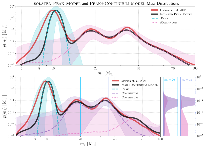
Figure 1: The astrophysical primary mass distribution inferred by the Isolated Peak Model (top) and the Peak+Continuum Model (bottom left). In both panels, the median distribution inferred by Edelman et al. (2023)is shown in red and the total inferred by this work is shown in black. The median of the subpopulation component distributions are shown in dashed lines and the shaded regions indicate the $90\%$ credible regions. The bottom right two panels show the probability density at two particular mass values, $p(m_{1}=20)$ (left) and $p(m_{1}=35)$ (right), for the posterior draws of SpinPop_A:Continuum (purple) and SpinPop_B:Continuum (pink). The subpopulation distributions are weighted by their respective branching ratios.

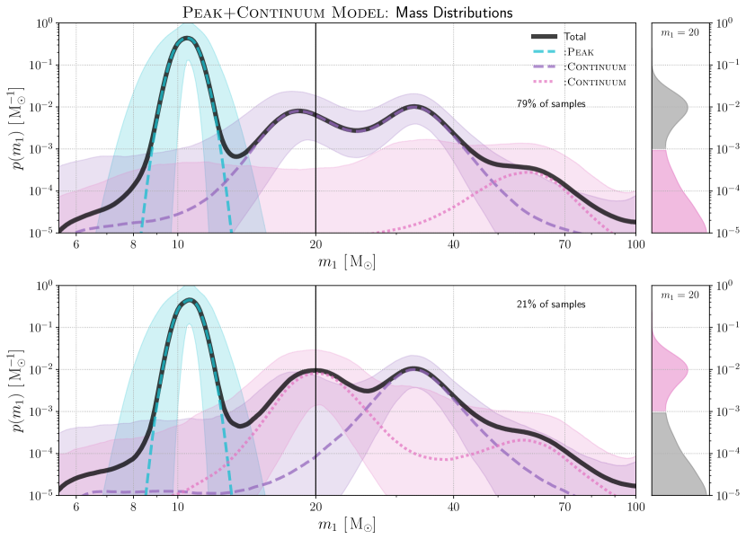
Figure 2: The astrophysical primary mass distributions inferred by the Peak+Continuum Model. The top (bottom) panel represents $79\%$ ($21\%$) of the posterior draws of Peak+Continuum Model, specifically those where $p(m_{1}=20)<10^{-3}$ ($p(m_{1}=20)>10^{-3}$) for SpinPop_B:Continuum. In both panels, the median total distribution is shown in black. The median of the subpopulation component distributions are shown in dashed lines and the shaded regions indicate the $90\%$ credible regioins. The subpopulation distributions are weighted by their respective branching ratios.

With these models and framework in hand, we infer the mass and spin distributions with the most recent LVK catalog of gravitational wave observations, GWTC-3 (The LIGO Scientific Collaboration et al., 2021a). We perform the same BBH threshold cuts on the catalog done by the LVK’s accompanying population analysis Abbott et al. (2021d), but additionally choose to remove GW190814, as it is likely an outlier of the total BBH population and is not very well understood (Abbott et al., 2021d; The LIGO Scientific Collaboration et al., 2021c; Essick et al., 2022). For the remaining 69 BBH mergers, we follow what was done in The LIGO Scientific Collaboration et al. (2021a): for events included in GWTC-1 (Abbott et al., 2019b), we use the published samples that equally weight samples from analyses with the IMRPhenomPv2 (Hannam et al., 2014) and SEOBNRv3 (Pan et al., 2014; Taracchini et al., 2014) waveforms; for the events from GWTC-2 (Abbott et al., 2021b), we use samples that equally weight all available analyses using higher-order mode waveforms (PrecessingIMRPHM); finally, for new events reported in GWTC-2.1 and GWTC-3 (The LIGO Scientific Collaboration et al., 2021a, d), we use combined samples, equally weighted, from analyses with the IMRPhenomXPHM (Pratten et al., 2021) and the SEOBNRv4PHM (Ossokine et al., 2020) waveform models.

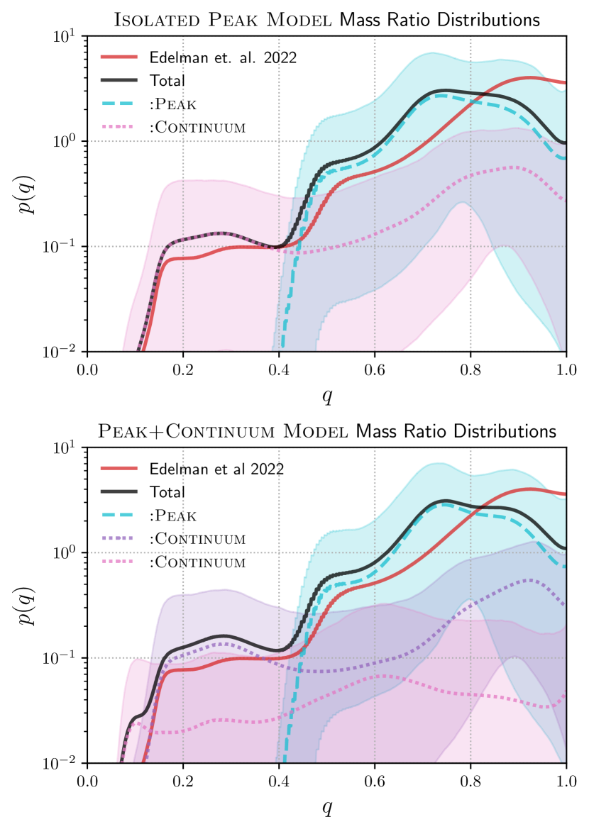
Figure 3: The astrophysical mass ratio distributions inferred by the Isolated Peak Model (top) and the Peak+Continuum Model (bottom). In both panels, the median distribution inferred by Edelman et al. (2023)is shown in red and the total inferred by this work is shown in black. The median of the subpopulation component distributions are shown in dashed lines and the shaded regions indicate the $90\%$ credible regions. The subpopulation distributions are weighted by their respective branching ratios.

3.1 BBH Mass and Spin Distributions

Figure 1 shows the primary mass distributions of the Isolated Peak Model, as well as the total primary mass distribution inferred by Edelman et al. (2023) for comparison. As seen in Figure 1, the total BBH primary mass distribution of the Isolated Peak Model is statistically consistent with that inferred by Edelman et al. (2023). Inspecting the subpopulations, SpinPop_A:Peak and SpinPop_B:Continuum, we see that SpinPop_A:Peak identifies a peak in the primary mass spectrum near $10{\,\rm M}_{\odot}$ while SpinPop_B:Continuum describes the rest of the spectrum above the peak. Interestingly, even though the $35{\,\rm M}_{\odot}$ peak was the first observed departure from power law-like behavior in the mass spectrum (with GWTC-2), the spin characteristics of binaries in this peak are perhaps not as distinct as those in the $10{\,\rm M}_{\odot}$ peak for SpinPop_A:Peak to isolate it from the rest of the population. As we will discuss later, this does not necessarily imply that binaries in the $35{\,\rm M}_{\odot}$ peak do not have spin characteristics distinct from other parts of the mass spectrum. Figure 3 shows the mass ratio distributions of the Isolated Peak Model and Peak+Continuum Model. Though uncertainties are large, the distributions across subpopulations have consistent features (the sharp fall-off of SpinPop_A:Peak near $q=0.4$ in both models is due to the fixed minimum mass $m_{\text{min}}=5{\,\rm M}_{\odot}$, and events in SpinPop_A:Peak are $\lesssim 10{\,\rm M}_{\odot}$). The total mass ratio distributions for both models are consistent with the total inferred by Edelman et al. (2023).

Figure 4 shows the inferred spin magnitude and tilt distributions for the two components. We see that the events categorized in SpinPop_A prefer lower spins than those in SpinPop_B and have a stronger preference for alignment than their higher mass counterparts. Specifically, the tilt distribution of SpinPop_A peaks at $\cos{\theta}=$ ${0.53^{+0.47}_{-0.95}}$ and has a fraction of negative tilts $f_{\cos{\theta}<0}=$ ${0.35^{+0.16}_{-0.13}}$ while SpinPop_B’s spin tilt distribution peaks at $\cos{\theta}=$ ${0.19^{+0.81}_{-0.73}}$, with $f_{\cos{\theta}<0}=$ ${0.43^{+0.13}_{-0.12}}$. Given that isolated binary evolution is theorized to produce a population of BBH’s with similar mass and spin characteristics, SpinPop_A:Peak is consistent with a subpopulation of BBH’s formed through isolated binary evolution. Due to the large uncertainties in the measured spin parameters, it’s important to note that these spin inferences only hint at unique features of a given subset of events. To confidently associate these BBH’s with the field formation channel, more observations are needed.

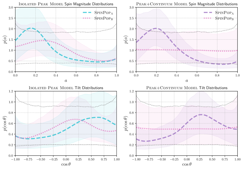
Figure 4: The spin magnitude and tilt distributions inferred by the Isolated Peak Model (top left and bottom left) and the Peak+Continuum Model (top right and bottom right). In each panel, the medians of the subpopulation component distributions are shown in dashed lines and the shaded regions indicate the $90\%$ credible regions. The dashed gray lines show the $90\%$ credible bounds of the B-Spline models’ prior predictive distributions. The subpopulation distributions are not weighted by their respective branching ratios.

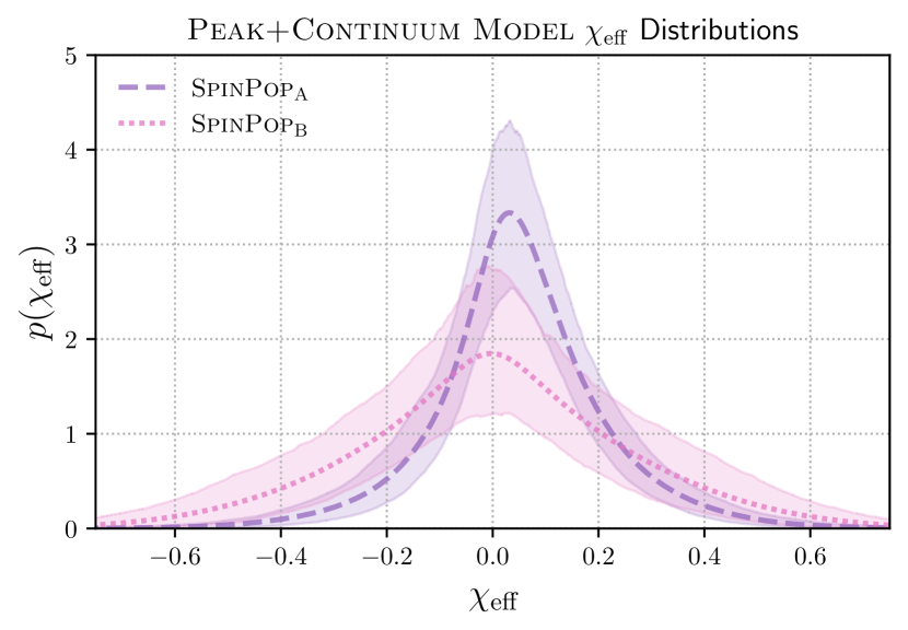
Figure 5: The effective spin distribution inferred by the Peak+Continuum Model. The medians of the subpopulation component distributions are shown in dashed lines and the shaded regions indicate the $90\%$ credible regions. The subpopulation distributions are not weighted by their respective branching ratios.

The need for more data is even more apparent when we consider the rest of the BBH population and the results of the Peak+Continuum Model. The primary mass distributions of the Peak+Continuum Model are shown in the bottom panel of Figure 1, again plotted alongside the total distribution inferred by Edelman et al. (2023). From this figure, we see that the events in the $\sim 15-50{\,\rm M}_{\odot}$ range are described by SpinPop_A:Continuum, which is the component that shares spin properties with SpinPop_A:Peak. The tail end of the mass spectrum is then picked up by SpinPop_B:Continuum. Looking to Figure 4, the top right panel shows that the spin magnitude distribution of SpinPop_A resembles that of SpinPop_A from the Isolated Peak Model, while the distribution of SpinPop_B is completely uninformed. In the bottom right panel, the tilt distribution of SpinPop_A in the Peak+Continuum Model also shares similarities with that of SpinPop_A in the Isolated Peak Model, and again SpinPop_B possess an uninformed distribution. Figure 5 shows the effective spin distributions of the Peak+Continuum Model, where we see the SpinPop_A distribution exhibits an effective spin distribution peaking at positive values while the SpinPop_B effective spin distribution looks more isotropic, and is symmetric about $\chi_{\mathrm{eff}}=0$. Our findings are consistent with previous studies (The LIGO Scientific Collaboration et al., 2021c; Hoy et al., 2022) that have found that the spin magnitudes of BBHs with primary masses $\gtrsim 45-50{\,\rm M}_{\odot}$ are more poorly constrained than lower mass binaries, with a tendency toward larger spin magnitudes.

Given these observations, it may be tempting to claim that all the mid-mass events categorized in SpinPop_A:Continuum have spin properties consistent with SpinPop_A:Peak and therefore may be the product of the same formation mechanism as SpinPop_A:Peak; however, a closer look at the results shows there is some uncertainty in how the $20{\,\rm M}_{\odot}$ peak is categorized. Rather than looking only at the band indicating the central 90% credible interval of the primary mass probability density, if for SpinPop_B:Continuum we look at the posterior distribution of the probability density at a slice $m_{1}=20{\,\rm M}_{\odot}$, we find the population constraints to be bimodal. Making a cut through the posterior draws at the inflection point between the two modes, we recreate Figure 1 in Figure 2 but for these two different regions of (hyper-)parameter space. The top panel of 2 represents $\sim 80\%$ of the posterior draws while the bottom represents $\sim 20\%$. We see that while most of the time, the events near $20{\,\rm M}_{\odot}$ are categorized with SpinPop_A:Continuum and therefore associated with the $10{\,\rm M}_{\odot}$ peak and $35{\,\rm M}_{\odot}$ peak, there is a small probability that they are actually associated with the highest mass events and therefore could be consistent with an isotropic spin distribution. Importantly, SpinPop_A:Continuum rarely picks up the high mass tail of the mass spectrum, which marks those events as distinct from the $10{\,\rm M}_{\odot}$ and $35{\,\rm M}_{\odot}$ peaks.

The location of SpinPop_A:Peak in the mass spectrum is robust against our choice of model. We implemented a number of different parametric subpopulations alongside SpinPop_A:Peak in our preliminary investigations and still found the location of SpinPop_A:Peak to be $10{\,\rm M}_{\odot}$ in primary mass. We chose to relax our assumptions on each subpopulation, ultimately opting for non-parametric B-Splines for the mass distributions of SpinPop_A:Continuum and SpinPop_B:Continuum and all the spin distributions in order to keep any model biases in our results minimal. A recent work, Li et al. (2023), conducted a similar study that inferred the existence of two subpopulations in the GWTC-3 catalog data, one with masses $\lesssim 40{\,\rm M}_{\odot}$ and low spin magnitude and the other with masses in the range $20-90{\,\rm M}_{\odot}$, isotropic spins, and a spin magnitude distribution peaking at $a_{\text{peak}}\sim 0.8$. These results are not consistent with the mass and spin distributions we infer; however, model biases may be responsible for the differences in our results. In our preliminary investigations using parametric spin models, such as truncated Gaussians, we recovered similar spin distributions as their high-spin group (HSG). We noticed that features in our recovered distributions, specifically the peak in the spin magnitude distribution at $\sim 0.8$, were significantly impacted by our choice of prior boundaries on the standard deviation hyper-parameter.

3.2 Astrophysical Branching Ratios and Event Categorization

Table LABEL:tab:table lists the astrophysical branching ratios and the number of events constraining each subpopulation/component of the Isolated Peak Model and Peak+Continuum Model. The branching ratio and number of events of SpinPop_A:Peak are consistent between the Isolated Peak Model and Peak+Continuum Model. Figure 6 provides a visual representation of event categorization for the Peak+Continuum Model as well as the physical properties of the subpopulations. Within SpinPop_A:Continuum, events GW190412 and GW190517_055101 are likely outliers of the subpopulation due to their visually different spin distributions. This may indicate that while our models can identify subpopulation-level features in the catalog, categorization of an individual event to a particular subpopulation does not guarantee it is truly a member of that subpopulation. GW190412 and GW190517_055101 were both detections with fairly certain spin properties. GW190412 was the first clearly unequal mass binary detection, which allowed for a measure of definitively non-zero primary spin magnitude (Zevin et al., 2020; Abbott et al., 2021e). GW190517_055101 was highlighted in the GWTC-2 catalog paper Abbott et al. (2021e) for having the highest $\chi_{\text{eff}}$ values, which can be seen in Figure 10 of Abbott et al. (2021e). The categorization of these potential outliers may have an impact on the resulting subpopulation distributions, so in future work it will be important to incorporate a method for categorizing outliers that don’t fit into any of the given subpopulations. A look at the highest mass events in Figure 6 reveals that most of them are characterized with about equal posterior odds between SpinPop_A:Continuum and SpinPop_B:Continuum. The spin distributions of these events are largely uninformed, so it is not surprising they are categorized into each component roughly equally.

Isolated Peak Model	$\lambda$	$N_{\text{events}}$	$a_{\text{peak}}$	$\cos{}(\theta)_{\text{peak}}$	$\cos{}(\theta)_{10\%}$	$\chi_{\text{eff,peak}}$
SpinPopA:Peak	${0.82^{+0.08}_{-0.16}}$	${15^{+0.0}_{-1.0}}$	${0.16^{+0.19}_{-0.16}}$	${0.53^{+0.47}_{-0.95}}$	${0.35^{+0.16}_{-0.13}}$	${0.035^{+0.046}_{-0.038}}$
SpinPopB:Continuum	${0.18^{+0.16}_{-0.08}}$	${54^{+1.0}_{-0.0}}$	${0.26^{+0.28}_{-0.26}}$	${0.19^{+0.81}_{-0.73}}$	${0.43^{+0.13}_{-0.12}}$	${0.017^{+0.044}_{-0.042}}$
Peak+Continuum Model	$\lambda$	$N_{\text{events}}$	$a_{\text{peak}}$	$\cos{}(\theta)_{\text{peak}}$	$\cos{}(\theta)_{10\%}$	$\chi_{\text{eff,peak}}$
SpinPopA:Peak	${0.81^{+0.084}_{-0.14}}$	${15^{+0.0027}_{-0.29}}$	${0.19^{+0.16}_{-0.19}}$	${0.34^{+0.66}_{-0.42}}$	${0.36^{+0.11}_{-0.1}}$	${0.031^{+0.032}_{-0.028}}$
SpinPopA:Continuum	${0.16^{+0.13}_{-0.086}}$	${46^{+6.5}_{-12}}$
SpinPopB:Continuum	${0.016^{+0.12}_{-0.013}}$	${7.8^{+12}_{-6.5}}$	${0.46^{+0.54}_{-0.46}}$	${0.03^{+0.97}_{-1.0}}$	${0.5^{+0.18}_{-0.17}}$	${{-}0.003^{+0.092}_{-0.094}}$

Table 1: The astrophysical branching ratio $\lambda$ of each subpopulation, the number of events that constrain each subpopulation $N_{\text{event}}$, and a summary of their spin distributions.

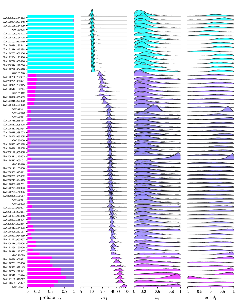
Figure 6: The left most panel shows probability of each event belonging to SpinPop_A:Peak (cyan), SpinPop_A:Continuum (purple), and SpinPop_B:Continuum (magenta). The right three panels show the population reweighed single event primary mass, spin magnitude, and spin tilt posteriors. Gray dashed lines indicate the original unweighed posteriors.

4 Astrophysical Interpretation

Spin predictions of binaries formed in the stellar field are dependent on the many physical processes that may occur prior to the stellar binary becoming a BBH. Spin magnitude of a BH can depend sensitively on the efficiency of angular momentum (AM) transport between its progenitor stellar core and envelope (Zevin & Bavera, 2022). Efficient AM transport, such as through the Taylor-Spruit magnetic dynamo (Spruit, 2002), leads to low spinning BHs (Fuller & Ma, 2019) while less efficient AM transport, such as that predicted by the shellular model (Zahn, 1992; Ekström et al., 2012; Limongi & Chieffi, 2018; Costa et al., 2019), can preserve the spin of the progenitor star. However, the effects of AM transport by these mechanisms can be obfuscated by tidal interactions between the binary components, accretion, and mass transfer, which can spin up the binary or increase AM transport efficiency, thus shedding spin. Natal supernova kicks are thought to be the leading cause of spin orbit misalignments in field binaries, while tidal forces and mass transfer tend to align BH spins with the orbital AM. As discussed in The LIGO Scientific Collaboration et al. (2021c), recent studies of BBH formation in globular cluster predict suppressed merger rates for binaries with primary BH masses $\lesssim 10{\,\rm M}_{\odot}$ (Antonini & Gieles, 2020; Rodriguez et al., 2019b; Hong et al., 2018). Therefore, BBH formation in globular clusters is unlikely to be responsible for the BBHs in the $10{\,\rm M}_{\odot}$ peak, and is most likely a subdominant formation mechanism in the catalog. While we find that the $10{\,\rm M}_{\odot}$ subpopulation is consistent with the general characteristics associated with field formation, large uncertainties in both spin measurements and predictions from population synthesis models prevent us from placing informative constraints on the formation physics. If the $10{\,\rm M}_{\odot}$ subpopulation is indeed a product of isolated binary evolution, then our inferred spin distributions hint at this channel producing binaries with low, modestly misaligned spins. This could indicate that AM transport is efficient in massive stars, as modeled by variations of the Taylor-Spruit magnetic dynamo (Belczynski et al., 2020), and that natal kicks are a common occurrence during field BBH formation.

Our results are consistent with other analyses that find the data does not require a non-spinning subpopulation (Callister et al., 2022b; Périgois et al., 2023), though is in tension with other analyses that have claimed its existence (Galaudage et al., 2021b; Roulet et al., 2021b); however, we cannot completely rule out a non-spinning population. The $35{\,\rm M}_{\odot}$ peak may also be consistent with field formation, as we infer spin properties similar to those of the $10{\,\rm M}_{\odot}$ peak. The astrophysical branching ratios we infer in the Peak+Continuum Model are consistent with the field and dynamical branching ratios inferred by Zevin et al. (2021), $[\beta_{\text{field}},\beta_{\text{dynamical}}]=[0.86^{+0.11}_{-0.36},0.14^{0.36}_{-0.11}]$, under the assumption that SpinPop_A:Peak and SpinPop_A:Continuum are consistent with field formation and SpinPop_B:Continuum is more consistent with dynamical formation.

The sharp fall-off in primary mass of SpinPop_A:Continuum in the Peak+Continuum Model could give an estimate of the lower edge of the PISN mass gap. The 99th percentile of the primary mass distribution of SpinPop_A:Continuum is $m_{1,99\%}=$ ${49^{+25}_{-8.1}}$ ${\,\rm M}_{\odot}$, which is consistent with predictions that place the lower edge of the gap between $40-70{\,\rm M}_{\odot}$ (Woosley, 2019; Farmer et al., 2019; Woosley & Heger, 2021; Edelman et al., 2021).

5 Conclusion

As the catalog of compact object mergers continues to grow, we are able to probe the physical properties of these systems with higher fidelity and uncover details in their distributions previously obscured by our lack of data. With these advancements comes the ability to piece together formation histories imprinted in the details of these distributions. Understanding the physical properties of compact binaries and their formation has implications for the broader astrophysics community such as providing constraints on stellar evolution theories and population synthesis simulations, the physics of globular clusters, the impact of stellar metallicity, neutron star equations of state, and much more.

By leveraging the hierarchical Bayesian inference toolkit, a mixture of parametric and non-parametric models, and combining information across mass and spin, we were able to identify a peak in the BBH primary mass spectrum at $m_{\text{1,peak}}=$ ${10^{+0.95}_{-0.83}}$ ${\,\rm M}_{\odot}$ that corresponds to a subpopulation of BBH’s with low spins and a moderate preference for alignment, consistent with isolated binary formation. We then extended our Isolated Peak Model to search the rest of the mass spectrum for events with similar spin characteristics to the $10{\,\rm M}_{\odot}$ subpopulation. We found that the peak in the mass spectrum near $35{\,\rm M}_{\odot}$ was consistent with the $10{\,\rm M}_{\odot}$ events. The categorization of the $20{\,\rm M}_{\odot}$ events remains unclear, since $\sim 20\%$ of posterior samples categorized the $20{\,\rm M}_{\odot}$ peak with the highest mass events. We find evidence of a distinct population at high mass whose spin properties are largely uninformed by the current catalog.

Due to the large uncertainties that are currently present in measurements of BBH properties and population synthesis models, we are unable to place strong constraints on the physics behind isolated binary evolution or (P)PISN. However, if our $10{\,\rm M}_{\odot}$ and $35{\,\rm M}_{\odot}$ subpopulations are truly products of these channels, they likely produce binaries with low spins, though the subpopulations being dominated by non-spinning BHs is not ruled out. Aligned spin systems are also not completely ruled out, but the subpopulations appear to possess modest misalignments and the apparent fall-off of the $35{\,\rm M}_{\odot}$ peak may indicate a lower bound on the PISN mass gap of ${49^{+25}_{-8.1}}$ ${\,\rm M}_{\odot}$.

The discrete latent variable framework laid out in this analysis and developed in the python library GWInferno can be used to understand the full compact binary catalog beyond identifying BBH subpopulations. Currently, the LVK categorizes mergers as binary black holes, binary neutron stars, or neutron star binary black holes a priori based on mass thresholds and tidal deformation values. Instead of categorizing merger components a priori and then fitting the mass and spin distributions of each category individually, discrete latent variables could be used to simultaneously classify merger components and infer their mass and spin distributions.

In future work, we will incorporate a method for classifying outliers to subpopulations as well as testing this framework on a simulated catalog in order to better understand how uninformed data affects our results. Repeating this analysis on the data from the next observing run – which is expected to substantially increase the current catalog size – should provide more insights with stronger constraints on subpopulation properties.

6 Acknowledgements

This material is based upon work supported by the National Science Foundation Graduate Research Fellowship under Grant No. 2236419. This research has made use of data, software and/or web tools obtained from the Gravitational Wave Open Science Center (https://www.gw-openscience.org/), a service of LIGO Laboratory, the LIGO Scientific Collaboration and the Virgo Collaboration. The authors are grateful for computational resources provided by the LIGO Laboratory and supported by National Science Foundation Grants PHY-0757058 and PHY-0823459. This work benefited from access to the University of Oregon high performance computer, Talapas. This material is based upon work supported in part by the National Science Foundation under Grant PHY-2146528 and work supported by NSF’s LIGO Laboratory which is a major facility fully funded by the National Science Foundation.

References

- Abbott et al. (2016) Abbott, B. P., Abbott, R., Abbott, T. D., et al. 2016, Phys. Rev. Lett., 116, 061102, doi: 10.1103/PhysRevLett.116.061102
- Abbott et al. (2019a) —. 2019a, Physical Review X, 9, 031040, doi: 10.1103/PhysRevX.9.031040
- Abbott et al. (2019b) —. 2019b, ApJ, 882, L24, doi: 10.3847/2041-8213/ab3800
- Abbott et al. (2019c) —. 2019c, ApJ, 882, L24, doi: 10.3847/2041-8213/ab3800
- Abbott et al. (2021a) Abbott, R., Abbott, T. D., Abraham, S., et al. 2021a, Physical Review X, 11, 021053, doi: 10.1103/PhysRevX.11.021053
- Abbott et al. (2021b) —. 2021b, ApJ, 913, L7, doi: 10.3847/2041-8213/abe949
- Abbott et al. (2021c) —. 2021c, ApJ, 913, L7, doi: 10.3847/2041-8213/abe949
- Abbott et al. (2021d) —. 2021d, ApJ, 913, L7, doi: 10.3847/2041-8213/abe949
- Abbott et al. (2021e) —. 2021e, Physical Review X, 11, 021053, doi: 10.1103/PhysRevX.11.021053
- Acernese et al. (2015) Acernese, F., Agathos, M., Agatsuma, K., et al. 2015, Classical and Quantum Gravity, 32, 024001, doi: 10.1088/0264-9381/32/2/024001
- Akutsu et al. (2021) Akutsu, T., Ando, M., Arai, K., et al. 2021, Progress of Theoretical and Experimental Physics, 2021, 05A102, doi: 10.1093/ptep/ptab018
- Antonini & Gieles (2020) Antonini, F., & Gieles, M. 2020, Phys. Rev. D, 102, 123016, doi: 10.1103/PhysRevD.102.123016
- Arca Sedda et al. (2020) Arca Sedda, M., Mapelli, M., Spera, M., Benacquista, M., & Giacobbo, N. 2020, ApJ, 894, 133, doi: 10.3847/1538-4357/ab88b2
- Astropy Collaboration et al. (2013) Astropy Collaboration, Robitaille, T. P., Tollerud, E. J., et al. 2013, A&A, 558, A33, doi: 10.1051/0004-6361/201322068
- Astropy Collaboration et al. (2018) Astropy Collaboration, Price-Whelan, A. M., Sipőcz, B. M., et al. 2018, AJ, 156, 123, doi: 10.3847/1538-3881/aabc4f
- Astropy Collaboration et al. (2022) Astropy Collaboration, Price-Whelan, A. M., Lim, P. L., et al. 2022, ApJ, 935, 167, doi: 10.3847/1538-4357/ac7c74
- Bavera et al. (2020) Bavera, S. S., Fragos, T., Qin, Y., et al. 2020, A&A, 635, A97, doi: 10.1051/0004-6361/201936204
- Belczynski et al. (2016) Belczynski, K., Holz, D. E., Bulik, T., & O’Shaughnessy, R. 2016, Nature, 534, 512, doi: 10.1038/nature18322
- Belczynski et al. (2020) Belczynski, K., Klencki, J., Fields, C. E., et al. 2020, A&A, 636, A104, doi: 10.1051/0004-6361/201936528
- Bingham et al. (2018) Bingham, E., Chen, J. P., Jankowiak, M., et al. 2018, arXiv e-prints, arXiv:1810.09538. https://arxiv.org/abs/1810.09538
- Biscoveanu et al. (2022) Biscoveanu, S., Callister, T. A., Haster, C.-J., et al. 2022, ApJ, 932, L19, doi: 10.3847/2041-8213/ac71a8
- Bradbury et al. (2018) Bradbury, J., Frostig, R., Hawkins, P., et al. 2018, JAX: composable transformations of Python+NumPy programs, 0.3.13. http://github.com/google/jax
- Callister et al. (2021a) Callister, T. A., Farr, W. M., & Renzo, M. 2021a, ApJ, 920, 157, doi: 10.3847/1538-4357/ac1347
- Callister et al. (2021b) Callister, T. A., Haster, C.-J., Ng, K. K. Y., Vitale, S., & Farr, W. M. 2021b, ApJ, 922, L5, doi: 10.3847/2041-8213/ac2ccc
- Callister et al. (2022a) Callister, T. A., Miller, S. J., Chatziioannou, K., & Farr, W. M. 2022a, ApJ, 937, L13, doi: 10.3847/2041-8213/ac847e
- Callister et al. (2022b) —. 2022b, ApJ, 937, L13, doi: 10.3847/2041-8213/ac847e
- Costa et al. (2019) Costa, G., Girardi, L., Bressan, A., et al. 2019, MNRAS, 485, 4641, doi: 10.1093/mnras/stz728
- Dominik et al. (2013) Dominik, M., Belczynski, K., Fryer, C., et al. 2013, ApJ, 779, 72, doi: 10.1088/0004-637X/779/1/72
- Edelman et al. (2021) Edelman, B., Doctor, Z., & Farr, B. 2021, ApJ, 913, L23, doi: 10.3847/2041-8213/abfdb3
- Edelman et al. (2022) Edelman, B., Doctor, Z., Godfrey, J., & Farr, B. 2022, ApJ, 924, 101, doi: 10.3847/1538-4357/ac3667
- Edelman et al. (2023) Edelman, B., Farr, B., & Doctor, Z. 2023, ApJ, 946, 16, doi: 10.3847/1538-4357/acb5ed
- Ekström et al. (2012) Ekström, S., Georgy, C., Eggenberger, P., et al. 2012, A&A, 537, A146, doi: 10.1051/0004-6361/201117751
- Essick et al. (2022) Essick, R., Farah, A., Galaudage, S., et al. 2022, ApJ, 926, 34, doi: 10.3847/1538-4357/ac3978
- Essick & Farr (2022) Essick, R., & Farr, W. 2022, arXiv e-prints, arXiv:2204.00461, doi: 10.48550/arXiv.2204.00461
- Farah et al. (2023) Farah, A. M., Edelman, B., Zevin, M., et al. 2023, arXiv e-prints, arXiv:2301.00834, doi: 10.48550/arXiv.2301.00834
- Farmer et al. (2019) Farmer, R., Renzo, M., de Mink, S. E., Marchant, P., & Justham, S. 2019, ApJ, 887, 53, doi: 10.3847/1538-4357/ab518b
- Farr et al. (2018) Farr, B., Holz, D. E., & Farr, W. M. 2018, ApJ, 854, L9, doi: 10.3847/2041-8213/aaaa64
- Farr (2019) Farr, W. M. 2019, Research Notes of the American Astronomical Society, 3, 66, doi: 10.3847/2515-5172/ab1d5f
- Farr et al. (2015) Farr, W. M., Gair, J. R., Mandel, I., & Cutler, C. 2015, Phys. Rev. D, 91, 023005, doi: 10.1103/PhysRevD.91.023005
- Farr et al. (2017) Farr, W. M., Stevenson, S., Miller, M. C., et al. 2017, Nature, 548, 426, doi: 10.1038/nature23453
- Fishbach & Holz (2017) Fishbach, M., & Holz, D. E. 2017, ApJ, 851, L25, doi: 10.3847/2041-8213/aa9bf6
- Fishbach et al. (2022) Fishbach, M., Kimball, C., & Kalogera, V. 2022, ApJ, 935, L26, doi: 10.3847/2041-8213/ac86c4
- Fishbach et al. (2021) Fishbach, M., Doctor, Z., Callister, T., et al. 2021, ApJ, 912, 98, doi: 10.3847/1538-4357/abee11
- Fuller & Ma (2019) Fuller, J., & Ma, L. 2019, ApJ, 881, L1, doi: 10.3847/2041-8213/ab339b
- Galaudage et al. (2021a) Galaudage, S., Talbot, C., Nagar, T., et al. 2021a, ApJ, 921, L15, doi: 10.3847/2041-8213/ac2f3c
- Galaudage et al. (2021b) —. 2021b, ApJ, 921, L15, doi: 10.3847/2041-8213/ac2f3c
- Giacobbo & Mapelli (2018) Giacobbo, N., & Mapelli, M. 2018, MNRAS, 480, 2011, doi: 10.1093/mnras/sty1999
- Hannam et al. (2014) Hannam, M., Schmidt, P., Bohé, A., et al. 2014, Phys. Rev. Lett., 113, 151101, doi: 10.1103/PhysRevLett.113.151101
- Harris et al. (2020) Harris, C. R., Millman, K. J., van der Walt, S. J., et al. 2020, Nature, 585, 357, doi: 10.1038/s41586-020-2649-2
- Hoffman & Gelman (2011) Hoffman, M. D., & Gelman, A. 2011, arXiv e-prints, arXiv:1111.4246. https://arxiv.org/abs/1111.4246
- Hogg (1999) Hogg, D. W. 1999, arXiv e-prints, astro. https://arxiv.org/abs/astro-ph/9905116
- Hong et al. (2018) Hong, J., Vesperini, E., Askar, A., et al. 2018, MNRAS, 480, 5645, doi: 10.1093/mnras/sty2211
- Hoy et al. (2022) Hoy, C., Fairhurst, S., Hannam, M., & Tiwari, V. 2022, ApJ, 928, 75, doi: 10.3847/1538-4357/ac54a3
- Hunter (2007) Hunter, J. D. 2007, Computing in Science and Engineering, 9, 90, doi: 10.1109/MCSE.2007.55
- Li et al. (2023) Li, Y.-J., Wang, Y.-Z., Tang, S.-P., & Fan, Y.-Z. 2023, arXiv e-prints, arXiv:2303.02973, doi: 10.48550/arXiv.2303.02973
- LIGO Scientific Collaboration et al. (2015) LIGO Scientific Collaboration, Aasi, J., Abbott, B. P., et al. 2015, Classical and Quantum Gravity, 32, 074001, doi: 10.1088/0264-9381/32/7/074001
- Limongi & Chieffi (2018) Limongi, M., & Chieffi, A. 2018, ApJS, 237, 13, doi: 10.3847/1538-4365/aacb24
- Liu (1996) Liu, J. S. 1996, Biometrika, 83, 681
- Loredo (2004) Loredo, T. J. 2004, in American Institute of Physics Conference Series, Vol. 735, Bayesian Inference and Maximum Entropy Methods in Science and Engineering: 24th International Workshop on Bayesian Inference and Maximum Entropy Methods in Science and Engineering, ed. R. Fischer, R. Preuss, & U. V. Toussaint, 195–206, doi: 10.1063/1.1835214
- Luger et al. (2021) Luger, R., Bedell, M., Foreman-Mackey, D., et al. 2021, arXiv e-prints, arXiv:2110.06271. https://arxiv.org/abs/2110.06271
- Mahapatra et al. (2022) Mahapatra, P., Gupta, A., Favata, M., Arun, K. G., & Sathyaprakash, B. S. 2022, arXiv e-prints, arXiv:2209.05766, doi: 10.48550/arXiv.2209.05766
- Mandel & Broekgaarden (2022) Mandel, I., & Broekgaarden, F. S. 2022, Living Reviews in Relativity, 25, 1, doi: 10.1007/s41114-021-00034-3
- Mandel et al. (2019) Mandel, I., Farr, W. M., & Gair, J. R. 2019, MNRAS, 486, 1086, doi: 10.1093/mnras/stz896
- Ossokine et al. (2020) Ossokine, S., Buonanno, A., Marsat, S., et al. 2020, Phys. Rev. D, 102, 044055, doi: 10.1103/PhysRevD.102.044055
- Pan et al. (2014) Pan, Y., Buonanno, A., Taracchini, A., et al. 2014, Phys. Rev. D, 89, 084006, doi: 10.1103/PhysRevD.89.084006
- Périgois et al. (2023) Périgois, C., Mapelli, M., Santoliquido, F., Bouffanais, Y., & Rufolo, R. 2023, arXiv e-prints, arXiv:2301.01312, doi: 10.48550/arXiv.2301.01312
- Phan et al. (2019) Phan, D., Pradhan, N., & Jankowiak, M. 2019, arXiv e-prints, arXiv:1912.11554. https://arxiv.org/abs/1912.11554
- Pratten et al. (2021) Pratten, G., García-Quirós, C., Colleoni, M., et al. 2021, Phys. Rev. D, 103, 104056, doi: 10.1103/PhysRevD.103.104056
- Rodriguez et al. (2016a) Rodriguez, C. L., Chatterjee, S., & Rasio, F. A. 2016a, Phys. Rev. D, 93, 084029, doi: 10.1103/PhysRevD.93.084029
- Rodriguez et al. (2019a) Rodriguez, C. L., Zevin, M., Amaro-Seoane, P., et al. 2019a, Phys. Rev. D, 100, 043027, doi: 10.1103/PhysRevD.100.043027
- Rodriguez et al. (2019b) —. 2019b, Phys. Rev. D, 100, 043027, doi: 10.1103/PhysRevD.100.043027
- Rodriguez et al. (2016b) Rodriguez, C. L., Zevin, M., Pankow, C., Kalogera, V., & Rasio, F. A. 2016b, ApJ, 832, L2, doi: 10.3847/2041-8205/832/1/L2
- Roulet et al. (2021a) Roulet, J., Chia, H. S., Olsen, S., et al. 2021a, Phys. Rev. D, 104, 083010, doi: 10.1103/PhysRevD.104.083010
- Roulet et al. (2021b) —. 2021b, Phys. Rev. D, 104, 083010, doi: 10.1103/PhysRevD.104.083010
- Spruit (2002) Spruit, H. C. 2002, A&A, 381, 923, doi: 10.1051/0004-6361:20011465
- Stevenson et al. (2017) Stevenson, S., Berry, C. P. L., & Mandel, I. 2017, MNRAS, 471, 2801, doi: 10.1093/mnras/stx1764
- Stevenson et al. (2015) Stevenson, S., Ohme, F., & Fairhurst, S. 2015, ApJ, 810, 58, doi: 10.1088/0004-637X/810/1/58
- Talbot & Thrane (2018) Talbot, C., & Thrane, E. 2018, ApJ, 856, 173, doi: 10.3847/1538-4357/aab34c
- Taracchini et al. (2014) Taracchini, A., Buonanno, A., Pan, Y., et al. 2014, Phys. Rev. D, 89, 061502, doi: 10.1103/PhysRevD.89.061502
- The LIGO Scientific Collaboration et al. (2021a) The LIGO Scientific Collaboration, the Virgo Collaboration, the KAGRA Collaboration, et al. 2021a, arXiv e-prints, arXiv:2111.03606. https://arxiv.org/abs/2111.03606
- The LIGO Scientific Collaboration et al. (2021b) —. 2021b, arXiv e-prints, arXiv:2111.03634. https://arxiv.org/abs/2111.03634
- The LIGO Scientific Collaboration et al. (2021c) —. 2021c, arXiv e-prints, arXiv:2111.03634. https://arxiv.org/abs/2111.03634
- The LIGO Scientific Collaboration et al. (2021d) The LIGO Scientific Collaboration, the Virgo Collaboration, Abbott, R., et al. 2021d, arXiv e-prints, arXiv:2108.01045, doi: 10.48550/arXiv.2108.01045
- Tiwari (2018) Tiwari, V. 2018, Classical and Quantum Gravity, 35, 145009, doi: 10.1088/1361-6382/aac89d
- Tiwari (2022) —. 2022, ApJ, 928, 155, doi: 10.3847/1538-4357/ac589a
- Tiwari & Fairhurst (2021) Tiwari, V., & Fairhurst, S. 2021, ApJ, 913, L19, doi: 10.3847/2041-8213/abfbe7
- Tong et al. (2022) Tong, H., Galaudage, S., & Thrane, E. 2022, arXiv e-prints, arXiv:2209.02206. https://arxiv.org/abs/2209.02206
- van Son et al. (2022) van Son, L. A. C., de Mink, S. E., Callister, T., et al. 2022, ApJ, 931, 17, doi: 10.3847/1538-4357/ac64a3
- Virtanen et al. (2020) Virtanen, P., Gommers, R., Oliphant, T. E., et al. 2020, Nature Methods, 17, 261, doi: 10.1038/s41592-019-0686-2
- Vitale et al. (2022a) Vitale, S., Biscoveanu, S., & Talbot, C. 2022a, A&A, 668, L2, doi: 10.1051/0004-6361/202245084
- Vitale et al. (2022b) Vitale, S., Gerosa, D., Farr, W. M., & Taylor, S. R. 2022b, in Handbook of Gravitational Wave Astronomy. Edited by C. Bambi, 45, doi: 10.1007/978-981-15-4702-7_45-1
- Vitale et al. (2017) Vitale, S., Lynch, R., Sturani, R., & Graff, P. 2017, Classical and Quantum Gravity, 34, 03LT01, doi: 10.1088/1361-6382/aa552e
- Wang et al. (2022) Wang, Y.-Z., Li, Y.-J., Vink, J. S., et al. 2022, ApJ, 941, L39, doi: 10.3847/2041-8213/aca89f
- Woosley (2019) Woosley, S. E. 2019, ApJ, 878, 49, doi: 10.3847/1538-4357/ab1b41
- Woosley & Heger (2021) Woosley, S. E., & Heger, A. 2021, ApJ, 912, L31, doi: 10.3847/2041-8213/abf2c4
- Zahn (1992) Zahn, J. P. 1992, A&A, 265, 115
- Zevin & Bavera (2022) Zevin, M., & Bavera, S. S. 2022, ApJ, 933, 86, doi: 10.3847/1538-4357/ac6f5d
- Zevin et al. (2020) Zevin, M., Berry, C. P. L., Coughlin, S., Chatziioannou, K., & Vitale, S. 2020, ApJ, 899, L17, doi: 10.3847/2041-8213/aba8ef
- Zevin et al. (2017) Zevin, M., Pankow, C., Rodriguez, C. L., et al. 2017, ApJ, 846, 82, doi: 10.3847/1538-4357/aa8408
- Zevin et al. (2021) Zevin, M., Bavera, S. S., Berry, C. P. L., et al. 2021, ApJ, 910, 152, doi: 10.3847/1538-4357/abe40e