On the primordial black hole formation in hybrid inflation

Abstract

We revisit the scenario of primordial black hole (PBH) formation from large curvature perturbations generated during the waterfall phase transition in hybrid inflation models. In a minimal setup considered in the literature, the mass and abundance of PBHs are correlated and astrophysical size PBHs tend to be overproduced. This is because a longer length scale for curvature perturbations (or a larger PBH mass) requires a longer waterfall regime with a flatter potential, which results in overproduction of curvature perturbations. However, in this paper, we discuss that the higher-dimensional terms for the inflaton potential affect the dynamics during the waterfall phase transition and show that astrophysical size PHBs of the order of $10^{17\text{--}23}\,{\rm g}$ (which can explain the whole dark matter) can form in some parameter space consistently with any existing constraints. The scenario can be tested by observing the induced gravitational waves from scalar perturbations by future gravitational wave experiments, such as LISA.

I Introduction

The seeds of the structure of the Universe can be generated by quantum fluctuations of inflatons or curvatons during inflation. The amplitude of curvature perturbations is of the order of $10^{-5}$ at the cosmic microwave background (CMB) scale [1], whereas larger curvature perturbations may be generated at a smaller scale [2, 3, 4, 5, 6, 7]. In fact, observations of supermassive black hole (BH) [8, 9] and BH merger events by gravitational wave detectors [10, 11] imply the existence of primordial black holes that are generated via the collapse of overdense regions [12, 13, 14]. The PBH is also a candidate for dark matter (DM) [25] if its mass is within $10^{17\text{--}23}\ {\rm g}$ (see, e.g., Refs. [26, 27, 28]). Such large curvature perturbations can be generated if the inflaton or a spectator field goes through a very flat potential during inflation (see also Ref. [29] for a recent review of PBHs).

One of the simplest examples to generate large curvature perturbations is the hybrid inflation model, where inflation ends by a waterfall (second-order) phase transition [30]. The waterfall field can have a flat potential to generate large curvature perturbations [50, 51, 52]. Since the waterfall phase transition happens at the last stage of inflation, this results in large curvature perturbations at relatively small scales. Although one can make its scale larger by flattening the potential of the waterfall field, the amplitude of curvature perturbations then becomes too large. PBH mass and abundance are correlated in the minimal setup, which results in an overproduction of astrophysical size PBHs. This naive picture is actually confirmed by analytical calculation and numerical calculations in the stochastic formalism [53, 54].

In this paper, we point out that PBHs with an astrophysical size can be generated in a simple hybrid inflation model, by demonstrating that the quadratic and cubic terms for the inflaton potential affect curvature perturbations, which are omitted in the literature. In particular, the degeneracy between the PBH mass and its abundance can be removed by those effects and the peak amplitude of curvature perturbations can be reduced by tuning parameters. We discuss how much tuning is required to predict the desired amount of PBHs. Moreover, the spectral index of curvature perturbations at the CMB scale can be consistent with observations.

The organization of this paper is as follows. In Sec. II, we briefly review the analytic calculation for curvature perturbations, following Ref. [53] and clarify that the resulting spectrum has degeneracy between its peak amplitude and corresponding wavenumber if we omit quadratic and cubic terms for the inflaton potential. In Sec. III, we take into account quadratic and cubic terms for the inflaton potential and show that the degeneracy can be resolved by those effects. In Sec. III.4, we solve the classical equation of motion numerically and search parameter space that predicts a desired amplitude of curvature perturbations. We then consider PBH formation in Sec. IV and show that PBHs with mass $10^{17\text{--}23}\ {\rm g}$ can be generated consistently with all existing constraints. We also show that observable gravitational waves are generated from the second-order curvature perturbations. Sec. V is devoted to discussion and conclusions.

II Hybrid inflation model

We consider the hybrid inflation model [50, 51, 52, 53, 54]

$$V(\phi,\psi)=\Lambda^{4}\left[\pqty{1-\frac{\psi^{2}}{M^{2}}}^{2}+2\frac{\phi^{2}\psi^{2}}{\phi_{\mathrm{c}}^{2}M^{2}}+V(\phi)\right]\,,$$ (1)

where $\phi$ is an inflaton and $\psi$ is a waterfall field. We are interested in the dynamics of fields around the waterfall phase transition, where curvature perturbations are generated for the scales of interest. The inflaton potential $V(\phi)$ is expanded around the critical point $\phi_{\mathrm{c}}$ as

$$V(\phi)=\frac{\phi-\phi_{\mathrm{c}}}{\mu_{1}}-\frac{(\phi-\phi_{\mathrm{c}})^{2}}{\mu_{2}^{2}}+\frac{(\phi-\phi_{\mathrm{c}})^{3}}{\mu_{3}^{3}}\,,$$ (2)

where $\Lambda$, $M$, $\phi_{\mathrm{c}}$, $\mu_{1}$, $\mu_{2}$, and $\mu_{3}$ are dimensionful parameters. The curvature along with the waterfall direction changes its sign when the inflaton $\phi$ reaches the critical point. We denote the time at which $\phi=\phi_{\mathrm{c}}$ as the waterfall phase transition. The Hubble parameter during inflation is $H_{\rm inf}^{2}\simeq\Lambda^{4}/(3M_{\mathrm{Pl}}^{2})$. We extend the model in Refs. [53, 54] by introducing the cubic potential in $V(\phi)$. We will see that the cubic term plays an important role to obtain a desired amplitude of curvature perturbations as well as the observed spectral index.

In this section, we review the calculation for curvature perturbations generated from waterfall fields by an analytic method used in Ref. [53], omitting quadratic and cubic terms in the inflaton potential. In the next section, we include the effect of those terms.

II.1 Spectrum at the CMB scale

We first analyse the dynamics of inflaton before the waterfall phase transition, where $\phi>\phi_{\mathrm{c}}$. In this regime, we can solve the equation of motion for $\phi$ by approximating $\psi\simeq 0$.

We want to calculate the spectral index and amplitude of curvature perturbations at the CMB scale. We denote the backward e-folding number at the CMB scale and the one at the waterfall phase transition as $\mathcal{N}_{*}$ and $\mathcal{N}_{\mathrm{c}}$, respectively. The observed amplitude of curvature perturbations at the pivot scale is given by

$${\cal P}_{\mathcal{R}}(k_{*})\simeq 2.1\times 10^{-9}\,,$$ (3)

where $k_{*}$ ($=0.05\,{\rm Mpc}^{-1}$) represents the wavenumber at the pivot scale [1]. These perturbations exit the horizon before the waterfall phase transition, and should come from the fluctuation of the inflaton $\phi$. Its amplitude is calculated from

$${\cal P}_{\mathcal{R}}=\frac{H_{\rm inf}^{2}}{8\pi^{2}\epsilon M_{\mathrm{Pl}}^{2}}\,,$$ (4)

where

$$\epsilon=\frac{1}{2}\left(M_{\mathrm{Pl}}\frac{V_{\phi}}{V}\right)^{2}\simeq\frac{M_{\mathrm{Pl}}^{2}}{2\mu_{1}^{2}}\,.$$ (5)

From Eq. (3), we require

$$\Lambda\simeq 1.7\times 10^{14}\ {\rm GeV}\left(\frac{\mu_{1}}{10^{5}M_{\mathrm{Pl}}}\right)^{-1/2}\,,$$ (6)

or

$$H_{\rm inf}\simeq 7.0\times 10^{9}\ {\rm GeV}\left(\frac{\mu_{1}}{10^{5}M_{\mathrm{Pl}}}\right)^{-1}\,.$$ (7)

The e-folding number at the pivot scale is given by

$$\mathcal{N}_{*} \simeq 51.5+\frac{1}{2}\ln\left(\frac{H_{\rm inf}}{7\times 10^{9}\ {\rm GeV}}\right)+\frac{1}{6}\ln\left(\frac{H_{\rm RH}}{H_{\rm inf}}\right)\,,$$ (8)

where $H_{\rm RH}$ represents the Hubble parameter at the completion of reheating.

The spectral index is given by

$$n_{\mathrm{s}} =1+\evaluated{2M_{\mathrm{Pl}}^{2}\frac{V_{\phi\phi}}{V}}_{k_{*}}\simeq 1-4\frac{M_{\mathrm{Pl}}^{2}}{\mu_{2}^{2}}\,,$$ (9)

where we neglected the contribution of $\epsilon$ compared to that of $V_{\phi\phi}$ and $\phi_{*}$ represents the field value of $\phi$ at $\mathcal{N}=\mathcal{N}_{*}$.

II.2 Stochastic effect around the waterfall phase transition

Around the critical point $\phi=\phi_{\mathrm{c}}$, the curvature of the potential along with $\psi$ direction is so small that its quantum fluctuations efficiently grow with time. It obeys the slow-roll Langevin equation (see Refs. [55, 56, 57, 58, 59, 60, 61, 62, 63, 64] for the first papers on the subject)

$$\partial_{N}\psi=-M_{\mathrm{Pl}}^{2}\frac{V_{\psi}}{V}+\frac{1}{2\pi}\sqrt{\frac{V}{3M_{\mathrm{Pl}}^{2}}}\xi(N)\,,$$ (10)

where $N$ is the forward e-folding number as the time variable and $\xi$ is the independent noise $\braket{\xi(N)\xi(N^{\prime})}=\delta(N-N^{\prime})$. We can neglect the noise term for the inflaton $\phi$ around the waterfall phase transition for our purpose.

The noise term for $\psi$ is important at a time around and before the waterfall phase transition but can be negligible at a later time. We divide the dynamical regime into two phases: the stochastic phase and classical phase [53]. Initially, the noise term dominates $\psi$’s dynamics. This sets the initial condition for the classical phase, where the classical equation of motion (i.e., the first term in the right-hand side in Eq. (10)) dominates the dynamics. We solve the dynamics of $\psi$ and $\phi$, and calculate the curvature perturbations by the $\delta\mathcal{N}$ formalism [66, 67, 68, 69, 70].

We denote the forward e-folding number at the time of the waterfall phase transition (at which $\phi=\phi_{\mathrm{c}}$) as $N_{\mathrm{c}}$. Let us consider the dynamics around $N\approx N_{\mathrm{c}}$. If we neglect the stochastic noise for $\phi$, its solution is given by

$$\phi\simeq\phi_{\mathrm{c}}-\frac{M_{\mathrm{Pl}}^{2}(N-N_{\mathrm{c}})}{\mu_{1}}\,,$$ (11)

for $N\approx N_{\mathrm{c}}$. From Eq. (10), the equation of motion for $\left<\psi^{2}\right>$ is given by

$$\derivative{N}\left<\psi^{2}\right>=\left(\frac{4}{\Pi}\right)^{2}(N-N_{\mathrm{c}})\left<\psi^{2}\right>+\frac{H_{\rm inf}^{2}}{4\pi^{2}}\,,$$ (12)

where we define

$$\Pi\equiv\frac{M\sqrt{\mu_{1}\phi_{\mathrm{c}}}}{M_{\mathrm{Pl}}^{2}}\,.$$ (13)

The first term in the right-hand side represents the classical force, while the second term represents the stochastic force from the noise term. The solution to this equation can be written by the error function such as

$$\left<\psi^{2}\right>(N)=\psi_{0}^{2}\left[1+{\rm Erf}\left(\frac{2\sqrt{2}(N-N_{\mathrm{c}})}{\Pi}\right)\right]\exp\left[\frac{8(N-N_{\mathrm{c}})^{2}}{\Pi^{2}}\right]\,,$$ (14)

where ${\rm Erf}(x)\equiv(2/\sqrt{\pi})\int_{0}^{x}e^{-t^{2}}\differential{t}$ and we use $\left<\psi^{2}\right>\approx 0$ for $N\to-\infty$. The amplitude of $\left<\psi^{2}\right>$ at the waterfall phase transition ($N=N_{\mathrm{c}}$) is given by

$$\psi_{0}^{2}=\frac{\Lambda^{4}\Pi}{48\sqrt{2\pi^{3}}M_{\mathrm{Pl}}^{2}}\,,$$ (15)

where we adopted $H_{\rm inf}^{2}\simeq\Lambda^{4}/3M_{\mathrm{Pl}}^{2}$.

The value of Eq. (15) can be used as the initial condition for the field $\psi$ at the waterfall phase transition. Then we can calculate the spectrum of curvature perturbations by solving the classical equations of motion for $N>N_{\mathrm{c}}$ with the “initial” condition of $\psi(N_{\mathrm{c}})=\psi_{0}$ and $\phi(N_{\mathrm{c}})=\phi_{\mathrm{c}}$.

II.3 Dynamics after the waterfall phase transition

Following Refs. [51, 53], we analytically consider the dynamics after the waterfall phase transition. We omit the second term in the equation of motion for $\psi$ in Eq. (10) and solve the classical equation of motion for $N>N_{\mathrm{c}}$. We denote $\left<\psi^{2}\right>$ as $\psi^{2}$ for notational simplicity. The initial conditions are given by $\phi=\phi_{\mathrm{c}}$ and $\psi=\psi_{0}$, with $\psi_{0}$ given by Eq. (15).

We introduce the following notations:

$$\phi\equiv\phi_{\mathrm{c}}e^{\zeta}\simeq\phi_{\mathrm{c}}(1+\zeta),\quad\psi\equiv\psi_{0}e^{\chi}\,.$$ (16)

Here we assume $\zeta\ll 1$. This is actually the case until the end of inflation, where

$$\absolutevalue{\frac{V_{\psi\psi}M_{\mathrm{Pl}}^{2}}{V}}=c_{\rm EoI}=\mathcal{O}(1)\quad\leftrightarrow\quad-\zeta_{\rm end}\simeq\frac{c_{\rm EoI}M^{2}}{8M_{\mathrm{Pl}}^{2}}\ll 1\,,$$ (17)

with an $\mathcal{O}(1)$ parameter $c_{\rm EoI}$ that determines the end of inflation.

The equations of motion for $\zeta$ and $\chi$ are expressed, respectively, as

$$\derivative{N}\zeta=-\frac{M_{\mathrm{Pl}}^{2}}{\mu_{1}\phi_{\mathrm{c}}}-\frac{4M_{\mathrm{Pl}}^{2}}{\phi_{\mathrm{c}}^{2}M^{2}}\psi_{0}^{2}e^{2\chi}\,,$$ (18)

$$\derivative{N}\chi=-\frac{8M_{\mathrm{Pl}}^{2}}{M^{2}}\zeta\,,$$ (19)

where we use the slow-roll approximation to neglect the second derivatives.

We note that the last term in Eq. (18) is negligible initially and then dominates at a later epoch. We thus decompose the waterfall in two phases, such that the first term dominates in the first phase and the last term dominates in the second phase. The threshold between the two phases, denoted by a subscript 2, is determined by

$$\frac{M_{\mathrm{Pl}}^{2}}{\mu_{1}\phi_{\mathrm{c}}}=\frac{4M_{\mathrm{Pl}}^{2}}{\phi_{\mathrm{c}}^{2}M^{2}}\psi_{0}^{2}e^{2\chi_{2}}\quad\leftrightarrow\quad\chi_{2}=\ln\left(\frac{M\sqrt{\phi_{\mathrm{c}}}}{2\psi_{0}\sqrt{\mu_{1}}}\right)\,.$$ (20)

Using Eqs. (3) and (20), we obtain

$$\chi_{2}\simeq\frac{1}{2}\ln\left(\sqrt{\frac{2}{\pi}}\frac{\Pi}{2.1\times 10^{-9}}\right)\simeq 9.9+\frac{1}{2}\ln\Pi\,.$$ (21)

Thus we expect $\chi_{2}\sim 10$.

In the first phase, $\chi\ll\chi_{2}$ and the last term in Eq. (18) is negligible. The solution to the coupled equations is given by

$$\zeta(N)\simeq-\frac{M_{\mathrm{Pl}}^{2}}{\mu_{1}\phi_{\mathrm{c}}}(N-N_{\mathrm{c}})\,,$$ (22)

$$\chi(N)\simeq\frac{4M_{\mathrm{Pl}}^{2}}{M^{2}}\frac{M_{\mathrm{Pl}}^{2}}{\mu_{1}\phi_{\mathrm{c}}}(N-N_{\mathrm{c}})^{2}\,.$$ (23)

Denoting the e-folding number at the end of the first phase as $N_{1}$, we obtain the e-folding number during the first phase such as

$$N_{1}-N_{\mathrm{c}} \simeq\frac{M\sqrt{\mu_{1}\phi_{\mathrm{c}}}}{2M_{\mathrm{Pl}}^{2}}\chi_{2}^{1/2}\,,$$ (24)

where we adopt Eq. (23). The value of $\zeta$ at the end of the first phase is given by

$$\zeta_{2}\simeq-\frac{M}{2\sqrt{\mu_{1}\phi_{\mathrm{c}}}}\chi_{2}^{1/2}\,.$$ (25)

In the second phase, $\chi\gg\chi_{2}$ and the first term is negligible in Eq. (18). The solution is given by

$$\zeta^{2}(N)=\zeta_{2}^{2}+\frac{M^{2}}{8\mu_{1}\phi_{\mathrm{c}}}\left[e^{2(\chi(N)-\chi_{2})}-1\right]\,.$$ (26)

We expect that the solutions in the two phases are simply connected at $\chi=\chi_{2}$ with $\zeta=\zeta_{2}$. Denoting the e-folding number at the end of the second phase (i.e., at the end of inflation) as $N_{2}$, we obtain the e-folding number during the second phase such as

$$N_{2}-N_{1} =-\int_{\chi_{2}}^{\chi_{\rm end}}\frac{M^{2}}{8M_{\mathrm{Pl}}^{2}\zeta}\differential{\chi}=\frac{M^{2}}{8M_{\mathrm{Pl}}^{2}}\frac{c}{\absolutevalue{\zeta_{2}}}\,,$$ (27)

where we use Eqs. (18) and (26), and define

$$c\equiv\int_{\chi_{2}}^{\chi_{\rm end}}\frac{\differential{\chi}}{\sqrt{1+M^{2}/(8\mu_{1}\phi_{\mathrm{c}}\zeta_{2}^{2})\left[e^{2(\chi-\chi_{2})}-1\right]}}\,.$$ (28)

One can demonstrate that $c<1$ and it is asymptotic to unity in the limit of $\chi_{\rm end}\gg\chi_{2}$.

In summary, the total e-folding number from the waterfall phase transition to the end of inflation, $\mathcal{N}_{\mathrm{c}}$, is given by

$$\mathcal{N}_{\mathrm{c}} =N_{2}-N_{\mathrm{c}}=\Pi\left(\frac{\sqrt{\chi_{2}}}{2}+\frac{c}{4\sqrt{\chi_{2}}}\right)\,,$$ (29)

where we use Eqs. (25) and (13).

II.4 Spectrum at a small scale

Now we can calculate the curvature perturbations from the fluctuation of the waterfall fields after the waterfall phase transition. According to the $\delta\mathcal{N}$ formalism [66, 67, 68, 69, 70], the power spectrum of the curvature perturbation $\mathcal{R}$ can be calculated from

$${\cal P}_{\mathcal{R}} =\left(\frac{\partial\mathcal{N}_{k}}{\partial\psi_{k}}\right)^{2}\left(\frac{H_{\rm inf}}{2\pi}\right)^{2}\,,$$ (30)

where $\psi_{k}$ represents the value of $\psi$ at which the mode with a wavenumber $k$ exits the horizon at $\mathcal{N}=\mathcal{N}_{k}$. Here, $\mathcal{N}_{k}$ is understood as $\mathcal{N}_{k}(\phi_{k},\psi_{k})$ with $\phi_{k}$ and $\psi_{k}$ following the classical trajectory. The derivative $\partial\mathcal{N}_{k}/\partial\psi_{k}$ means the partial derivative with respect to $\psi_{k}$ with a fixed $\phi_{k}$.

Within the first phase, we note that

$$\chi\simeq\frac{4}{\Pi^{2}}(N-N_{k})^{2}-\frac{8M_{\mathrm{Pl}}^{2}}{M^{2}}\zeta_{k}(N-N_{k})+\chi_{k}\,,$$ (31)

and hence

$$\mathcal{N}_{k}\equiv N_{2}-N_{k}\simeq\frac{\Pi}{2}\sqrt{\chi_{2}-\chi_{k}+8\zeta_{k}(N_{2}-N_{k})M_{\mathrm{Pl}}^{2}/M^{2}}\,,$$ (32)

where we neglected the e-folding from the second phase. Taking the partial derivative with respect to $\chi_{k}$, we obtain

$$\frac{\partial\mathcal{N}_{k}(\chi_{k})}{\partial\psi_{k}}\simeq-\frac{\Pi}{4\,\psi_{0}e^{\chi_{k}}}\frac{1}{\sqrt{\chi_{2}}}\,.$$ (33)

Here we neglect the term with $\zeta_{k}$ because the dominant $\chi_{k}$ dependence comes from the exponential factor. Here, $\chi_{k}$ can be rewritten in terms of e-folding number such as

$$\chi_{k} \simeq\frac{4}{\Pi^{2}}(\mathcal{N}_{\mathrm{c}}-\mathcal{N}_{k})^{2}\simeq\frac{\chi_{2}}{\mathcal{N}_{1}^{2}}(\mathcal{N}_{\mathrm{c}}-\mathcal{N}_{k})^{2}\,.$$ (34)

We note that this procedure is justified only for $\chi_{k}\geq 0$. The maximal value is obtained at this threshold such as

$${\cal P}_{\mathcal{R}}^{(\rm peak)} \simeq\frac{\Pi}{2\sqrt{2\pi}\chi_{2}}\simeq 0.013\,\mathcal{N}_{\mathrm{c}}\left(\frac{\chi_{2}}{10}\right)^{-3/2}\,,$$ (35)

where we use $\chi_{2}\gg 1$ and neglect $c/\chi_{2}\ll 1$ in the second line. The shape of the power spectrum is determined by $e^{\chi_{k}}$ in Eq. (33) such as

$${\cal P}_{\mathcal{R}}(\mathcal{N}_{k}) \simeq{\cal P}_{\mathcal{R}}^{(\rm peak)}e^{-2\chi_{k}}\,,$$ (36)

where $\chi_{k}$ can be written in terms of $\mathcal{N}_{k}(\chi_{k})$ by using Eq. (34). The leading term is the Gaussian form with the width of $\mathcal{N}_{1}/(2\sqrt{\chi_{2}})$ ($\sim\mathcal{N}_{1}/6$).

From Eqs. (35) and (36), we observe that the peak amplitude of curvature perturbations ${\cal P}_{\mathcal{R}}^{(\rm peak)}$ and its wavenumber are determined by the e-folding number from the end of inflation $\mathcal{N}_{\mathrm{c}}$. Therefore the peak amplitude and corresponding peak wavelength are related with each other in the leading order calculation. Thus we cannot obtain a desirable amount of curvature perturbations to generate PBHs with astrophysical scales in the minimal model, where the second and third terms in the last parenthesis in Eq. (35) are neglected [53]. This No-Go theorem for massive PBHs in the mild-waterfall hybrid inflation is also confirmed in the full-numerical stochastic-$\delta\mathcal{N}$ approach [54].

III Effect of quadratic and cubic terms

We now extend the analysis to include the next-to-leading order effect from the quadratic and cubic terms of the inflaton potential, which becomes important for a large $\Pi$.

III.1 Spectral index

The spectral index is given by

$$n_{\mathrm{s}}\simeq 1-4\frac{M_{\mathrm{Pl}}^{2}}{\mu_{2}^{2}}+12\frac{M_{\mathrm{Pl}}^{2}\left(\phi_{*}-\phi_{\mathrm{c}}\right)}{\mu_{3}^{3}}\,,$$ (37)

including the cubic term. We will see shortly that either $\mu_{2}$ or $\mu_{3}$ is determined in order to suppress the peak amplitude of curvature perturbations at a smaller scale. We can then take the other parameter appropriately to make $n_{\mathrm{s}}$ within the observed value $n_{\mathrm{s}}=0.9649\pm 0.0042$ [1]. We also calculate the running of spectral index $\differential{n_{\mathrm{s}}}/\differential{\ln k}$ and check that $0>\differential{n_{\mathrm{s}}}/\differential{\ln k}\gtrsim-0.0026$ in our parameter of interest. This is consistent with the current constraint of $\differential{n_{\mathrm{s}}}/\differential{\ln k}=-0.0045\pm 0.0067$ [1].

We can determine $\phi_{*}$ by inversely solving its equation of motion from $\mathcal{N}=\mathcal{N}_{\mathrm{c}}$ to $\mathcal{N}=\mathcal{N}_{*}$. This is justified under the slow-roll approximation, where the initial condition for the velocity is irrelevant for the dynamics. In Sec. III.4, we numerically calculate $\phi_{*}$ and $n_{\mathrm{s}}$ for each parameter set after calculating $\mathcal{N}_{\mathrm{c}}$.

III.2 Dynamics after the waterfall phase transition

The equations of motion for $\zeta$ and $\chi$ are now expressed as

$$\derivative{N}\zeta=-\frac{M_{\mathrm{Pl}}^{2}}{\mu_{1}\phi_{\mathrm{c}}}+\frac{2M_{\mathrm{Pl}}^{2}}{\mu_{2}^{2}}\zeta-\frac{3\phi_{\mathrm{c}}M_{\mathrm{Pl}}^{2}}{\mu_{3}^{3}}\zeta^{2}-\frac{4M_{\mathrm{Pl}}^{2}}{\phi_{\mathrm{c}}^{2}M^{2}}\psi_{0}^{2}e^{2\chi}\,,$$ (38)

$$\derivative{N}\chi=-\frac{8M_{\mathrm{Pl}}^{2}}{M^{2}}\zeta\,,$$ (39)

under the slow-roll approximation. We include the second and third terms in the right-hand side in Eq. (38) as perturbations under the following approximation:

$$\frac{M_{\mathrm{Pl}}^{2}(N-N_{\mathrm{c}})}{\mu_{2}^{2}}\ll 1,\quad\frac{M_{\mathrm{Pl}}^{4}(N-N_{\mathrm{c}})^{2}}{\mu_{1}\mu_{3}^{3}}\ll 1\,.$$ (40)

We consider their effects up to next-to-leading terms.

We first note that the corrections to $\chi_{2}$ from $1/\mu_{2}^{2}$ and $1/\mu_{3}^{3}$ terms are only logarithmic and are negligible. In the first phase, $\chi\ll\chi_{2}$, the solution to the coupled equations is given by

$$\begin{multlined}\zeta(N)\simeq-\frac{M_{\mathrm{Pl}}^{2}}{\mu_{1}\phi_{\mathrm{c}}}(N-N_{\mathrm{c}})-\frac{M_{\mathrm{Pl}}^{2}}{\mu_{2}^{2}}\frac{M_{\mathrm{Pl}}^{2}}{\mu_{1}\phi_{\mathrm{c}}}(N-N_{\mathrm{c}})^{2}\\ -\frac{M_{\mathrm{Pl}}^{2}\phi_{\mathrm{c}}}{\mu_{3}^{3}}\left(\frac{M_{\mathrm{Pl}}^{2}}{\mu_{1}\phi_{\mathrm{c}}}\right)^{2}(N-N_{\mathrm{c}})^{3}\,,\end{multlined}\zeta(N)\simeq-\frac{M_{\mathrm{Pl}}^{2}}{\mu_{1}\phi_{\mathrm{c}}}(N-N_{\mathrm{c}})-\frac{M_{\mathrm{Pl}}^{2}}{\mu_{2}^{2}}\frac{M_{\mathrm{Pl}}^{2}}{\mu_{1}\phi_{\mathrm{c}}}(N-N_{\mathrm{c}})^{2}\\ -\frac{M_{\mathrm{Pl}}^{2}\phi_{\mathrm{c}}}{\mu_{3}^{3}}\left(\frac{M_{\mathrm{Pl}}^{2}}{\mu_{1}\phi_{\mathrm{c}}}\right)^{2}(N-N_{\mathrm{c}})^{3}\,,$$ (43)

$$\begin{multlined}\chi(N)\simeq\frac{4M_{\mathrm{Pl}}^{2}}{M^{2}}\frac{M_{\mathrm{Pl}}^{2}}{\mu_{1}\phi_{\mathrm{c}}}(N-N_{\mathrm{c}})^{2}+\frac{8M_{\mathrm{Pl}}^{4}}{3M^{2}\mu_{2}^{2}}\frac{M_{\mathrm{Pl}}^{2}}{\mu_{1}\phi_{\mathrm{c}}}(N-N_{\mathrm{c}})^{3}\\ +\frac{2M_{\mathrm{Pl}}^{4}\phi_{\mathrm{c}}}{M^{2}\mu_{3}^{3}}\left(\frac{M_{\mathrm{Pl}}^{2}}{\mu_{1}\phi_{\mathrm{c}}}\right)^{2}(N-N_{\mathrm{c}})^{4}\,.\end{multlined}\chi(N)\simeq\frac{4M_{\mathrm{Pl}}^{2}}{M^{2}}\frac{M_{\mathrm{Pl}}^{2}}{\mu_{1}\phi_{\mathrm{c}}}(N-N_{\mathrm{c}})^{2}+\frac{8M_{\mathrm{Pl}}^{4}}{3M^{2}\mu_{2}^{2}}\frac{M_{\mathrm{Pl}}^{2}}{\mu_{1}\phi_{\mathrm{c}}}(N-N_{\mathrm{c}})^{3}\\ +\frac{2M_{\mathrm{Pl}}^{4}\phi_{\mathrm{c}}}{M^{2}\mu_{3}^{3}}\left(\frac{M_{\mathrm{Pl}}^{2}}{\mu_{1}\phi_{\mathrm{c}}}\right)^{2}(N-N_{\mathrm{c}})^{4}\,.$$ (46)

The e-folding number during the first phase is found as

$$N_{1}-N_{\mathrm{c}}\simeq\frac{M\sqrt{\mu_{1}\phi_{\mathrm{c}}}}{2M_{\mathrm{Pl}}^{2}}\chi_{2}^{1/2}-\frac{\mu_{1}\phi_{\mathrm{c}}M^{2}}{12\mu_{2}^{2}M_{\mathrm{Pl}}^{2}}\chi_{2}-\frac{\phi_{\mathrm{c}}M^{3}\sqrt{\mu_{1}\phi_{\mathrm{c}}}}{32\mu_{3}^{3}M_{\mathrm{Pl}}^{2}}\chi_{2}^{3/2}\,,$$ (47)

where we adopt Eq. (46). The value of $\zeta$ at the end of the first phase is given by

$$\zeta_{2}\simeq-\frac{M}{2\sqrt{\mu_{1}\phi_{\mathrm{c}}}}\chi_{2}^{1/2}-\frac{M^{2}}{6\mu_{2}^{2}}\chi_{2}-\frac{3\phi_{\mathrm{c}}M^{3}}{32\mu_{3}^{3}\sqrt{\mu_{1}\phi_{\mathrm{c}}}}\chi_{2}^{3/2}\,.$$ (48)

The dynamics in the second phase does not change qualitatively. The solution and the e-folding number are again given by Eqs. (26) and (27).

In summary, the total e-folding number from the waterfall phase transition to the end of inflation, $\mathcal{N}_{\mathrm{c}}$, is given by

$$\mathcal{N}_{\mathrm{c}} =N_{2}-N_{\mathrm{c}}$$

$$\begin{multlined}=\Pi\left(\frac{\sqrt{\chi_{2}}}{2}+\frac{c}{4\sqrt{\chi_{2}}}\right)-\Pi^{2}\frac{M_{\mathrm{Pl}}^{2}}{12\mu_{2}^{2}}\left(\chi_{2}+c\right)\\ -\Pi^{3}\frac{M_{\mathrm{Pl}}^{4}}{32\mu_{1}\mu_{3}^{3}}\left(\chi_{2}^{3/2}+\frac{3c}{2}\chi_{2}^{1/2}\right)\,,\end{multlined}=\Pi\left(\frac{\sqrt{\chi_{2}}}{2}+\frac{c}{4\sqrt{\chi_{2}}}\right)-\Pi^{2}\frac{M_{\mathrm{Pl}}^{2}}{12\mu_{2}^{2}}\left(\chi_{2}+c\right)\\ -\Pi^{3}\frac{M_{\mathrm{Pl}}^{4}}{32\mu_{1}\mu_{3}^{3}}\left(\chi_{2}^{3/2}+\frac{3c}{2}\chi_{2}^{1/2}\right)\,,$$ (51)

where we use Eqs. (48) and (13).

III.3 Spectrum of curvature perturbations

Now we calculate the curvature perturbations from the fluctuation of the waterfall fields after the waterfall phase transition. First, $\chi_{k}$ is solved as

$$\chi_{k} =\frac{4}{\Pi^{2}}\left[(\mathcal{N}_{\mathrm{c}}-\mathcal{N}_{k})^{2}+\frac{2M_{\mathrm{Pl}}^{2}}{3\mu_{2}^{2}}(\mathcal{N}_{\mathrm{c}}-\mathcal{N}_{k})^{3}\right.$$

$$\qquad\qquad\qquad\qquad\qquad\left.+\frac{M_{\mathrm{Pl}}^{4}}{2\mu_{1}\mu_{3}^{3}}(\mathcal{N}_{\mathrm{c}}-\mathcal{N}_{k})^{4}\right]\,,$$ (52)

within the first phase. For $\chi>\chi_{k}$, $\chi(N)$ can be given by

$$\chi-\chi_{k} \simeq\frac{4}{\Pi^{2}}\left[(N-N_{k})^{2}+\frac{2M_{\mathrm{Pl}}^{2}}{3\mu_{2}^{2}}(N-N_{k})^{3}\right.$$

$$\qquad\qquad\qquad\left.+\frac{M_{\mathrm{Pl}}^{4}}{2\mu_{1}\mu_{3}^{3}}(N-N_{k})^{4}+\mathcal{O}(\zeta_{k})\right]\,,$$ (53)

where we neglect the term with $\zeta_{k}$ for simplicity. We calculate the peak amplitude of curvature perturbations because, as we discussed around Eq. (33), the dominant $\chi_{k}$ dependence comes from the exponential factor $e^{-\chi_{k}}$. Noting that $\mathcal{N}_{k}\equiv N_{2}-N_{k}$, we obtain the partial derivative of $\mathcal{N}_{k}$ with respect to $\psi_{k}$ such as

$$\frac{\partial\mathcal{N}_{k}(\chi_{k})}{\partial\psi_{k}}\simeq-\frac{\Pi}{4\,\psi_{0}e^{\chi_{k}}}\left(\frac{1}{\sqrt{\chi_{2}}}-\frac{M_{\mathrm{Pl}}^{2}}{3\mu_{2}^{2}}\Pi-\frac{3M_{\mathrm{Pl}}^{4}}{16\mu_{1}\mu_{3}^{3}}\Pi^{2}\chi_{2}^{1/2}\right)\,.$$ (54)

The maximal value is obtained such as

$${\cal P}_{\mathcal{R}}^{(\rm peak)} \simeq\frac{\Pi}{2\sqrt{2\pi}\chi_{2}}\left(1-\frac{M_{\mathrm{Pl}}^{2}}{3\mu_{2}^{2}}\Pi\sqrt{\chi_{2}}-\frac{3M_{\mathrm{Pl}}^{4}}{16\mu_{1}\mu_{3}^{3}}\Pi^{2}\chi_{2}\right)$$

$$\simeq\frac{\mathcal{N}_{\mathrm{c}}}{\sqrt{2\pi\chi_{2}^{3}}}\left(1-\frac{M_{\mathrm{Pl}}^{2}}{3\mu_{2}^{2}}\mathcal{N}_{\mathrm{c}}-\frac{M_{\mathrm{Pl}}^{4}}{2\mu_{1}\mu_{3}^{3}}\mathcal{N}_{\mathrm{c}}^{2}\right)$$

$$\simeq 0.013\,\mathcal{N}_{\mathrm{c}}\left(\frac{\chi_{2}}{10}\right)^{-3/2}\left(1-\frac{M_{\mathrm{Pl}}^{2}}{3\mu_{2}^{2}}\mathcal{N}_{\mathrm{c}}-\frac{M_{\mathrm{Pl}}^{4}}{2\mu_{1}\mu_{3}^{3}}\mathcal{N}_{\mathrm{c}}^{2}\right)\,,$$ (55)

where we use $\chi_{2}\gg 1$ and neglect $c/\chi_{2}\ll 1$ in the second line. The shape of the power spectrum is determined by Eq. (36), where $\chi_{k}$ can be written in terms of $\mathcal{N}_{k}(\chi_{k})$ by using Eq. (52).

Now one can see that the effect of the quadratic and cubic terms for $\phi$ resolves the degeneracy between the peak amplitude and wavenumber. From Eqs. (51) and (55), the next-to-leading order terms are relevant for $(M_{\mathrm{Pl}}/\mu_{2})^{2}/3\sim\mathcal{N}_{\mathrm{c}}$ and/or $M_{\mathrm{Pl}}^{4}/(2\mu_{1}\mu_{3}^{3})\sim\mathcal{N}_{\mathrm{c}}^{2}$. We can then choose $\mu_{2}$ and $\mu_{3}$ appropriately to suppress the curvature perturbations for a given $\Pi$ (or $\mathcal{N}_{\mathrm{c}}$). For desired values of $\mathcal{N}_{\mathrm{c}}$ and $\mathcal{P}_{\mathcal{R}}^{\rm(peak)}$, the parameters of $\Pi$ and either $\mu_{2}$ or $\mu_{3}$ are determined. Then we can use the remaining free parameter to make the spectral index consistent with the observed value by Eq. (37).

There should be a cancellation in the last parenthesis in Eq. (55) to reduce the amplitude of curvature perturbations. One may wonder how much fine-tuning is required to obtain a desired PBH abundance. Let us define the degrees of fine-tuning such as

$$\absolutevalue{\derivative{\ln\mathcal{P}_{\mathcal{R}}^{(\rm peak)}}{\ln\mu_{3}}}\simeq-3\frac{-\frac{M_{\mathrm{Pl}}^{4}}{2\mu_{1}\mu_{3}^{3}}\mathcal{N}_{\mathrm{c}}^{2}}{\left(1-\frac{M_{\mathrm{Pl}}^{2}}{3\mu_{2}^{2}}\mathcal{N}_{\mathrm{c}}-\frac{M_{\mathrm{Pl}}^{4}}{2\mu_{1}\mu_{3}^{3}}\mathcal{N}_{\mathrm{c}}^{2}\right)}\,,$$ (56)

where we use the analytic result of Eq. (55). If this quantity is much larger than unity, a fine-tuning for the parameter $\mu_{3}$ is required to obtain a desired value of $\mathcal{P}_{\mathcal{R}}^{(\rm peak)}$. For example, if $\Pi^{2}=185$, $\mu_{2}=4.21M_{\mathrm{Pl}}$, and $\mu_{3}=0.182M_{\mathrm{Pl}}$, which results in $\mu_{1}/M_{\mathrm{Pl}}\simeq 1.3\times 10^{5}$, $\mathcal{N}_{\mathrm{c}}\simeq 17.3$, $\mathcal{P}_{\mathcal{R}}^{(\rm peak)}\simeq 0.0141$, and $n_{s}\simeq 0.969$ from our numerical results shown shortly, we obtain the degrees of fine-tuning such as $\absolutevalue{{\rm d}\ln\mathcal{P}_{\mathcal{R}}^{(\rm peak)}/{\rm d}\ln\mu_{3}}\simeq 1.2$. We therefore conclude that the tuning of the parameter is not severe to reduce the amplitude of curvature perturbations.

III.4 Numerical results

To check the results of analytical calculations, we numerically solve the equation of motion and calculate the curvature perturbations by the $\delta\mathcal{N}$ formalism (see Eq. (30)). We adopt a simplified procedure used in Ref. [53] (see also Ref. [51]), where the stochastic dynamics determines an “initial” condition of waterfall field $\psi$ at the waterfall phase transition and then solve the classical equation of motion without the noise term.

The detail of our numerical calculation is as follows. First, we start from the time of the waterfall phase transition, at which $\psi=\psi_{0}$ and $\phi=\phi_{\mathrm{c}}$. The “initial” condition of waterfall field $\psi_{0}$ is determined by the stochastic noise such as Eq. (15). We then solve the classical equation of motion for $\phi$ and $\psi$ without the noise term until the end of inflation. From the result, we can calculate the e-folding number at the waterfall phase transition, $\mathcal{N}_{\mathrm{c}}$. By changing the initial condition slightly and again solving the equation of motion, we calculate the peak amplitude of curvature perturbations by the $\delta\mathcal{N}$ formalizm. Then we solve the equation of motion for the inflaton $\phi$ to the backward-time direction from the waterfall phase transition by using the slow-roll approximation. We then calculate the amplitude of curvature perturbations and its spectral index at the pivot scale of the CMB. The e-folding number of the pivot scale $\mathcal{N}_{*}$ is given by Eq. (8) with the assumption of instantaneous reheating (i.e., $H_{\rm RH}=H_{\rm inf}$). We also require that the total e-folding number is larger than $60$ so that the flatness and horizon problems are addressed by inflation.

We take $\phi_{\mathrm{c}}/\sqrt{2}=M=M_{\mathrm{Pl}}/10$ as an example. We randomly take the parameters $\Pi$, $\mu_{2}$, and $\mu_{3}$ in the following domains:

$$\Pi^{2}\in(5,2000)\,,$$ (57)

$$\mu_{2}/M_{\mathrm{Pl}}\in(2,15)\,,$$

$$\mu_{3}/M_{\mathrm{Pl}}\in(0.03,10)\,.$$

The parameter $\mu_{1}$ is determined from $\Pi$. These parameter spaces cover the whole parameter space we are interested in. Taking those parameters randomly, we solve the equation of motion and calculate the curvature perturbations and the spectral index. Each point in Fig. 1 shows the result of a certain set of parameters in the $\mathcal{P}_{\mathcal{R}}^{\rm(peak)}$-$\mathcal{N}_{\mathrm{c}}$ plane, where we keep only the results that are consistent with the observed spectral index $n_{\mathrm{s}}=0.9649\pm 0.0042$. We plot the results with $\mu_{3}/M_{\mathrm{Pl}}\geq 1$ ($\mu_{3}/M_{\mathrm{Pl}}<1$) as green (blue) points. The green points represent the case in which the cubic term for the inflaton potential is negligible. We can see that $\mathcal{P}_{\mathcal{R}}^{\rm(peak)}$ and $\mathcal{N}_{\mathrm{c}}$ are correlated with each other for green points, consistently with the analytic result of Eq. (35) (shown as the red dashed line) for the minimal model without quadratic and cubic terms. For a smaller $\mu_{3}/M_{\mathrm{Pl}}$, the degeneracy between $\mathcal{P}_{\mathcal{R}}^{\rm(peak)}$ and $\mathcal{N}_{\mathrm{c}}$ is resolved and a smaller $\mathcal{P}_{\mathcal{R}}^{\rm(peak)}$ and larger $\mathcal{N}_{\mathrm{c}}$ can be realized as shown by blue points.

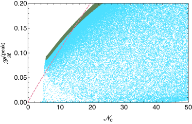
Figure 1: The peak amplitude of curvature perturbations $\mathcal{P}_{\mathcal{R}}^{(\rm peak)}$ as a function of e-folding number at the waterfall phase transition $\mathcal{N}_{\mathrm{c}}$. The dashed line represents the analytic result of Eq. (35) for the minimal model without quadratic and cubic terms. The green (blue) points represent the results with $\mu_{3}/M_{\mathrm{Pl}}\geq 1$ ($\mu_{3}/M_{\mathrm{Pl}}<1$).

The parameters that satisfy $n_{\mathrm{s}}=0.9649\pm 0.0042$ and $\mathcal{P}_{\mathcal{R}}^{(\rm peak)}\in(0.0045,0.11)$ are shown in Fig. 2 as light points. We plot the points for $\mathcal{P}_{\mathcal{R}}^{(\rm peak)}\in(0.9\mathcal{P}_{0},1.1\mathcal{P}_{0})$ with $\mathcal{P}_{0}=0.005$, $0.01$, $0.02$, $0.05$, and $0.1$ denser for a larger $\mathcal{P}_{0}$. The solid curves represent the fitting functions for $\mathcal{P}_{\mathcal{R}}^{(\rm peak)}\simeq\mathcal{P}_{0}$ with $\mathcal{P}_{0}=0.005$, $0.01$, $0.02$, $0.05$, and $0.1$ from the light to dense ones. The fitting functions are given by

$$\mathcal{N}_{\mathrm{c}}\simeq c_{\Pi,0}+c_{\Pi,1}\Pi\qquad\text{for}\quad\mathcal{N}_{\mathrm{c}}>15\,,$$ (58)

$$\mathcal{N}_{\mathrm{c}}\simeq c_{\mu_{2},0}+c_{\mu_{2},1/2}\left(\frac{\mu_{2}}{M_{\mathrm{Pl}}}\right)^{1/2}+c_{\mu_{2},1}\left(\frac{\mu_{2}}{M_{\mathrm{Pl}}}\right)\qquad\text{for}\quad\mathcal{N}_{\mathrm{c}}>15\,,$$ (59)

$$\mathcal{N}_{\mathrm{c}}\simeq c_{\mu_{3},0}+c_{\mu_{3},-3}\left(\frac{\mu_{3}}{M_{\mathrm{Pl}}}\right)^{-3}\qquad\text{for}\quad\mathcal{N}_{\mathrm{c}}>10\,,$$ (60)

for each panel in the figure. The coefficients are chosen for each $\mathcal{P}_{0}$ and are given in Table 1. The form of these functions is determined by the analytic arguments. For example, $\mathcal{N}_{\mathrm{c}}$ is proportional to $\Pi$ as indicated by Eq. (51). It is also almost independent of $\mu_{3}/M_{\mathrm{Pl}}$. This is expected from Eq. (55) with $\mu_{1}\propto\Pi^{2}\propto\mathcal{N}_{\mathrm{c}}^{2}$, by requiring that the parenthesis should be small to suppress the peak amplitude of curvature perturbations. The behavior of $\mu_{2}/M_{\mathrm{Pl}}$ is difficult to understand, but its order of magnitude is consistent with the condition to tune the parenthesis in Eq. (55) and obtain the desired value of spectral index in Eq. (37).

We also plot $\mu_{2}/M_{\mathrm{Pl}}$-$\mu_{3}/M_{\mathrm{Pl}}$ plane in Fig. 3 to clarify the correlation between these parameters. It shows that the quadratic or cubic terms have to be strong enough (i.e., $\mu_{2}/M_{\mathrm{Pl}}$ or $\mu_{3}/M_{\mathrm{Pl}}$ have to be small enough) to reduce the amplitude of curvature perturbations.

Table 1: Coefficients for fitting functions.

$\mathcal{P}_{0}$	$c_{\Pi,0}$	$c_{\Pi,1}$	$c_{\mu_{2},0}$	$c_{\mu_{2},1/2}$	$c_{\mu_{2},1}$	$c_{\mu_{3},0}$	$c_{\mu_{3},-3}$
0.1	4.6	1.4	-207	135	-17	8.6	0.33
0.05	3.2	1.3	-114	80	-9.2	-2.4	0.28
0.02	1.5	1.2	-95	71	-8.0	-20	0.27
0.01	-0.27	1.2	-103	78	-9.4	-31	0.27
0.005	-1.3	1.1	-113	86	-11	-29	0.22

Here we comment on the parameter space considered in the literature. There are many data with $\mathcal{N}_{\mathrm{c}}=\mathcal{O}(1)$ for $\mu_{2}/M_{\mathrm{Pl}}\gtrsim 6$ as shown at the bottom-right corner in the middle panel in Fig. 2. The corresponding points are not shown in the bottom panel because they require $\mu_{3}/M_{\mathrm{Pl}}\gtrsim 1$. In this parameter space, the analytic calculation at the leading order is a good approximation and hence they correspond to the case considered in Refs. [53, 54]. However, $\mathcal{P}_{\mathcal{R}}^{(\rm peak)}$ cannot be smaller than about $0.1$ in this parameter space. A parameter space with a larger $\mathcal{N}_{\mathrm{c}}$ gives a larger $\mathcal{P}_{\mathcal{R}}^{(\rm peak)}$ (see the green points in Fig. 1) . This demonstrates that astrophysical size PBHs cannot form (or are overproduced) from a hybrid inflation model if the quadratic and cubic terms for the inflaton potential are negligible. Including the latter two terms, we find the parameter space in which $\mathcal{N}_{\mathrm{c}}$ is $\mathcal{O}(10)$ and $\mathcal{P}_{\mathcal{R}}^{(\rm peak)}\sim 0.01$.

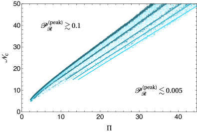
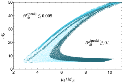
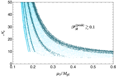
Figure 2: The e-folding number at the waterfall phase transition $\mathcal{N}_{\mathrm{c}}$ as a function of $\Pi$ (top), $\mu_{2}/M_{\mathrm{Pl}}$ (middle) $\mu_{3}/M_{\mathrm{Pl}}$, and (bottom). The solid curves represent the fitting functions for $\mathcal{P}_{\mathcal{R}}^{(\rm peak)}\simeq 0.1$, $0.05$, $0.02$, $0.01$, and $0.005$ from the dense to light ones. The lightest points include the data for $\mathcal{P}_{\mathcal{R}}^{(\rm peak)}\in(0.0045,0.11)$, whereas the dense points are the ones that are used to determine the fitting curves.

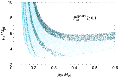
Figure 3: Same as Fig. 2 but for $\mu_{2}/M_{\mathrm{Pl}}$ as a function of $\mu_{3}/M_{\mathrm{Pl}}$.

IV PBH formation

IV.1 Press–Schechter formalism

Finally, we consider PBH formation from the collapse of overdense regions. The large curvature perturbations generated by the stochastic dynamics result in large density perturbations after inflation. If the overdensity exceeds a certain threshold, the overdense region tends to collapse to form PBHs with the size corresponding to the mode entering the horizon. The perturbation of comoving wavenumber $k$ enters the horizon when $k=a(t)H(t)$. The PBH mass is given by the total energy enclosed within the Hubble horizon at the horizon crossing:

$$M_{\rm BH} =\left.\gamma\rho\frac{4\pi H^{-3}}{3}\right|_{k=aH},$$

$$\simeq 10^{20}\ {\rm g}\left(\frac{\gamma}{0.2}\right)\left(\frac{g_{*}}{106.75}\right)^{-1/6}\left(\frac{k}{7\times 10^{12}\ {\rm Mpc}^{-1}}\right)^{-2}\,,$$ (61)

where $\gamma$ ($={\cal O}(1)$) is a numerical constant [14]. The corresponding e-folding number at the horizon exit, which we identify $\mathcal{N}_{\mathrm{c}}$, is given by

$$\mathcal{N}_{*}-\mathcal{N}_{\mathrm{c}} \simeq 32.6-\frac{1}{2}\ln\left(\frac{M_{\rm BH}}{10^{20}\,{\rm g}}\right)\,,$$ (62)

where $\mathcal{N}_{*}$ is given by Eq. (8) and we use $\gamma=0.2$ and $g_{*}=106.75$.

We can estimate the PBH abundance by the Press–Schechter theory, assuming that the density perturbations are Gaussian and that a PBH forms from a density perturbation above a certain threshold $\delta_{\mathrm{c}}$ ($\sim 0.3$). From these criteria, the probability for the PBH formation is calculated from

$$\beta(M) \equiv\frac{\rho_{\rm PBH}(M)}{\rho_{\rm tot}}\approx\int_{\delta_{\mathrm{c}}}^{\infty}\frac{\differential{\delta}}{\sqrt{2\pi\sigma^{2}(M)}}\,e^{-\frac{\delta^{2}}{2\sigma^{2}(M)}},$$

$$\simeq\sqrt{\frac{2}{\pi}}\frac{\sigma(M)}{\delta_{\mathrm{c}}}\,e^{-\frac{\delta_{\mathrm{c}}^{2}}{2\sigma^{2}(M)}}\,,$$ (63)

where $\sigma(M)$ is the variance of the coarse-grained density contrast for the scale of wavenumber $k$ corresponding to the PBH mass $M(k)$ [87]:

$$\sigma^{2}(M(1/R))=\frac{16}{81}\int\differential\ln k^{\prime}\left(k^{\prime}R\right)^{4}{\cal P}_{\mathcal{R}}(k^{\prime})\,W(k^{\prime}R)^{2},\,.$$ (64)

The window function is taken to be $W(x)=\exp\left(-x^{2}/2\right)$. The resulting PBH abundance is given by

$$f_{\rm PBH}\equiv\frac{\Omega_{\rm PBH}}{\Omega_{\rm DM}^{(\rm obs)}}\simeq\left(\frac{\beta(M)}{8\times 10^{-15}}\right)\left(\frac{M}{10^{20}\ {\rm g}}\right)^{-\frac{1}{2}}\,,\,\,\,$$ (65)

where $\Omega_{\rm DM}^{(\rm obs)}$ represents the observed DM abundance and we use $\gamma=0.2$ and $g_{*}=106.75$.

There are several constraints on the PBH abundance for a broad range of the mass scale. The shaded regions in the middle panel in Fig. 4 are excluded by evaporation (red), lensing (blue), gravitational waves (gray, GW) [88], CMB distortions (orange, PA) [89], and accretion from X-ray binaries (green, XB) [90]. For more details, the evaporation limits come from the extragalactic $\gamma$-ray background (EGB) [91, 92], the Voyager positron flux (V) [93] and annihilation-line radiation from the Galactic centre (GC) [94, 95]. The lensing constraints come from microlensing of supernovae (SN) [96] and of stars in M31 by Subaru (HSC) [97], the Magellanic Clouds by the Experience pour la Recherche d’Objets Sombres (EROS) and Massive Compact Halo Object (MACHO) collaborations (EM) [98], and the Galactic bulge by the Optical Gravitational Lensing Experiment (OGLE) (O) [99] (see also Ref. [100]). Here we assume a delta-function spectrum to illustrate the constraints [29], which should not be compared directly with our nearly-Gaussian spectrum but is useful for illustrative purpose. There is a window where PBHs can be all DM, where $M\sim 10^{17\text{--}23}\ {\rm g}$ and $\Omega_{\rm PBH}h^{2}\simeq 0.12$. Note that this requires $\mathcal{P}_{\mathcal{R}}\sim 0.01$ from Eqs. (63) and (65). The corresponding e-folding number $\mathcal{N}_{\mathrm{c}}$ should satisfy Eq. (62).

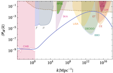
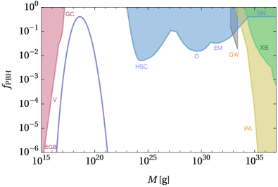
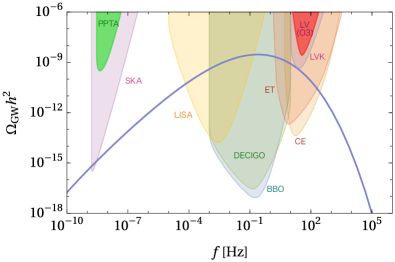
Figure 4: Spectrum of curvature perturbations $\mathcal{P}_{\mathcal{R}}$ (upper panel), PBH mass function (middle panel), and gravitational waves $\Omega_{\rm GW}h^{2}(f)$ (bottom panel) for the case with $\Pi^{2}=185$, $\mu_{2}=4.21M_{\mathrm{Pl}}$, and $\mu_{3}=0.182M_{\mathrm{Pl}}$. The shaded regions represent the constraints and future sensitivity curves (see the main text for detail).

IV.2 PBH formation in hybrid inflation model

Now we shall consider the PBH formation in the hybrid inflation model. Let us first look at the analytic result of Eqs. (51) and (55) for $\mathcal{P}_{\mathcal{R}}$ and $\mathcal{N}_{\mathrm{c}}$. If we omit the corrections from the quadratic and cubic potentials for the inflaton, which corresponds to the second and third terms in the parenthesis in Eq. (55), the peak amplitude is as large as $0.2$–$0.3$ for $\mathcal{N}_{\rm PT}\simeq 21$. This results in an overproduction of PBHs by many orders of magnitude. However, the peak amplitude can be smaller thanks to the corrections from the quadratic and cubic terms. This is the main idea of the present paper and the corresponding parameter space is demonstrated as the light blue curves in Fig. 2.

The upper panel in Fig. 4 shows the spectrum of curvature perturbations Eq. (36) with ${\cal P}_{\mathcal{R}}^{(\rm peak)}$ obtained by numerical calculation and $\chi_{k}$ given by the analytic one Eq. (52) for the case with $\Pi^{2}=185$, $\mu_{2}=4.21M_{\mathrm{Pl}}$, and $\mu_{3}=0.182M_{\mathrm{Pl}}$, which results in $\mathcal{N}_{\mathrm{c}}\simeq 17.3$, $\mathcal{P}_{\mathcal{R}}^{(\rm peak)}\simeq 0.0141$, and $n_{s}\simeq 0.969$. The corresponding PBH mass function is shown as the solid curve in the middle panel, where the peak PBH mass is $5.3\times 10^{18}\,{\rm g}$ and the total PBH abundance is $\Omega_{\rm PBH}h^{2}\simeq 0.1$. The shaded regions in the upper panel represent the excluded regions or future sensitivity curves. A parameter space with a relatively small wavenumber is excluded by constraints of CMB temperature anisotropies [101, 102, 103, 104] and $\mu$- and $y$-distortions [105, 106]. The upper-most region, denoted by the dotted curve, is excluded by the overproduction of PBHs (that partially corresponds to the shaded regions in the middle panel in Fig. 4), where we adopt the constraint for Gaussian spectrum by referring to Fig. 19 in Ref. [108].

Large curvature perturbations can generate the stochastic GW background through the second-order effect [109, 110]. We calculate the GW spectrum in hybrid inflation model and compare the result with constraints and future sensitivity curves for the GW experiments. The bottom panel in Fig. 4 shows the prediction of GW spectrum for the above-mentioned parameter. It is compared with the power-law-integrated sensitivity curves for ongoing and planned GW experiments [111]. Pulsar-timing array (PTA) experiments, such as Parkes Pulsar Timing Array (PPTA) [112] exclude the dense green shaded region. The aLIGO/aVirgo’s third observing run (LV(O3)) [113] excludes the dense red shaded region. We also plot future sensitivity curves for PTA and GW detection experiments by light shaded regions, including SKA [116], LISA [117], DECIGO [118, 119], BBO [120], Einstein Telescope (ET) [121, 122], Cosmic Explorer (CE) [123], and aLIGO+aVirgo+KAGRA (LVK) [124, 125]. The upper panel in Fig. 4 also shows them in terms of the curvature perturbations.

The case with the solid curve can be tested by future GW experiments, such as LISA. This is an interesting smoking gun signal for PBH formation in the hybrid inflation model. In particular, our GW spectrum has a relatively broad peak, which comes from the spectrum of the density curvature perturbations Eq. (36). If we can determine the GW spectrum by those experiments, we can obtain information of parameters for the hybrid inflation model, such as $\Pi$, $\mu_{2}$, and $\mu_{3}$. Then one can check the consistency with the parameter space shown in Fig. 2. One can therefore falsify or confirm our model by observations of the GW spectrum, which is actually within the future sensitivity curve.

V Discussion and conclusions

We have revisited the spectrum of curvature perturbations generated during the waterfall phase transition in a hybrid inflation model. After emphasizing the fact that the peak amplitude and wavenumber are correlated with each other in a minimal setup, we have pointed out that their degeneracy can be relaxed by quadratic and cubic terms for the inflaton potential that are omitted in the literature. In particular, PBHs with masses of the order of $10^{17\text{--}23}\,$\mathrm{g}$$ can be generated consistently with any existence constraints. Moreover, the scenario can be tested by observing GW signals induced by second-order scalar perturbations.

The peak amplitude of curvature perturbations can be reduced by the effect of quadratic and cubic terms in the inflaton potential. This requires tuning in a parameter, which we quantify as Eq. (56). The amount of tuning is, however, not that large because we need to reduce the peak amplitude only by a factor of about 10 in order not to overproduce PBHs.

Still, one has to take particular care of the tail of the spectrum for curvature perturbations. As one can see in Fig. 4 or the analytic formula Eq. (36) with Eq. (52), the spectrum generated during the waterfall phase transition is not sharp but is widely distributed over many orders of magnitude in the wavenumber. In particular, it should not affect the spectrum around the CMB scale. This constrains $\mathcal{N}_{\mathrm{c}}\lesssim 17$ for the parameters we chose throughout this paper. One can therefore generate a PBH with mass of the order of $10^{17\text{--}19}\,$\mathrm{g}$$ but cannot generate arbitrarily larger PBHs. However, this condition can be relaxed if one considers a relatively low inflation energy scale and/or low reheating temperature scenario.

Other than quadratic or cubic terms in the inflaton potential, a multiple number of waterfall fields [126, 127], a small explicit breaking of symmetry in the waterfall potential [128], etc. can be a resolution of the $\mathcal{P}_{\mathcal{R}}$-$\mathcal{N}_{\mathrm{c}}$ degeneracy. Those scenarios are motivated by avoiding the domain-wall problem in the simplest $Z_{2}$ symmetric model, where the domain walls are produced after the waterfall phase transition and then make the Universe highly inhomogeneous by dominating the energy density. In the present paper, we implicitly assumed either of these extensions to avoid the problem while their effect is negligible on the curvature perturbations. The non-Gaussian effect on PBH abundance (see, e.g., Refs. [129, 130, 5, 131, 132, 133, 134, 135, 136, 137, 138, 139, 140, 79, 72, 141, 74, 142]), its clustering (see, e.g., Refs. [143, 87, 144, 145, 146, 147, 148]), and the induced GWs (see, e.g., Refs. [149, 150, 151, 152, 153, 154, 155] and Ref. [156] for a recent review) is also an interesting topic as the perturbation generated through the waterfall transition is expected to show non-vanishing non-Gaussianity [54]. Recently, the quantum loop correction from the PBH-scale perturbation to the CMB-scale one is attracting much attention [157, 158, 159, 160, 161, 162, 163, 164, 165, 166]. Though our model is not a single-field model which conflicts with the hypothetical No-Go theorem by Ref. [158], the loop correction in this model would be worth considering. We leave them for future works.

- [1] Planck collaboration, N. Aghanim et al., Planck 2018 results. VI. Cosmological parameters, Astron. Astrophys. 641 (2020) A6 [1807.06209].
- [2] P. Ivanov, P. Naselsky and I. Novikov, Inflation and primordial black holes as dark matter, Phys. Rev. D 50 (1994) 7173.
- [3] J. Garcia-Bellido, A. D. Linde and D. Wands, Density perturbations and black hole formation in hybrid inflation, Phys. Rev. D 54 (1996) 6040 [astro-ph/9605094].
- [4] M. Kawasaki, N. Sugiyama and T. Yanagida, Primordial black hole formation in a double inflation model in supergravity, Phys. Rev. D 57 (1998) 6050 [hep-ph/9710259].
- [5] J. Yokoyama, Chaotic new inflation and formation of primordial black holes, Phys. Rev. D 58 (1998) 083510 [astro-ph/9802357].
- [6] J. Garcia-Bellido and E. Ruiz Morales, Primordial black holes from single field models of inflation, Phys. Dark Univ. 18 (2017) 47 [1702.03901].
- [7] M. P. Hertzberg and M. Yamada, Primordial Black Holes from Polynomial Potentials in Single Field Inflation, Phys. Rev. D 97 (2018) 083509 [1712.09750].
- [8] D. Lynden-Bell, Galactic nuclei as collapsed old quasars, Nature 223 (1969) 690.
- [9] J. Kormendy and D. Richstone, Inward bound: The Search for supermassive black holes in galactic nuclei, Ann. Rev. Astron. Astrophys. 33 (1995) 581.
- [10] LIGO Scientific, Virgo collaboration, B. P. Abbott et al., Binary Black Hole Mergers in the first Advanced LIGO Observing Run, Phys. Rev. X 6 (2016) 041015 [1606.04856].
- [11] LIGO Scientific, VIRGO, KAGRA collaboration, R. Abbott et al., GWTC-3: Compact Binary Coalescences Observed by LIGO and Virgo During the Second Part of the Third Observing Run, 2111.03606.
- [12] S. Hawking, Gravitationally collapsed objects of very low mass, Mon. Not. Roy. Astron. Soc. 152 (1971) 75.
- [13] B. J. Carr and S. W. Hawking, Black holes in the early Universe, Mon. Not. Roy. Astron. Soc. 168 (1974) 399.
- [14] B. J. Carr, The Primordial black hole mass spectrum, Astrophys. J. 201 (1975) 1.
- [15] S. W. Hawking, Black Holes From Cosmic Strings, Phys. Lett. B 231 (1989) 237.
- [16] J. Garriga and A. Vilenkin, Black holes from nucleating strings, Phys. Rev. D 47 (1993) 3265 [hep-ph/9208212].
- [17] R. R. Caldwell and P. Casper, Formation of black holes from collapsed cosmic string loops, Phys. Rev. D 53 (1996) 3002 [gr-qc/9509012].
- [18] S. W. Hawking, I. G. Moss and J. M. Stewart, Bubble Collisions in the Very Early Universe, Phys. Rev. D 26 (1982) 2681.
- [19] M. Y. Khlopov, Primordial Black Holes, Res. Astron. Astrophys. 10 (2010) 495 [0801.0116].
- [20] J. Garriga, A. Vilenkin and J. Zhang, Black holes and the multiverse, JCAP 02 (2016) 064 [1512.01819].
- [21] H. Deng, J. Garriga and A. Vilenkin, Primordial black hole and wormhole formation by domain walls, JCAP 04 (2017) 050 [1612.03753].
- [22] H. Deng and A. Vilenkin, Primordial black hole formation by vacuum bubbles, JCAP 12 (2017) 044 [1710.02865].
- [23] H. Deng, A. Vilenkin and M. Yamada, CMB spectral distortions from black holes formed by vacuum bubbles, JCAP 07 (2018) 059 [1804.10059].
- [24] H. Deng, Primordial black hole formation by vacuum bubbles. Part II, JCAP 09 (2020) 023 [2006.11907].
- [25] G. F. Chapline, Cosmological effects of primordial black holes, Nature 253 (1975) 251.
- [26] B. Carr, F. Kuhnel and M. Sandstad, Primordial Black Holes as Dark Matter, Phys. Rev. D 94 (2016) 083504 [1607.06077].
- [27] K. Inomata, M. Kawasaki, K. Mukaida, Y. Tada and T. T. Yanagida, Inflationary Primordial Black Holes as All Dark Matter, Phys. Rev. D 96 (2017) 043504 [1701.02544].
- [28] K. Inomata, M. Kawasaki, K. Mukaida and T. T. Yanagida, Double inflation as a single origin of primordial black holes for all dark matter and LIGO observations, Phys. Rev. D 97 (2018) 043514 [1711.06129].
- [29] A. Escrivà, F. Kuhnel and Y. Tada, Primordial Black Holes, 2211.05767.
- [30] A. D. Linde, Hybrid inflation, Phys. Rev. D 49 (1994) 748 [astro-ph/9307002].
- [31] M. Kawasaki, T. Takayama, M. Yamaguchi and J. Yokoyama, Power Spectrum of the Density Perturbations From Smooth Hybrid New Inflation Model, Phys. Rev. D 74 (2006) 043525 [hep-ph/0605271].
- [32] T. Kawaguchi, M. Kawasaki, T. Takayama, M. Yamaguchi and J. Yokoyama, Formation of intermediate-mass black holes as primordial black holes in the inflationary cosmology with running spectral index, Mon. Not. Roy. Astron. Soc. 388 (2008) 1426 [0711.3886].
- [33] K. Kohri, D. H. Lyth and A. Melchiorri, Black hole formation and slow-roll inflation, JCAP 04 (2008) 038 [0711.5006].
- [34] P. H. Frampton, M. Kawasaki, F. Takahashi and T. T. Yanagida, Primordial Black Holes as All Dark Matter, JCAP 04 (2010) 023 [1001.2308].
- [35] M. Drees and E. Erfani, Running Spectral Index and Formation of Primordial Black Hole in Single Field Inflation Models, JCAP 01 (2012) 035 [1110.6052].
- [36] M. Kawasaki, A. Kusenko and T. T. Yanagida, Primordial seeds of supermassive black holes, Phys. Lett. B 711 (2012) 1 [1202.3848].
- [37] M. Kawasaki, N. Kitajima and T. T. Yanagida, Primordial black hole formation from an axionlike curvaton model, Phys. Rev. D 87 (2013) 063519 [1207.2550].
- [38] M. Kawasaki, A. Kusenko, Y. Tada and T. T. Yanagida, Primordial black holes as dark matter in supergravity inflation models, Phys. Rev. D 94 (2016) 083523 [1606.07631].
- [39] K. Inomata, M. Kawasaki, K. Mukaida, Y. Tada and T. T. Yanagida, Inflationary primordial black holes for the LIGO gravitational wave events and pulsar timing array experiments, Phys. Rev. D 95 (2017) 123510 [1611.06130].
- [40] J. M. Ezquiaga, J. Garcia-Bellido and E. Ruiz Morales, Primordial Black Hole production in Critical Higgs Inflation, Phys. Lett. B 776 (2018) 345 [1705.04861].
- [41] K. Kannike, L. Marzola, M. Raidal and H. Veermäe, Single Field Double Inflation and Primordial Black Holes, JCAP 09 (2017) 020 [1705.06225].
- [42] C. Germani and T. Prokopec, On primordial black holes from an inflection point, Phys. Dark Univ. 18 (2017) 6 [1706.04226].
- [43] H. Motohashi and W. Hu, Primordial Black Holes and Slow-Roll Violation, Phys. Rev. D 96 (2017) 063503 [1706.06784].
- [44] G. Ballesteros and M. Taoso, Primordial black hole dark matter from single field inflation, Phys. Rev. D 97 (2018) 023501 [1709.05565].
- [45] M. Cicoli, V. A. Diaz and F. G. Pedro, Primordial Black Holes from String Inflation, JCAP 06 (2018) 034 [1803.02837].
- [46] D. Y. Cheong, S. M. Lee and S. C. Park, Primordial black holes in Higgs- inflation as the whole of dark matter, JCAP 01 (2021) 032 [1912.12032].
- [47] G. Ballesteros, J. Rey, M. Taoso and A. Urbano, Primordial black holes as dark matter and gravitational waves from single-field polynomial inflation, JCAP 07 (2020) 025 [2001.08220].
- [48] S. Pi and M. Sasaki, Primordial Black Hole Formation in Non-Minimal Curvaton Scenario, 2112.12680.
- [49] S. R. Geller, W. Qin, E. McDonough and D. I. Kaiser, Primordial black holes from multifield inflation with nonminimal couplings, Phys. Rev. D 106 (2022) 063535 [2205.04471].
- [50] S. Clesse, Hybrid inflation along waterfall trajectories, Phys. Rev. D 83 (2011) 063518 [1006.4522].
- [51] H. Kodama, K. Kohri and K. Nakayama, On the waterfall behavior in hybrid inflation, Prog. Theor. Phys. 126 (2011) 331 [1102.5612].
- [52] D. Mulryne, S. Orani and A. Rajantie, Non-Gaussianity from the hybrid potential, Phys. Rev. D 84 (2011) 123527 [1107.4739].
- [53] S. Clesse and J. García-Bellido, Massive Primordial Black Holes from Hybrid Inflation as Dark Matter and the seeds of Galaxies, Phys. Rev. D 92 (2015) 023524 [1501.07565].
- [54] M. Kawasaki and Y. Tada, Can massive primordial black holes be produced in mild waterfall hybrid inflation?, JCAP 08 (2016) 041 [1512.03515].
- [55] A. A. Starobinsky, Dynamics of Phase Transition in the New Inflationary Universe Scenario and Generation of Perturbations, Phys. Lett. B 117 (1982) 175.
- [56] A. A. Starobinsky, STOCHASTIC DE SITTER (INFLATIONARY) STAGE IN THE EARLY UNIVERSE, Lect. Notes Phys. 246 (1986) 107.
- [57] Y. Nambu and M. Sasaki, Stochastic Stage of an Inflationary Universe Model, Phys. Lett. B 205 (1988) 441.
- [58] Y. Nambu and M. Sasaki, Stochastic Approach to Chaotic Inflation and the Distribution of Universes, Phys. Lett. B 219 (1989) 240.
- [59] H. E. Kandrup, STOCHASTIC INFLATION AS A TIME DEPENDENT RANDOM WALK, Phys. Rev. D 39 (1989) 2245.
- [60] K.-i. Nakao, Y. Nambu and M. Sasaki, Stochastic Dynamics of New Inflation, Prog. Theor. Phys. 80 (1988) 1041.
- [61] Y. Nambu, Stochastic Dynamics of an Inflationary Model and Initial Distribution of Universes, Prog. Theor. Phys. 81 (1989) 1037.
- [62] S. Mollerach, S. Matarrese, A. Ortolan and F. Lucchin, Stochastic inflation in a simple two field model, Phys. Rev. D 44 (1991) 1670.
- [63] A. D. Linde, D. A. Linde and A. Mezhlumian, From the Big Bang theory to the theory of a stationary universe, Phys. Rev. D 49 (1994) 1783 [gr-qc/9306035].
- [64] A. A. Starobinsky and J. Yokoyama, Equilibrium state of a selfinteracting scalar field in the De Sitter background, Phys. Rev. D 50 (1994) 6357 [astro-ph/9407016].
- [65] V. C. Spanos and I. D. Stamou, Gravitational waves and primordial black holes from supersymmetric hybrid inflation, Phys. Rev. D 104 (2021) 123537 [2108.05671].
- [66] A. A. Starobinsky, Multicomponent de Sitter (Inflationary) Stages and the Generation of Perturbations, JETP Lett. 42 (1985) 152.
- [67] D. S. Salopek and J. R. Bond, Nonlinear evolution of long wavelength metric fluctuations in inflationary models, Phys. Rev. D 42 (1990) 3936.
- [68] M. Sasaki and E. D. Stewart, A General analytic formula for the spectral index of the density perturbations produced during inflation, Prog. Theor. Phys. 95 (1996) 71 [astro-ph/9507001].
- [69] M. Sasaki and T. Tanaka, Superhorizon scale dynamics of multiscalar inflation, Prog. Theor. Phys. 99 (1998) 763 [gr-qc/9801017].
- [70] D. H. Lyth, K. A. Malik and M. Sasaki, A General proof of the conservation of the curvature perturbation, JCAP 05 (2005) 004 [astro-ph/0411220].
- [71] C.-M. Yoo, T. Harada, J. Garriga and K. Kohri, Primordial black hole abundance from random Gaussian curvature perturbations and a local density threshold, PTEP 2018 (2018) 123E01 [1805.03946].
- [72] C.-M. Yoo, J.-O. Gong and S. Yokoyama, Abundance of primordial black holes with local non-Gaussianity in peak theory, JCAP 09 (2019) 033 [1906.06790].
- [73] C.-M. Yoo, T. Harada, S. Hirano and K. Kohri, Abundance of Primordial Black Holes in Peak Theory for an Arbitrary Power Spectrum, PTEP 2021 (2021) 013E02 [2008.02425].
- [74] N. Kitajima, Y. Tada, S. Yokoyama and C.-M. Yoo, Primordial black holes in peak theory with a non-Gaussian tail, JCAP 10 (2021) 053 [2109.00791].
- [75] M. Shibata and M. Sasaki, Black hole formation in the Friedmann universe: Formulation and computation in numerical relativity, Phys. Rev. D 60 (1999) 084002 [gr-qc/9905064].
- [76] T. Harada, C.-M. Yoo, T. Nakama and Y. Koga, Cosmological long-wavelength solutions and primordial black hole formation, Phys. Rev. D 91 (2015) 084057 [1503.03934].
- [77] S. Young, I. Musco and C. T. Byrnes, Primordial black hole formation and abundance: contribution from the non-linear relation between the density and curvature perturbation, JCAP 11 (2019) 012 [1904.00984].
- [78] A. Escrivà, C. Germani and R. K. Sheth, Universal threshold for primordial black hole formation, Phys. Rev. D 101 (2020) 044022 [1907.13311].
- [79] V. Atal, J. Cid, A. Escrivà and J. Garriga, PBH in single field inflation: the effect of shape dispersion and non-Gaussianities, JCAP 05 (2020) 022 [1908.11357].
- [80] M. W. Choptuik, Universality and scaling in gravitational collapse of a massless scalar field, Phys. Rev. Lett. 70 (1993) 9.
- [81] C. R. Evans and J. S. Coleman, Observation of critical phenomena and selfsimilarity in the gravitational collapse of radiation fluid, Phys. Rev. Lett. 72 (1994) 1782 [gr-qc/9402041].
- [82] T. Koike, T. Hara and S. Adachi, Critical behavior in gravitational collapse of radiation fluid: A Renormalization group (linear perturbation) analysis, Phys. Rev. Lett. 74 (1995) 5170 [gr-qc/9503007].
- [83] J. C. Niemeyer and K. Jedamzik, Near-critical gravitational collapse and the initial mass function of primordial black holes, Phys. Rev. Lett. 80 (1998) 5481 [astro-ph/9709072].
- [84] J. C. Niemeyer and K. Jedamzik, Dynamics of primordial black hole formation, Phys. Rev. D 59 (1999) 124013 [astro-ph/9901292].
- [85] I. Hawke and J. M. Stewart, The dynamics of primordial black hole formation, Class. Quant. Grav. 19 (2002) 3687.
- [86] I. Musco, J. C. Miller and A. G. Polnarev, Primordial black hole formation in the radiative era: Investigation of the critical nature of the collapse, Class. Quant. Grav. 26 (2009) 235001 [0811.1452].
- [87] S. Young, C. T. Byrnes and M. Sasaki, Calculating the mass fraction of primordial black holes, JCAP 07 (2014) 045 [1405.7023].
- [88] M. Raidal, V. Vaskonen and H. Veermäe, Gravitational Waves from Primordial Black Hole Mergers, JCAP 09 (2017) 037 [1707.01480].
- [89] P. D. Serpico, V. Poulin, D. Inman and K. Kohri, Cosmic microwave background bounds on primordial black holes including dark matter halo accretion, Phys. Rev. Res. 2 (2020) 023204 [2002.10771].
- [90] Y. Inoue and A. Kusenko, New X-ray bound on density of primordial black holes, JCAP 10 (2017) 034 [1705.00791].
- [91] D. N. Page and S. W. Hawking, Gamma rays from primordial black holes, Astrophys. J. 206 (1976) 1.
- [92] B. J. Carr, K. Kohri, Y. Sendouda and J. Yokoyama, New cosmological constraints on primordial black holes, Phys. Rev. D 81 (2010) 104019 [0912.5297].
- [93] M. Boudaud and M. Cirelli, Voyager 1 Further Constrain Primordial Black Holes as Dark Matter, Phys. Rev. Lett. 122 (2019) 041104 [1807.03075].
- [94] R. Laha, Primordial Black Holes as a Dark Matter Candidate Are Severely Constrained by the Galactic Center 511 keV -Ray Line, Phys. Rev. Lett. 123 (2019) 251101 [1906.09994].
- [95] W. DeRocco and P. W. Graham, Constraining Primordial Black Hole Abundance with the Galactic 511 keV Line, Phys. Rev. Lett. 123 (2019) 251102 [1906.07740].
- [96] M. Zumalacarregui and U. Seljak, Limits on stellar-mass compact objects as dark matter from gravitational lensing of type Ia supernovae, Phys. Rev. Lett. 121 (2018) 141101 [1712.02240].
- [97] H. Niikura et al., Microlensing constraints on primordial black holes with Subaru/HSC Andromeda observations, Nature Astron. 3 (2019) 524 [1701.02151].
- [98] T. Blaineau et al., New limits from microlensing on Galactic black holes in the mass range 10 M M 1000 M, Astron. Astrophys. 664 (2022) A106 [2202.13819].
- [99] L. Wyrzykowski et al., The OGLE View of Microlensing towards the Magellanic Clouds. IV. OGLE-III SMC Data and Final Conclusions on MACHOs, Mon. Not. Roy. Astron. Soc. 416 (2011) 2949 [1106.2925].
- [100] H. Niikura, M. Takada, S. Yokoyama, T. Sumi and S. Masaki, Constraints on Earth-mass primordial black holes from OGLE 5-year microlensing events, Phys. Rev. D 99 (2019) 083503 [1901.07120].
- [101] G. Nicholson and C. R. Contaldi, Reconstruction of the Primordial Power Spectrum using Temperature and Polarisation Data from Multiple Experiments, JCAP 07 (2009) 011 [0903.1106].
- [102] G. Nicholson, C. R. Contaldi and P. Paykari, Reconstruction of the Primordial Power Spectrum by Direct Inversion, JCAP 01 (2010) 016 [0909.5092].
- [103] S. Bird, H. V. Peiris, M. Viel and L. Verde, Minimally Parametric Power Spectrum Reconstruction from the Lyman-alpha Forest, Mon. Not. Roy. Astron. Soc. 413 (2011) 1717 [1010.1519].
- [104] T. Bringmann, P. Scott and Y. Akrami, Improved constraints on the primordial power spectrum at small scales from ultracompact minihalos, Phys. Rev. D 85 (2012) 125027 [1110.2484].
- [105] D. J. Fixsen, E. S. Cheng, J. M. Gales, J. C. Mather, R. A. Shafer and E. L. Wright, The Cosmic Microwave Background spectrum from the full COBE FIRAS data set, Astrophys. J. 473 (1996) 576 [astro-ph/9605054].
- [106] J. Chluba, A. L. Erickcek and I. Ben-Dayan, Probing the inflaton: Small-scale power spectrum constraints from measurements of the CMB energy spectrum, Astrophys. J. 758 (2012) 76 [1203.2681].
- [107] F. Bianchini and G. Fabbian, CMB spectral distortions revisited: A new take on distortions and primordial non-Gaussianities from FIRAS data, Phys. Rev. D 106 (2022) 063527 [2206.02762].
- [108] B. Carr, K. Kohri, Y. Sendouda and J. Yokoyama, Constraints on primordial black holes, Rept. Prog. Phys. 84 (2021) 116902 [2002.12778].
- [109] R. Saito and J. Yokoyama, Gravitational wave background as a probe of the primordial black hole abundance, Phys. Rev. Lett. 102 (2009) 161101 [0812.4339].
- [110] R. Saito and J. Yokoyama, Gravitational-Wave Constraints on the Abundance of Primordial Black Holes, Prog. Theor. Phys. 123 (2010) 867 [0912.5317].
- [111] K. Schmitz, New Sensitivity Curves for Gravitational-Wave Signals from Cosmological Phase Transitions, JHEP 01 (2021) 097 [2002.04615].
- [112] R. M. Shannon et al., Gravitational waves from binary supermassive black holes missing in pulsar observations, Science 349 (2015) 1522 [1509.07320].
- [113] KAGRA, Virgo, LIGO Scientific collaboration, R. Abbott et al., Upper limits on the isotropic gravitational-wave background from Advanced LIGO and Advanced Virgo’s third observing run, Phys. Rev. D 104 (2021) 022004 [2101.12130].
- [114] S. J. Kapadia, K. Lal Pandey, T. Suyama, S. Kandhasamy and P. Ajith, Search for the Stochastic Gravitational-wave Background Induced by Primordial Curvature Perturbations in LIGO’s Second Observing Run, Astrophys. J. Lett. 910 (2021) L4 [2009.05514].
- [115] A. Romero-Rodriguez, M. Martinez, O. Pujolàs, M. Sakellariadou and V. Vaskonen, Search for a Scalar Induced Stochastic Gravitational Wave Background in the Third LIGO-Virgo Observing Run, Phys. Rev. Lett. 128 (2022) 051301 [2107.11660].
- [116] G. Janssen et al., Gravitational wave astronomy with the SKA, PoS AASKA14 (2015) 037 [1501.00127].
- [117] LISA collaboration, P. Amaro-Seoane et al., Laser Interferometer Space Antenna, 1702.00786.
- [118] S. Kawamura et al., The Japanese space gravitational wave antenna: DECIGO, Class. Quant. Grav. 28 (2011) 094011.
- [119] S. Kawamura et al., Current status of space gravitational wave antenna DECIGO and B-DECIGO, PTEP 2021 (2021) 05A105 [2006.13545].
- [120] G. M. Harry, P. Fritschel, D. A. Shaddock, W. Folkner and E. S. Phinney, Laser interferometry for the big bang observer, Class. Quant. Grav. 23 (2006) 4887.
- [121] M. Punturo et al., The Einstein Telescope: A third-generation gravitational wave observatory, Class. Quant. Grav. 27 (2010) 194002.
- [122] M. Maggiore et al., Science Case for the Einstein Telescope, JCAP 03 (2020) 050 [1912.02622].
- [123] D. Reitze et al., Cosmic Explorer: The U.S. Contribution to Gravitational-Wave Astronomy beyond LIGO, Bull. Am. Astron. Soc. 51 (2019) 035 [1907.04833].
- [124] KAGRA collaboration, K. Somiya, Detector configuration of KAGRA: The Japanese cryogenic gravitational-wave detector, Class. Quant. Grav. 29 (2012) 124007 [1111.7185].
- [125] KAGRA collaboration, T. Akutsu et al., Overview of KAGRA : KAGRA science, 2008.02921.
- [126] I. F. Halpern, M. P. Hertzberg, M. A. Joss and E. I. Sfakianakis, A Density Spike on Astrophysical Scales from an N-Field Waterfall Transition, Phys. Lett. B 748 (2015) 132 [1410.1878].
- [127] Y. Tada and M. Yamada, Stochastic dynamics of multi-waterfall hybrid inflation and formation of primordial black holes, 2306.07324.
- [128] M. Braglia, A. Linde, R. Kallosh and F. Finelli, Hybrid -attractors, primordial black holes and gravitational wave backgrounds, 2211.14262.
- [129] J. S. Bullock and J. R. Primack, NonGaussian fluctuations and primordial black holes from inflation, Phys. Rev. D 55 (1997) 7423 [astro-ph/9611106].
- [130] P. Ivanov, Nonlinear metric perturbations and production of primordial black holes, Phys. Rev. D 57 (1998) 7145 [astro-ph/9708224].
- [131] J. C. Hidalgo, The effect of non-Gaussian curvature perturbations on the formation of primordial black holes, 0708.3875.
- [132] C. T. Byrnes, E. J. Copeland and A. M. Green, Primordial black holes as a tool for constraining non-Gaussianity, Phys. Rev. D 86 (2012) 043512 [1206.4188].
- [133] E. V. Bugaev and P. A. Klimai, Primordial black hole constraints for curvaton models with predicted large non-Gaussianity, Int. J. Mod. Phys. D 22 (2013) 1350034 [1303.3146].
- [134] S. Young, D. Regan and C. T. Byrnes, Influence of large local and non-local bispectra on primordial black hole abundance, JCAP 02 (2016) 029 [1512.07224].
- [135] T. Nakama, J. Silk and M. Kamionkowski, Stochastic gravitational waves associated with the formation of primordial black holes, Phys. Rev. D 95 (2017) 043511 [1612.06264].
- [136] K. Ando, K. Inomata, M. Kawasaki, K. Mukaida and T. T. Yanagida, Primordial black holes for the LIGO events in the axionlike curvaton model, Phys. Rev. D 97 (2018) 123512 [1711.08956].
- [137] G. Franciolini, A. Kehagias, S. Matarrese and A. Riotto, Primordial Black Holes from Inflation and non-Gaussianity, JCAP 03 (2018) 016 [1801.09415].
- [138] V. Atal and C. Germani, The role of non-gaussianities in Primordial Black Hole formation, Phys. Dark Univ. 24 (2019) 100275 [1811.07857].
- [139] S. Passaglia, W. Hu and H. Motohashi, Primordial black holes and local non-Gaussianity in canonical inflation, Phys. Rev. D 99 (2019) 043536 [1812.08243].
- [140] V. Atal, J. Garriga and A. Marcos-Caballero, Primordial black hole formation with non-Gaussian curvature perturbations, JCAP 09 (2019) 073 [1905.13202].
- [141] M. Taoso and A. Urbano, Non-gaussianities for primordial black hole formation, JCAP 08 (2021) 016 [2102.03610].
- [142] A. Escrivà, Y. Tada, S. Yokoyama and C.-M. Yoo, Simulation of primordial black holes with large negative non-Gaussianity, JCAP 05 (2022) 012 [2202.01028].
- [143] J. R. Chisholm, Clustering of primordial black holes: basic results, Phys. Rev. D 73 (2006) 083504 [astro-ph/0509141].
- [144] S. Young and C. T. Byrnes, Long-short wavelength mode coupling tightens primordial black hole constraints, Phys. Rev. D 91 (2015) 083521 [1411.4620].
- [145] Y. Tada and S. Yokoyama, Primordial black holes as biased tracers, Phys. Rev. D 91 (2015) 123534 [1502.01124].
- [146] S. Young and C. T. Byrnes, Signatures of non-gaussianity in the isocurvature modes of primordial black hole dark matter, JCAP 04 (2015) 034 [1503.01505].
- [147] T. Suyama and S. Yokoyama, Clustering of primordial black holes with non-Gaussian initial fluctuations, PTEP 2019 (2019) 103E02 [1906.04958].
- [148] S. Young and C. T. Byrnes, Initial clustering and the primordial black hole merger rate, JCAP 03 (2020) 004 [1910.06077].
- [149] R.-g. Cai, S. Pi and M. Sasaki, Gravitational Waves Induced by non-Gaussian Scalar Perturbations, Phys. Rev. Lett. 122 (2019) 201101 [1810.11000].
- [150] C. Unal, Imprints of Primordial Non-Gaussianity on Gravitational Wave Spectrum, Phys. Rev. D 99 (2019) 041301 [1811.09151].
- [151] C. Yuan and Q.-G. Huang, Gravitational waves induced by the local-type non-Gaussian curvature perturbations, Phys. Lett. B 821 (2021) 136606 [2007.10686].
- [152] V. Atal and G. Domènech, Probing non-Gaussianities with the high frequency tail of induced gravitational waves, JCAP 06 (2021) 001 [2103.01056].
- [153] P. Adshead, K. D. Lozanov and Z. J. Weiner, Non-Gaussianity and the induced gravitational wave background, JCAP 10 (2021) 080 [2105.01659].
- [154] S. Garcia-Saenz, L. Pinol, S. Renaux-Petel and D. Werth, No-go Theorem for Scalar-Trispectrum-Induced Gravitational Waves, 2207.14267.
- [155] K. T. Abe, R. Inui, Y. Tada and S. Yokoyama, Primordial black holes and gravitational waves induced by exponential-tailed perturbations, 2209.13891.
- [156] G. Domènech, Scalar Induced Gravitational Waves Review, Universe 7 (2021) 398 [2109.01398].
- [157] K. Inomata, M. Braglia and X. Chen, Questions on calculation of primordial power spectrum with large spikes: the resonance model case, JCAP 04 (2023) 011 [2211.02586].
- [158] J. Kristiano and J. Yokoyama, Ruling Out Primordial Black Hole Formation From Single-Field Inflation, 2211.03395.
- [159] A. Riotto, The Primordial Black Hole Formation from Single-Field Inflation is Not Ruled Out, 2301.00599.
- [160] S. Choudhury, M. R. Gangopadhyay and M. Sami, No-go for the formation of heavy mass Primordial Black Holes in Single Field Inflation, 2301.10000.
- [161] S. Choudhury, S. Panda and M. Sami, No-go for PBH formation in EFT of single field inflation, 2302.05655.
- [162] J. Kristiano and J. Yokoyama, Response to criticism on ”Ruling Out Primordial Black Hole Formation From Single-Field Inflation”: A note on bispectrum and one-loop correction in single-field inflation with primordial black hole formation, 2303.00341.
- [163] A. Riotto, The Primordial Black Hole Formation from Single-Field Inflation is Still Not Ruled Out, 2303.01727.
- [164] S. Choudhury, S. Panda and M. Sami, Quantum loop effects on the power spectrum and constraints on primordial black holes, 2303.06066.
- [165] H. Firouzjahi, One-loop Corrections in Power Spectrum in Single Field Inflation, 2303.12025.
- [166] H. Motohashi and Y. Tada, Squeezed bispectrum and one-loop corrections in transient constant-roll inflation, 2303.16035.