Generative Diffusion Prior for Unified Image Restoration and Enhancement

Abstract

Existing image restoration methods mostly leverage the posterior distribution of natural images. However, they often assume known degradation and also require supervised training, which restricts their adaptation to complex real applications. In this work, we propose the Generative Diffusion Prior (GDP) to effectively model the posterior distributions in an unsupervised sampling manner. GDP utilizes a pre-train denoising diffusion generative model (DDPM) for solving linear inverse, non-linear, or blind problems. Specifically, GDP systematically explores a protocol of conditional guidance, which is verified more practical than the commonly used guidance way. Furthermore, GDP is strength at optimizing the parameters of degradation model during the denoising process, achieving blind image restoration. Besides, we devise hierarchical guidance and patch-based methods, enabling the GDP to generate images of arbitrary resolutions. Experimentally, we demonstrate GDP ’s versatility on several image datasets for linear problems, such as super-resolution, deblurring, inpainting, and colorization, as well as non-linear and blind issues, such as low-light enhancement and HDR image recovery. GDP outperforms the current leading unsupervised methods on the diverse benchmarks in reconstruction quality and perceptual quality. Moreover, GDP also generalizes well for natural images or synthesized images with arbitrary sizes from various tasks out of the distribution of the ImageNet training set. The project page is available at https://generativediffusionprior.github.io/

1 Introduction

Image quality often degrades during capture, storage, transmission, and rendering. Image restoration and enhancement [44] aim to inverse the degradation and improve the image quality. Typically, restoration and enhancement tasks can be divided into two main categories: 1) Linear inverse problems, such as image super-resolution (SR) [24, 39], deblurring [37, 80], inpainting [93], colorization [38, 100], where the degradation model is usually linear and known; 2) Non-linear or blind problems [1], such as image low-light enhancement [41] and HDR image recovery [10, 84], where the degradation model is non-linear and unknown. For a specific linear degradation model, image restoration can be tackled through end-to-end supervised training of neural networks [16, 100]. Nonetheless, corrupted images in the real world often have multiple complex degradations [60], where fully supervised approaches suffer to generalize.

There is a surge of interest to seek for more general image priors through generative models [74, 21, 1], and tackle image restoration in an unsupervised setting [8, 19], where multiple restoration tasks of different degradation models can be addressed during inference without re-training. For instance, Generative Adversarial Networks (GANs) [20] that are trained on a large dataset of clean images learn rich knowledge of the real-world scenes have succeeded in various linear inverse problems through GAN inversion [62, 54, 21]. In parallel, Denoising Diffusion Probabilistic Models (DDPMs) [2, 7, 36, 82, 72, 77] have demonstrated impressive generative capabilities, level of details, and diversity on top of GAN [27, 76, 78, 81, 67, 66]. As an early attempt, Kawar et al. [32] explore pre-trained DDPMs with variational inference, and achieve satisfactory results on multiple restoration tasks, but their Denoising Diffusion Restoration Model (DDRM) leverages the singular value decomposition (SVD) on a known linear degradation matrix, making it still limited to linear inverse problems.

In this study, we take a step further and propose an efficient approach named Generative Diffusion Prior (GDP). It exploits a well-trained DDPM as effective prior for general-purpose image restoration and enhancement, using degraded image as guidance. As a unified framework, GDP not only works on various linear inverse problems, but also generalizes to non-linear, and blind image restoration and enhancement tasks for the first time. However, solving the blind inverse problem is not trivial, as one would need to concurrently estimate the degradation model and recover the clean image with high fidelity. Thanks to the generative prior in a pre-trained DDPM, denoising within the DDPM manifold naturally regularizes the realness and fidelity of the recovered image. Therefore, we adopt a blind degradation estimation strategy, where the degradation model parameters of GDP are randomly initialized and optimized during the denoising process. Moreover, to further improve the photorealism and image quality, we systematically investigate an effective way to guide the diffusion models. Specifically, in the sampling process, the pre-trained DDPM first predicts a clean image $\boldsymbol{\tilde{x}}_{0}$ from the noisy image $\boldsymbol{x}_{t}$ by estimating the noise in $\boldsymbol{x}_{t}$. We can add guidance on this intermediate variable $\boldsymbol{\tilde{x}}_{0}$ to control the generation process of the DDPMs. In addition, with the help of the proposed hierarchical guidance and patch-based generation strategy, GDP is able to recover images of arbitrary resolutions, where low-resolution images and degradation models are first predicted to guide the generation of high-resolution images.

We demonstrate the empirical effectiveness of GDP by comparing it with various competitive unsupervised methods under the linear or multi-linear inverse problem on ImageNet [14], LSUN [94], and CelebA [31] datasets in terms of consistency and FID. Over the low-light [41] and NTIRE [63] datasets, we further show GDP results on non-linear and blind issues, including low-light enhancement and HDR recovery, superior to other zero-shot baselines both qualitatively and quantitively, manifesting that GDP trained on ImageNet also works on images out of its training set distribution.

Our contributions are fourfold: (1) To our best knowledge, GDP is the first unified problem solver that can effectively use a single unconditional DDPM pre-trained on ImageNet provide by [15] to produce diverse and high-fidelity outputs for unified image restoration and enhancement in an unsupervised manner. (2) GDP is capable of optimizing randomly initiated parameters of degradation that are unknown, resulting in a powerful framework that can tackle any blind image restoration. (3) Further, to achieve arbitrary size image generation, we propose hierarchical guidance and patch-based methods, greatly promoting GDP on natural image enhancement. (4) Moreover, the comprehensive experiments are carried out, different from the conventional guidance way, where GDP directly predicts the temporary output given the noisy image in every step, which will be leveraged to guide the generation of images in the next step.

2 Related works

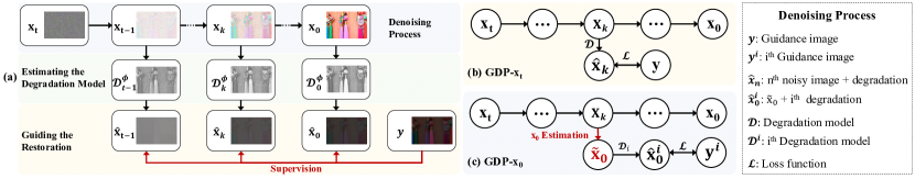
Figure 2: Overview of our GDP for unified image recovery. (a) Given a corrupted image $\boldsymbol{y}$ during inference, GDP systematically studies the reverse process from $\boldsymbol{x}_{T}$ to $\boldsymbol{x}_{0}$ guided by the $\boldsymbol{y}$. The guidance can be added on $\boldsymbol{\hat{x}}_{0}$ or $\boldsymbol{\hat{x}}_{t}$, leading to two variants of GDP. And $\boldsymbol{\hat{x}}_{0}$ and $\boldsymbol{\hat{x}}_{t}$ can be collectively expressed as $\boldsymbol{\hat{x}_{t}}$. The supervision signal (Sec. 5) is applied between $\boldsymbol{\hat{x}_{t}}$ and $\boldsymbol{y}$. GDP looks for an intermediate variable $\boldsymbol{x}_{t}$ and optimizes the degradation model $\{\mathcal{D}^{i}_{\phi}\mid i=1,2,\ldots,n\}$ that best reconstruct the image corresponding to $\boldsymbol{y}$ via gradient descent. Note that GDP is a generic image restoration method. We illustrate it with the low light enhancement example. (b) GDP-$\boldsymbol{x}_{t}$ adds guidance $\boldsymbol{x}_{t}$ in every time step (Algo.  1), while (c) GDP-$\boldsymbol{x}_{0}$ estimates the $\boldsymbol{\tilde{x}}_{0}$ given $\boldsymbol{x}_{t}$, then adds guidance on $\boldsymbol{\tilde{x}}_{0}$ to obtain $\boldsymbol{\hat{x}}_{0}$(Algo.  2). The number of guidance images $\{\boldsymbol{y}^{i}\mid i=1,2,\ldots,n\}$ and the degradation models $\{\mathcal{D}^{i}_{\phi}\mid i=1,2,\ldots,n\}$ are dependent on the tasks. For instance, $n=3$ for HDR recovery, while $n=1$ for other tasks.

Linear Inverse Image Restoration. Most diffusion models toward linear inverse problems have employed unconditional models for the conditional tasks[53, 79], where only one model needs to be trained. However, unconditional tasks tend to be more difficult than conditional tasks. Moreover, the multi-linear task is also a relatively under-explored subject in image restoration. For instance, [65, 95] train simultaneously on multiple tasks, but they mainly concentrate on the enhancement tasks like deblurring and so on. Some works have also handled the multi-scale super-resolution by simultaneous training over multiple degradations [35]. Here, we propose GDP as a single model for dealing with single linear inverse or multiple linear inverse tasks.

Non-linear Image Restoration. The non-linear image formation model provides an accurate description of several imaging systems, including camera response functions in high-dynamic-range imaging[68]. The non-linear image restoration model is more accurate but is often more computationally intractable. Recently, great attention has been paid to non-linear image restoration problems. For example, HDR-GAN [59] is proposed for synthesizing HDR images from multi-exposed LDR images, while EnlightenGAN [29] is devised as an unsupervised GAN to generalize very well on various real-world test images. The diffusion models are rarely studied for non-linear image restoration.

Blind Image Restoration. Early supervised attempts [5, 25] tend to estimate the unknown point spread function. As an example, [34] designs a class of structured denoisers, and  [75] employs a fixed down-sampling operation to generate synthetic pairs during testing. However, these methods often are incapable of obtaining the parameters or distribution of the observed data due to the complicated degradation types. Another way to solve the blind image restoration is to utilize unsupervised learning methods [107, 18]. Following the CycleGAN [107], CinCGAN [96] and MCinCGAN [103] employ a pre-trained SR model together with cycle consistency loss to learn a mapping from the input image to high-quality image space. However, it still remains a challenge to exploit a unified architecture for blind image restoration. By the merits of the powerful GDP, these blind problems could also be solved by simultaneously estimating the recovered image and a specific degradation model.

3 Preliminary

Diffusion models [71, 89, 22, 2, 36] transform complex data distribution $\boldsymbol{x}_{0}\sim p_{\text{data}}$ into simple noise distribution $\boldsymbol{x}_{T}\sim p_{\text{latent }}=\mathcal{N}\left(\mathbf{0},\boldsymbol{I}\right)$ and recover data from noise, where $\mathcal{N}$ is the Gaussian distribution. DDPMs mainly comprise the diffusion process and the reverse process.

The Diffusion Process is a Markov chain that gradually corrupts data $\boldsymbol{x}_{0}$ until it approaches Gaussian noise $p_{\text{latent }}$ at $T$ diffusion time steps. Corrupted data $\boldsymbol{x}_{1},\ldots,\boldsymbol{x}_{T}$ are sampled from data $p_{\text{data}}$, with a diffusion process, which is defined as Gaussian transition:

$$\vspace{-0.1cm}\!\!q\left(\boldsymbol{x}_{1},\cdots,\boldsymbol{x}_{T}\mid\boldsymbol{x}_{0}\right)=\prod_{t=1}^{T}q\left(\boldsymbol{x}_{t}\mid\boldsymbol{x}_{t-1}\right),\vspace{-0.1cm}$$ (1)

where $t$ denotes as diffusion step, $q\left(\boldsymbol{x}_{t}\mid\boldsymbol{x}_{t-1}\right)=\mathcal{N}\left(\boldsymbol{x}_{t};\sqrt{1-\beta_{t}}\boldsymbol{x}_{t-1},\beta_{t}\boldsymbol{I}\right)$, and $\beta_{t}$ are fixed or learned variance schedule. An important property of the forward noising process is that any step $\boldsymbol{x}_{t}$ may be sampled directly from $\boldsymbol{x}_{0}$ through the following equation:

$$\begin{split}&\boldsymbol{x}_{t}=\sqrt{\bar{\alpha}_{t}}\boldsymbol{x}_{0}+\sqrt{1-\bar{\alpha}_{t}}\boldsymbol{\epsilon},\end{split}$$ (2)

where $\boldsymbol{\epsilon}\sim\mathcal{N}(0,\boldsymbol{I})$, $\alpha_{t}=1-\beta_{t}$ and $\bar{\alpha}_{t}=\prod_{i=1}^{t}\alpha_{i}$. Proved by Ho et al. [27], there is a closed form expression for $q\left(\boldsymbol{x}_{t}\mid\boldsymbol{x}_{0}\right)$. We can obtain $q\left(\boldsymbol{x}_{t}\mid\boldsymbol{x}_{0}\right)=$ $\mathcal{N}\left(\boldsymbol{x}_{t};\sqrt{\bar{\alpha}_{t}}\boldsymbol{x}_{0},\left(1-\bar{\alpha}_{t}\right)\boldsymbol{I}\right)$. Herein, $\bar{\alpha}_{t}$ goes to 0 with large $T$, and $q\left(\boldsymbol{x}_{T}\mid\boldsymbol{x}_{0}\right)$ is close to the latent distribution $p_{\text{latent }}$.

The Reverse Process is a Markov chain that iteratively denoises a sampled Gaussian noise to a clean image. Starting from noise $x_{T}\sim\mathcal{N}(0,\boldsymbol{I})$, the reverse process from latent $\boldsymbol{x}_{T}$ to clean data $\boldsymbol{x}_{0}$ is defined as:

$$\begin{split}&p_{\boldsymbol{\theta}}\left(\boldsymbol{x}_{0},\cdots,\boldsymbol{x}_{T-1}\mid\boldsymbol{x}_{T}\right)=\prod_{t=1}^{T}p_{\boldsymbol{\theta}}\left(\boldsymbol{x}_{t-1}\mid\boldsymbol{x}_{t}\right),\quad\\ &p_{\boldsymbol{\theta}}\left(\boldsymbol{x}_{t-1}\mid\boldsymbol{x}_{t}\right)=\mathcal{N}\left(\boldsymbol{x}_{t-1};\boldsymbol{\mu}_{\boldsymbol{\theta}}\left(\boldsymbol{x}_{t},t\right),\Sigma_{\theta}\boldsymbol{I}\right)\end{split}$$ (3)

According to Ho et al. [27], the mean $\boldsymbol{\mu}_{\boldsymbol{\theta}}\left(\boldsymbol{x}_{t},t\right)$ is the target we want to estimate by a neural network $\boldsymbol{\theta}$. The variance $\Sigma_{\theta}$ can be either time-dependent constants [27] or learnable parameters [58]. $\epsilon_{\theta}$ is a function approximator intended to predict $\epsilon$ from $\boldsymbol{x}_{t}$ as follow:

$$\boldsymbol{\mu}_{\theta}\left(\boldsymbol{x}_{t},t\right)=\frac{1}{\sqrt{\alpha_{t}}}\left(\boldsymbol{x}_{t}-\frac{\beta_{t}}{\sqrt{1-\bar{\alpha}_{t}}}\boldsymbol{\epsilon}_{\theta}\left(\boldsymbol{x}_{t},t\right)\right)$$ (4)

In practice, $\boldsymbol{\tilde{x}}_{0}$ is usually predicted from $\boldsymbol{x}_{t}$, then $\boldsymbol{x}_{t-1}$ is sampled using both $\boldsymbol{\tilde{x}}_{0}$ and $\boldsymbol{x}_{t}$ computed as:

$$\!\!\!\!\boldsymbol{\tilde{x}}_{0}=\frac{\boldsymbol{x}_{t}}{\sqrt{\bar{\alpha}_{t}}}-\frac{\sqrt{1-\bar{\alpha}_{t}}\epsilon_{\theta}\left(\boldsymbol{x}_{t},t\right)}{\sqrt{\bar{\alpha}_{t}}}$$ (5)

$$\begin{split}\!\!\!\!q\left(\boldsymbol{x}_{t-1}\mid\boldsymbol{x}_{t},\boldsymbol{\tilde{x}}_{0}\right)&=\mathcal{N}\left(\boldsymbol{x}_{t-1};\tilde{\boldsymbol{\mu}}_{t}\left(\boldsymbol{x}_{t},\boldsymbol{\tilde{x}}_{0}\right),\tilde{\beta}_{t}\mathbf{I}\right),\\ \!\!\!\!\text{ where }\quad\tilde{\boldsymbol{\mu}}_{t}\left(\boldsymbol{x}_{t},\boldsymbol{\tilde{x}}_{0}\right)&=\frac{\sqrt{\bar{\alpha}_{t-1}}\beta_{t}}{1-\bar{\alpha}_{t}}\boldsymbol{\tilde{x}}_{0}+\frac{\sqrt{\alpha_{t}}\left(1-\bar{\alpha}_{t-1}\right)}{1-\bar{\alpha}_{t}}\boldsymbol{x}_{t}\quad\\ \!\!\!\!&\text{ and }\quad\tilde{\beta}_{t}=\frac{1-\bar{\alpha}_{t-1}}{1-\bar{\alpha}_{t}}\beta_{t}\end{split}$$ (6)

Table 1: Comparison of different generative priors and regularization priors for image restoration and enhancement.

Methods	DGP [62]	SNIPS [33]	RED [69]	DDRM [32]	GDP (Ours)
Prior	GAN	MMSE Gaussian denoiser	Laplacian-based regularization function	DDPM	DDPM
Linear	✔	✔	✔	✔	✔
Non-linear	✗	✗	✗	✗	✔
Blind	✗	✗	✗	✗	✔

4 Generative Diffusion Prior

In this study, we aim to exploit a well-trained DDPM as an effective prior for unified image restoration and enhancement, in particular, to handle degraded images of a wide range of varieties. In detail, assume degraded image $\boldsymbol{y}$ is captured via $\boldsymbol{y}=\mathcal{D}(\boldsymbol{x})$, where $\boldsymbol{x}$ is the original natural image, and $\mathcal{D}$ is a degradation model. We employ statistics of $\boldsymbol{x}$ stored in some prior and search in the space of $\boldsymbol{x}$ for an optimal $\boldsymbol{x}$ that best matches $\boldsymbol{y}$, regarding $\boldsymbol{y}$ as corrupted observations of $\boldsymbol{x}$. Due to the limited GAN inversion performance and the restricted applications of previous works [33, 62, 69, 32] in Table 1, in this paper, we focus on studying a more generic image prior, i.e., the diffusion models trained on large-scale natural images for image synthesis. Inspired by the [9, 73, 70, 12, 4], the reverse denoising process of the DDPM can be conditioned on the degraded image $\boldsymbol{y}$. Specifically, the reverse denoising distribution $p_{\boldsymbol{\theta}}(\boldsymbol{x}_{t-1}|\boldsymbol{x}_{t})$ in Eq. 3 is adopted to a conditional distribution $p_{\boldsymbol{\theta}}\left(\boldsymbol{x}_{t-1}|\boldsymbol{x}_{t},\boldsymbol{y}\right)$. [76, 15] prove that

$$\small\begin{split}\!\!\!\!\log p_{\boldsymbol{\theta}}\left(\boldsymbol{x}_{t-1}|\boldsymbol{x}_{t},\boldsymbol{y}\right)&=\log\left(p_{\boldsymbol{\theta}}\left(\boldsymbol{x}_{t-1}|\boldsymbol{x}_{t}\right)p\left(\boldsymbol{y}|\boldsymbol{x}_{t}\right)\right)+K_{1}\\ \!\!\!\!&\approx\log p(\boldsymbol{r})+K_{2},\end{split}$$ (7)

where $\boldsymbol{r}\sim\mathcal{N}\left(\boldsymbol{r};\boldsymbol{\mu}_{\boldsymbol{\theta}}\left(\boldsymbol{x}_{t},t\right)+\Sigma\boldsymbol{g},\Sigma\right)$ and $\boldsymbol{g}=\nabla_{\boldsymbol{x}_{t}}\log p\left(\boldsymbol{y}\mid\boldsymbol{x}_{t}\right)$, where $\Sigma=\Sigma_{\theta}\left(\boldsymbol{x}_{t}\right)$ for conciseness. $K_{1}$ and $K_{2}$ are constants, $p_{\boldsymbol{\theta}}\left(\boldsymbol{x}_{t-1}\mid\boldsymbol{x}_{t}\right)$ is defined by Eq. 3. $p\left(\boldsymbol{y}\mid\boldsymbol{x}_{t}\right)$ can be regarded as the probability that $\boldsymbol{x}_{t}$ will be denoised to a high-quality image consistent to $\boldsymbol{y}$. We propose a heuristic approximation of it:

$$\begin{split}p\left(\boldsymbol{y}\mid\boldsymbol{x}_{t}\right)=\frac{1}{Z}&\exp\left(-\left[s\mathcal{L}\left(\mathcal{D}(\boldsymbol{x}_{t}),\boldsymbol{y}\right)+\lambda\mathcal{Q}(\boldsymbol{x}_{t})\right]\right)\end{split}$$ (8)

where $\mathcal{L}$ is some image distance metric, $Z$ is a normalization factor, and $s$ is a scaling factor controlling the magnitude of guidance. Intuitively, this definition encourages $\boldsymbol{x}_{t}$ to be consistent with the corrupted image $\boldsymbol{y}$ to obtain a high probability of $p\left(\boldsymbol{y}\mid\boldsymbol{x}_{t}\right)$. $\mathcal{Q}$ is the optional quality enhancement loss to enhance the flexibility of GDP, which can be used to control some properties (such as brightness) or enhance the quality of the denoised image. $\lambda$ is the scale factor for adjusting the quality of images. The gradients of both sides are computed as:

$$\log p\left(\boldsymbol{y}\mid\boldsymbol{x}_{t}\right)=-\log Z-s\mathcal{L}\left(\mathcal{D}(\boldsymbol{x}_{t}),\boldsymbol{y}\right)-\lambda\mathcal{Q}\left(\boldsymbol{x}_{t}\right)$$ (9)

$$\nabla_{\boldsymbol{x}_{t}}\log p\left(\boldsymbol{y}\mid\boldsymbol{x}_{t}\right)=-s\nabla_{\boldsymbol{x}_{t}}\mathcal{L}\left(\mathcal{D}(\boldsymbol{x}_{t}),\boldsymbol{y}\right)-\lambda\nabla_{\boldsymbol{x}_{t}}\mathcal{Q}\left(\boldsymbol{x}_{t}\right).$$

where the distance metric $\mathcal{L}$ and the optional quality loss $\mathcal{Q}$ can be found in Sec. 5.

Input: Corrupted image $\boldsymbol{y}$, gradient scale $s$, degradation model $\mathcal{D}$, distance measure $\mathcal{L}$, optional quality enhancement loss $\mathcal{Q}$, quality enhancement scale $\lambda$.

Output: Output image $\boldsymbol{x}_{0}$ conditioned on $\boldsymbol{y}$

Sample $\boldsymbol{x}_{T}$ from $\mathcal{N}(0,\mathbf{I})$

for $t$ from $T$ to 1 do

       $\mu,\Sigma=\mu_{\theta}\left(\boldsymbol{x}_{t}\right),\Sigma_{\theta}\left(\boldsymbol{x}_{t}\right)$

      $\mathcal{L}^{total}_{\boldsymbol{{x}}_{t}}=\mathcal{L}(\boldsymbol{y},{\mathcal{D}}\left(\boldsymbol{{x}}_{t}\right))+\mathcal{Q}\left(\boldsymbol{{x}}_{t}\right)$

      Sample $\boldsymbol{x}_{t-1}$ by $\mathcal{N}\left(\mu+s\nabla_{\boldsymbol{{x}}_{t}}\mathcal{L}^{total}_{\boldsymbol{{x}}_{t}},\Sigma\right)$

end for

return $\boldsymbol{x}_{0}$

Algorithm 1 GDP-$\boldsymbol{x}_{t}$ with fixed degradation model: Conditioner guided diffusion sampling on $\boldsymbol{x}_{t}$, given a diffusion model $\left(\mu_{\theta}\left(\boldsymbol{x}_{t}\right),\Sigma_{\theta}\left(\boldsymbol{x}_{t}\right)\right)$, corrupted image conditioner $\boldsymbol{y}$.

In this way, the conditional transition $p_{\boldsymbol{\theta}}\left(\boldsymbol{x}_{t-1}\mid\boldsymbol{x}_{t},\boldsymbol{y}\right)$ can be approximately obtained through the unconditional transition $p_{\boldsymbol{\theta}}\left(\boldsymbol{x}_{t-1}\mid\boldsymbol{x}_{t}\right)$ by shifting the mean of the unconditional distribution by $-(s\Sigma\nabla_{\boldsymbol{x}_{t}}\mathcal{L}\left(\mathcal{D}(\boldsymbol{x}_{t}),\boldsymbol{y}\right)+\lambda\Sigma\nabla_{\boldsymbol{x}_{t}}\mathcal{Q}(\boldsymbol{x}_{t}))$ However, we find that the way of adding guidance [3] and the variance $\Sigma$ negatively influence the reconstructed images.

4.1 Single Image Guidance

Input: Corrupted image $\boldsymbol{y}$, gradient scale $s$, degradation model $\mathcal{D}_{\phi}$ with randomly initiated parameters $\phi$, learning rate $l$ for optimizable degradation model, distance measure $\mathcal{L}$, optional quality enhancement loss $\mathcal{Q}$, quality enhancement scale $\lambda$.

Output: Output image $\boldsymbol{x}_{0}$ conditioned on $\boldsymbol{y}$

Sample $\boldsymbol{x}_{T}$ from $\mathcal{N}(0,\mathbf{I})$

for $t$ from $T$ to 1 do

       $\mu,\Sigma=\mu_{\theta}\left(\boldsymbol{x}_{t}\right),\Sigma_{\theta}\left(\boldsymbol{x}_{t}\right)$

      $\boldsymbol{\tilde{x}}_{0}=\frac{\boldsymbol{x}_{t}}{\sqrt{\bar{\alpha}_{t}}}-\frac{\sqrt{1-\bar{\alpha}_{t}}\epsilon_{\theta}\left(\boldsymbol{x}_{t},t\right)}{\sqrt{\bar{\alpha}_{t}}}$

      $\mathcal{L}^{total}_{\phi,\boldsymbol{\tilde{x}}_{0}}=\mathcal{L}(\boldsymbol{y},{\mathcal{D}_{\phi}}\left(\boldsymbol{\tilde{x}}_{0}\right))+\mathcal{Q}\left(\boldsymbol{\tilde{x}}_{0}\right)$

      $\phi\leftarrow\phi-l\nabla_{\phi}\mathcal{L}^{total}_{\phi,\boldsymbol{\tilde{x}}_{0}}$

      Sample $\boldsymbol{x}_{t-1}$ by $\mathcal{N}\left(\mu+s\nabla_{\boldsymbol{\tilde{x}}_{0}}\mathcal{L}^{total}_{\phi,\boldsymbol{\tilde{x}}_{0}},\Sigma\right)$

end for

return $\boldsymbol{x}_{0}$

Algorithm 2 GDP-$\boldsymbol{x}_{0}$: Conditioner guided diffusion sampling on $\boldsymbol{\tilde{x}}_{0}$, given a diffusion model $\left(\mu_{\theta}\left(\boldsymbol{x}_{t}\right),\Sigma_{\theta}\left(\boldsymbol{x}_{t}\right)\right)$, corrupted image conditioner $\boldsymbol{y}$.

The super-resolution, impainting, colorization, deblurring, and enlighting tasks use single-image guidance.

The Influence of Variance $\boldsymbol{\Sigma}$ on the Guidance. In previous conditional diffusion models [15, 83], the variance $\Sigma$ is applied for the mean shift in the sampling process, which is theoretically proved in the Appendix. In our work, we find that the variance $\Sigma$ might exert a negative influence on the quality of the generated images in our experiments. Therefore, we remove the variance during the guided denoising process to improve our performance. With the absence of $\Sigma$ and the fixed guidance scale $s$, the guided denoising process can be controlled by the variable scale $\hat{s}$.

Guidance on $\boldsymbol{x}_{t}$. Further, as vividly shown in Fig. 2b, Algo. 1 and Algo. 3 in Appendix, this class of guided diffusion models is the commonly used one [89, 15, 48], where the guidance is conditioned on $\boldsymbol{x}_{t}$ but with the absence of $\Sigma$, named GDP-$x_{t}$. However, this variant that applies the guidance on $\boldsymbol{x}_{t}$ may still yield less satisfactory quality images. The intuition is $x_{t}$ is a noisy image with a specific noise magnitude, but $y$ is in general a corrupted image with no noise or noises of different magnitude. We lack reliable ways to define the distance between $x_{t}$ and $y$. A naive MSE loss or perceptual loss will make $x_{t}$ deviate from its original noise magnitude and result in low-quality image generation.

Guidance on $\boldsymbol{\tilde{x}}_{0}$. To tackle the problem as mentioned above, we systematically study the conditional signal applied on $\boldsymbol{\tilde{x}}_{0}$. Detailly, in the sampling process, the pre-trained DDPM usually first predicts a clean image $\boldsymbol{\tilde{x}}_{0}$ from the noisy image $\boldsymbol{x}_{t}$ by estimating the noise in $\boldsymbol{x}_{t}$, which can be directly inferred when given $\boldsymbol{x}_{t}$ by the Eq. 6 in every timestep $t$. Then the predicted $\boldsymbol{\tilde{x}}_{0}$ together with $\boldsymbol{x}_{t}$ are utilized to sample the next step latent $\boldsymbol{x}_{t-1}$. We can add guidance on this intermediate variable $\boldsymbol{\tilde{x}}_{0}$ to control the generation process of the DDPM. The detailed sampling process can be found in Fig. 2c and Algo. 2, where there is only one corrupted image.

Known Degradation. Several tasks [24, 37, 38, 93] can be categorized into the class that the degradation function is known. In detail, the degradation model for image deblurring and super-resolution can be formulated as $\boldsymbol{y}=(\boldsymbol{x}\otimes\mathbf{k})\downarrow_{\mathbf{s}}$. It assumes the low-resolution (LR) image is obtained by first convolving the high-resolution (HR) image with a Gaussian kernel (or point spread function) $\mathbf{k}$ to get a blurry image $\boldsymbol{x}\otimes\mathbf{k}$, followed by a down-sampling operation $\downarrow_{\mathrm{s}}$ with scale factor $\mathbf{s}$. The goal of image inpainting is to recover the missing pixels of an image. The corresponding degradation transform is to multiply the original image with a binary mask $\mathbf{m}$: $\psi(\boldsymbol{x})=\boldsymbol{x}\odot\mathbf{m}$, where $\odot$ is Hadamard’s product. Further, image colorization aims at restoring a gray-scale image ${\boldsymbol{y}}\in$ $\mathbb{R}^{H\times W}$ to a colorful image with $\mathrm{RGB}$ channels $\boldsymbol{x}\in\mathbb{R}^{3\times H\times W}$. To obtain ${\boldsymbol{y}}$ from the colorful image $\boldsymbol{x}$, the degradation transform $\psi$ is a graying transform that only preserves the brightness of $\boldsymbol{x}$.

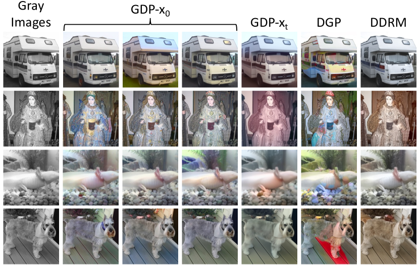
Figure 3: Qualitative comparison of colorization results on ImageNet validation images. GDP-$x_{0}$ generates various samples on the same input.

Unknown Degradation. In the real world, many images undergo complicated degradations [98], where the degradation models or the parameters of degradation models are unknown [86, 45]. In this case, the original images and the parameters of degradation models should be estimated simultaneously. For instance, in our work, the low-light image enhancement and the HDR recovery can be regarded as tasks with unknown degradation models. Here, we devise a simple but effective degradation model to simulate the complicated degradation, which can be formulated as follows:

$$\boldsymbol{y}=f\boldsymbol{x}+\boldsymbol{\mathcal{M}},$$ (10)

where the light factor $f$ is a scalar and the light mask $\boldsymbol{\mathcal{M}}$ is a vector of the same dimension as $\boldsymbol{x}$. $f$ and $\boldsymbol{\mathcal{M}}$ are unknown parameters of the degradation model. The reason that we can use this simple degradation model is that the transform between any pair of corrupted images and the corresponding high-quality image can be captured by $f$ and $\boldsymbol{\mathcal{M}}$ as long as they have the same size. If they do not have the same size, we can first resize $\boldsymbol{x}$ to the same size as $\boldsymbol{y}$ and then apply this transform. It is worth noting that this degradation model is non-linear in general, since $f$ and $\boldsymbol{\mathcal{M}}$ depend on $\boldsymbol{x}$ and $\boldsymbol{y}$. We need to estimate $f$ and $\boldsymbol{\mathcal{M}}$ for every individual corrupted image. We achieve this by randomly initializing them and synchronously optimizing them in the reverse process of DDPMs as shown in Algo.  2.

4.2 Extended version

Table 2: Quantitative comparison of linear image restoration tasks on ImageNet 1k [62]. GDP outperforms other methods in terms of FID and Consistency across all tasks.

Method	4$\times$ Super-resolution				Deblur				25$\%$ Inpainting				Colorization
	PSNR $\uparrow$	SSIM $\uparrow$	Consistency $\downarrow$	FID $\downarrow$	PSNR $\uparrow$	SSIM $\uparrow$	Consistency$\downarrow$	FID $\downarrow$	PSNR $\uparrow$	SSIM $\uparrow$	Consistency$\downarrow$	FID $\downarrow$	PSNR $\uparrow$	SSIM $\uparrow$	Consistency $\downarrow$	FID $\downarrow$
DGP [62]	21.65	0.56	158.74	152.85	26.00	0.54	475.10	136.53	27.59	0.82	414.60	60.65	18.42	0.71	305.59	94.59
SNIPS [33]	22.38	0.66	21.38	154.43	24.73	0.69	60.11	17.11	17.55	0.74	587.90	103.50	-	-	-	-
RED [69]	24.18	0.71	27.57	98.30	21.30	0.58	63.20	69.55	-	-	-	-	-	-	-	-
DDRM [32]	26.53	0.78	19.39	40.75	35.64	0.98	50.24	4.78	34.28	0.95	4.08	24.09	22.12	0.91	37.33	47.05
GDP-$x_{t}$	24.27	0.67	80.32	64.67	25.86	0.75	54.08	5.00	31.06	0.93	8.80	20.24	21.30	0.86	75.24	66.43
GDP-$x_{0}$	24.42	0.68	6.49	38.24	25.98	0.75	41.27	2.44	34.40	0.96	5.29	16.58	21.41	0.92	36.92	37.60

Table 3: Quantitative comparison of image enlighten task on LOL [88], VE-LOL-L [47], and LoLi-phone [41] benchmarks. Bold font indicates the best performance in zero-shot learning, and the underlined font denotes the best results in all models.

Learning	Methods	LOL [88]					VE-LOL-L [47]					LoLi-Phone [41]
		PSNR $\uparrow$	SSIM$\uparrow$	FID$\downarrow$	LOE$\downarrow$	PI$\downarrow$	PSNR$\uparrow$	SSIM$\uparrow$	FID $\downarrow$	LOE$\downarrow$	PI$\downarrow$	LOE$\downarrow$	PI$\downarrow$
Supervised learning	LLNet [50]	17.91	0.76	169.20	384.21	4.10	17.38	0.73	124.98	291.59	5.54	343.34	5.36
	LightenNet [43]	10.29	0.45	90.91	273.21	7.09	13.26	0.57	82.26	199.45	7.29	500.22	6.63
	Retinex-Net [88]	17.24	0.55	129.99	513.28	8.63	16.41	0.64	135.20	421.41	8.62	542.29	8.23
	MBLLEN [52]	17.90	0.77	122.69	175.10	8.39	15.95	0.70	105.74	114.91	7.45	137.34	6.46
	KinD [104]	17.57	0.82	74.52	377.59	7.41	18.07	0.78	80.12	253.79	7.51	265.47	6.84
	KinD++ [102]	17.60	0.80	100.15	712.12	7.96	16.80	0.74	101.23	421.97	7.98	382.51	7.71
	TBFEN [51]	17.25	0.83	90.59	367.66	8.29	18.91	0.81	91.30	276.65	8.02	214.30	7.34
	DSLR [46]	14.98	0.67	183.92	272.68	7.09	15.70	0.68	124.80	271.63	7.27	281.25	6.99
Unsupervised learning	EnlightenGAN [29]	17.44	0.74	82.60	379.23	8.78	17.45	0.75	86.51	311.85	8.27	373.41	7.26
Self-supervised learning	DRBN [92]	15.15	0.52	94.96	692.99	5.53	18.47	0.78	88.10	268.70	6.15	285.06	5.31
Zero-shot learning	ExCNet [99]	16.04	0.62	111.18	220.38	8.70	16.20	0.66	115.24	225.15	8.62	359.96	7.95
	Zero-DCE [23]	14.91	0.70	81.11	245.54	8.84	17.84	0.73	85.72	194.10	8.12	214.30	7.34
	Zero-DCE++ [42]	14.86	0.62	86.22	302.06	7.08	16.12	0.45	86.96	313.50	7.92	308.15	7.18
	RRDNet [106]	11.37	0.53	89.09	127.22	8.17	13.99	0.58	83.41	94.23	7.36	92.73	7.20
	GDP-$x_{t}$	7.32	0.57	238.92	364.15	8.26	9.45	0.50	152.68	194.49	7.12	508.73	8.06
	GDP-$x_{0}$	13.93	0.63	75.16	110.39	6.47	13.04	0.55	78.74	79.08	6.47	75.29	6.35

Multi-images Guidance. Under specific circumstances, there are several images could be utilized to guide the generation of a single image [59, 105], which is merely studied and much more challenging than single-image guidance. To this end, we propose the HDR-GDP for the HDR image recovery with multiple images as guidance, consisting of three input LDR images, i.e. short, medium, and long exposures. Similar to low-light enhancement, the degradation models are also treated as Eq. 10, where the parameters remain unknown that determine the HDR recovery is the blind problem. However, as shown in Fig. 2c and Algo. 5 in Appendix, in the reverse process, there are three corrupted images ($n$ = 3) to guide the generation so that three pairs of blind parameters for three LDR images are randomly initiated and optimized.

Figure 4: Qualitative results of (a) 25 $\%$ inpainting and (b) $4\times$ super-resolution on CelebA [31].

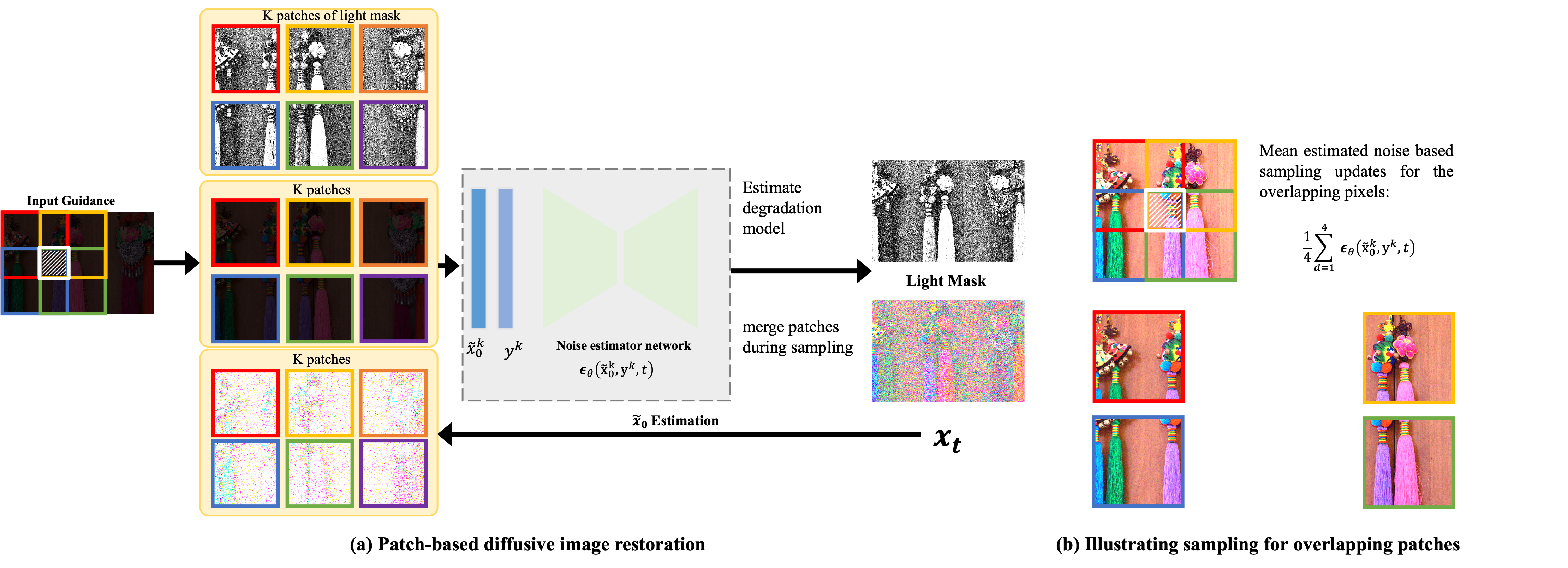
Figure 13: (a) Illustration of the patch-based image restoration pipeline detailed in Algorithm  6. (b) Illustrating mean estimated noise-guided sampling updates for overlapping pixels across patches. We demonstrate a simplified example where $r=p/2$, $r$ is the stride and $p$ is the patch size of images. And there are only four overlapping patches sharing the grid cell marked with the white border and gratings. The pixels in this region would be updated at each denoising step $t$ using the mean estimated noise over the four overlapping patches.

Restore Any-size Image. Furthermore, the pre-trained diffusion models provide by [15] with the size of 256 are only able to generate the fixed size of images, while the sizes of images from various image restoration are diverse. Herein, we employ the patch-based method as [47] to tackle this problem. By the merits of this patch-based strategy (Fig. 13 and Algo. 6 in the Appendix), GDP can be extended to recover the images of arbitrary resolution to promote the versatility of the GDP.

5 Loss Function

In GDP, the loss function can be divided into two main parts: Reconstruction loss and quality enhancement loss, where the former aims to recover the information contained in the conditional signal while the latter is integrated to promote the quality of the final outputs.

Reconstruction Loss. The reconstruction loss can be MSE, structural similarity index measure (SSIM), perceptual loss, or other reconstructive loss. Here, we primarily choose MSE loss as our reconstruction loss.

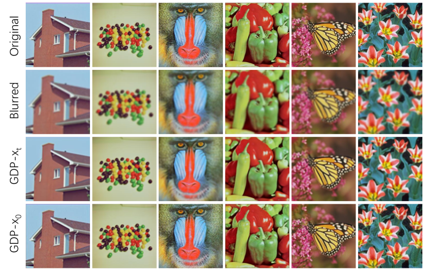
Figure 5: Results of image deblurring task on 256 $\times$ 256 USC-SIPI images [87] using an ImageNet model.

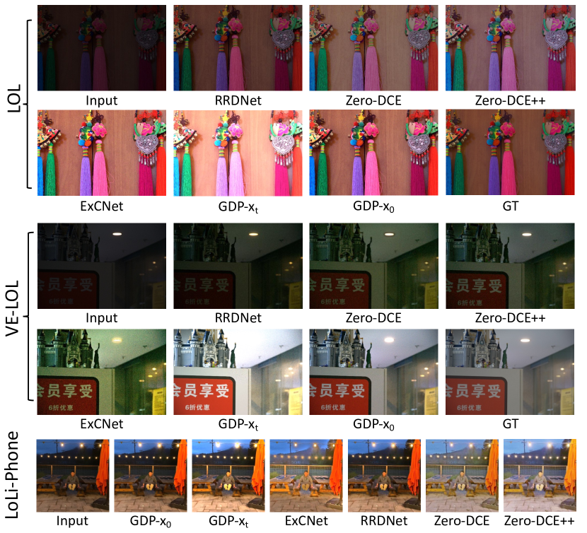
Figure 6: Qualitative results of low-light enhancement on the LOL [88], VE-LOL [47], and LoLi-Phone [41] datasets.

Quality Enhancement Loss. 1) Exposure Control Loss: To enhance the versatility of GDP , an exposure control loss $L_{exp}$ [23] is employed to control the exposure level for low-light image enhancement, which is written as:

$$\small L_{\text{exp}}=\frac{1}{U}\sum_{k=1}^{U}\left|R_{k}-E\right|,$$ (11)

where $U$ stands for the number of non-overlapping local regions of size $8\times 8$, and $R$ represents the average intensity value of a local region in the reconstructed image. Following the previous works [55, 56], $E$ is set as the gray level in the RGB color space. As expected, $E$ can be adjusted to control the brightness in our experiments.

2) Color Constancy Loss: Following the Gray-World color constancy hypothesis [6], a color constancy loss $L_{\text{col}}$ is exploited to correct the potential color deviations in the restored image and bridge the relations among the three adjusted channels in the colorization task, formulated as:

$$\footnotesize L_{\text{col}}=\sum_{\forall(m,n)\in\varepsilon}\left(Y^{m}-Y^{n}\right)^{2}\text{,}\varepsilon=\{(R,G),(R,B),(G,B)\}$$ (12)

where $Y^{m}$ is the average intensity value of $m$ channel in the recovered image, $(m,n)$ represents a pair of channels.

3) Illumination Smoothness Loss: To maintain the monotonicity relations between neighboring pixels in the optimized light mask $\mathcal{M}$, an illumination smoothness loss [23] is utilized for each light variance $\mathcal{M}$. The illumination smoothness loss $L_{tv_{\mathcal{M}}}$ is defined as:

$$\footnotesize L_{tv_{\mathcal{M}}}=\frac{1}{N}\sum_{n=1}^{N}\sum_{c\in\xi}\left(\left|\nabla_{h}\mathcal{M}_{n}^{c}\right|+\nabla_{v}\mathcal{M}_{n}^{c}\mid\right)^{2}\text{,}\xi=\{R,G,B\},$$ (13)

where $N$ is iteration times, $\nabla_{h}$ and $\nabla_{v}$ are the horizontal and vertical gradient operations, respectively.

Specifically, the image colorization task uses color constancy loss to obtain more natural colors. The low-light enhancement requires color constancy loss for the same reason. In addition, the low-light enhancement task uses illumination smoothness loss to make the estimated light mask $\boldsymbol{\mathcal{M}}$ smoother. Exposure control loss enables us to manually control the brightness of the restored image. The weights of the losses can be found in Appendix.

6 Experiments

In this section, we systematically compare GDP , which uses a single unconditional DDPM pre-trained on ImageNet provide by [15], with other methods of various image restoration and enhancement tasks, and ablate the effectiveness of the proposed design. We furthermore list details on implementation, datasets, evaluation, and more qualitative results for all tasks in Appendix.

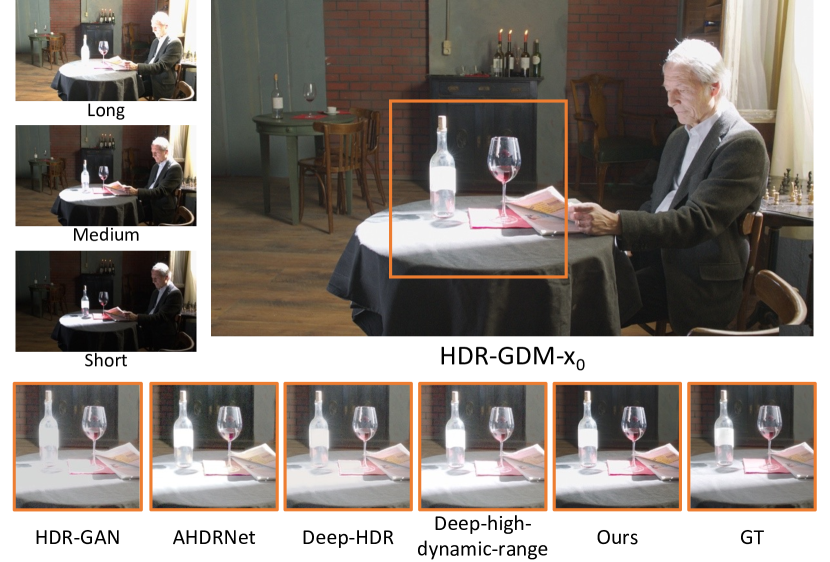
Figure 7: Example from the NTIRE dataset  [63]. We compare a set of patches cropped from the tone-mapped HDR images generated by state-of-the-art methods.

6.1 Linear and Multi-linear Degradation Tasks

Aiming at quantifying the performance of GDP, we focus on the ImageNet dataset for its diversity. For each experiment, we report the average peak signal-to-noise ratio (PSNR), SSIM, and Consistency to measure faithfulness to the original image and the FID to measure the resulting image quality. GDP is compared with other unsupervised methods that can operate on ImageNet, including RED [69], DGP [62], SNIPS [33], and DDRM [32]. We evaluate all methods on the tasks of $4\times$ super-resolution, deblurring, impainting, and colorization on one validation set from each of the $1000$ ImageNet classes, following [62]. Table 2 shows that GDP-$x_{0}$ outperforms other methods in Consistency and FID. The only exception is that DDRM achieves better PSNR and SSIM than GDP, but it requires higher Consistency and FID [15, 28, 73, 11, 13, 17]. GDP produces high-quality reconstructions across all the tested datasets and problems, which can be seen in Appendix. As a posterior sampling algorithm, GDP can produce multiple outputs for the same input, as demonstrated in the colorization task in Fig. 3. Moreover, the unconditional ImageNet DDPMs can be used to solve inverse problems on out-of-distribution images with general content. In Figs. 4 and 5, and more illustrations in Appendix, we show GDP successfully restores $256\times 256$ images from USC-SIPI [87], LSUN [94], and CelebA [31], which do not necessarily belong to any ImageNet class. GDP can also restore the images under multi-degradation (Fig. 1 and Appendix).

Table 4: Quantitative comparison on the NTIRE dataset [63].

Methods	PSNR$\uparrow$	SSIM$\uparrow$	LPIPS $\downarrow$	FID$\downarrow$
AHDRNet [91]	18.72	0.58	0.39	81.98
HDR-GAN [59]	21.67	0.74	0.26	52.71
Deep-HDR [90]	21.66	0.76	0.26	57.52
Deep-high-dyna mic-range [30]	21.33	0.71	0.26	51.92
GDP-$x_{t}$	19.36	0.65	0.30	63.89
GDP-$x_{0}$	24.88	0.86	0.13	50.05

6.2 Exposure Correction Tasks

Encouraged by the excellent performance on the linear inverse problem, we further evaluate our GDP on the low-light image enhancement, which is categorized into non-linear and blind issues. Following the previous works [41], the three datasets LOL [88], VE-LOL-L [47], and the most challenging LoLi-phone [41] are leveraged to test the capability of GDP on low-light enhancement. As shown in Table 3, our GDP-$x_{0}$ fulfills the best FID, lightness order error (LOE) [85], and perceptual index (PI) [57] across all the zero-shot methods under three datasets. The lower LOE demonstrates better preservation for the naturalness of lightness, while the lower PI indicates better perceptual quality. In Fig. 6 and Appendix, our GDP-$x_{0}$ yields the most reasonable and satisfactory results across all methods. For more control, by the merits of Exposure Control Loss, the brightness of the generated images can be adjusted by the well-exposedness level $E$ (Fig. 1 and Appendix)

6.3 HDR Image Recovery

To evaluate our model on the HDR recovery [41], we compare HDR-GDP-$x_{0}$ with the state-of-the-art HDR methods on the test images in the HDR dataset from the NTIRE2021 Multi-Frame HDR Challenge [63], from which we randomly select 100 different scenes as the validation. Each scene consists of three LDR images with various exposures and corresponding HDR ground truth. The state-of-the-art methods used for comparison include AHDRNet [91], HDR-GAN [59], DeepHDR [90] and deep-high-dynamic-range [30]. The quantitative results are provided in Table 4, where HDR-GDP-$x_{0}$ performs best in PSNR, SSIM, LPIPS, and FID. As shown in Fig. 7 and Appendix, HDR-GDP-$x_{0}$ achieves a better quality of reconstructed images, where the low-light parts can be enhanced, and the over-exposure regions are adjusted. Moreover, HDR-GDP-$x_{0}$ recovers the HDR images with more clear details.

6.4 Ablation Study

The Effectiveness of the Variance $\boldsymbol{\Sigma}$ and the Guidance Protocol. The ablation studies on the variance $\Sigma$ and two ways of guidance are performed to unveil their effectiveness. As shown in Table. 5, the performance of GDP-$x_{t}$ and GDP-$x_{0}$ is superior to GDP-$x_{t}$ with $\Sigma$ and GDP-$x_{0}$ with $\Sigma$, respectively, verifying the absence of variance $\Sigma$ can yield better quality of images. Moreover, the results of GDP-$x_{0}$ and GDP-$x_{0}$ with $\Sigma$ are better than GDP-$x_{t}$ and GDP-$x_{t}$ with $\Sigma$, respectively, demonstrating the superiority of the guidance on $\boldsymbol{x}_{0}$ protocol.

Table 5: The ablation study on the variance $\Sigma$ and the way of the guidance.

Task	4$\times$ Super resolution				Deblur
	PSNR	SSIM	Consistency	FID	PSNR	SSIM	Consistency	FID
GDP -$x_{t}$ with $\Sigma$	22.86	0.60	88.37	68.04	22.06	0.57	69.46	80.39
GDP -$x_{0}$ with $\Sigma$	22.09	0.58	93.19	41.22	23.49	0.65	68.67	50.29
GDP -$x_{t}$	24.27	0.67	80.32	64.67	25.86	0.73	54.08	5.00
GDP -$x_{0}$	24.42	0.68	6.49	38.24	25.98	0.75	41.27	2.44
Task	25$\%$ Inpainting				Colorization
	PSNR	SSIM	Consistency	FID	PSNR	SSIM	Consistency	FID
GDP -$x_{t}$ with $\Sigma$	25.28	0.70	171.44	73.32	17.67	0.70	246.26	145.20
GDP -$x_{0}$ with $\Sigma$	24.58	0.75	65.59	22.77	21.28	0.91	66.57	38.39
GDP -$x_{t}$	31.06	0.93	8.80	20.24	21.30	0.86	75.24	66.43
GDP -$x_{0}$	34.40	0.96	5.29	16.58	21.41	0.92	36.92	37.60

Table 6: The ablation study on the optimizable degradation and patch-based tactic.

Methods	LOL					NTIRE
	PSNR	SSIM	FID	LOE	PI	PSNR	SSIM	LPIPS	FID
Model A	11.05	0.49	156.51	707.57	8.61	24.12	0.67	0.32	86.69
Model B	9.01	0.37	355.99	969.89	9.04	9.83	0.04	1.02	253.11
GDP-$x_{t}$	7.32	0.57	238.92	364.15	8.26	19.36	0.65	0.30	63.89
GDP-$x_{0}$	13.93	0.63	75.16	110.39	6.47	24.88	0.86	0.13	50.05

The Effectiveness of the Trainable Degradation and the Patch-based Tactic. Moreover, to validate the influence of trainable parameters of the degradation model and our patch-based methods, further experiments are carried out on the LOL [88] and NTIRE [63] datasets. Model A is devised to naively restore the images from patches and patches where the parameters are not related. ModelB is designed with fixed parameters for all patches in the images. As shown in Table 6, our GDP-$x_{0}$ ranks first across all models and obtains the best visualization results (Fig. 7 and Appendix), revealing the strength of our proposed hierarchical guidance and patch-based method.

7 Conclusion

In this paper, we propose the Generative Diffusion Prior for unified image restoration that can be employed to tackle the linear inverse, non-linear and blind problems. Our GDP is able to restore any-size images via hierarchical guidance and patch-based methods. We systematically studied the way of guidance to exploit the strength of the DDPM. The GDP is comprehensively utilized on various tasks such as super-resolution, deblurring, inpainting, colorization, low-light enhancement, and HDR recovery, demonstrating the capabilities of GDP on unified image restoration.

Acknowledgement. This project is funded in part by Shanghai AI Laboratory

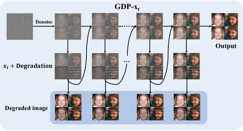
Figure 9: Overview of the GDP-$\boldsymbol{x}_{t}$. The guidance will be added on the noisy image $\boldsymbol{x}_{t}$ in every time step.

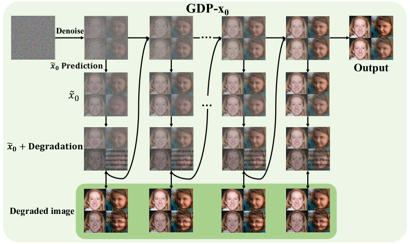
Figure 10: Overview of the GDP-$\boldsymbol{x}_{0}$. The guidance will be applied to a clean image $\tilde{\boldsymbol{x}}_{0}$ predicted from the noisy image $\boldsymbol{x}_{t}$.

Figure 11: Overview of the HDR-GDP-$\boldsymbol{x}_{0}$. The guidance will also be applied to a clean image $\tilde{\boldsymbol{x}}_{0}$. Unlike the GDP-$x_{0}$, three degraded images are utilized to guide the reverse process, and three sets of degradation models are optimized along the reverse process.

Input: Corrupted image $\boldsymbol{y}$, gradient scale $s$, degradation model $\mathcal{D}_{\phi}$ with randomly initiated parameters $\phi$, learning rate $l$ for optimizable degradation model, distance measure $\mathcal{L}$.

Output: Output image $\boldsymbol{x}_{0}$ conditioned on $\boldsymbol{y}$

Sample $\boldsymbol{x}_{T}$ from $\mathcal{N}(0,\mathbf{I})$

for $t$ from $T$ to 1 do

      

      $\mu,\Sigma=\mu_{\theta}\left(\boldsymbol{x}_{t}\right),\Sigma_{\theta}\left(\boldsymbol{x}_{t}\right)$

      $\mathcal{L}^{total}_{\phi,\boldsymbol{x}_{t}}=\mathcal{L}(\boldsymbol{y},{\mathcal{D}_{\phi}}\left(\boldsymbol{x}_{t}\right))+\mathcal{Q}\left(\boldsymbol{x}_{t}\right)$

      $\phi\leftarrow\phi-l\nabla_{\phi}\mathcal{L}^{total}_{\phi,\boldsymbol{x}_{t}}$

      Sample $\boldsymbol{x}_{t-1}$ by $\mathcal{N}\left(\mu+s\nabla_{\boldsymbol{{x}}_{t}}\mathcal{L}^{total}_{\phi,\boldsymbol{x}_{t}},\Sigma\right)$

end for

return $\boldsymbol{x}_{0}$

Algorithm 3 GDP-$\boldsymbol{x}_{t}$: Conditioner guided diffusion sampling on $\boldsymbol{x}_{t}$, given a diffusion model $\left(\mu_{\theta}\left(\boldsymbol{x}_{t}\right),\Sigma_{\theta}\left(\boldsymbol{x}_{t}\right)\right)$, corrupted image conditioner $\boldsymbol{y}$.

Input: Corrupted image $\boldsymbol{y}$, gradient scale $s$, degradation model $\mathcal{D}$, distance measure $\mathcal{L}$.

Output: Output image $\boldsymbol{x}_{0}$ conditioned on $\boldsymbol{y}$

Sample $\boldsymbol{x}_{T}$ from $\mathcal{N}(0,\mathbf{I})$

for $t$ from $T$ to 1 do

       $\mu,\Sigma=\mu_{\theta}\left(\boldsymbol{x}_{t}\right),\Sigma_{\theta}\left(\boldsymbol{x}_{t}\right)$

      $\boldsymbol{\tilde{x}}_{0}=\frac{\boldsymbol{x}_{t}}{\sqrt{\bar{\alpha}_{t}}}-\frac{\sqrt{1-\bar{\alpha}_{t}}\epsilon_{\theta}\left(\boldsymbol{x}_{t},t\right)}{\sqrt{\bar{\alpha}_{t}}}$

      $\mathcal{L}^{total}_{\boldsymbol{\tilde{x}}_{0}}=\mathcal{L}(\boldsymbol{y},{\mathcal{D}}\left(\boldsymbol{\tilde{x}}_{0}\right))+\mathcal{Q}\left(\boldsymbol{\tilde{x}}_{0}\right)$

      Sample $\boldsymbol{x}_{t-1}$ by $\mathcal{N}\left(\mu+s\nabla_{\boldsymbol{\tilde{x}}_{0}}\mathcal{L}^{total}_{\boldsymbol{\tilde{x}}_{0}},\Sigma\right)$

end for

return $\boldsymbol{x}_{0}$

Algorithm 4 GDP-$\boldsymbol{x}_{0}$: Conditioner guided diffusion sampling on $\boldsymbol{\tilde{x}}_{0}$, given a diffusion model $\left(\mu_{\theta}\left(\boldsymbol{x}_{t}\right),\Sigma_{\theta}\left(\boldsymbol{x}_{t}\right)\right)$, corrupted image conditioner $\boldsymbol{y}$.

Input: Corrupted image $\{\boldsymbol{y}^{i}\mid i=1,2,\ldots,n\}$ ($n$ = 3 for HDR recovery (LDR-long image $\boldsymbol{y}^{1}$, LDR-medium image $\boldsymbol{y}^{2}$, LDR-short image $\boldsymbol{y}^{3}$) and $n$ = 1 for other tasks), gradient scale $s$, degradation models $\{\mathcal{D}_{\phi^{i}}|i=1,2,\dots,n\}$ with randomly initiated parameters $\{{\phi^{i}}|i=1,2,\dots,n\}$, learning rate $l$ for optimizable degradation model, distance measure $\mathcal{L}$.

Output: Output image $\boldsymbol{x}_{0}$ conditioned on $\{\boldsymbol{y}^{i}\mid i=1,2,\ldots,n\}$

Sample $\boldsymbol{x}_{T}$ from $\mathcal{N}(0,\mathbf{I})$

for $t$ from $T$ to 1 do

       $\mu,\Sigma=\mu_{\theta}\left(\boldsymbol{x}_{t}\right),\Sigma_{\theta}\left(\boldsymbol{x}_{t}\right)$

      $\boldsymbol{\tilde{x}}_{0}=\frac{\boldsymbol{x}_{t}}{\sqrt{\bar{\alpha}_{t}}}-\frac{\sqrt{1-\bar{\alpha}_{t}}\epsilon_{\theta}\left(\boldsymbol{x}_{t},t\right)}{\sqrt{\bar{\alpha}_{t}}}$

      $\mathcal{L}^{total}_{\phi,\boldsymbol{\tilde{x}}_{0}}=0$

      for $j$ from 1 to n do

            

            $\mathcal{L}_{{\phi^{j}},\boldsymbol{\tilde{x}}_{0}}=\mathcal{L}(\boldsymbol{y}^{j},{\mathcal{D}_{\phi^{j}}}\left(\boldsymbol{\tilde{x}}_{0}\right))+\mathcal{Q}\left(\boldsymbol{\tilde{x}}_{0}\right)$

            ${\phi^{j}}={\phi^{j}}-l\nabla_{{\phi^{j}}}\mathcal{L}_{{\phi^{j}},\boldsymbol{\tilde{x}}_{0}}$

            $\mathcal{L}^{total}_{\phi,\boldsymbol{\tilde{x}}_{0}}=\mathcal{L}^{total}_{\phi,\boldsymbol{\tilde{x}}_{0}}+\mathcal{L}_{\phi^{j},\boldsymbol{\tilde{x}}_{0}}$

       end for

      

      Sample $\boldsymbol{x}_{t-1}$ by $\mathcal{N}\left(\mu+s\nabla_{\boldsymbol{\tilde{x}}_{0}}\mathcal{L}^{total}_{\phi,\boldsymbol{\tilde{x}}_{0}},\Sigma\right)$

end for

return $\boldsymbol{x}_{0}$

Algorithm 5 GDP-$\boldsymbol{x}_{0}$: Conditioner guided diffusion sampling on $\boldsymbol{x}_{0}$, given a diffusion model $\left(\mu_{\theta}\left(\boldsymbol{x}_{t}\right),\Sigma_{\theta}\left(\boldsymbol{x}_{t}\right)\right)$, corrupted images conditioner $\{\boldsymbol{y}^{i}\mid i=1,2,\ldots,n\}$.

Input: Conditioner guided diffusion sampling on $\boldsymbol{\tilde{x}}_{0}$, given a diffusion model $\left(\mu_{\theta}\left(\boldsymbol{x}_{t}\right),\Sigma_{\theta}\left(\boldsymbol{x}_{t}\right)\right)$, corrupted image conditioner $\boldsymbol{y}$, degradation model $\mathcal{D}_{\phi}:\boldsymbol{y}=f\boldsymbol{x}+\boldsymbol{\mathcal{M}}$ with randomly initiated parameters $\phi$, learning rate $l$ for optimizable degradation model. Dictionary of $K$ overlapping patch locations, and a binary patch mask $\mathbf{P}^{k}$.

Output: Output image $\boldsymbol{x}_{0}$ conditioned on $\boldsymbol{y}$

Sample $\boldsymbol{x}_{T}$ from $\mathcal{N}(0,\mathbf{I})$

for $t$ from $T$ to 1 do

      

      $\mu,\Sigma=\mu_{\theta}\left(\boldsymbol{x}_{t}\right),\Sigma_{\theta}\left(\boldsymbol{x}_{t}\right)$

      $\text{Mean vector }\boldsymbol{\Omega}_{t}=\mathbf{0}\text{ and variance vector }\boldsymbol{\psi}_{t}=\mathbf{0}\text{ and weight vector }\mathbf{G}=\mathbf{0}\text{ and }f=\mathbf{0}\text{ and }\boldsymbol{\mathcal{M}}=\mathbf{0}$

      for $k=1,\ldots,K$ do

             $\boldsymbol{x}_{t}^{k}=\operatorname{Crop}\left(\mathbf{P}^{k}\circ\boldsymbol{x}_{t}\right)$

            $\boldsymbol{y}^{k}=\operatorname{Crop}\left(\mathbf{P}^{k}\circ\boldsymbol{y}\right)$

            $\boldsymbol{\mathcal{M}}^{k}=\operatorname{Crop}\left(\mathbf{P}^{k}\circ\boldsymbol{\mathcal{M}}\right)$

            $\boldsymbol{\tilde{x}}_{0}^{k}=\frac{\boldsymbol{x}_{t}^{k}}{\sqrt{\bar{\alpha}_{t}}}-\frac{\sqrt{1-\bar{\alpha}_{t}}\epsilon_{\theta}\left(\boldsymbol{x}_{t}^{k},t\right)}{\sqrt{\bar{\alpha}_{t}}}$

            $\mathcal{L}^{total}_{\phi,\boldsymbol{\tilde{x}}_{0}^{k}}=\mathcal{L}(\boldsymbol{y}^{k},{\mathcal{D}_{\phi}}\left(\boldsymbol{\tilde{x}}_{0}^{k}\right))+\mathcal{Q}\left(\boldsymbol{\tilde{x}}_{0}^{k}\right)$

            $f^{k}\leftarrow f^{k}-l\nabla_{f^{k}}\mathcal{L}^{total}_{f^{k},\boldsymbol{\tilde{x}}_{0}^{k}}$

            $\boldsymbol{\mathcal{M}}^{k}\leftarrow\boldsymbol{\mathcal{M}}^{k}-l\nabla_{\boldsymbol{\mathcal{M}}^{k}}\mathcal{L}^{total}_{\boldsymbol{\mathcal{M}}^{k},\boldsymbol{\tilde{x}}_{0}^{k}}$

            $\mu^{k}=\mu+s\nabla_{\boldsymbol{\tilde{x}}_{0}^{k}}\mathcal{L}^{total}_{\phi,\boldsymbol{\tilde{x}}_{0}^{k}}$

            $f=f+f^{k}$

            $\boldsymbol{\Omega}_{t}=\mathbf{\Omega}_{t}+\mathbf{P}_{k}\cdot\mu^{k}$

            $\boldsymbol{\psi}_{t}=\mathbf{\psi}_{t}+\mathbf{P}^{k}\cdot\sigma^{k}$

            $\boldsymbol{\mathcal{M}}=\boldsymbol{\mathcal{M}}+\mathbf{P}^{k}\cdot\boldsymbol{\mathcal{M}}^{k}$

            $\mathbf{G}=\mathbf{G}+\mathbf{P}^{k}$

       end for

      

      $\mathbf{\Omega}_{t}=\mathbf{\Omega}_{t}\oslash\mathbf{G}\quad\quad//\oslash:\text{ element-wise division }$

      $\mathbf{\psi}_{t}=\mathbf{\psi}_{t}\oslash\mathbf{G}$

      $\boldsymbol{\mathcal{M}}=\boldsymbol{\mathcal{M}}\oslash\mathbf{G}$

      $f=f/K$

      Sample $\boldsymbol{x}_{t-1}$ by $\mathcal{N}\left(\mathbf{\Omega}_{t},\mathbf{\psi}_{t}\right)$

end for

return Restored any-size image $\boldsymbol{x}_{0}$

Algorithm 6 Restore Any-size Image

Appendix A Limitations and Future works

Limitations. The main limitation of our work is its inference time. Since we might add several guidance steps in every time step $t$, the sampling time is extended. This limits the applicability of our method to real-time applications and weak end-user devices such as mobile devices. To address this issue, further research into accelerated diffusion sampling techniques is required.

In addition, the choice of the guidance scale is also obtained through experiments, which means that for samples with different distributions, it is necessary to manually select the optimal guidance scale. However, we found that for the same distribution of data, an approximate degradation model may lead to close guidance scales. This phenomenon may be proved mathematically in future work.

Future works. In future work, in addition to further optimizing the time step and variance schedules, it would be interesting to investigate the following:

(i) The Guided Diffusion Prior can also theoretically be applied to 3D data restoration. For instance, point cloud completion and upsampling can be regarded as linear inverse problems in 3D vision. Shapeinversion [97] tackles the point cloud completion by GAN inversion, where the GDP can hopefully be integrated.

(ii) Moreover, since LiDAR is affected by various kinds of weather in the real world and also produces various non-linear degradations, GDP should also be explored for the recovery of these point clouds.

(iii) Self-supervised training techniques inspired by our GDP and techniques used in supervised techniques [72] that further improve the performance of unsupervised image restoration models.

Appendix B Implementation Details

We apply GDP to a suite of challenging image restoration tasks: (1) Colorization transforms an input gray-scale image to a plausible color image. (2) Inpainting fills in user-specified masked regions of an image with realistic content. (3) Super-resolution extends a low-resolution image into a higher one. (4) Deblurring corrects the blurred images, restoring plausible image detail. (5) Enlighting enables the dark images turned into normal images. (6) HDR image recovery aims to obtain HDR images with the aid of three LDR images. Inputs and outputs of the first four tasks are represented as $256\times 256$ RGB images, while the last two tasks are various ($1900\times 1060$ for HDR image recovery and $600\times 400$ for image enlightening, respectively). We do so without task-specific hyperparameter tuning and architecture customization.

Colorization requires the representation of objects, segmentation, and layouts with long-range image dependencies. Inpainting is challenging due to large masks, image diversity, and cluttered scenes. Super-resolution and deblurring are also not trivial because the degradation might damage the content of the images. While the other tasks are linear in nature, low-light enhancement and HDR recovery are non-linear inverse problems; they require a good model of natural image statistics to detect and correct over-exposed and under-exposed areas. Although previous works have studied these problems extensively, it is rare that a model with no task-specific engineering achieves strong performance in all tasks, beating strong task-specific GAN and regression baselines. Our GDP is devised to achieve this goal.

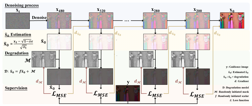
Figure 12: Illustration of the patch-based method for any-size image restoration.

B.1 Dataset briefs

ImageNet, LSUN, CelebA, and USC-SIPI Datasets. To quantitatively evaluate GDP on linear image restoration tasks, we test on 1k images from the ImageNet validation set following [62]. The CelebA-HQ [40] dataset is a high-quality subset of the Large-Scale CelebFaces Attributes (CelebA) dataset [49]. LSUN dataset [94] contains around one million labeled images for each of 10 scene categories and 20 object categories. And the USC-SIPI dataset [87] is a collection of various digitized images. We utilize the images from CelebA, LSUN, and USC-SIPI provided by [32].

LOL Dataset. The LOL dataset [88] is composed of 500 low-light and normal-light image pairs and divided into 485 training pairs and 15 testing pairs. The low-light images contain noise produced during the photo capture process. Most of the images are indoor scenes. All the images have a resolution of 400 $\times$ 600.

VE-LOL-L Dataset. For underexposure correction experiments, we use the paired data of the VE-LOL-L dataset [47], in which each captured well-exposed image has its underexposed version with different underexposure levels. Note that the VE-LOL-L dataset, consisting of VE-LOL-Cap and VE-LOL-Syn, is also carried out. Due to the different distribution of the two sub-set, we solve them under different guidance scales.

LoLi-Phone Dataset. LoLi-Phone [41] is a large-scale low-light image and video dataset for low-light image enhancement. The images and videos are taken by different mobile phone cameras under diverse illumination conditions.

NTIRE Dataset [64]. In the NTIRE dataset, there are 1494 LDRs/HDR for training, 60 images for validation, and 201 images for testing. The 1494 frames consist of 26 long shots. Each scene contains three LDR images, their corresponding exposure and alignment information, and HDR ground truth. The size of an image is $1060\times 1900$. Since the ground truth of the validation and test sets are not available, we only do experiments on the training set. We select 100 images as the test set.

B.2 Experimental Setup

In each inverse problem, the pixel values are in the range [0,1], and the resulting degradation measures are as follows: (i) For super-resolution, a block averaging filter is utilized to downscale the image on each axis 4 times; (ii) In terms of deblurring, the image is blurred by a 9$\times 9$ unified kernel. (iii) For colorization, the gray-scale image is the average of the red, green, and blue channels of the original image; (iv) For inpainting, we cover parts of the original image with text overlays or randomly delete 25$\%$ pixels.

In the non-linear and blind problem, the images from the low-light dataset and NTIRE dataset are naturally over-exposed or under-exposed. Therefore, no additional operations are required for the images.

Appendix C Evaluation Metrics

Apart from the commonly used PSNR and SSIM, other metrics are also utilized for evaluation: (i) FID [26] is an objective metric used to assess the quality of synthesized images. (ii) Consistency [73] measures MSE between the degraded inputs and the outputs undergoing the same degradation. (iii) Learned perceptual image patch similarity (LPIPS) [101] is also adopted, a deep feature-based perceptual distance metric to further assess the image quality. (iv) The non-reference perceptual index (PI) [57] is also employed to evaluate perceptual quality. The PI metric is originally utilized to measure perceptual quality in image super-resolution. It has also been used to assess the performance of other image restoration tasks. A lower PI value indicates better perceptual quality. (v) The lightness order error (LOE) [85] is employed as our objective metric to measure the performance. The definition of LOE is as follows:

$$LOE=\frac{1}{m}\sum_{x=1}^{m}\sum_{y=1}^{m}\left(U(\mathbf{T}(x),\mathbf{T}(y))\oplus U\left(\mathbf{T}_{r}(x),\mathbf{T}_{r}(y)\right)\right)$$ (14)

where $m$ is the pixel number. The function $U(p,q)$ returns 1 if $p>=q,0$ otherwise. $\oplus$ stands for the exclusive-or operator. In addition, $\mathbf{T}(x)$ and $\mathbf{T}_{r}(x)$ are the maximum values among $\mathrm{R},\mathrm{G}$ and $\mathrm{B}$ channels at location $x$ of the enhanced and reference images, respectively. The lower the LOE is, the better the enhancement preserves the naturalness of lightness.

Appendix D Further elaboration of the models

GDP-$\boldsymbol{x}_{t}$. As shown in Fig. 9, the guidance is conditioned on $\boldsymbol{x}_{t}$ but with the absence of $\Sigma$. The noisy images are gradually denoised during the reverse process. And the $\boldsymbol{x}_{t}$ undergoing the degradation model is more similar to the corrupted image. The gradients $\nabla$ of the loss function are utilized to control the mean of the conditional distribution.

GDP-$\boldsymbol{x}_{0}$. To make a clear comparison, we also illustrate the GDP-$\boldsymbol{x}_{0}$ in Fig. 10, and Algorithm 2 in the main paper. Different from the GDP-$\boldsymbol{x}_{t}$, GDP-$\boldsymbol{x}_{0}$ will predict the intermediate variance $\boldsymbol{\tilde{x}}_{0}$ from the noisy image $\boldsymbol{x}_{t}$ by estimating the noise in $\boldsymbol{x}_{t}$, which can be directly inferred when given the $\boldsymbol{x}_{t}$ in every time steps $t$. Then the predicted $\boldsymbol{\tilde{x}}_{0}$ goes through the same degradation as input to obtain $\boldsymbol{\hat{x}}_{0}$. Note that the degradation might be unknown. Then the loss between the $\boldsymbol{\hat{x}}_{0}$ and the corrupted image $\boldsymbol{y}$, the gradients will be applied to optimize the unknown degradation models and sample the next step latent $\boldsymbol{x}_{t-1}$.

HDR-GDP-$\boldsymbol{x}_{0}$. As depicted in Fig. 11, and Algorithm 5, there are three images to guide the reverse process. As a blind problem, we randomly initiate three sets of the parameters of the degradation models. At every time step, $\boldsymbol{\tilde{x}}_{0}$ will undergo the three degradation models $\mathcal{D}^{i}$, respectively. Unlike GDP-$\boldsymbol{x}_{0}$, the gradients of the three losses are used to optimize the corresponding degradation model and all leveraged to sample the next step latent $\boldsymbol{x}_{t-1}$.

Hierarchical Guidance and Patch-based Methods. As vividly illustrated in Fig. 12 and  13, we resize the corrupted images $\boldsymbol{y}\in\mathbb{R}^{3\times H\times W}$ to $\boldsymbol{\overline{y}}\in\mathbb{R}^{3\times 256\times\overline{W}\text{ or }3\times\overline{H}\times 256}$, then apply the patch-based methods [61] on the reshaped images. Following that, the light masks $\boldsymbol{\mathcal{\overline{M}}}$ are interpolated to the original image size to obtain the $\boldsymbol{\mathcal{M}}$, which can be regarded as the global light shift. After, the light factor $\boldsymbol{f}$ and the light mask $\boldsymbol{\mathcal{M}}$ will be fixed and utilized to generate the image patches of the original images, which will be finally recombined as the output images. In our experiments, low-light enhancement and HDR recovery problems can be tackled by this strategy.

Table 7: The guidance scales and the number of optimization per time step on the various tasks. Note that these parameters may not be optimal due to the infinite number of possible combinations.

Tasks	Dataset	Guidance scale	The number of optimization per time step
4$\times$ Super-resolution	ImageNet [62]	2E+03	6
Deblurring	ImageNet [62]	6E+03	6
25$\%$ Inpainting	ImageNet [62]	4E+03	6
Colorization	ImageNet [62]	6E+03	6
Low-light enhancement	LOL dataset [88]	1E+05	6
HDR recovery	NTIRE dataset [64]	1E+05	1

Appendix E Further Ablation Study on the Guidance

To gain insight into the way of guidance, apart from GDP-$\boldsymbol{x}_{t}$ and GDP-$\boldsymbol{x}_{0}$, two more variants GDP-$\boldsymbol{x}_{t}$-v1 and GDP-$\boldsymbol{x}_{0}$-v1 are devised for comparison.

The main difference among these four variants is the way of mean shift. The mean shift of four variants can be written as follow:

$$\text{GDP-}\boldsymbol{x}_{0}:\tilde{\boldsymbol{\mu}}_{t}\left(\boldsymbol{x}_{t},\boldsymbol{\tilde{x}}_{0}\right)=$$ (15)

$$\frac{\sqrt{\bar{\alpha}_{t-1}}\beta_{t}}{1-\bar{\alpha}_{t}}\boldsymbol{\tilde{x}}_{0}+\frac{\sqrt{\alpha_{t}}\left(1-\bar{\alpha}_{t-1}\right)}{1-\bar{\alpha}_{t}}\boldsymbol{x}_{t}+s\nabla_{\boldsymbol{\tilde{x}}_{0}}\mathcal{L}^{total}_{\boldsymbol{\tilde{x}}_{0}}$$

$$\text{GDP-}\boldsymbol{x}_{t}:\tilde{\boldsymbol{\mu}}_{t}\left(\boldsymbol{x}_{t},\boldsymbol{\tilde{x}}_{0}\right)=$$

$$\frac{\sqrt{\bar{\alpha}_{t-1}}\beta_{t}}{1-\bar{\alpha}_{t}}\boldsymbol{\tilde{x}}_{0}+\frac{\sqrt{\alpha_{t}}\left(1-\bar{\alpha}_{t-1}\right)}{1-\bar{\alpha}_{t}}\boldsymbol{x}_{t}+s\nabla_{\boldsymbol{x}_{t}}\mathcal{L}^{total}_{\boldsymbol{x}_{t}}$$

$$\text{GDP-}\boldsymbol{x}_{0}\text{-v1}:\tilde{\boldsymbol{\mu}}_{t}\left(\boldsymbol{x}_{t},\boldsymbol{\tilde{x}}_{0}\right)=$$

$$\frac{\sqrt{\bar{\alpha}_{t-1}}\beta_{t}}{1-\bar{\alpha}_{t}}(\boldsymbol{\tilde{x}}_{0}+s\nabla_{\boldsymbol{\tilde{x}}_{0}}\mathcal{L}^{total}_{\boldsymbol{\tilde{x}}_{0}})+\frac{\sqrt{\alpha_{t}}\left(1-\bar{\alpha}_{t-1}\right)}{1-\bar{\alpha}_{t}}\boldsymbol{x}_{t}$$

$$\text{GDP-}\boldsymbol{x}_{t}\text{-v1}:\tilde{\boldsymbol{\mu}}_{t}\left(\boldsymbol{x}_{t},\boldsymbol{\tilde{x}}_{0}\right)=$$

$$\frac{\sqrt{\bar{\alpha}_{t-1}}\beta_{t}}{1-\bar{\alpha}_{t}}\boldsymbol{\tilde{x}}_{0}+\frac{\sqrt{\alpha_{t}}\left(1-\bar{\alpha}_{t-1}\right)}{1-\bar{\alpha}_{t}}(\boldsymbol{x}_{t}+s\nabla_{\boldsymbol{x}_{t}}\mathcal{L}^{total}_{\boldsymbol{x}_{t}}).$$

where GDP-$\boldsymbol{x}_{0}$ directly add the mean shift $s\nabla_{\boldsymbol{x}_{0}}\mathcal{L}^{total}_{\boldsymbol{x}_{0}}$ into $\tilde{\boldsymbol{\mu}}_{t}\left(\boldsymbol{x}_{t},\boldsymbol{\tilde{x}}_{0}\right)$ without the coefficient $\frac{\sqrt{\bar{\alpha}_{t-1}}\beta_{t}}{1-\bar{\alpha}_{t}}$, compared with GDP-$\boldsymbol{x}_{0}$-v1.

It is experimentally found that GDP-$\boldsymbol{x}_{0}$ and GDP-$\boldsymbol{x}_{t}$ fulfills better performance on four linear tasks than GDP-$\boldsymbol{x}_{0}$-v1 and GDP-$\boldsymbol{x}_{t}$-v1 in Table. 8.

Table 8: The performance of ablation studies on the way of guidance. We compare four ways of guidance in terms of FID.

FID	4x super-resolution	Deblur	25$\%$ Inpainting	Colorization
GDP-$\boldsymbol{x}_{t}$-v1	108.06	88.52	113.47	102.37
GDP-$\boldsymbol{x}_{0}$-v1	44.16	10.35	37.32	41.53
GDP-$\boldsymbol{x}_{t}$	64.67	5.00	20.24	66.43
GDP-$\boldsymbol{x}_{0}$	38.24	2.44	16.58	37.60

Input: Corrupted image $\boldsymbol{y}$, gradient scale $s$, degradation model $\mathcal{D}$, distance measure $\mathcal{L}$, optional quality enhancement loss $\mathcal{Q}$, quality enhancement scale $\lambda$.

Output: Output image $\boldsymbol{x}_{0}$ conditioned on $\boldsymbol{y}$

Sample $\boldsymbol{x}_{T}$ from $\mathcal{N}(0,\mathbf{I})$

for $t$ from $T$ to 1 do

       $\mu,\Sigma=\mu_{\theta}\left(\boldsymbol{x}_{t}\right),\Sigma_{\theta}\left(\boldsymbol{x}_{t}\right)$

      $\boldsymbol{\tilde{x}}_{0}=\frac{\boldsymbol{x}_{t}}{\sqrt{\bar{\alpha}_{t}}}-\frac{\sqrt{1-\bar{\alpha}_{t}}\epsilon_{\theta}\left(\boldsymbol{x}_{t},t\right)}{\sqrt{\bar{\alpha}_{t}}}$

      $\mathcal{L}^{total}_{\boldsymbol{{x}}_{t}}=\mathcal{L}(\boldsymbol{y},{\mathcal{D}}\left(\boldsymbol{{x}}_{t}\right))+\mathcal{Q}\left(\boldsymbol{{x}}_{t}\right)$

      $\boldsymbol{{x}}_{t}\leftarrow\boldsymbol{x}_{t}-s\nabla_{\boldsymbol{{x}}_{t}}\mathcal{L}\left(\boldsymbol{y},{\mathcal{D}}\left(\boldsymbol{x_{t}}\right)\right)$

      Sample $\boldsymbol{x}_{t-1}$ by $q\left(\boldsymbol{x}_{t-1}\mid\boldsymbol{x}_{t},\boldsymbol{\tilde{x}}_{0}\right)=\mathcal{N}\left(\boldsymbol{x}_{t-1};\tilde{\boldsymbol{\mu}}_{t}\left(\boldsymbol{x}_{t},\boldsymbol{\tilde{x}}_{0}\right),\tilde{\beta}_{t}\mathbf{I}\right)$,

      where $\quad\tilde{\boldsymbol{\mu}}_{t}\left(\boldsymbol{x}_{t},\boldsymbol{\tilde{x}}_{0}\right)=\frac{\sqrt{\bar{\alpha}_{t-1}}\beta_{t}}{1-\bar{\alpha}_{t}}\boldsymbol{\tilde{x}}_{0}+\frac{\sqrt{\alpha_{t}}\left(1-\bar{\alpha}_{t-1}\right)}{1-\bar{\alpha}_{t}}\boldsymbol{x}_{t}\quad$ and $\quad\tilde{\beta}_{t}=\frac{1-\bar{\alpha}_{t-1}}{1-\bar{\alpha}_{t}}\beta_{t}$

end for

return $\boldsymbol{x}_{0}$

Algorithm 7 GDP-$\boldsymbol{x}_{t}$-v1 with fixed degradation model: Conditioner guided diffusion sampling on $\boldsymbol{x}_{t}$, given a diffusion model $\left(\mu_{\theta}\left(\boldsymbol{x}_{t}\right),\Sigma_{\theta}\left(\boldsymbol{x}_{t}\right)\right)$, corrupted image conditioner $\boldsymbol{y}$.

Input: Corrupted image $\boldsymbol{y}$, gradient scale $s$, degradation model $\mathcal{D}$, distance measure $\mathcal{L}$.

Output: Output image $\boldsymbol{x}_{0}$ conditioned on $\boldsymbol{y}$

Sample $\boldsymbol{x}_{T}$ from $\mathcal{N}(0,\mathbf{I})$

for $t$ from $T$ to 1 do

       $\mu,\Sigma=\mu_{\theta}\left(\boldsymbol{x}_{t}\right),\Sigma_{\theta}\left(\boldsymbol{x}_{t}\right)$

      $\boldsymbol{\tilde{x}}_{0}=\frac{\boldsymbol{x}_{t}}{\sqrt{\bar{\alpha}_{t}}}-\frac{\sqrt{1-\bar{\alpha}_{t}}\epsilon_{\theta}\left(\boldsymbol{x}_{t},t\right)}{\sqrt{\bar{\alpha}_{t}}}$

      $\mathcal{L}^{total}_{\boldsymbol{\tilde{x}}_{0}}=\mathcal{L}(\boldsymbol{y},{\mathcal{D}}\left(\boldsymbol{\tilde{x}}_{0}\right))+\mathcal{Q}\left(\boldsymbol{\tilde{x}}_{0}\right)$

      $\boldsymbol{\tilde{x}}_{0}\leftarrow\boldsymbol{\tilde{x}}_{0}-s\nabla_{\boldsymbol{\tilde{x}}_{0}}\mathcal{L}^{total}_{\boldsymbol{\tilde{x}}_{0}}$

      Sample $\boldsymbol{x}_{t-1}$ by $q\left(\boldsymbol{x}_{t-1}\mid\boldsymbol{x}_{t},\boldsymbol{\tilde{x}}_{0}\right)=\mathcal{N}\left(\boldsymbol{x}_{t-1};\tilde{\boldsymbol{\mu}}_{t}\left(\boldsymbol{x}_{t},\boldsymbol{\tilde{x}}_{0}\right),\tilde{\beta}_{t}\mathbf{I}\right)$,

      where $\quad\tilde{\boldsymbol{\mu}}_{t}\left(\boldsymbol{x}_{t},\boldsymbol{\tilde{x}}_{0}\right)=\frac{\sqrt{\bar{\alpha}_{t-1}}\beta_{t}}{1-\bar{\alpha}_{t}}\boldsymbol{\tilde{x}}_{0}+\frac{\sqrt{\alpha_{t}}\left(1-\bar{\alpha}_{t-1}\right)}{1-\bar{\alpha}_{t}}\boldsymbol{x}_{t}\quad$ and $\quad\tilde{\beta}_{t}=\frac{1-\bar{\alpha}_{t-1}}{1-\bar{\alpha}_{t}}\beta_{t}$

end for

return $\boldsymbol{x}_{0}$

Algorithm 8 GDP-$\boldsymbol{x}_{0}$-v1: Conditioner guided diffusion sampling on $\boldsymbol{\tilde{x}}_{0}$, given a diffusion model $\left(\mu_{\theta}\left(\boldsymbol{x}_{t}\right),\Sigma_{\theta}\left(\boldsymbol{x}_{t}\right)\right)$, corrupted image conditioner $\boldsymbol{y}$.

Appendix F The ELBO objective of GDP

GDP is a Markov chain conditioned on $\boldsymbol{y}$, resulting in the following ELBO objective [77]:

$$\mathbb{E}_{\boldsymbol{x}_{0}\sim q\left(\boldsymbol{x}_{0}\right),\boldsymbol{y}\sim q\left(\boldsymbol{y}\mid\boldsymbol{x}_{0}\right)}\left[\log p_{\theta}\left(\boldsymbol{x}_{0}\mid\boldsymbol{y}\right)\right]\geq$$ (16)

$$-\mathbb{E}\left[\sum_{t=1}^{T-1}{\mathrm{KL}}\left(q^{t}\left(\boldsymbol{x}_{t}\mid\boldsymbol{x}_{t+1},\boldsymbol{x}_{0},\boldsymbol{y}\right)\|p_{\theta}^{t}\left(\boldsymbol{x}_{t}\mid\boldsymbol{x}_{t+1},\boldsymbol{y}\right)\right)\right]$$

$$+\mathbb{E}\left[\log p_{\theta}^{0}\left(\boldsymbol{x}_{0}\mid\boldsymbol{x}_{1},\boldsymbol{y}\right)\right]$$

$$-\mathbb{E}\left[{\mathrm{KL}}\left(q^{T}\left(\boldsymbol{x}_{T}\mid\boldsymbol{x}_{0},\boldsymbol{y}\right)\|p_{\theta}^{T}\left(\boldsymbol{x}_{T}\mid\boldsymbol{y}\right)\right)\right]$$

where $q\left(\boldsymbol{x}_{0}\right)$ denotes the data distribution, $q\left(\boldsymbol{y}\mid\boldsymbol{x}_{0}\right)$ in the main paper, the expectation on the right-hand side is given by sampling $\boldsymbol{x}_{0}\sim q\left(\boldsymbol{x}_{0}\right),\boldsymbol{y}\sim q\left(\boldsymbol{y}\mid\boldsymbol{x}_{0}\right),\boldsymbol{x}_{T}\sim q^{T}\left(\boldsymbol{x}_{T}\mid\boldsymbol{x}_{0},\boldsymbol{y}\right)$, and $\boldsymbol{x}_{t}\sim q^{t}\left(\boldsymbol{x}_{t}\mid\boldsymbol{x}_{t+1},\boldsymbol{x}_{0},\boldsymbol{y}\right)$ for $t\in[1,T-1]$.

Appendix G Sampling with DDIM

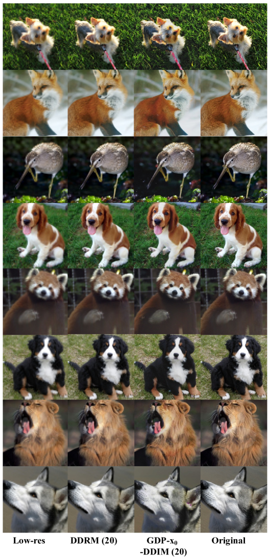
Figure 14: More samples from the 4 $\times$ super-resolution task of GDP-$\boldsymbol{x}_{0}$-DDIM (20) compare with DDRM (20) on 256 $\times$ 256 ImageNet 1K. The generated images by the DDRM (20) are still blurred, while our proposed GDP-$x_{0}$ with 20 steps of DDIM sampling can restore more details.

To accelerate the sampling strategy, GDP follows [58] to use DDIM, which skipping steps in the reverse process to speed up the DDPM generating process. We apply this method to the ImageNet dataset on the four tasks. We set the $T$=20 in the sampling process, while DDRM also utilizes the same time steps for a fair comparison. As shown in Table 9, our GDP-$x_{0}$-DDIM(20) outperforms DDRM(20) on consistency and FID across four tasks. Although DDRM(20) obtains better PSNR and SSIM than our GDP-$x_{0}$-DDIM(20), the qualitative results of DDRM(20) are still worse than our GDP-$x_{0}$-DDIM(20), which can be seen from Figs. 14 and 15. Previous work [73, 11, 13, 17] demonstrated that these conventional automated evaluation measures (PSNR and SSIM) do not correlate well with human perception when the input resolution is low, and the magnification is large. This is not surprising since these metrics tend to penalize any synthesized high-frequency detail that is not perfectly aligned with the target image.

Table 9: The performances of DDRM (20) and GDM-$\boldsymbol{x}_{0}$-DDIM(20) towards the four tasks on ImageNet 1k. The DDIM sample steps are all set to 20 to make a fair comparison.

Task	4$\times$ super resolution				Deblur				25% Impainting				Colorization
	PSNR	SSIM	Consistency	FID	PSNR	SSIM	Consistency	FID	PSNR	SSIM	Consistency	FID	PSNR	SSIM	Consistency	FID
DDRM(20) [32]	26.53	0.784	19.39	40.75	35.64	0.978	50.24	4.78	34.28	0.958	4.08	24.09	22.12	0.924	38.66	47.05
GDP-$x_{0}$-DDIM(20)	23.77	0.623	9.24	39.46	24.87	0.683	44.39	3.66	30.82	0.892	7.10	19.70	21.13	0.840	37.33	41.38

Table 10: The time comparison of GDP-$x_{0}$-DDIM(20) and GDP-$x_{0}$ on 4x super-resolution. These experiments are compared on Tesla A100.

		Guidance scale	Total steps	Guidance times per steps	Generation time per image
GDP-$x_{0}$	w.o. DDIM	2e3	1000	6	69.55
GDP-$x_{0}$-DDIM(20)	w. DDIM	22e5	20	20	1.74

Table 11: The quantitative comparison of performance on CelebA.

CelebA	4x SR				Deblur				25% Inpainting
	PSNR	SSIM	Consistency	FID	PSNR	SSIM	Consistency	FID	PSNR	SSIM	Consistency	FID
DDRM	29.50	0.863	6.82	87.71	36.51	0.98	35.91	14.30	31.99	0.918	0.47	69.46
GDP-$x_{t}$	29.19	0.847	14.11	94.98	27.35	0.81	34.87	9.97	36.19	0.963	1.94	22.53
GDP-$x_{0}$	30.26	0.868	5.33	46.64	28.66	0.83	32.66	4.50	37.70	0.972	0.51	11.62

Table 12: The quantitative comparison of results on LSUN bedroom.

LSUN Bedroom	4x SR		Deblur		25% Inpainting		Colorization
	Consistency	FID	Consistency	FID	Consistency	FID	Consistency	FID
DDRM	20.33	40.12	43.78	10.16	5.33	22.49	35.16	45.22
GDP-$x_{t}$	70.46	58.62	46.90	12.50	9.33	20.63	66.88	57.13
GDP-$x_{0}$	7.66	36.94	42.28	9.51	6.77	18.34	33.51	34.59

Table 13: The weight of reconstruction loss and quality enhancement loss.

	MSE loss	Exposure Control Loss	Color Constancy Loss	Illumination Smoothness Loss
Colorization	1	0	500	0
Low-light Enhancement	1	1/100	1/200	1
HDR recovery	1	1/100	1/200	1

Appendix H Image Guidance

A conditioner $p(\boldsymbol{y}\mid{\boldsymbol{x}})$ is exploited to improve a diffusion generator. Specifically, we can utilize a conditioner $p_{\phi}\left(\boldsymbol{y}\mid\boldsymbol{x}_{t},t\right)$ on input images, and then use gradients $\nabla_{\boldsymbol{x}_{t}}\log p_{\phi}\left(\boldsymbol{y}\mid\boldsymbol{x}_{t},t\right)$ to guide the diffusion sampling process towards a given the degraded images $\boldsymbol{y}$.

In this section, we will describe how to use such conditioners to improve the quality of sampled images. The notation is chosen as $p_{\phi}\left(\boldsymbol{y}\mid\boldsymbol{x}_{t},t\right)=p_{\phi}\left(\boldsymbol{y}\mid\boldsymbol{x}_{t}\right)$ and $\epsilon_{\theta}\left(\boldsymbol{x}_{t},t\right)=\epsilon_{\theta}\left(\boldsymbol{x}_{t}\right)$ for brevity. Note that they refer to separate functions for each time step $t$.

H.1 Conditional Reverse Process

Assume a diffusion model with an unconditional reverse noising process $p_{\theta}\left(\boldsymbol{x}_{t}\mid\boldsymbol{x}_{t+1}\right)$. In image restoration and enhancement, the corrupted inputs can be regarded as conditions. Therefore, we regard $\boldsymbol{y}$ as the input images, and $\boldsymbol{x}_{t}$ as the generated images in time step $t$. Then, the conditioner is formulated as follows:

$$p_{\phi}\left(\boldsymbol{y}\mid\boldsymbol{x}_{t}\right)=\frac{1}{K}exp\left(-\mathcal{L}\left(\boldsymbol{y},\mathcal{D}\left(\boldsymbol{x}_{t}\right)\right)\right),$$ (17)

where $\mathcal{D}$ represents the degradation function, $\mathcal{L}$ stands for Mean Square Error together with optional Quality Enhancement Loss, and $K$ is an arbitrary constant. In order to condition this on the input corrupted image $\boldsymbol{y}$, it is sufficient to sample each transition based on the following:

$$p_{\theta,\phi}\left(\boldsymbol{x}_{t}\mid\boldsymbol{x}_{t+1},\boldsymbol{y}\right)=Cp_{\theta}\left(\boldsymbol{x}_{t}\mid\boldsymbol{x}_{t+1}\right)p_{\phi}\left(\boldsymbol{y}\mid\boldsymbol{x}_{t}\right)$$ (18)

where $C$ denotes a normalizing constant. It is typically intractable to sample from this distribution exactly, but Sohl-Dickstein et al. [76] show that it can be approximated as a perturbed Gaussian distribution. Sampling accurately from this distribution is often tricky, but Sohl-Dickstein et al. [76] prove that it could be approximated as a perturbed Gaussian distribution. It is formulated that the diffusion model samples the previous time step $\boldsymbol{x}_{t}$ from time step $\boldsymbol{x}_{t+1}$ via a Gaussian distribution:

$$p_{\theta}\left(\boldsymbol{x}_{t}\mid\boldsymbol{x}_{t+1}\right)=\mathcal{N}(\mu,\Sigma)$$ (19)

$$\log p_{\theta}\left(\boldsymbol{x}_{t}\mid\boldsymbol{x}_{t+1}\right)=-\frac{1}{2}\left(\boldsymbol{x}_{t}-\mu\right)_{T}\Sigma^{-1}\left(\boldsymbol{x}_{t}-\mu\right)+Z$$ (20)

We can assume that $\log_{\phi}p\left(\boldsymbol{y}\mid\boldsymbol{x}_{t}\right)$ owns low curvature when compared with $\Sigma^{-1}$. This assumption is reasonable under the constraint that the infinite diffusion step, where $\|\Sigma\|\rightarrow 0$. Under the circumstances, $\log p_{\phi}\left(\boldsymbol{y}\mid\boldsymbol{x}_{t}\right)$ can be approximated via a Taylor expansion around $\boldsymbol{x}_{t}=\mu$ as:

$$\log p_{\phi}\left(\boldsymbol{y}\mid\boldsymbol{x}_{t}\right) \left.\approx\log p_{\phi}\left(\boldsymbol{y}\mid\boldsymbol{x}_{t}\right)\right|_{\boldsymbol{x}_{t}=\mu}$$ (21)

$$+\left.\left(\boldsymbol{x}_{t}-\mu\right)\nabla_{\boldsymbol{x}_{t}}\log p_{\phi}\left(\boldsymbol{y}\mid\boldsymbol{x}_{t}\right)\right|_{\boldsymbol{x}_{t}=\mu}$$

$$=\left(\boldsymbol{x}_{t}-\mu\right)g+Z_{1}$$

Here, $g=\nabla_{\boldsymbol{x}_{t}}\log p_{\phi}\left(\boldsymbol{y}\mid\boldsymbol{x}_{t}\right)\|_{\boldsymbol{x}_{t}=\mu}$, and $Z_{1}$ is a constant. We can replace the $g$ with Eq. 17 as follows:

$$\log p\left(\boldsymbol{y}\mid\boldsymbol{x}_{t}\right)=-\mathcal{L}\left(\boldsymbol{y},\mathcal{D}\left(\boldsymbol{x}_{t}\right)\right)-\log K$$ (22)

$$g=\nabla_{\boldsymbol{x}_{t}}\log p\left(\boldsymbol{y}\mid\boldsymbol{x}_{t}\right)=-\nabla_{\boldsymbol{x}_{t}}\mathcal{L}\left(\boldsymbol{y},\mathcal{D}\left(\boldsymbol{x}_{t}\right)\right)$$ (23)

This gives:

$$\log\left(p_{\theta}\left(\boldsymbol{x}_{t}\mid\boldsymbol{x}_{t+1}\right)p_{\phi}\left(\boldsymbol{y}\mid\boldsymbol{x}_{t}\right)\right)$$ (24)

$$\approx-\frac{1}{2}\left(\boldsymbol{x}_{t}-\mu\right)^{T}\Sigma^{-1}\left(\boldsymbol{x}_{t}-\mu\right)+\left(\boldsymbol{x}_{t}-\mu\right)g+Z_{2}$$

$$=-\frac{1}{2}\left(\boldsymbol{x}_{t}-\mu-\Sigma g\right)^{T}\Sigma^{-1}\left(\boldsymbol{x}_{t}-\mu-\Sigma g\right)+\frac{1}{2}g^{T}\Sigma g+Z_{2}$$

$$=-\frac{1}{2}\left(\boldsymbol{x}_{t}-\mu-\Sigma g\right)^{T}\Sigma^{-1}\left(\boldsymbol{x}_{t}-\mu-\Sigma g\right)+Z_{3}$$

$$=\log p(z)+Z_{4},z\sim\mathcal{N}(\mu+\Sigma g,\Sigma)$$

where the constant term $C_{4}$ could be safely ignored because it is equivalent to the normalizing coefficient $Z$ in Eq. 18. Thus, we find that the conditional transition operator can be approximated by a Gaussian similar to the unconditional transition operator, but with a mean shifted by $\Sigma g$. Moreover, an optional scaling factor $s$ is included for gradients, which will be described in more detail in Sec. H.3. However, it is experimentally found that this guidance way might not be effective enough, where our GDP-$x_{0}$ is systematically studied.

H.2 Conditional Diffusion Process

Here, we figure out that conditional sampling can be fulfilled with a transition operator proportional to $p_{\theta}\left(\boldsymbol{x}_{t}\mid\boldsymbol{x}_{t+1}\right)p_{\phi}\left(\boldsymbol{y}\mid\boldsymbol{x}_{t}\right)$, where $p_{\theta}\left(\boldsymbol{x}_{t}\mid\boldsymbol{x}_{t+1}\right)$ approximates $q\left(\boldsymbol{x}_{t}\mid\boldsymbol{x}_{t+1}\right)$ and $p_{\phi}\left(\boldsymbol{y}\mid\boldsymbol{x}_{t}\right)$ approximates the distribution of the input for a noised sample $\boldsymbol{x}_{t}$.

A conditional Markovian noising process $\hat{q}$ is similar to $q$. And $\hat{q}\left(\boldsymbol{y}\mid\boldsymbol{x}_{0}\right)$ is assumed as a known and readily available degraded images distribution for each sample.

$$\hat{q}\left(\boldsymbol{x}_{0}\right) :=q\left(\boldsymbol{x}_{0}\right)$$ (25)

$$\hat{q}\left(\boldsymbol{y}\mid\boldsymbol{x}_{0}\right) :=\text{Corrupted input image per sample}$$ (26)

$$\hat{q}\left(\boldsymbol{x}_{t+1}\mid\boldsymbol{x}_{t},\boldsymbol{y}\right) :=q\left(\boldsymbol{x}_{t+1}\mid\boldsymbol{x}_{t}\right)$$ (27)

$$\hat{q}\left(\boldsymbol{x}_{1:T}\mid\boldsymbol{x}_{0},\boldsymbol{y}\right) :=\prod_{t=1}^{T}\hat{q}\left(\boldsymbol{x}_{t}\mid\boldsymbol{x}_{t-1},\boldsymbol{y}\right)$$ (28)

Assuming that the noising process $\hat{q}$ is conditioned on $\boldsymbol{y}$, we can reveal that $\hat{q}$ behaves exactly like $q$ when not conditioned on $\boldsymbol{y}$. According to this idea, we first derive the unconditional noising operator $\hat{q}\left(\boldsymbol{x}_{t+1}\mid\boldsymbol{x}_{t}\right)$ :

$$\hat{q}\left(\boldsymbol{x}_{t+1}\mid\boldsymbol{x}_{t}\right) =\int_{\boldsymbol{y}}\hat{q}\left(\boldsymbol{x}_{t+1},\boldsymbol{y}\mid\boldsymbol{x}_{t}\right)d\boldsymbol{y}$$ (29)

$$=\int_{\boldsymbol{y}}\hat{q}\left(\boldsymbol{x}_{t+1}\mid\boldsymbol{x}_{t},\boldsymbol{y}\right)\hat{q}\left(\boldsymbol{y}\mid\boldsymbol{x}_{t}\right)d\boldsymbol{y}$$ (30)

$$=\int_{\boldsymbol{y}}q\left(\boldsymbol{x}_{t+1}\mid\boldsymbol{x}_{t}\right)\hat{q}\left(\boldsymbol{y}\mid\boldsymbol{x}_{t}\right)d\boldsymbol{y}$$ (31)

$$=q\left(\boldsymbol{x}_{t+1}\mid\boldsymbol{x}_{t}\right)\int_{\boldsymbol{y}}\hat{q}\left(\boldsymbol{y}\mid\boldsymbol{x}_{t}\right)d\boldsymbol{y}$$ (32)

$$=q\left(\boldsymbol{x}_{t+1}\mid\boldsymbol{x}_{t}\right)$$ (33)

$$=\hat{q}\left(\boldsymbol{x}_{t+1}\mid\boldsymbol{x}_{t},\boldsymbol{y}\right)$$ (34)

Similarly, the joint distribution $\hat{q}\left(\boldsymbol{x}_{1:T}\mid\boldsymbol{x}_{0}\right)$ can be written as:

$$\hat{q}\left(\boldsymbol{x}_{1:T}\mid\boldsymbol{x}_{0}\right) =\int_{\boldsymbol{y}}\hat{q}\left(\boldsymbol{x}_{1:T},\boldsymbol{y}\mid\boldsymbol{x}_{0}\right)d\boldsymbol{y}$$ (35)

$$=\int_{\boldsymbol{y}}\hat{q}\left(\boldsymbol{y}\mid\boldsymbol{x}_{0}\right)\hat{q}\left(\boldsymbol{x}_{1:T}\mid\boldsymbol{x}_{0},\boldsymbol{y}\right)d\boldsymbol{y}$$ (36)

$$=\int_{\boldsymbol{y}}\hat{q}\left(\boldsymbol{y}\mid\boldsymbol{x}_{0}\right)\prod_{t=1}^{T}\hat{q}\left(\boldsymbol{x}_{t}\mid\boldsymbol{x}_{t-1},\boldsymbol{y}\right)d\boldsymbol{y}$$ (37)

$$=\int_{\boldsymbol{y}}\hat{q}\left(\boldsymbol{y}\mid\boldsymbol{x}_{0}\right)\prod_{t=1}^{T}q\left(\boldsymbol{x}_{t}\mid\boldsymbol{x}_{t-1}\right)d\boldsymbol{y}$$ (38)

$$=\prod_{t=1}^{T}q\left(\boldsymbol{x}_{t}\mid\boldsymbol{x}_{t-1}\right)\int_{\boldsymbol{y}}\hat{q}\left(\boldsymbol{y}\mid\boldsymbol{x}_{0}\right)d\boldsymbol{y}$$ (39)

$$=\prod_{t=1}^{T}q\left(\boldsymbol{x}_{t}\mid\boldsymbol{x}_{t-1}\right)$$ (40)

$$=q\left(\boldsymbol{x}_{1:T}\mid\boldsymbol{x}_{0}\right)$$ (41)

$\hat{q}\left(\boldsymbol{x}_{t}\right)$ can be derived by using Eq. 41 as follows:

$$\hat{q}\left(\boldsymbol{x}_{t}\right) =\int_{\boldsymbol{x}_{0:t-1}}\hat{q}\left(\boldsymbol{x}_{0},\ldots,\boldsymbol{x}_{t}\right)d\boldsymbol{x}_{0:t-1}$$ (42)

$$=\int_{\boldsymbol{x}_{0:t-1}}\hat{q}\left(\boldsymbol{x}_{0}\right)\hat{q}\left(\boldsymbol{x}_{1},\ldots,\boldsymbol{x}_{t}\mid\boldsymbol{x}_{0}\right)d\boldsymbol{x}_{0:t-1}$$ (43)

$$=\int_{\boldsymbol{x}_{0:t-1}}q\left(\boldsymbol{x}_{0}\right)q\left(\boldsymbol{x}_{1},\ldots,\boldsymbol{x}_{t}\mid\boldsymbol{x}_{0}\right)d\boldsymbol{x}_{0:t-1}$$ (44)

$$=\int_{\boldsymbol{x}_{0:t-1}}q\left(\boldsymbol{x}_{0},\ldots,\boldsymbol{x}_{t}\right)d\boldsymbol{x}_{0:t-1}$$ (45)

$$=q\left(\boldsymbol{x}_{t}\right)$$ (46)

It is proved by Bayes rule that the unconditional reverse process $\hat{q}\left(\boldsymbol{x}_{t}\mid\boldsymbol{x}_{t+1}\right)=q\left(\boldsymbol{x}_{t}\mid\boldsymbol{x}_{t+1}\right)$ when using the identities $\hat{q}\left(\boldsymbol{x}_{t}\right)=q\left(\boldsymbol{x}_{t}\right)$ and $\hat{q}\left(\boldsymbol{x}_{t+1}\mid\boldsymbol{x}_{t}\right)=q\left(\boldsymbol{x}_{t+1}\mid\boldsymbol{x}_{t}\right)$.

Note that $\hat{q}$ is able to produce an input function $\hat{q}\left(\boldsymbol{y}\mid\boldsymbol{x}_{t}\right)$. It is shown that this distribution of the input does not depend on $\boldsymbol{x}_{t+1}$ (the noisy version of $\boldsymbol{x}_{t}$), we will discuss this fact later by exploiting:

$$\hat{q}\left(\boldsymbol{y}\mid\boldsymbol{x}_{t},\boldsymbol{x}_{t+1}\right) =\hat{q}\left(\boldsymbol{x}_{t+1}\mid\boldsymbol{x}_{t},\boldsymbol{y}\right)\frac{\hat{q}\left(\boldsymbol{y}\mid\boldsymbol{x}_{t}\right)}{\hat{q}\left(\boldsymbol{x}_{t+1}\mid\boldsymbol{x}_{t}\right)}$$ (47)

$$=\hat{q}\left(\boldsymbol{x}_{t+1}\mid\boldsymbol{x}_{t}\right)\frac{\hat{q}\left(\boldsymbol{y}\mid\boldsymbol{x}_{t}\right)}{\hat{q}\left(\boldsymbol{x}_{t+1}\mid\boldsymbol{x}_{t}\right)}$$ (48)

$$=\hat{q}\left(\boldsymbol{y}\mid\boldsymbol{x}_{t}\right)$$ (49)

In this way, the conditional reverse process can be derived as:

$$\hat{q}\left(\boldsymbol{x}_{t}\mid\boldsymbol{x}_{t+1},\boldsymbol{y}\right) =\frac{\hat{q}\left(\boldsymbol{x}_{t},\boldsymbol{x}_{t+1},\boldsymbol{y}\right)}{\hat{q}\left(\boldsymbol{x}_{t+1},\boldsymbol{y}\right)}$$ (50)

$$=\frac{\hat{q}\left(\boldsymbol{x}_{t},\boldsymbol{x}_{t+1},\boldsymbol{y}\right)}{\hat{q}\left(\boldsymbol{y}\mid\boldsymbol{x}_{t+1}\right)\hat{q}\left(\boldsymbol{x}_{t+1}\right)}$$ (51)

$$=\frac{\hat{q}\left(\boldsymbol{x}_{t}\mid\boldsymbol{x}_{t+1}\right)\hat{q}\left(\boldsymbol{y}\mid\boldsymbol{x}_{t},\boldsymbol{x}_{t+1}\right)\hat{q}\left(\boldsymbol{x}_{t+1}\right)}{\hat{q}\left(\boldsymbol{y}\mid\boldsymbol{x}_{t+1}\right)\hat{q}\left(\boldsymbol{x}_{t+1}\right)}$$ (52)

$$=\frac{\hat{q}\left(\boldsymbol{x}_{t}\mid\boldsymbol{x}_{t+1}\right)\hat{q}\left(\boldsymbol{y}\mid\boldsymbol{x}_{t},\boldsymbol{x}_{t+1}\right)}{\hat{q}\left(\boldsymbol{y}\mid\boldsymbol{x}_{t+1}\right)}$$ (53)

$$=\frac{\hat{q}\left(\boldsymbol{x}_{t}\mid\boldsymbol{x}_{t+1}\right)\hat{q}\left(\boldsymbol{y}\mid\boldsymbol{x}_{t}\right)}{\hat{q}\left(\boldsymbol{y}\mid\boldsymbol{x}_{t+1}\right)}$$ (54)

$$=\frac{q\left(\boldsymbol{x}_{t}\mid\boldsymbol{x}_{t+1}\right)\hat{q}\left(\boldsymbol{y}\mid\boldsymbol{x}_{t}\right)}{\hat{q}\left(\boldsymbol{y}\mid\boldsymbol{x}_{t+1}\right)}$$ (55)

where the $\hat{q}\left(\boldsymbol{y}\mid\boldsymbol{x}_{t+1}\right)$ can be treated as a constant because it does not depend on $\boldsymbol{x}_{t+1}$. Therefore, we want to sample from the distribution $Cq\left(\boldsymbol{x}_{t}\mid\boldsymbol{x}_{t+1}\right)\hat{q}\left(\boldsymbol{y}\mid\boldsymbol{x}_{t}\right)$ where $C$ denotes the normalization constant. We already have a neural network approximation of $q\left(\boldsymbol{x}_{t}\mid\boldsymbol{x}_{t+1}\right)$ called $p_{\theta}\left(\boldsymbol{x}_{t}\mid\boldsymbol{x}_{t+1}\right)$, so the rest is $\hat{q}\left(\boldsymbol{y}\mid\boldsymbol{x}_{t}\right)$ that can be obtained by computing a conditioner $p_{\phi}\left(\boldsymbol{y}\mid\boldsymbol{x}_{t}\right)$ on noised images $\boldsymbol{x}_{t}$ derived by sampling from $q\left(\boldsymbol{x}_{t}\right)$.

H.3 Scaling Conditioner Gradients

The conditioner is incorporated into the sampling process of the diffusion model using Eq. 24. To unveil the effect of scaling conditioner gradients, note that $s\cdot\nabla_{\boldsymbol{x}}\log p(\boldsymbol{y}\mid\boldsymbol{x})=\nabla_{\boldsymbol{x}}\log\frac{1}{K}p(\boldsymbol{y}\mid\boldsymbol{x})^{s}$, where $K$ is an arbitrary constant. Thus, the conditioning process is still theoretically based on the re-normalized distribution of the input proportional to $p(\boldsymbol{y}\mid\boldsymbol{x})^{s}$. If $s>1$, this distribution becomes sharper than $p(\boldsymbol{y}\mid\boldsymbol{x})$ because larger values are exponentially magnified. Therefore, using a larger gradient scale to focus more on the modes of the conditioner may be beneficial in producing higher fidelity (but less diverse) samples. In this paper, due to the observation that $\Sigma$ might exert a negative influence on the quality of images. Therefore, with the absence of the $\Sigma$, the guidance scale can be a variable scale $\hat{s}$, where $s=\Sigma\hat{s}$. Thanks to this variable scale $\hat{s}$, the quality of images can be promoted

Appendix I Additional Results on Linear inverse problems

We provide additional figures below showing GDP’s versatility across different datasets and linear inverse problems (Figures 16, 17, 18, 19), and 21). We present more uncurated samples from the ImageNet experiments in Figures 20, 22, 23, 24, 25, and 26. Moreover, our GDP is also able to recover the corrupted images that undergo multi-linear degradations, as shown in Fig. 27

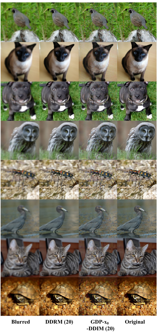
Figure 15: More samples from the deblurring task of GDP-$\boldsymbol{x}_{0}$-DDIM (20) compare with DDRM (20) on 256 $\times$ 256 ImageNet 1K. Our GDP-$x_{0}$-DDIM (20) can recover more details than DDRM (20) under the same DDIM steps.

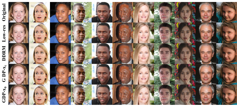
Figure 16: 4 $\times$ super-resolution results of DDRM, GDP-$\boldsymbol{x}_{t}$, and GDP-$\boldsymbol{x}_{0}$ on CelebA face images. Compared with GDP-$x_{t}$ and DDRM, GDP-$x_{0}$ can restore more realistic faces, such as the wrinkles on the faces, systematically demonstrating the superiority of the guidance on $x_{0}$ protocol.

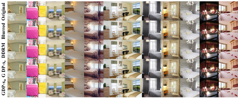
Figure 17: Deblurring results of DDRM, GDP-$\boldsymbol{x}_{t}$, and GDP-$\boldsymbol{x}_{0}$ on LSUN bedroom images.

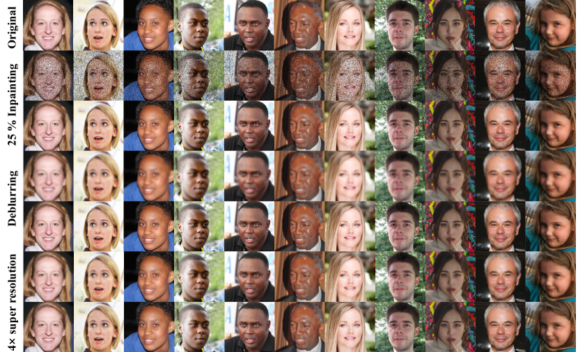
Figure 18: Pairs of degraded and recovered 256 $\times$ 256 CelebA face images with a GDP-$\boldsymbol{x}_{0}$. Three tasks including $25\%$ inpainting, deblurring and 4 $\times$ super-resolution are vividly depicted.

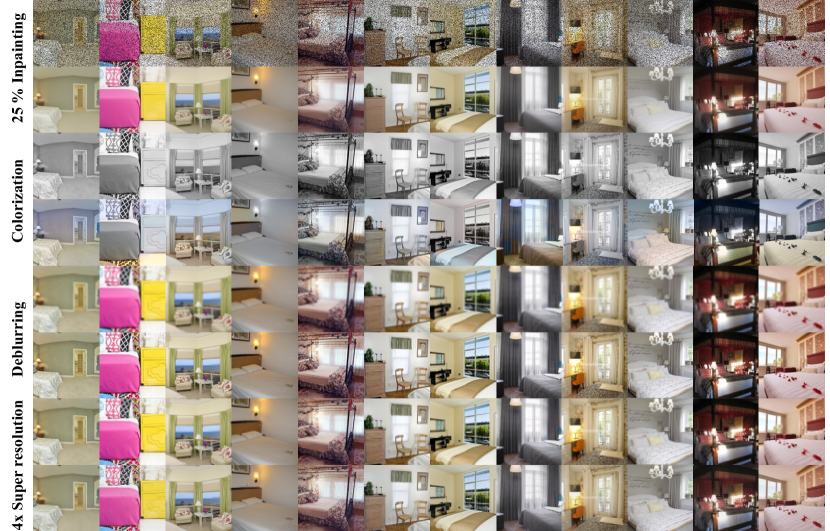
Figure 19: Pairs of degraded and recovered 256 $\times$ 256 LSUN bedroom images with a GDP-$\boldsymbol{x}_{0}$. We show more samples under the $25\%$ inpainting, colorization, deblurring and 4 $\times$ super-resolution.

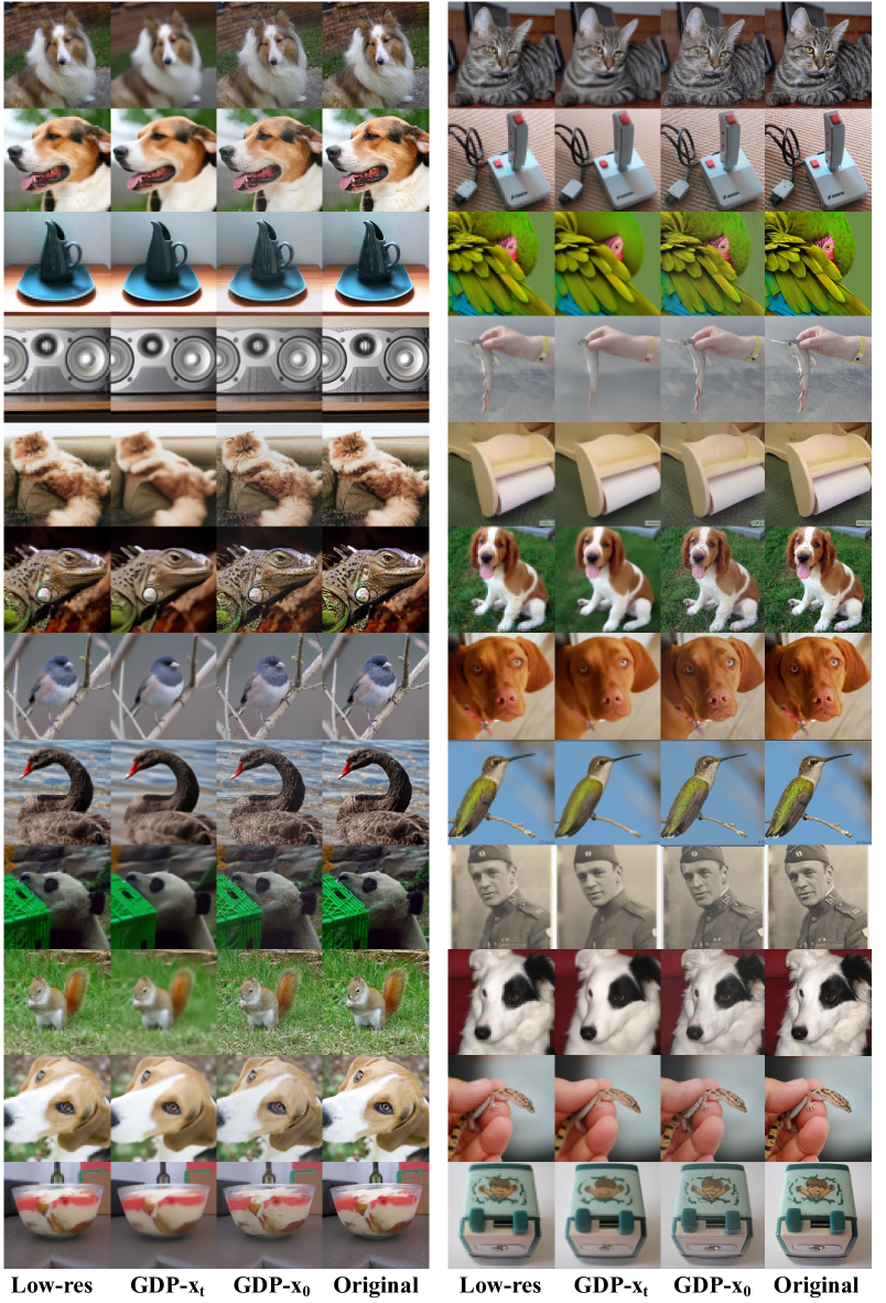
Figure 20: Uncurated samples from the 4 $\times$ super-resolution task on 256 $\times$ 256 ImageNet 1K.

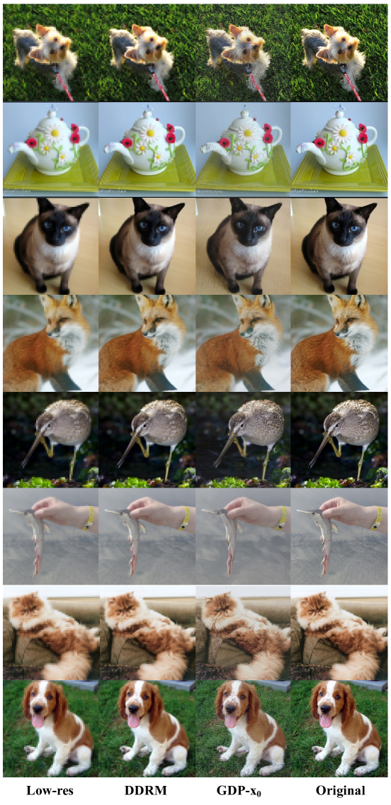
Figure 21: More samples from the 4 $\times$ super-resolution task compare with DDRM on 256 $\times$ 256 ImageNet 1K. As we mentioned above, DDRM adds guidance on the $x_{t}$, leading to the less satisfactory results than our GDP-$x_{0}$.

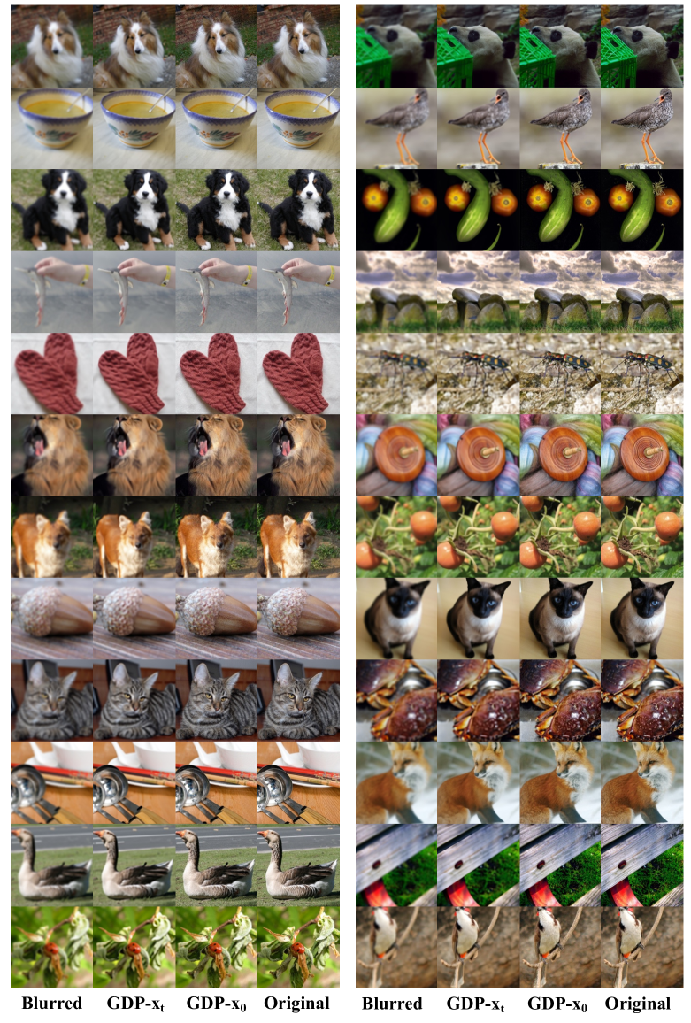
Figure 22: Uncurated samples from the deblurring task on 256 $\times$ 256 ImageNet 1K.

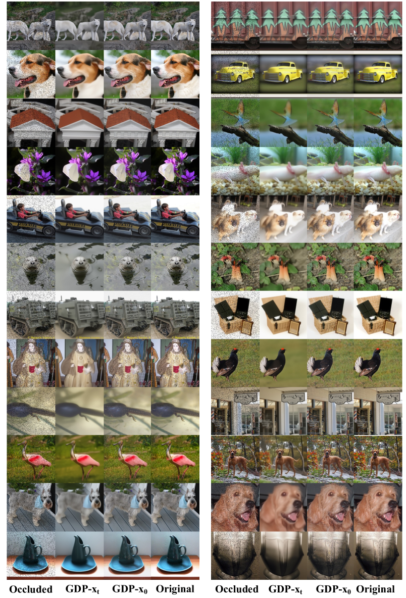
Figure 23: Uncurated samples from the $10\%$ inpainting task on 256 $\times$ 256 ImageNet 1K.

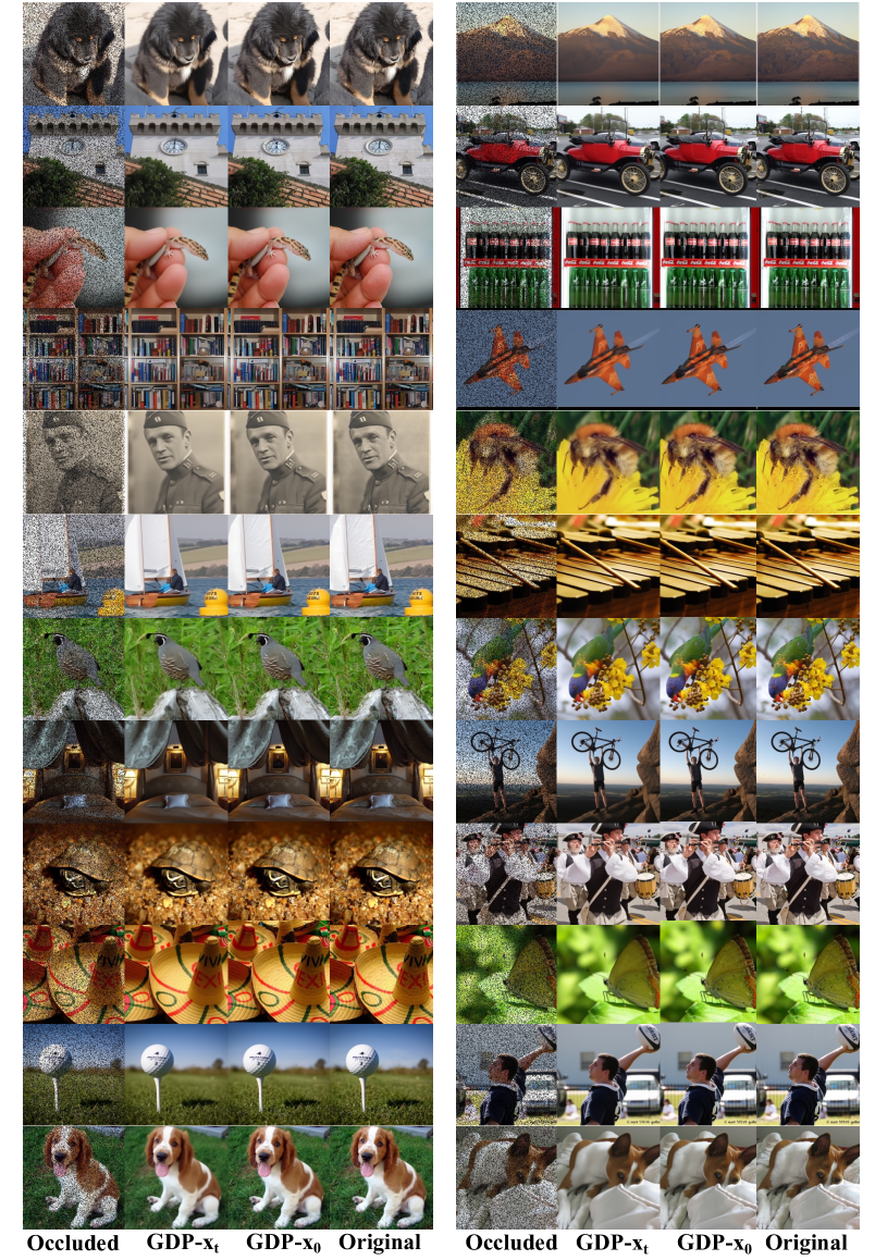
Figure 24: Uncurated samples from the $25\%$ inpainting task on 256 $\times$ 256 ImageNet 1K.

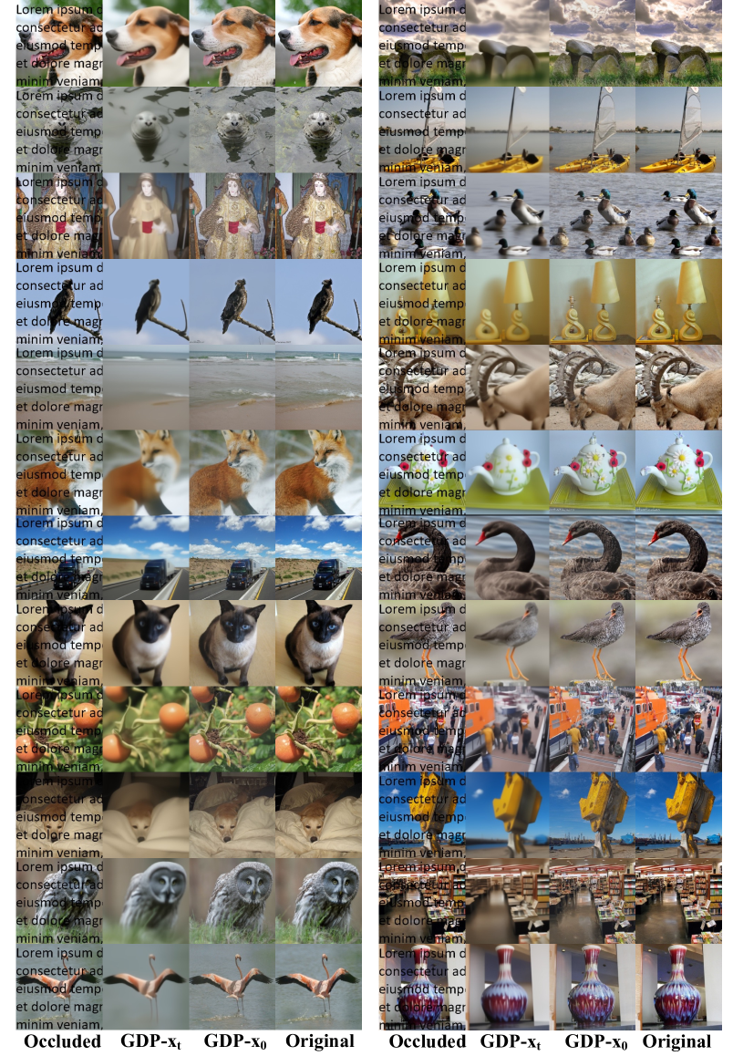
Figure 25: Uncurated samples from the inpainting task on 256 $\times$ 256 ImageNet 1K.

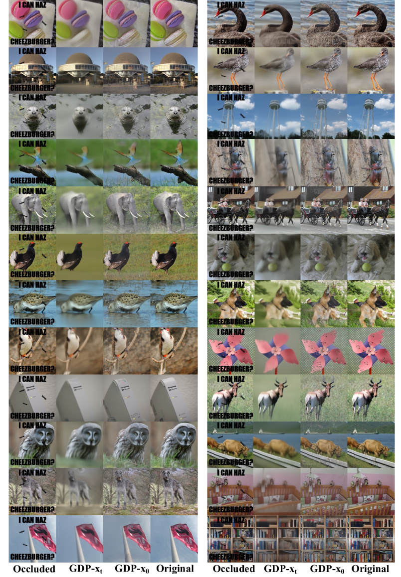
Figure 26: Uncurated samples from the inpainting task on 256 $\times$ 256 ImageNet 1K.

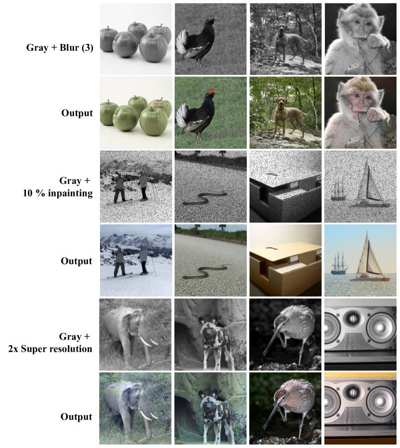
Figure 27: Samples from the multi-degradation tasks on 256 $\times$ 256 ImageNet 1K. It is shown that GDP can recover the corrupted images undergoing multiple degradations, such as gray + blur, gray + inpainting, and gray + down-sampling. It is noted that multi-linear degradation should be only one degradation model that will damage the contents of the images. In other words, the restoration will be more difficult if two content-damaged degradations occur at the same time, such as down-sampling + mask.

Appendix J Additional Results on Low-light Enhancement

In addition to the linear inverse problems, we further show more samples on the blind and non-linear task of low-light enhancement. As shown in 28, 31, and 33, our GDP performs well under the three datasets, including LOL, VE-LOL-L, and LoLi-phone, indicating the effectiveness of GDP under the different distributions of the images. Moreover, we also compare the GDP with other methods on the three datasets. As seen in 30, and 32, GDP-$x_{0}$ is able to generate more satisfactory images than other supervised learning, unsupervised learning, self-supervised, and zero-shot learning methods. Note that GDP-$x_{t}$ tends to yield images lighter than the ones generated by GDP-$x_{0}$. Furthermore, GDP can adjust the brightness of generated images by the Exposure Control Loss. As shown in 29, users can change the gray level $E$ in the RGB color space to obtain the target images with specific brightness.

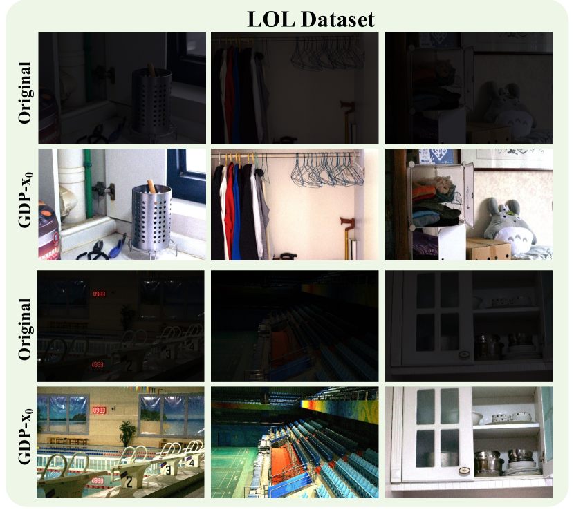
Figure 28: Results of low-light image enhancement on LOL dataset.

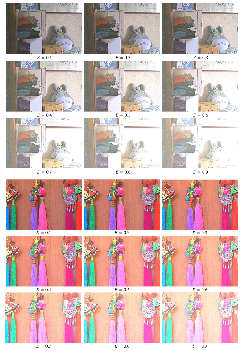
Figure 29: Results of light control on LOL dataset. We can adjust the brightness of the generated images with the help of Exposure Control Loss. Users can adjust the gray level $E$ in the RGB color space to obtain the images according to their needs.

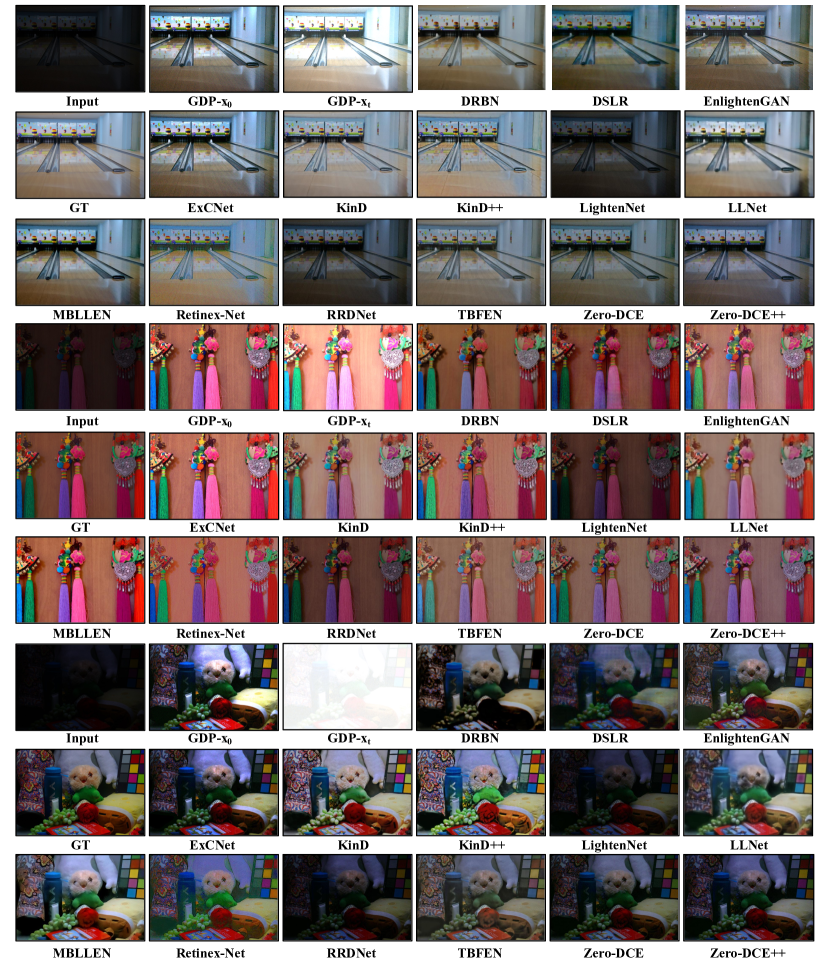
Figure 30: The comparison of our GDP and other methods on the LOL datasets towards low-light enhancement.

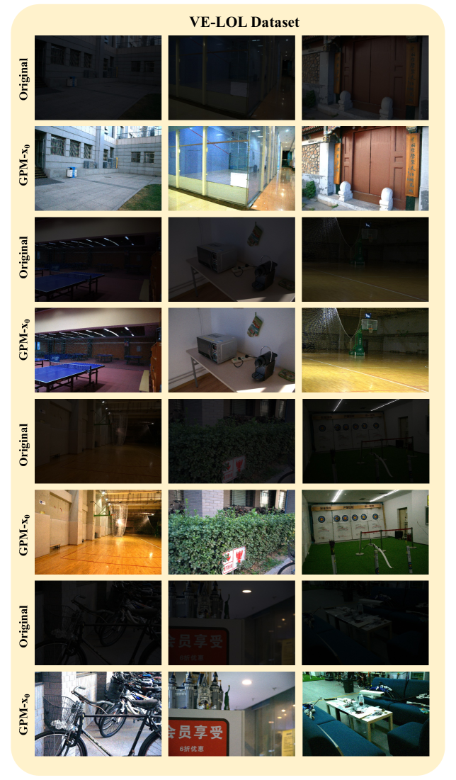
Figure 31: Results of low-light image enhancement on VE-LOL-L dataset.

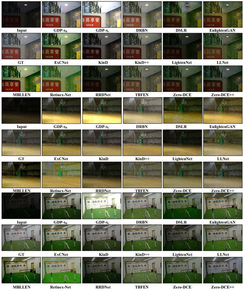
Figure 32: The comparison of our GDP and other methods on the VE-LOL-L datasets towards low-light enhancement.

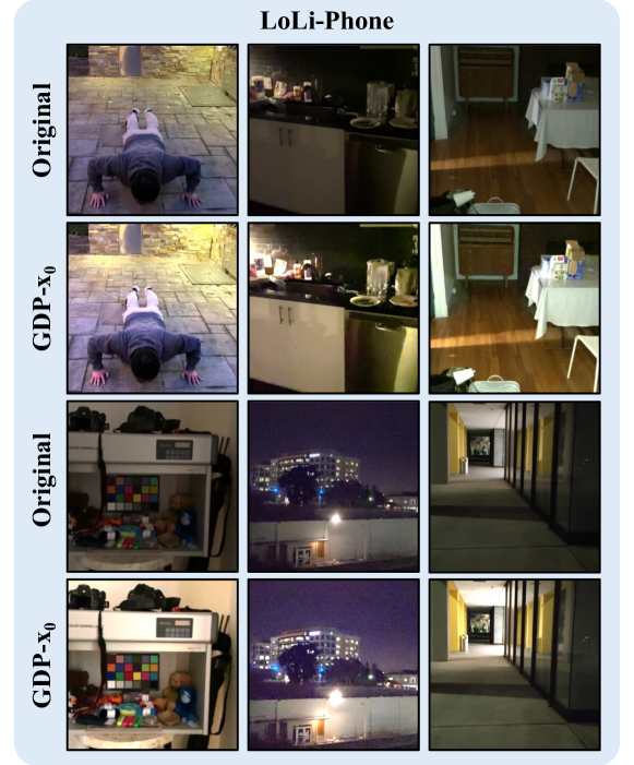
Figure 33: Results of low-light image enhancement on LoLi-Phone dataset.

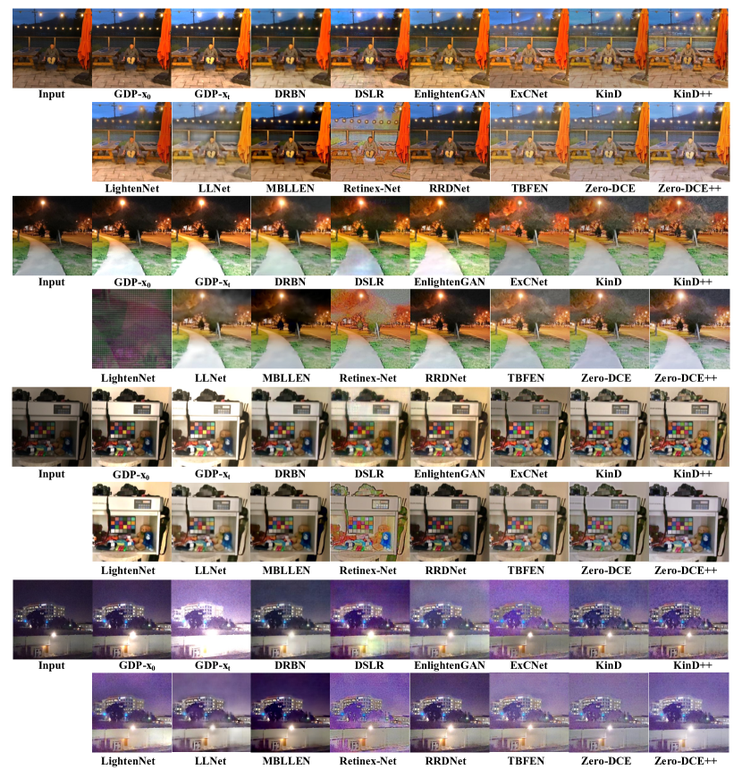
Figure 34: The comparison of our GDP and other methods on the LoLi-phone datasets towards low-light enhancement.

Appendix K Additional Results on HDR Recovery

As shown in 35, our HDR-GDP-$x_{0}$ is capable of adjusting the over-exposed and under-exposed areas of the picture in various scenes. It is noted that since the model used by GDP is pre-trained on ImageNet, the tone of the generated picture will be slightly different from ground truth images. Moreover, we also show more samples compared with the state-of-the-art methods, including AHDRNet [91], HDR-GAN [59], DeepHDR [90] and deep-high-dynamic-range [30]. As seen in Fig. 36, our HDR-GDP-$x_{0}$ can recover more realistic images with more details.

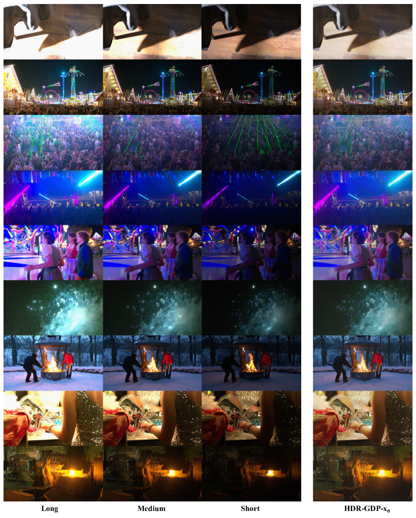
Figure 35: Results of HDR image recovery on NTIRE2021 dataset.

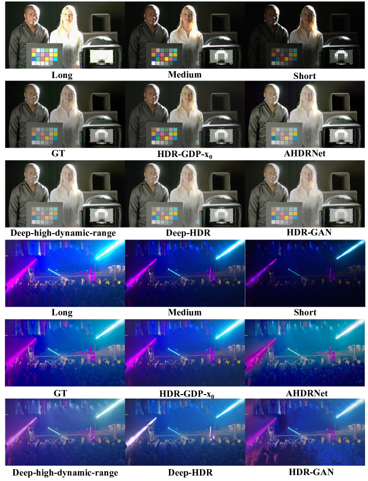
Figure 36: The comparison of HDR image recovery on NTIRE2021 dataset.

Appendix L Additional Results on Ablation Study

The visualization comparisons of the ablation study on the trainable degradation and the patch-based tactic are shown in Figs. 37 and 38. It is shown that Model A fails to generate high-quality images due to the interpolation operation, while Model B generates images with more artifacts because of the naive restoration. Model C predicts the outputs in an uncontrollable way thanks to the randomly initiated and fixed parameters.

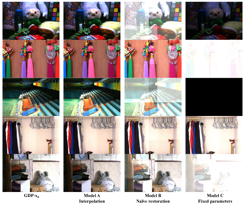
Figure 37: Qualitative comparison of ablation study on LOL dataset. Model A recovers the images in $256\times N$ or $256\times N$ sizes and is interpolated by the nearest neighbor to the original size. Model B is devised to naively restore the images from patches and patches where the parameters are not related. Model C is designed with fixed parameters for all patches in the images.

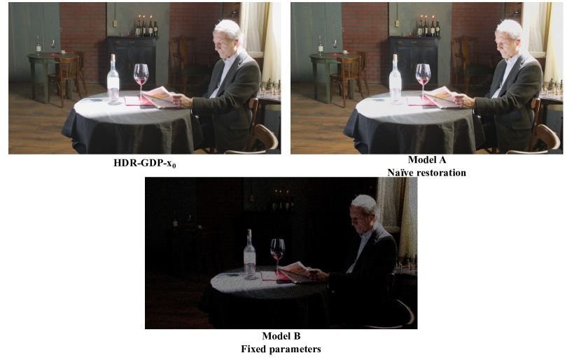
Figure 38: Qualitative comparison of ablation study on NTIRE2021 dataset.

References

- [1] Muhammad Asim, Fahad Shamshad, and Ali Ahmed. Blind image deconvolution using deep generative priors. IEEE Transactions on Computational Imaging, 6:1493–1506, 2020.
- [2] Jacob Austin, Daniel D Johnson, Jonathan Ho, Daniel Tarlow, and Rianne van den Berg. Structured denoising diffusion models in discrete state-spaces. Advances in Neural Information Processing Systems, 34:17981–17993, 2021.
- [3] Omri Avrahami, Dani Lischinski, and Ohad Fried. Blended diffusion for text-driven editing of natural images. In Proceedings of the IEEE/CVF Conference on Computer Vision and Pattern Recognition, pages 18208–18218, 2022.
- [4] Georgios Batzolis, Jan Stanczuk, Carola-Bibiane Schönlieb, and Christian Etmann. Conditional image generation with score-based diffusion models. arXiv preprint arXiv:2111.13606, 2021.
- [5] Isabelle Begin and FR Ferrie. Blind super-resolution using a learning-based approach. In Proceedings of the 17th International Conference on Pattern Recognition, 2004. ICPR 2004., volume 2, pages 85–89. IEEE, 2004.
- [6] Gershon Buchsbaum. A spatial processor model for object colour perception. Journal of the Franklin institute, 310(1):1–26, 1980.
- [7] Ruojin Cai, Guandao Yang, Hadar Averbuch-Elor, Zekun Hao, Serge Belongie, Noah Snavely, and Bharath Hariharan. Learning gradient fields for shape generation. In European Conference on Computer Vision, pages 364–381. Springer, 2020.
- [8] Jingwen Chen, Jiawei Chen, Hongyang Chao, and Ming Yang. Image blind denoising with generative adversarial network based noise modeling. In Proceedings of the IEEE conference on computer vision and pattern recognition, pages 3155–3164, 2018.
- [9] Nanxin Chen, Yu Zhang, Heiga Zen, Ron J Weiss, Mohammad Norouzi, and William Chan. Wavegrad: Estimating gradients for waveform generation. arXiv preprint arXiv:2009.00713, 2020.
- [10] Xiangyu Chen, Yihao Liu, Zhengwen Zhang, Yu Qiao, and Chao Dong. Hdrunet: Single image hdr reconstruction with denoising and dequantization. In Proceedings of the IEEE/CVF Conference on Computer Vision and Pattern Recognition, pages 354–363, 2021.
- [11] Yu Chen, Ying Tai, Xiaoming Liu, Chunhua Shen, and Jian Yang. Fsrnet: End-to-end learning face super-resolution with facial priors. In Proceedings of the IEEE Conference on Computer Vision and Pattern Recognition, pages 2492–2501, 2018.
- [12] Jooyoung Choi, Jungbeom Lee, Chaehun Shin, Sungwon Kim, Hyunwoo Kim, and Sungroh Yoon. Perception prioritized training of diffusion models. In Proceedings of the IEEE/CVF Conference on Computer Vision and Pattern Recognition, pages 11472–11481, 2022.
- [13] Ryan Dahl, Mohammad Norouzi, and Jonathon Shlens. Pixel recursive super resolution. In Proceedings of the IEEE international conference on computer vision, pages 5439–5448, 2017.
- [14] Jia Deng, Wei Dong, Richard Socher, Li-Jia Li, Kai Li, and Li Fei-Fei. Imagenet: A large-scale hierarchical image database. In 2009 IEEE conference on computer vision and pattern recognition, pages 248–255. Ieee, 2009.
- [15] Prafulla Dhariwal and Alexander Nichol. Diffusion models beat gans on image synthesis. Advances in Neural Information Processing Systems, 34:8780–8794, 2021.
- [16] Chao Dong, Chen Change Loy, Kaiming He, and Xiaoou Tang. Image super-resolution using deep convolutional networks. IEEE transactions on pattern analysis and machine intelligence, 38(2):295–307, 2015.
- [17] Alexey Dosovitskiy and Thomas Brox. Generating images with perceptual similarity metrics based on deep networks. Advances in neural information processing systems, 29, 2016.
- [18] Wenchao Du, Hu Chen, and Hongyu Yang. Learning invariant representation for unsupervised image restoration. In Proceedings of the ieee/cvf conference on computer vision and pattern recognition, pages 14483–14492, 2020.
- [19] Majed El Helou and Sabine Süsstrunk. Bigprior: Toward decoupling learned prior hallucination and data fidelity in image restoration. IEEE Transactions on Image Processing, 31:1628–1640, 2022.
- [20] Ian Goodfellow, Jean Pouget-Abadie, Mehdi Mirza, Bing Xu, David Warde-Farley, Sherjil Ozair, Aaron Courville, and Yoshua Bengio. Generative adversarial networks. Communications of the ACM, 63(11):139–144, 2020.
- [21] Jinjin Gu, Yujun Shen, and Bolei Zhou. Image processing using multi-code gan prior. In Proceedings of the IEEE/CVF conference on computer vision and pattern recognition, pages 3012–3021, 2020.
- [22] Shuyang Gu, Dong Chen, Jianmin Bao, Fang Wen, Bo Zhang, Dongdong Chen, Lu Yuan, and Baining Guo. Vector quantized diffusion model for text-to-image synthesis. In Proceedings of the IEEE/CVF Conference on Computer Vision and Pattern Recognition, pages 10696–10706, 2022.
- [23] Chunle Guo, Chongyi Li, Jichang Guo, Chen Change Loy, Junhui Hou, Sam Kwong, and Runmin Cong. Zero-reference deep curve estimation for low-light image enhancement. In Proceedings of the IEEE/CVF Conference on Computer Vision and Pattern Recognition, pages 1780–1789, 2020.
- [24] Muhammad Haris, Gregory Shakhnarovich, and Norimichi Ukita. Deep back-projection networks for super-resolution. In Proceedings of the IEEE conference on computer vision and pattern recognition, pages 1664–1673, 2018.
- [25] Yu He, Kim-Hui Yap, Li Chen, and Lap-Pui Chau. A soft map framework for blind super-resolution image reconstruction. Image and Vision Computing, 27(4):364–373, 2009.
- [26] Martin Heusel, Hubert Ramsauer, Thomas Unterthiner, Bernhard Nessler, and Sepp Hochreiter. Gans trained by a two time-scale update rule converge to a local nash equilibrium. Advances in neural information processing systems, 30, 2017.
- [27] Jonathan Ho, Ajay Jain, and Pieter Abbeel. Denoising diffusion probabilistic models. Advances in Neural Information Processing Systems, 33:6840–6851, 2020.
- [28] Jonathan Ho, Chitwan Saharia, William Chan, David J Fleet, Mohammad Norouzi, and Tim Salimans. Cascaded diffusion models for high fidelity image generation. J. Mach. Learn. Res., 23:47–1, 2022.
- [29] Yifan Jiang, Xinyu Gong, Ding Liu, Yu Cheng, Chen Fang, Xiaohui Shen, Jianchao Yang, Pan Zhou, and Zhangyang Wang. Enlightengan: Deep light enhancement without paired supervision. IEEE Transactions on Image Processing, 30:2340–2349, 2021.
- [30] Nima Khademi Kalantari, Ravi Ramamoorthi, et al. Deep high dynamic range imaging of dynamic scenes. ACM Trans. Graph., 36(4):144–1, 2017.
- [31] Tero Karras, Timo Aila, Samuli Laine, and Jaakko Lehtinen. Progressive growing of gans for improved quality, stability, and variation. arXiv preprint arXiv:1710.10196, 2017.
- [32] Bahjat Kawar, Michael Elad, Stefano Ermon, and Jiaming Song. Denoising diffusion restoration models. arXiv preprint arXiv:2201.11793, 2022.
- [33] Bahjat Kawar, Gregory Vaksman, and Michael Elad. Snips: Solving noisy inverse problems stochastically. Advances in Neural Information Processing Systems, 34:21757–21769, 2021.
- [34] Rihuan Ke and Carola-Bibiane Schönlieb. Unsupervised image restoration using partially linear denoisers. IEEE Transactions on Pattern Analysis and Machine Intelligence, 44(9):5796–5812, 2021.
- [35] Jiwon Kim, Jung Kwon Lee, and Kyoung Mu Lee. Deeply-recursive convolutional network for image super-resolution. In Proceedings of the IEEE conference on computer vision and pattern recognition, pages 1637–1645, 2016.
- [36] Diederik Kingma, Tim Salimans, Ben Poole, and Jonathan Ho. Variational diffusion models. Advances in neural information processing systems, 34:21696–21707, 2021.
- [37] Orest Kupyn, Tetiana Martyniuk, Junru Wu, and Zhangyang Wang. Deblurgan-v2: Deblurring (orders-of-magnitude) faster and better. In Proceedings of the IEEE/CVF International Conference on Computer Vision, pages 8878–8887, 2019.
- [38] Gustav Larsson, Michael Maire, and Gregory Shakhnarovich. Learning representations for automatic colorization. In European conference on computer vision, pages 577–593. Springer, 2016.
- [39] Christian Ledig, Lucas Theis, Ferenc Huszár, Jose Caballero, Andrew Cunningham, Alejandro Acosta, Andrew Aitken, Alykhan Tejani, Johannes Totz, Zehan Wang, et al. Photo-realistic single image super-resolution using a generative adversarial network. In Proceedings of the IEEE conference on computer vision and pattern recognition, pages 4681–4690, 2017.
- [40] Cheng-Han Lee, Ziwei Liu, Lingyun Wu, and Ping Luo. Maskgan: Towards diverse and interactive facial image manipulation. In Proceedings of the IEEE/CVF Conference on Computer Vision and Pattern Recognition, pages 5549–5558, 2020.
- [41] Chongyi Li, Chunle Guo, Ling-Hao Han, Jun Jiang, Ming-Ming Cheng, Jinwei Gu, and Chen Change Loy. Low-light image and video enhancement using deep learning: A survey. IEEE Transactions on Pattern Analysis & Machine Intelligence, 44(01):1–1, 2021.
- [42] Chongyi Li, Chunle Guo, and Chen Change Loy. Learning to enhance low-light image via zero-reference deep curve estimation. arXiv preprint arXiv:2103.00860, 2021.
- [43] Chongyi Li, Jichang Guo, Fatih Porikli, and Yanwei Pang. Lightennet: A convolutional neural network for weakly illuminated image enhancement. Pattern recognition letters, 104:15–22, 2018.
- [44] Jingyun Liang, Jiezhang Cao, Guolei Sun, Kai Zhang, Luc Van Gool, and Radu Timofte. Swinir: Image restoration using swin transformer. In Proceedings of the IEEE/CVF International Conference on Computer Vision, pages 1833–1844, 2021.
- [45] Jingyun Liang, Kai Zhang, Shuhang Gu, Luc Van Gool, and Radu Timofte. Flow-based kernel prior with application to blind super-resolution. In Proceedings of the IEEE/CVF Conference on Computer Vision and Pattern Recognition, pages 10601–10610, 2021.
- [46] Seokjae Lim and Wonjun Kim. Dslr: deep stacked laplacian restorer for low-light image enhancement. IEEE Transactions on Multimedia, 23:4272–4284, 2020.
- [47] Jiaying Liu, Dejia Xu, Wenhan Yang, Minhao Fan, and Haofeng Huang. Benchmarking low-light image enhancement and beyond. International Journal of Computer Vision, 129(4):1153–1184, 2021.
- [48] Xihui Liu, Dong Huk Park, Samaneh Azadi, Gong Zhang, Arman Chopikyan, Yuxiao Hu, Humphrey Shi, Anna Rohrbach, and Trevor Darrell. More control for free! image synthesis with semantic diffusion guidance. arXiv preprint arXiv:2112.05744, 2021.
- [49] Ziwei Liu, Ping Luo, Xiaogang Wang, and Xiaoou Tang. Deep learning face attributes in the wild. In Proceedings of the IEEE international conference on computer vision, pages 3730–3738, 2015.
- [50] Kin Gwn Lore, Adedotun Akintayo, and Soumik Sarkar. Llnet: A deep autoencoder approach to natural low-light image enhancement. Pattern Recognition, 61:650–662, 2017.
- [51] Kun Lu and Lihong Zhang. Tbefn: A two-branch exposure-fusion network for low-light image enhancement. IEEE Transactions on Multimedia, 23:4093–4105, 2020.
- [52] Feifan Lv, Feng Lu, Jianhua Wu, and Chongsoon Lim. Mbllen: Low-light image/video enhancement using cnns. In BMVC, volume 220, page 4, 2018.
- [53] Chenlin Meng, Yang Song, Jiaming Song, Jiajun Wu, Jun-Yan Zhu, and Stefano Ermon. Sdedit: Image synthesis and editing with stochastic differential equations. arXiv preprint arXiv:2108.01073, 2021.
- [54] Sachit Menon, Alexandru Damian, Shijia Hu, Nikhil Ravi, and Cynthia Rudin. Pulse: Self-supervised photo upsampling via latent space exploration of generative models. In Proceedings of the ieee/cvf conference on computer vision and pattern recognition, pages 2437–2445, 2020.
- [55] Tom Mertens, Jan Kautz, and Frank Van Reeth. Exposure fusion. In 15th Pacific Conference on Computer Graphics and Applications (PG’07), pages 382–390. IEEE, 2007.
- [56] Tom Mertens, Jan Kautz, and Frank Van Reeth. Exposure fusion: A simple and practical alternative to high dynamic range photography. In Computer graphics forum, volume 28, pages 161–171. Wiley Online Library, 2009.
- [57] Anish Mittal, Rajiv Soundararajan, and Alan C Bovik. Making a “completely blind” image quality analyzer. IEEE Signal processing letters, 20(3):209–212, 2012.
- [58] Alexander Quinn Nichol and Prafulla Dhariwal. Improved denoising diffusion probabilistic models. In International Conference on Machine Learning, pages 8162–8171. PMLR, 2021.
- [59] Yuzhen Niu, Jianbin Wu, Wenxi Liu, Wenzhong Guo, and Rynson WH Lau. Hdr-gan: Hdr image reconstruction from multi-exposed ldr images with large motions. IEEE Transactions on Image Processing, 30:3885–3896, 2021.
- [60] Gregory Ongie, Ajil Jalal, Christopher A Metzler, Richard G Baraniuk, Alexandros G Dimakis, and Rebecca Willett. Deep learning techniques for inverse problems in imaging. IEEE Journal on Selected Areas in Information Theory, 1(1):39–56, 2020.
- [61] Ozan Özdenizci and Robert Legenstein. Restoring vision in adverse weather conditions with patch-based denoising diffusion models. arXiv preprint arXiv:2207.14626, 2022.
- [62] Xingang Pan, Xiaohang Zhan, Bo Dai, Dahua Lin, Chen Change Loy, and Ping Luo. Exploiting deep generative prior for versatile image restoration and manipulation. IEEE Transactions on Pattern Analysis and Machine Intelligence, 2021.
- [63] Eduardo Pérez-Pellitero, Sibi Catley-Chandar, Ales Leonardis, and Radu Timofte. Ntire 2021 challenge on high dynamic range imaging: Dataset, methods and results. In Proceedings of the IEEE/CVF Conference on Computer Vision and Pattern Recognition, pages 691–700, 2021.
- [64] Eduardo Pérez-Pellitero, Sibi Catley-Chandar, Ales Leonardis, and Radu Timofte. Ntire 2021 challenge on high dynamic range imaging: Dataset, methods and results. In Proceedings of the IEEE/CVF Conference on Computer Vision and Pattern Recognition, pages 691–700, 2021.
- [65] Guocheng Qian, Jinjin Gu, Jimmy S Ren, Chao Dong, Furong Zhao, and Juan Lin. Trinity of pixel enhancement: a joint solution for demosaicking, denoising and super-resolution. arXiv preprint arXiv:1905.02538, 1(3):4, 2019.
- [66] Aditya Ramesh, Prafulla Dhariwal, Alex Nichol, Casey Chu, and Mark Chen. Hierarchical text-conditional image generation with clip latents. arXiv preprint arXiv:2204.06125, 2022.
- [67] Aditya Ramesh, Mikhail Pavlov, Gabriel Goh, Scott Gray, Chelsea Voss, Alec Radford, Mark Chen, and Ilya Sutskever. Zero-shot text-to-image generation. In International Conference on Machine Learning, pages 8821–8831. PMLR, 2021.
- [68] Renu M Rameshan, Subhasis Chaudhuri, and Rajbabu Velmurugan. High dynamic range imaging under noisy observations. In 2011 18th IEEE International Conference on Image Processing, pages 1333–1336. IEEE, 2011.
- [69] Yaniv Romano, Michael Elad, and Peyman Milanfar. The little engine that could: Regularization by denoising (red). SIAM Journal on Imaging Sciences, 10(4):1804–1844, 2017.
- [70] Robin Rombach, Andreas Blattmann, Dominik Lorenz, Patrick Esser, and Björn Ommer. High-resolution image synthesis with latent diffusion models. In Proceedings of the IEEE/CVF Conference on Computer Vision and Pattern Recognition, pages 10684–10695, 2022.
- [71] Dohoon Ryu and Jong Chul Ye. Pyramidal denoising diffusion probabilistic models. arXiv preprint arXiv:2208.01864, 2022.
- [72] Chitwan Saharia, William Chan, Huiwen Chang, Chris Lee, Jonathan Ho, Tim Salimans, David Fleet, and Mohammad Norouzi. Palette: Image-to-image diffusion models. In ACM SIGGRAPH 2022 Conference Proceedings, pages 1–10, 2022.
- [73] Chitwan Saharia, Jonathan Ho, William Chan, Tim Salimans, David J Fleet, and Mohammad Norouzi. Image super-resolution via iterative refinement. IEEE Transactions on Pattern Analysis and Machine Intelligence, 2022.
- [74] Tamar Rott Shaham, Tali Dekel, and Tomer Michaeli. Singan: Learning a generative model from a single natural image. In Proceedings of the IEEE/CVF International Conference on Computer Vision, pages 4570–4580, 2019.
- [75] Assaf Shocher, Nadav Cohen, and Michal Irani. “zero-shot” super-resolution using deep internal learning. In Proceedings of the IEEE conference on computer vision and pattern recognition, pages 3118–3126, 2018.
- [76] Jascha Sohl-Dickstein, Eric Weiss, Niru Maheswaranathan, and Surya Ganguli. Deep unsupervised learning using nonequilibrium thermodynamics. In International Conference on Machine Learning, pages 2256–2265. PMLR, 2015.
- [77] Jiaming Song, Chenlin Meng, and Stefano Ermon. Denoising diffusion implicit models. arXiv preprint arXiv:2010.02502, 2020.
- [78] Yang Song and Stefano Ermon. Improved techniques for training score-based generative models. Advances in neural information processing systems, 33:12438–12448, 2020.
- [79] Yang Song, Jascha Sohl-Dickstein, Diederik P Kingma, Abhishek Kumar, Stefano Ermon, and Ben Poole. Score-based generative modeling through stochastic differential equations. arXiv preprint arXiv:2011.13456, 2020.
- [80] Maitreya Suin, Kuldeep Purohit, and AN Rajagopalan. Spatially-attentive patch-hierarchical network for adaptive motion deblurring. In Proceedings of the IEEE/CVF Conference on Computer Vision and Pattern Recognition, pages 3606–3615, 2020.
- [81] Anwaar Ulhaq, Naveed Akhtar, and Ganna Pogrebna. Efficient diffusion models for vision: A survey. arXiv preprint arXiv:2210.09292, 2022.
- [82] Arash Vahdat, Karsten Kreis, and Jan Kautz. Score-based generative modeling in latent space. Advances in Neural Information Processing Systems, 34:11287–11302, 2021.
- [83] Jinyi Wang, Zhaoyang Lyu, Dahua Lin, Bo Dai, and Hongfei Fu. Guided diffusion model for adversarial purification. arXiv preprint arXiv:2205.14969, 2022.
- [84] Lin Wang and Kuk-Jin Yoon. Deep learning for hdr imaging: State-of-the-art and future trends. IEEE Transactions on Pattern Analysis and Machine Intelligence, 2021.
- [85] Shuhang Wang, Jin Zheng, Hai-Miao Hu, and Bo Li. Naturalness preserved enhancement algorithm for non-uniform illumination images. IEEE transactions on image processing, 22(9):3538–3548, 2013.
- [86] Xintao Wang, Liangbin Xie, Chao Dong, and Ying Shan. Real-esrgan: Training real-world blind super-resolution with pure synthetic data. In Proceedings of the IEEE/CVF International Conference on Computer Vision, pages 1905–1914, 2021.
- [87] Allan G Weber. The usc-sipi image database: Version 5. http://sipi. usc. edu/database/, 2006.
- [88] Chen Wei, Wenjing Wang, Wenhan Yang, and Jiaying Liu. Deep retinex decomposition for low-light enhancement. arXiv preprint arXiv:1808.04560, 2018.
- [89] Quanlin Wu, Hang Ye, and Yuntian Gu. Guided diffusion model for adversarial purification from random noise. arXiv preprint arXiv:2206.10875, 2022.
- [90] Shangzhe Wu, Jiarui Xu, Yu-Wing Tai, and Chi-Keung Tang. Deep high dynamic range imaging with large foreground motions. In Proceedings of the European Conference on Computer Vision (ECCV), pages 117–132, 2018.
- [91] Qingsen Yan, Dong Gong, Qinfeng Shi, Anton van den Hengel, Chunhua Shen, Ian Reid, and Yanning Zhang. Attention-guided network for ghost-free high dynamic range imaging. In Proceedings of the IEEE/CVF Conference on Computer Vision and Pattern Recognition, pages 1751–1760, 2019.
- [92] Wenhan Yang, Shiqi Wang, Yuming Fang, Yue Wang, and Jiaying Liu. From fidelity to perceptual quality: A semi-supervised approach for low-light image enhancement. In Proceedings of the IEEE/CVF conference on computer vision and pattern recognition, pages 3063–3072, 2020.
- [93] Raymond A Yeh, Chen Chen, Teck Yian Lim, Alexander G Schwing, Mark Hasegawa-Johnson, and Minh N Do. Semantic image inpainting with deep generative models. In Proceedings of the IEEE conference on computer vision and pattern recognition, pages 5485–5493, 2017.
- [94] Fisher Yu, Ari Seff, Yinda Zhang, Shuran Song, Thomas Funkhouser, and Jianxiong Xiao. Lsun: Construction of a large-scale image dataset using deep learning with humans in the loop. arXiv preprint arXiv:1506.03365, 2015.
- [95] Ke Yu, Chao Dong, Liang Lin, and Chen Change Loy. Crafting a toolchain for image restoration by deep reinforcement learning. In Proceedings of the IEEE conference on computer vision and pattern recognition, pages 2443–2452, 2018.
- [96] Yuan Yuan, Siyuan Liu, Jiawei Zhang, Yongbing Zhang, Chao Dong, and Liang Lin. Unsupervised image super-resolution using cycle-in-cycle generative adversarial networks. In Proceedings of the IEEE Conference on Computer Vision and Pattern Recognition Workshops, pages 701–710, 2018.
- [97] Junzhe Zhang, Xinyi Chen, Zhongang Cai, Liang Pan, Haiyu Zhao, Shuai Yi, Chai Kiat Yeo, Bo Dai, and Chen Change Loy. Unsupervised 3d shape completion through gan inversion. In Proceedings of the IEEE/CVF Conference on Computer Vision and Pattern Recognition, pages 1768–1777, 2021.
- [98] Kai Zhang, Jingyun Liang, Luc Van Gool, and Radu Timofte. Designing a practical degradation model for deep blind image super-resolution. In Proceedings of the IEEE/CVF International Conference on Computer Vision, pages 4791–4800, 2021.
- [99] Lin Zhang, Lijun Zhang, Xiao Liu, Ying Shen, Shaoming Zhang, and Shengjie Zhao. Zero-shot restoration of back-lit images using deep internal learning. In Proceedings of the 27th ACM International Conference on Multimedia, pages 1623–1631, 2019.
- [100] Richard Zhang, Phillip Isola, and Alexei A Efros. Colorful image colorization. In European conference on computer vision, pages 649–666. Springer, 2016.
- [101] Richard Zhang, Phillip Isola, Alexei A Efros, Eli Shechtman, and Oliver Wang. The unreasonable effectiveness of deep features as a perceptual metric. In Proceedings of the IEEE conference on computer vision and pattern recognition, pages 586–595, 2018.
- [102] Yonghua Zhang, Xiaojie Guo, Jiayi Ma, Wei Liu, and Jiawan Zhang. Beyond brightening low-light images. International Journal of Computer Vision, 129(4):1013–1037, 2021.
- [103] Yongbing Zhang, Siyuan Liu, Chao Dong, Xinfeng Zhang, and Yuan Yuan. Multiple cycle-in-cycle generative adversarial networks for unsupervised image super-resolution. IEEE transactions on Image Processing, 29:1101–1112, 2019.
- [104] Yonghua Zhang, Jiawan Zhang, and Xiaojie Guo. Kindling the darkness: A practical low-light image enhancer. In Proceedings of the 27th ACM international conference on multimedia, pages 1632–1640, 2019.
- [105] Zhuoran Zheng, Wenqi Ren, Xiaochun Cao, Xiaobin Hu, Tao Wang, Fenglong Song, and Xiuyi Jia. Ultra-high-definition image dehazing via multi-guided bilateral learning. In 2021 IEEE/CVF Conference on Computer Vision and Pattern Recognition (CVPR), pages 16180–16189. IEEE, 2021.
- [106] Anqi Zhu, Lin Zhang, Ying Shen, Yong Ma, Shengjie Zhao, and Yicong Zhou. Zero-shot restoration of underexposed images via robust retinex decomposition. In 2020 IEEE International Conference on Multimedia and Expo (ICME), pages 1–6. IEEE, 2020.
- [107] Jun-Yan Zhu, Taesung Park, Phillip Isola, and Alexei A Efros. Unpaired image-to-image translation using cycle-consistent adversarial networks. In Proceedings of the IEEE international conference on computer vision, pages 2223–2232, 2017.