A Guide for Practical Use of ADMG Causal Data Augmentation

Abstract

Data augmentation is essential when applying ml in small-data regimes. It generates new samples following the observed data distribution while increasing their diversity and variability to help researchers and practitioners improve their models’ robustness and, thus, deploy them in the real world. Nevertheless, its usage in tabular data still needs to be improved, as prior knowledge about the underlying data mechanism is seldom considered, limiting the fidelity and diversity of the generated data. Causal data augmentation strategies have been pointed out as a solution to handle these challenges by relying on conditional independence encoded in a causal graph. In this context, this paper experimentally analyzed the admg causal augmentation method considering different settings to support researchers and practitioners in understanding under which conditions prior knowledge helps generate new data points and, consequently, enhances the robustness of their models. The results highlighted that the studied method (a) is independent of the underlying model mechanism, (b) requires a minimal number of observations that may be challenging in a small-data regime to improve an ml model’s accuracy, (c) propagates outliers to the augmented set degrading the performance of the model, and (d) is sensitive to its hyperparameter’s value .

1 Introduction

Machine learning (ML)models require quality data to be able to discover helpful information, perform well on unseen data, and be robust to environmental changes. Although some models can handle noisy and high-dimensional datasets, their usage in high-stake small-data regimes is usually challenging. In this case, one can use data augmentation techniques to deal with the lack of training data to improve models’ performance and limit overfitting by artificially increasing the number of samples and the diversity of the training set (Van Dyk & Meng, 2001). They have been successfully used in cv (Zhong et al., 2020; Hendrycks et al., 2021) and nlp (Xie et al., 2020; Hao et al., 2023) tasks, by providing model regularization during training and consequently, helping reducing overfitting. Nonetheless, these techniques cannot be easily extended to tabular or time series data (Talavera et al., 2022). Likewise, they usually focus on increasing samples’ diversity or variability (Wen et al., 2021) and rarely both.

Knowing the underlying causal mechanism may help data augmentation techniques handle these issues by taking advantage of partial knowledge encoded in a cg. Thus, once one has been built, we can use it to infer the conditional independence relations that a data distribution should satisfy. As a result, one can combine data from an interventional distribution with augmented and observed ones (Ilse et al., 2021) to improve both the diversity and variability of a dataset, hoping to improve the robustness of an ml model. Such a strategy can be implemented by following a causal boosting procedure (Little & Badawy, 2019) or exploring prior knowledge of conditional independence encoded in a causal graph (Teshima & Sugiyama, 2021). The former generates new samples by weighting the data coming from intervention distributions. In contrast, the latter generates new data samples by simultaneously considering all possible resampling paths from the conditional empiric distribution of each variable assuming the existence of an acyclic-directed mixed graph (ADMG) (Richardson, 2003).

In this context, this paper experimentally assesses the characteristics of the admg data augmentation method (Teshima & Sugiyama, 2021) (Section 2) under the fidelity, diversity, and generalization (Alaa et al., 2022) perspective in a small-data regime configuration, considering different problem’s properties, and with the presence of noisy data (Section 3). The goal is to understand under which conditions this method can help practitioners increase the robustness and deal with overfitting of their ml models by augmenting their datasets using prior knowledge encoded in a causal graph. Another objective comprises understanding under which conditions an inadequate parametrization setting can lead to unexpected results; i.e., performance degradation.

2 ADMG Data Augmentation

In this section, the admg causal data augmentation method (Teshima & Sugiyama, 2021) is presented. From now on, we refer to this method as CausalDA.

Let us assume we want to train a model $f$ using the loss $L$ on the dataset $D=(D_{train},D_{test})$ composed of a training and a testing set with $d$ dimensions. Let us assume a known admg causal graph $\mathcal{G}$ linking the $d$ variables ordered according to the topological order induced by the graph $\mathcal{G}$.

Let us use the following notations:

• $n=|D_{train}|$ the number of training data

• $X_{k}$ the $k^{th}$ data point of the training set $D_{train}=\{X_{i}\}_{i\in[1,n]}$

• $X_{k}^{j}$ the value taken by the $j^{th}$ variable of the $k^{th}$ training point, $X_{k}=\{X_{k}^{1},...,X_{k}^{d}\}$

• $X_{k}^{J}$ with $J$ a set of variables, the value taken by the $J$ variables of the $k^{th}$ training point

• $D_{aug}$ the augmented dataset using $D_{train}$

• $Z_{i}$ the $i^{th}$ augmented data point from $D_{aug}$

• $a(j)$ the ancestors of the variable $j$ in the causal graph $\mathcal{G}$

$D_{aug}$ is built as the cartesian product of all the observed variables in the training set:

$D_{aug}=\{Z_{i}\}_{i\in[1,n^{d}]}$,    $Z_{i}=\{X_{i_{1}}^{1},...,X_{i_{j}}^{j},...,X_{i_{d}}^{d}\}$

with $X_{i_{j}}$ the data point used to copy its value of the $j^{th}$ variable to use for the augmented point $Z_{i}$.

Each $Z_{i}$ is associated with a weight $w_{i}$ which could be interpreted as a probability of existence for the augmented point $Z_{i}$. Indeed, $w_{i}$ measures the probability of the variables values of the augmented point $Z_{i}$ given variables ancestor values. Probabilities are estimated with Kernels, $K^{j}$ denoting the kernel used to estimate the probability of the $j^{th}$ variable given its ancestors.

$$w_{i}=\prod_{j=1}^{d}w_{i}^{j}=\prod_{j=1}^{d}\frac{K^{j}(Z_{i}^{a(j)}-X_{i_{j}}^{a(j)})}{\sum_{k=1}^{n}K^{j}(Z_{i}^{a(j)}-X_{k}^{a(j)})}$$ (1)

Finally, a model $f$ is trained on the augmented set using a weighted loss:

$$L_{aug}(f)=\sum_{i\in[1,n^{d}]}w_{i}L(f,Z_{i})$$ (2)

In practice, the weights are computed recursively through Algorithm 1. In order to reduce memory and computational cost, the method enables us to choose a probability threshold $\theta\in[0,1[$ to early stop the computation of a weight (and the associated augmented point) as soon as its current value is lower than $\theta$.

Algorithm 1 CausalDA algorithm

Input: $D_{train}=\{X_{k}\}_{k\in[1,n]}$, $\;\mathcal{G}$, $\;\theta$, $\;L$, $\;\{K^{j}\}_{j\in[1,d]}$ $\triangleright$ assuming that the variables in the training set and kernel functions are ordered according to the topological order of the graph $\mathcal{G}$

$W_{aug}\leftarrow\{\frac{1}{n}\}^{n}$

$Z_{aug}\leftarrow\{X_{k}^{1}\}_{k\in[1,n]}$

for $j\in[2,d]$ do

     $Z_{aug}^{new}\leftarrow\{\}$

     $W_{aug}^{new}\leftarrow\{\}$

     for $Z_{i},w_{i}\in Z_{aug},W_{aug}$ do

         for $i_{j}\in[1,n]$ do

              $w_{i}^{new}\leftarrow w_{i}\cdot\frac{K^{j}(Z_{i}^{a(j)}-X_{i_{j}}^{a(j)})}{\sum_{k=1}^{n}K^{j}(Z_{i}^{a(j)}-X_{k}^{a(j)})}$

              $Z_{i}^{new}\leftarrow\{Z_{i};X_{i_{j}}^{j}\}$

              if $w_{i}^{new}>\theta$ then

                  $Z_{aug}^{new}\leftarrow Z_{aug}^{new}\cup Z_{i}^{new}$

                  $W_{aug}^{new}\leftarrow W_{aug}^{new}\cup w_{i}^{new}$                             

$Z_{aug}\leftarrow Z_{aug}^{new}$

$W_{aug}\leftarrow W_{aug}^{new}$

Output: $\hat{f}\in\text{arg}\,\min\limits_{f}\,\sum_{(w_{i},Z_{i})_{i\in(W_{aug},\,Z_{aug})}}w_{i}L(f,Z_{i})$, $\;\;D_{aug}=(W_{aug},Z_{aug})$

3 Experimental Design

3.1 Dataset

We relied on synthetic data to perform all the experiments. It enabled us to have full control of the problem represented by the data. Moreover, the simulated data were all sampled from structural causal models (SCMs), since CausalDA makes the assumption that the data are generated through a causal model. See (Pearl, 2009) for a detailed definition of a scm.

We used the Causal Discovery Toolbox (Kalainathan et al., 2020; 2022) to generate each scm. The dag of each scm was generated using the Erdös-Rényi model (Erdös & Rényi, 1959) given a number of nodes and an expected degree. After each new edges’ samples, we checked if it does not lead to cycle in the dag. The mechanism functions were generated from a set of parametric functions (e.g., linear or polynomial) whose parameters were randomly sampled from some given probability distributions, see Section A.4. The source variables (i.e., vertices without parents in the causal graph) were generated using gaussian mixture models (GMMs) with four components and a spherical covariance. Finally, additive noise variables were introduced into the causal mechanisms. They were all i.i.d. and created according to a normal distribution. Once a scm was built, the data were generated by sampling the realizations of the source and the noise variables. Finally, the mechanism functions computed the realizations of the variables following the topological order of the causal graph .

3.2 Evaluation methodology

We considered different scenarios to assess the characteristics of  CausalDA to provide some insights to practitioners about CausalDA’s response to the various properties their problem might have. The scenarios, whose defaults parameters are detailed in Section A.5, included:

• Non-linear data generation setting: by varying the family functions of the mechanism included linear, polynomial, sigmoid, Gaussian process, and neural networks.

• Small-data regime: by varying the number of observations from a few samples to a hundred samples (i.e., $[30,40,60,80,100,300,500,700]$)

• High-dimension scenario: by varying the number of variables in a dataset from seven to twenty-five (i.e., $[7,8,9,10,15,20,25]$)

• Highly dependent input variables setting: by varying the expected degree of the causal graph in $[0,1,2,3,4,5,6,7]$

• High aleatoric uncertainty setting: by varying the additive noise amplitude in $[0.1,0.2,0.4,0.6,0.8,1]$

• Noisy acquisition procedure (i.e., outliers): by varying the fraction of outliers in $[0.01,0.02,0.03,0.04,0.05,0.1,0.15]$

• Inadequate parametrization scenario: by varying the probability threshold $\theta$ defined in Section 2. $\theta\in[10^{-1},10^{-2},10^{-3},10^{-4},10^{-5}]$

For each of these scenarios, we compared the distributions of the original dataset and the augmented one by measuring the Kullback Leibler divergence, the Wasserstein distance, and the average relative difference in variance among the variables.

We also benchmarked CausalDA against a baseline. In this case, we split the original dataset ($\mathcal{D}$) into train and test sets following a $70\%,30\%$ split strategy. Then, we trained two xgb models on the weighted augmented set ($D_{aug}:=({Z}_{i},w_{i}),\;i\in[1,n^{d}]$) and on the original training set to be our baseline. We measured their mape and R2 scores on the test set of the original dataset to predict each variable of the problem. Each xgb model was trained taking into account the data weights for the augmented set and uniform weights for the original training set) using a threefold cross-validation process to search from the best parameters set among the $n\_\text{estimators}\in{}[10,50,200]$ and $\text{reg}\_{\text{lambda}}\in{}[1,10,100]$.

For the outlier scenario, we additionally compare the distributions of the altered augmented data (i.e., with outliers) and the normally augmented data (i.e., without outliers) by using the same metrics.

Finding the causal graph based on the observed variables is an NP-hard combinatorial optimization problem, which limits the scalability of existing approaches to a few dozen variables (Chickering, 1996; Chickering et al., 2004). This is why we opted to start exploring this limitation in this work. Nevertheless, we will leave for future work the study in which the number of features is higher than the number of observations.

4 Results

This section describes the results of the scenarios described in Section 3. Sections A.1, A.3 and A.2 show complementary results, where one can see that CausalDA and the baseline have similar performance when the input variables are highly correlated and that CausalDA is independent of the aleatoric uncertainty of the data and the mechanisms of the underlying generation model.

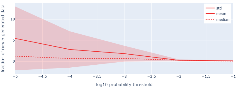
(a) Fraction of new data

(b) Fraction of filtered data

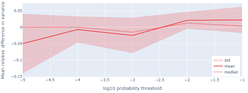
(c) Relative difference in variance with augmentation

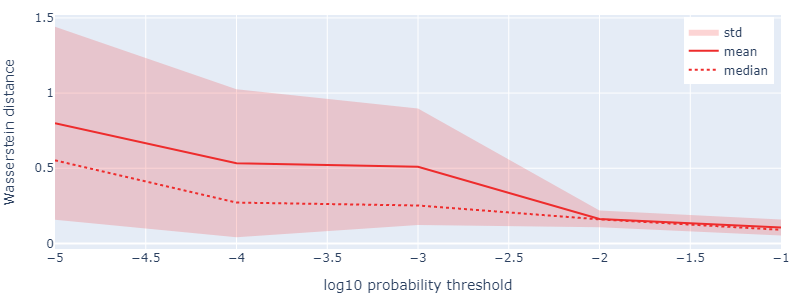
(d) Wasserstein distance, original vs augmented sets

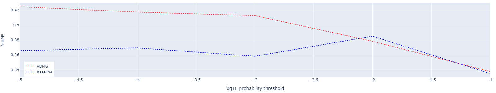
(e) xgb median MAPE score

Figure 1:  CausalDA output characteristics depending on the probability threshold

Inadequate parametrization.

CausalDA relies on its probability threshold parameter $\theta\in{}[0,1]$ (Section 2) to prune the augmented data, which affects their distribution. While a probability threshold close to one accentuates the correlations of the observed data, a threshold close to zero relaxes them according to the causal graph, thus, generating more data points, as illustrated in Figs. 1(a), 1(b) and 1(d). The fact that the variance decreases with the fraction of newly generated data,Fig. 1(c) vs. Fig. 1(a), shows that CausalDA does not tend to increase diversity in the dataset but changes its distribution in dense areas of the observed set. Hence, for an appropriate choice of probability threshold, we expect CausalDA to improve an ml model predictions on the data support by providing a refined data distribution. Figure 1(e) illustrates this finding. The probability threshold parameter seems to have a very narrow value range to improve the performance of the xgb models. Thus, it must be carefully defined by the practitioners. Indeed, this threshold can be interpreted as the minimal probability of accepting a new value for a variable given its parents. From Eq. 1, one can easily see that ${w}_{{i}}>\theta\implies w_{i}^{j}>\theta,\;\forall j\in[1,d]$. Hence, we encourage practitioners to analyze the distribution of each variable given its parents in order to make an informed choice on the probability threshold to use.

Small-data regime.

Figure 2 shows that CausalDA requires at least 300 observations to improve xgb’s performance. This quantity can be considered “relatively high” given the study scenario: (a) no outliers, (b) use of the correct causal graph, (c) in-distribution, (d) data generated from gmm, and (e) neural networks without high discontinuity or divergence . Hence, improving some ml model predictions with CausalDA in a small-data regime may be challenging. One can explain it by observing in Eq. 1 that the kernel density estimator overfits when there are only a few data points. Likewise, because each new data point is generated conditioned on the values taken by its parents, CausalDA needs several observed points with the same parents’ realizations to generate new ones. Hence, we recommend considering CausalDA not as a solution to compensate for the lack of data but rather as a method to refine the estimation of the data distribution via weighted data augmentation.

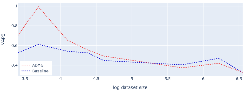
(a) Median MAPE score

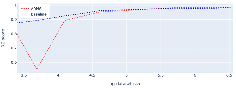
(b) Median R2 score

Figure 2: XGBoost median performance depending on the size of the dataset

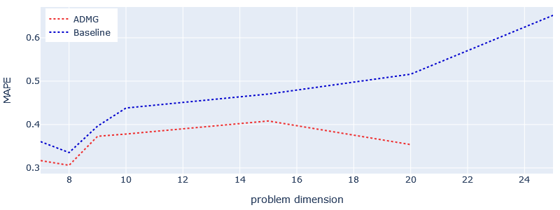
(a) Median xgb’s MAPE score

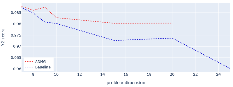
(b) Median xgb’s R2 score

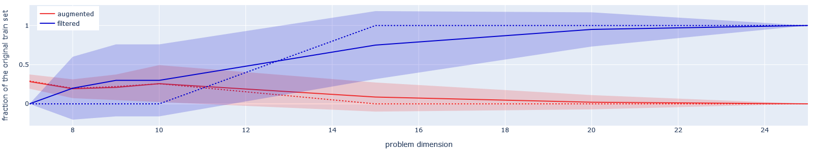
(c) Fraction of new and filtered data points, continuous line is mean, dashed line is median

Figure 3:  CausalDA performances depending on problems dimension

High-dimension scenario.

Figure 3 shows that increasing dimension favors CausalDA. Indeed, CausalDA takes advantage of the prior knowledge about the conditional independence encoded in the causal graph to improve ml models’ generalization. The literature has shown that such a problem is a challenge in low-dimensional data (Shah & Peters (2020)) because high-dimensional settings with a known causal graph and expected degree lead to more conditional independence. Figure 3 also emphasizes that increasing the dimension increases the probability for the whole dataset to be filtered. Indeed, the probability threshold can be interpreted as follows: For a given ${Z}_{i}$, under the hypothesis that all the $w_{i}^{j}$ are equal to $c$, $\sqrt[d]{\theta}$ is the minimum value of $c$ for ${Z}_{i}$ not to be pruned. As $\sqrt[d]{\theta}$ increases with $d$, the higher the dimension, the higher the probability of the weights not to be pruned for a fixed probability threshold. As a result, practitioners also have to consider the dimension of the problem when choosing an appropriate probability threshold value.

Noisy acquisition procedure.

At first sight, we could expect CausalDA to be robust to outliers thanks to its pruning strategy. Indeed, for a high enough probability threshold, the method can theoretically filter outliers with a low probability. However, even in the best-case scenario where all outliers are filtered, they are still taken into account by the Kernel density estimator, making them corrupted and spreading the effect of the outliers on the augmented set. Hence, the robustness of CausalDA to outliers stays an open question. From Fig. 4, it can be seen that CausalDA propagates the outliers to the augmented set degrading xgb’s performance.

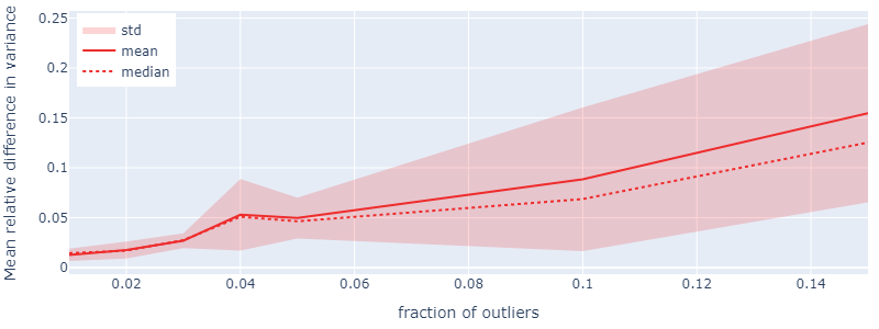
(a) Relative difference in variance adding outliers

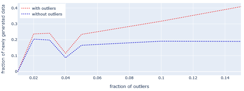
(b) Median fraction of new data

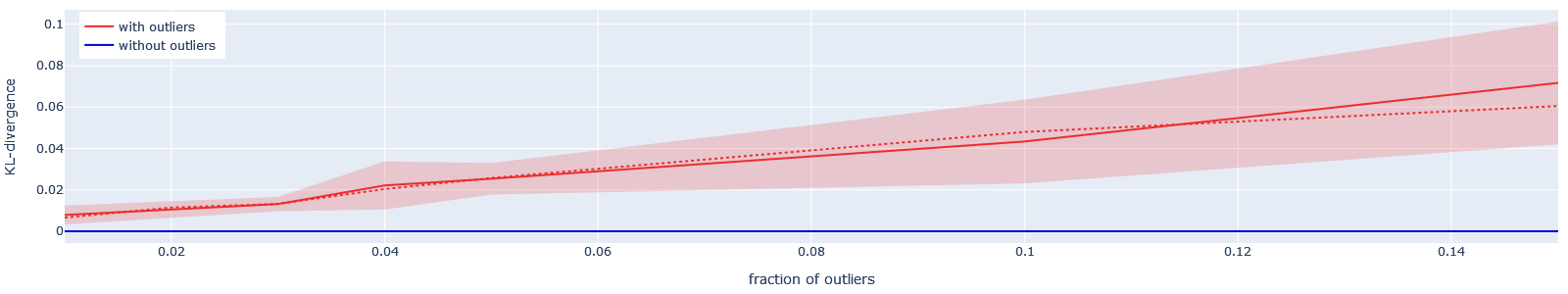
(c) KL-divergence, corrupted vs normal sets, continuous line is mean, dashed line is median

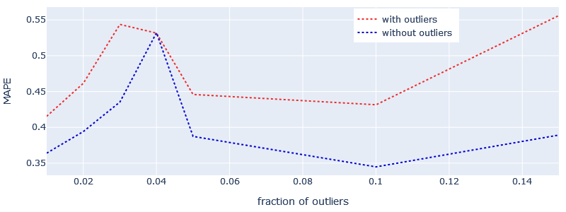
(d) Madian xgb’s MAPE score

(e) Median xgb’s R2 score

Figure 4: CausalDA performances under different level of outlier noise

Discussion.

The results presented in this section enabled us to understand under which conditions CausalDA can help practitioners improve their ml models. First, we observed that CausalDA performance is independent of the underlying causal generation process. Nevertheless, it depends on the acquisition procedure because it is sensitive to outliers. Second, based on our experiments, the method requires at least 300 samples, making it unsuitable for small-data regimes. It can instead be used to improve the generalization of a ml model by providing a more refined data distribution, faithful to the observed one without increasing the diversity, using the prior knowledge encoded in the causal graph. Third, CausalDA highly relies on the probability threshold parameter whose choice might be complex for practitioners. Indeed, up to now, no procedure has been developed to ensure a more guided choice for this parameter. We estimate that this last point is the most critical for practitioners to use this method in real-world use cases. That is why we would like to focus our future work on automating the choice of the probability threshold. Possible solutions include using the ml model to be trained to adjust this parameter automatically or employing mcts (Kocsis & Szepesvári, 2006) when computing the weights instead of the pruning procedure. Also, let us highlight that the experiments of this paper are not self-sufficient. Thus, we would like to deepen our evaluation by, first, using conditional independence tests to check if  CausalDA indeed increases the conditional independences encoded in the causal graph, second, evaluating the method on real data, and third, analyzing the sensitivity to an erroneous causal graph. Indeed, building a causal graph might be challenging and, as far as we know, there is no general procedure to validate its truthful.

5 Conclusion and Further Works

Data scarcity is a significant challenge when applying ml in high-stake domains such as healthcare and finance. Over the last few years, various approaches have been developed to enable researchers and practitioners to increase the size of their datasets artificially and, consequently, the robustness and generalization of their ml models. Causal data augmentation strategies aim to handle these endeavors by relying on conditional independence encoded in a causal graph.

This paper experimentally analyzed the acyclic-directed mixed graph data augmentation method (Teshima & Sugiyama, 2021) considering several scenarios. The goal was to help researchers and practitioners understand under which conditions their prior knowledge help in generating new data that enhance the performance of their models, as well as the influence of the parameters of the data augmentation strategy underneath the presence of outliers, error measures (i.e., aleatoric uncertainty), and the minimal number of samples of the observed data. Experimental results showed that the sample size is essential when employing the method. Likewise, it propagates the outliers when presented in the data. Furthermore, its hyperparameters must be carefully defined for each dataset. In future work, we plan first to carry out further experiments using, notably, conditional independence tests and real data and, secondly, to automatize the hyperparameters optimization process.

Appendix A Appendix

A.1 Non-linear data generation scenario – results

As CausalDA only computes the densities, see Eq. 1, the type of mechanisms linking the variables should not affect the performances of the method, which is illustrated by Fig. 5. Indeed, what matters the most is whether a variable is continuous or discrete because it will affect the choice of the Kernel to use. Moreover, each practitioner can decide to choose a different Kernel based on the distribution of the variables given their parents. A common choice is to use a Gaussian Kernel with a Silverman bandwidth for continuous variables and the identity Kernel for the discrete ones.

Hence, CausalDA can be used in non-linear settings without special care.

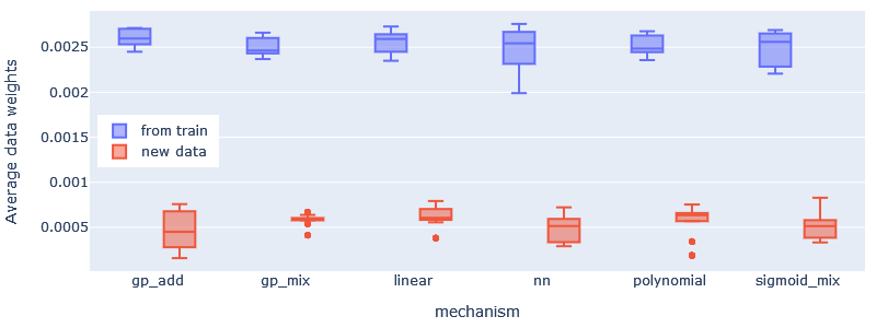
(a) Average weights of the augmented dataset

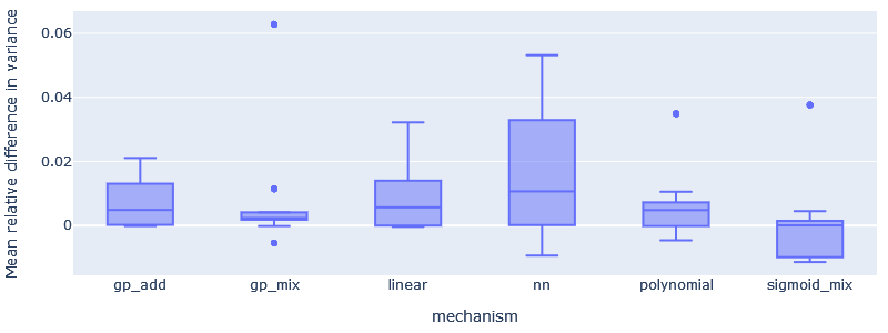
(b) Relative difference in variance with augmentation

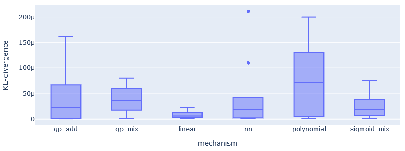
(c) KL-divergence, augmented vs original sets

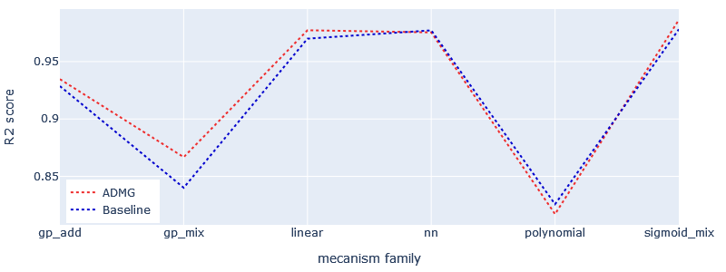
(d) Median xgb’s R2 score

Figure 5:  CausalDA performance under different underlying mechanisms

A.2 Highly dependent input variables scenario – results

From Fig. 6, it can be observed that the more dependent the input variables, the closer to the baseline CausalDA. Looking at the equations from Section 2, this is logical. Indeed, increasing the causal graph density implies that, on average, the number of parents also increases. As a result, the densities are computed on higher dimension supports, making them much smaller and more diluted, which does not encourage the generation of new samples.

In other words, as CausalDA aims to use the conditional independencie induced by the causal graph; if the number of edges increases, the number of conditional independence decreases, making thus the method less useful because it has less prior knowledge to use.

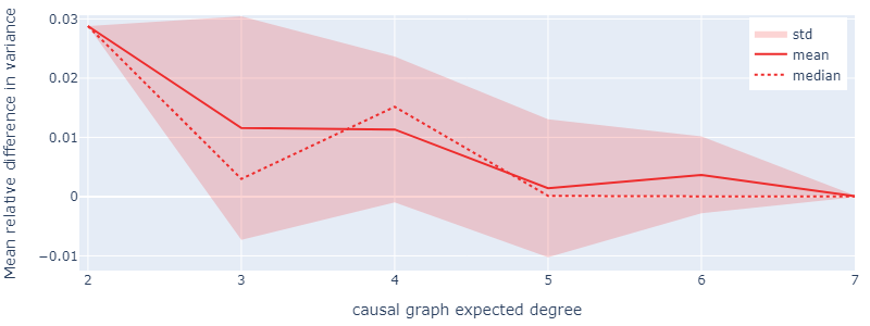
(a) Relative difference in variance with augmentation

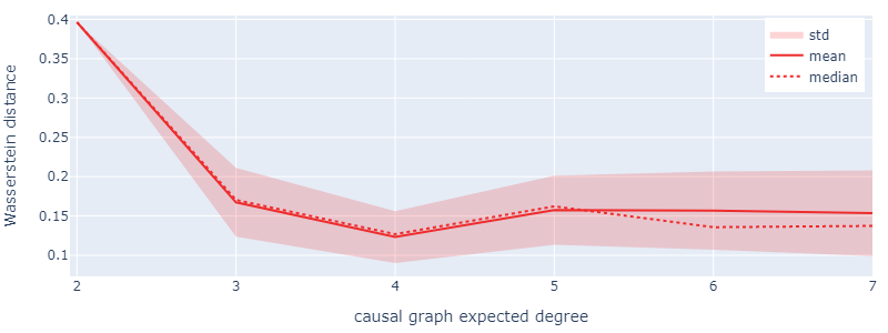
(b) Wasserstein distance of the augmented vs. original sets

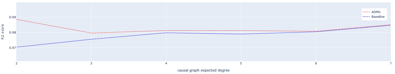
(c) Median xgb’s R2 score

Figure 6:  CausalDA performance under different levels of connectivity in the cg

A.3 Aleatoric uncertainty – results

Based on the results from Fig. 7, it can be asserted that the amplitude of the noise introduced in the scm generating the data does not have a significant influence on the results of CausalDA. This makes sense. Indeed, varying the amplitude of the scms’ noise will only have an effect of scale on the density distributions which could easily be compensated by the bandwidth of the Gaussian kernels automatically optimized with the Silverman formula.

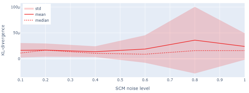
(a) KL-divergence, augmented vs original sets

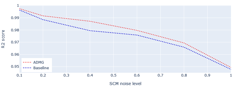
(b) Median xgb’s R2 score

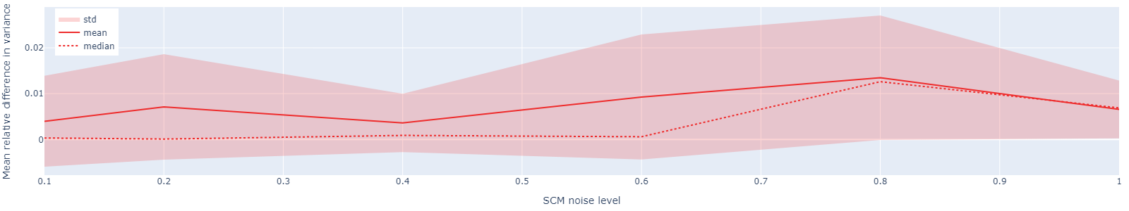
(c) Mean relative difference in variance with augmentation

Figure 7:  CausalDA performance under different level of aleatoric uncertainty

A.4 Causal Discovery Toolbox – AcyclicGraphGenerator module description

Causal Discovery Toolbox (Kalainathan et al., 2020; 2022) is a Python package for causal inference. It mainly focuses on causal discovery in the observational setting. However, this section is dedicated to the description of the AcyclicGraphGenerator module we used for our experiments.

The AcyclicGraphGenerator module is able to randomly generate a scm associated with a dataset. The generator provides the user the ability to choose which mechanism to be used in the data generation process as well as the type of noise contribution (additive and/or multiplicative).

Currently, the implemented mechanisms are:

• Linear: $y=\mathbf{X}W+\times E$

  • $W\sim{\mathcal{U}[0,1]}^{D}$

• Polynomial: $y=\sum_{i=0}^{d}\mathbf{X}^{i}W_{i}+\times E$

  • $d$ the degree

  • $W_{i}\sim{\mathcal{U}[0,1]}^{D}\;\;\forall i$

• Gaussian Process: $y=\sum_{i=0}^{D}s_{i}+\times E$ with and

  • $D$ the number of causes

  • $s_{i}\sim\mathcal{N}(0,cov(\mathbf{X}_{i}))\;\;\forall i$

• Sigmoid: $y=\sum_{i=1}^{D}(1+a)\cdot\frac{b\cdot(\mathbf{X}_{i}+c)}{1+|b\cdot(\mathbf{X}_{i}+c)|}+\times E$

  • $D$ the number of causes

  • $a\sim Exp(4)$

  • $b\sim\tilde{b}\cdot\mathcal{U}[-2,-0.5]+(1-\tilde{b})\cdot\mathcal{U}[0.5,2],\;\tilde{b}\sim Ber(0.5)$

  • $c\sim\mathcal{U}[-2,2]$

• Randomly initialized Neural network: $y=\sigma((\mathbf{X},E)W_{in})W_{out}$

  • $\sigma$ the hyperbolic-tangent activation function

  • $W_{in}$ and $W_{out}$ randomly initialized with the Glorot uniform

with $+\times$ denoting either addition or multiplication, $\mathbf{X}$ the vector of causes of dimension $D$, and $E$ the noise variable accounting for all unobserved variables. As mentioned in Section 3, $E\sim\mathcal{N}(0,1)$ in our experiments.

To generate a random scm associated with a dataset, one needs to specify:

• the functions family of the mechanisms

• the type of noise to use in the generative process (either “uniform” for a $\mathcal{U}[-2,2]$ or “gaussian” for a $\mathcal{N}(0,1)$ )

• the proportion of noise in the mechanism

• the number of observations to generate

• the number of nodes/variables in the structural causal model

• the type of dag to generate (either ’default’ to be sampled from the default procedure or “erdos” to be sampled from the Erdös-Rényi model (Erdös & Rényi, 1959) augmented with a conditioned on the new sampled edges to check if it does not lead to a cycle)

  • if “default“: a maximum number of parents per node has to be specified

  • if “erdos”: an expected degree for the dag has to be specified

Then, each scm is generated according to the following procedures:

1. The dag is generated

2. The mechanism functions are generated

3. The source variables (i.e., vertices without a parent in the causal graph) are generated using GMMs with four components and with a spherical covariance.

4. Noise variables are introduced into the causal mechanisms. They are all i.i.d.

Once a scm is built, the data are generated by sampling the realizations of the source and the noise variables. Next, the mechanism functions compute the realizations of the variables following the topological order of the dag.

A.5 Experiments’ default parameters

Table 1: Parameters’ values when not under study

Parameter	Value
Network architecture	2-layers fully-connected neural network with hyperbolic tangent activation function and 20 neurons initialized through the Glorot uniform
Number of variables	10
Causal graph expected degree	3
Additive noise amplitude	0.4
Probability threshold	$10^{-2}$
Fraction of outliers	0
Number of repetitions	20
Kernels function	Gaussian Kernels with Silverman bandwidth

References

- Alaa et al. (2022) Ahmed Alaa, Boris Van Breugel, Evgeny S Saveliev, and Mihaela van der Schaar. How faithful is your synthetic data? sample-level metrics for evaluating and auditing generative models. In International Conference on Machine Learning, pp. 290–306, 2022.
- Chickering (1996) David Maxwell Chickering. Learning bayesian networks is np-complete. Learning from data: Artificial intelligence and statistics V, pp. 121–130, 1996.
- Chickering et al. (2004) Max Chickering, David Heckerman, and Chris Meek. Large-sample learning of bayesian networks is np-hard. Journal of Machine Learning Research, 5:1287–1330, 2004.
- Erdös & Rényi (1959) P. Erdös and A. Rényi. On random graphs i. Publicationes Mathematicae Debrecen, 6:290–297, 1959.
- Hao et al. (2023) Xiaoshuai Hao, Yi Zhu, Srikar Appalaraju, Aston Zhang, Wanqian Zhang, Bo Li, and Mu Li. MixGen: A new multi-modal data augmentation. In IEEE/CVF Winter Conference on Applications of Computer Vision, pp. 379–389, 2023.
- Hendrycks et al. (2021) Dan Hendrycks, Steven Basart, Norman Mu, Saurav Kadavath, Frank Wang, Evan Dorundo, Rahul Desai, Tyler Zhu, Samyak Parajuli, Mike Guo, et al. The many faces of robustness: A critical analysis of out-of-distribution generalization. In IEEE/CVF International Conference on Computer Vision, pp. 8340–8349, 2021.
- Ilse et al. (2021) Maximilian Ilse, Jakub M Tomczak, and Patrick Forré. Selecting data augmentation for simulating interventions. In International Conference on Machine Learning, pp. 4555–4562, 2021.
- Kalainathan et al. (2020) Diviyan Kalainathan, Olivier Goudet, and Ritik Dutta. Causal Discovery Toolbox: uncovering causal relationships in Python. The Journal of Machine Learning Research, 21(1):1406–1410, 2020.
- Kalainathan et al. (2022) Diviyan Kalainathan, Olivier Goudet, Isabelle Guyon, David Lopez-Paz, and Michèle Sebag. Structural agnostic modeling: Adversarial learning of causal graphs. Journal of Machine Learning Research, 23(219):1–62, 2022.
- Kocsis & Szepesvári (2006) Levente Kocsis and Csaba Szepesvári. Bandit based monte-carlo planning. In 17th European Conference on Machine Learning, pp. 282–293, 2006.
- Little & Badawy (2019) Max A Little and Reham Badawy. Causal bootstrapping. arXiv:1910.09648, 2019.
- Pearl (2009) Judea Pearl. Causal inference in statistics: An overview. Statistics surveys, 3:96–146, 2009.
- Richardson (2003) Thomas Richardson. Markov properties for acyclic directed mixed graphs. Scandinavian Journal of Statistics, 30(1):145–157, 2003.
- Shah & Peters (2020) Rajen D. Shah and Jonas Peters. The hardness of conditional independence testing and the generalised covariance measure. The Annals of Statistics, 48(3):1514 – 1538, 2020.
- Talavera et al. (2022) Edgar Talavera, Guillermo Iglesias, Ángel González-Prieto, Alberto Mozo, and Sandra Gómez-Canaval. Data augmentation techniques in time series domain: a survey and taxonomy, 2022.
- Teshima & Sugiyama (2021) Takeshi Teshima and Masashi Sugiyama. Incorporating causal graphical prior knowledge into predictive modeling via simple data augmentation. In Uncertainty in Artificial Intelligence, pp. 86–96, 2021.
- Van Dyk & Meng (2001) David A Van Dyk and Xiao-Li Meng. The art of data augmentation. Journal of Computational and Graphical Statistics, 10(1):1–50, 2001.
- Wen et al. (2021) Qingsong Wen, Liang Sun, Fan Yang, Xiaomin Song, Jingkun Gao, Xue Wang, and Huan Xu. Time series data augmentation for deep learning: A survey. In Thirtieth International Joint Conference on Artificial Intelligence, 2021.
- Xie et al. (2020) Qizhe Xie, Zihang Dai, Eduard Hovy, Thang Luong, and Quoc Le. Unsupervised data augmentation for consistency training. Advances in neural information processing systems, 33:6256–6268, 2020.
- Zhong et al. (2020) Zhun Zhong, Liang Zheng, Guoliang Kang, Shaozi Li, and Yi Yang. Random erasing data augmentation. AAAI Conference on Artificial Intelligence, 34(07):13001–13008, 2020.