A Machine Learning Approach to Forecasting Honey Production with Tree-Based Methods

Abstract

The beekeeping sector has undergone considerable production variations over the past years due to adverse weather conditions, occurring more frequently as climate change progresses. These phenomena can be high-impact and cause the environment to be unfavorable to the bees’ activity. We disentangle the honey production drivers with tree-based methods and predict honey production variations for hives in Italy, one of the largest honey producers in Europe. The database covers hundreds of beehive data from 2019-2022 gathered with advanced precision beekeeping techniques. We train and interpret the machine learning models making them prescriptive other than just predictive. Superior predictive performances of tree-based methods compared to standard linear techniques allow for better protection of bees’ activity and assess potential losses for beekeepers for risk management.

Keywords: machine learning, honey, prediction, pollinators, weather.

JEL classification codes: C33, C53, O13, Q54.

1 Introduction

Honeybees, Apis mellifera L. species, are essential insects, playing a vital role in human society and contributing to the food system through pollinating numerous crops. Pollinators improve the production of 70% of the globally most important crop species and, although the main cereal staple food is self-pollinated, influence 35% of the global human food supply (Tscharntke et al., 2012). The estimated annual economic value of honeybee pollination is in the order of billions, especially due to the key role in enhancing agriculture production and ensuring plant reproduction (Delaplane et al., 2000; Millennium Ecosystem Assessment (2005), MEA; Klein et al., 2007; Garibaldi et al., 2014; Food and Agriculture Organization of the United Nations (2018), FAO). Therefore, the decline in honey production threatens food security, as less pollination leads to a reduced crop yield. Besides their role in crop pollination, honeybees are essential producers of honey, which is widely consumed for its health benefits. Honey production contributes to the economy, with the global honey market that was estimated to amount to over 8 billion in 2021.

With 20 million beehives and 218000 tons in 2022, the European Union is the second largest honey producer after China. However, the former also imports a surplus of around 40% of the amount of honey produced to cover domestic consumption, making imports greater than exports. The largest honey production is mainly located in Southern Europe, where climatic conditions are more favorable to beekeeping, as reported by the European Commission.

Honey production depends on three major categories: climate, pests and diseases, and beekeeping practices. For instance, honeybees need adequate forage and water to produce honey, and a lack of either can result in reduced production. Additionally, changes in temperature and rainfall patterns can affect flower blooming, leading to a decline in nectar and pollen production. Pests and diseases like Varroa mites can also affect honey production. Varroa mites are external parasites that feed on honeybees, leading to a weakened immune system and increased susceptibility to diseases. The use of pesticides and insecticides in agriculture also contributes to the decline in honeybee populations, as they can kill bees and disrupt their behavior. Beekeeping practices can also influence honey production. Proper hive management, such as regular inspections and adequate feeding, can increase honey production. On the other hand, poor management practices, such as overcrowding and improper ventilation, can lead to hive diseases and a decline in honey production.

In this paper, we approach the study of honey production drivers by focusing specifically on the climate effect. It is undoubtedly clear that climate change will cause major modifications to the depicted framework of honey production (Holmes, 2002; Gordo and Sanz, 2006; Le Conte and Navajas, 2008; Switanek et al., 2017; Flores et al., 2019; Solovev, 2020; Calovi et al., 2021). Due to its geographical collocation, Italy is one of the most affected countries as Italian beekeepers recorded substantial variations in honey production with losses up to 70% in some regions (Porrini et al., 2016; Gray et al., 2019). It is essential to understand the climate aspects to get insights into the beekeeping system’s efficiency to decrease the risk of losses and maximize their activity’s social output. Extended periods of rain and sudden temperature increases have disastrous impacts on spring plants and bees’ health, implicitly causing an impact on total honey production.

The paper’s contribution is twofold: detecting the drivers for better forecasting of honey production is a quantitative tool that beekeepers can leverage to manage their activity. In addition, it can also help mitigate the risk associated with sudden losses. This analysis can also be a powerful tool for effective beekeeping risk management in the hand of insurance companies that can build machine learning-informed insurance products to protect beekeepers from massive losses. The predicted variation of honey production can be practically used to determine crucial decisions in honey bee cultivation, such as where and when to move the beehive geographically to avoid adverse weather events. Such a task became possible in recent years due to the technological advancements that allow tracking beehive characteristics and collecting large amounts of data to be analyzed. Apiculture activities, the technical term for beekeeping, profited from introducing precision beekeeping technologies, a precision agriculture branch (Zacepins et al., 2012), focused on the apiary management strategy by monitoring individual bee colonies through connected smart devices.

Our analysis leverages the data from a technology company, 3BEE S.R.L.. The company develops intelligent monitoring and diagnostic systems for bee health, bringing together numerous beekeepers. The analyzed dataset comprises over forty million records from about 500 bee hives across Italy. Then we integrate the beehive characteristics with weather features from the open-source database named Copernicus (Muñoz Sabater, 2021; Muñoz Sabater et al., 2019) to capture the effect of the surrounding climate variation on honey production and tackle the forecasting problem effectively.

We perform the forecasting problem using two different tree-based methods, Random Forest (RF) (Breiman, 2001) and Extreme Gradient Boosting (XGB) (Chen and Guestrin, 2016), ensembles of regression trees (Breiman et al., 1984) able to detect the nonlinear patterns in our collected data. The choice of tree-based models relies on the trade-off between forecasting power, improving on more classical linear methods used for statistical analyses, and explainability, allowing us to produce a more meaningful feature importance analysis compared to other families of machine learning models such as neural networks. The former capability of tree-based methods allows us to extract insights from the data and give the users of the predictive model a higher degree of confidence in the results provided. Therefore, the output of the analysis is a model that becomes prescriptive other than just predictive, informing decisions regarding the risk management aspect of the honeybees industry.

1.1 Related Literature

The effect of weather and environment on beehive weight variations has been known for over a century (Hambleton, 1925). Many works relate the influence of seasonal weather conditions on honey productivity and the health conditions of bees. Szabo (1980) find a positive correlation between the bees’ flight activity and the temperature, Holmes (2002) regress up to 21 variables related to honey production. Bhusal and Thapa (2006) study honey production based on the Randomized Complete Block, a common technique in the agriculture field to control for the driving factor of the production. Flores et al. (2019); Gounari et al. (2022); Catania and Vallone (2020) provide a more recent outlook on climate change impacts on bees’ activity in the Mediterranean area. Over the years, the evolution of technologies and data availability allowed the development of sophisticated statistical methods for studying bees’ behavior, pollen foraging, and weather impact. Clarke and Robert (2018) investigate the relationship between the foraging activity of honey bees and local weather conditions in the United Kingdom with generalized least squares, whereas Karaboga and Ozturk (2011) implement a cluster analysis for simulating the intelligent foraging behavior of a honey bee swarm. Another estimation based on a cluster analysis is carried out by Nasr et al. (2014). Overturf et al. (2022) conduct a Canada-based research highlighting the close correlation between winter weather and honey losses with standard regression and spatial analysis. Becsi et al. (2021) present a novel approach to quantify the effects of weather conditions on Austrian honey bee colony winter mortality by defining biophysics-based weather indicators. Dainat et al. (2012) study the spreading of Varroa infestation and consequent high mortality of bees has been correlated to temperature conditions.

Besides the use of classical statistical methods, other works estimate honey production through spatial regression (Tassinari et al., 2013), fuzzy inference methods (Hastono et al., 2017) Other papers resort to the estimation of honey production based on innovative procedures (Bhusal and Thapa, 2006; Hastono et al., 2017), clustering algorithms (Rafael Braga, G. Gomes, M. Freitas and A. Cazier, 2020), K-Nearest Neighbor (Yesugade et al., 2018), Tree-based methods (Calovi et al., 2021; Quinlan et al., 2022; Rafael Braga, G. Gomes, Rogers, E. Hassler, M. Freitas and A. Cazier, 2020). Karadas and Kadirhanoğulları (2017) aim to determine relevant factors influencing average honey yield per beehive. For this purpose, the predictive performances of several data mining algorithms and neural networks were compared. Alves et al. (2020) adopt convolutional neural networks to detect cells in comb images and classify their contents into seven classes, distinguishing into cells occupied by eggs, larvae, capped brood, pollen, nectar, and honey. Campbell et al. (2020) use regression trees to estimate the honey harvests in South West Australia based on weather and vegetation-related information obtained from satellite sensors. Ngo et al. (2021) show the correlation between environmental data and pollen foraging with a neural network-powered imaging system, emphasizing that temperature, relative humidity, wind speed, rain level, and light intensity influence colony activity.

Although the use of tree ensembles is not new to the field of honeybee analysis, an analysis of the Italian territory is still missing. We believe is crucial to gain an in-depth understanding of the driver of honey production in Italy by leveraging the predictive power and the explainability of these methods.

The rest of the paper is organized as follows. Sec. 2 describes the data collection and the dataset structure from different sources. Then the data are further preprocessed as explained in Sec. 3 to prepare the data before the model estimation. Sec. 4, describes the model results and their interpretation via feature importance analyses. The final Sec. 5 summarizes the results and highlights further improvements.

2 The Databeese

The precision beekeeping branch of agriculture is expanding to minimize resources and maximize the productivity of bees through connected smart beehives (Catania and Vallone, 2020; Anwar et al., 2022; Hadjur et al., 2022). Thanks to these tracking technologies and the voluntary involvement of beekeepers as key collaborators, gathering a large amount of data related to hives conditions has become possible. We also complement the beehive information with meteorological data spread throughout the Italian territory. Hereafter, we refer to the database combining the two sources with the word pun Databeese.

The beehives dataset originates from 3BEE S.R.L, an agri-tech company that develops devices for intelligent monitoring and bee health diagnostic systems. Through their technology, beekeepers can fully monitor their hives to gather real-time information that optimizes production by preventing issues and diseases. At the time of writing, the company has developed a network of 10000 beekeepers throughout Italy. Among those that agreed to provide the data for research purposes, we obtained data relative to 512 of those hives over the period 2019-2022. A visualization of the geographical position of those hives is available in Fig. 1.

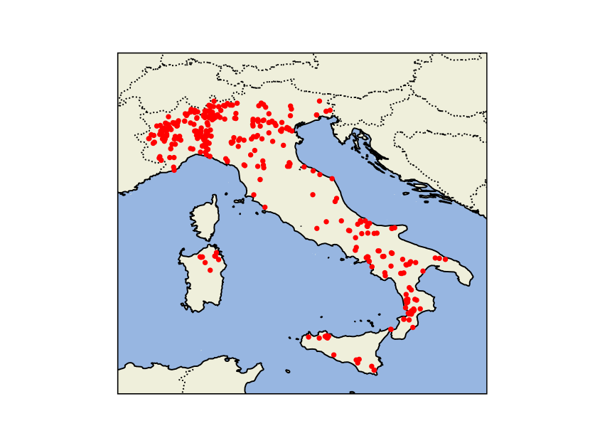
Figure 1: Geographical distribution of the hives over the Italian territory.

Beehives are monitored through sensors that can transmit information such as the geolocation (latitude and longitude) and the weight of the respective hive. In this way, we form a panel dataset of hives’ time series from January 2019 to July 2022. The panel is unbalanced since not all the beekeepers adopted the company’s program at the same time, and precision beekeeping is relatively novel for the Italian beekeeping landscape.

As a first step, data for each hive have been resampled to the daily frequency by taking the average weight measured over the course of a single day. This choice solves the problem of measurement errors and missing records within a given day. It allows us to focus the analysis on a robust proxy of honey production, such as the hive’s weight since an increase in honey production will obviously increase the whole structure. In this regard, we want to specify that the scale apt to weigh the hive measures the total weight, including the amount of honey produced, the bees, and the wood structure that contains and protects the hive itself. Such hive structure varies from $23$ to $30\;$\mathrm{k}\mathrm{g}$$, while an additional structure is added on top during the harvest seasons, adding around $7\;$\mathrm{k}\mathrm{g}$$ in total. After filtering for missing values and recording errors, we remain with 431 hives in our DataBeese.

For each reported hive location, we also obtained daily weather data from a $$9\text{\,}\mathrm{k}\mathrm{m}$-$gridded reanalysis weather model (Muñoz Sabater et al., 2021; Muñoz Sabater et al., 2019; Muñoz Sabater, 2021) with a method that associates every hive location with a weighted average in altitude and distance of the weather features values in the model cells up to $20\text{\,}\mathrm{k}\mathrm{m}$ from the hive. In such a way, we have a variety of climate-based characteristics as reported in Tab. 1 with their respective unit of measure.

Variable	Unit	Average	Std Dev	$P_{0}$	$P_{25}$	$P_{50}$	$P_{75}$	$P_{100}$
Average Hive Weight	Kg	34.11	15.68	0.01	26.87	32.11	39.92	1284.74
Latitude	d.d.	43.62	2.61	36.83	41.50	44.98	45.54	46.31
Longitude	d.d.	11.07	3.15	7.09	8.59	9.60	14.17	17.54
Average Temperature 2 m.a.g.	$\mathrm{\SIUnitSymbolCelsius}$	13.23	7.85	-20.37	7.02	12.67	19.91	33.66
Max Temperature 2 m.a.g.	$\mathrm{\SIUnitSymbolCelsius}$	17.50	8.18	-12.42	11.12	16.87	24.10	41.93
Min Temperature 2 m.a.g.	$\mathrm{\SIUnitSymbolCelsius}$	8.88	7.58	-28.00	2.77	8.73	15.18	28.82
Max Rainfall	$\mathrm{m}$	0.51	1.01	-0.00	0.00	0.07	0.53	13.62
Total Rainfall	$\mathrm{m}$	2.69	6.69	0.00	0.00	0.22	2.09	150.77
Average Dewpoint Temperature	$\mathrm{K}$	7.63	7.04	-27.11	2.39	8.15	13.37	23.55
Average Wind Speed	$\mathrm{m}$ $$\mathrm{s}$^{-1}$	1.68	1.01	0.25	1.04	1.38	1.98	11.55
Average Solar Radiation	J $$\mathrm{m}$^{-2}$	150.13	76.45	0.00	81.28	150.52	218.13	386.22
Average Surface pressure	$\mathrm{P}\mathrm{a}$	964.54	35.81	803.32	946.89	970.96	988.88	1042.11

Table 1: Descriptive statistics of the variables included in the Databeese. The units of measure follow the international system of units (SI).

3 Data Preprocessing

We extensively preprocess the raw variables in Tab. 1 to construct the feature for the predictive models we test in the coming Sections. Our preprocessing is articulated in several steps described in this section.

First, we check for outliers that could weaken the models’ performance since we are aware of possible measurement errors of the hive sensors and usage of reanalysis data, causing problems in the hive characteristics data and the climate measure, respectively. In this light, the target variable for the forecasting problem presents most of the discrepancies in our Databeese. The cleaning task of these time series requires a two-step approach. At first, we address plain measurement errors since some hives show a zero weight, even though we know in advance (see Sec. 2) that an empty hive’s weight must be around between 20 and 30 kg. We removed all the values where the hive weighed less than 20 kg. In addition, to identify sudden variations in the time series of the hive weight that are not strictly related to the time series, we compute a rolling Z-score on a 30 days window on each hive’s time series separately. The threshold for removing significant outliers is 1.2 for each hive-weight time series. Fig. 2 shows a visualization of the two-step data-cleaning procedure for a pair of hives.

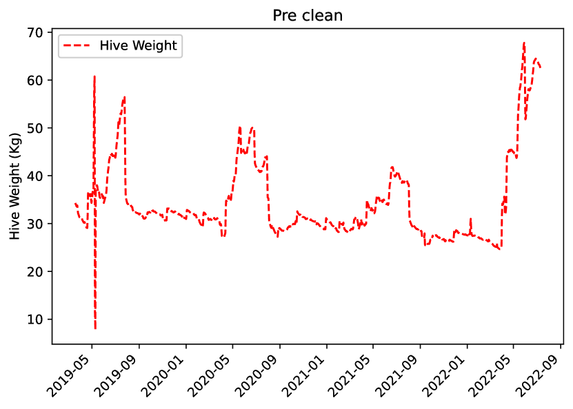
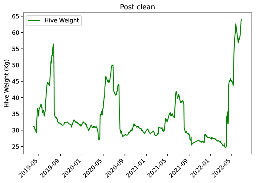
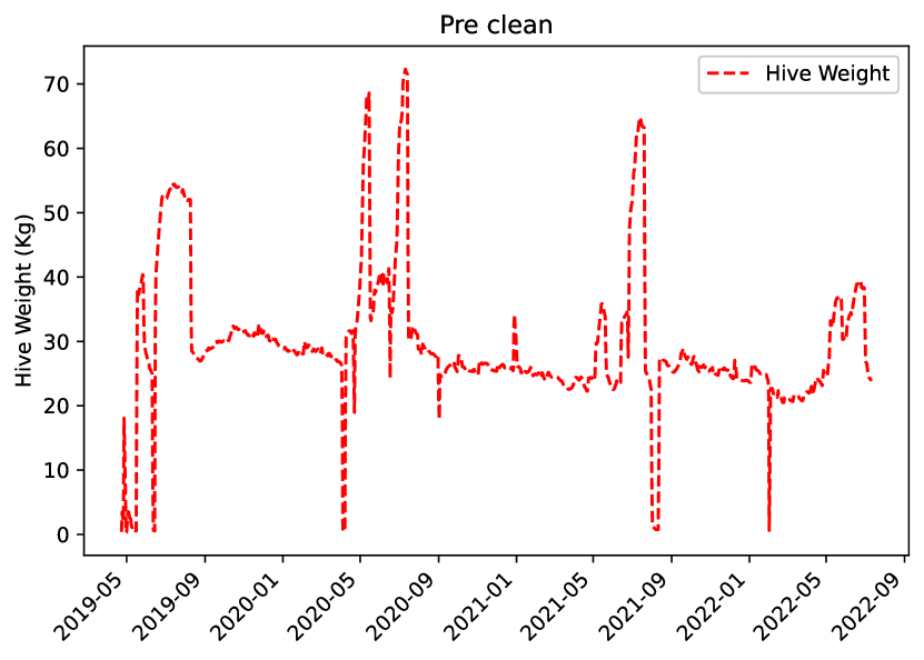
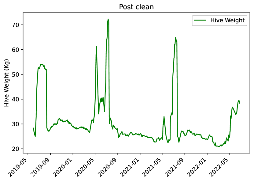
Figure 2: Time series of two hives in training set before (left column) and after (right column) the removal of measurement errors.

As a second step, we ensure that the variables from the raw Databeese are stationary in the mean to avoid the risk of finding spurious patterns. We test all the variables of each hive in a separate manner through the Augmented Dickey-Fuller (ADF) test. When one of the variables is non-stationary, we compute the first difference. Tab. 2 shows the percentage of the absolute-value time series that are non-stationary together with those that are stationary after the differentiation.

Variable	Absolute value % Stationary	Difference % Stationary
Hive weight	20	100
Temperature	1	100
Precipitations	97	100
Wind speed	98	100
Radiation	14	100
Pressure	98	100
Dew point	5	100

Table 2: Percentage of stationary variables in the Databeese. The ADF test is performed on each hive separately and for every variable considered. The reported percentages refer to hives for which the observed series is stationary.

Before proceeding, we also perform an additional check on the hive weight variation, searching for outliers. In addition to the measurement errors, the hives time series presents other irregularities that must be processed. Firstly, when the beekeeper harvests the honey, the variable presents huge negative values unrelated to adverse weather conditions. Secondly, the time series shows several production peaks that are beyond the expected honey production in a day.

We compute a Z-score on the whole time series to remove these values, setting the threshold to 2. As the last step, hives with less than 60 observations are discarded to ensure consistent measurements.

We derive additional feature by lagging the model variables to improve the prediction performance. In particular, we compute the lagged features at $t-1,t-2,t-3$. A complete list of the features with descriptive statistics is provided in the appendix A.

4 Modeling Methodologies

We train and test two tree-based methods, Random Forest (RF) (Breiman, 2001) and Extreme Gradient Boosting (XGB) (Chen and Guestrin, 2016), and compare their result with an OLS-estimated linear regression model as a benchmark for linear modeling approaches. RF and XGB have been popularized for tackling supervised learning problems in various domains. In this section, we recall their main characteristics and highlight their differences. However, they are both ensemble learning methods (Opitz and Maclin, 1999) aggregating the prediction of many weak learners as the regression trees (Breiman et al., 1984)

Regression trees (Breiman et al., 1984) are non-parametric models that partition the input space into a set of rectangular regions and fit a constant value to each region. Given a dataset of $N$ observations, with $p$ inputs and a target variable, denoted as $(x_{i},y_{i})$ for $i=1,2,\ldots,N$, where $x_{i}=\left(x_{i1},x_{i2},\ldots,x_{ip}\right)$, a regression tree aims at determining the optimal splitting variables and points as well as the tree topology. If one assumes to have a partition of the input space into $M$ disjoint regions, denoted as $R_{1},R_{2},\ldots,R_{M}$, the model output within each region $R_{m}$ is a constant $c_{m}$:

$$f(x)=\sum_{m=1}^{M}c_{m}I\left(x\in R_{m}\right).$$ (1)

A regression tree minimizes the sum of squares $\sum_{i=1}^{N}\left(y_{i}-f\left(x_{i}\right)\right)^{2}$ by estimating the optimal value $\hat{c}_{m}$ as the average of $y_{i}$ within each region $R_{m}$:

$$\hat{c}_{m}=\operatorname{ave}\left(y_{i}\mid x_{i}\in R_{m}\right).$$ (2)

To this end, a greedy algorithm searches for the optimal splitting variable $j$ and split point $s$ by minimizing

$$\min_{j,s}\left[\min_{c_{1}}\sum_{x_{i}\in R_{1}(j,s)}\left(y_{i}-c_{1}\right)^{2}+\min_{c_{2}}\sum_{x_{i}\in R_{2}(j,s)}\left(y_{i}-c_{2}\right)^{2}\right]$$ (3)

where $R_{1}(j,s)=\{X\mid X_{j}\leq s\}$ and $R_{2}(j,s)=\{X\mid X_{j}>s\}$ are the two half-planes defined by the splitting variable $j$ and split point $s$. The inner minimization problem for $c_{1}$ and $c_{2}$ is solved using the mean of $y_{i}$ within each half-plane

$$\hat{c}_{1}=\operatorname{ave}\left(y_{i}\mid x_{i}\in R_{1}(j,s)\right)\text{ and }\hat{c}_{2}=\operatorname{ave}\left(y_{i}\mid x_{i}\in R_{2}(j,s)\right)$$ (4)

Once the tree has been constructed, we can use it to predict the output for a new input vector $x_{new}$ by traversing the tree until we reach a leaf node and returning the mean value associated with that node.

RF extend regression trees to ensembles by constructing multiple trees and averaging their predictions. Each tree is trained on a random subset of the input data, and at each split, the algorithm randomly selects a subset of the features. This reduces overfitting by introducing diversity among the trees. When putting together the final prediction, the output of each tree is aggregated to obtain a single value which decreases the prediction’s variance while maintaining the bias stable (Breiman, 2001). One can express the RF for regression as

$$y_{RF}=\frac{1}{M}\sum_{m=1}^{M}f_{m}(x)$$ (5)

where $y_{RF}$ is the predicted value, $M$ is the number of trees in the forest, and $f_{m}(x)$ is the prediction of the $m$-th tree on the input vector $x$.

On the other hand, XGB is a gradient-boosted tree model that sequentially adds new trees to the ensemble, each one correcting the errors of the previous ones. The model is defined as

$$y_{XGB}=\sum_{m=1}^{B}f_{m}(x),\quad f_{m}\in\mathcal{F}$$ (6)

where $\mathcal{F}$ is the space of regression trees, and the tree ensemble is trained sequentially instead of being parallelized as for bagging techniques like RF. The boosting technique (Friedman, 2001) implies that trees are added to minimize the errors made by previously fitted trees until no further improvements are achieved. The optimization procedure builds trees as a forward mechanism, where every step reduces the error of the previous iteration. We initialize the ensemble with a single regression tree and then iteratively add new trees that minimize the error made by the previous tree by gradient descent.

One of the main differences between RF and XGB is their approach to feature selection. RFs use random subsampling of features to prevent overfitting and increase the diversity of the trees. In contrast, XGB uses a gradient-based approach to select the most informative features, which helps to improve the model’s accuracy and efficiency. Another difference is their training time and scalability. RFs can be trained quickly and can handle large datasets with high-dimensional features. However, the performance may degrade if the number of features is much larger than the number of examples. XGB, on the other hand, can handle very large datasets and high-dimensional features by exploiting sparsity and parallel computing. However, the training time may be longer than random forests for small datasets. Generally, the gradient-based optimization approach of XGB is better at capturing complex non-linear relationships between the input features and the target variable than the splitting criteria of each regression tree involved in the RF model. Moreover, the XGB structure focuses heavily on correcting predictions on difficult examples in the dataset. It can also be properly regularized for controlling overfitting rather than relying on randomness and feature subsampling as RF.

Comparing the results of the tree-based methods with a linear regression model allows us to test if our problem can be solved by a simple and well-understood model where the relationship between the feature and target variables is linear in its few parameters. Standard statistical techniques’ high efficiency and interpretability often have reduced forecasting capabilities since they limit themselves to linear patterns. In contrast, more complex and computationally expensive tree-based methods can model more structured nonlinear relationships within the data. given the known trade-off between the complexity and explainability of machine learning models, we provide an extensive feature importance analysis to disentangle the large number of decision rules underneath the tree-based algorithms. Therefore, tree-based methods represent a good choice when the relationship between the input and target variables is complex and nonlinear, as in the case of the variation of the honey production problem.

Empirical Findings

This section provides the evaluation of the model predictions. We adopted two different approaches when training and testing the tree-based methods and their benchmark. We train the model on the whole Databeese, but we also repeat the same experiment by restricting the time period to consider only the period in which bees produce the majority of honey, between March and September.

Using the dataset described, we train the two ensemble models with 5-fold cross-validation methods and fine-tune the hyperparameters through a stochastic search over a large grid. The splitting method in train and test sets follow the hives ID so that 80% of the hive history is used for training and the remaining for testing.

We evaluate the prediction results with different metrics: the coefficient of determination R-Squared ($R^{2}$) to understand how much variability in the target is explained by the model inputs, and both the Mean Squared Error (MSE) and the Mean Absolute Percentage Error (MAPE) to get an absolute and a relative measure of discrepancy from the true weight of the hive.

Model	Dataset	Complete dataset			Production period
		R-Squared	MSE	MAPE	R-Squared	MSE	MAPE
Random Forest	train set	0.505	0.110	10.008	0.526	0.185	7.883
	test set	0.435	0.109	8.713	0.436	0.192	7.552
Gradient Boosting	train set	0.461	0.119	12.239	0.526	0.185	11.737
	test set	0.440	0.108	8.668	0.460	0.184	8.998
Linear Regression	train set	0.299	0.155	21.085	0.351	0.254	8.034
	test set	0.379	0.120	11.075	0.393	0.206	10.325

Table 3: Results of the models’ prediction performance. Linear regression is added for comparison.

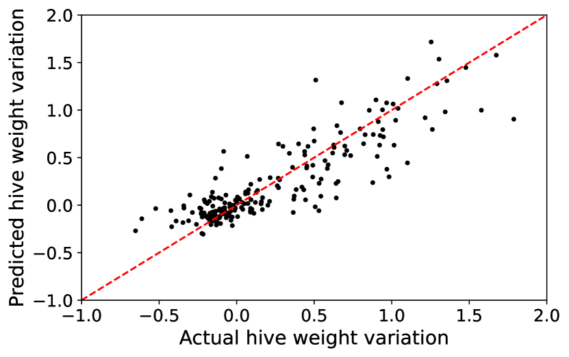
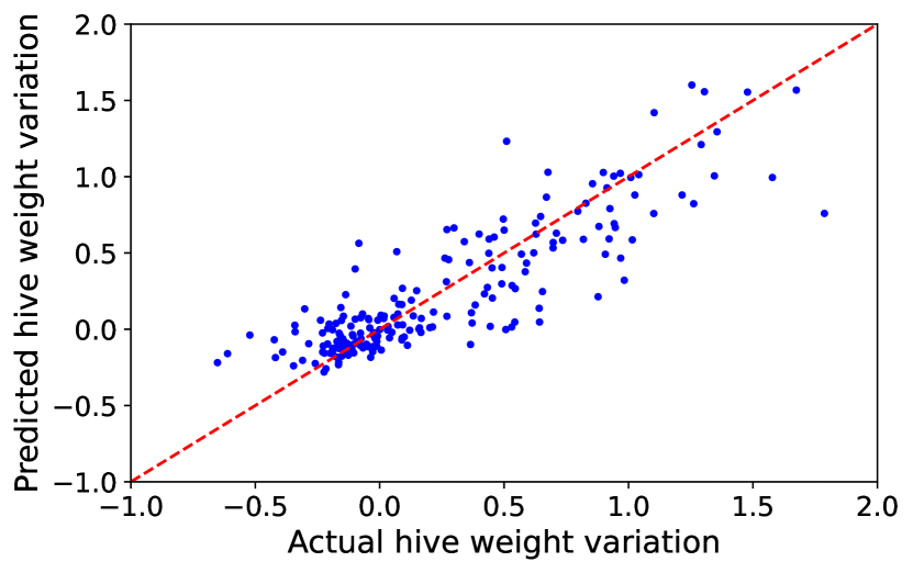
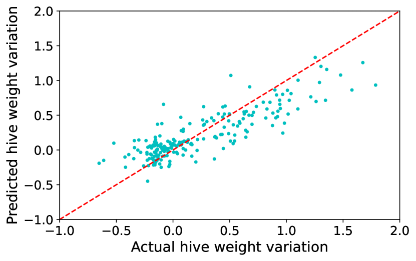
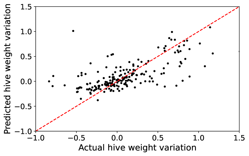
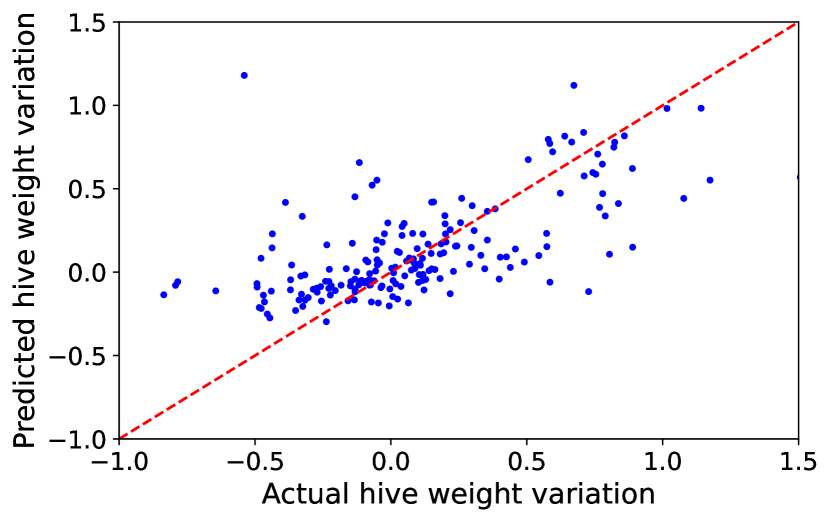
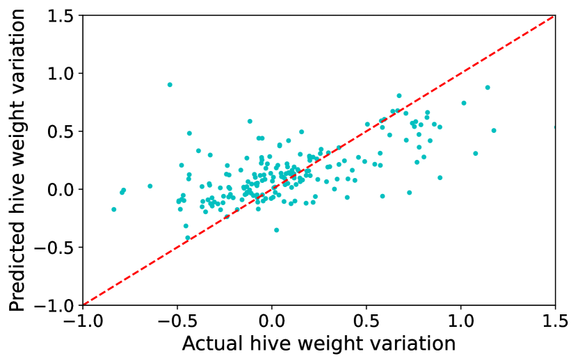
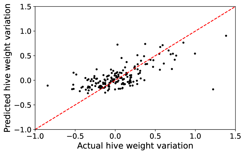
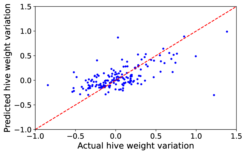
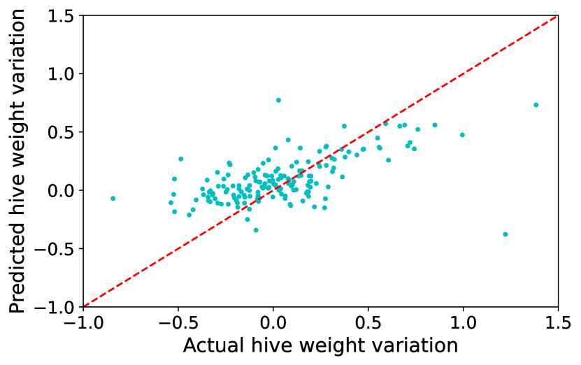
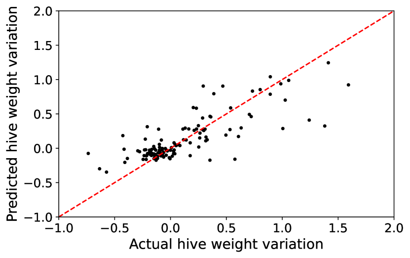
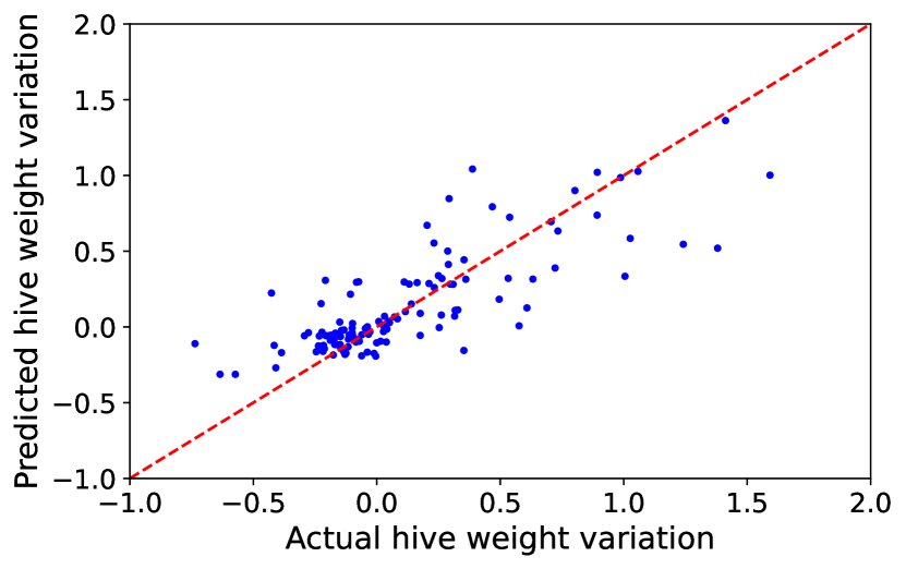
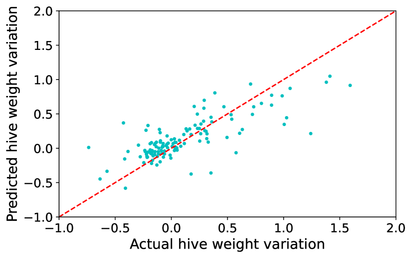
Figure 3: Scatter plot of actual (x-axis) vs. predicted (y-axis) variation in hive weights for 4 different hives in the test set. Each row represents a different hive, while the columns refer to XGB, RF, and linear regression in this order. The red bisector of the first quadrant angle in every subplot helps to evaluate the goodness of fit.

Tab. 3 provides the regression results of each model tested over the two time period considered. Overall, tree-based models achieve better performances compared to linear regression. Looking at the test set on the complete dataset, XGB obtains the highest score in terms of explainability (R-squared) and predictability, i.e., MSE and MAPE measures. In the same way, XGB is still the most effective in the production period, although RF obtains the lowest relative percentage error. In some cases, results on the test set are slightly better than the respective training set. The difference and the uniqueness of each hive in the production pattern explain this phenomenon since the models find certain hive productions easier to predict than others. However, all the models are trained and tested on the same subset of hives to provide a consistent comparison.

Fig. 3 visually represents the outcomes through scatter plots between the predicted and the actual weight for four hives included in the test set. The results come from the set of models trained during the production period. Even though the scatter plots offer just a partial glance of the whole results, we notice that XGB prediction tends to lay more on the bisector of the first quadrant angle, remarking on this technique’s more effective prediction power.

To complement the out-of-sample results on the individual test sets, Fig. 4 shows the empirical distributions of the metrics $\mbox{R}^{2}$, MSE and MAPE. Each measure is computed on each hive separately over the test set of the production period. The empirical density of the $\mbox{R}^{2}$ (left panel) shows a substantial overperformance of the tree-based methods regarding the explainability of the target variance. The empirical density of both XGB and RF is shifted to the right with respect to the linear regression one, with average values around those reported in Tab. 3. The distribution of MSE and MAPE shows a frequency peak corresponding to lower values for XGB and RF, respectively, over the other methods. Such a result implies that XGB works better at dealing with outliers, outperforming RF and linear regression when looking at the MSE. On the contrary, RF outperforms the other modeling choices when considering the relative percentage distance of the prediction from the actual values with MAPE, henceforth penalizing less for outliers.

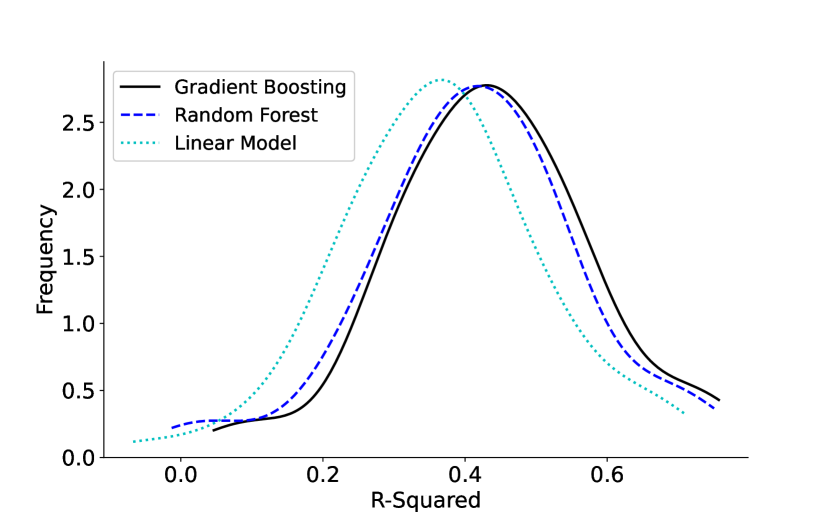
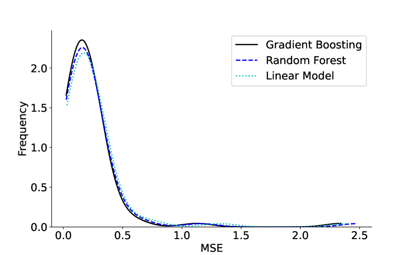
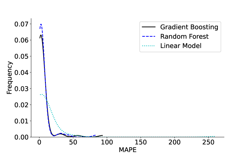
Figure 4: Empirical distributions of the models $\mbox{R}^{2},\mbox{MSE},\mbox{MAPE}$, respectively. Each measure is computed on each hive separately over the test set of the production period.

4.1 Models Explanation

After the modeling process, we now consider the interpretability of the trained tree-based models through an extensive feature importance analysis. All the methodologies applied are again on the models trained over the production period since it is the most interesting from a practical point of view.

Fig. 5 shows the most influential features for the model outcome through an impurity-based feature importances technique that slightly differs depending on the model considered. The importance of a feature, also called Gini importance, is the total reduction of the criterion brought by that feature, where the criterion is the cost function optimized by the method. The squared relative importance of a feature is computed as the sum of the squared improvements on all internal nodes in which it was selected as the splitting variable (Hastie et al., 2009). The higher the mean decrease in impurity over all parallel (RF) or sequential (XGB) trees, the more important the feature is to obtain accurate results. In both cases, the features having greater importance are the lagged versions of the hive weight variation, although lags more distant in the past matter more for XGB predictions. On the contrary, RF attributes the most effective to the previous day’s observation of the hive weight difference. Besides autoregressive components of the input space, the impurity-based measure of past temperature and precipitations lags is effective among the large set of inputs. The average temperature over the past days highly influences the variation in the honey produced in the following 24 hours.

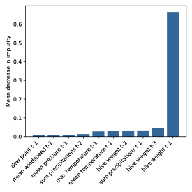
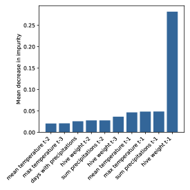
Random Forest	Gradient Boosting

Figure 5: Feature importance for RF (left panel) and XGB (right panel) over the test set in the production period calculated through scikit-learn.

However, a feature importance measure as in Fig. 5 may not be sufficient as it only considers each feature’s contribution to the tree’s purity and not its effect on the model’s predictive capability. The permutation importance technique can be employed to complement the information provided by the mean decrease impurity measure. This method evaluates the importance of each feature by randomly permuting its values and measuring the resulting decrease in the model’s accuracy. A feature is considered important if permuting its values significantly drops the model’s performance. This technique provides a more comprehensive view of feature importance, considering the feature’s effect on the tree structure and its impact on the model’s predictive accuracy. Combining both techniques usually provides a more comprehensive understanding of the relative importance of each feature in the model. Fig. 6 shows the results of this second feature analysis method. The most effective features at improving the model prediction are again past lags of the hive weight variation with temperature and precipitation-based measures that still have an impact. In particular, we notice the greater impact of the previous day’s observation with respect to the other inputs, with the result that does not differ significantly between the two tree-based methods.

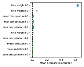
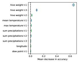
Random Forest	Gradient Boosting

Figure 6: Permutation importance for RF (left panel) and XGB (right panel) over the test set in the production period calculated through scikit-learn.

As a final instrument to shed light on the driver of the predictive capabilities of our machine learning models, we use the SHapley Additive exPlanation (SHAP) framework (see (Lundberg and Lee, 2017; Shapley, 2016)). This approach explains a complex nonlinear model by shedding light on the contribution of each input feature to the output formation. For each input vector $x\in\mathbb{R}^{K}$ and a model $f$, the SHAP value $\varphi_{i}(f,x)$, $i=1,\ldots,K$ quantifies the effect (in a sense, the importance) on the output $f(x)$ of the $i$-th feature. To compute this effect one measures, for any subset $S\subseteq\{1,\ldots,K\}$, the effect of adding/removing the $i$-th feature to the set, i.e. $f_{S\cup\{i\}}(x)-f_{S}(x)$. The SHAP value is defined as the weighted average

$$\varphi_{i}(f,x)=\sum_{S\subseteq\{1,\ldots,K\}\setminus\{i\}}\frac{\left|S\right|!\left(K-\left|S\right|-1\right)!}{K!}\left[f_{S\cup\{i\}}(x)-f_{S}(x)\right],$$ (7)

where the weights ensure that $\sum_{i}\varphi_{i}=f(x)$.

Fig. 7 shows the magnitude of the Shapley values for the test set prediction (production period) of RF and XGB, respectively, on the left and right. The figure helps to understand the relative importance of each feature and its contribution to the model’s output. It displays the features on the y-axis and their importance on the x-axis, quantified by their impact on the model’s output. Features that positively influence the model are placed on the right side of the plot, while those that negatively impact the model are on the left. Each feature is represented by a horizontal bar, colored to indicate the feature’s value for a specific data point according to the color bar placed on the right. The bar height corresponds to the feature’s importance, with the most important features at the top, sorted by importance for quick identification. Even though SHAP values provide a more detailed and nuanced explanation of feature impact with respect to the permutation importance technique, the results are consistent with those in Fig. 5.

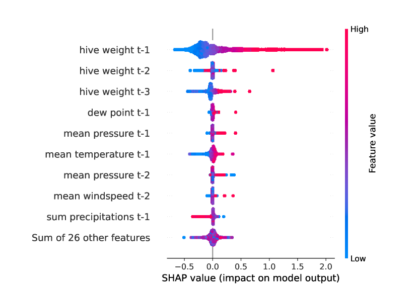
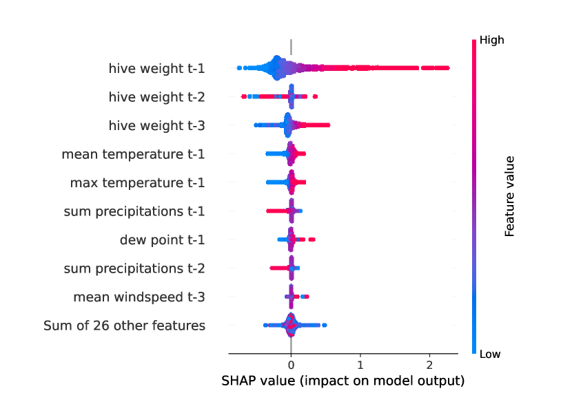
Figure 7: SHAP importance for RF (left panel) and XGB (right panel) over the test set in the production period calculated using the Python package linked to Lundberg and Lee (2017).

5 Conclusions

In this paper, we investigated the use of tree-based methods to predict honey production variation in beehives. We employed both random forest (RF) and extreme gradient boosting (XGB) algorithms. We analyzed the most influential features in the prediction process using impurity-based and permutation-based feature importance techniques, as well as the SHapley Additive exPlanation (SHAP) framework. Our results show that tree-based methods outperform linear models when predicting the hive weight variation using a large set of input features from our dataset. The data covers the period from January 2019 to July 2022 for a total of 431 hives. After extensive data preparation and preprocessing the evidence show that the dynamics of the hive weight variation follow an auto-regressive structure, where the backward-looking lagged values of honey weight variation have a major impact. Among the weather variables, maximum and mean temperature and the total rainfall of the backward-looking lagged values influence more than the others.

Our approach is pioneering in Italy and lays the groundwork for future investigations involving a larger and more comprehensive dataset to fine-tune the models further and improve prediction capability. The increased understanding of the impacts of climatic change could translate into defining weather indicators to pilot best practices for beekeepers and decrease the high risks of production losses which requires urgent measures. Therefore, our findings demonstrate the potential of tree-based methods to predict honey production variation in beehives, with important implications for beekeeping management practices.

Appendix A Feature description

The two tables in this appendix describe the features adopted by the model. Geographical and Seasonality features are not reported since they are fixed factors.

In table 4, we show the features which have been built starting from the daily time series of the variables. For instance, the feature of the hive weight is built by taking the mean of the values in each day.

Feature	Mean	Min	Max	Sum
Hive weight	$\bullet$
Temperature	$\bullet$	$\bullet$	$\bullet$
Precipitations			$\bullet$	$\bullet$
Wind speed	$\bullet$
Radiation	$\bullet$
Pressure	$\bullet$
Dew point	$\bullet$

Table 4: This table reports all the factors built from the daily time series.

In table 5, we report some statistics on the feature time series. In particular, we consider the mean, min, max and standard deviation of all the features. All hives are considered.

Variable	# Features	Mean	Min	Max	Sd
Hive weight	3	0.108	-7.434	7.490	0.664
Temperature	9	0.033	-15.209	6.861	1.418
Precipitations	8	0.001	-8.499	8.521	0.553
Wind speed	3	-0.001	-6.983	6.730	0.756
Radiation	3	0.230	-221.735	257.140	41.898
Pressure	3	0.002	-19.301	26.176	4.051
Dew point	3	0.023	-13.134	9.990	2.218

Table 5: This table shows descriptive statistics of the features. The second column indicates the number of features for each category. The reported values relate to all features created (i.e., the minimum value is the minimum among all features).

Appendix B Hyperparameters of Tree-based Methods

To gain the best possible outcomes from the training process of the tree-based models, we extensively tested the model hyperparameters combination to find the optimal hyperparameters set. The procedure is performed via the stochastic grid search algorithm, performing 2500 iterations with a 5-fold cross-validation method. The optimal model parameters we found are the following:

Random Forest

• N. Trees: 50

• Max Depth: 30

• Ccp Alpha: 0

• Min Samples Split: 200

• Min Samples Leaf: 200

Gradient Boosting

• Eta: 0.08

• Max Depth: 6

• Min Child Weight: 7

References

- (1)
- Alves et al. (2020) Alves, T. S., A., P. M., Ventura, P., Neves, C. J., Biron, D. G., Junior, A. C., De Paula Filho, P. L. and J., R. P. (2020). Automatic detection and classification of honey bee comb cells using deep learning, Computers and Electronics in Agriculture 170: 105244.
- Anwar et al. (2022) Anwar, O., Keating, A., Cardell-Oliver, R., Datta, A. and Putrino, G. (2022). We-bee: Weight estimator for beehives using deep learning, AAAI Conference on Artificial Intelligence 2022: 1st International Workshop on Practical Deep Learning in the Wild.
- Becsi et al. (2021) Becsi, B., Formayer, H. and Brodschneider, R. (2021). A biophysical approach to assess weather impacts on honey bee colony winter mortality, Royal Society open science 8(9): 210618.
- Bhusal and Thapa (2006) Bhusal, S. and Thapa, R. (2006). Response of colony strength to honey production: regression and correlation analysis, Journal of the Institute of Agriculture and Animal Science 27: 133–137.
- Breiman (2001) Breiman, L. (2001). Random forests, Machine Learning 45: 5–32.
- Breiman et al. (1984) Breiman, L., Friedman, J.-H., Olshen, R.-A. and Stone, C.-J. (1984). Classification and regression trees, The Wadsworth Statistics/Probability Series. Belmont, California: Wadsworth International Group, Inc. X, 358.
- Calovi et al. (2021) Calovi, M., Grozinger, C.-M., Miller, D. A. and Goslee, S. C. (2021). Summer weather conditions influence winter survival of honey bees (apis mellifera) in the northeastern united states, Scientific reports 11 1: 1553.
- Campbell et al. (2020) Campbell, T., Dixon, K.-W., Dods, K., Fearns, P. and Handcock, R. (2020). Machine learning regression model for predicting honey harvests, Agriculture 10(4): 1–17.
- Catania and Vallone (2020) Catania, P. and Vallone, M. (2020). Application of a precision apiculture system to monitor honey daily production, Sensors 20(7): 2012.
- Chen and Guestrin (2016) Chen, T. and Guestrin, C. (2016). Xgboost: A scalable tree boosting system, Proceedings of the 22nd ACM SIGKDD International Conference on Knowledge Discovery and Data Mining, KDD ’16, Association for Computing Machinery, New York, NY, USA, p. 785–794.
- Clarke and Robert (2018) Clarke, D. and Robert, D. (2018). Predictive modelling of honey bee foraging activity using local weather conditions, Apidologie 49(3): 386–396.
- Dainat et al. (2012) Dainat, B., Evans, J.-D., Chen, Y.-P., Gauthier, L. and Neumann, P. (2012). Dead or alive: deformed wing virus and varroa destructor reduce the life span of winter honeybees, Applied and environmental microbiology 78(4): 981–987.
- Delaplane et al. (2000) Delaplane, K., Mayer, D. et al. (2000). Crop pollination by bees, CABI publishing.
- Flores et al. (2019) Flores, J., Gil-Lebrero, S., Gámiz, V., M.I., R., Ortiz, M. and Quiles, F. (2019). Effect of the climate change on honey bee colonies in a temperate mediterranean zone assessed through remote hive weight monitoring system in conjunction with exhaustive colonies assessment, Science of The Total Environment 653: 1111–1119.
- Food and Agriculture Organization of the United Nations (2018) (FAO) Food and Agriculture Organization of the United Nations (FAO) (2018). Why bees matter: The importance of bees and other pollinators for food and agriculture.
- Friedman (2001) Friedman, J. H. (2001). Greedy function approximation: a gradient boosting machine, Annals of statistics pp. 1189–1232.
- Garibaldi et al. (2014) Garibaldi, L. A., Carvalheiro, L. G., Leonhardt, S. D., Aizen, M. A., Blaauw, B. R., Isaacs, R., Kuhlmann, M., Kleijn, D., Klein, A. M., Kremen, C. et al. (2014). From research to action: enhancing crop yield through wild pollinators, Frontiers in Ecology and the Environment 12(8): 439–447.
- Gordo and Sanz (2006) Gordo, O. and Sanz, J. (2006). Temporal trends in phenology of the honey bee apis mellifera (l.) and the small white pieris rapae (l.) in the iberian peninsula (1952–2004), Ecological Entomology 31(3): 261–268.
- Gounari et al. (2022) Gounari, S., Proutsos, N. and Goras, G. (2022). How does weather impact on beehive productivity in a mediterranean island?, Italian Journal of Agrometeorology (1): 65–81.
- Gray et al. (2019) Gray, A., Brodschneider, R., Adjlane, N., Ballis, A., Brusbardis, V., Charrière, J.-D., Chlebo, R., Coffey, M. F., Cornelissen, B., da Costa, C. A., Csáki, T., Dahle, B., Danihlík, J., Dražić, M. M., Evans, G., Fedoriak, M., Forsythe, I., de Graaf, D., Gregorc, A., Johannesen, J., Kauko, L., Kristiansen, P., Martikkala, M., Martín-Hernández, R., Medina-Flores, C. A., Mutinelli, F., Patalano, S., Petrov, P., Raudmets, A., Ryzhikov, V. A., Simon-Delso, N., Stevanovic, J., Topolska, G., Uzunov, A., Vejsnaes, F., Williams, A., Zammit-Mangion, M. and Soroker, V. (2019). Loss rates of honey bee colonies during winter 2017/18 in 36 countries participating in the coloss survey, including effects of forage sources, Journal of Apicultural Research 58(4): 479–485.
- Hadjur et al. (2022) Hadjur, H., Ammar, D. and Lefèvre, L. (2022). Toward an intelligent and efficient beehive: A survey of precision beekeeping systems and services, Computers and Electronics in Agriculture 192: 106604.
- Hambleton (1925) Hambleton, J. I. (1925). The Quantitative and Qualitative Effect of Weather Upon Colony Weight Changes, Journal of Economic Entomology 18(3): 447–448.
- Hastie et al. (2009) Hastie, T., Tibshirani, R. and Friedman, J. (2009). The elements of statistical learning: data mining, inference, and prediction, 2. ed edn, Springer, New York, NY, USA.
- Hastono et al. (2017) Hastono, T., Santoso, A. and Pranowo (2017). Honey yield prediction using tsukamoto fuzzy inference system, 2017 4th International Conference on Electrical Engineering, Computer Science and Informatics (EECSI), pp. 1–6.
- Holmes (2002) Holmes, W. (2002). The influence of weather on annual yields of honey, The Journal of Agricultural Science 139(1): 95–102.
- Karaboga and Ozturk (2011) Karaboga, D. and Ozturk, C. (2011). A novel clustering approach: Artificial bee colony (abc) algorithm, Applied soft computing 11(1): 652–657.
- Karadas and Kadirhanoğulları (2017) Karadas, K. and Kadirhanoğulları, I. (2017). Predicting honey production using data mining and artificial neural network algorithms in apiculture, Pakistan Journal of Zoology 49: 1611–1619.
- Klein et al. (2007) Klein, A. M., Vaissière, B. E., Cane, J. H., Steffan-Dewenter, I., Cunningham, S. A., Kremen, C. and Tscharntke, T. (2007). Importance of pollinators in changing landscapes for world crops, Proceedings. Biological sciences 274(1608): 303–313.
- Le Conte and Navajas (2008) Le Conte, Y. and Navajas, M. (2008). Climate change: impact on honey bee populations and diseases, Revue Scientifique et Technique-Office International des Epizooties 27(2): 499–510.
- Lundberg and Lee (2017) Lundberg, S. M. and Lee, S.-I. (2017). A unified approach to interpreting model predictions, Advances in neural information processing systems 30.
- Millennium Ecosystem Assessment (2005) (MEA) Millennium Ecosystem Assessment (MEA) (2005). Ecosystems and Human Well-being: Synthesis, Vol. 5, Island press, Washington, DC, USA.
- Muñoz Sabater et al. (2021) Muñoz Sabater, J., Dutra, E., Agustí-Panareda, A., Albergel, C., Arduini, G., Balsamo, G., Boussetta, S., Choulga, M., Harrigan, S., Hersbach, H., Martens, B., Miralles, D. G., Piles, M., Rodríguez-Fernández, N. J., Zsoter, E., Buontempo, C. and Thépaut, J.-N. (2021). Era5-land: a state-of-the-art global reanalysis dataset for land applications, Earth System Science Data 13(9): 4349–4383.
- Muñoz Sabater (2021) Muñoz Sabater, J. (2021). Era5-land hourly data from 1950 to 1980, Copernicus Climate Change Service (C3S) Climate Data Store (CDS). (Accessed on 23-Sep-2022) .
- Muñoz Sabater et al. (2019) Muñoz Sabater, J. et al. (2019). Era5-land hourly data from 1981 to present, Copernicus Climate Change Service (C3S) Climate Data Store (CDS). (Accessed on 23-Sep-2022) .
- Nasr et al. (2014) Nasr, M. E., Thorp, R., Tyler, T. and Briggs, D. (2014). Estimating Honey Bee (Hymenoptera: Apidae) Colony Strength by a Simple Method: Measuring Cluster Size, Journal of Economic Entomology 83(3): 748–754.
- Ngo et al. (2021) Ngo, T. N., Rustia, D. J. A., Yang, E. and Lin, T. (2021). Automated monitoring and analyses of honey bee pollen foraging behavior using a deep learning-based imaging system, Computers and Electronics in Agriculture 187: 106239.
- Opitz and Maclin (1999) Opitz, D. and Maclin, R. (1999). Popular ensemble methods: An empirical study, Journal of artificial intelligence research 11: 169–198.
- Overturf et al. (2022) Overturf, K., Steinhauer, N., R., M., Wilson, M. E., Watt, A., Cross, R., vanEngelsdorp, R., Williams, G. and S.R., R. (2022). Winter weather predicts honey bee colony loss at the national scale, Ecological Indicators 145: 109709.
- Porrini et al. (2016) Porrini, C., Mutinelli, F., Bortolotti, L., Granato, A., Laurenson, L., Roberts, K., Gallina, A., Silvester, N., Medrzycki, P., Renzi, T., Sgolastra, F. and Lodesani, M. (2016). The status of honey bee health in italy: Results from the nationwide bee monitoring network, PloS one 11(5): e0155411–e0155411.
- Quinlan et al. (2022) Quinlan, G., Sponsler, D., Gaines-Day, H., H.B.G., H. B. M.-S., Otto, C., A.H., S., Colin, T., Gratton, C., R., I., Johnson, R., M.O., M. and Grozinger, C. (2022). Grassy–herbaceous land moderates regional climate effects on honey bee colonies in the northcentral us, Environmental Research Letters 17(6): 064036.
- Rafael Braga, G. Gomes, M. Freitas and A. Cazier (2020) Rafael Braga, A., G. Gomes, D., M. Freitas, B. and A. Cazier, J. (2020). A cluster-classification method for accurate mining of seasonal honey bee patterns, Ecological Informatics 59: 101107.
- Rafael Braga, G. Gomes, Rogers, E. Hassler, M. Freitas and A. Cazier (2020) Rafael Braga, A., G. Gomes, D., Rogers, R., E. Hassler, E., M. Freitas, B. and A. Cazier, J. (2020). A method for mining combined data from in-hive sensors, weather and apiary inspections to forecast the health status of honey bee colonies, Computers and Electronics in Agriculture 169: 105161.
- Shapley (2016) Shapley, L. S. (2016). 17. A value for n-person games, Princeton University Press.
- Solovev (2020) Solovev, V. V. (2020). Influence of weather conditions on the honey productivity of bee colonies in the valdai district of the novgorod region, IOP Conference Series: Earth and Environmental Science 613(1): 12142.
- Switanek et al. (2017) Switanek, M., Crailsheim, K., Truhetz, H. and Brodschneider, R. (2017). Modelling seasonal effects of temperature and precipitation on honey bee winter mortality in a temperate climate, Science of the Total Environment 579: 1581–1587.
- Szabo (1980) Szabo, T. (1980). Effect of weather factors on honeybee flight activity and colony weight gain, Journal of apicultural research 19(3): 164–171.
- Tassinari et al. (2013) Tassinari, W., Lorenzon, M. and Peixoto, E. (2013). Spatial regression methods to evaluate beekeeping production in the state of rio de janeiro, Arquivo Brasileiro de Medicina Veterinária e Zootecnia 65: 553–558.
- Tscharntke et al. (2012) Tscharntke, T., Clough, Y., Wanger, T. C., Jackson, L., Motzke, I., Perfecto, I., Vandermeer, J. and Whitbread, A. (2012). Global food security, biodiversity conservation and the future of agricultural intensification, Biological Conservation 151(1): 53–59. Advancing Environmental Conservation: essays in honor of Navjot Sodhi.
- Yesugade et al. (2018) Yesugade, K., Kharde, A., Mirashi, K., Muley, K. and Chudasama, H. (2018). Machine learning approach for crop selection based on agro-climatic conditions, Machine Learning 7(10).
- Zacepins et al. (2012) Zacepins, A., Stalidzans, E. and Meitalovs, J. (2012). Application of information technologies in precision apiculture, Proceedings of the 13th International Conference on Precision Agriculture (ICPA 2012), Indianapolis, IN, USA.