Optimal Goal-Reaching Reinforcement Learning via Quasimetric Learning

Abstract

In goal-reaching reinforcement learning (RL), the optimal value function has a particular geometry, called quasimetric structure. This paper introduces Quasimetric Reinforcement Learning (QRL), a new RL method that utilizes quasimetric models to learn optimal value functions. Distinct from prior approaches, the QRL objective is specifically designed for quasimetrics, and provides strong theoretical recovery guarantees. Empirically, we conduct thorough analyses on a discretized MountainCar environment, identifying properties of QRL and its advantages over alternatives. On offline and online goal-reaching benchmarks, QRL also demonstrates improved sample efficiency and performance, across both state-based and image-based observations.

Project Page:	tongzhouwang.info/quasimetric_rl
Code:	github.com/quasimetric-learning/quasimetric-rl

1 Introduction

Modern decision-making problems often involve dynamic programming on the cost-to-go function, also known as the value function. This function allows for bootstrapping, where a complicated decision is broken up into a series of subproblems. Once a subproblem is solved, its subgraph can be collapsed into a single node whose cost is summarized by the value function. This approach appears in nearly all contemporary RL and planning algorithms.

In deep RL, value functions are modeled with general neural nets, which are universal function approximators. Further, most RL algorithms focus on optimizing toward a single goal. In this setting, the value function $V^{*}(s)$ reports the (optimal) cost-to-go to achieve that single goal from state $s\in\mathcal{S}$. It is known that $V^{*}$ can be any function $V^{*}\colon\mathcal{S}\rightarrow\mathbb{R}$, that is, for any $V^{*}\colon\mathcal{S}\rightarrow\mathbb{R}$, there exists a Markov Decision Process (MDP) for which that $V^{*}$ is the desired optimal value function.

However, an additional structure emerges when we switch to the multi-task setting, where the (goal-conditioned) value function $V^{*}(s;g)\colon\mathcal{S}\times\mathcal{S}\rightarrow\mathbb{R}$ is the cost-to-go to a given goal state $g$ (Figure 1). In this case, the optimal value function, for any MDP, is always a quasimetric function (Wang & Isola, 2022b; Sontag, 1995; Tian et al., 2020; Liu et al., 2022), which is a generalization of metric functions to allow asymmetry while still respecting the triangle inequality.

Given this structure, it is natural to constrain value function search to the space of quasimetrics. This approach searches within a much smaller subset of the space of all functions $\mathcal{S}\times\mathcal{S}\rightarrow\mathbb{R}$, ensuring that the true value function is guaranteed to be present within this subspace. Recent advancements in differentiable parametric quasimetric models (Wang & Isola, 2022a; Pitis et al., 2020) have already enabled a number of studies (Liu et al., 2022; Wang & Isola, 2022b) to explore the use of these models in standard RL algorithms, resulting in improved performance in some cases.

However, traditional RL algorithms (such as Q-learning (Watkins, 1989)) were designed for large unconstrained function spaces, and their performance may severely degrade with restricted spaces (Wang et al., 2020, 2021). Instead of constraining the search space, they encourage quasimetric properties via the objective function. For example, the Bellman update partly enforces the triangle inequality on the current state, next state, and target goal. With the advent of differentiable parametric quasimetric models, these properties come for free with the architecture, and we aim to design a new RL algorithm specifically geared towards learning quasimetric value functions.

In this work, we propose Quasimetric Reinforcement Learning (QRL). QRL is in the family of geometric approaches to value function learning, which model the value function as some distance metric, or, in our case, a quasimetric. Obtaining local distance estimates is easy because the cost of a single transition is by definition given by the reward function, and can be learned via regression towards observed rewards. However, capturing global relations is hard. This is a problem studied in many fields such as metric learning (Roweis & Saul, 2000; Tenenbaum et al., 2000), contrastive learning (Oord et al., 2018; Wang & Isola, 2020), etc. A general principle is to find a model where local relationships are captured and otherwise states are spread out.

We argue that a similar idea can be used for value function learning. QRL finds a quasimetric value function in which local distances are preserved, but otherwise states are maximally spread out. All three properties are essential in accurately learning the function. Intuitively, a quasimetric function that maximizes the separation of states $s_{0}$ and $s_{1}$, subject to the constraint that it captures cost for each adjacent pair of states, gives exactly the cost of the shortest path from $s_{0}$ to $s_{1}$. It can’t be longer than that due to triangle inequality from quasimetric and preservation of local distances. It can’t be shorter than that due to the maximal spreading. Analogously, consider a chain with several links. If one pushes the chain ends apart, then the distance between the ends is exactly equal to the length of all the links.

These three properties (which we will indicate with the three text colors above) make our method distinct from other contrastive approaches to RL, and ensure that QRL provably learns the optimal value function. Some alternatives use symmetrical metrics that cannot capture complex dynamics (Yang et al., 2020; Ma et al., 2022; Sermanet et al., 2018). Others do not enforce how much adjacent states are pulled together nor how much states are pushed apart, and rely on carefully weighting loss terms and specific sample distributions to estimate on-policy (rather than optimal) values (Eysenbach et al., 2022; Oord et al., 2018).

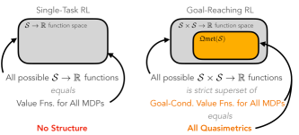
Figure 1: In multi-goal RL, the set of all possible (optimal) value functions is exactly the set of quasimetrics. In single-task RL, there is no similar structure and value functions can be any function.

In summary, our contributions in this paper are

• Based on the connection between value functions and quasimetrics (Section 2), we propose QRL, a new RL framework that utilizes quasimetric models to learn optimal goal-reaching value functions (Section 3).

• We provide theoretical guarantees (Section 3.1) as well as thorough empirical analysis on a discretized MountainCar environment (Section 3.3), highlighting qualitative differences with many existing methods.

• We augment the proposed method to (optionally) also learn optimal Q-functions and/or policies (Section 3.4).

• On offline maze2d tasks, QRL performs well in single-goal and multi-goal evaluations, improving $>37\%$ over the best baseline and $>46\%$ over the d4rl handcoded reference controller (Fu et al., 2020) (Section 5.1).

• Our learned value functions can be directly used in conjunction with trajectory modeling and planning methods, improving their performances (Section 5.1).

• On online goal-reaching settings, QRL shows up to $4.9\times$ improved sample efficiency and performance in both state-based and imaged-based observations, outperforming baselines including Contrastive RL (Eysenbach et al., 2022) and plugging quasimetric Q-function models into existing RL algorithms (Liu et al., 2022) (Section 5.2).

2 Value Functions are Quasimetrics

This section covers the preliminaries on goal-reaching RL settings, value functions, and quasimetrics. We also present a new result showing an equivalence between the latter two.

2.1 Goal-Reaching Reinforcement Learning

We focus on the goal-reaching RL tasks in the form of Markov Decision Processes (MDPs): $(\mathcal{S},\mathcal{A},P,R)$, where $\mathcal{S}$ is the state space, $\mathcal{A}$ is the action space, $P\colon\mathcal{S}\times\mathcal{A}\rightarrow\Delta(\mathcal{S})$ is the transition function, and $R\colon\mathcal{S}\times\mathcal{S}\rightarrow[R_{\mathsf{min}},0]$ is the reward (cost) function for performing a transition between two states. $\Delta(A)$ denotes the set of distributions over set $A$.

Given a target state $s_{\mathsf{goal}}\in\mathcal{S}$, a goal-conditioned agent $\pi(a\mathrel{|}s;s_{\mathsf{goal}})$ is tasked to reach $s_{\mathsf{goal}}$ as soon as possible from the current state $s$. Formally, until the agent reaches the goal, it receives a negative reward (cost) $r(s,s^{\prime})$ for each transition $(s,s^{\prime})$. The agent $\pi$ aims to maximize the expected total reward given any $s$ and $s_{\mathsf{goal}}$, which equals the negated total cost. We call this quantity the (goal-conditioned) on-policy value function $V^{\pi}(s;s_{\mathsf{goal}})$ for $\pi$.

There exists an optimal policy $\pi^{*}$ that is universally optimal:

$$\forall s,s_{\mathsf{goal}},\quad V^{\pi^{*}}(s;s_{\mathsf{goal}})=\max_{\pi}V^{\pi}(s;s_{\mathsf{goal}}).\vspace{-3pt}$$ (1)

We thus define the optimal value function $V^{*}\triangleq V^{\pi^{*}}$.

Similarly, we can define the optimal state-action value function, i.e., Q-function:

$$Q^{*}(s,a;s_{\mathsf{goal}})\triangleq\mathbb{E}_{s^{\prime}\sim P(s,a)}\left[{R(s,s^{\prime})+V^{*}(s^{\prime};s_{\mathsf{goal}})}\right].$$

2.2 Value-Quasimetric Equivalence

Regardless of the underlying MDP, some fundamental properties of optimal value $V^{*}$ always hold.

Triangle Inequality.    As observed in prior works (Wang & Isola, 2022a, b; Liu et al., 2022; Pitis et al., 2020; Durugkar et al., 2021), the optimal value $V^{*}$ always obeys the triangle inequality (due to optimality and Markov property):

$$\forall s_{1},s_{2},s_{3},\quad V^{*}(s_{1};s_{2})+V^{*}(s_{2};s_{3})\leq V^{*}(s_{1};s_{3}).$$ (2)

Intuitively, $V^{*}(s_{1},s_{3})$ is the highest value among all plans from $s_{1}$ to $s_{3}$; and $V^{*}(s_{1};s_{2})+V^{*}(s_{2};s_{3})$ is the highest among all plans from $s_{1}$ to $s_{2}$ and then to $s_{3}$, a more restricted set. Thus, Equation 2 holds, and $-V^{*}$ is just like a metric function on $\mathcal{S}$, except that it may be asymmetrical.

Quasimetrics    are a generalization of metrics in that they do not require symmetry. For a set $\mathcal{X}$, a quasimetric is a function $d\colon\mathcal{X}\times\mathcal{X}\rightarrow\mathbb{R}_{\geq 0}$ such that

$$\forall x_{1},x_{2},x_{3}, \quad d(x_{1},x_{2})+d(x_{2},x_{3})\geq d(x_{1},x_{3})$$ (3)

$$\forall x, \quad d(x,x)=0.$$ (4)

We use $\mathfrak{Qmet}(\mathcal{X})$ to denote all such quasimetrics over $\mathcal{X}$.

Equation 2 shows that $-V^{*}\in\mathfrak{Qmet}(\mathcal{S})$. In fact, the other direction also holds: for any $d\in\mathfrak{Qmet}(\mathcal{S})$, $-d$ is the optimal value function for some MDP defined on $\mathcal{S}$.

Theorem 1 (Value-Quasimetric Equivalence).

$$\mathfrak{Qmet}(\mathcal{S})\equiv\{-V^{*}\colon V^{*} \mathrlap{\text{ is the optimal value of}}$$

$$\hskip 10.00002pt\text{an MDP on $\mathcal{S}$}\}.$$ (5)

Generally, on-policy value $-V^{\pi}$ may not be a quasimetric.

All proofs are deferred to the appendix.

Structure emerges in multi-goal settings.    The space of quasimetrics is the exact function class for goal-reaching RL. In contrast, a specific-goal value function $V^{*}(\,\cdot\,;s_{\mathsf{goal}})$ can be any arbitrary function $\mathcal{S}\rightarrow\mathbb{R}$. In other words, going from single-task RL to multi-task RL may be a harder problem, but also has much more structure to utilize (Figure 1).

2.3 Quasimetric Models and RL

Quasimetric Models refer to parametrized models of quasimetrics $d_{\theta}\in\mathfrak{Qmet}(\mathcal{X})$, where $\theta$ is the parameter to be optimized. Many recent quasimetric models are based on neural networks (Wang & Isola, 2022a, b; Pitis et al., 2020), can be optimized w.r.t. any differentiable objective, and can potentially generalize to unseen inputs (due to neural networks). Many such models can universally approximate any quasimetric and is capable of learning large-scale and complex quasimetric structures (Wang & Isola, 2022a).

An Overview of Quasimetric Models.    A quasimetric model $d_{\theta}$ usually consists of (1) a deep encoder mapping inputs in $\mathcal{X}$ to a generic latent space $\mathbb{R}^{d}$ and (2) a differentiable latent quasimetric head $d_{\mathsf{latent}}\in\mathfrak{Qmet}(\mathbb{R}^{d})$ that computes the quasimetric distance for two input latents. $\theta$ contains both the parameters of the encoder and parameters of the latent head $d_{\mathsf{latent}}$, if any. Recent works have proposed many choices of $d_{\mathsf{latent}}$, which have different properties and performances. We refer interested readers to Wang & Isola (2022a) for an in-depth treatment of such models.

Subtleties of Using Quasimetric Models in RL.    It is tempting to parametrize goal-conditioned value functions with quasimetric models in standard RL algorithms, which optimizes for $V^{*}\in\mathfrak{Qmet}(\mathcal{S})$. However, these algorithms usually use temporal-difference learning or policy iteration, whose success relies on accurate representation of intermediate results (e.g., on-policy values; Theorem 1) (Wang et al., 2020, 2021)) that are not quasimetrics. Indeed, simply using quasimetric models in such algorithms may yield only minor benefits (Wang & Isola, 2022b, a) or require significant relaxations of quasimetric inductive bias (Liu et al., 2022).

Can we directly learn $V^{*}$ without those iterative procedures? Fortunately, the answer is yes, with the help of quasimetrics.

3 Quasimetric Reinforcement Learning

Quasimetric Reinforcement Learning (QRL) at its core learns the optimal goal-conditioned value function $V^{*}$ that is parametrized by a quasimetric model $d_{\theta}\subset\mathfrak{Qmet}(\mathsf{S})$.

Similar to many recent RL works (Kumar et al., 2019; Ghosh et al., 2019; Janner et al., 2022, 2021; Emmons et al., 2021; Chen et al., 2021; Paster et al., 2022; Yang et al., 2022), our method is derived with the assumption that the environment dynamics $P$ are deterministic.

Given ways to sample (e.g., from a dataset / replay buffer)

$$(\overbracket{\vphantom{s^{\prime}}s}^{\mathllap{\textsf{current sta}}\mathrlap{\textsf{te}}},\underbracket{a}_{\mathllap{\textsf{acti}}\mathrlap{\textsf{on}}},\overbracket{s^{\prime}}^{\mathllap{\textsf{ne}}\mathrlap{\textsf{xt state}}},\underbracket{r}_{\mathllap{\textsf{re}}\mathrlap{\textsf{ward}\leq 0}}) \sim p_{\mathsf{transition}}$$ (transitions)

$$s \sim p_{\mathsf{state}}$$ (random state)

$$s_{\mathsf{goal}} \sim p_{\mathsf{goal}},$$ (random goal)

QRL optimizes a quasimetric model $d_{\theta}$ as following:

$$\max_{\theta}~{}\mathbb{E}_{\begin{subarray}{c}s\sim p_{\mathsf{state}}\\ g\sim p_{\mathsf{goal}}\end{subarray}}[d_{\theta}(s,g)]$$ (6)

$$\quad\text{subject to }\mathbb{E}_{\begin{subarray}{c}(s,a,s^{\prime},r)\sim p_{\mathsf{transition}}\end{subarray}}[\mathtt{relu}(d_{\theta}(s,s^{\prime})+r)^{2}]\leq\epsilon^{2},$$

where $\epsilon>0$ is small, and $\mathtt{relu}(x)\triangleq\max(x,0)$ prevents $d_{\theta}(s,s^{\prime})$ from exceeding the transition cost $-r\geq 0$.

After optimization, we take $-d_{\theta}$ as our estimate of $V^{*}$. Section 3.4 discusses extensions that learn optimal Q-functions $Q^{*}$ and policies, making QRL suitable both as a standalone RL method or in conjunction with other RL methods.

3.1 QRL Learns the Optimal Value Function

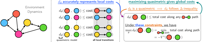
Figure 2: QRL objective finds length of the shortest path connecting two states, i.e., the optimal value $V^{*}$.

By using quasimetric models $d_{\theta}$ to parametrize value functions, we inherently satisfy the triangle-inequality constraints. What additional constraints should we add in order to find the optimal value function for a specific MDP?

A Physical Analogy.   Consider two objects connected by multiple chains. Each chain is formed by several links. If we pull them apart, their distance will be limited by the shortest of all chains. Then, simply measuring the distance between the two objects gives the length of that “optimal” chain. This argument relies on (1) the triangle inequality of our Euclidean physical space and (2) that each link of the chains has a fixed length unaffected by our pulling.

QRL works by the same principles, but in a quasimetric space that both satisfies the triangle inequality and can capture any asymmetrical MDP dynamics (Figure 2):

• Locally, we constrain searching of $V^{*}$ to $d_{\theta}$’s that are consistent with local costs, i.e., not overestimating them:

  $$\mathllap{\forall\ \mathsf{transition}}\ (s,a,s^{\prime},r),\quad d_{\theta}(s,s^{\prime})\mathrlap{{}\leq-r.}$$ (7)

  We ensure this because $d_{\theta}$ should approximate $-V^{*}$ and

  $$-V^{*}(s;s^{\prime})\leq\mathsf{cost\ of\ specific\ path\ }s\xrightarrow{\mathsf{action\ }a}s^{\prime}=-r.$$

• Globally, since $d_{\theta}$ is a quasimetric that satisfies the triangle inequality and Equation 7, for every state $s$ and goal $g$, any path $s\rightarrow g$ places a constraint on $d_{\theta}(s,g)$:

  $$d_{\theta}(s,g)\leq\mathsf{total\ cost\ of\ path\ connecting\ }s\mathsf{\ to\ }g.$$

  Optimal cost from $s$ to $g$ is given by pulling them apart:

  $$\max_{\theta}d_{\theta}(s,g) =\mathsf{cost\ of\ shortest\ path\ connecting\ }s\mathsf{\ to\ }g$$

  $$=-V^{*}(s;g).$$ (8)

Optimal quasimetric $-V^{*}$ achieves this maxima for all $(s,g)$ pairs. Therefore, we maximize $d_{\theta}(s,g)$ simultaneously for all $(s,g)$ pairs:

$$\theta^{*} =\operatorname*{arg\,max}_{\theta}\mathbb{E}_{\begin{subarray}{c}s\sim p_{\mathsf{state}}\\ g\sim p_{\mathsf{goal}}\end{subarray}}[d_{\theta}(s,g)]$$ (9)

$$\qquad\hskip 10.0pt\text{subject to }\forall(s,a,s^{\prime},r)~{}\mathsf{transition},d_{\theta}(s,s^{\prime})\leq-r.$$

This gives exactly the optimal value:

$$d_{\theta^{*}}(s,g)=-V^{*}(s;g),\qquad\forall s,g,$$ (10)

(assuming that $p_{\mathsf{state}}$ and $p_{\mathsf{goal}}$ having sufficient coverage).

The linear programming characterization of $V^{*}$ (Manne, 1960; Denardo, 1970) is similar to Equation 9. However, instead of enforcing triangle inequalities via $\left\lvert\mathcal{A}\right\rvert\left\lvert\mathcal{S}\right\rvert^{2}$ constraints, our quasimetric models automatically satisfy them.

3.1.1 Theoretical Guarantees

We now formally state the recovery guarantees for QRL in both the ideal setting (i.e., optimizing over entire $\mathfrak{Qmet}(\mathcal{S})$) and the function approximation setting.

The proofs of the following results are mostly formalizations of the ideas above. All proofs are presented in Appendix B.

Theorem 2 (Exact Recovery).

If Equation 9 optimizes $d_{\theta}$ over the entire $\mathfrak{Qmet}(\mathcal{S})$, then for $s\sim p_{\mathsf{state}},g\sim p_{\mathsf{goal}}$, we have $d_{\theta^{*}}(s,g)=-V^{*}(s;g)$ almost surely.

In the more realistic case, we use a quasimetric family that is not quite as big as the entire $\mathfrak{Qmet}(\mathcal{S})$ but flexible enough to have universal approximation (e.g., IQE (Wang & Isola, 2022a)). Using a relaxed constraint, we still have a strong guarantee of recovering true $V^{*}$, ensuring a small error even for $(s,g)$ pairs that are far apart.

Theorem 3 (Function Approximation; Informal).

Consider a quasimetric model family $\{d_{\theta}\}_{\theta}$ that is a universal approximator of $\mathfrak{Qmet}(\mathcal{S})$ (in terms of $L_{\infty}$ error). If we solve Equation 9 with a relaxed constraint, where

$$\forall(s,a,s^{\prime},r)~{}\mathsf{transition},\quad\mathtt{relu}(d_{\theta}(s,s^{\prime})+r)\leq\epsilon,$$ (11)

for small $\epsilon>0$. Then, for $s\sim p_{\mathsf{state}},g\sim p_{\mathsf{goal}}$, we have

$$\big{\lvert}{d_{\theta^{*}}(s,g)+(1+\epsilon)V^{*}(s;g)}\big{\rvert}\in[-\sqrt{\epsilon},0],$$

i.e., $d_{\theta^{*}}(s,g)$ recovers $-V^{*}(s;g)$ up to a known scale, with probability $1-\mathcal{O}(-\sqrt{\epsilon}\cdot\mathbb{E}[V^{*}])$.

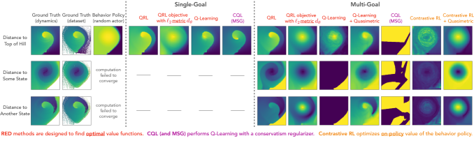
Figure 3: Learned value functions on offline MountainCar. Each plot shows the estimated values from every state towards a single goal (indicated in the leftmost column) as a $2$-dimensional image (velocity as $x$-axis, position as $y$-axis). Left: Ground truth distances, as well as the (expected) distance for the behavior policy that generated training data. Middle: Learned value functions for single-goal methods. Right: Learned value functions for multi-goal methods. Only QRL accurately recovers the ground truth distance structure in both settings, which crucially relies on the asymmetry of quasimetrics. Q-learning methods generally fail in multi-goal settings. Their learned values, while improved with quasimetric models, cannot capture the fine details. Contrastive RL only inaccurately estimates the on-policy values.

3.2 A Practical Implementation

Quasimetric Model.    We use Interval Quasimetric Embeddings (IQE; Wang & Isola (2022a)) as our quasimetric model family $\smash{\{d_{\theta}\}_{\theta}}$. IQEs have convincing empirical results in learning various quasimetric spaces, and enjoy strong approximation guarantees (as needed in Theorem 3).

Constrained Optimization     is done via dual optimization and jointly updating a Lagrange multiplier $\lambda\geq 0$ (Eysenbach et al., 2021). We use a relaxed constraint that local costs are properly modeled in expectation.

Stable Maximization of $d_{\theta}$.    In practice, maximizing $\mathbb{E}[d_{\theta}(s,g)]$ via gradient descent tends to increase the weight norms of the late layers in $d_{\theta}$. This often leads to slow convergence since $\lambda$ needs to constantly catch up. Therefore, we instead place a smaller weight on distances $d_{\theta}(s,g)$ that are already large and optimize $\mathbb{E}[\phi(d_{\theta}(s,g))]$ , where $\phi$ is a monotonically increasing convex function (e.g., affine-transformed softplus). This is similar to the discount factor in Q-learning, which causes its MSE loss to place less weight on transitions of low value.

Full Objective.    Putting everything together, we implement QRL to jointly update $(\theta,\lambda)$ according to

$$\min_{\theta}\max_{\lambda\geq 0}-\mathbb{E}_{\begin{subarray}{c}s\sim p_{\mathsf{state}}\\ g\sim p_{\mathsf{goal}}\end{subarray}}[\phi(d^{\mathsf{IQE}}_{\theta}(s,g))]+{}$$

$$\qquad\lambda\left(\mathbb{E}_{\begin{subarray}{c}(s,a,s^{\prime},r)\sim p_{\mathsf{transition}}\end{subarray}}[\mathtt{relu}(d^{\mathsf{IQE}}_{\theta}(s,s^{\prime})+r)^{2}]-\epsilon^{2}\right).$$ (12)

3.3 Analyses and Comparisons via Discretized MountainCar

We empirically analyze QRL and compare to previous works via experiments on the MountainCar environment with a discretized state space. In this environment, the agent observes the location and velocity of a car, and controls it to reach the top of a hill. Due to gravity and velocity, the dynamics are highly asymmetrical. We discretize the $2$-dimensional state space into $160\times 160$ bins so that we can compute the ground truth value functions. We collected an offline dataset by running a uniform random policy, and evaluated the learning result of various methods, including

• QRL, our method;

• Using QRL objective to train a symmetrical $\ell_{2}$ distance value function;

• Q-Learning with regular unconstrained Q function class;

• Q-Learning with quasimetric function class;

• Contrastive RL (Eysenbach et al., 2022), which uses a contrastive objective but estimates on-policy values;

• Contrastive RL with quasimetric function class;

• Conservative Q-Learning (CQL) (Kumar et al., 2020), which regularizes Q-Learning to reduce over-confidence in out-of-distribution regions;

• Model Standard-deviation Gradients (MSG) (Ghasemipour et al., 2022), a state-of-the-art offline RL algorithm using an ensemble of up to $64$ CQL value functions to estimate uncertainty and train policy;

• Diffuser (Janner et al., 2022), a representative trajectory modelling methods with goal-conditioned sampling.

QRL can be used for both single-goal and multi-goal settings by specifying $p_{\mathsf{goal}}$. For methods that are not designed for multi-goal settings (MSG and Q-Learning), we use Hindsight Experience Replay (HER; Andrychowicz et al. (2017)) to train the goal-conditioned value functions.

Figure 4: Learning dynamics on the offline MountainCar setting. Each plot shows the learned values from every state towards a single goal (indicated at the top) as a $2$-dimensional image (velocity as $x$-axis, position as $y$-axis). Yellow is greater distance (lower value function). Bottom row shows the ground truth distances based on true environment dynamics, and ground truth distances based on transitions appearing in dataset. QRL generally learns the target value function structures much earlier than Q-learning methods.

Evaluation.    Visually, we compare the learned values against ground truths (Figures 4 and 3). We test the agents’ control performances in both reaching the original goal, top of the hill, as well as $9$ distinct states (Section 3.3). A diverse set of goals allows us to evaluate how well the value functions capture the true environment dynamics structure. For QRL and Q-Learning, agents take the action that greedily maximizes the estimated value for simplicity. We describe how to obtain Q-values for QRL later in Section 3.4.

Q-Learning    is the standard way to train optimal value functions for such discrete-action space environments. Despite its popularity, many issues have been identified with its temporal-difference training, such as slow convergence (Lyle et al., 2022; Fujimoto et al., 2022). Figure 4 visualizes the learning dynamics of Q-Learning and QRL, where vanilla Q-Learning indeed learns very slowly. While using a quasimetric Q-function helps significantly, QRL still learns the $V^{*}$ structure much faster, and better captures the true target $V^{*}$ even after training concludes (Figure 3). In planning (Section 3.3), vanilla Q-Learning and (Q-Learning based) MSG struggle in multi-goal settings. While Q-Learning with quasimetrics achieves comparable planning performance with QRL, the higher-quality $V^{*}$ estimate from QRL is likely important in more complex environments. Furthermore, with continuous action spaces, Q-Learning requires a jointly learned actor, which (1) reduces to on-policy value learning and (2) can have complicated training dynamics as the actor’s on-policy values may not be a quasimetric (Theorem 1). QRL is exempt from such issues. In later sections with experiments on online learning in more complex environments, simply using quasimetric in traditional value training indeed greatly underperforms QRL (Section 5.2).

Contrastive RL    uses an arguably similar contrastive objective. However, it samples positive pairs from the same trajectory, and does not enforce exact representation of local costs. Hence, it estimates the on-policy values that generated the data (random actor in this case). Indeed, Figure 3 shows that the Contrastive RL value functions mostly resemble that of a random actor, and fails to capture the boundaries separating states that have distinct values under optimal actors. As shown in Section 3.3, this indeed leads to much worse control results.

Ablations.    We highlight three ablation studies here:

• Asymmetry. QRL objective with symmetrical value functions underperforms QRL greatly, suggesting the importance of asymmetry from quasimetrics.

• Optimality. Contrastive RL with quasimetric can be seen as a method that uses quasimetric to train on-policy values. Thus, the learned values fail to capture optimal decision structures. QRL instead enforces consistency with observed local costs and maximal spreading of states, which leads to optimal values and better performance.

• QRL Objective. While Q-Learning with quasimetrics plans comparably well here , it learns more slowly than QRL (Figure 4) and fails to capture finer value function details (Figure 3). As discussed above, Q-Learning (with or without quasimetrics) also has potential issues with complex dynamics and/or continuous action space, while QRL does not have such problems and attain much superior performance in such settings (see later Section 5.2).

Method	Method Configuration	Task
		Reach Top of Hill	Reach $9$ States
QRL	Single-Goal	97.69 ± 0.26	—
	Multi-Goal	95.89 ± 0.55	85.55 ± 3.57
1-4 Q-Learning	—	98.74 ± 0.19	—
	+ Relabel	89.27 ± 11.69	22.06 ± 8.72
1-4 Contrastive RL	—	83.91 ± 8.04	53.75 ± 32.93
1-4 MSG	—	97.44 ± 0.22	—
	+ Relabel	14.30 ± 0.00	37.80 ± 8.20
1-4 Diffuser	—	19.78 ± 3.03	36.41 ± 1.44
QRL Objective [-0.2ex]with Symmetric $\ell_{2}$ Distance	Single-Goal	95.42 ± 0.16	—
	Multi-Goal	96.13 ± 0.12	73.27 ± 0.84
1-4 Contrastive RL [-0.2ex] + Quasimetric Q-Function	—	83.90 ± 8.73	72.28 ± 4.63
1-4 Q-Learning [-0.2ex] + Quasimetric Q-Function	+ Relabel	96.33 ± 0.37	85.53 ± 3.69
Oracle (Full Dynamics)	—	100.00	100.00
Oracle (Dataset Transitions)	—	69.22	75.89

Table 1: Control results on MountainCar. Scores are normalized returns to reach the desired goal within $200$ steps, averaged across all $160\times 160$ starting states. Each row shows evaluations of a method in a specific configuration with standard deviations from $5$ seeds. We highlight results that are $\geq 95\%$ of the best method.

Compared to existing approaches, QRL efficiently and accurately finds optimal goal-conditioned value functions, showing the importance of both the quasimetric structure and the novel learning objective. In the next section, we describe extensions of QRL, followed by more extensive experiments on offline and online goal-reaching benchmarks in Section 5.

3.4 From $V^{*}$ to $Q^{*}$ and Policy

QRL’s optimal value $V^{*}$ estimate may be used directly in planning to control an agent. A more common approach is to train a policy network w.r.t. to a Q-function estimate (Hafner et al., 2019). This section describes simple extensions to QRL that learn the optimal Q-function $Q^{*}$ and a policy.

Transition and Q-Function Learning.    We augment the quasimetric model $d_{\theta}$ to include an encoder $f\colon\mathcal{S}\rightarrow\mathcal{Z}$:

$$d_{\theta=(\theta_{1},\theta_{2})}(s_{0},s_{1})\triangleq d^{z}_{\theta_{1}}(f_{\theta_{2}}(s_{0}),f_{\theta_{2}}(s_{1})).$$ (13)

Since $d_{\theta}$ captures $V^{*}$, finding the Q-function $Q^{*}(s,a;g)$ only requires knowing the transition result, which we model by a learned latent transition $T\colon\mathcal{Z}\times\mathcal{A}\rightarrow\mathcal{Z}$. In this section, for notation simplicity, we will drop the $()_{\theta_{*}}$ subscript, and use $z\triangleq f(s)$, $z^{\prime}\triangleq f(s^{\prime})$, $\hat{z}^{\prime}\triangleq T(z,a)$, and $z_{g}\triangleq f(g)$.

Once with a well trained $T$, we can estimate $Q^{*}(s,a;g)$ as

$$\smash{d^{z}(\underbracket{T(z,a)}_{\mathllap{\textsf{latent tran}}\mathrlap{\textsf{sition}}},z_{g})\underbracket{\vphantom{T(z,a)}{}-r}_{\mathllap{\textsf{trans}}\mathrlap{\textsf{ition cost}}}=d^{z}(\hat{z}^{\prime},z_{g})-r}\approx-Q^{*}(s,a;g).$$ (14)

(In our experiments, transition cost $-r$ is a constant, and thus omitted. Generally, $T$ can be extended to estimate $r$.)

Transition loss. Given transition $(s,a,s^{\prime})$, we define:

$$\mathcal{L}_{\mathsf{transition}}(s,a,s^{\prime};T,d_{\theta}) \triangleq\frac{1}{2}\big{(}d^{z}(\hat{z}^{\prime},z^{\prime})^{2}+d^{z}(z^{\prime},\hat{z}^{\prime})^{2}\big{)},$$

which is used to optimize both $d_{\theta}$ and $T$ in conjunction with the QRL objective in Equation 12.

$\mathcal{L}_{\mathsf{transition}}$ encourages the predicted next latent $\hat{z}^{\prime}$ to be close to the actual next latent $z^{\prime}$ w.r.t. the learned quasimetric function $d^{z}$. This is empirically superior to a simple regression loss on $\mathcal{Z}$, whose scale is meaningless.

More importantly, the quasimetric properties allow us to directly relate $\mathcal{L}_{\mathsf{transition}}$ values to Q-function error:

Suppose $d^{z}(\hat{z}^{\prime},z^{\prime})^{2}+d^{z}(z^{\prime},\hat{z}^{\prime})^{2}\leq\delta^{2}$, which means

$$d^{z}(\hat{z}^{\prime},z^{\prime})\leq\delta\text{ and }d^{z}(z^{\prime},\hat{z}^{\prime})\leq\delta.$$ (15)

For any goal $g$ with latent $z_{g}$, the triangle inequality implies

$$|{\underbracket{d^{z}(\hat{z}^{\prime},z_{g})}_{\mathllap{\textsf{estimated}}\textsf{ }Q^{*}(s,\mathrlap{a;g)}}-\underbracket{d_{\theta}(s^{\prime},g)}_{\mathllap{\textsf{estima}}\mathrlap{\textsf{ted }V^{*}(s^{\prime};g)}}}|=|d^{z}(\hat{z}^{\prime},z_{g})-d^{z}(z^{\prime},z_{g})| \leq\delta.$$

In other words, if $d_{\theta}$ accurately estimates $V^{*}$, our estimated $Q^{*}(s,a;g)$ has bounded error, for any goal $g$, even though we train with a local objective $\mathcal{L}_{\mathsf{transition}}$. Hence, simply training the transition loss locally ensures that Q-function error is bounded globally, thanks to using quasimetrics.

Based on this argument, our theoretical guarantees for recovering $V^{*}$ (Theorems 2 and 3) can be potentially extended to $Q^{*}$ and thus to optimal policy. We leave this as future work.

Policy Learning.    We train policy $\pi\colon\mathcal{S}\rightarrow\Delta(\mathcal{A})$ to maximize the estimated Q-function (Equation 14):

$$\min_{\pi}\mathbb{E}_{\begin{subarray}{c}s\sim p_{\mathsf{state}}\\ g\sim p_{\mathsf{goal}}\end{subarray}}[d^{z}(T(f(s),a),f(g))].$$ (16)

Additionally, we follow standard RL techniques, training two critic functions and optimizing the policy to maximize rewards from the minimum of them (Fujimoto & Gu, 2021; Eysenbach et al., 2022). In online settings, we also use an adaptive entropy regularizer (Haarnoja et al., 2018).

4 Related Work

Contrastive Approaches to RL.    As discussed in Section 1, our objective bears similarity to those of contrastive approaches. However, we also differ with them in that we rely on (1) quasimetric models, (2) consistency with observed local costs, and (3) maximal spreading of states to learn the optimal value function. Most contrastive methods satisfy none of these properties, and instead pull together states sampled from the same trajectory for capturing on-policy value/information (Eysenbach et al., 2022; Ma et al., 2022; Sermanet et al., 2018; Oord et al., 2018). Yang et al. (2020) ensures exact representation of local cost, but also enforces non-adjacent states to have distance $2$ via a metric function, and thus cannot learn optimal values. Another related line of work trains contrastive models to estimate the alignment between current state and some abstract goal (e.g., text), which are then used as reward for RL training (Fan et al., 2022). Despite the similar goal-reaching setting, their trained model is potentially sensitive to training data, and estimates a density ratio rather than the optimal cost-to-go.

Quasimetric Approaches to RL.    Micheli et al. (2020) consider using quasimetrics for multi-task planning, but does not use models that enforce quasimetric properties. Liu et al. (2022) use quasimetric models to parametrize the Q-function, and shows improved performance with DDPG (Lillicrap et al., 2015) and HER (Andrychowicz et al., 2017) on goal-reaching tasks. These prior works mostly only estimate on-policy value functions, and rely on iterative policy improvements to train policies. Zhang et al. (2020b) use a similar quasimetric definition, but does not use quasimetric models and focuses on hierarchy learning. In contrast, our work utilizes the full quasimetric geometry to directly estimate $V^{*}$ and produce high-quality goal-reaching agents. Additionally, the Wasserstein-1 distance induced by the MDP dynamics is also a quasimetric. Durugkar et al. (2021) utilize its dual form to derive a similar training objective for reward shaping, but essentially employ a different 1-dimensional Euclidean geometry for each goal state and forgo much of the quasimetric structure in $V^{*}$.

Metrics and Abstractions in RL.    Many works explored learning different state-space geometric structures. In particular, bisimulation metric also relates to optimality, but is defined for single tasks where its metric distance bounds the value difference Castro (2020); Ferns & Precup (2014); Zhang et al. (2020a). Generally speaking, any state-space abstraction can be viewed as a form of distance structure, including state embeddings that are related to value functions (Schaul et al., 2015; Bellemare et al., 2019), transition dynamics (Mahadevan & Maggioni, 2007; Lee et al., 2020), factorized dynamics (Fu et al., 2021; Wang et al., 2022), etc. While our method also uses an encoder, our focus is to learn a quasimetric that directly outputs the optimal value $V^{*}$ to reach any goal, rather than bounding it for a single task.

	Environment	QRL	Contrastive RL	MSG (#critic $=64$)	MSG + HER (#critic $=64$)	MPPI with GT Dynamics	MPPI with QRL Value	Diffuser	Diffuser with QRL Value Guidance	Diffuser with Handcoded Controller
Single-Goal	large	191.52 ± 18.28	81.65 ± 43.79	159.30 ± 49.40	59.26 ± 46.70	5.1	19.32 ± 22.97	7.98 ± 1.54	10.08 ± 2.97	128.13 ± 2.59
	medium	163.59 ± 9.70	10.11 ± 0.99	57.00 ± 17.20	75.77 ± 9.02	10.2	58.06 ± 42.79	9.48 ± 2.21	10.71 ± 4.59	127.64 ± 1.47
	umaze	71.72 ± 26.21	95.11 ± 46.23	101.10 ± 26.30	55.64 ± 31.82	33.2	74.85 ± 21.30	44.03 ± 2.25	42.30 ± 3.87	113.91 ± 3.27
	Average	142.27	62.29	105.80	63.56	16.17	50.74	20.50	21.03	123.23
Multi-Goal	large	187.71 ± 7.62	172.64 ± 5.13	—	44.57 ± 25.30	8	37.73 ± 16.67	13.09 ± 1.00	21.26 ± 2.95	146.94 ± 2.50
	medium	150.51 ± 3.77	137.01 ± 6.26	—	99.76 ± 9.83	15.4	56.79 ± 7.66	19.21 ± 3.56	33.39 ± 2.78	119.97 ± 1.22
	umaze	150.60 ± 5.32	142.43 ± 11.99	—	27.90 ± 10.39	41.2	87.49 ± 9.72	56.22 ± 3.90	69.96 ± 2.39	128.53 ± 1.00
	Average	162.94	150.69	—	57.41	21.53	60.67	29.51	41.54	131.81

Table 2: Planning results on maze2d. Scores represent average normalized episode return, where $100$ represents comparable performance with the d4rl reference handcoded controller. Each column show evaluations of the same method configuration. E.g., we train goal-reaching QRL agents and evaluate them in both single-goal and multi-goal settings. We highlight results that are $\geq 95\%$ of the best method. In both evaluations, QRL agents significantly outperform baselines, including MSG + HER with the ground truth reward function, and MPPI with the ground truth environment dynamics. QRL value functions can also be used with planning methods (MPPI) or trajectory sampling methods (Diffuser), and improve their performances. MPPI with GT Dynamics scores are copied from Janner et al. (2022).

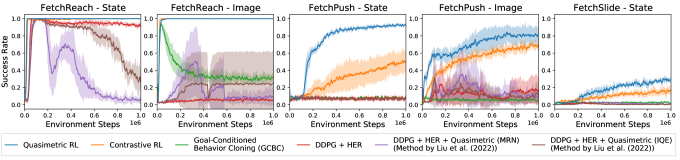
Figure 5: Online learning performance on GCRL benchmarks. No method has access to ground truth reward function. QRL learns faster and better than the baseline methods across all environments for both state-based and image-based observations.

5 Benchmark Experiments

We evaluate QRL learned policies on standard goal-reaching benchmarks in both offline and online settings. All results show means and standard deviations from $5$ seeds. See Appendix C for all experiment details.

5.1 Offline Goal-Reaching d4rl maze2d

Following Diffuser (Janner et al., 2022), we use maze2d environments from d4rl (Fu et al., 2020), and evaluate the learned policies’ performance in (1) reaching the original fixed single goal defined in d4rl as well as (2) reaching goals randomly sampled from the state space. Similar to many offline works (e.g., Contrastive RL (Eysenbach et al., 2022)), we adopt an additional behavior cloning loss for QRL policy optimization in this offline setting.

QRL is a strong method for offline goal-reaching RL.    In Table 2, QRL significantly outperforms all baselines in both single-goal and multi-goal settings. MSG uses a $64$-critic ensemble and is computationally expensive. With only $2$ critics, QRL outperforms MSG by $20\%$ on single-goal tasks and $188\%$ on multi-goal tasks. The Diffuser original paper reported results from a handcoded controller with sampled states as input waypoints. We also report planning using Diffuser’s sampled actions, which attains a much worse result. Regardless, QRL outperforms both Diffuser settings, without using any external information/controller. Compared with Contrastive RL, QRL again sees a big improvement, especially in the single-goal setting. Since the dataset is not generated by agents trying to reach that goal, the on-policy values estimated by Contrastive RL are likely much worse than the optimal values from QRL.

QRL learned value function improves planning and trajectory sampling methods.    Given the high quality of QRL value functions, we can use it to improve other methods. MPPI (Williams et al., 2015) is a model-based planning method. When planning with QRL Q-function, MPPI greatly improves over using ground truth dynamics. We also experiment using QRL Q-function to guide Diffuser’s goal-conditioned sampling, and obtain consistent and non-trivial improvements, especially in multi-goal settings.

5.2 Online Goal-Reaching RL

Following Contrastive RL (Eysenbach et al., 2022) and Metric Residual Networks (MRN; Liu et al. (2022)), we use the Fetch robot environments from the GCRL benchmark (Plappert et al., 2018), where we experiment with both state-based observation as well as image-based observation.

QRL quickly achieves high performance in online RL.    Across all environments, QRL exhibits strong sample-efficiency, and learns the task much faster than the alternatives. Only QRL and Contrastive RL learn in the two more challenging state-based settings, FetchPush and FetchSlide. Compared to Contrastive RL, QRL has $4.9\times$ sample efficiency on state-based FetchPush and $2.7\times$ sample efficiency on state-based FetchSlide. Strictly speaking, image-based observation only contains partial information of the true state, and thus has stochastic dynamics, which violates the assumption of QRL. However, QRL still shows strong performance on image-based settings, suggesting that QRL can potentially also be useful in other partially observable and/or stochastic environments.

QRL outperforms Q-Learning with quasimetric models in complex environments.    Following the approach by Liu et al. (2022), we train standard DDPG (Lillicrap et al., 2015) with relabelling and a quasimetric model Q-function. Essentially, this jointly optimizes a quasimetric Q-function with Q-Learning and a deterministic policy w.r.t. the Q-function. While similar approaches worked well on the simple MountainCar environment (Section 3.3), they fail miserably here on more complex continuous-control settings, as Q-Learning must estimate on-policy Q-function that may not be a quasimetric (Theorem 1). DDPG with quasimetrics are the slowest to learn on state-based FetchReach, and generally are among the least-performing methods. The same pattern holds for two different quasimetric models: IQE and MRN (proposed also by Liu et al. (2022)). In comparison, QRL (which also uses IQE in our implementation) quickly learns the tasks. QRL is more general and scales far better than simply using Q-Learning with quasimetrics.

6 Implications

In this work, we introduce a novel RL algorithm, QRL, that utilizes the equivalence between optimal value functions and quasimetrics. In contrast to most RL algorithms that optimize generic function classes, QRL is designed for using quasimetric models to parametrize value functions. Combining quasimetric models with an objective that captures local distances and maximally spreads out states (Section 3.1), QRL provably recovers the optimal value function (Section 3.1.1) without temporal-difference or policy iteration, making it distinct from many prior approaches.

From thorough analyses on MountainCar, we empirically confirm the importance of different components in QRL, and observe that QRL can learn value functions faster and better than alternatives (Section 3.3). Our experiments on additional benchmarks echo these findings, showing better control results in both online and offline settings (Section 5). QRL can also be used to directly improve other RL methods, and demonstrates strong sample efficiency in online settings.

These QRL results highlight the usefulness of quasimetrics in RL, as well as the benefit of incorporating quasimetric structures into designing RL algorithms.

Below we summarize several exciting future directions.

QRL as Representation and World Model Learning.    QRL can be also viewed as learning a decision-aware representation (via encoder $f$) and a latent world model (via latent dynamics $T$). In this work, for fair comparison, we did not utilize such properties much. However, combining QRL with techniques from these areas (e.g., estimating multi-step return, auxiliary loss training) may yield even stronger performances and/or more general QRL variants (e.g., better support for partial observability and stochasticity).

Quasimetric Structures in Searching and Exploration.    QRL results show that quasimetrics can flexibly model distinct environments and greatly boost sample efficiency. Such learned (asymmetrical) state-space distances potentially have further uses in long-range planning and exploration. A locally distance-preserving quasimetric is always a consistent and admissible heuristic (Pearl, 1984), which guarantees optimality in search algorithms like A* (Hart et al., 1968). Perhaps such exploration ideas may be incorporated in a quasimetric-aware actor, or even for solvers of general searching and planning problems.

Better Exploration for Structure Learning.    In our and most RL works, online exploration is done via noisy actions from the learned policy. Arguably, if an agent is learning the structure of the environment, it should instead smartly and actively probe the environment to improve its current estimate. Consider QRL as an example. If current quasimetric estimate $d_{\theta}(s_{0},s_{1})$ is small but no short path connecting $s_{0}$ to $s_{1}$ was observed, the agent should test if they are actually close w.r.t. the dynamics. Additionally, one may use uncertainty/errors in learned quasimetric distances/dynamics to derive new intrinsic exploration methods. Such advanced exploration may speed up learning the geometric structures of the world, and thus better generalist agents.

More Quasimetric-Aware RL Algorithms.    To our best knowledge, QRL is the first RL method designed for quasimetric models. We hope the strong performance of QRL can inspire more work on RL algorithms that are aware of quasimetric and/or other geometric structures in RL.

Acknowledgements

TW’s contribution in this material is based on work that is partially funded by Google. TW was supported in part by ONR MURI grant N00014-22-1-2740.

Appendix A Discussions and Generalizations of QRL

Self-Transitions    are in fact already handled by the QRL objective presented in this paper (Equations 6 and 12). For any state $s$ (with or without self-transition), we have $V^{*}(s;s)=0$, since the optimal cost to first reach $s$ start from $s$ is given by the empty trajectory. This is naturally enforced by our value function model $-d_{\theta}$, since it is enforced to be a quasimetric. For self-transitions $(s,a,s,r)$ in the training data (where $r\leq 0$ is the reward), their contribution to the constraint loss term will always be $\mathtt{relu}(d_{\theta}(s,s)+r)^{2}=\mathtt{relu}(0+r)^{2}=\mathtt{relu}(r)^{2}=0^{2}=0$. Therefore, the constraints are inherently satisfied for self-transitions. So our theoretical results from Section 3.1.1 also hold for such cases.

Constant Costs.    In many cases (and most goal-reaching benchmarks), each environment transition has a fixed constant cost $C$. In other words, the task is to reach the given goal as quickly as possible. Then, in the QRL constrained optimization, we can drop the $\mathtt{relu}(\cdot)$ and essentially, since we know that $-V^{*}(s;s^{\prime})=C$ for sure, and thus we should have $d_{\theta}(s,s^{\prime})=C$. Technically speaking, the $\mathtt{relu}(\cdot)$ formulation should be able to find the same solution. In our experience, even when it is known that the transition cost is constant, adding this information in the objective, i.e., removing $\mathtt{relu}(\cdot)$, does not significantly change the results.

General Goals (Sets of States).    We can easily extend QRL to general goals, which are sets of states. Let $G\subset\mathcal{S}$ be such a general goal. We augment our models to operate not just on $\mathcal{S}$, but on $\mathcal{S}\bigcup\{G\}$ (which can be simply achieved by, e.g., adding an indicator dimension). When we encounter transition that ends within some $s^{\prime}\in G$, we simultaneously add a transition $(s^{\prime},G)$ to the dataset.

Appendix B Proofs

B.1 Theorem 1: (Value-Quasimetric Equivalence).

Proof of Theorem 1.

We have shown already $-V^{*}\in\mathfrak{Qmet}(\mathcal{S})$. (See also Proposition A.4 of Wang & Isola (2022b).)

For any $d\in\mathfrak{Qmet}(\mathcal{S})$, define

$$\mathcal{A} \triangleq\mathcal{S}$$

$$P(s,s_{\mathsf{act}}) \triangleq\delta_{s_{\mathsf{act}}} \delta_{x} x$$ ( is the Dirac measure at )

$$R(s,s^{\prime}) \triangleq-d(s,s^{\prime}).$$

Then the optimal value of $(\mathcal{S},\mathcal{A},P,R)$ is $-d$, regardless of discounting factor (if any).

For the on-policy values, consider action space $\mathcal{A}=\{a_{\mathsf{self}},a_{\mathsf{next}}\}$. Assume that state-space $\left\lvert\mathcal{S}\right\rvert>2$. Let $s_{1}$, $s_{2}$, $s_{3}$ be three distinct states in $\mathcal{S}$, all transitions have reward $-1$, and

$$P(s_{1},a_{\mathsf{self}}) =\delta_{s_{1}}$$

$$P(s_{2},a_{\mathsf{self}}) =\delta_{s_{2}}$$

$$P(s_{3},a_{\mathsf{self}}) =\delta_{s_{3}} a_{\mathsf{self}}$$ ( is always a self-transition)

$$P(s_{1},a_{\mathsf{next}}) =\delta_{s_{2}}$$

$$P(s_{2},a_{\mathsf{next}}) =\delta_{s_{3}}$$

$$P(s_{3},a_{\mathsf{next}}) =\delta_{s_{1}} a_{\mathsf{next}}$$ ( goes to the next state cyclically)

$$\pi(s_{1};s_{2}) =\delta_{a_{\mathsf{next}}} \pi a_{\mathsf{next}} s_{2} s_{1}$$ ( always takes when tasked to go to from )

$$\pi(s_{2};s_{3}) =\delta_{a_{\mathsf{next}}}$$

$$\pi(s_{1};s_{2}) =\delta_{a_{\mathsf{self}}}.$$

So

$$-V^{\pi}(s_{1};s_{2})=-V^{\pi}(s_{2};s_{3}) =1$$

$$-V^{\pi}(s_{3};s_{1}) =\infty,$$

violating triangle-inequality. ∎

B.2 Theorem 2: (Exact Recovery).

Proof of Theorem 2.

Since the transition dynamics is deterministic, we can say that states $s_{0}$ is locally connected to state $s_{1}$ if $\exists a\in\mathcal{A}$ such that $P(s_{1}\mathrel{|}s_{0},a)=1$. We say a path $(s^{\mathsf{path}}_{0},s^{\mathsf{path}}_{1},s^{\mathsf{path}}_{2},\dots,s^{\mathsf{path}}_{T})$ connects $s_{0}$ to $s_{1}$ if

$$s^{\mathsf{path}}_{0} =s_{0}$$

$$s^{\mathsf{path}}_{i} \text{ is locally connected to }s^{\mathsf{path}}_{i+1},\quad\forall i\in\{0,1,\dots,T-1\}$$

$$s^{\mathsf{path}}_{T} =s_{1}.$$

And we say the total cost of this path is the total rewards over all $T-1$ transitions, i.e., $T-1$.

From the definition of $V^{*}$ and Theorem 1, We know that,

$$-V^{*} \in\mathfrak{Qmet}(\mathcal{S})$$

$$-V^{*}(s;g) =\textsf{total cost of shortest path connecting $s$ to $g$},\qquad\forall s,g.$$

Therefore, the constraints stated in Equation 9 is feasible. The rest of this proof focuses only on $d_{\theta}$’s that satisfy the constraints, which includes $-V^{*}$.

Due to triangle inequality, we have $\forall s,g$,

$$d_{\theta}(s,g)\leq\textsf{total cost of shortest path connecting $s$ to $g$}=-V^{*}(s;g).$$ (17)

Therefore,

$$\mathbb{E}_{s,g}[d_{\theta}(s,g)]\leq\mathbb{E}_{s,g}[-V^{*}(s;g)],$$ (18)

with equality iff $d_{\theta}(s,g)=-V^{*}(s;g)$ almost surely.

Hence, $d_{\theta^{*}}(s,g)=-V^{*}(s;g)$ almost surely.

∎

B.3 Theorem 3: Function Approximation

We first state the more general and formal version of Theorem 3.

Theorem 4 (Function Approximation; General; Formal).

Assume that $\mathcal{S}$ is compact and $V^{*}$ is continuous.

Consider a quasimetric model family that is a universal approximator of $\mathfrak{Qmet}(\mathcal{S})$ in terms of $L_{\infty}$ error (e.g., IQE (Wang & Isola, 2022a) and MRN (Liu et al., 2022)). Concretely, this means that $\forall\epsilon>0$, we can have $\{d^{(\epsilon)}_{\theta}\}_{\theta}$ such that, there exists some $\theta$ where

$$\forall s_{0},s_{1}\in\mathcal{S},\quad\left\lvert d^{(\epsilon)}_{\theta}(s_{0},s_{1})+V(s_{0};s_{1})\right\rvert\leq\epsilon.$$ (19)

Now for some small $\epsilon>0$, consider solving Equation 9 over $\{d^{(\epsilon/2)}_{\theta}\}_{\theta}$ with the relaxed constraint that

$$\forall(s,a,s^{\prime},r)~{}\mathsf{transition},\quad\mathtt{relu}({d^{(\epsilon/2)}_{\theta}(s,s^{\prime})+r})\leq\epsilon,$$ (20)

then for $s\sim p_{\mathsf{state}},g\sim p_{\mathsf{goal}}$, and for all $\delta>0$, we have

$$\left\lvert d_{\theta^{*}}(s,g)+(1+\epsilon)V^{*}(s;g)\right\rvert\in[-\delta,0],$$

with probability $1-\mathcal{O}\left(\frac{\epsilon}{\delta}\cdot(-\mathbb{E}[V^{*}])\right)$.

As a special case with $\delta=\sqrt{\epsilon}$, we have

$$\mathbb{P}\bigg{[}\big{\lvert}{d_{\theta^{*}}(s,g)+(1+\epsilon)V^{*}(s;g)}\big{\rvert}\in[-\sqrt{\epsilon},0]\bigg{]}=1-\mathcal{O}\left(-\sqrt{\epsilon}\cdot\mathbb{E}[V^{*}]\right),$$ (21)

which is exactly Theorem 3.

Note that the compactness and continuity assumptions ensure that $V^{*}$ is bounded. We start by proving a lemma.

Lemma 1.

With the assumptions of Theorem 4, there exists a $d^{(\epsilon/2)}_{\theta^{\dagger}}$ that satisfies the constraint with

$$\mathllap{\forall s,g,\quad}d^{(\epsilon/2)}_{\theta^{\dagger}}(s,g)\geq-V^{*}(s;g).$$ (22)

Proof of Lemma 1.

Let the underlying MDP of $V^{*}$ be $\mathcal{M}=(\mathcal{S},\mathcal{A},P,R)$. Consider another MDP $\tilde{\mathcal{M}}=(\mathcal{S},\mathcal{A},P,R-\frac{\epsilon}{2})$, with optimal goal-reaching value function $\tilde{V}^{*}\in\mathfrak{Qmet}(\mathcal{S})$.

Obviously, transitions $(s,a,s^{\prime},r)$ in $\mathcal{M}$ bijectively correspond to transitions $(s,a,s^{\prime},r-\frac{\epsilon}{2})$ in $\tilde{\mathcal{M}}$.

For any $s$ and $g$, let $s\rightarrow s_{1}\rightarrow s_{2}\rightarrow\dots\rightarrow s_{n-1}\rightarrow g$ be the shortest path connecting $s$ to $g$ in $\tilde{\mathcal{M}}$ via $n$ transitions.

$$-\tilde{V}^{*}(s;g) ={\textsf{total cost of $s\rightarrow s_{1}\rightarrow s_{2}\rightarrow\dots\rightarrow s_{n-1}\rightarrow g$ according to $R-\frac{\epsilon}{2}$ as reward}}$$ (23)

$$=\frac{n\cdot\epsilon}{2}+{\textsf{total cost of $s\rightarrow s_{1}\rightarrow s_{2}\rightarrow\dots\rightarrow s_{n-1}\rightarrow g$ according to $R$ as reward}}$$ (24)

$$\geq\frac{n\cdot\epsilon}{2}+{\textsf{total cost of shortest path connecting $s$ to $g$ in $\mathcal{M}$ according to $R$ as reward}}$$ (25)

$$=\frac{n\cdot\epsilon}{2}-V^{*}(s;g).$$ (26)

Since $n>0$ iff $s\neq g$, we have

$$-\tilde{V}^{*}(s;g)\geq\frac{\epsilon}{2}\cdot\mathbbm{1}_{s\neq g}-V^{*}(s;g),\qquad\forall s,g.$$ (27)

By universal approximation, there exists $d^{(\epsilon/2)}_{\theta^{\dagger}}$ such that

$$\forall s,g,\quad\left\lvert d^{(\epsilon/2)}_{\theta^{\dagger}}(s,g)+\tilde{V}^{*}(s;g)\right\rvert\leq\frac{\epsilon}{2}.$$ (28)

In particular,

• for $s\neq g$, by Equations 27 and 28, we have

  $$d^{(\epsilon/2)}_{\theta^{\dagger}}(s,g)\geq-\tilde{V}^{*}(s;g)-\frac{\epsilon}{2}\geq-V^{*}(s;g);$$ (29)

• for $s=g$, by Equation 28, we have

  $$d^{(\epsilon/2)}_{\theta^{\dagger}}(s,g)=d^{(\epsilon/2)}_{\theta^{\dagger}}(s,s)=0=-V^{*}(s;s)=-V^{*}(s;g).$$ (30)

Hence, $d^{(\epsilon/2)}_{\theta^{\dagger}}\geq-V^{*}$ globally. Now it only remains to show that $d^{(\epsilon/2)}_{\theta^{\dagger}}$ satisfies the constraint.

For any transition $(s,a,s^{\prime},r=R(s,s^{\prime}))$ in $\mathcal{M}$, by Equation 28,

$$d^{(\epsilon/2)}_{\theta^{\dagger}}(s,s^{\prime}) \leq-\tilde{V}^{*}(s;s^{\prime})+\frac{\epsilon}{2}$$ (31)

$$\leq\frac{\epsilon}{2}-R(s,s^{\prime})+\frac{\epsilon}{2} s\rightarrow s^{\prime} \tilde{\mathcal{M}} \frac{\epsilon}{2}-R(s,s^{\prime})$$ (since is also a valid path in with cost )

$$=-r+\epsilon,$$ (32)

which means that $d^{(\epsilon/2)}_{\theta^{\dagger}}$ satisfies the constraint.

Hence the desired $d^{(\epsilon/2)}_{\theta^{\dagger}}$ exists.

∎

Now we are ready to prove Theorems 3 and 4.

Proof of Theorems 3 and 4.

Let $d^{(\epsilon/2)}_{\theta^{*}}$ be the solution to the relaxed problem. By the definition of the universal approximator, such solutions exist. Moreover, we have

$$\forall s,g,\quad d^{(\epsilon/2)}_{\theta^{*}}(s,g)\leq-(1+\epsilon)V^{*}(s;g),$$ (33)

by the constraint and triangle inequality.

Define

$$p\triangleq\mathbb{P}[d^{(\epsilon/2)}_{\theta^{*}}(s,g)<-(1+\epsilon)V^{*}(s;g)-\delta].$$ (34)

Then

$$\mathbb{E}[d^{(\epsilon/2)}_{\theta^{*}}(s,g)]\leq-(1+\epsilon)\mathbb{E}[V^{*}(s;g)]-p\delta,$$ (35)

where we used Equations 33 and 34.

Let $d^{(\epsilon/2)}_{\theta^{\dagger}}$ be the quasimetric from Lemma 1. Then, by optimality, we must have

$$\mathbb{E}[d^{(\epsilon/2)}_{\theta^{*}}(s,g)]\geq\mathbb{E}[d^{(\epsilon/2)}_{\theta^{\dagger}}(s,g)]\geq-\mathbb{E}[V^{*}(s;g)].$$ (36)

Combining Equations 35 and 36, we have

$$-(1+\epsilon)\mathbb{E}[V^{*}(s;g)]-p\delta\geq-\mathbb{E}[V^{*}(s;g)].$$ (37)

Rearranging the terms, we have

$$p \leq\frac{\epsilon}{\delta}\cdot(-\mathbb{E}[V^{*}]).$$ (38)

Combining Equations 38 and 33 gives the desired result. ∎

Appendix C Experiment Details and Additional Results

All our results are aggregation from $5$ runs with different seeds.

We first discuss general design details that holds across all settings. For task-specific details, we discuss them in separate subsections below.

QRL.    Across all experiments, we use $\epsilon=0.25$, initialize Lagrange multiplier $\lambda=0.01$, and use Adam (Kingma & Ba, 2014) to optimize all parameters. $\lambda$ is optimized via a softplus transform to ensure non-negativity. Our latent transition model $T$ is implemented in a residual manner, where

$$T(z,a)\triangleq g_{\phi}(z,a)+z,$$ (39)

and $g_{\phi}$ being a generic MLP with weights and biases of the last fully-connected layer initialized to all zeros. Unless otherwise noted, all networks are implemented as simple ReLU MLPs. $p_{\mathsf{state}}$ is taken to be the beginning state of a random transition sampled from dataset / replay buffer. Unless otherwise noted, $p_{\mathsf{goal}}$ is taken to be the resulting state of a random transition sampled from dataset / replay buffer. For maximizing $d_{\theta}$, unless otherwise noted, we use the strictly monotonically increasing convex function

$$\phi(x)\triangleq-\mathrm{softplus}(500-x,\beta=0.01)=-100\times\mathrm{softplus}(5-\frac{x}{100}).$$ (40)

MSG.    We follow the authors’suggestions, use $64$-critics, and tune the two regularizer hyperparameters over $\alpha\in\{0,0.1,0.5,1\}$ and $\beta\in\{-4,-8\}$. For other hyperparameters, we use the same default values used in the original paper (Ghasemipour et al., 2022).

C.1 Discretized MountainCar

Discretization.    MountainCar state is parametrized by $\textsf{position}\in[-1.2,0.6]$ and $\textsf{velocity}\in[-0.07,0.07]$. For a dimension with values in interval $[l,u]$, we consider $160$ evenly spaced bins of length $(u-l)/159$, with centers being

$$\left\{l+\frac{u-l}{159}\times k\colon k=0,1,2,\dots,159\right\}.$$ (41)

After each reset and transition, we discretize each dimension of the state vector, so that future dynamics start from the discretized vector. To discretize a value, we find the bin it falls into, and replace it with the value of bin center. Note that the two bins at the two ends are centered at $u$ and $l$, respectively. So the two ends are exactly represented. Discretizing each dimension this way leads to $160\times 160$ discrete states.

Data.    In MountainCar, the original environment goal (top of hill) is a set of states with $\textsf{position}\in[0.5,0.6]$ and $\textsf{velocity}\in[0,0.07]$, where the agent is considered reaching that goal if it reaches any of those states. We adapt QRL and other goal-reaching methods to support this general goal following the procedure outlined in Appendix A. Specifically, we augment the observation space to include an additional indicator dimension, which is $1$ only when representing this general goal. In summary, any original (discretized) state $s\triangleq[u,v]$ becomes $\tilde{s}\triangleq[u,v,0]$, and $G\triangleq[0.5,0,1]$ refers to this general goal. All critics and policies now takes in this augmented $3$-dimensional vector as input. For each encountered state $\tilde{s}$ that falls in this set, a new transition $(\tilde{s},G)$ is added to the offline dataset. The dataset includes $240$ such added transitions and $199{,}888$ transitions generated by running a random actor for $1{,}019$ episodes, where each episode terminate when the agent reaches top of hill or times out at $250$ timesteps.

Evaluation.    For each target goal, we evaluate the planning performance starting from each of $160\times 160$ states, with a budget of $200$ steps. At each step, the agent receives $-1$ reward until it reaches the goal. The episode return is then averaged over $160\times 160$ states to compute the statistics. For the task of planning towards $9$ specific states, we say that agent reaches the goal if it reaches a $13\times 13$ neighborhood centered around the goal state, and average the metrics over $9$ target goal states. For QRL and Q-Learning, we did not train any policy network. Instead, the agents take the action that maximizes Q value (or minimizes distance) for simplicity.

Goal Distribution.    For all multi-goal methods, wherever possible, we adopt a goal-sampling distribution as following: for $s_{\mathsf{goal}}\sim p_{\mathsf{goal}}$,

$$s_{\mathsf{goal}}=\begin{cases}\textsf{resulting state from a random transition}&\text{ with probability $0.95$}\\ [0.5,0,1]&\text{ with probability $0.05$}.\end{cases}$$ (42)

QRL.    We use 3-1024-1024-1024-256 network for $f$ and (256+3)-1024-1024-1024-256 residual network for $T$, where $3$ represents the one-hot encoding of $3$ discrete actions. For $d_{\theta}$, we use a 256-1024-1024-1024-256 projector followed by an IQE-maxmean head with $16$ components, each of size $32$. $\mathcal{L}_{\mathsf{transition}}$ is optimized with a weight of $75$. Our learning rate is $0.3$ for $\lambda$ and $5\times 10^{-4}$ for the model parameters. We use a batch size of $4096$ to train $5\times 10^{5}$ gradient steps. For all parameters except $\lambda$, we used cosine learning rate scheduling without restarting, decaying to $0$ at the end of training.

Q-Learning.    We use $x$-1024-1024-1024-1024-1024-1024-3 networks for vanilla Q-Learning, where $x=3$ in the single-goal setting, and $x=6$ in the multi-goal setting. The $3$ outputs represents estimated Q values for all $3$ actions.

Q-Learning with Quasimetrics.     We use the same encoder and projector architecture as QRL, as well as the same IQE specification. Additionally, to model the Q-function, we also add a 256-1024-1024-1024-(3$\times$256) transition model (which outputs the residual for each of the $3$ actions), and adopt QRL’s transition loss with a weight of $5$. In other words, we replace the QRL’s value learning objective with the Q-Learning temporal-difference objective (and keep the transition loss). We use a discount factor of $0.95$, and update the target Q model every $2$ iterations with a exponential moving average factor of $0.005$. We use a learning rate of $0.001$ and a batch size of $4096$ to train $5\times 10^{5}$ gradient steps.

Contrastive RL.    We mostly follow the author’s parameters for their offline experiments, using $x$-1024-1024-1024-$d_{z}$ encoders, where $x=(3+3)$ for the state-action encoder, $x=3$ for the goal encoder, and $d_{z}$ is the latent dimension. We tune $d_{z}\in\{16,64\}$ and choose $64$ for better performance. The policy training is modified to compute exactly the expected Q-value (rather than using a reparametrized sample) from the policy’s output action distribution, to accommodate the discrete action space. Since the dataset is generated from a random actor policy, we disable the behavior cloning loss. We train over $10^{5}$ gradient steps using a batch size of $1024$. We note that Contrastive RL requires a specific goal-sampling distribution, which we use instead of $p_{\mathsf{goal}}$ from Equation 42.

Contrastive RL with Quasimetrics.    We use the same encoder and projector architecture as QRL, as well as the same IQE specification. Similar to Q-Learning, we also add a residual transition model, which uses the same (256+3)-1024-1024-256 architecture as QRL’s transition model, and adopt QRL’s transition loss with a weight of $5$. In other words, we replace the QRL’s value learning objective with the contrastive objective from Contrastive RL (and keep the transition loss). Contrastive RL objective estimates the on-policy Q-function with an extra goal-specific term determined by $p_{\mathsf{goal}}$ (Eysenbach et al., 2022). Thus, we also learn a 256-1024-1024-1 model $c(z_{g})$, where $z_{g}$ is the latent of goal $g$. Contrastive RL loss is computed with the sum of $c(z_{g})$ and quasimetric output. Other hyperparameters are identical to the vanilla Contrastive RL choices.

MSG.    We follow the original paper and tune $\alpha\in\{0,0.1,0.5,1\}$ and $\beta\in\{-4,-8\}$. After tuning, we select $\alpha=0.1$, $\beta=-4$ for both the single-goal and multi-goal setting. For relabelling, we find using random goals hurting performance. Hence, instead of $p_{\mathsf{goal}}$ from Equation 42, we use $[0.5,0.5,1]$ with probability $0.05$, and a future state from the same trajectory with probability $0.95$, where the future state is taken to be $\Delta t\geq 1$ steps away, where $\Delta t\sim\mathrm{Geometric}(0.3)$.

Diffuser.    Diffuser’s training horizon defines the length of trajectory segment used in training. Any trajectory with length shorter than this number won’t be sampled at all for training. We tune the training horizon between $16$ (which includes almost all training trajectories) and $200$ (which excludes shorter trajectories from training but may better capture long-term dependencies), and choose $16$ due to its better performance in both evaluations.

C.2 Offline d4rl maze2d

Evaluation.    For each method, we evaluate both single-goal and multi-goal planning over $100$ episodes.

QRL.    We use 4-1024-1024-1024-256 network for $f$ and (256+2)-1024-1024-1024-256 residual network for $T$, where $2$ is the action dimension. For $d_{\theta}$, we use a 256-1024-1024-2048 projector followed by an IQE-maxmean head with $64$ components, each of size $32$. $\mathcal{L}_{\mathsf{transition}}$ is optimized with a weight of $1$. Our learning rate is $0.01$ for $\lambda$, $5\times 10^{-4}$ for the critic parameters, and $3\times 10^{-5}$ for the policy parameters. We use a batch size of $4096$ to train $2\times 10^{5}$ gradient steps. Inspired by Contrastive RL (Eysenbach et al., 2022), we augment policy training with an additional behavior cloning loss of weight $0.05$ (towards a goal that is $\Delta t\geq 1$ steps in the future from the same trajectory, for $\Delta t\sim\mathrm{Geometric}(0.99)$).

Contrastive RL.    We mostly follow the author’s parameters for their offline experiments, using $x$-1024-1024-1024-16 encoders, where $x=(4+2)$ for the state-action encoder, and $x=4$ for the goal encoder, and $d_{z}$ is the latent dimension, as well as a behavior cloning loss of weight $0.05$. We train over $1.5\times 10^{5}$ gradient steps using a batch size of $1024$. We note that Contrastive RL requires a specific goal-sampling distribution, which we use instead of $p_{\mathsf{goal}}$ from Equation 42.

MSG.    For single-goal results, we report the evaluations from the original paper. For multi-goal tasks, we use the same architectures with relabelling, and tune $\alpha\in\{0,0.1,0.5,1\}$ and $\beta\in\{-4,-8\}$, following the procedure from original paper. After tuning, we use $\alpha=0.1$ and $\beta=-8$ for the large maze, $\alpha=0.5$ and $\beta=-4$ for the medium maze, and $\alpha=0.1$ and $\beta=-8$ for the umaze maze. For relabelling, we sample goal state a future state from the same trajectory, where the future state is taken to be $\Delta t\geq 1$ steps away, where $\Delta t\sim\mathrm{Geometric}(0.3)$.

MPPI with QRL Value.    We run MPPI in the QRL’s learned dynamics and value function with a planning horizon of $5$ steps, $10{,}000$ samples per step, and the QRL Q-function (via the QRL dynamics and value function) as reward in each step. The noise variance to sample and explore actions is $\sigma^{2}=1$. We experimented $\lambda\in\{0.1,0.01\}$, a regularizer penalizing the cost of control noise, and use $\lambda=0.01$ due to its slightly superior performance.

Diffuser.    We strictly follow the original paper’s parameters for maze2d experiments. For planning with sampled actions, each Diffuser sample yields many actions, so we replan after using up all previously sampled actions (similar to open-loop planning). In our experience, replanning at every timestep is extremely computationally costly without observed improvements. For QRL value planning, we guide Diffuser sampling for minimizing the learned quasimetric distance towards goal state (in addition to its existing goal-conditioning) with a weight of $0.1$ over $4$ guidance steps at each sampling iteration. Since each Diffuser sample is a long-horizon trajectories refined over many iterations, guiding at each timestep of the trajectory is computationally expensive. Therefore, we gather state-action pairs from every $5$ timesteps as well as the last step of the trajectory, and feed these pairs into learned QRL value function to compute the average QRL values as guidance.

C.3 Online GCRL

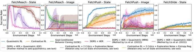
Figure 6: Online learning performance on GCRL benchmarks, including an alternative method to integrate quasimetrics in DDPG and a variant of Contrastive RL trained with two critics and exploration action noise on state-based settings. No method has access to ground truth reward function. QRL still consistently outperforms the baseline methods, learning both faster and better. FetchSlide with image observation is not shown because no method reaches a non-trivial success rate. See Section C.3 for details of the additional baselines.

Environment.    For FetchReach and FetchPush, we strictly follow Contrastive RL experimental setups (Eysenbach et al., 2022) to generate initial and goal states/images. The image observations are RGB with $64\times 64$ resolution. For FetchSlide, we adopt a similar strategy and generate goal states where object position dimensions are set to the target location and other dimensions are set to zeros. We are unable to get any method to reach a non-trivial success rate on FetchSlide with image observation despite tuning hyperparamteres and image rendering. We thus omit this setting in results.

Evaluation.    We evaluate each method for $50$ episodes every $2000$ environment steps (i.e., $40$ episodes). Following standard practice, we mark an episode as successful if the agent completes the task at any timestep within the time limit ($50$ steps). For clearer visualizations in Figures 5 and 6, the success rates curves are smoothed with a sliding window of length $5$ before gathering across $5$ seeds, similar to visualizations in (Liu et al., 2022). For comparing sample efficiencies between Contrastive RL and QRL, we look at the smoothed success rates from both methods, find the sample size where QRL first exceeds Contrastive RL’s final performance at $10^{6}$ samples, and compute the sample size ratio.

Processing Image Observations.    To process image inputs, all compared methods use the same backbone convolutional architecture from (Mnih et al., 2013) to encode the input image into a $1024$-dimensional flat vector. We adopt this approach from Contrastive RL (Eysenbach et al., 2022). For different modules in a method, each module uses an independent copy of this backbone (of same architecture but different set of parameters). For modules that takes in two observations (e.g., policy network in all methods and monolithic Q-functions in vanilla DDPG), the same backbone processes each input into a flat vector, and the concatenated $2048$-dimensional vector is fed into later parts of the module (which is usually an MLP). Other modules only take in a single observation and simply maps the processed $1024$-dimensional vector to the output in a fashion similar to the fully-connected head of convolutional nets (i.e., passing through an activation function and then an MLP). In architecture descriptions below, we omit this backbone part for simplicity, and use $x$ to denote the state dimension for state-based observations and backbone output dimension (i.e., $1024$) for image-based observations .

QRL (State-based Observations).    We use a $x$-512-512-128 network for $f$ and a (128+4)-512-512-128 residual network for $T$, where $4$ is the action dimension. For $d_{\theta}$, we use a 128-512-2048 projector followed by an IQE-maxmean head with $64$ components, each of size $32$. We use $x$-512-512-8 network for policy, where $x$ is the input size and $8$ parametrizes a tanh-transformed diagonal Normal distribution. $\mathcal{L}_{\mathsf{transition}}$ is optimized with a weight of $0.1$. Our learning rates are $0.01$ for $\lambda$, $1\times 10^{-4}$ for the model parameters, and $3\times 10^{-5}$ for the policy parameters. We use a batch size of $256$ in training. We prefill the replay buffer with $200$ episodes from a random actor, and then iteratively perform (1) generating $10$ rollouts and (2) optimizing QRL objective for $500$ gradients steps. We use $\mathcal{N}(0,0.3^{2})$-perturbed action noise in exploration. For the adaptive entropy regularizer (Haarnoja et al., 2018), we regularize policy to have target entropy $-\mathrm{dim}(\mathcal{A})$, where the entropy regularizer weight is initialized to be $1$ and optimized in log-space with a learning rate of $3\times 10^{-4}$. Since the environment has much shorter horizon (each episodes ends at $50$ timesteps), we instead use a different affine-transformed softplus for maximizing $d_{\theta}$, where $\phi(x)\triangleq-\mathrm{softplus}(15-x,\beta=0.1)$.

QRL (Image-based Observations).    All settings are the same as QRL for state-based observations except a few changes:

• We use the convolutional backbone followed by a $x$-512-128 network for encoder $f$.

• We optimize $\mathcal{L}_{\mathsf{transition}}$ with an increased weight of $10$ (since the dynamics aren’t fully deterministic).

• We update the models less frequently with $125$ gradient steps every $10$ rollouts. Contrastive RL uses the same reduced update frequency for image-based observations (Eysenbach et al., 2022), which we observe also has benefits for QRL.

Contrastive RL.    We strictly follow the original paper’s experiment settings (Eysenbach et al., 2022), which does not use two critics or action noise for exploration, and only uses entropy regularizer for image-based observations. For a comparison, we also run Contrastive RL with these techniques added on the state-based environments. As shown in Figure 6, while they do sometimes improve performance, they do not completely explain the gap between QRL and Contrastive RL. Hence, the improvement of QRL over Contrastive RL indeed (partly) comes from fundamental algorithmic differences. Since Contrastive RL estimates on-policy values, it could be more sensitive adding exploration noises, which degrades the dataset. QRL, however, is conceptually exempt from this issue, since it estimates optimal values.

Goal-Conditioned Behavior Cloning (GCBC).    We strictly follow the hyperparameter setups for the GCBC baseline in the Contrastive RL paper (Eysenbach et al., 2022).

DDPG + HER.    We mostly follow the experiment setup in the MRN paper (Liu et al., 2022). However, we do not give HER access to reward functions for fair comparison. Instead, HER relabels transition rewards based on whether the state equals the target goal state, which is exactly the same reward structure other method uses (QRL, Contrastive RL and GCBC).

DDPG + HER + Quasimetrics (Method by Liu et al. (2022)).    We strictly follow the MRN paper (Liu et al., 2022) to modify DDPG to include quasimetrics, which is slightly different from our modifications to Q-Learning on offline MountainCar, but was also shown to be empirically beneficial in online learning (Liu et al., 2022). We follow Liu et al. (2022) for MRN hyperparameters, and use the same IQE hyperparameters as QRL.

DDPG + HER + Quasimetrics (Another method to add quasimetrics).    We show additional results comparing QRL to a different approach to integrate quasimetrics into DDPG. This approach is different from the one by Liu et al. (2022) but similar to our modifications to Q-Learning on offline MountainCar that attain good performance in that task. We adapt the architecture choices by Liu et al. (2022) and QRL. Specifically, we use a $x$-512-512-128 network for encoder $f$ and (128+4)-512-512-128 residual network for $T$. For $d_{\theta}$, we use a 128-2048-2048-2048 projector followed by an IQE-maxmean head with $64$ components, each of size $32$. We adopt QRL’s transition loss with a weight of $5$. In other words, we replace the QRL’s value learning objective with the DDPG temporal-difference objective (and keep the transition loss). All other hyperparameters follow the same choices in method by Liu et al. (2022). This approach performs extremely poorly on this more challenging set of environments, suggesting that it is unable to scale to more complex continuous-control settings.

As shown in Figure 6, QRL greatly outperforms both approaches to integrate DDPG and quasimetrics, showing consistent advantage of the QRL objective over Q-Learning’s temporal-difference objective.

References

- Andrychowicz et al. (2017) Andrychowicz, M., Wolski, F., Ray, A., Schneider, J., Fong, R., Welinder, P., McGrew, B., Tobin, J., Pieter Abbeel, O., and Zaremba, W. Hindsight experience replay. Advances in neural information processing systems, 30, 2017.
- Bellemare et al. (2019) Bellemare, M., Dabney, W., Dadashi, R., Ali Taiga, A., Castro, P. S., Le Roux, N., Schuurmans, D., Lattimore, T., and Lyle, C. A geometric perspective on optimal representations for reinforcement learning. Advances in neural information processing systems, 32, 2019.
- Castro (2020) Castro, P. S. Scalable methods for computing state similarity in deterministic markov decision processes. In Proceedings of the AAAI Conference on Artificial Intelligence, volume 34, pp. 10069–10076, 2020.
- Chen et al. (2021) Chen, L., Lu, K., Rajeswaran, A., Lee, K., Grover, A., Laskin, M., Abbeel, P., Srinivas, A., and Mordatch, I. Decision transformer: Reinforcement learning via sequence modeling. Advances in neural information processing systems, 34:15084–15097, 2021.
- Denardo (1970) Denardo, E. V. On linear programming in a markov decision problem. Management Science, 16(5):281–288, 1970.
- D’Oro et al. (2023) D’Oro, P., Schwarzer, M., Nikishin, E., Bacon, P.-L., Bellemare, M. G., and Courville, A. Sample-efficient reinforcement learning by breaking the replay ratio barrier. In International Conference on Learning Representations, 2023.
- Durugkar et al. (2021) Durugkar, I., Tec, M., Niekum, S., and Stone, P. Adversarial intrinsic motivation for reinforcement learning. Advances in Neural Information Processing Systems, 34:8622–8636, 2021.
- Emmons et al. (2021) Emmons, S., Eysenbach, B., Kostrikov, I., and Levine, S. Rvs: What is essential for offline RL via supervised learning? arXiv preprint arXiv:2112.10751, 2021.
- Eysenbach et al. (2021) Eysenbach, B., Salakhutdinov, R., and Levine, S. Robust predictable control. arXiv preprint arXiv:2109.03214, 2021.
- Eysenbach et al. (2022) Eysenbach, B., Zhang, T., Salakhutdinov, R., and Levine, S. Contrastive learning as goal-conditioned reinforcement learning. arXiv preprint arXiv:2206.07568, 2022.
- Fan et al. (2022) Fan, L., Wang, G., Jiang, Y., Mandlekar, A., Yang, Y., Zhu, H., Tang, A., Huang, D.-A., Zhu, Y., and Anandkumar, A. Minedojo: Building open-ended embodied agents with internet-scale knowledge. In Thirty-sixth Conference on Neural Information Processing Systems Datasets and Benchmarks Track, 2022.
- Ferns & Precup (2014) Ferns, N. and Precup, D. Bisimulation metrics are optimal value functions. In UAI, pp. 210–219, 2014.
- Fu et al. (2020) Fu, J., Kumar, A., Nachum, O., Tucker, G., and Levine, S. D4rl: Datasets for deep data-driven reinforcement learning, 2020.
- Fu et al. (2021) Fu, X., Yang, G., Agrawal, P., and Jaakkola, T. Learning task informed abstractions. In International Conference on Machine Learning, pp. 3480–3491. PMLR, 2021.
- Fujimoto & Gu (2021) Fujimoto, S. and Gu, S. S. A minimalist approach to offline reinforcement learning. Advances in neural information processing systems, 34:20132–20145, 2021.
- Fujimoto et al. (2022) Fujimoto, S., Meger, D., Precup, D., Nachum, O., and Gu, S. S. Why should I trust you, Bellman? the Bellman error is a poor replacement for value error. arXiv preprint arXiv:2201.12417, 2022.
- Ghasemipour et al. (2022) Ghasemipour, S. K. S., Gu, S. S., and Nachum, O. Why so pessimistic? Estimating uncertainties for offline RL through ensembles, and why their independence matters. arXiv preprint arXiv:2205.13703, 2022.
- Ghosh et al. (2019) Ghosh, D., Gupta, A., Reddy, A., Fu, J., Devin, C., Eysenbach, B., and Levine, S. Learning to reach goals via iterated supervised learning. arXiv preprint arXiv:1912.06088, 2019.
- Haarnoja et al. (2018) Haarnoja, T., Zhou, A., Hartikainen, K., Tucker, G., Ha, S., Tan, J., Kumar, V., Zhu, H., Gupta, A., Abbeel, P., et al. Soft actor-critic algorithms and applications. arXiv preprint arXiv:1812.05905, 2018.
- Hafner et al. (2019) Hafner, D., Lillicrap, T., Ba, J., and Norouzi, M. Dream to control: Learning behaviors by latent imagination. arXiv preprint arXiv:1912.01603, 2019.
- Hart et al. (1968) Hart, P. E., Nilsson, N. J., and Raphael, B. A formal basis for the heuristic determination of minimum cost paths. IEEE transactions on Systems Science and Cybernetics, 4(2):100–107, 1968.
- Janner et al. (2021) Janner, M., Li, Q., and Levine, S. Offline reinforcement learning as one big sequence modeling problem. Advances in neural information processing systems, 34:1273–1286, 2021.
- Janner et al. (2022) Janner, M., Du, Y., Tenenbaum, J., and Levine, S. Planning with diffusion for flexible behavior synthesis. In International Conference on Machine Learning, 2022.
- Kingma & Ba (2014) Kingma, D. P. and Ba, J. Adam: A method for stochastic optimization. arXiv preprint arXiv:1412.6980, 2014.
- Kumar et al. (2019) Kumar, A., Peng, X. B., and Levine, S. Reward-conditioned policies. arXiv preprint arXiv:1912.13465, 2019.
- Kumar et al. (2020) Kumar, A., Zhou, A., Tucker, G., and Levine, S. Conservative Q-learning for offline reinforcement learning. Advances in Neural Information Processing Systems, 33:1179–1191, 2020.
- Lee et al. (2020) Lee, K.-H., Fischer, I., Liu, A., Guo, Y., Lee, H., Canny, J., and Guadarrama, S. Predictive information accelerates learning in rl. Advances in Neural Information Processing Systems, 33:11890–11901, 2020.
- Lillicrap et al. (2015) Lillicrap, T. P., Hunt, J. J., Pritzel, A., Heess, N., Erez, T., Tassa, Y., Silver, D., and Wierstra, D. Continuous control with deep reinforcement learning. arXiv preprint arXiv:1509.02971, 2015.
- Liu et al. (2022) Liu, B., Feng, Y., Liu, Q., and Stone, P. Metric residual networks for sample efficient goal-conditioned reinforcement learning. arXiv preprint arXiv:2208.08133, 2022.
- Lyle et al. (2022) Lyle, C., Rowland, M., Dabney, W., Kwiatkowska, M., and Gal, Y. Learning dynamics and generalization in reinforcement learning. arXiv preprint arXiv:2206.02126, 2022.
- Ma et al. (2022) Ma, Y. J., Sodhani, S., Jayaraman, D., Bastani, O., Kumar, V., and Zhang, A. VIP: Towards universal visual reward and representation via value-implicit pre-training. arXiv preprint arXiv:2210.00030, 2022.
- Mahadevan & Maggioni (2007) Mahadevan, S. and Maggioni, M. Proto-value functions: A Laplacian framework for learning representation and control in markov decision processes. Journal of Machine Learning Research, 8(10), 2007.
- Manne (1960) Manne, A. S. Linear programming and sequential decisions. Management Science, 6(3):259–267, 1960.
- Micheli et al. (2020) Micheli, V., Sinnathamby, K., and Fleuret, F. Multi-task reinforcement learning with a planning quasi-metric. arXiv preprint arXiv:2002.03240, 2020.
- Mnih et al. (2013) Mnih, V., Kavukcuoglu, K., Silver, D., Graves, A., Antonoglou, I., Wierstra, D., and Riedmiller, M. Playing Atari with deep reinforcement learning. arXiv preprint arXiv:1312.5602, 2013.
- Oord et al. (2018) Oord, A. v. d., Li, Y., and Vinyals, O. Representation learning with contrastive predictive coding. arXiv preprint arXiv:1807.03748, 2018.
- Paster et al. (2022) Paster, K., McIlraith, S., and Ba, J. You can’t count on luck: Why decision transformers fail in stochastic environments. arXiv preprint arXiv:2205.15967, 2022.
- Pearl (1984) Pearl, J. Heuristics: intelligent search strategies for computer problem solving. Addison-Wesley Longman Publishing Co., Inc., 1984.
- Pitis et al. (2020) Pitis, S., Chan, H., Jamali, K., and Ba, J. An inductive bias for distances: Neural nets that respect the triangle inequality. In Proceedings of the Eighth International Conference on Learning Representations, 2020.
- Plappert et al. (2018) Plappert, M., Andrychowicz, M., Ray, A., McGrew, B., Baker, B., Powell, G., Schneider, J., Tobin, J., Chociej, M., Welinder, P., et al. Multi-goal reinforcement learning: Challenging robotics environments and request for research. arXiv preprint arXiv:1802.09464, 2018.
- Roweis & Saul (2000) Roweis, S. T. and Saul, L. K. Nonlinear dimensionality reduction by locally linear embedding. science, 290(5500):2323–2326, 2000.
- Schaul et al. (2015) Schaul, T., Horgan, D., Gregor, K., and Silver, D. Universal value function approximators. In International conference on machine learning, pp. 1312–1320. PMLR, 2015.
- Sermanet et al. (2018) Sermanet, P., Lynch, C., Chebotar, Y., Hsu, J., Jang, E., Schaal, S., Levine, S., and Brain, G. Time-contrastive networks: Self-supervised learning from video. In 2018 IEEE international conference on robotics and automation (ICRA), pp. 1134–1141. IEEE, 2018.
- Sontag (1995) Sontag, E. An abstract approach to dissipation. In Proceedings of 1995 34th IEEE Conference on Decision and Control, volume 3, pp. 2702–2703. IEEE, 1995.
- Tenenbaum et al. (2000) Tenenbaum, J. B., De Silva, V., and Langford, J. C. A global geometric framework for nonlinear dimensionality reduction. science, 290(5500):2319–2323, 2000.
- Tian et al. (2020) Tian, S., Nair, S., Ebert, F., Dasari, S., Eysenbach, B., Finn, C., and Levine, S. Model-based visual planning with self-supervised functional distances. arXiv preprint arXiv:2012.15373, 2020.
- Wang et al. (2020) Wang, R., Foster, D. P., and Kakade, S. M. What are the statistical limits of offline RL with linear function approximation? arXiv preprint arXiv:2010.11895, 2020.
- Wang et al. (2021) Wang, R., Wu, Y., Salakhutdinov, R., and Kakade, S. Instabilities of offline rl with pre-trained neural representation. In International Conference on Machine Learning, pp. 10948–10960. PMLR, 2021.
- Wang & Isola (2020) Wang, T. and Isola, P. Understanding contrastive representation learning through alignment and uniformity on the hypersphere. In International Conference on Machine Learning, pp. 9929–9939. PMLR, 2020.
- Wang & Isola (2022a) Wang, T. and Isola, P. Improved representation of asymmetrical distances with interval quasimetric embeddings. In Workshop on Symmetry and Geometry in Neural Representations at Conference on Neural Information Processing Systems (NeurIPS 2022), 2022a.
- Wang & Isola (2022b) Wang, T. and Isola, P. On the learning and learnability of quasimetrics. In International Conference on Learning Representations, 2022b.
- Wang et al. (2022) Wang, T., Du, S. S., Torralba, A., Isola, P., Zhang, A., and Tian, Y. Denoised MDPs: Learning world models better than the world itself. In International Conference on Machine Learning. PMLR, 2022.
- Watkins (1989) Watkins, C. J. C. H. Learning from delayed rewards. 1989.
- Williams et al. (2015) Williams, G., Aldrich, A., and Theodorou, E. Model predictive path integral control using covariance variable importance sampling. arXiv preprint arXiv:1509.01149, 2015.
- Yang et al. (2020) Yang, G., Zhang, A., Morcos, A., Pineau, J., Abbeel, P., and Calandra, R. Plan2vec: Unsupervised representation learning by latent plans. In Learning for Dynamics and Control, pp. 935–946. PMLR, 2020.
- Yang et al. (2022) Yang, M., Schuurmans, D., Abbeel, P., and Nachum, O. Dichotomy of control: Separating what you can control from what you cannot. arXiv preprint arXiv:2210.13435, 2022.
- Zhang et al. (2020a) Zhang, A., McAllister, R., Calandra, R., Gal, Y., and Levine, S. Learning invariant representations for reinforcement learning without reconstruction. arXiv preprint arXiv:2006.10742, 2020a.
- Zhang et al. (2020b) Zhang, T., Guo, S., Tan, T., Hu, X., and Chen, F. Generating adjacency-constrained subgoals in hierarchical reinforcement learning. Advances in Neural Information Processing Systems, 33:21579–21590, 2020b.