Quantifying non-stabilizerness through entanglement spectrum flatness

Abstract

Non-stabilizerness - also colloquially referred to as magic - is the a resource for advantage in quantum computing and lies in the access to non-Clifford operations. Developing a comprehensive understanding of how non-stabilizerness can be quantified and how it relates other quantum resources is crucial for studying and characterizing the origin of quantum complexity. In this work, we establish a direct connection between non-stabilizerness and entanglement spectrum flatness for a pure quantum state. We show that this connection can be exploited to efficiently probe non-stabilizerness even in presence of noise. Our results reveal a direct connection between non-stabilizerness and entanglement response, and define a clear experimental protocol to probe non-stabilizerness in cold atom and solid-state platforms.

Introduction.— Simulating quantum states is in general very hard for classical computers. It is expected that the exact classical simulation of arbitrary quantum systems is inefficient, as the resource overhead exponentially grows with the size of the system [1]. For this reason, Feynman put forward the notion of a quantum computer [2], as only quantum devices would be able to simulate a generic quantum system efficiently, as later proven in [3].

Entanglement - one of the defining characteristics and essential resources for quantum processing and computing - has been thoroughly studied [4, 5, 6, 7, 8, 9, 10, 11]. However, probing entanglement in insufficient for quantum advantage, nor it is enough to characterize entanglement by a single number [12, 13, 14, 15, 16]. For instance, one can obtain highly entangled states by Clifford circuits [17] that can be efficiently simulated classically [18, 19, 20, 21]; moreover, entanglement complexity is revealed in the finer structure of the entanglement spectrum statistics[22, 23, 24]. Transitions between different classes of entanglement complexity are driven by non-Clifford resources [25, 26, 27, 28, 29, 30], which are indeed also the necessary resources to quantum advantage[31].

Any extension of Clifford circuits (that is, circuits only containing the Hadamard gate, the $\pi/2$-phase gate, and the controlled-Not gate) enables them to perform universal computation by allowing the input states to include the so-called magic states [32, 33, 34] that enable the distillation of a single-qubit unitary $T=\rm{diag}(1,e^{i\pi/4})$, which, added to the Clifford gates, makes a universal set of gates. Classical simulation of cirquits with $n$ qubits using a number $t$ of magic states scales as $\mbox{poly n}\exp{t}$ [20]: consequently, one can perform an efficient classical simulation for any circuit using only logarithmically many input magic-state qubits [35, 36, 37].

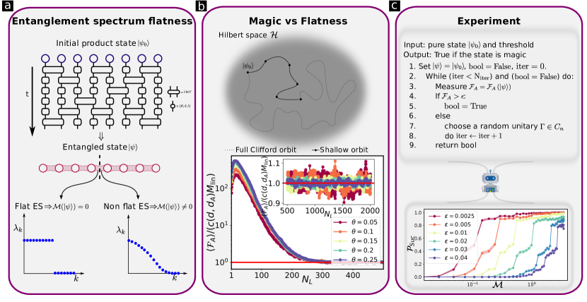
Figure 1: Summary of the results: (a) A schematic of the method to quantify the non-stabilizerness of a pure state. We start from a product state and then we apply random Clifford gates to obtain a volume-law entangled state. From the entanglement spectrum ES in any bipartition, we can distinguish whether the initial state possesses non-stabilizerness. (b) In the upper panel, a sketch of the Clifford orbit of a pure state is shown. In the lower panel, we show the ratio between flatness $\mathcal{F}_{A}$ and non-stabilizerness, quantified by $c(d,d_{A})M_{\rm{lin}}$. We initialize the system as a product state $|\psi(\theta)\rangle=\otimes^{n}_{i=1}|\psi(\theta)\rangle_{i}$ and $n=14$, for different values of $\theta$ and apply $N_{L}$ random Clifford layers. The ratio approaches $1$ in the limit of large $N_{L}$ as predicted by the theorem. (c) Algorithm to determine if a state is a stabilizer state or possesses some non-stabilizerness. We show the pseudocode in the upper part of the panel. In the lower part, we show the probability to catch a non-stabilizerness. We generate product states $|\psi(\theta)\rangle=\otimes^{n}_{i=1}|\psi(\theta)\rangle_{i}$ for $n=12$ qubits, and, we fix the number of Clifford layers $N_{L}=100$. After performing $N_{R}=1000$ realizations, we compute the probability of success $\mathcal{P}_{\rm{suc}}$ for different values of threshold, as a function of the initial value of non-stabilizerness in the initial state calculated using the second SRE.

As explained above, non-Clifford resources are necessary for any quantum advantage so they are a precious resource in quantum information processing, often dubbed non-stabilizerness, or, more colloquially, magic [34]. The resource theory for non-stabilizerness has been developed in the last few years. Most of the proposed measures are based on the discrete Wigner formalism [38, 39, 40, 41, 42, 43]. Prominent examples include the relative entropy of magic and the mana [21], the stabilizer rank [36, 35, 44], the robustness of magic [45, 46], the thauma [47], and the stabilizer extent [48]. Most of these quantifiers of non-stabilizerness are difficult to evaluate even numerically. One computable and practical measure of non-stabilizerness has been introduced recently: the Stabilizer Rényi Entropy (SRE) [49] can be computed efficiently for matrix product states [50, 51], is amenable to experimental measurement [52, 53] and has tight connections with quantum verification and benchmarking [54].

In this work, we establish a deep connection between the SRE and the flatness of the entanglement spectrum associated to a subsystem density operator. At the conceptual level, this connection shows clearly how this resource is associated with entanglement structure: non-stabilizerness is directly tied to entanglement response, a quantum analogue of ’heat capacity’ for thermodynamic systems. At the very same time, it opens the door for important practical applications. We present a simple practical protocol for experimentally probing this quantity efficiently inspecting density matrices of small bipartitions.

Our main findings are summarized in Fig. 1. In Fig. 1 (a), we show the set-up that we use utilize to make the connection between nonstabilizerness and entanglement response concrete: we prepare initial states as a product states and evolve them using random Clifford gates, followed by the measurement of the entanglement spectrum flatness. We find that a state possesses non-stabilizerness if and only if its entanglement spectrum is not flat. In the second panel (Fig. 1 (b)), we illustrate the Clifford orbit of a pure state: its non-stabilizerness is proportional to its average flatness over the orbit. Finally, in the third panel (Fig. 1 (c)), we present an algorithm for detecting non-stabilizerness and show the probability of success as a function of their degree of non-stabilizerness.

Stabilizer Rényi entropy and the flatness of entanglement spectrum.— In this section, we define the SRE and its connection with the flatness of the entanglement spectrum. In particular, we will show that we can quantify the non-stabilizerness of an arbitrary pure state by taking the average of the flatness along its Clifford orbit.

Consider the $d=2^{n}-$dimensional Hilbert space of $n$ qubits $\mathcal{H}\simeq\mathbb{C}^{\otimes 2n}$. A subset $\Lambda$ of the $n$ qubits with $|\Lambda|=n_{\Lambda}$ defines a subsystem with $d_{\Lambda}=2^{n_{\Lambda}}-$dimensional Hilbert space $\mathcal{H}_{\Lambda}\simeq\mathbb{C}^{\otimes 2n_{\Lambda}}$. Let $P_{i}\in\{I,X,Y,Z\}$ be the Pauli operators on the $i-$th single qubit space $\mathbb{C}^{2}$. Pauli operators on the full $\mathcal{H}$ have the form $P=\otimes_{i}^{n}P_{i}$ and local Pauli operators can be written also as $P_{X}=\otimes_{i\in\Lambda}P_{i}$. We call $\mathcal{P}_{n}$ be the group of all $n$-qubit Pauli operators with phases $\pm 1$ and $\pm i$, and define $\Xi(|\psi\rangle)=d^{-1}\langle\psi|P|\psi\rangle^{2}$ as the squared (normalized) expectation value of $P$ in the pure state $|\psi\rangle$ with $d=2^{n}$ the dimension of the Hilbert space of $n$ qubits. Moreover, $\Xi$ is the probability of finding $P$ in the representation of the state $|\psi\rangle$. Now we can define the SREs as:

$$M_{\alpha}\left(|\psi\rangle\right)=\frac{1}{1-\alpha}\log\left\{\sum_{P\in\mathcal{P}_{n}}\frac{\langle\psi|P|\psi\rangle^{2\alpha}}{d}\right\}\,.$$ (1)

The SRE is a good measure from the point of view of resource theory. Indeed, it has the following properties: (i) faithfulness $M_{\alpha}\left(|\psi\rangle\right)=0$ iff $|\psi\rangle\in\rm{STAB}$, otherwise $M_{\alpha}(|\psi\rangle)>0$, (ii) stability under Clifford operations: $\forall\Gamma\in C_{n}$ we have that $M_{\alpha}\left(\Gamma|\psi\rangle\right)=M_{\alpha}\left(|\psi\rangle\right)$ and (iii) additivity $M_{\alpha}\left(|\psi\rangle\otimes|\phi\rangle\right)=M_{\alpha}\left(|\psi\rangle\right)+M_{\alpha}\left(|\phi\rangle\right)$ (the proof can be found in [49], see also [55]). Another useful measure of non-stabilizerness is given by the stabilizer linear entropy, defined as

$$M_{\rm{lin}}(|\psi\rangle):=1-d||\Xi(|\psi\rangle)||^{2}_{2},$$ (2)

which obeys the following properties: (i) faithfulness $M_{\rm{lin}}\left(|\psi\rangle\right)=0$ iff $|\psi\rangle\in\rm{STAB}$, otherwise $M_{\rm{lin}}(|\psi\rangle)>0$, (ii) stability under Clifford operations: $\forall\Gamma\in C_{n}$ we have that $M_{\rm{lin}}\left(\Gamma|\psi\rangle\right)=M_{\rm{lin}}\left(|\psi\rangle\right)$ and (iii) upper bound $M_{\rm{lin}}<1-2\left(d+1\right)^{-1}$. The relationship between the second SRE $M_{2}$ and the linear non-stabilizing entropy follows easily from $M_{2}=\log\left(1-M_{\rm{lin}}\right)$.

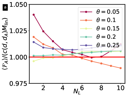
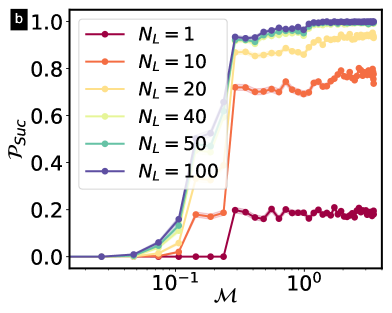
Figure 2: (a) Numerical simulations of shallow circuits: Plot the ratio $\mathcal{F}_{A}/c(d,d_{A})M_{\rm{lin}}$ vs $N_{L}$ for a shallow circuit starting from a state in the volume phase. (b) Probability of success $\mathcal{P}_{\rm{Suc}}$ vs the initial value of non-stabilizerness $M_{(2)}\left(|\psi_{0}\rangle\right)$ for a fixed threshold $\epsilon=0.005$ and for different $N_{L}$. $\mathcal{P}_{\rm{Suc}}$ computed over $N_{\text{R}}=1000$ realizations.

Let us now discuss the relationship between the SRE and the flatness of the entanglement spectrum. Consider a pure state $\psi$ in a bipartite system $\mathcal{H}=\mathcal{H}_{A}\otimes\mathcal{H}_{B}$ and its reduced density operator $\psi_{A}=\text{Tr}_{B}\psi$. The flatness of its entanglement spectrum is defined as

$$\mathcal{F}_{A}(\psi):=\text{Tr}\left(\psi^{3}_{A}\right)-\text{Tr}^{2}\left(\psi^{2}_{A}\right)$$ (3)

One can easily check that $\mathcal{F}_{A}(\psi)=0$ iff the entanglement spectrum is flat, i.e. if the spectrum $\lambda_{\alpha}=1/\chi$ for some integer $1\leq\chi\leq\rm{min}\left(d_{A},d_{B}\right)$, whereas $\mathcal{F}_{A}\left(|\psi\rangle\right)>0$ in other cases. In this context, we use the flatness of entanglement spectrum to quantify non-stabilizerness of a pure state.

Theorem: The Stabilizer Linear Entropy $M_{\rm{lin}}$ of a pure state $|\psi\rangle)$ is proportional to the flatness of the entanglement spectrum averaged over the Clifford orbit:

$$\langle\mathcal{F}_{A}(\Gamma\ket{\psi})\rangle_{C_{n}}=c(d,d_{A})M_{\rm{lin}}(|\psi\rangle)\,,$$ (4)

where $\langle\cdot\rangle_{C_{n}}$ denotes the average over the Clifford orbit $\Gamma\ket{\psi}$ and the proportionality constant $c(d,d_{A})\sim(d^{2}-d^{2}_{A})d^{-3}$ for large $d$, see [56] for the proof.

Notice that the above result holds true for any bipartition of the system, which is reflected in the constant $c(d,d_{A})$. We see that a pure stabilizer state possesses flat entanglement spectrum over all its Clifford orbit and flatness is stable under Clifford operations. Moreover, one can utilize a measurement of flatness to measure $M_{\rm{lin}}$.

Numerical experiments.—

As it was shown in [53], SRE can be experimentally measured via randomized unitaries [57], providing an important handle on the quality of a quantum circuit. However, SRE is a very expensive quantity to measure, requiring in general exponential resources (though better than state tomography). The result of the opens the way to a very efficient way to measure SRE. However, things are not so simple. In the best case scenario, $c(d,d_{A})=O(d^{-1})$, which means that one needs to resolve an exponentially small quantity, thereby requiring again exponential resources - even if with the considerable advantage that operations on a small subset are needed, thus relaxing one of the most challenging requirements of previous methods. This is because $\psi_{A}$ is typically very entangled over $C_{n}$ and therefore $\mathcal{F}_{A}$ is very close to be flat. A very long circuit (inevitably, very sensitive to noise) will thus be required in those cases. Another issue is that, for weakly entangled states, a direct exploitation of the theorem is extremely challenging in practise, as we shall demonstrate numerically in the following. One can intuitively understand that as for very weakly entangled states there are very few eigenvalues at all in the entanglement spectrum, think of the spectrum of a product state.

The key insight is that we can get around the requirement of a full Clifford orbit by (numerically) analyzing the intermediate regime approaching volume law one might be able to see a deviation from flat spectrum without having to resolve an exponentially small quantity. If this is true, one would have found a witness for non-stabilizerness that is efficiently computable and measurable. Moreover, as one gets in the volume law for entanglement phase, one should be able to evaluate accurately the actual value of $M_{lin}$, even without averaging over all the Clifford orbit. Of course, in this case one still needs to resolve a very small quantity.

We consider an initial state that is a product state of $n$ qubits with linear topology $|\psi(\theta)\rangle=\otimes^{n}_{i=1}|\psi_{i}(\theta)\rangle\equiv 2^{-n/2}\left(|0\rangle+e^{i\theta}|1\rangle\right)_{i}$ with $M_{2}(\theta)=n[1-\log(1+\sin^{4}\theta+\cos^{4}\theta)]$. The state $|\psi(\theta)\rangle$ is then evolved under a random Clifford circuit of depth $N_{L}$ denoted by $U_{\rm{Cl}}=\prod_{k}^{N_{L}}U_{k}$, where $U_{k}$ contains $n-1$ Clifford gates (Hadamard, phase $e^{i\pi/2}$ gate and CNOT)[17] between nearest neighbors.

We study the flatness $\langle\mathcal{F}_{A}\rangle$ of the reduced density matrix $\rho_{A}=\text{Tr}_{B}|\psi(t)\rangle\langle\psi(t)|$ (for $d_{A}=d_{B}=2^{n/2}$ and $n=14$ qubits) under random Clifford circuit evolution. In Fig. 1 (b), we present the average flatness $\langle\mathcal{F}_{A}\rangle$ as a function of the circuit depth $N_{L}$. The average is obtained from $N_{R}=1000$ different realizations and it is calculated for various values of $\theta$. For a small number of Clifford layers, the flatness increases and exhibits a sharp dependence on $\theta$. When the circuit is very deep, the system explores a very large portion of its Clifford orbit, and the ratio between average flatness $\langle\mathcal{F}_{A}\rangle$ and $c(2^{n},2^{n/2})M_{\rm{lin}}$ approaches 1 (the solid red line in the inset of Figure 1), as predicted by the Theorem.

In Fig. 2(a), we show that one can accurately estimate $M_{lin}$ even by shallow Clifford circuits provided one starts with volume law entanglement. We again consider a $n=14$ qubit system in a volume law phase by subjecting the initial state $|\psi(0)\rangle$ to $N_{L}=1500$ Clifford layers, for various values of $\theta$. We then plot the ratio $\langle\mathcal{F}_{A}\rangle/c(2^{n},2^{n/2})M_{\rm{lin}}$ as a function of the number of Clifford $N_{L}$. The theoretical line predicted by the theorem is shown as a solid red line. Notably, we observe that even for circuits as short as $N_{L}=7$ Clifford layers, the average flatness reaches the value predicted by the theorem [58].

Probing non-stabilizerness through flatness. —

As we discussed above, one could probe non-stabilizerness by probing flatness, which is is amenable to be measured in experiments [59, 60, 61]. However, a naïve application of the theorem would result in a very costly procedure. We present an algorithm that can efficiently probe magic by exploring the Clifford orbit in the intermediate region between weak and volume-law entanglement [58].

The procedure works as follows: (1) Start with $|\psi_{0}\rangle$, a pure state. (2) Draw a random Clifford gate $\Gamma$ and apply it to the initial state: $|\psi_{\Gamma}\rangle\equiv\Gamma|\psi_{0}\rangle$. (3) Measure the entanglement spectrum flatness $\mathcal{F}_{A}(\psi_{\Gamma})$. For small partitions, this can be done either via state tomography, or utilizing the random unitary toolbox [57]. If the original state $|\psi_{0}\rangle$ is a stabilizer state, the output of the circuit is still a stabilizer state with zero flatness. On the contrary, if $|\psi_{0}\rangle$ has a non-vanishing amount of non-stabilizerness, we expect that even a modest exploration of the Clifford orbit will result into a non flat entanglement spectrum. Therefore, if after a number of Clifford unitaries we measure $\mathcal{F}_{A}>0$ we can establish that the initial state possesses non-stabilizerness. The resulting algorithm is summarized in Fig. 1 (c). In this algorithm, we set both the number of iterations (which determines the number of Clifford layers) and the threshold for measuring flatness.

Notably, our proposed protocol does not demand an exhaustive exploration of the Clifford group, which is exponentially large. Instead, our findings in the previous section demonstrate that a shallow quantum circuit generated by fixing the number of Clifford layers to a reasonably small value is sufficient for detecting non-stabilizerness with a high probability. This is illustreated in Fig. 1 (c): we show the probability of success $\mathcal{P}_{\rm{Suc}}$ (for $n=12$ qubits) as a function of the initial value of non-stabilizerness calculated using the second SRE defined in Eq.(1). In order to address the role of errors in the measurement of $\mathcal{F}_{A}$, we introduce a thresholdvalue $\epsilon$ for our test. The success probability is defined as the number of times in which the algorithm gives True as output, thus detecting the non-stabilizerness of the initial state normalized to the total number of iterations. In Fig. 2 (b), we present the probability of success $\mathcal{P}_{\rm{Suc}}$ (for $n=12$ qubits) for a different maximum number of Clifford layers $N_{L}$. We fix the threshold $\epsilon=0.005$ and we compute the probability as a function of non-stabilizerness calculated by $M_{(\alpha)}\left(|\psi_{0}\rangle\right)$ of the initial state. The plot shows that increasing the number of algorithmic iterations $N_{L}$ pushes the probability of success to $1$ for any fixed values of non-stabilizerness.

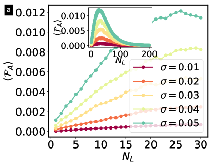
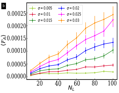
Figure 3: Flatness in noisy circuit: (a) We show the average of the flatness, over $N_{\rm{R}}=1000$ realizations, as a function of $N_{L}$. Starting from STAB state $|+\rangle^{\otimes n}$ magic is injected by a perturbed CNOT gate resulting in increasng flatness $\mathcal{F}_{A}$. (b) Average flatness over $N_{\rm{R}}=1000$ realizations as a function $N_{L}$. The system is initialized in the ground state of Toric code, on a $4\times 2$ unit cell (16 spins). The flatness increases almost linearly with the number of Clifford layers $N_{L}$. Error bars correspond to a $95\%$ confidence interval.

Noisy Clifford circuit.—

So far we assumed that Clifford unitaries are ideal. In reality, they have a residual noise. In this situation, it is more natural to perform error mitigation at the level of channels rather than states. Consider a simple error model where each two-qubit Clifford $V$ is independently affected by a unitary noise $\tilde{V}=e^{-i\sum_{\alpha}\epsilon_{\alpha}\sigma^{\alpha}}Ve^{i\sum_{\alpha}\epsilon_{\alpha}\sigma^{\alpha}}$, where $\epsilon_{\alpha}$ is a random number chosen from a Gaussian distribution with average zero and standard deviation $\sigma$ that represents here the strength of the noise.

Introducing noise to Clifford gates represents a magic-state injection that can be accurately captured by computing the flatness $\mathcal{F}_{A}$. In Fig. 3 (a) we present the evolution of the flatness $\mathcal{F}_{A}$ for a noisy Clifford circuit with $n=14$ qubits. We initialize the system in the global stabilizer state $|+\rangle$ and compute the flatness after every Clifford layer. Moreover, we also investigate the effect of noise starting from the ground state of the toric code - a stabilizer code formulated on a square lattice [62, 63, 64, 65]. The basic construction of the toric code is a square lattice with a spin-$1/2$ degree of freedom on every bond, the physical qubits. The model is given in terms of a Hamiltonian $\hat{H}=-\sum_{\nu}A_{\nu}-\sum_{p}B_{p}$, where $\alpha$ runs over all plaquettes and $\nu$ over all vertices (sites). The ground state of the toric code is a stabilizer state of the sets $\left\{A_{\nu}\right\}$ and $\left\{B_{p}\right\}$. After applying a Clifford circuit with a transformed CNOT gate, we compute $\mathcal{F}_{A}$ after every layer. In Fig. 3 (b) we show the evolution of $\mathcal{F}_{A}$ for different strengths of noisy $\sigma$. It increases almost linearly with the number of Clifford layers. These results quantify how, upon close inspection of the microscopic imperfections, it is possible to define an error threshold that is able to discriminate between magic injected by errors along the Clifford orbit, and intrinsic magic of the original state.

Conclusions.—

We have demonstrated how non-stabilizerness of quantum states, while completely unrelated to entanglement per se, is deeply and exactly related to entanglement response, via the entanglement spectrum flatness of arbitrary partitions. Leveraging on this connection, we have formulated a simple protocol to efficiently witness and quantify non-stabilizerness in quantum systems, that is applicable to both atom and solid state settings where local operations and probing is available. The protocol is particularly efficient for states with volume law entanglement, and can cope with the unavoidable presence with noise, as we demonstrate utilizing both random states and toric code dynamics. Our results paves the way for witnessing nonstabilizerness in large scale experiments - a pivotal step to demonstrate computational advantage -, and motivates further study of non-stabilizerness in quantum many-body systems, in particular, in connection to critical behavior, where entanglement response is expected to be particularly relevant.

I Supplemental Material

I.1 Proof of Theorem 1

Let us recall the measure of entanglement spectrum flatness for a pure state $\ket{\psi}$ in the bipartition $A\cup B$ defined in the main text

$$\mathcal{F}_{A}(\ket{\psi})=\operatorname{Tr}(\rho_{A}^{3})-\operatorname{Tr}^{2}(\rho_{A}^{2})$$ (5)

where $\rho_{A}=\operatorname{Tr}_{B}\ket{\psi}\!\!\bra{\psi}$. In this section, we compute the average over the Clifford orbit $\Gamma\ket{\psi}$ where $\Gamma\in C_{n}$, i.e. $\braket{\mathcal{F}_{A}(\Gamma\ket{\psi})}_{C_{n}}$. Note that we can write

$$\braket{\mathcal{F}_{A}(\Gamma\ket{\psi})}_{C_{n}}=\braket{\operatorname{Tr}(\rho_{\Gamma,A}^{3})}_{C_{n}}-\braket{\operatorname{Tr}^{2}(\rho_{\Gamma,A}^{2})}_{C_{n}}$$ (6)

where $\rho_{\Gamma,A}=\operatorname{Tr}_{B}(\Gamma\ket{\psi}\!\!\bra{\psi}\Gamma^{{\dagger}})$. We can now use the swap trick, i.e. $\operatorname{Tr}(O^{3})=\operatorname{Tr}(T_{(123)}O^{\otimes 3})$ and $\operatorname{Tr}^{2}(O^{2})=\operatorname{Tr}(T_{(12)(34)}O^{\otimes 4})$ to linearize the above averages over multiple copies of $\ket{\psi}$

$$\braket{\mathcal{F}_{A}(\Gamma\ket{\psi})}_{C_{n}} = \operatorname{Tr}(T_{(123)}^{A}\braket{(\Gamma\ket{\psi}\!\!\bra{\psi}\Gamma^{{\dagger}})^{\otimes 3}}_{C_{n}})$$

$$- \operatorname{Tr}(T_{(12)(34)}^{A}\braket{(\Gamma\ket{\psi}\!\!\bra{\psi}\Gamma^{{\dagger}})^{\otimes 4}}_{C_{n}})$$

where $T_{(123)}^{A}$ and $T_{(12)(34)}^{A}$ are permutations acting non-identically on the subsystem $A$ only. For the first average in the r.h.s. of Eq. (I.1), we use the fact that the Clifford group is a $3$-design [66, 67] and thus

$$\braket{(\Gamma\ket{\psi}\!\!\bra{\psi}\Gamma^{{\dagger}})^{\otimes 3}}_{C_{n}}=\frac{\Pi^{(3)}_{sym}}{d(d+1)(d+2)}$$ (8)

where $\Pi^{(3)}_{sym}=\sum_{\pi_{3}\in S_{3}}T_{\pi_{3}}$ is the symmetric projector, $S_{3}$ is the symmetric group acting on $3$ copies of the Hilbert space of $n$ qubits and $T_{\pi_{3}}$ are unitary representations of permutations $\pi_{3}\in S_{3}$. For the second average of the r.h.s. of Eq. (I.1), we use the technical results presented in [26, 27] that shows

$$\braket{(\Gamma\ket{\psi}\!\!\bra{\psi}\Gamma^{{\dagger}})^{\otimes 4}}_{C_{n}} = \alpha Q\Pi_{sym}^{(4)}+\beta\Pi_{sym}^{(4)}$$ (9)

where $Q=d^{-2}\sum_{P\in\mathcal{P}_{n}}P^{\otimes 4}$ and $\Pi^{(4)}_{sym}$ is the symmetric projector on $S_{4}$, defined in the same fashion of $\Pi_{sym}^{(3)}$. Then we defined

$$\alpha := \frac{|\!|\Xi(\ket{\psi})|\!|_{2}^{2}}{(d+1)(d+2)/6}-\beta$$

$$\beta := \frac{1-|\!|\Xi(\ket{\psi})|\!|_{2}^{2}}{(d^{2}-1)(d+2)(d+4)/24}$$ (10)

After a straightforward algebra, recalling that $M_{lin}(\ket{\psi})=1-d|\!|\Xi(\ket{\psi})|\!|_{2}^{2}$, one finds:

$$\langle\mathcal{F}_{A}(\operatorname{Tr}_{A}(C\ket{\psi}\bra{\psi}C^{{\dagger}}))\rangle_{C} = \frac{(d^{2}-d_{A}^{2})(d_{A}^{2}-1)}{(d^{2}-1)(d+2)d_{A}^{2}}M_{lin}(\ket{\psi})$$ (11)

$$\equiv c(d,d_{A})M_{lin}(\ket{\psi})$$

which concludes the proof.∎