Holographic MIMO Communications exploiting the Orbital Angular Momentum

Abstract

This study delves into the potential of harnessing the orbital angular momentum (OAM) property of electromagnetic waves in near-field and line-of-sight scenarios by utilizing large intelligent surfaces, in the context of holographic multiple-input multiple-output (MIMO) communications. The paper starts by characterizing OAM-based communications and investigating the connection between OAM-carrying waves and optimum communication modes recently analyzed for communicating with smart surfaces. Subsequently, it proposes implementable strategies for generating and detecting OAM-based communication signals using intelligent surfaces and optimization methods that leverage focusing techniques. Then, the performance of these strategies is quantitatively evaluated through simulations. The numerical results show that OAM waves while constituting a viable and more practical alternative to optimum communication modes are sub-optimal in terms of achievable capacity.

I Introduction

The ceaseless quest for high-speed, reliable, and ubiquitous wireless services is leading today’s radio networks to their utmost. Fifth-generation (5G) wireless networks, exploiting the most advanced radio technologies, e.g., multiple-input multiple-output (MIMO) communications, have already been deployed in many countries and are establishing themselves as essential techniques to manage the ever-increasing number of devices’ connections. However, it is foreseen that sixth-generation (6G) wireless networks will push these requirements to the ultimate limit, introducing even more stringent requisites regarding user throughput, latency, scalability, and reliability, paving the way for massively novel applications and use cases. In this framework, the exploitation of higher operating frequencies, where a more considerable amount of spectral resources is available, in conjunction with the usage of large antenna arrays and antennas densification, has been envisaged as a potential, beneficial approach to tackle the challenging prerequisites that have been outlined. Nevertheless, the adoption of millimeter wave (mmWave) communications and terahertz technologies entails larger path loss, increased susceptibility to atmospheric turbulence, and in some cases, failure of traditional electromagnetic (EM) propagation models based on the far-field assumption. Indeed, when the antenna size becomes large or the frequency increases, the interaction between the transmitting and receiving antennas can occur in the radiating near-field region [2, 3]. Here the plane wave approximation of the wavefront becomes inapplicable, and the actual spherical-shaped wavefronts must be considered instead. This operating regime has been addressed as particularly favorable since it commences new and unexplored opportunities for future wireless systems, whose primary goal is to approach greater link-level spectrum efficiencies and unprecedented performance. From all the considerations above, the concept of holographic communications emerged [4, 5, 6], which can be referred to as the capability to utterly manipulate the EM field that is generated or received by antennas to exploit the entirety of the available channel’s degrees of freedom (DoF) and hence increase the communication capacity of the wireless link, even in line-of-sight (LOS) channel conditions. Specifically, previous work targeted the exploitation of large intelligent surface (LIS) antennas as transmitting and receiving devices in the near field, thus presenting a more comprehensive description of the communication problem in terms of communication modes, i.e., parallel channels that can be obtained between a couple of antennas at EM level [7, 8]. For instance, in [8], the optimal basis functions determining the optimum communications modes and their number, i.e., the available DoF, that can be established between two LISs have been obtained from solving an eigenfunction problem [7].

On another side, in the last decade, several works investigated the possibility of exploiting the orbital angular momentum (OAM) property of the EM waves to theoretically unfold further orthogonal radio channels. Initially, this was thought of as a new dimension to improve the DoF in wireless communications that is entirely independent of concepts like time, space, frequency, and polarization. Consequently, many relevant applications exploiting OAM have been envisaged in the latest years, and an extensive number of possible technologies and deployments have been proposed. For instance, a novel type of space-division multiplexing technique based on modes’ orthogonality has been theorized, namely OAM mode division multiplexing (OAM-MD) [9]. In addition, the possibility of managing the increasing users’ density through an OAM-based multiple access scheme (OAM-MDMA) was proposed as well [10]. Several other use cases have been investigated [11, 12, 13, 14, 15, 16] and, intuitively, many open issues and problems are still to be addressed since systems performance has been shown [17] to be strongly affected by the kind of antenna that is used, the overall systems architecture, the operating frequency, and many other elements. In spite of the initial enthusiasm in OAM, various investigations highlighted that substantial advantages with regard to more traditional techniques, such as MIMO communications, cannot be obtained by exploiting the OAM property of the radio waves [18, 19, 20, 21, 22].

OAM, whose employment was first studied in the optic domain [23, 24] and then also proposed for radio communications [25, 26], is frequently characterized by the use of specific beams, such as that corresponding to Laguerre-Gaussian (LG) modes [27, 23]. However, these modes are often considered without accounting for the specific transmitting and receiving devices, i.e., without considering particular antenna structures. In fact, a plethora of radio OAM generation methods have been identified [17], e.g., spiral phase plate (SPP) antennas, uniform circular arrays, and metasurfaces, and each of them was identified as optimal for a specific operating frequency. Indeed, it was shown that spiral reflectors and UCAs work best at radio-frequency (RF) and are more suitable for long-range transmissions, while SPPs and metasurfaces are better for the mmWaves band [17]. Nevertheless, the relationship among these LG modes and the concept of optimum communication modes discussed in [7, 8] is often unclear, as well as the gap between the DoF that can be obtained with OAM and those corresponding to the optimum strategy.

Numerous studies to date on OAM-based wireless systems contemplate the usage of UCAs as transmission and reception devices [28, 29, 30, 31]. However, these systems suffer from severe limitations in terms of hardware flexibility and phase quantization errors. In this regard, recent research [32, 33, 34, 35, 36] has demonstrated, both theoretically and experimentally, the feasibility and benefits of exploiting OAM in wireless systems by utilizing metasurfaces, especially in the terahertz band [37, 38, 39, 40, 41] where most of the propagation occurs in the near-field region of the transmitter. To the best of the authors’ knowledge, no analytical studies have addressed the use of OAM, or more in general, arbitrary EM phase and amplitude profiles, independently of the particular hardware implementation or antenna technology, as we instead perform by adopting homogenized, spatially continuous surfaces such as LISs.

In this work, motivated by the recent advancements concerning the communication between LISs, we revise the exploitation of OAM-based techniques as orthogonal communication channels. The proposed approach allows the investigation of the OAM capabilities in terms of capacity achievements and effectiveness, especially in relation to optimal strategies for defining the communication modes between a couple of antennas. The main contributions of the paper can be summarized as follows:

• Review of the concept of OAM communication in the framework of holographic MIMO and in relationship with communication modes;

• Characterization of the gap between OAM-based strategies and optimum communication modes for different configurations in terms of DoF;

• Proposal of the exploitation of beam focusing for reducing the typical divergence effects of OAM beams within the near-field (Fresnel) region, showing the related benefits and drawbacks;

• Proposal and analysis of different detection strategies for the implementation of OAM-based receivers;

• Discussion of the main advantages and disadvantages concerning the exploitation of OAM in the holographic MIMO scheme.

The remainder of the paper is organized as follows: Section II revises the concept of communication between LISs and introduces the notion of communication modes, thus discussing the adoption of optimal transmitting and receiving basis function sets. Section III describes the characteristics of OAM propagation. Then, the relationship between OAM and optimum communication modes is illustrated, and the characteristics of OAM modes are discussed. In Section IV the overall OAM-based communication scheme is presented, and beam focusing within the near-field is introduced as a way to improve the system performance. Then, in Section. V practical detection strategies are presented, while Section VI illustrates some numerical results to characterize the gap between OAM communications and optimum strategies. Finally, a discussion concerning the main strengths and weaknesses of using OAM-based radio communications, together with an implementation complexity analysis, is provided, and Section VII concludes the paper.

II Communications with LISs

LISs can be denoted as active, re-configurable planar antennas whose sizes are much larger than the operating wavelength, that can control the amplitude and phase profiles of the EM waves with high flexibility and resolution. Notably, metamaterials have been proposed [42, 43, 44] as a viable technology to create those kinds of antennas, thus enabling the design of predefined EM waves’ features in terms of shape, polarization, and steering. From an analytical viewpoint, LISs can be abstractly modeled as continuous surfaces composed of an infinite number of sub-wavelength antenna elements, regardless of their specific hardware implementation. Research in [8] has investigated the fundamental limitations of communication using LISs, showing that by carefully designing the amplitude and phase profiles of the transmitting and receiving LISs, multiple communication modes, known as channel’s DoF, can be achieved in LOS near-field conditions. Particularly, these communication modes can be seen as a collection of parallel, orthogonal channels at EM level, which allows for the capability to spatially multiplex signals within the wireless system. In the following subsection, the formal definition of communication modes is briefly revised. The reader can refer to [7, 8] for a complete treatment.

II-A Communication Modes

Abstracting in the first instance from the specific shape or antennas’ configuration, let us generally consider a transmitting and a receiving LIS of area $S_{\text{T}}$ and $S_{\text{R}}$. We indicate with $\textbf{s}\in S_{\text{T}}$ and $\textbf{r}\in S_{\text{R}}$ the vectors pointing from the origin of the contemplated reference system towards a point on the transmitting and the receiving LIS, respectively. A monochromatic source at frequency $f_{0}$, i.e., $\phi(\textbf{s})$, is used at the transmitting LIS. This source generates a wave function $\psi(\textbf{r})$ at the receiving antenna, which is a solution of the inhomogeneous Helmholtz equation

$$\nabla^{2}\psi(\mathbf{r})+\kappa^{2}\psi(\mathbf{r})=-\phi(\mathbf{s})\,.$$ (1)

A solution of (1) in free-space propagation condition is provided as

$$\psi(\textbf{r})=\int_{S_{\text{T}}}G(\textbf{r},\textbf{s})\phi(\textbf{s})\,\text{d}\textbf{s}$$ (2)

where the scalar Green function $G(\mathbf{r}_{1},\mathbf{r}_{2})$ between the points represented by the vectors $\mathbf{r}_{1}$ and $\mathbf{r}_{2}$ is given by

$$G\left(\mathbf{r}_{1},\mathbf{r}_{2}\right)=\frac{\exp\left(-\jmath\kappa\left|\left|\mathbf{r}_{1}-\mathbf{r}_{2}\right|\right|\right)}{4\pi\left|\left|\mathbf{r}_{1}-\mathbf{r}_{2}\right|\right|}$$ (3)

where $\kappa=2\pi/\lambda$ is the free-space wavenumber and $\lambda=c/f_{0}$ indicates the wavelength, with $c$ being the light speed. It is important to note that in (3), the reactive field components that typically vanish for link distances greater than a few wavelengths are neglected, as the system is supposed to operate in the radiating near-field region.

In the following, we will treat the EM field as a complex-valued scalar quantity (e.g., by considering a single polarization), despite being a vectorial complex quantity. This simplification does not affect the generality or validity of the results, which can be extended to the vectorial case. Formally, communication modes can be described by the mean of specific orthonormal basis expansions of the transmitting function $\phi(\textbf{s})$ and receiving function $\psi(\textbf{r})$, respectively denoted by ${\phi_{n}(\textbf{s})}$ and ${\psi_{n}(\textbf{r})}$, where $n=1,2,...,\infty$. If the basis sets are devised such that exists a bijective relationship among the $n$-th transmitting basis function $\phi_{n}(\textbf{s})$ and the $n$-th receiving one $\psi_{n}(\textbf{r})$, the existence of multiple communication modes is ensured. In this case, each transmitting function $\phi_{n}(\textbf{s})$ induces an effect $\xi_{n}\psi_{n}(\textbf{r})$ on the receiving antenna, with $\xi_{n}$ identifying the largest feasible coupling coefficient. Precisely, large $\xi_{n}$ coefficients indicate well-coupled modes, i.e., pair of functions ($\phi_{n}(\textbf{s})$, $\psi_{n}(\textbf{r})$), between transmitting and receiving LISs corresponding to practicable, parallel communication channels; small $\xi_{n}$ instead, denotes the prevalence of the wave’s dispersion away from the receiver. In addition, the linear combinations of $\phi_{n}(\mathbf{s})$ and $\psi_{n}(\mathbf{r})$ functions are proportional to the current spatial distribution impressed on the transmitting LIS, and to the resulting electric field at the receiving LIS side, respectively, thus the latter is referred as $n$-th electric field component in the following.

In principle, infinite basis sets are realizable, but to achieve the highest number of communication modes with the largest coupling, the following coupled eigenfunction problem needs to be solved, thus leading to the optimal basis functions [7, 8]

$$\xi_{n}^{2}\,\phi_{n}(\textbf{s})=\int_{S_{\text{T}}}K_{\text{T}}(\textbf{s},\textbf{s}^{\prime})\,\phi_{n}(\textbf{s}^{\prime})\,\text{d}\textbf{s}^{\prime}$$ (4)

$$\xi_{n}^{2}\,\psi_{n}(\textbf{r})=\int_{S_{\text{R}}}K_{\text{R}}(\textbf{r},\textbf{r}^{\prime})\,\psi_{n}(\textbf{r}^{\prime})\,\text{d}\textbf{r}^{\prime}$$ (5)

where the kernels $K_{\text{T}}(\textbf{s},\textbf{s}^{\prime})$ and $K_{\text{R}}(\textbf{r},\textbf{r}^{\prime})$ are given by

$$K_{\text{T}}(\textbf{s},\textbf{s}^{\prime})=\int_{S_{\text{R}}}G^{*}(\textbf{r},\textbf{s})G(\textbf{r},\textbf{s}^{\prime})\,\text{d}\textbf{r}$$ (6)

$$K_{\text{R}}(\textbf{r},\textbf{r}^{\prime})=\int_{S_{\text{T}}}G(\textbf{r},\textbf{s})G^{*}(\textbf{r}^{\prime},\textbf{s})\,\text{d}\textbf{s}\;.$$ (7)

Determining these solutions can be very challenging and may require a burdensome number of numerical calculations, particularly when dealing with very large LISs. In addition, from a practical standpoint, the knowledge of the system’s geometry with a tolerance smaller than a wavelength is necessary, which may not be feasible for real-world applications. However, the optimal functions can serve as a baseline to measure the performance difference between the optimal strategy and any other practical approach that uses sub-optimal basis function sets. For this reason, sub-optimum strategies have been proposed, e.g., based on the approximation of the basis function sets with designated focusing/steering functions that depend on the specific operating conditions [45].

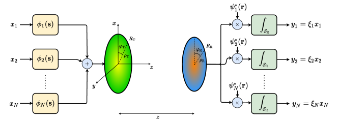
Figure 1: Schematic representation of communication modes between a couple of circular LISs in paraxial configuration and spaced of $z$.

Overall, the communication problem can be seen as a wireless interconnection of continuous apertures with finite extension in space, capable of generating and detecting the most suitable EM waveforms to maximize the achievable channel capacity. When only a finite number $N$ of basis functions are strongly coupled (i.e., with significant values of the corresponding $\xi_{n}$), the equivalent communication scheme which is obtained can be visualized as in Fig. 1. Remarkably, the adopted basis decomposition allows the definition of a system input-output representation in terms of $N$ parallel channels that is capacity-optimum, where $N$ identifies the available DoF for the specific communication system. Indeed, by associating the $N$ input data streams $\{x_{n}\}$ to the transmitting basis set $\{\phi_{n}(\textbf{s})\}$, $\textbf{s}\in S_{\text{T}}$, and neglecting the presence of noise, we are able to directly recover the transmitted data by performing the correlation of the received EM field with the corresponding basis functions $\{\psi_{n}(\mathbf{r})\}$, $\textbf{r}\in S_{\text{R}}$, thus obtaining $y_{n}=\xi_{n}x_{n}$, $n=1,\ldots,N$.

II-B Optimum Communication Modes with Circular LISs

Let us contemplate a paraxial geometry, which assumes that the transmitting and receiving LISs are parallel to each other and aligned at their centers. Considering circular antennas in paraxial conditions, the optimal wave functions describing the communication modes are the so-called circular prolate spheroidal functions (CPSFs) [46], extending the classical linear prolate spheroidal wave functions, which are instead solutions under paraxial conditions for rectangular antennas [7].

As illustrated in Fig. 1, let us consider two parallel, circular LISs in LOS. The coordinates $\rho_{\text{T}}$ and $\varphi_{\text{T}}$ in polar form represent a generic point on the transmitting LIS, while coordinates $\rho_{\text{R}}$ and $\varphi_{\text{R}}$ represent a generic point on the receiving LIS. The transmitting LIS antenna is located at a $z=0$, and the two LISs are separated by a distance of $z$. Moreover, the transmitting LIS has a radius $R_{\text{T}}$, and the receiving LIS has a radius $R_{\text{R}}$. The distance between two generic points on the transmitting and receiving LISs is denoted as

$$r=|\textbf{r}-\textbf{s}|=\sqrt{\rho_{\text{T}}^{2}+\rho_{\text{R}}^{2}-2\rho_{\text{T}}\rho_{\text{R}}\cos\left(\varphi_{\text{R}}-\varphi_{\text{T}}\right)+z^{2}}\,.$$ (8)

According to this geometry, the basis functions at the transmitting LIS are [46]

$$\phi_{n}(\rho_{\text{T}},\varphi_{\text{T}})=\frac{1}{\sqrt{2\pi R_{\text{T}}\rho_{\text{T}}}}f_{m,\ell}^{c}\left(\frac{\rho_{\text{T}}}{R_{\text{T}}}\right)e^{-\jmath\kappa\frac{\rho_{\text{T}}^{2}}{2z}}e^{\jmath\ell\varphi_{\text{T}}}$$ (9)

where $n=1,\ldots,N$ is the index spanning the elements in the set $\mathcal{S}=\{m,\ell\}$ corresponding to well-coupled communications modes, $\{f_{m,\ell}^{c}\}$ are the real-valued CPSFs that solve the band-limited Hankel-transform eigenvalue problem

$$\gamma_{m,\ell}^{c}f_{m,\ell}^{c}(x)=\int_{0}^{1}J_{\ell}\left(cxx^{\prime}\right)\sqrt{cxx^{\prime}}f_{m,\ell}^{c}\left(x^{\prime}\right)\text{d}x^{\prime}$$ (10)

in which $\gamma_{m,\ell}^{c}$ are the eigenvalues, $c=\frac{\kappa R_{\text{T}}R_{\text{R}}}{z}$ is the bandwidth parameter, $x^{\prime}=\frac{\rho_{\text{T}}}{R_{\text{T}}}$ and $x=\frac{\rho_{\text{R}}}{R_{\text{R}}}$. Correspondingly, at the receiving LIS side we have the basis functions [46]

$$\psi_{n}(\rho_{\text{R}},\varphi_{\text{R}})=\frac{1}{\sqrt{2\pi R_{\text{R}}\rho_{\text{R}}}}\frac{e^{\jmath\kappa z}}{\jmath^{\ell}}f_{m,\ell}^{c}\left(\frac{\rho_{\text{R}}}{R_{\text{R}}}\right)e^{\jmath\kappa\frac{\rho_{\text{R}}^{2}}{2z}}e^{\jmath\ell\varphi_{\text{R}}}\,.$$ (11)

According to [46], the coupling coefficient for the communication modes are

$$\xi_{n}=\gamma_{m,\ell}^{c}\sqrt{\frac{R_{\text{T}}R_{\text{R}}}{4\kappa z}}\,.$$ (12)

Due to the properties of eigenvalues $\gamma_{m,\ell}^{c}$ related to CPSFs, the number of communication modes (i.e., well-coupled modes) is given by [46]

$$N=\left(\frac{\pi R_{\text{T}}R_{\text{R}}}{\lambda z}\right)^{2}=\frac{S_{\text{T}}S_{\text{R}}}{\lambda^{2}z^{2}}$$ (13)

where the two areas of the LISs are given by $S_{\text{T}}=\pi R_{\text{T}}^{2}$ and $S_{\text{R}}=\pi R_{\text{R}}^{2}$. It is worth noting that (13) has the same form as classical results related to rectangular surfaces, as reported in [7]. However, this result is accurate only when $z$ is greater than the dimensions of the LISs.

Notably, both the transmitting and receiving basis functions $\phi_{n}(\rho_{\text{T}},\varphi_{\text{T}})$ and $\psi_{n}(\rho_{\text{R}},\varphi_{\text{R}})$ are separable in the radial and angular components, that is, they can be written respectively as

$$\phi_{n}(\rho_{\text{T}},\varphi_{\text{T}}) =\phi_{n}^{\rho}(\rho_{\text{T}})\,\phi_{n}^{\varphi}(\varphi_{\text{T}})$$ (14)

$$\psi_{n}(\rho_{\text{R}},\varphi_{\text{R}}) =\psi_{n}^{\rho}(\rho_{\text{R}})\,\psi_{n}^{\varphi}(\varphi_{\text{R}})\,.$$ (15)

III Orbital Angular Momentum

III-A General Definition

From the EM point of view, angular momentum is a vectorial characteristic that quantitatively defines the intrinsic rotation of the EM field [23]. While propagating in the axial direction indeed, a photons fashion can simultaneously rotate around its axis. Moreover, there are two different modalities of rotation, and each of them is associated with a specific component of the total angular momentum. Indeed, the total angular momentum can be computed as the sum of the spin angular momentum (SAM) and the orbital angular momentum (OAM). The SAM is related to the dynamic rotation of the electromagnetic field around its direction of propagation, and it is associated with the wave’s polarization [27]. OAM, instead, concerns the spatial distribution of the electromagnetic field and its rotation around the main beam axis [47].

From the physical point of view, the defining characteristic of EM waves that possess non-zero OAM is the emergence of wavefronts that deviate from the traditional far-field assumption of being parallel planes propagating in the axial direction. These wavefronts acquire a helical shape, twisted around the propagation direction. For this reason, OAM is frequently described as a vortex or with the notion of helical/twisted/screwed wavefront. Despite considering the scalar approximation as discussed in Sec. II, the particular helical structure of the wavefronts associated with OAM is typically represented in the wave equations by an exponential phase term, in the form of $e^{\jmath\ell\varphi}$, where $\ell\in\mathbb{Z}$ is referred to as the topological charge and $\varphi$ is the transverse azimuthal angle, defined as the angular position on a plane perpendicular to the propagation direction. In [27], it has been demonstrated that this characteristic represents a sufficient condition for the existence of OAM-carrying waves in a mostly paraxial propagation regime. Each vortex is thus characterized by an integer number $\ell$, whose magnitude represents the number of twists that a wavefront makes within a distance equal to the wavelength, and its sign determines the chirality or, equivalently, the direction of the twist. In fact, when $|\ell|>0$, the wavefront characterizing a specific topological charge has $|\ell|$ helices intertwined. Each of these states associated with a specific topological charge $\ell$ takes the name of OAM mode. The most interesting feature of OAM modes is their intrinsic orthogonality. In fact, we have

$$\int_{0}^{2\pi}e^{\jmath\ell_{j}\varphi}\left(e^{\jmath\ell_{k}\varphi}\right)^{*}\,\text{d}\varphi=\begin{cases}0&j\neq k\\ 2\pi&j=k\end{cases}$$ (16)

thus, in principle, beams exhibiting this characteristic could carry different data streams leading to spatial multiplexing capabilities.

Many types of beams carrying angular momentum have been investigated to impress the EM waves with the desired vorticose phase profile, among which LG beams are probably the most widely known [48]. LG beams are paraxial solutions of the wave equation in homogeneous media [49], and they are just an example of the plethora of existing waves able to carry OAM. Gaussian beams, Airy beams, and many others were subjects of research [50, 51], representing possible solutions to the problem of determining the best field distribution for OAM propagation. Interestingly, the common element between these kinds of beams is that all of them are reasonably able to transport OAM, and this characteristic is consistently described from the mathematical viewpoint through the exponential term $e^{\jmath\ell\varphi}$.

III-B OAM Modes and Communication Modes

The main difference concerning the definition of the OAM modes as, for example, LG beams, and communication modes as for the definition in Sec. II, is that for the former neither concepts nor references related to the specific transmitting/receiving antennas are given. Differently, communication modes, as identified by the couples of functions $(\phi_{n}(\textbf{s}),\psi_{n}(\textbf{r}))$, are strictly related to the geometry of the transmitting and receiving antennas. The fundamental dissimilarity between LG beams and communication modes arises from their distinct definitions. Indeed, LG beams are solutions of the wave equation in the absence of boundaries, i.e., with the source’s transverse dimensions approaching infinity. Conversely, communication modes in Sec. II are obtained by taking into account finite, well-defined antenna sizes. As a result, LG modes can be considered as approximate solutions of the actual propagating modes when the transmitting aperture is sufficiently large to generate the beams and the receiving aperture is adequate to capture them [46]. However, when boundaries corresponding to the finite transmitting/receiving antennas are considered, a limited number $N$ of well-coupled communication modes is obtained, and it holds that LG beams do not constitute proper solutions of (1) [52].

IV OAM-based Communications using LISs

The adoption of CPSFs as basis functions according to (9)-(11) leads to the highest number of communication modes. Unfortunately, such an approach results quite complex to be implemented, even in the paraxial scenario, for several reasons:

• The transmitting and receiving LISs should know exactly their mutual distance and sizes in order to shape the amplitude and phase profiles along the radial coordinates $\rho_{\text{T}}$ and $\rho_{\text{R}}$;

• A complex amplitude/phase profile must be drawn at the transmitting LIS side according to (9). Similarly, the received EM field must be properly weighted with a complex amplitude/phase profile according to (11). These operations require high flexibility at both the LISs.

In sight of this, there is an interest in designing ad-hoc transmitting and receiving basis functions of more straightforward implementation. To simplify the transmitting and receiving LISs architectures and exploit, at the same time, the multiplexing capabilities offered by the OAM helical wavefronts, the characteristic OAM exponential term could be leveraged to construct basis functions in the form of (14) that satisfy (1). In particular, we hereby propose to use the following orthonormal basis functions at the transmitting LIS side in the form of (14) where

$$\phi_{n}^{\rho}(\rho_{\text{T}}) =\frac{1}{R_{\text{T}}}\Pi_{R_{\text{T}}}(\rho_{\text{T}})$$ (17)

$$\phi_{n}^{\varphi}(\varphi_{\text{T}}) =\frac{1}{\sqrt{\pi}}e^{\jmath\ell_{n}\varphi_{\text{T}}}$$ (18)

with

$$\Pi_{a}(\beta)=\begin{cases}1&\beta\in(0,a)\\ 0&\text{otherwise}\end{cases}\,$$ (19)

being the rectangular function, which in our specific case identifies a disk of radius $R_{\text{T}}$, and

$$\ell_{n}=\begin{cases}-\frac{n-1}{2}&\mod(n,2)=1\\ \frac{n}{2}&\mod(n,2)=0\end{cases}$$ (20)

for $n=1,\ldots,N$. Consequently, $\ell_{n}=0,+1,-1,+2,-2,\ldots,(N-1)/2$, assuming $N$ odd. The transmitting functions proposed in (17)-(18) are normalized such that they exhibit unitary energy, i.e.,

$$\int_{0}^{R_{\text{T}}}\int_{0}^{2\pi}\phi_{n}(\rho_{\text{T}},\varphi_{\text{T}})\phi_{m}^{*}(\rho_{\text{T}},\varphi_{\text{T}})\rho_{\text{T}}\,\text{d}\varphi_{\text{T}}\,\text{d}\rho_{\text{T}}=\delta_{nm}$$ (21)

being $\delta_{nm}$ the Kronecker delta, hence ensuring that the overall transmitted energy is equal to $E_{\mathrm{t}}=N$.

These bases can be viewed as the extension to a circular surface of the typical phase tapering profiles required to generate OAM waves with UCAs. In fact, a well-known technique for obtaining the helical wavefronts consists of feeding a circular array of $N_{\text{TX}}$ elements equally spaced over a ring, with a successive phase delay $\Delta=2\ell\pi/N_{\text{TX}}$ such that, after a complete turn, the phase is incremented of a multiple integer $\ell$ of $2\pi$ (i.e., phase varying linearly with the azimuthal angle) [53]. Notably, functions (17)-(18) could be used to realize spatial multiplexing by requiring phase-tapering only at the transmitter, thereby significantly simplifying the implementation of the LIS. These functions do not form a complete basis set, unlike the optimum solutions, hence a performance degradation in terms of DoF is expected, as it will be investigated in the following. It is important to note that when $n=1$ (or, equivalently, $\ell_{n}=0$), the resulting beam is the same as a uniform circular aperture, while the subsequent modes are degenerate. This means that the same coupling is obtained for adjacent modes (e.g., for $n=2$ and $n=3$, which correspond to topological charges with the same absolute values but opposite chirality).

When the basis function $\phi_{n}(\rho_{\text{T}},\varphi_{\text{T}})$ specified in (17)-(18) is employed at the transmitting antenna, the resulting field at a distance $z$ as described by (2) can be computed as

$$\psi_{n}(\rho_{\text{R}},\varphi_{\text{R}})= \frac{1}{R_{\text{T}}\sqrt{\pi}}\int_{0}^{R_{\text{T}}}\int_{0}^{2\pi}e^{\jmath\ell_{n}\varphi_{T}}\frac{e^{-\jmath\kappa r}}{4\pi r}\rho_{\text{T}}\,\text{d}\varphi_{\text{T}}\,\text{d}\rho_{\text{T}}$$ (22)

Particularly, when waves propagate within the Fresnel zone, which allows for multiple communication modes to be established, the variable $r$ in the numerator of (22) can be approximated with [54]

$$r\approx z+\frac{\rho_{\text{T}}^{2}}{2z}+\frac{\rho_{\text{R}}^{2}}{2z}-\frac{\rho_{\text{T}}\rho_{\text{R}}\cos(\varphi_{\text{R}}-\varphi_{\text{T}})}{z}$$ (23)

while in the denominator of (22) we consider $r\approx z$. This conventional Fresnel approximation leads to the expression of the received EM field as

$$\psi_{n}(\rho_{\text{R}},\varphi_{\text{R}}) \simeq\frac{1}{4\pi zR_{\text{T}}\sqrt{\pi}}e^{-\jmath\kappa\frac{\rho_{\text{R}}^{2}}{2z}}e^{-\jmath\kappa z}\int_{0}^{R_{\text{T}}}\int_{0}^{2\pi}e^{\jmath\ell_{n}\varphi_{\text{T}}}e^{-\jmath\kappa\frac{\rho_{\text{T}}^{2}}{2z}}e^{\jmath\kappa\frac{\rho_{\text{R}}\rho_{\text{T}}\cos{(\varphi_{\text{R}}-\varphi_{\text{T}})}}{z}}\rho_{\text{T}}\,\text{d}\varphi_{\text{T}}\,\text{d}\rho_{\text{T}}$$

$$=\frac{(-1)^{\ell_{n}}}{2z\sqrt{2\pi R_{\text{T}}}}e^{-\jmath\kappa\frac{\rho_{\text{R}}^{2}}{2z}}e^{-\jmath\kappa z}e^{\jmath\ell_{n}\varphi_{\text{R}}}\int_{0}^{R_{\text{T}}}\rho_{\text{T}}e^{-\jmath\kappa\frac{\rho_{\text{T}}^{2}}{2z}}J_{\ell_{n}}\left(\frac{\kappa\rho_{\text{R}}\rho_{\text{T}}}{z}\right)\,\text{d}\rho_{\text{T}}\,.$$ (24)

It can be noticed from (22) that the exponential term $e^{\jmath\ell\varphi_{\text{R}}}$ identifying OAM is also present in the received EM field expression. This shows that OAM wavefronts propagate in free space with no changes and irrespectively of the selected transmitting profile along the radial direction, thus demonstrating how orthogonality is preserved at the receiver although modifying the OAM beams’ shapes. In the remainder, we dub as OAM mode each EM field component $\psi_{n}(\rho_{\text{R}},\varphi_{\text{R}})$ generated by the basis function in (17)-(18).

IV-A Focused OAM

When considering the OAM modes at the receiving LIS according to the discussion thus far, it can be noticed from the analytical expression in (IV) that, as the topological charge increases, higher-order modes exhibit maximum values at increasingly larger values of $\rho_{\text{R}}$, which is a characteristic of the Bessel functions. Indeed, it is a widely acknowledged fact that the divergence of the OAM-carrying beams increases with the topological charge [55]. Therefore, a large receiving LIS is required to collect most of the beam and obtain a significant coupling intensity. Moreover, the beam-widening effect is more pronounced when operating in the near field, as the diffraction pattern of an aperture is inherently larger than that observed in the far field. This is a consequence of the convolution with a quadratic-phase term, as reported in (IV). A widely adopted method for restricting the angular spread of a beam in the near field is through the use of focusing techniques [56]. This approach consists in adjusting the phase of a radiating source so that it compensates for the propagation delay towards a specific point (the focal point), where all the EM field contributions add coherently, thus enhancing the EM field intensity in a limited-area region. Achieving this desired outcome, by utilizing the functions presented in (17)-(18), requires a modification of the transmitting phase profile $\phi_{n}(\rho_{\text{T}},\varphi_{\text{T}})$ along the radial coordinate $\rho_{\text{T}}$, such that the phase converges at the focal point. In the context of paraxial geometry, where the focal point is located at the center of the receiving LIS at a distance $z$, this can be accomplished by adopting

$$\phi_{n}^{\rho}(\rho_{\text{T}})\!=\!\frac{\Pi_{R_{\text{T}}}(\rho_{\text{T}})}{R_{\text{T}}}\left.e^{\jmath\kappa r}\right|_{\rho_{\text{R}}=0}\!\approx\!\frac{\Pi_{R_{\text{T}}}(\rho_{\text{T}})}{R_{\text{T}}}e^{\jmath\kappa z\left(1+\frac{\rho_{\text{T}}^{2}}{2z^{2}}\right)}$$ (25)

where the right-hand approximation is derived from the Fresnel approximation outlined in (23).

From a practical perspective, focusing can be achieved by utilizing the phase profile $\phi_{n}^{\rho}(\rho_{\text{T}})=\Pi_{R_{\text{T}}}(\rho_{\text{T}})\exp{(\jmath\kappa{\rho_{\text{T}}^{2}}/{2z})}/R_{\text{T}}$, as the inclusion of a constant phase term does not affect the focusing behavior. As the separability described in (14) highlights, the application of the phase profile along the transverse radial coordinate $\rho_{\text{T}}$ does not alter the helical phase front, thus maintaining orthogonality at both the transmitter and receiver sides. Indeed, any variation of the phase profile along the radial coordinate $\rho_{\text{T}}$ does not entail any loss in terms of beams’ separation. A limitation of this method is that the distance between the antennas must be known at the transmitting LIS side in order to properly focus the EM field. Nevertheless, this strategy requires phase-tapering only, thus leading to a simple implementation. As a consequence, the overall system complexity in the presence of focusing is in any case reduced with respect to the optimum strategy in Sec. III.B.

When the phase profile (25) is adopted, at the receiving LIS side the resulting EM field can be expressed as

$$\psi_{n}(\rho_{\text{R}},\varphi_{\text{R}}) \simeq\frac{1}{4\pi zR_{\text{T}}\sqrt{\pi}}e^{-\jmath\kappa\frac{\rho_{\text{R}}^{2}}{2z}}\int_{0}^{R_{\text{T}}}\int_{0}^{2\pi}e^{\jmath\ell_{n}\varphi_{\text{T}}}e^{\jmath\kappa\frac{\rho_{\text{R}}\rho_{\text{T}}\cos{(\varphi_{\text{R}}-\varphi_{\text{T}})}}{z}}\rho_{\text{T}}\,\text{d}\varphi_{\text{T}}\,\text{d}\rho_{\text{T}}$$

$$=\frac{(-1)^{\ell_{n}}}{2zR_{\text{T}}\sqrt{\pi}}e^{-\jmath\kappa\frac{\rho_{\text{R}}^{2}}{2z}}e^{\jmath\ell_{n}\varphi_{\text{R}}}\int_{0}^{R_{\text{T}}}\rho_{\text{T}}J_{\ell_{n}}\left(\frac{\kappa\rho_{\text{R}}\rho_{\text{T}}}{z}\right)\,\text{d}\rho_{\text{T}}\,.$$ (26)

Interestingly, the expression in (IV-A) corresponds to the beam that would be obtained with the far-field (Fraunhofer) approximation, even though the field is being observed within the Fresnel zone of the transmitting LIS [45, 57]. Indeed, by focusing along $\rho_{\text{T}}$, the quadratic phase term responsible for the diffraction effects typical of the Fresnel zone is compensated, hence resulting in a more concentrated beam at the focal point. Notice that, when $\ell_{n}=0$ (i.e., $n=1$), we have

$$\psi_{1}(\rho_{\text{R}},\varphi_{\text{R}})= \frac{1}{2zR_{\text{T}}\sqrt{\pi}}e^{-\jmath\kappa\frac{\rho_{\text{R}}^{2}}{2z}}\int_{0}^{R_{\text{T}}}\rho_{\text{T}}J_{0}\left(\frac{\kappa\rho_{\text{R}}\rho_{\text{T}}}{z}\right)\,\text{d}\rho_{\text{T}}$$

$$= \frac{1}{2z\sqrt{\pi}}e^{-\jmath\kappa\frac{\rho_{\text{R}}^{2}}{2z}}J_{1}\left(\frac{\kappa\rho_{\text{R}}R_{\text{T}}}{z}\right)\,.$$ (27)

The intensity profile corresponding to (IV-A) is the classical far-field pattern of a circular aperture antenna (i.e., the Airy disk [54]). Remarkably, higher topological charges produce a beam divergence partially compensated by focusing, as it will be investigated in the following numerical example.

IV-B Numerical Example

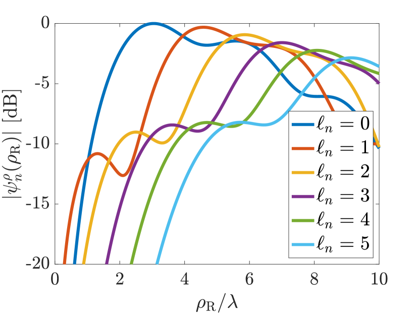
(a) Unfocused case

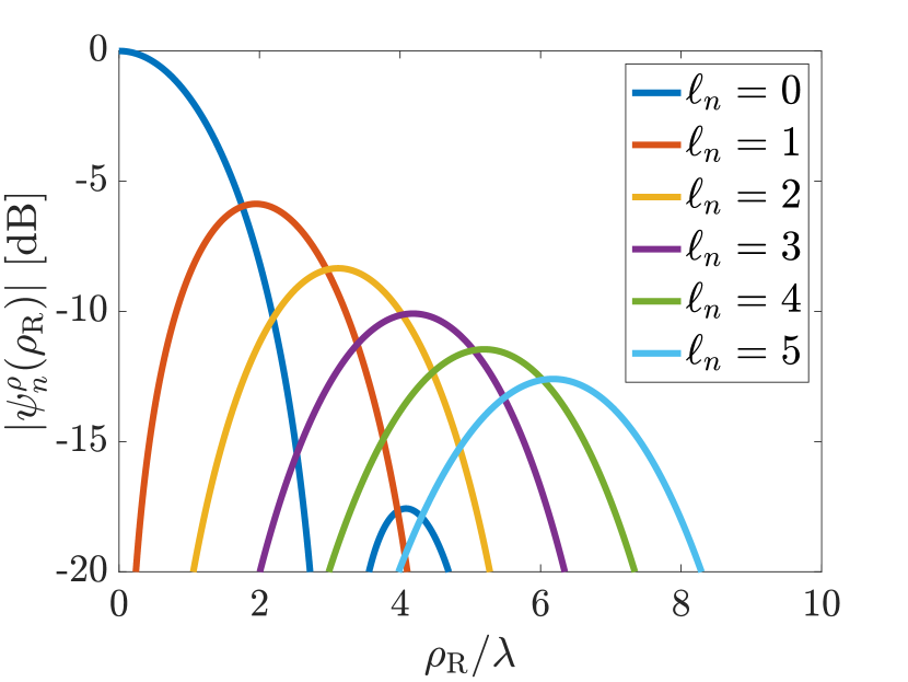
(b) Focused case

Figure 2: Received EM field along the radial coordinate as a function of the ratio $\rho_{\text{R}}/\lambda$ for different topological charges $\ell_{n}$ (a) in the absence and (b) in the presence of a focusing transmitting LIS (normalized to $\operatorname{max}\{|\psi_{1}^{\rho}(\rho_{\mathrm{R}})|\})$.

As an example, let us consider two parallel, circular LISs placed at a distance $z=D\lambda$. The transmitting LIS has a radius $R_{\text{T}}=T\lambda$, while the receiving LIS has a radius $R_{\text{R}}=R\lambda$. Fig. 2(a) illustrates the normalized amplitude of the received electric field’s radial component $\psi_{n}^{\rho}(\rho_{\text{R}})$, where $\psi_{n}(\rho_{\text{R}},\varphi_{\text{R}})=\psi_{n}^{\varphi}(\varphi_{\text{R}})\psi_{n}^{\rho}(\rho_{\text{R}})$ and $\psi_{n}^{\varphi}(\varphi_{\text{R}})=e^{\jmath\ell_{n}\varphi_{\text{R}}}$, as a function of the ratio $\rho_{\text{R}}/\lambda$ for the case $R=T=10$ and $D=50$. It can be observed that the beam divergence increases with higher values of the topological charge $\ell_{n}$. Furthermore, the beam widening effect, which is a characteristic of the received EM field within the Fresnel zone, is also visible. In fact, within the chosen numerical setup, the boundary between the near-field and far-field (i.e., the Fraunhofer distance $d_{\mathrm{ff}}$) is in our case [54]

$$d_{\mathrm{ff}}=\frac{8R_{\text{T}}^{2}}{\lambda}$$ (28)

and it can be written in terms of a multiple of the wavelength $\lambda$ as $D_{\mathrm{ff}}=d_{\mathrm{ff}}/\lambda=8T^{2}$. It should be noted that $D_{\mathrm{ff}}>D$ in the suggested numerical example.

In contrast, when a focusing transmitting LIS side is adopted according to (25) with the same system configuration, the amplitude of the radial component of the normalized received electric field is that as reported in Fig. 2(b). The focusing effect is clearly visible, producing much more concentrated beams, thus maximizing the energy collected by the receiving LIS. As it is possible to notice from the figure, each beam is characterized by a different level of divergence, increasing with the mode order. Additional examples of the amplitude and phase profiles obtained both at the transmitting and receiving LIS for different topological charges are reported in Appendix A, either in the presence or in the absence of focusing at the transmitting LIS.

V Detection Strategies

When $N$ data streams are transmitted simultaneously to carry the symbols ${\bf x}=\{x_{1},\ldots,x_{N}\}$, i.e., spatially multiplexed according to the basis functions $\phi_{n}(\rho_{\text{R}},\varphi_{\text{R}})$ in (17)-(18), the information-carrying EM field resulting from the modes’ superposition at a distance $z$ (i.e., at the receiving LIS) is given by

$$y(\rho_{\text{R}},\varphi_{\text{R}})=\psi(\rho_{\text{R}},\varphi_{\text{R}})+n(\rho_{\text{R}},\varphi_{\text{R}})=\sum_{n=1}^{N}x_{n}\psi_{n}(\rho_{\text{R}},\varphi_{\text{R}})+n(\rho_{\text{R}},\varphi_{\text{R}})$$ (29)

where $y(\rho_{\text{R}},\varphi_{\text{R}})$ identifies the overall received EM field, the first addend represents the useful EM field carrying the data, and $n(\rho_{\text{R}},\varphi_{\text{R}})$ denotes a noise field affecting the OAM-based system. In the absence of further assumptions (e.g., regarding electromagnetic interference [58]), the noise field, when expressed in Cartesian coordinates, is considered as additive white Gaussian noise (AWGN) within the useful signal’s spatial bandwidth, as further characterized in Appendix B.

The total energy received per symbol is

$$E_{\mathrm{s}}=\int_{0}^{R_{\text{R}}}\int_{0}^{2\pi}\left|\psi(\rho_{\text{R}},\varphi_{\text{R}})\right|^{2}\rho_{\text{R}}\,\text{d}\varphi_{\text{R}}\,\text{d}\rho_{\text{R}}$$ (30)

so that we define the signal-to-noise ratio (SNR) as $\mathsf{SNR}=E_{\mathrm{s}}/N_{0}$. Consequently, the SNR associated with the $n$-th OAM mode can be written as

$$\mathsf{SNR}_{n}=\mathsf{SNR}\,\frac{E_{n}}{E_{\mathrm{s}}}$$ (31)

being $E_{n}=\int_{0}^{2\pi}\int_{0}^{\rho_{\text{R}}}\left|\psi_{n}(\rho_{\text{R}},\varphi_{\text{R}})\right|^{2}\rho_{\text{R}}\,\text{d}\varphi_{\text{R}}\,\text{d}\rho_{\text{R}}$ the energy of the $n$-th received OAM mode. In addition, we define the parameter $\eta$ as the ratio between the overall received energy and the transmitted energy as

$$\eta =\frac{E_{\mathrm{s}}}{\int_{0}^{R_{\text{T}}}\int_{0}^{2\pi}\left|\sum_{n=1}^{N}\phi_{n}(\rho_{\text{T}},\varphi_{\text{T}})\right|^{2}\rho_{\text{T}}\,\text{d}\varphi_{\text{T}}\,\text{d}\rho_{\text{T}}}=\frac{E_{\mathrm{s}}}{E_{\mathrm{t}}}\,.$$ (32)

This quantity is conceptually equivalent to the inverse of the free-space path loss (i.e., path gain), and it will be further discussed in Sec. VI.

V-A OAM Demultiplexing

At the receiving LIS side, the overall EM field $y(\rho_{\text{R}},\varphi_{\text{R}})$ is processed to extract the information data ${\bf x}$. Remarkably, thanks to the helical wavefront propagating with no changes along the azimuthal coordinate, a correlation at the receiving LIS side with a conjugate factor $e^{-\jmath\ell_{n}\varphi_{\text{R}}}$ enables to isolate the $n$-th contribution $\psi_{n}(\rho_{\text{R}},\varphi_{\text{R}})$ from the total received field in (29), thus performing OAM modes’ demultiplexing. Formally, it holds

$$y_{n}(\rho_{\text{R}}) =\int_{0}^{2\pi}y(\rho_{\text{R}},\varphi_{\text{R}})e^{-\jmath\ell_{n}\varphi_{\text{R}}}\,\text{d}\varphi_{\text{R}}$$

$$=\int_{0}^{2\pi}\sum_{n=1}^{N}x_{n}\psi_{n}(\rho_{\text{R}},\varphi_{\text{R}})e^{-\jmath\ell_{n}\varphi_{\text{R}}}\,\text{d}\varphi_{\text{R}}+\int_{0}^{2\pi}n(\rho_{\text{R}},\varphi_{\text{R}})e^{-\jmath\ell_{n}\varphi_{\text{R}}}\,\text{d}\varphi_{\text{R}}$$

$$=x_{n}\psi_{n}^{\rho}(\rho_{\text{R}})+n_{n}(\rho_{\text{R}})\,$$ (33)

where

$$\psi_{n}^{\rho}(\rho_{\text{R}})=\frac{(-1)^{\ell_{n}}}{2zR_{\text{T}}\sqrt{\pi}}e^{-\jmath\kappa\frac{\rho_{\text{R}}^{2}}{2z}}e^{-\jmath\kappa z}\int_{0}^{R_{\text{T}}}\rho_{\text{T}}e^{-\jmath\kappa\frac{\rho_{\text{T}}^{2}}{2z}}J_{\ell_{n}}\left(\frac{\kappa\rho_{\text{R}}\rho_{\text{T}}}{z}\right)\,\text{d}\rho_{\text{T}}\,$$ (34)

when focusing is not performed the transmitting LIS side and

$$\psi_{n}^{\rho}(\rho_{\text{R}})=\frac{(-1)^{\ell_{n}}}{2zR_{\text{T}}\sqrt{\pi}}e^{-\jmath\kappa\frac{\rho_{\text{R}}^{2}}{2z}}e^{-\jmath\kappa z}\int_{0}^{R_{\text{T}}}\rho_{\text{T}}J_{\ell_{n}}\left(\frac{\kappa\rho_{\text{R}}\rho_{\text{T}}}{z}\right)\,\text{d}\rho_{\text{T}}\,$$ (35)

when focusing is instead employed at the transmitting LIS. The function $n_{n}(\rho_{\text{R}})$ denotes the radial noise portion after demultiplexing affecting the $n$-th OAM mode that is being detected.

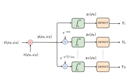
Figure 3: Equivalent block diagram of the OAM modes demultiplexing.

Then, different approaches can be employed to build a scalar decision variable $Y_{n}$ by processing the signal over the radial component $\rho_{\text{R}}$ of the LIS, thus detecting the transmitted symbol $x_{n}$ from the $n$-th EM field component. An overview of the equivalent receiver block diagram performing OAM demultiplexing is reported in Fig. 3. In the following, we illustrate three different detection strategies corresponding to different levels of implementation complexity and performance.

V-B Matched Filter

The optimum strategy for maximizing the energy at the $n$-th branch of the receiver is that of performing matched filtering, i.e., computing the correlation also along the radial coordinate $\rho_{\text{R}}$ using a template function $f_{n}(\rho_{\text{R}})$ matched to (34) or (35), i.e., $f_{n}(\rho_{\text{R}})=\psi_{n}^{\rho}(\rho_{\text{R}})$. Notably, due to the assumption of spatially white noise and the adoption of a polar reference system, the correlation-based reception scheme requires the introduction of the determinant of the Jacobian matrix associated with the Cartesian to polar coordinates’ transformation as in (21)-(22), that is, $\rho_{\text{R}}$. Thus, the decision variable $Y_{n}^{\text{(MF)}}$ used for signal demodulation at the $n$-th branch is

$$Y_{n}^{\text{(MF)}} =\int_{0}^{R_{\text{R}}}y_{n}(\rho_{\text{R}})\,f_{n}^{*}(\rho_{\text{R}})\rho_{\text{R}}\,\text{d}\rho_{\text{R}}$$

$$=x_{n}\int_{0}^{R_{\text{R}}}\left|\psi_{n}^{\rho}(\rho_{\text{R}})\right|^{2}\rho_{\text{R}}\,\text{d}\rho_{\text{R}}+\int_{0}^{R_{\text{R}}}n_{n}(\rho_{\text{R}})f_{n}^{*}(\rho_{\text{R}})\rho_{\text{R}}\,\text{d}\rho_{\text{R}}$$

$$=x_{n}h_{n}^{\text{(MF)}}+w_{n}$$ (36)

where $h_{n}^{\text{(MF)}}$ denotes the $n$-th channel coefficient describing the effects of OAM LOS propagation. Precisely, it holds $h_{n}^{\text{(MF)}}=E_{n}$, with

$$E_{n}=\frac{1}{4\pi z^{2}R_{\text{T}}^{2}}\int_{0}^{R_{\text{R}}}\!\left|\int_{0}^{R_{\text{T}}}\rho_{\text{T}}e^{-\jmath\kappa\frac{\rho_{\text{T}}^{2}}{2z}}J_{\ell_{n}}\left(\frac{\kappa\rho_{\text{R}}\rho_{\text{T}}}{z}\right)\text{d}\rho_{\text{T}}\right|^{2}\,\rho_{\text{R}}\text{d}\rho_{\text{R}}$$ (37)

being the received energy related to the $n$-th OAM mode when focusing is not performed by the transmitting LIS, and

$$E_{n}=\frac{1}{4\pi z^{2}R_{\text{T}}^{2}}\int_{0}^{R_{\text{R}}}\left|\int_{0}^{R_{\text{T}}}\rho_{\text{T}}J_{\ell_{n}}\left(\frac{\kappa\rho_{\text{R}}\rho_{\text{T}}}{z}\right)\text{d}\rho_{\text{T}}\right|^{2}\rho_{\text{R}}\,\text{d}\rho_{\text{R}}$$ (38)

when accounting for the presence of focusing instead. In addition, $w_{n}$ denotes the noise component affecting the decision variable at the output of the $n$-th correlation-based device. We have that, $w_{n}\sim\mathcal{CN}(0,\,\sigma_{w,\text{MF}}^{2})$, $n=1,2,\ldots,N$, are independent, identically distributed (i.i.d.) circularly-symmetric complex Gaussian random variables, whose variance is derived in Appendix B.

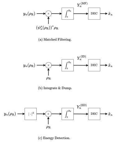
Figure 4: Proposed radial processing schemes for symbol detection after OAM modes demultiplexing.

Unfortunately, such a strategy, whose equivalent processing scheme is reported in Fig. 4a, despite maximizing the SNR at its output, requires high flexibility at the receiving LIS side. In fact:

• The spatial correlation with a complex amplitude/phase pattern must be performed;

• The distance between the transmitter and receiver, as well the transmitting LIS’s size, must be known at the receiver side to build the template function $f_{n}(\rho_{\text{R}})$.

V-C Integrate & Dump

Considering that the total received field comprises a set of well-defined beams, especially in the focused case (as in Fig. 2(b)), a lower-complexity detection scheme could be achieved by means of a simple integrate & dump (ID) approach (i.e., accumulation over the radial coordinate $\rho_{\text{R}}$), thus obviating the need for point-wise processing along $\rho_{\text{R}}$ involving a complex amplitude and phase spatial correlation.

Specifically, we have

$$Y_{n}^{\text{(ID)}} =\int_{0}^{R_{\text{R}}}y_{n}(\rho_{\text{R}})\rho_{\text{R}}\,\text{d}\rho_{\text{R}}$$

$$=x_{n}\int_{0}^{R_{\text{R}}}\psi_{n}^{\rho}(\rho_{\text{R}})\rho_{\text{R}}\,\text{d}\rho_{\text{R}}+\int_{0}^{R_{\text{R}}}n_{n}(\rho_{\text{R}})\rho_{\text{R}}\,\text{d}\rho_{\text{R}}$$

$$=x_{n}h_{n}^{\text{(ID)}}+w_{n}^{\text{(ID)}}$$ (39)

with $h_{n}^{\text{(ID)}}$ being the complex channel coefficent, and $w_{n}^{\text{(ID)}}\sim\mathcal{CN}(0,\,\sigma_{w,\text{ID}}^{2})$, $n=1,\ldots,N$, being the Gaussian noise variables with variance $\sigma_{w,\text{ID}}^{2}$, derived in Appendix B. This strategy corresponds to assuming $f_{n}(\rho_{\text{R}})=\Pi_{R_{\text{R}}}(\rho_{\text{R}})$, hence integrating on the totality of the receiving radial dimension. The equivalent processing scheme is reported in Fig. 4b. It is worth noticing that, in this case, differently from the matched filter (MF) strategy, the lack of the square module operation in (V-C), which is instead present in (V-B), makes the complex output variable $Y_{n}^{\text{(ID)}}$ dependent in its sign on the positive/negative result of the integral of the radial component $\psi_{n}(\rho_{\text{R}})$. Thus, the final decision criterion must account for this. Moreover, channel equalization is required to compensate for the phase term in the decision variable.

V-D Energy Detection

In order to further simplify the receiver structure, a partially non-coherent scheme can be considered, by collecting the energy along the radial component $\rho_{\text{R}}$ exploiting a square-law device, thus leading to an energy detector (ED) scheme. After demultiplexing the $n$-th OAM mode as previously described, the square module is then computed and, subsequently, the integration in the radial direction is performed to obtain the scalar decision variable $Y_{n}^{\text{(ED)}}$, i.e.,

$$Y_{n}^{\text{(ED)}} =\int_{0}^{R_{\text{R}}}\left|y_{n}(\rho_{\text{R}})\right|^{2}\rho_{\text{R}}\,\text{d}\rho_{\text{R}}$$

$$=\int_{0}^{R_{\text{R}}}\left|x_{n}\psi_{n}^{\rho}(\rho_{\text{R}})+n_{n}(\rho_{\text{R}})\right|^{2}\rho_{\text{R}}\,\text{d}\rho_{\text{R}}.$$ (40)

The equivalent processing scheme is reported in Fig. 4c. Conversely to the other detection strategies, energy detection cannot be realized with the general communication scheme of Fig. 1, since integration over the angular coordinate $\varphi_{\text{R}}$ only is required and, afterward, non-linear processing along the radial coordinate $\rho_{\text{R}}$ is performed.

Differently from the MF and the ID schemes, this detection strategy introduces some additional constraints to be considered. For instance, due to the presence of the square law device in the reception scheme, any information regarding the signal’s phase is lost, thus requiring non-coherent modulation schemes such as on-off keying (OOK), as we will assume in the following. This particular choice leads to two possible outcomes: a first case in which the decision variable $Y_{n}^{\text{(ED)}}$ is composed of the noise energy only, and a second one in which $Y_{n}^{\text{(ED)}}$ comprises both the transmitted signal and the noise energies. The final symbol’s decision can be performed by comparing the energy level measured at the radial integration block’s output, i.e., $Y_{n}^{\text{(ED)}}$, with an appropriate threshold value. Therefore, the decision criterion becomes

$$\hat{x}_{n}=\begin{cases}+1,&Y_{n}^{\text{(ED)}}\geq\zeta_{n}\\ 0,&Y_{n}^{\text{(ED)}}<\zeta_{n}\end{cases}$$ (41)

where $\zeta_{n}$ identifies the decision threshold that has been suitably defined for the $n$-th OAM mode. In Sec. VI, appropriate threshold values for $\zeta_{n}$, $n=1,\ldots,N$, will be numerically evaluated for a given SNR at the receiver.

V-E Smart Integration

In Sec. V-A, it has emerged how, after performing a first correlation of the total received EM field with the conjugate phase factor $e^{-\jmath\ell_{n}\varphi_{\text{R}}}$ of the mode of interest to be demultiplexed, integration in the radial variable $\rho_{\text{R}}$ needs to be performed. When the MF scheme is employed, this operation results in maximizing the SNR at the receiving LIS, being the selected receiver template functions matched to the received waveforms. However, when the ID or ED strategies are contemplated, the absence of a radial processing matched to the received signal $\psi_{n}^{\rho}(\rho_{\text{R}})$ might lead to a subtle deterioration in performance. This is because when integrating along the totality of the radial domain, i.e., $\rho_{\text{R}}\in[0,R_{\text{R}}]$, a consistent amount of noise is accumulated, which comes from those locations on the receiving LIS where the radial signal component $\psi_{n}^{\rho}(\rho_{\text{R}})$ has negligible values, as shown in Figs. 2(b). Indeed, both with focused or unfocused beams, the received field amplitude tends to be concentrated on a given radial interval, hence rapidly vanishing outside of it.

To counteract this phenomenon, a viable solution is that of computing the integral only where the received EM field has a significant intensity. This operation has been dubbed as smart integration since we assume to have an intelligent receiving device that, given the knowledge of the OAM order that has been demultiplexed, can identify a suitable domain on which to perform the integration operation. The procedure is similar to the problem of integration time determination for non-coherent receivers, for which several solutions have been proposed in the literature [59, 60, 61]. Examples will be given in the numerical results of Sec. VI.

VI Numerical Study

VI-A Degrees of Freedom

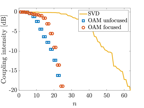
Figure 5: Coupling intensity for the unfocused and focused OAM modes in comparison with the coupling intensity of optimum communication modes (SVD).

To evaluate the effectiveness of the OAM approach, we compare the coupling intensity obtained with OAM modes to the coupling intensity obtained from optimum communication modes (i.e., the intensity of the singular values $\xi_{n}$ as from the optimum basis sets). The optimal bases are obtained by discretizing the transmitting and receiving LISs and computing the singular value decomposition (SVD) of the Green function (3) between the surfaces. In Fig. 5, the behavior of singular values is reported for the configuration $R=T=10$ and $D=50$, with $\lambda=0.1\,$m. It can be seen that they are almost constant, then drop quickly after a specific value. The number of effective communication modes $N$, i.e., the DoF, can be defined as the number of singular values of intensity no smaller than a certain value with respect to the largest one. The coupling intensity of the OAM modes corresponds to the normalized values $E_{n}/E_{1}$, being the denominator coincident with the energy of the fundamental mode $n=1$ (i.e., $\ell_{n}=0$). As anticipated, OAM-based modes are degenerate, hence the same coupling is obtained for two consecutive indexes $n$, except for the case $n=1$. Due to the presence of beam divergence, OAM modes coupling falls off quite rapidly compared to the optimal case. However, it can be noticed how beneficial the adoption of focusing techniques is in terms of coupling strength. In this setup, by fixing a threshold to $-5\,\text{dB}$ from the best-connected communication mode, about 40 communication modes are obtained with SVD; differently, only 10 can be exploited with OAM and about 18 with OAM when performing focusing at the transmitting LIS. Therefore, it is evident that the number of parallel channels is lower than that corresponding to the optimum strategy. However, system complexity is significantly reduced. In particular, the coupling intensity obtained for focused OAM-based communication modes with low topological charge is anyhow acceptable, so this could be reasonably exploited for enhancing the link capacity with small additional complexity in terms of hardware implementation. A detailed analysis of the trade-off between ease of deployment and the required level of system knowledge will be thoroughly provided in Sec. VI-C. In Fig. 6(a), the number of modes $N$ is depicted as a function of the distance parameter $D$ for the scenario of $R=T=10$. For comparison, the number of communication modes obtained from (13) is also illustrated. In particular, it is convenient to rewrite (13) as a function of the normalized quantities considered in the numerical results, which gives

$$N=\frac{\pi^{2}R^{2}T^{2}}{D^{2}}\,$$ (42)

and which depends only on geometrical quantities reported to the wavelength. Furthermore, the number of modes obtained by considering the singular values from the SVD is also illustrated. In all cases, a threshold of $-5\,\text{dB}$ is applied to determine the number of well-coupled modes. As expected, regardless of the adopted strategy, the number of modes diminishes rapidly for increasing distance, reaching unity as the far-field limit is approached. The number of modes corresponding to significant singular values from the SVD is accurately predicted by (42). While the use of focused OAM results in a greater number of well-coupled modes, both the focused and unfocused OAM transmissions have inferior performance compared to optimum communication modes when the distance is small. However, when the geometric setting does not allow for a large number of modes (e.g., for larger distances), OAM can be used as a viable solution to exploit channel spatial multiplexing, with limited additional complexity and without the need to perform SVD.

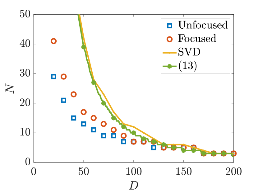
(a) Antennas of the same size ($R=T=10$).

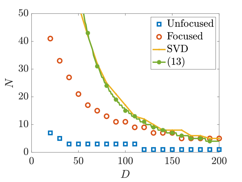
(b) Downlink case ($R=5,T=25$).

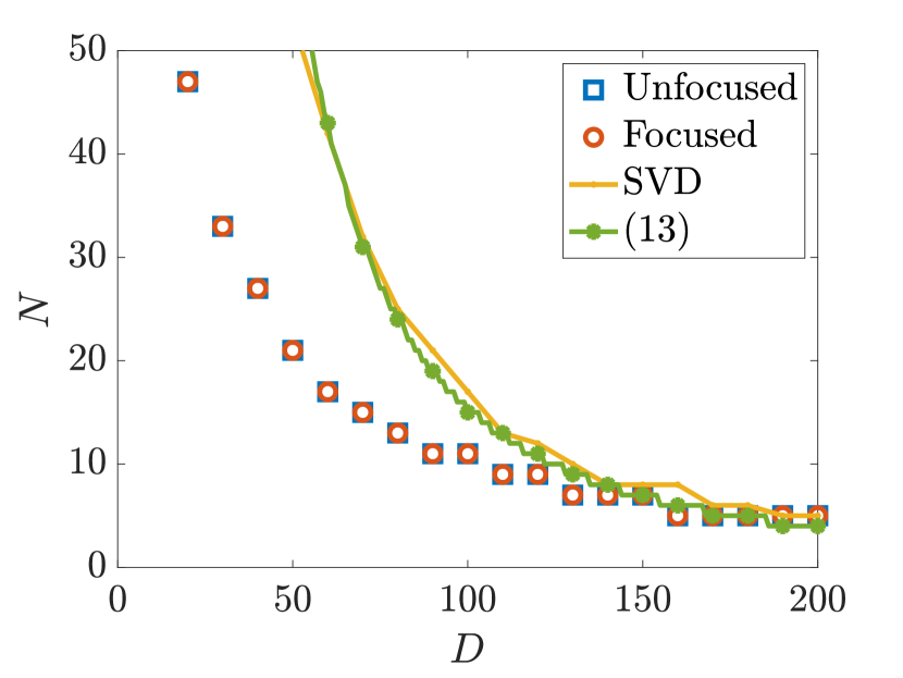
(c) Uplink case ($R=25,T=5$).

Figure 6: Number of OAM modes as a function of the link distance $D$ (multiples of $\lambda$).

Furthermore, the following plots show what happens when the sizes of the LISs greatly differ. In particular, in Fig. 6(b) LIS antennas with $R=5$ and $T=25$ are considered. Since the transmitting antenna is much larger than the receiving one, we refer to this scenario as the downlink case. Thanks to the large dimensions of the transmitting LIS, a high focusing gain can be obtained, thus drastically increasing the number of well-coupled OAM-based channels. Differently, if focusing is not adopted in this downlink case, the detrimental effect of beam divergence, exasperated by the large transmitting aperture, makes OAM-based strategies quite ineffective. The opposite case, corresponding to $R=25$ and $T=5$ (i.e., uplink case) is reported in Fig. 6(c). In this case, the number of modes obtained with SVD or corresponding to (42) is equivalent to that from Fig. 6(b), since it is related to optimum complete bases. Differently, when considering the simpler OAM-based approach, the situation is asymmetric due to beam divergence. However, in this case, since the receiving LIS is large enough to properly collect the received EM energy for increasing topological charge values, a large number of OAM-based channels can be realized, thus making the approach appealing. On the other hand, employing a focusing transmitter does not bring advantages due to the reduced size of the transmitting LIS.

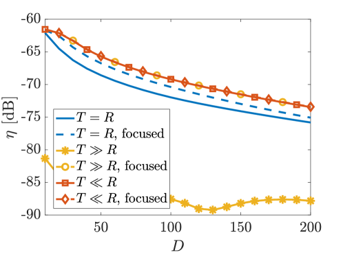
Figure 7: Path gain $\eta$ as a function of the link distance $D$ (multiples of $\lambda$).

VI-B OAM Detection

In this subsection, we characterize the OAM-based communication scheme in terms of path gain and bit error rate (BER). Fig. 7 reports the path gain $\eta$ for both the focused and unfocused cases as a function of the normalized link distance $D$. In particular, the same three configurations relative to Fig. 6(a), Fig. 6(b), and Fig. 6(c) are considered, corresponding to $T=R$, $T\gg R$ (i.e., downlink) and $T\ll R$ (i.e., uplink). Here we adopt $N=51$ to obtain the various curves since, given the information presented in Figs. 6(c), it can be inferred that this value serves as an upper bound for the number of well-coupled OAM modes. When antennas with identical radii are assumed (case $T=R=10$), the path gain is more favorable with focused OAM, which does not impact the amount of transmitted energy but allows for concentrating a larger amount of it on the receiving LIS. The gap between the unfocused and focused case is clearly visible in downlink (i.e., $T=25$, $R=5$), where the large transmitting LIS produces a great divergence of the OAM modes. If such a divergence is not properly compensated by focusing, a significant performance loss in terms of energy collected by the receiver is experienced (e.g., around $17\,$dB at $D=100$). Differently, in uplink (i.e., $T=5$, $R=25$) no difference is experienced between the focused and unfocused cases. In this configuration, (i) the small transmitting LIS is not capable of focusing the transmitted energy, (ii) the OAM beam divergence is limited by the small transmitting LIS, and (iii) the large receiving LIS is intrinsically more efficient in collecting the energy spread by the higher-order OAM modes.

Let us now concentrate on the performance of the different detection schemes that have been proposed. Fig. 8(a) depicts the BER as a function of the SNR, as defined in (31), for $R=T=10$ and $D=100$ when focused OAM and a binary phase shift keying (BPSK) modulation scheme are adopted. In particular, results are reported for a subset of OAM mode orders $\ell_{n}$, as indicated in the legend (i.e., modes with positive signs only are considered). Thanks to the MF strategy, the continuous curves coincide with the bit error probability of an optimum uncoded BPSK system, considering the fraction of energy allocated to each OAM mode. In fact, as it is possible to notice, the best performance is experienced by the OAM modes with lower indexes, which are better-coupled thanks to their limited divergence. In particular, the OAM modes for $\ell_{n}=0,1,2$ experience almost the same coupling, thus resulting in a similar performance. In the same figure, the MF performance is compared to that of the sub-optimum ID scheme. This has been implemented considering the compensation of both the quadratic phase terms at the receiving LIS and the additional phase terms with an ideal single-tap equalizer. It can be noticed that, in this case, the performance loss of the ID scheme can change drastically depending on the OAM mode order. In particular, for modes with index $\ell_{n}=2,3,4$, there is only a slight decrease in performance (below approximately $1\,$dB), while the fundamental mode for $\ell_{n}=0$ is severely impacted. This is due to the diverse waveform shapes associated with the various OAM modes and the adoption of the sub-optimum ID strategy, thus making the performance dependent on the specific signal shape, in contrast to the MF method where the performance is independent of the signal shape. In Fig. 8(b), the impact of the smart integration strategy for the ID detection, as described in Sec. V-E, is reported. In this case, an integration window corresponding to the radial coordinates where the beams exhibit a reduction of $10\,$dB from their corresponding peak was considered. The results demonstrate that the smart integration technique enhances the performance for all OAM modes, albeit to varying degrees. The amelioration is small for modes that already exhibit minimal loss compared to the MF (as observed in Fig. 8(a)). However, a substantial improvement is evident for the fundamental mode, which experiences significant performance degradation when employing the standard ID strategy. The smart integration approach facilitates the enhancement of the BER by balancing the useful and noise energies that are accumulated. Specifically, employing large integration windows results in an increased useful energy level but also a higher noise energy level. On the contrary, small integration windows limit the amount of useful signal energy but diminish the accumulated noise. Using smart integration, the performance degradation of ID with respect to the MF is highly reduced, making such a strategy a viable solution for OAM detection with significantly lower complexity. The primary limitation of the ID method is the requirement for channel estimation to compensate for the phase terms. This drawback can be circumvented by utilizing the ED strategy, whose performance assessment is reported in Fig. 8(c). In this case, the smart integration technique is applied, as for the ID approach, and the optimum detection threshold for OOK demodulation, i.e., the threshold $\zeta_{n}$ that ensures the minimum BER for each OAM mode and SNR value, is utilized. The figure displays the results for three OAM modes only to improve readability. It is evident that the performance of the ED method is inferior to that of both the MF and the ID approach due to the non-linear processing and the use of the OOK modulation. Specifically, a degradation of approximately $5\,$dB is observed. However, this approach eliminates the need for amplitude correlation or channel estimation at the receiving LIS.

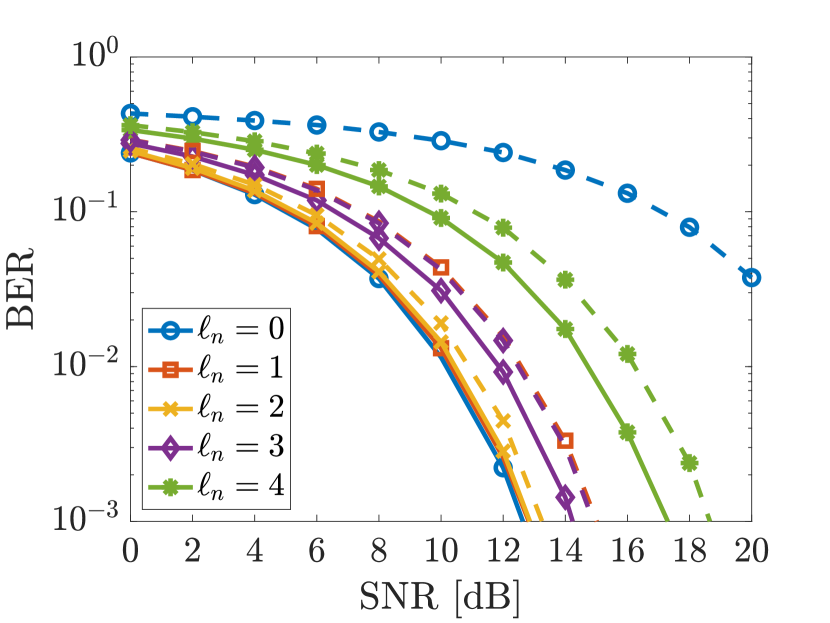
(a) MF versus ID

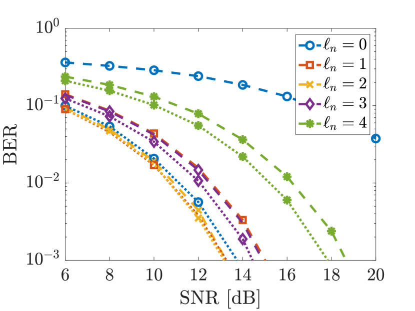
(b) ID versus ID with smart integration.

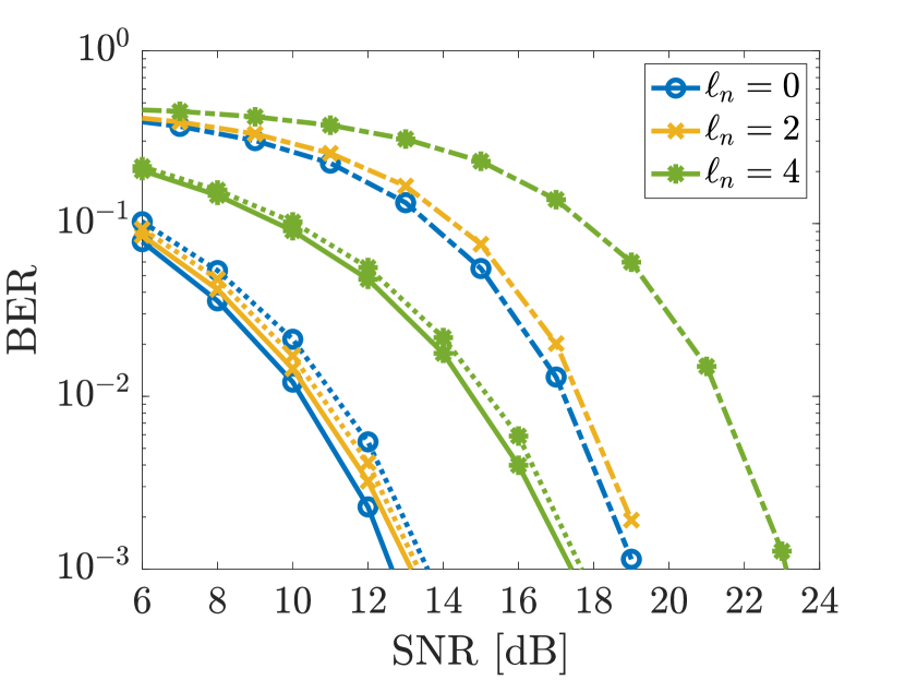
(c) MF versus ID versus ED

Figure 8: BER as a function of the SNR for different OAM modes. Continuous lines ($-$) are for the MF; dashed lines ($-\,-$) are for the ID; dotted lines ($\cdot\cdot$) are for the ID (smart integration); dot-dashed lines ($\cdot-$) are for the ED (smart integration and optimum detection threshold).

In Fig. 9, the impact of the detection threshold to discriminate between the hypotheses of noise only (i.e., $x_{n}=0$) and that of signal plus noise (i.e., $x_{n}=1$) in the OOK demodulation is reported. In the figure, the BER is reported as a function of the threshold-to-noise ratio (TNR) for different OAM mode orders $\ell_{n}$, considering a SNR of $19\,$dB, where we defined $\mathsf{TNR}=\zeta_{n}/N_{0}$, $n=1,2,\ldots,N$. It is possible to note that an optimum threshold value exists for each OAM mode. The fundamental mode (i.e., $\ell_{n}=0$), which has a higher coupling value, demonstrates the best BER. Conversely, higher-order modes exhibit degraded performance. In particular, the minimum values in Fig. 9, when considering the smart integration (dashed lines), corresponding to the BER values for an SNR of $19\,$dB in Fig. 8(c), when accounting for the ED curves. In the same figure, the ED performance as a function of the TNR, but without smart integration, is reported. As for the ID approach, the smart integration allows for improving the performance, by balancing the amount of energy and noise accumulated at the receiving LIS. Interestingly, when smart integration is not considered, the optimum threshold decreases monotonically when increasing the mode order $\ell_{n}$; in fact, the useful energy decreases accordingly due to the lower coupling, thus it is convenient to decrease the decision threshold in (41). Differently, when the smart integration approach is considered, the optimum threshold is still mode-dependent, although not exhibiting a monotonic behavior with respect to the mode order. This is reasonable since the corresponding beams are placed at different points along the radial coordinate, and the width of the integration window changes for each mode (also with a noise power $n_{n}(\rho_{\text{R}})$ which is not flat after de-multiplexing); thus, the optimum threshold must account for either the useful fraction of energy or the amount of noise energy in the specific integration window selected.

It is worth noticing that these curves assume that the same power is associated with the different OAM modes (i.e., equal power allocation at the transmitting LIS). In order to maximize the system capacity, water-filling power distribution at the transmitter side, accounting for the different coupling intensities of the OAM modes, is required.

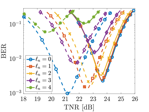
Figure 9: BER as a function of the TNR for different OAM modes and a SNR of $19\,$dB. Continuous lines ($-$) are without smart integration; dashed lines ($-\,-$) are with smart integration.

VI-C Discussion and Implementation Complexity Analysis

The exploitation of the OAM property has both practical advantages and ineluctable disadvantages. Concerning the benefits of the OAM characteristics, it has been shown that this transmission technique allows multi-modal communications, hence enabling spatial multiplexing in LOS MIMO communications. Specifically, the basis functions proposed in (17)-(18) introduce the possibility to perform spatial multiplexing with a considerably lower complexity at the transmitting LIS side with respect to the optimum SVD case. In fact, with the SVD/CPWFs approach, the basis functions depend on the overall system geometry (i.e., sizes of both circular LISs and relative distance), which needs to be known at both sides and requires a certain degree of hardware flexibility. With OAM, instead, such knowledge is not required at the transmitting LIS side (or distance only in the case of focused OAM) when operating in a paraxial regime.

On the other side, the detection of OAM-multiplexed EM fields with a receiving LIS results quite demanding in terms of complexity and knowledge of the system geometry if optimal MF processing is adopted. Differently, the complexity can be reduced, and system geometry knowledge can be relaxed if ID and ED strategies are adopted. A summary of the flexibility requirements at the transmitting (TX) and receiving (RX) LIS as well as of the required degree of knowledge at both sides is reported in Table I.

TABLE I: Implementation requirements for the different detection strategies.

	TX LIS flexibility	RX LIS flexibility	Knowledge at TX	Knowledge at RX
Optimal	Phase tapering,	Phase tapering,	RX LIS size,	TX LIS size,
SVD/CPWFs	amplitude tapering	amplitude tapering	distance	distance
TX: OAM	Phase tapering	Phase tapering,	N/A	TX LIS size,
RX: MF		amplitude tapering		distance
TX: Focused OAM	Phase tapering	Phase tapering,	Distance	TX LIS size,
RX: MF		amplitude tapering		distance
TX: OAM	Phase tapering	Phase tapering,	Distance	N/A
RX: ID		channel equalization
TX: Focused OAM	Phase tapering	Phase tapering,	Distance	N/A
RX: ID		channel equalization
TX: OAM	Phase tapering	Phase tapering,	N/A	N/A
RX: ED		non-linear processing
TX: Focused OAM	Phase tapering	Phase tapering,	Distance	N/A
RX: ED		non-linear processing

Apart from these considerations, an element of fundamental importance that is worth to be mentioned deals with the employment of large LIS antennas (i.e., holographic MIMO configuration) rather than UCAs [28]. Suppose, in fact, to exploit a large UCA to receive the OAM-multiplexed EM field, whose radius is even collimated to the radial coordinate $\rho_{\text{R}}$ corresponding to the peak of a specific mode (for example, $\ell_{n}=3$ in Fig. 2(b)). In such a case, the energy that can be collected from the other modes (e.g., that for $\ell_{n}=1$ or $\ell_{n}=6$ in Fig. 2(b)) will be inevitably low, due to the different divergence behavior spreading the beams at different radii. In this sense, the use of a large receiving LIS enables much more flexibility and larger coupling intensities for an increased number of OAM modes.

Be that as it may, OAM communications also display several, not negligible negative aspects that necessarily need to be considered. Fig. 5 highlighted that the number of the effectively well-coupled OAM modes is much smaller than that of the optimum communication modes, both in the presence and absence of focusing. Focusing has been shown to partially compensate for this OAM deficiency and is particularly important when large LISs are employed, especially at the transmitting side. Behind all that, it is essential to note that the system under consideration assumes a paraxial LOS scenario. Any misalignment between the transmitter and the receiver, such as lateral displacements or receiver angular errors, or the presence of multipath propagation, will result in power loss and potential crosstalk at the receiver side. Therefore, suitable strategies must be implemented to address these effects in more general scenarios characterized by mobility and multipath.

VII Conclusion

The paper discussed holographic MIMO communications that exploit the OAM property of EM waves, thus investigating the relationship between optimum communication modes and OAM modes. It proposed OAM-related basis functions that offer a simpler implementation than the optimum solution based on eigenfunction decomposition, although reducing the channel DoF. Various detection strategies at the receiver have been proposed and analyzed to investigate performance and complexity trade-offs. The paper also introduced focusing to improve the performance in terms of DoF and coupling strength, showing its effectiveness in different configurations. The numerical analysis demonstrated the feasibility of a significant number of orthogonal OAM channels, particularly when focusing is used to mitigate the beam divergence characteristic of OAM modes in the near field, by characterizing the performance of the proposed OAM demultiplexing and detection schemes.

Appendix A Example of OAM Amplitude and Phase Profiles

Table II displays the transmitting phase profiles and the corresponding OAM modes (both amplitude and phase patterns) obtained at the reciving LIS for different topological charges, both with and without employing focusing at the transmitting LIS when $T=R=5$ and $D=20$. In particular, results for $\ell_{n}=0$ are the beams obtained with unfocused/focused constant phase profiles along $\varphi_{\text{T}}$, thus corresponding to classical diffraction patterns of circular apertures. The increasing beam divergence, partially compensated by focusing, can be seen in the subsequent rows for increasing values of $\ell_{n}$, as well as the corresponding helical-shaped phase profiles at the receiver side.

TABLE II: Example of transmitting and receiving OAM amplitude/phase profiles, with and without focusing, for $\ell_{n}=0,1,3$ ($T=R=5$, $D=20$).

	TX phase		RX amplitude		RX phase
	Unfocused	Focused	Unfocused	Focused	Unfocused	Focused
$\ell_{n}=0$
$\ell_{n}=1$
$\ell_{n}=3$

Appendix B Noise Characterization

Let us contemplate the noise statistical characterization by expressing the noise field $n(\rho_{\text{R}},\varphi_{\text{R}})$ in Cartesian coordinates, i.e., $\tilde{n}(x,y)$. Specifically, it is

$$w_{n} =\int_{S_{\text{R}}}\tilde{n}(x,y)\tilde{F}_{n}^{*}(x,y)\,\text{d}x\text{d}y$$ (43)

where $\tilde{n}(x,y)$ is the complex AWGN with one-sided power spectral density $N_{0}$ and $\tilde{F}_{n}(x,y)$ identifies the generic $n$-th receiving template function adopted at the receiving LIS in Cartesian coordinates. We assume that this template function is in the same form of (14) when expressed in polar coordinates, i.e., $\tilde{F}_{n}(x,y)=F_{n}(\rho_{\text{R}},\varphi_{\text{R}})=f_{n}(\rho_{\text{R}})e^{\jmath\ell_{n}\varphi_{\text{R}}}$, meaning that it is separable in the radial and angular coordinates and comprises the OAM exponential term. The radial component $f_{n}(\rho_{\text{R}})$ instead is an arbitrary function that depends on the selected detection strategy. Due to the AWGN assumption in the spatial domain, the noise variance can be computed as

$$\sigma_{w}^{2} =\mathbb{E}\left[\left|w_{n}\right|^{2}\right]=\int_{S_{\text{R}}}\int_{S_{\text{R}}}\tilde{F}_{n}^{*}(x,y)\tilde{F}_{n}(x^{\prime},y^{\prime})\mathbb{E}[\tilde{n}(x,y)\tilde{n}^{*}(x^{\prime},y^{\prime})]\,\text{d}x\text{d}y\,\text{d}x^{\prime}\text{d}y^{\prime}$$

$$=N_{0}\int_{S_{\text{R}}}\left|\tilde{F}_{n}(x,y)\right|^{2}\,\text{d}x\text{d}y=N_{0}\int_{0}^{2\pi}\int_{0}^{R_{\text{R}}}\left|f_{n}(\rho_{\text{R}})e^{\jmath\ell_{n}\varphi_{\text{R}}}\right|^{2}\rho_{\text{R}}\,\text{d}\rho_{\text{R}}\text{d}\varphi_{\text{R}}$$

$$=2\pi N_{0}\int_{0}^{R_{\text{R}}}\left|f_{n}(\rho_{\text{R}})\right|^{2}\rho_{\text{R}}\,\text{d}\rho_{\text{R}}$$ (44)

where $\rho_{\text{R}}$ is the Jacobian determinant of the transformation from Cartesian to polar coordinates. Notably, the radial function $f_{n}(\rho_{\text{R}})$ adopted at the receiving LIS plays a fundamental role in determining the amount of noise power collected by the receiving LIS. In particular, for the MF case it holds $f_{n}(\rho_{\text{R}})=\psi_{n}^{\rho}(\rho_{\text{R}})$, thus leading to

$$\sigma_{w,\text{MF}}^{2} =2\pi N_{0}\int_{0}^{R_{\text{R}}}\left|\psi_{n}^{\rho}(\rho_{\text{R}})\right|^{2}\rho_{\text{R}}\,\text{d}\rho_{\text{R}}=2\pi N_{0}h_{n}^{\text{(MF)}}$$ (45)

where $h_{n}^{\text{(MF)}}=E_{n}$ is given in (37)-(38). Similarly, for the ID strategy, being $f_{n}(\rho_{\text{R}})=\Pi_{R_{\text{R}}}(\rho_{\text{R}})$, it results

$$\sigma_{w,\text{ID}}^{2} =2\pi N_{0}\int_{0}^{R_{\text{R}}}\left|\Pi_{R_{\text{R}}}(\rho_{\text{R}})\right|^{2}\rho_{\text{R}}\,\text{d}\rho_{\text{R}}=\pi N_{0}R_{\text{R}}^{2}\,.$$ (46)

While the optimal MF approach maximizes the SNR at the receiver, by perfectly equalizing the propagation effects, the noise variance of the ID scheme increases with the observation interval, i.e., the integration domain in the radial direction enlarges. For this reason, proper countermeasures such as the smart integration technique discussed in Sec. V-E should be adopted.

References

- [1] G. Torcolacci, N. Decarli, and D. Dardari, “OAM-based holographic MIMO using large intelligent surfaces,” in Proc. IEEE Global Telecomm. Conf., Dec. 2022, pp. 651–655.
- [2] G. Gradoni, M. Di Renzo, A. Diaz-Rubio, S. Tretyakov, C. Caloz, Z. Peng, A. Alu, G. Lerosey, M. Fink, V. Galdi et al., “Smart radio environments,” arXiv preprint arXiv:2111.08676, Nov. 2021.
- [3] E. Björnson, L. Sanguinetti, H. Wymeersch, J. Hoydis, and T. L. Marzetta, “Massive MIMO is a reality. What is next?: Five promising research directions for antenna arrays,” Digit. Signal Process., vol. 94, pp. 3–20, Jun. 2019.
- [4] D. Dardari and N. Decarli, “Holographic communication using intelligent surfaces,” IEEE Commun. Mag., vol. 59, no. 6, pp. 35–41, Jun. 2021.
- [5] T. Gong, I. Vinieratou, R. Ji, C. Huang, G. C. Alexandropoulos, L. Wei, Z. Zhang, M. Debbah, H. V. Poor, and C. Yuen, “Holographic MIMO communications: Theoretical foundations, enabling technologies, and future directions,” arXiv preprint arXiv:2212.01257, Dec. 2022.
- [6] L. Sanguinetti, A. A. D’Amico, and M. Debbah, “Wavenumber-division multiplexing in line-of-sight holographic MIMO communications,” IEEE Trans. Wireless Commun., pp. 1–1, Sep. 2022.
- [7] D. A. Miller, “Communicating with waves between volumes: evaluating orthogonal spatial channels and limits on coupling strengths,” Appl. Opt., vol. 39, no. 11, pp. 1681–1699, Apr. 2000.
- [8] D. Dardari, “Communicating with large intelligent surfaces: Fundamental limits and models,” IEEE J. Select. Areas Commun., vol. 38, no. 11, pp. 2526–2537, Nov. 2020.
- [9] J. Wang, J.-Y. Yang, I. Fazal, N. Ahmed, Y. Yan, H. Huang, Y. Ren, Y. Yue, S. Dolinar, M. Tur, and A. E. Willner, “Terabit free-space data transmission employing orbital angular momentum multiplexing,” Nat. Photon., vol. 6, pp. 488–496, Jun. 2012.
- [10] W. Cheng, W. Zhang, H. Jing, S. Gao, and H. Zhang, “Orbital angular momentum for wireless communications,” IEEE Wirel. Commun., vol. 26, no. 1, pp. 100–107, Dec. 2018.
- [11] L. Liang, W. Cheng, H. Zhang, Z. Li, and Y. Li, “Orbital-angular-momentum based mode-hopping: A novel anti-jamming technique,” in 2017 IEEE/CIC Int. Conf. Commun. China, Oct. 2017, pp. 1–6.
- [12] W. Cheng, H. Zhang, L. Liang, H. Jing, and Z. Li, “Orbital-angular-momentum embedded massive MIMO: Achieving multiplicative spectrum-efficiency for mmWave communications,” IEEE Access, vol. 6, pp. 2732–2745, Dec. 2017.
- [13] Z. Zhang, S. Zheng, W. Zhang, X. Jin, H. Chi, and X. Zhang, “Experimental demonstration of the capacity gain of plane spiral OAM-based MIMO system,” IEEE Microw. Wirel. Compon. Lett., vol. 27, no. 8, pp. 757–759, Jul. 2017.
- [14] Y. Yan, L. Li, G. Xie, M. Ziyadi, A. M. Ariaei, Y. Ren, O. Renaudin, Z. Zhao, Z. Wang, C. Liu, S. Sajuyigbe, S. Talwar, S. Ashrafi, A. F. Molisch, and A. E. Willner, “OFDM over mm-Wave OAM channels in a multipath environment with intersymbol interference,” in Proc. IEEE Global Telecomm. Conf., Dec. 2016, pp. 1–6.
- [15] T. Yuan, H. Wang, Y. Qin, and Y. Cheng, “Electromagnetic vortex imaging using uniform concentric circular arrays,” IEEE Antennas Wirel. Propag. Lett., vol. 15, pp. 1024–1027, Oct. 2015.
- [16] E. Mari, F. Spinello, M. Oldoni, R. A. Ravanelli, F. Romanato, and G. Parisi, “Near-field experimental verification of separation of OAM channels,” IEEE Antennas Wirel. Propag. Lett., vol. 14, pp. 556–558, Nov. 2014.
- [17] R. Chen, H. Zhou, M. Moretti, X. Wang, and J. Li, “Orbital angular momentum waves: Generation, detection, and emerging applications,” IEEE Commun. Surv. Tutor., vol. 22, no. 2, pp. 840–868, Nov. 2019.
- [18] O. Edfors and A. J. Johansson, “Is orbital angular momentum (OAM) based radio communication an unexploited area?” IEEE Trans. Antennas Propagat., vol. 60, no. 2, pp. 1126–1131, Oct. 2011.
- [19] N. Zhao, X. Li, G. Li, and J. M. Kahn, “Capacity limits of spatially multiplexed free-space communication,” Nat. Photon., vol. 9, no. 12, pp. 822–826, Nov. 2015.
- [20] M. Tamagnone, C. Craeye, and J. Perruisseau-Carrier, “Comment on ‘Encoding many channels on the same frequency through radio vorticity: first experimental test’,” New J. Phys., vol. 14, no. 11, p. 118001, Nov. 2012.
- [21] M. Oldoni, F. Spinello, E. Mari, G. Parisi, C. G. Someda, F. Tamburini, F. Romanato, R. A. Ravanelli, P. Coassini, and B. Thidé, “Space-division demultiplexing in orbital-angular-momentum-based MIMO radio systems,” IEEE Trans. Antennas Propagat., vol. 63, no. 10, pp. 4582–4587, Jul. 2015.
- [22] R. Gaffoglio, A. Cagliero, G. Vecchi, and F. P. Andriulli, “Vortex waves and channel capacity: Hopes and reality,” IEEE Access, vol. 6, pp. 19 814–19 822, Dec. 2017.
- [23] L. Allen, M. W. Beijersbergen, R. J. C. Spreeuw, and J. P. Woerdman, “Orbital angular momentum of light and the transformation of Laguerre-Gaussian laser modes,” Phys. Rev. A, vol. 45, pp. 8185–8189, Jun. 1992.
- [24] M. Beijersbergen, L. Allen, H. van der Veen, and J. Woerdman, “Astigmatic laser mode converters and transfer of orbital angular momentum,” Opt. Commun., vol. 96, no. 1-3, Aug. 1992.
- [25] B. Thidé, H. Then, J. Sjöholm, K. Palmer, J. Bergman, T. Carozzi, Y. N. Istomin, N. Ibragimov, and R. Khamitova, “Utilization of photon orbital angular momentum in the low-frequency radio domain,” Phys. Rev. Lett., vol. 99, no. 8, p. 087701, Aug. 2007.
- [26] S. M. Mohammadi, L. K. S. Daldorff, J. E. S. Bergman, R. L. Karlsson, B. Thide, K. Forozesh, T. D. Carozzi, and B. Isham, “Orbital angular momentum in radio—A system study,” IEEE Trans. Antennas Propagat., vol. 58, no. 2, pp. 565–572, Dec. 2009.
- [27] L. Allen, M. Padgett, and M. Babiker, “IV. The Orbital Angular Momentum of Light,” ser. Progress in Optics, E. Wolf, Ed. Elsevier, 1999, vol. 39, pp. 291–372.
- [28] R. Chen, W.-X. Long, X. Wang, and L. Jiandong, “Multi-mode OAM radio waves: Generation, angle of arrival estimation and reception with UCAs,” IEEE Trans. Wireless Commun., vol. 19, no. 10, pp. 6932–6947, Jul. 2020.
- [29] A. Cagliero and R. Gaffoglio, “On the spectral efficiency limits of an OAM-based multiplexing scheme,” IEEE Antennas Wirel., vol. 16, pp. 900–903, Oct. 2017.
- [30] E. Cano and B. Allen, “Multiple-antenna phase-gradient detection for OAM radio communications,” Electron. Lett., vol. 51, no. 9, pp. 724–725, Apr. 2015.
- [31] Y. Hu, S. Zheng, Z. Zhang, H. Chi, X. Jin, and X. Zhang, “Simulation of orbital angular momentum radio communication systems based on partial aperture sampling receiving scheme,” IET Microw. Antennas Propag., vol. 10, no. 10, pp. 1043–1047, Jul. 2016.
- [32] A. Affan, S. Mumtaz, H. M. Asif, and L. Musavian, “Performance analysis of orbital angular momentum (OAM): A 6G waveform design,” IEEE Commun. Lett., vol. 25, no. 12, pp. 3985–3989, Sep. 2021.
- [33] W. Zhang, S. Zheng, X. Hui, R. Dong, X. Jin, H. Chi, and X. Zhang, “Mode division multiplexing communication using microwave orbital angular momentum: An experimental study,” IEEE Trans. Wireless Commun., vol. 16, no. 2, pp. 1308–1318, Feb. 2017.
- [34] Y. Ren, L. Li, G. Xie, Y. Yan, Y. Cao, H. Huang, N. Ahmed, Z. Zhao, P. Liao, C. Zhang, G. Caire, A. F. Molisch, M. Tur, and A. E. Willner, “Line-of-sight millimeter-wave communications using orbital angular momentum multiplexing combined with conventional spatial multiplexing,” IEEE Trans. Wireless Commun., vol. 16, no. 5, pp. 3151–3161, Mar. 2017.
- [35] Z. Yang, Y. Hu, Z. Zhang, W. Xu, C. Zhong, and K.-K. Wong, “Reconfigurable intelligent surface based orbital angular momentum: Architecture, opportunities, and challenges,” IEEE Wirel. Commun., vol. 28, no. 6, pp. 132–137, 2021.
- [36] H. Xue, J. Han, S. Zhang, Y. Tian, J. Hou, and L. Li, “Co-modulation of spin angular momentum and high-order orbital angular momentum based on anisotropic holographic metasurfaces,” IEEE Trans. Antennas Propagat., pp. 1–1, Feb. 2023.
- [37] H. Yang, S. Zheng, H. Zhang, N. Li, D. Shen, T. He, Z. Yang, Z. Lyu, and X. Yu, “A THz-OAM wireless communication system based on transmissive metasurface,” IEEE Trans. Antennas Propagat., pp. 1–1, Mar. 2023.
- [38] R. Chen, M. Chen, X. Xiao, W. Zhang, and J. Li, “Multi-user orbital angular momentum based terahertz communications,” IEEE Trans. Wireless Commun., pp. 1–1, Feb. 2023.
- [39] X. Su, H. Song, H. Zhou, K. Zou, Y. Duan, N. Karapetyan, R. Zhang, A. Minoofar, H. Song, K. Pang, S. Zach, A. F. Molisch, M. Tur, and A. E. Willner, “A THz integrated circuit based on a pixel array to mode multiplex two 10-Gbit/s QPSK channels each on a different OAM beam,” J. Light. Technol., vol. 41, no. 4, pp. 1095–1103, Sep. 2023.
- [40] Z. Zhao, R. Zhang, H. Song, K. Pang, A. Almaiman, H. Zhou, H. Song, C. Liu, N. Hu, X. Su et al., “Modal coupling and crosstalk due to turbulence and divergence on free space THz links using multiple orbital angular momentum beams,” Sci. Rep., vol. 11, no. 1, p. 2110, Jan. 2021.
- [41] A. E. Willner, X. Su, H. Zhou, A. Minoofar, Z. Zhao, R. Zhang, M. Tur, A. F. Molisch, D. Lee, and A. Almaiman, “High capacity terahertz communication systems based on multiple orbital-angular-momentum beams,” J. Opt., vol. 24, no. 12, p. 124002, Nov. 2022.
- [42] S. Tretyakov, “Metasurfaces for general transformations of electromagnetic fields,” Philos. Trans., vol. 373, Aug. 2015.
- [43] A. Silva, F. Monticone, G. Castaldi, V. Galdi, A. Alù, and N. Engheta, “Performing mathematical operations with metamaterials,” Science, vol. 343, no. 6167, pp. 160–163, Jan. 2014.
- [44] D. González-Ovejero, G. Minatti, G. Chattopadhyay, and S. Maci, “Multibeam by metasurface antennas,” IEEE Trans. Antennas Propagat., vol. 65, no. 6, pp. 2923–2930, Feb. 2017.
- [45] N. Decarli and D. Dardari, “Communication modes with large intelligent surfaces in the near field,” IEEE Access, vol. 9, pp. 165 648–165 666, Dec. 2021.
- [46] J. Xu, “Degrees of freedom of OAM-based line-of-sight radio systems,” IEEE Trans. Antennas Propagat., vol. 65, no. 4, pp. 1996–2008, Apr. 2017.
- [47] B. Thidé and F. Tamburini, “The physics of angular momentum radio,” in 2015 1st URSI AT-RASC. IEEE, May 2015, pp. 1–1.
- [48] L. Allen, M. W. Beijersbergen, R. J. C. Spreeuw, and J. P. Woerdman, “Orbital angular momentum of light and the transformation of laguerre-gaussian laser modes,” Phys. Rev. A, vol. 45, pp. 8185–8189, Jun. 1992.
- [49] S. M. Barnett, L. Allen, R. P. Cameron, C. R. Gilson, M. J. Padgett, F. C. Speirits, and A. M. Yao, “On the natures of the spin and orbital parts of optical angular momentum,” J. Opt., vol. 18, no. 6, p. 064004, Apr. 2016.
- [50] C. Liu, J. Liu, L. Niu, X. Wei, K. Wang, and Z. Yang, “Terahertz circular Airy vortex beams,” Sci. Rep., vol. 7, no. 1, pp. 1–8, Jun. 2017.
- [51] R. Kadlimatti and P. V. Parimi, “Millimeter-wave nondiffracting circular Airy OAM beams,” IEEE Trans. Antennas Propagat., vol. 67, no. 1, pp. 260–269, Oct. 2018.
- [52] D. A. Miller, “Waves, modes, communications, and optics: a tutorial,” Adv. Opt. Photonics., vol. 11, no. 3, pp. 679–825, Sep. 2019.
- [53] S. M. Mohammadi, L. K. S. Daldorff, J. E. S. Bergman, R. L. Karlsson, B. Thide, K. Forozesh, T. D. Carozzi, and B. Isham, “Orbital angular momentum in radio—a system study,” IEEE Trans. Antennas Propagat., vol. 58, no. 2, pp. 565–572, Feb. 2010.
- [54] C. Balanis, Antenna Theory: Analysis and Design. Wiley, 2015.
- [55] G. Xie, L. Li, Y. Ren, H. Huang, Y. Yan, N. Ahmed, Z. Zhao, M. P. J. Lavery, N. Ashrafi, S. Ashrafi, R. Bock, M. Tur, A. F. Molisch, and A. E. Willner, “Performance metrics and design considerations for a free-space optical orbital-angular-momentum-multiplexed communication link,” Optica, vol. 2, no. 4, pp. 357–365, Apr. 2015.
- [56] P. Nepa and A. Buffi, “Near-field-focused microwave antennas: Near-field shaping and implementation.” IEEE Antennas Propagat. Mag., vol. 59, no. 3, pp. 42–53, ApR. 2017.
- [57] E. Björnson, Ö. T. Demir, and L. Sanguinetti, “A primer on near-field beamforming for arrays and reconfigurable intelligent surfaces,” in Proc. 55th Asilomar Conf. on Signals, Systems and Computers. IEEE, Nov. 2021, pp. 105–112.
- [58] A. de Jesus Torres, L. Sanguinetti, and E. Björnson, “Electromagnetic interference in RIS-aided communications,” IEEE Wireless Commun. Lett., vol. 11, no. 4, pp. 668–672, Nov. 2022.
- [59] N. Decarli, A. Giorgetti, D. Dardari, M. Chiani, and M. Z. Win, “Stop-and-go receivers for non-coherent impulse communications,” IEEE Trans. Wireless Commun., vol. 13, no. 9, pp. 4821–4835, Jul. 2014.
- [60] N. Decarli, A. Giorgetti, D. Dardari, and M. Chiani, “Blind integration time determination for UWB transmitted reference receivers,” in Proc. IEEE Global Telecomm. Conf. IEEE, Dec. 2011, pp. 1–5.
- [61] M. A. Nemati, U. Mitra, and R. A. Scholtz, “Optimum integration time for UWB transmitted reference and energy detector receivers,” in MILCOM 2006-2006 IEEE Mil. Commun. Conf. IEEE, Oct. 2006, pp. 1–7.