Super-exponential convergence rate of a nonlinear continuous data assimilation algorithm: The 2D Navier-Stokes equations paradigm

Abstract.

We study a nonlinear-nudging modification of the Azouani-Olson-Titi continuous data assimilation (downscaling) algorithm for the 2D incompressible Navier-Stokes equations. We give a rigorous proof that the nonlinear-nudging system is globally well-posed, and moreover that its solutions converge to the true solution exponentially fast in time. Furthermore, we also prove that, once the error has decreased below a certain order one threshold, the convergence becomes double-exponentially fast in time, up until a precision determined by the sparsity of the observed data. In addition, we demonstrate the applicability of the analytical and sharpness of the results computationally.

1. Introduction

Many dissipative dynamical systems that model physical processes are chaotic and highly sensitive to initial conditions. Hence, having incomplete information about initial conditions makes simulating these systems accurately a difficult task. To overcome this issue in practice, the available spatially discrete observed data can be used to inform the model via a wide variety of techniques, collectively known as data assimilation. Data assimilation can be done using a variety of different methods incorporate observations into the mathematical model generally using either statistical or continuous techniques. In this paper, we focus on a continuous data assimilation (CDA) algorithm, also known as the Azouani-Olson-Titi (AOT) algorithm. The CDA algorithm is based on the mathematical theory that many dissipative evolution equations describing fluid flow have solutions that are, in large-time, determined uniquely by the values of their solutions at a finite number of adequately distributed nodes or modes (see, e.g. [44] and references therein). It incorporates observational data into the model at the partial differential equation (PDE) level using a feedback control (nudging) term. This paper investigates the convergence of a nonlinear-nudging version of the CDA algorithm.

The CDA algorithm was first introduced in [4, 5] (see also [16, 54, 70, 71] for early ideas in this direction). The algorithm considers a dissipative dynamical system

(1.1) $$\frac{d\mathbf{u}}{dt}=\mathcal{F}(\mathbf{u}),$$

with an unknown initial condition. We denote a given interpolation of the observations of the unknown reference solution $\mathbf{u}$ at course spatial scales by $I_{h}(\mathbf{u})$, where $h$ is some characteristic length scale of the the observational data (e.g., the average spatial distance between observations). These observations are incorporated via a feedback control term in the following modified system

(1.2a) $$\frac{d\mathbf{v}}{dt} =\mathcal{F}(\mathbf{v})+\mu(I_{h}(\mathbf{u})-I_{h}(\mathbf{v})),$$

(1.2b) $$\hskip 28.90755pt\mathbf{v}(t=0)=\mathbf{v}_{0},$$

where $\mu>0$ is an adequately chosen positive relaxation (nudging) parameter and $\mathbf{v}_{0}$ is any sufficiently smooth initial condition. A wide class of standard interpolants $I_{h}$ are admissible by the analysis of [4] including, e.g., piecewise constant interpolation, linear interpolation, and Fourier truncation, among others, making this algorithm very adaptable for physical models and computationally inexpensive to implement. In the context of the 2D incompressible Navier-Stokes equations with both no-slip and periodic boundary conditions, the global well-posedness of (1.2) and exponential convergence in time to the reference solution $\mathbf{u}$ of (1.1) were proven in [4]. This algorithm was then investigated in the context of numerous dissipative dynamical systems under a variety of assumptions including noisy data, incorrect parameters, incorrect models, data provided discretely in time, and assimilation of only some instead of all state variables, in, e.g., [1, 2, 3, 6, 8, 9, 10, 11, 12, 13, 14, 18, 19, 20, 21, 22, 23, 17, 24, 32, 25, 30, 31, 33, 36, 37, 38, 39, 40, 41, 42, 43, 47, 45, 46, 48, 49, 50, 52, 53, 55, 56, 57, 58, 61, 62, 63, 64, 65, 66, 67, 68, 69, 72, 73, 74, 76, 79, 81, 82, 83, 84] and the references therein.). In each of these papers exponential convergence either to $0$ or up to a certain measurable error regardless of the choice of initial conditions, and the slight modification required to existing models makes the CDA algorithm an efficient and effective data assimilation algorithm. Classical data assimilation methods are generally statistical in nature, including the Kalman filter and its variants as well as 4DVAR, but these methods are non-trivial to implement and computationally much more expensive than simply running a simulation of the dynamical system alone, making the CDA algorithm a more efficient and potentially viable alternative for use in certain real world models (see, e.g., [30, 31, 21]).

The motivation for this work comes from the computational study [61], which introduced and investigated a nonlinear version of the CDA algorithm in the context of the Kuramoto-Sivashinsky equations. This nonlinear-nudging algorithm computationally demonstrated super-exponential convergence in time to the reference solution for the 1D Kuramoto-Sivashinsky equations. This was later demonstrated with a similar modification in a computational study on the 2D magnetohydrodynamic equations in [55]. In [33], the authors adapted the nonlinear-nudging data assimilation schemes of [61] to the context of the Lorenz equation, and proved exponential (but not super-exponential) convergence. Note that another nonlinear approach to nudging was proposed and studied in [51], but using a very different method from that in the present work. In our case, in order to simplify the practical implementation, we consider the following nonlinear-nudging system of equations:

(1.3a) $$\mathbf{v}_{t} =\mathcal{F}(\mathbf{v})+\mu\mathcal{N}(I_{h}(\mathbf{u})-I_{h}(\mathbf{v}))+\beta(I_{h}(\mathbf{u})-I_{h}(\mathbf{v})),$$

(1.3b) $$\mathbf{v}(\mathbf{x},0) =\mathbf{v}_{0}(\mathbf{x}),$$

where we denote, with $\gamma\in[0,1)$,

$$\mathcal{N}(\boldsymbol{\phi}):=\begin{cases}0,&\text{ if }\quad\|\boldsymbol{\phi}\|_{L^{2}(\Omega)}=0,\\ \boldsymbol{\phi}\|\boldsymbol{\phi}\|_{L^{2}(\Omega)}^{-\gamma},&\text{ if }\quad\|\boldsymbol{\phi}\|_{L^{2}(\Omega)}>0.\end{cases}$$

Note that we formally recover the linear-nudging CDA algorithm when $\gamma=0$. As demonstrated computationally in [55, 61], we expect that once $\|I_{h}(\mathbf{u})-I_{h}(\mathbf{v})\|_{L^{2}(\Omega)}<1$, the error of the nonlinear-nudging algorithm should enjoy a super-exponential decay rate and reach machine precision at an earlier time than the linear-nudging algorithm.

We anticipate that this formulation should yield double exponential convergence of the algorithm if $\gamma\in(0,1)$. The paradigm equations used to demonstrate the convergence of this combined linear/nonlinear-nudging algorithm are the 2D incompressible Navier-Stokes equations. Indeed we prove here, with certain reasonable assumptions on $I_{h}$ and given a sufficiently developed reference flow, a double-exponential decay rate of the error, at least down to a level $\epsilon>0$, determined by $h$ and the $L^{2}$ norm (the size) of the initial data of the reference solution $\mathbf{u}$ (but otherwise independent of the initial data), and other physical parameters in the system (see Theorem 4.1 below for details). We also prove that after the precision $\epsilon$ is reached, which happens in finite time, the error continues to decay to zero at least at an exponential rate.

We believe the $\epsilon$ barrier for super-exponential convergence discussed above is likely insurmountable due to 1) a direct observation from the method of proof (see Remark 4.2), and 2) a heuristic argument of the same observation for a more general dissipative system in Appendix 7.1. Namely, as can be seen by the arguments Appendix 7.1, the nonlinear term $\mathcal{N}(I_{h}(\mathbf{u})-I_{h}(\mathbf{v}))$ in (1.3a) forces the large spatial scales (e.g., low modes) to converge at a super-exponential rate; however, this process seems to eventually destabilize the smaller spatial scales so much that they cannot be suppressed and stabilized by the linear viscous effect, obstructing super-exponential convergence after error becomes sufficiently small. Therefore, we expect to see super-exponential convergence rates for early times, which then become merely exponential for later times once the error becomes very small. Indeed, this is what we observe in the simulations in Section 5.

The paper is organized as follows: in Section 2 we lay out notation and state definitions and preliminary theorems and results for reference; in Section 3 we prove a global well-posedness result for the nonlinear-nudging system (2.3); in Section 4 we prove the convergence results discussed above; in Section 5 we investigate our results in simulations. Concluding remarks are in Section 6.

2. Preliminaries

The convergence of the nonlinear-nudging CDA algorithm will be proved in this paper in the context of the 2D incompressible Navier-Stokes equations, as a paradigm, with periodic boundary conditions. However, the result is equally valid for general dissipative systems of equations with physical boundary conditions. We begin by stating some preliminary theoretical foundations. First, the initial-boundary value problem

(2.1a) $$\mathbf{u}_{t}+\mathbf{u}\cdot\nabla\mathbf{u}-\nu\triangle\mathbf{u}+\nabla p =\mathbf{f}, \text{in }\Omega\times(0,T),$$

(2.1b) $$\nabla\cdot\mathbf{u} =0, \text{in }\Omega\times(0,T),$$

(2.1c) $$\mathbf{u}(\cdot,0) =\mathbf{u}_{0}(\cdot), \text{in }\Omega,$$

determines the reference solution for the data assimilation system, where $\mathbf{u}$ is the velocity, $p$ is the pressure, $\nu>0$ is viscosity, $\Omega=\mathbb{T}^{2}=\mathbb{R}^{2}/\mathbb{Z}^{2}$ is the domain (and hence the domain has unit length $L=1$), $T>0$, $\mathbf{f}$ is some forcing, $\mathbf{u}_{0}$ is the initial condition, and the system is equipped with periodic boundary conditions.

The linear-nudging CDA algorithm applied to the 2D incompressible Navier-Stokes equations (2.1) yields the system, with $\mu>0$ a constant,

(2.2a) $$\mathbf{v}_{t}+\mathbf{v}\cdot\nabla\mathbf{v}-\nu\triangle\mathbf{v}+\nabla\widetilde{q} =\mathbf{f}+\mu(I_{h}(\mathbf{u})-I_{h}(\mathbf{v})), \text{in }\Omega\times(0,T),$$

(2.2b) $$\nabla\cdot\mathbf{v} =0, \text{in }\Omega\times(0,T),$$

(2.2c) $$\mathbf{v}(\cdot,0) =\mathbf{v}_{0}(\cdot), \text{in }\Omega.$$

The nonlinear-nudging CDA algorithm applied to the 2D incompressible Navier-Stokes equations (2.1) yields the system, with constants $\mu,\beta>0$,

(2.3a) $$\mathbf{v}_{t}+\mathbf{v}\cdot\nabla\mathbf{v}-\nu\triangle\mathbf{v}+\nabla q =\mathbf{f}+\mu\mathcal{N}(I_{h}(\mathbf{u})-I_{h}(\mathbf{v}))$$

$$\qquad+\beta(I_{h}(\mathbf{u})-I_{h}(\mathbf{v})), \text{in }\Omega\times(0,T),$$

(2.3b) $$\nabla\cdot\mathbf{v} =0, \text{in }\Omega\times(0,T),$$

(2.3c) $$\mathbf{v}(\cdot,0) =\mathbf{v}_{0}(\cdot), \text{in }\Omega.$$

We recall the following well-known spaces. Let

$$\mathcal{V}=\{\mathbf{u}\in\dot{C}_{\text{p}}^{\infty}(\Omega):\nabla\cdot\mathbf{u}=0\},$$

where $\dot{C}_{\text{p}}^{\infty}(\Omega)$ is the space of infinitely differentiable, mean-free, periodic functions on the torus. We denote $H$ to be the closure of $\mathcal{V}$ in $L^{2}$ and $V$ to be the closure of $\mathcal{V}$ in $H^{1}$. The inner-product on $H$ is the usual $L^{2}$ inner-product,

$$(\mathbf{u},\mathbf{v}):=\int_{\Omega}\sum\limits_{i,j=1}^{2}u_{i}(\mathbf{x})v_{j}(\mathbf{x})d\mathbf{x},\quad\mathbf{u},\mathbf{v}\in H,$$

and we denote the inner-product on $V$ by

$$((\mathbf{u},\mathbf{v})):=\int_{\Omega}\sum\limits_{i,j=1}^{2}\frac{\partial u_{j}}{\partial x_{i}}(\mathbf{x})\frac{\partial v_{j}}{\partial x_{i}}(\mathbf{x})d\mathbf{x},\quad\mathbf{u},\mathbf{v}\in V.$$

These yield the following norms.

$$\|\mathbf{u}\|_{H}:=\sqrt{(\mathbf{u},\mathbf{u})},\qquad\|\mathbf{u}\|_{V}:=\sqrt{((\mathbf{u},\mathbf{u}))}.$$

Note that the definiteness of the V-norm follows from the Poincaré inequality (see, e.g., [27], [35], [78]).

We denote the Leray projector as $P_{\sigma}:\dot{L}^{2}(\Omega)\to H$, where for smooth functions $\mathbf{w}$, $P_{\sigma}\mathbf{w}=\mathbf{w}-\nabla\triangle^{-1}\nabla\cdot\mathbf{w}$, (the inverse Laplacian being computed with respect to periodic boundary conditions and the mean-free condition), and $P_{\sigma}$ is extended to $\dot{L}^{2}(\Omega)$ by continuity (see, e.g., [27, 78]). We denote $A:\mathcal{D}(A)\to H$ and $B:V\times V\to V^{*}$, where $A$ and $B$ are continuous extensions of the operators

$$A\mathbf{u} =-P_{\sigma}\triangle\mathbf{u},\qquad\qquad\mathbf{u}\in\mathcal{V},$$

$$B(\mathbf{u},\mathbf{v}) =P_{\sigma}((\mathbf{u}\cdot\nabla)\mathbf{v}),\qquad\mathbf{u},\mathbf{v}\in\mathcal{V},$$

where $\mathcal{D}(A):=V\cap H^{2}(\Omega)$. Note that $A$ is a linear, self-adjoint, and positive definite operator with compact inverse, so there exists an orthonormal basis of eigenfunctions $\left\{\mathbf{w}_{i}\right\}_{i\in\mathbb{N}}$ in $H$ such that $A\mathbf{w}_{i}=\lambda_{i}\mathbf{w}_{i}$, with eigenvalues $\lambda_{i}>0$ that are monotonically nondecreasing in $i$ (see, e.g., [27, 78, 75]). Moreover, observe in this case (the case of periodic boundary conditions) that $A=-\triangle$. Furthermore, the following versions of Poincaré inequality hold,

$$\lambda_{1}\|\mathbf{u}\|_{H}^{2}\leq\|\nabla\mathbf{u}\|_{H}^{2}\;\text{ for }\mathbf{u}\in V,$$

$$\lambda_{1}\|\nabla\mathbf{u}\|_{H}^{2}\leq\|A\mathbf{u}\|_{H}^{2}\;\text{ for }\mathbf{u}\in\mathcal{D}(A),$$

where $\lambda_{1}=4\pi^{2}$ is the first eigenvalue of the Stokes operator on $\Omega$.

Moreover, the bilinear operator, $B$, has the property that

(2.4) $$\left<B(\mathbf{u},\mathbf{v}),\mathbf{w}\right>_{V^{*},V}=-\left<B(\mathbf{u},\mathbf{w}),\mathbf{v}\right>_{V^{*},V}$$

for all $\mathbf{u},\mathbf{v},\mathbf{w}\in V$; below, we denote $\left<\cdot,\cdot\right>:=\left<\cdot,\cdot\right>_{V^{*},V}$. This implies the following identity

(2.5) $$\left<B(\mathbf{u},\mathbf{v}),\mathbf{v}\right>=0$$

for all $\mathbf{u},\mathbf{v}\in V$. Finally, the following standard inequalities hold (see, e.g., [27, 44, 75, 78, 77])

(2.6) $$|\left<B(\mathbf{u},\mathbf{v}),\mathbf{w}\right>| \leq c\|\mathbf{u}\|_{H}^{1/2}\|\mathbf{u}\|_{V}^{1/2}\|\mathbf{v}\|_{V}\|\mathbf{w}\|_{H}^{1/2}\|\mathbf{w}\|_{V}^{1/2},\text{ for }\mathbf{u},\mathbf{v},\mathbf{w}\in V,$$

(2.7) $$|\left<B(\mathbf{u},\mathbf{v}),\mathbf{w}\right>| \leq c\|\mathbf{u}\|_{H}^{1/2}\|A\mathbf{u}\|_{H}^{1/2}\|\mathbf{v}\|_{V}\|\mathbf{w}\|_{H},\text{ for }\mathbf{u}\in\mathcal{D}(A),\mathbf{v}\in V,\mathbf{w}\in H.$$

In this setting of 2D periodic boundary conditions, the following identity holds (see, e.g., [27, 75, 78])

(2.8) $$(B(\mathbf{w},\mathbf{w}),A\mathbf{w})=0\text{ for every }\mathbf{w}\in\mathcal{D}(A).$$

This implies the identity

(2.9) $$(B(\mathbf{u},\mathbf{w}),A\mathbf{w})+(B(\mathbf{w},\mathbf{u}),A\mathbf{w})=-(B(\mathbf{w},\mathbf{w}),A\mathbf{u})\text{ for all }\mathbf{u},\mathbf{w}\in\mathcal{D}(A).$$

We assume that $\mathbf{f}\in L^{\infty}(0,T;H)$ so that $P_{\sigma}\mathbf{f}=\mathbf{f}$ (without loss of generality, since the gradient part of $\mathbf{f}$ can be absorbed into the pressure gradient). Formally applying the Leray projection to (2.1) yields the equivalent evolution system

(2.10) $$\mathbf{u}_{t}+B(\mathbf{u},\mathbf{u})+\nu A\mathbf{u}=\mathbf{f},$$

(2.11) $$\mathbf{u}(\mathbf{x},0)=\mathbf{u}_{0}(\mathbf{x}).$$

Similarly, the Leray projection can be formally applied to (2.2) to obtain the system

(2.12) $$\mathbf{v}_{t}+B(\mathbf{v},\mathbf{v})+\nu A\mathbf{v} =\mathbf{f}+\mu P_{\sigma}(I_{h}(\mathbf{u})-I_{h}(\mathbf{v})),$$

(2.13) $$\mathbf{v}(\mathbf{x},0) =\mathbf{v}_{0}(\mathbf{x}).$$

and to (2.3) to obtain the system

(2.14) $$\mathbf{v}_{t}+B(\mathbf{v},\mathbf{v})+\nu A\mathbf{v} =\mathbf{f}+\mu P_{\sigma}\mathcal{N}(I_{h}(\mathbf{u})-I_{h}(\mathbf{v})),$$

$$\qquad+\beta P_{\sigma}(I_{h}(\mathbf{u})-I_{h}(\mathbf{v})),$$

(2.15) $$\mathbf{v}(\mathbf{x},0) =\mathbf{v}_{0}(\mathbf{x}).$$

where for all $\mathbf{w}\in L^{2}(\Omega)$, we recall $\mathcal{N}(\mathbf{w}):=\begin{cases}\|\mathbf{w}\|_{H}^{-\gamma}\mathbf{w},&\|\mathbf{w}\|_{H}\neq 0,\\ 0,&\|\mathbf{w}\|_{H}=0.\end{cases}$

Note that, with this choice of $\mathcal{N}$, $\mu$ has units $(\text{length})^{2\gamma}/(\text{time})^{1+\gamma}$, whereas $\beta$ has units $1/(\text{time})$.

The pressure gradient can be recovered by employing the following corollary of de Rham’s Theorem (see, e.g., [78, 44, 80]):

$$\mathbf{g}=\nabla p\text{ with }p\text{ a distribution if and only if }\left<\mathbf{g},\mathbf{h}\right>=0\text{ for all }\mathbf{h}\in\mathcal{V}.$$

Under this framework, we define the notion of a strong solution for the systems (2.10), (2.12), and (2.14) (see, e.g., [27, 75, 78, 44]).

Definition 2.1.

A strong solution of (2.10), (2.12), or (2.14) is a function $\mathbf{u}\in C([0,T];V)\cap L^{2}(0,T;\mathcal{D}(A))$ such that the equality in the system (2.10), (2.12), or (2.14) is satisfied in $L^{2}(0,T;H)$, and its time derivative $\frac{d\mathbf{u}}{dt}\in L^{2}(0,T;H)$.

We cite the classical result of the existence of global strong solutions for (2.1)

Theorem 2.2.

Given initial data $\mathbf{u}_{0}\in V$ and a forcing function $\mathbf{f}\in L^{2}(0,T;H)$, there exists a unique strong solution to (2.10) $\mathbf{u}$ such that $\mathbf{u}\in C([0,T];V)\cap L^{2}(0,T;\mathcal{D}(A))$ and $\frac{d\mathbf{u}}{dt}\in L^{2}(0,T;H)$.

For (2.10), we denote the dimensionless Grashof number as

(2.16) $$G =\frac{1}{\lambda_{1}\nu^{2}}\limsup\limits_{t\to\infty}\|\mathbf{f}(t)\|_{H}.$$

The following theorem, see, e.g., [75, 78, 27, 44, 29], details results on the large-time behavior of the strong solutions to (2.1).

Theorem 2.3.

Fix $T>0$. Suppose that $\mathbf{u}$ is a strong solution of $\eqref{NSEtrue}$, corresponding to the initial data $\mathbf{u}_{0}\in V$. Then there exists a time $t_{0}\geq 0$ which depends on $\|\mathbf{u}_{0}\|_{H}$ such that for all $t\geq t_{0}$,

(2.17) $$\|\mathbf{u}(t)\|_{H}^{2}\leq 2G^{2}\nu^{2}\;\text{ and }\int\limits_{t}^{t+T}\|\mathbf{u}(\tau)\|_{V}^{2}d\tau\leq 2\left(1+T\lambda_{1}\nu\right)G^{2}\nu,$$

moreover

(2.18) $$\|\mathbf{u}(t)\|_{V}^{2}\leq 2\lambda_{1}G^{2}\nu^{2},\qquad\int\limits_{t}^{t+T}\|A\mathbf{u}(\tau)\|_{H}^{2}d\tau\leq 2\left(1+T\lambda_{1}\nu\right)\lambda_{1}G^{2}\nu.$$

Furthermore, if $\mathbf{f}\in H$ is time-independent then

(2.19) $$\|A\mathbf{u}(t)\|_{H}^{2}\leq\lambda_{1}^{2}\nu^{2}c(1+G)^{4}.$$

We assume throughout the present work that the operator $I_{h}$ is a linear operator satisfying the following conditions

(2.20a) $$\|\boldsymbol{\phi}-I_{h}(\boldsymbol{\phi})\|_{L^{2}(\Omega)}^{2} \leq c_{0}h^{2}\|\nabla\boldsymbol{\phi}\|_{L^{2}(\Omega)}^{2},\text{ for all }\boldsymbol{\phi}\in\dot{H}^{1}(\Omega),$$

(2.20b) $$\int_{\Omega}I_{h}(\boldsymbol{\phi}) =0\text{ whenever }\int_{\Omega}\boldsymbol{\phi}=0.$$

In our theorems, we make various additional assumptions about the interpolant $I_{h}$. We record these here for reference, though we note that some of our theorems hypothesize only a subset of these assumptions.

(2.21a) $$I_{h}^{2} =I_{h},$$

(2.21b) $$(I_{h}(\boldsymbol{\phi}),\boldsymbol{\psi}) =(\boldsymbol{\phi},I_{h}(\boldsymbol{\psi}))\text{ for all }\boldsymbol{\phi},\boldsymbol{\psi}\in\dot{L}^{2}(\Omega),$$

(2.21c) $$(I_{h}\boldsymbol{\phi},\boldsymbol{\phi}) \geq 0\text{ for all }\boldsymbol{\phi}\in\dot{L}^{2}(\Omega),$$

(2.21d) $$\|I_{h}\boldsymbol{\phi}\|_{L^{2}(\Omega)} \leq\alpha\|\boldsymbol{\phi}\|_{L^{2}(\Omega)}\text{ for some }\alpha>0\text{ and for all }\boldsymbol{\phi}\in\dot{L}^{2}(\Omega),$$

(2.21e) $$(I_{h}\boldsymbol{\phi},A\boldsymbol{\phi}) \geq 0\text{ and for all }\boldsymbol{\phi}\in\mathcal{D}(A).$$

Note that Fourier truncation and local averaging over finite volume elements are both operators that satisfy (2.20) (see, e.g., [4, 26, 59, 15]). There seems to be a technical constraint on allowing more general interpolants, cf. Remark 4.7. Since we are working in a mean-free space Poincaré’s inequality applies, and combined with (2.20) we have the following bound on $\|I_{h}(\boldsymbol{\phi})\|_{L^{2}(\Omega)}$:

$$\|I_{h}(\boldsymbol{\phi})\|_{L^{2}(\Omega)} \leq\|\boldsymbol{\phi}-I_{h}(\boldsymbol{\phi})\|_{L^{2}(\Omega)}+\|\boldsymbol{\phi}\|_{L^{2}(\Omega)},$$

$$\leq\sqrt{c_{0}}h\|\nabla\boldsymbol{\phi}\|_{L^{2}(\Omega)}+\lambda_{1}^{-1/2}\|\nabla\boldsymbol{\phi}\|_{L^{2}(\Omega)},$$

(2.22) $$=(\sqrt{c_{0}}h+\lambda_{1}^{-1/2})\|\nabla\boldsymbol{\phi}\|_{L^{2}(\Omega)}.$$

For uniqueness of solutions to the nonlinear-nudging system and the convergence of the solutions of the nonlinear-nudging system to the unknown reference solution of (2.1), we will make various assumptions on the linear interpolant $I_{h}$, namely (2.21c) and (2.21d) above.

For reference, we state the existence and convergence theorems of the linear-nudging CDA algorithm as proved in [4].

Theorem 2.4.

[4] Suppose $I_{h}$ satisfies (2.20), $\mathbf{v}_{0}\in V$, and $\mu c_{0}h^{2}\leq\nu$, where $c_{0}$ is the constant in (2.20). Then system (2.12) has a unique strong solution such that

$$\mathbf{v}\in C([0,T];V)\cap L^{2}(0,T;\mathcal{D}(A))\text{ and }\frac{d\mathbf{v}}{dt}\in L^{2}(0,T;H),$$

for any $T>0$. Furthermore, this solution depends continuously on the initial data $\mathbf{v}_{0}$ in the $V$ norm.

Theorem 2.5.

[4] Let $\Omega=\mathbb{T}^{2}$ and let $\mathbf{u}$ be a solution to (2.10) with periodic boundary conditions. Let $I_{h}$ satisfy (2.20). Then provided $\mu\geq 5\lambda_{1}c^{2}\nu G^{2}$ and $h\leq\left(\frac{1}{10\lambda_{1}c^{2}c_{0}G^{2}}\right)^{1/2}$, for any $\mathbf{v}_{0}\in V$ the solution to (2.12) converges to the solution of (2.10) in $H$ exponentially fast as $t\to\infty$, with exponential rate $\mu/2$.

Theorem 2.6.

[4] Let $\Omega=\mathbb{T}^{2}$ and let $\mathbf{u}$ be a solution to (2.10) with periodic boundary conditions. Let $I_{h}$ satisfy (2.20).Then provided $\mu c_{0}h^{2}\leq\nu$ and $\mu\geq 3\nu\lambda_{1}(2c\log(2c^{3/2}+8c\log(1+G))G$ where $c$ is a constant dependent on the size of the domain, for any $\mathbf{v}_{0}\in V$ the solution to (2.12) converges to the solution of (2.10) in $V$ exponentially fast as $t\to\infty$, with exponential rate $\mu/2$.

We will also employ the following elementary lemma, the proof of which is in the Appendix.

Lemma 2.7.

Fix $\gamma\in(0,1)$ and $\epsilon>0$. Given $a>0$ and

$$\delta:=\min\left\{a/2,a^{\frac{2-\gamma}{2}}\left(\frac{\epsilon}{\left(\frac{2-\gamma}{2}\right)^{\frac{2-\gamma}{\gamma}}-\left(\frac{2-\gamma}{2}\right)^{\frac{2}{\gamma}}}\right)^{\frac{\gamma}{2}}\right\},$$

then the function $f:[0,\infty)\mapsto\mathbb{R}$ defined by

$$f(x)=ax^{2}-\delta x^{2-\gamma},$$

satisfies $f(x)\geq-\epsilon$ for all $x\geq 0$.

3. Global Existence and Uniqueness of the Nonlinear-Nudging System

Before we can prove convergence of the solutions of (2.3) to the reference solution $\mathbf{u}$ of (2.1), we must demonstrate that solutions to (2.3) exist globally in time; we employ fixed point methods. The advantage of this approach is many-fold, harnessing the properties of solutions to the Navier-Stokes equation directly and using the monotonicity of the nonlinear-nudging term to best effect.

Remark 3.1.

Note that in the theorems, in the following sections, we claim that we critically assume $0<\mu c_{0}h^{2}<\nu$, and we remark there is a constant $1$ multiplying $\mu$ to maintain proper units.

Theorem 3.2.

Let $T>0$. Suppose $I_{h}$ satisfies (2.20), $0<\mu c_{0}h^{2}<\nu$, and $0<\beta c_{0}h^{2}<\nu$. Fix $0<\gamma<1$. Let $\mathbf{v}_{0}\in V$ be initial data and $\mathbf{f}\in H$ be the time-independent forcing function for (2.14). Let $\mathbf{u}\in C([0,T];V)\cap L^{2}(0,T;\mathcal{D}(A))$ be a strong solution to system (2.10) with initial data $\mathbf{u}_{0}\in V$ and the same forcing function $\mathbf{f}$. Then there exists a strong solution $\mathbf{v}\in C([0,T];V)\cap L^{2}(0,T;\mathcal{D}(A))$ to system (2.14).

Proof.

First, we show that

$$g(\mathbf{v})=\mathbf{f}+\mu P_{\sigma}\mathcal{N}(I_{h}(\mathbf{u}-\mathbf{v}))+\beta P_{\sigma}I_{h}(\mathbf{u}-\mathbf{v})$$

maps elements $\mathbf{v}\in L^{2}(0,T;V)$ to $L^{2}(0,T;H)$. By assumption $\mathbf{f}\in H$ and hence trivially $\int_{0}^{T}|\mathbf{f}|^{2}dx=T|\mathbf{f}|^{2}<\infty$, so we only need to prove that the second and third terms reside in $L^{2}(0,T;H)$:

(3.1) $$\quad\int_{0}^{T}\|P_{\sigma}\mathcal{N}(I_{h}(\mathbf{u}-\mathbf{v}))\|_{H}^{2}dt$$

$$\leq\int_{0}^{T}\|\mathcal{N}(I_{h}(\mathbf{u}-\mathbf{v}))\|_{L^{2}(\Omega)}^{2}dt=\int_{0}^{T}\|I_{h}(\mathbf{u}-\mathbf{v})\|_{L^{2}(\Omega)}^{2(1-\gamma)}dt$$

$$\leq(\lambda_{1}^{-1/2}+h\sqrt{c_{0}})^{2(1-\gamma)}\int_{0}^{T}\|\mathbf{u}-\mathbf{v}\|_{V}^{2(1-\gamma)}dt$$

$$\leq 2^{2(1-\gamma)}(\lambda_{1}^{-1/2}+h\sqrt{c_{0}})^{2(1-\gamma)}\int_{0}^{T}\left(\|\mathbf{u}\|_{V}^{2(1-\gamma)}+\|\mathbf{v}\|_{V}^{2(1-\gamma)}\right)dt$$

$$\leq 2^{2(1-\gamma)}(\lambda_{1}^{-1/2}+h\sqrt{c_{0}})^{2(1-\gamma)}T^{\gamma}\left(\|\mathbf{u}\|_{L^{2}(0,T;V)}^{2(1-\gamma)}+\|\mathbf{v}\|_{L^{2}(0,T;V)}^{2(1-\gamma)}\right)$$

$$<\infty,$$

where for the second inequality, we applied (2). The same analysis with $\gamma=0$ shows that the third term is also in $L^{2}(0,T;H)$. Thus, $g(\mathbf{v})\in L^{2}(0,T;H)$ for any $\mathbf{v}\in L^{2}(0,T;V)$. Next, we show $g:L^{2}(0,T;V)\to L^{2}(0,T;H)$ is continuous. To this end, let $\mathbf{v}_{k}\to\mathbf{v}$ in $L^{2}(0,T;V)$. For the sake of contradiction suppose there exists an $\epsilon_{0}>0$ and a subsequence $\{\mathbf{v}_{k_{j}}\}$ such that $\|g(\mathbf{v}_{k_{j}})-g(\mathbf{v})\|_{L^{2}(0,T;H)}\geq\epsilon_{0}$. Since $\|\mathbf{v}_{k_{j}}-\mathbf{v}\|_{L^{2}(0,T;V)}\to 0$, there exists a subsequence $\{\mathbf{v}_{k_{j_{l}}}\}$ such that $\|\mathbf{v}_{k_{j_{l}}}(t)-\mathbf{v}(t)\|_{V}\to 0$ for almost every $t\in[0,T]$. This implies that $\|I_{h}(\mathbf{u}-\mathbf{v}_{k_{j_{l}}})-I_{h}(\mathbf{u}-\mathbf{v})\|_{H}\to 0$ pointwise a.e. in time by (2), so that $\|g(\mathbf{v}_{k_{j_{l}}})-g(\mathbf{v})\|_{H}^{2}\to 0$ pointwise a.e. in time. Furthermore, there exists $\mathbf{w}\in L^{2}(0,T;V)$ such that $\|I_{h}(\mathbf{u}-\mathbf{v}_{k_{j_{l}}})\|_{H}\leq\|\mathbf{w}\|_{V}$ for all $k_{j_{l}}\in\mathbb{N}$ and for a.e. $t\in[0,T]$; then

$$\quad\int_{0}^{T}\|g(\mathbf{v}_{k_{j_{l}}})-g(\mathbf{v})\|_{H}^{2}dt$$

$$\leq\int_{0}^{T}\Big{(}\mu\|I_{h}(\mathbf{u}-\mathbf{v}_{k_{j_{l}}})\|_{H}^{1-\gamma}+\mu\|I_{h}(\mathbf{u}-\mathbf{v})\|_{H}^{1-\gamma}$$

$$\qquad\qquad+\beta\|I_{h}(\mathbf{v}_{k_{j_{l}}}-\mathbf{u})\|_{H}+\beta\|I_{h}(\mathbf{v}-\mathbf{u})\|_{H}\Big{)}^{2}dt$$

$$\leq\int_{0}^{T}\left(\mu\|\mathbf{w}\|_{V}^{2(1-\gamma)}+\beta\|\mathbf{w}\|_{V}^{2}+\mu\|I_{h}(\mathbf{u}-\mathbf{v})\|_{H}^{1-\gamma}+\beta\|I_{h}(\mathbf{u}-\mathbf{v})\|_{H}\right)^{2}<\infty,$$

where the finiteness follows directly from the bounds computed in (3.1). Hence, by the Lebesgue Dominated Convergence Theorem, $g(\mathbf{v}_{k_{j_{l}}})\to g(\mathbf{v})$ strongly in $L^{2}(0,T;H)$. This is a contradiction, and hence $g:L^{2}(0,T;V)\to L^{2}(0,T;H)$ is continuous.

Given $\mathbf{v}\in L^{2}(0,T;V)$, consider the system

(3.2) $$\widetilde{\mathbf{u}}_{t}+B(\widetilde{\mathbf{u}},\widetilde{\mathbf{u}})+\nu A\widetilde{\mathbf{u}} =g(\mathbf{v}),$$

(3.3) $$\widetilde{\mathbf{u}}(\mathbf{x},0) =\mathbf{v}_{0}(\mathbf{x}).$$

Let $F(\mathbf{v})=\widetilde{\mathbf{u}}\in C([0,T];V)\cap L^{2}(0,T;\mathcal{D}(A))$ be the unique strong solution to (3.2), guaranteed by Theorem 2.2 since $g(\mathbf{v})\in L^{2}(0,T;H)$ (hence $F$ is well-defined).

To show that $F$ is continuous, take a sequence $\{\mathbf{v}_{k}\}\subset L^{2}(0,T;V)$ with $\mathbf{v}_{k}\to\mathbf{v}$ in $L^{2}(0,T;V)$, with the associated sequence of solutions $F(\mathbf{v}_{k})=\widetilde{\mathbf{u}}_{k}$ to (3.2). Let $M>0$ be such that $\|\mathbf{v}_{k}\|_{L^{2}(0,T;V)}\leq M$ for all $k\in\mathbb{N}$. Take the $H$ inner-product of (3.2) with $A\widetilde{\mathbf{u}}_{k}$ and use standard energy-estimate techniques to obtain

$$\frac{1}{2}\frac{d}{dt}\|\widetilde{\mathbf{u}}_{k}\|_{V}^{2}+\nu\|A\widetilde{\mathbf{u}}_{k}\|_{H}^{2} \leq\frac{1}{2\nu}\|g(\mathbf{v}_{k})\|_{H}^{2}+\frac{\nu}{2}\|A\widetilde{\mathbf{u}}_{k}\|_{H}^{2}$$

hence

$$\frac{d}{dt}\|\widetilde{\mathbf{u}}_{k}\|_{V}^{2}+\nu\|A\widetilde{\mathbf{u}}_{k}\|_{H}^{2} \leq\frac{1}{\nu}\|g(\mathbf{v}_{k})\|_{H}^{2},$$

which implies that, since the initial data is independent of $k$,

(3.4) $$\quad\|\widetilde{\mathbf{u}}_{k}(t)\|_{V}^{2}+\nu\int_{0}^{t}\|A\widetilde{\mathbf{u}}_{k}\|_{H}^{2}dt\leq\|\widetilde{\mathbf{u}}_{k}(0)\|_{V}^{2}+\frac{1}{\nu}\int_{0}^{t}\|g(\mathbf{v}_{k})\|_{H}^{2}dt$$

$$\leq\|\mathbf{v}_{0}\|_{V}^{2}+\frac{2}{\nu}T\|f\|_{H}^{2}+\frac{C_{\gamma}(\mu,h)}{\nu}T^{\gamma}(\|\mathbf{u}\|_{L^{2}(0,T;V)}^{2(1-\gamma)}+\|\mathbf{v}_{k}\|_{L^{2}(0,T;V)}^{2(1-\gamma)})$$

$$\qquad\qquad+\frac{C(\beta,h)}{\nu}(\|\mathbf{u}\|_{L^{2}(0,T;V)}^{2}+\|\mathbf{v}_{k}\|_{L^{2}(0,T;V)}^{2})$$

$$\leq\|\mathbf{v}_{0}\|_{V}^{2}+\frac{2}{\nu}T\|f\|_{H}^{2}+\frac{C_{\gamma}(h,\mu)}{\nu}T^{\gamma}(\|\mathbf{u}\|_{L^{2}(0,T;V)}^{2(1-\gamma)}+M^{2(1-\gamma)})$$

$$\qquad\qquad+\frac{C(\beta,h)}{\nu}(\|\mathbf{u}\|_{L^{2}(0,T;V)}^{2}+M^{2}),$$

where $C_{\gamma}(h,\mu)=2^{2-\gamma}\mu^{2}\left(\sqrt{c_{0}}h+\lambda_{1}^{-\frac{1}{2}}\right)^{2(1-\gamma)}$ and $C(h,\beta)=4\beta^{2}\left(\sqrt{c_{0}}h+\lambda_{1}^{-\frac{1}{2}}\right)^{2}$.

By (3.4), we know that $\{\tilde{\mathbf{u}}_{k}\}$ is uniformly bounded in $C([0,T];V)\cap L^{2}(0,T;\mathcal{D}(A))$. We show that $\{\tilde{\mathbf{u}}_{k}\}$ is a Cauchy sequence. Let $m\geq k$ and $\mathbf{w}_{m,k}=\tilde{\mathbf{u}}_{m}-\tilde{\mathbf{u}}_{k}$; then $\mathbf{w}_{m,k}$ satisfies

(3.5) $$\frac{d}{dt}\mathbf{w}_{m,k}+\nu A\mathbf{w}_{m,k}+B(\tilde{\mathbf{u}}_{k},\mathbf{w}_{m,k})+B(\mathbf{w}_{m,k},\tilde{\mathbf{u}}_{k})+B(\mathbf{w}_{m,k},\mathbf{w}_{m,k})=g(\mathbf{v}_{k})-g(\mathbf{v}_{m}).$$

Taking the inner product with $A\mathbf{w}_{m,k}$ in $H$ and applying (2.8), (2.9),

(3.6) $$\frac{1}{2}\frac{d}{dt}\|\mathbf{w}_{m,k}\|_{V}^{2}+\nu\|A\mathbf{w}_{m,k}\|_{H}^{2}=(B(\mathbf{w}_{m,k},\mathbf{w}_{m,k}),A\tilde{\mathbf{u}}_{k})+(g(\mathbf{v}_{k})-g(\mathbf{v}_{m}),A\mathbf{w}_{m,k}).$$

Thus, employing Poincaré’s and Young’s inequalities,

(3.7) $$\frac{1}{2}\frac{d}{dt}\|\mathbf{w}_{m,k}\|_{V}^{2}+\nu\|A\mathbf{w}_{m,k}\|_{H}^{2} \leq c\|\mathbf{w}_{m,k}\|_{H}^{\frac{1}{2}}\|A\mathbf{w}_{m,k}\|_{H}^{\frac{1}{2}}\|\mathbf{w}_{m,k}\|_{V}\|A\tilde{\mathbf{u}}_{k}\|_{H}$$

$$\qquad+\|g(\mathbf{v}_{k})-g(\mathbf{v}_{m})\|_{H}\|A\mathbf{w}_{m,k}\|_{H}$$

$$\leq c^{\frac{4}{3}}\lambda_{1}^{-\frac{1}{3}}\nu^{-3}\|A\tilde{\mathbf{u}}_{k}\|_{H}^{\frac{4}{3}}\|\mathbf{w}_{m,k}\|_{V}^{2}$$

$$\qquad+\frac{\nu}{2}\|A\mathbf{w}_{m,k}\|_{H}^{2}+\frac{1}{\nu}\|g(\mathbf{v}_{k})-g(\mathbf{v}_{m})\|_{H}^{2},$$

which yields

(3.8) $$\frac{d}{dt}\|\mathbf{w}_{m,k}\|_{V}^{2}+\nu\|A\mathbf{w}_{m,k}\|_{H}^{2}\leq 2c^{\frac{4}{3}}\lambda_{1}^{-\frac{1}{3}}\nu^{-3}\|A\tilde{\mathbf{u}}_{k}\|_{H}^{\frac{4}{3}}\|\mathbf{w}_{m,k}\|_{V}^{2}+\frac{2}{\nu}\|g(\mathbf{v}_{k})-g(\mathbf{v}_{m})\|_{H}^{2}$$

which implies, with $\tilde{c}=2c^{\frac{4}{3}}\lambda_{1}^{-\frac{1}{3}}\nu^{-3}$

(3.9) $$\frac{d}{dt}\|\mathbf{w}_{m,k}\|_{V}^{2}\leq\tilde{c}\|A\tilde{\mathbf{u}}_{K}\|_{H}^{\frac{4}{3}}\|\mathbf{w}_{m,k}\|_{V}^{2}+\frac{2}{\nu}\|g(\mathbf{v}_{k})-g(\mathbf{v}_{m})\|_{H}^{2}$$

and by Grönwall’s inequality, (since $\mathbf{w}_{k,m}(0)=0$),

(3.10) $$\|\mathbf{w}_{k,m}(t)\|_{V}^{2} \leq\int_{0}^{t}\text{exp}\left(\tilde{c}\int_{s}^{t}\|A\tilde{\mathbf{u}}_{k}(\tau)\|_{H}^{\frac{4}{3}}d\tau\right)\frac{2}{\nu}\|g(\mathbf{v}_{k}(s))-g(\mathbf{v}_{m}(s))\|_{H}^{2}ds$$

(3.11) $$\leq\text{exp}\left(\tilde{c}\int_{0}^{T}\|A\tilde{\mathbf{u}}_{k}(\tau)\|_{H}^{\frac{4}{3}}d\tau\right)\int_{0}^{T}\frac{2}{\nu}\|g(\mathbf{v}_{k}(s))-g(\mathbf{v}_{m}(s))\|_{H}^{2}ds$$

Thus, taking the supremum and applying Hölder’s inequality,

(3.12) $$\sup\limits_{0\leq t\leq T}\|\mathbf{w}_{k,m}(t)\|_{V}^{2} \leq\text{exp}\left(\tilde{c}\left(\int_{0}^{T}\|A\tilde{\mathbf{u}}_{k}(\tau)\|_{H}^{2}d\tau\right)^{\frac{2}{3}}T^{\frac{1}{3}}\right)\|g(\mathbf{v}_{k}(s))-g(\mathbf{v}_{m}(s))\|_{L^{2}(0,T;H)}^{2}.$$

By the uniform bound on $\|A\tilde{\mathbf{u}}_{k}(\tau)\|_{L^{2}(0,T;H)}^{2}$ and since $g$ is continuous, we have the $\{\tilde{\mathbf{u}}_{k}\}$ is Cauchy in the $C([0,T];V)$ norm hence it converges to some $\widetilde{\mathbf{u}}\in C([0,T];V)$. Next, we directly integrate (3.8), using $\mathbf{w}_{k,m}(0)=0$, to obtain

(3.13) $$\nu\int_{0}^{T}\|A\mathbf{w}_{m,k}\|_{H}^{2}ds\leq\tilde{c} \left(\int_{0}^{T}\|A\tilde{\mathbf{u}}_{k}(s)\|_{H}^{2}ds\right)^{\frac{2}{3}}T^{\frac{1}{3}}\left(\sup\limits_{0\leq t\leq T}\|\mathbf{w}_{m,k}\|_{V}^{2}\right)$$

$$+\frac{2}{\nu}\|g(\mathbf{v}_{k})-g(\mathbf{v}_{m})\|_{L^{2}(0,T;H)}^{2},$$

which implies that $\{A\tilde{\mathbf{u}}_{k}\}$ is Cauchy in $L^{2}(0,T;H)$ and converges to $A\tilde{\mathbf{u}}$ in this norm. Next, we show that $\frac{d\tilde{\mathbf{u}}_{k}}{dt}\to\frac{d\tilde{\mathbf{u}}}{dt}$ in $L^{2}(0,T;H)$. First we observe that, via (2.7),

$$\|B(\tilde{\mathbf{u}}_{k},\tilde{\mathbf{u}}_{k})-B(\tilde{\mathbf{u}},\tilde{\mathbf{u}})\|_{H}+\|B(\tilde{\mathbf{u}}_{k},\tilde{\mathbf{u}})\|_{H}+\|B(\tilde{\mathbf{u}}_{k},\tilde{\mathbf{u}}_{k}-\tilde{\mathbf{u}})\|_{H}$$

(3.14) $$\leq c\|\tilde{\mathbf{u}}_{k}-\tilde{\mathbf{u}}\|_{H}^{\frac{1}{2}}\|A\tilde{\mathbf{u}}_{k}-A\tilde{\mathbf{u}}\|_{H}^{\frac{1}{2}}\|\tilde{\mathbf{u}}\|_{V}+c\|\tilde{\mathbf{u}}_{k}\|_{H}^{\frac{1}{2}}\|A\tilde{\mathbf{u}}_{k}\|_{H}^{\frac{1}{2}}\|\tilde{\mathbf{u}}_{k}-\tilde{\mathbf{u}}\|_{V}.$$

And thus,

$$\int_{0}^{T}\|B(\widetilde{\mathbf{u}}_{k}-\widetilde{\mathbf{u}},\widetilde{\mathbf{u}}_{k}-\widetilde{\mathbf{u}})\|_{H}^{2}dt \leq c\frac{1}{\lambda_{1}}\|\widetilde{\mathbf{u}}\|_{L^{\infty}(0,T;V)}^{2}\|A\widetilde{\mathbf{u}}_{k}-A\widetilde{\mathbf{u}}\|_{L^{2}(0,T;H)}^{2}$$

$$\qquad+c\|\widetilde{\mathbf{u}}_{k}-\widetilde{\mathbf{u}}\|_{L^{\infty}(0,T;V)}^{2}\|\widetilde{\mathbf{u}}_{k}\|_{L^{2}(0,T;H)}\|A\widetilde{\mathbf{u}}_{k}\|_{L^{2}(0,T;H)},$$

which from the fact that $\widetilde{\mathbf{u}}_{k}\to\widetilde{\mathbf{u}}$ strongly in $C([0,T];V)\cap L^{2}(0,T;\mathcal{D}(A))$ implies $B(\tilde{\mathbf{u}}_{k},\tilde{\mathbf{u}}_{k})$ converges to $B(\tilde{\mathbf{u}},\tilde{\mathbf{u}})$ in $L^{2}(0,T;H)$. Since

(3.15) $$\frac{d\tilde{\mathbf{u}}_{k}}{dt} =-\nu A\tilde{\mathbf{u}}_{k}-B(\tilde{\mathbf{u}}_{k},\tilde{\mathbf{u}}_{k})+g(\mathbf{v}_{k}),$$

the right-hand side converges in $L^{2}(0,T;H)$ thus $\frac{d\tilde{\mathbf{u}}_{k}}{dt}$ converges to $\frac{d\tilde{\mathbf{u}}}{dt}$ in $L^{2}(0,T;H)$. Thus, $F(\mathbf{v}_{k})\to F(\mathbf{v})$ in $C([0,T];V)\cap L^{2}(0,T;\mathcal{D}(A))$.

Next we show that $F$ is a compact operator on $L^{2}(0,T;V)$. For any bounded sequence $\{\mathbf{v}_{k}\}\subset L^{2}(0,T;V)$ the estimate (3.4) holds, implying that $\{\widetilde{\mathbf{u}}_{k}\}$ is uniformly bounded, in particular, in $L^{2}(0,T;\mathcal{D}(A))$, and the same arguments can be followed (3.15) show uniform boundedness instead of convergence, i.e. $\{\frac{d\widetilde{\mathbf{u}}_{k}}{dt}\}$ is uniformly bounded in $L^{2}(0,T;H)$. Thus, by Aubin’s Compactness Theorem, there exists a subsequence $\{\mathbf{v}_{k_{j}}\}$ such that $F(\mathbf{v}_{k_{j}})=\widetilde{\mathbf{u}}_{k_{j}}$ converges strongly in $L^{2}(0,T;V)$. Thus, $F$ is a (nonlinear) continuous compact operator.

We implement a version of the Schauder Fixed Point Theorem which states that for a closed, bounded, convex set B in a Banach space $X$, if $F:X\to X$ is a compact operator such that $F:B\to B$, then $F$ has a fixed point in $B$, (see, e.g., [28]). For given initial data $\mathbf{v}_{0}\in V$, fix $R>\frac{\|\mathbf{v}_{0}\|_{V}^{2}}{\nu\lambda_{1}}$. Set

$$T_{*}:=\frac{R}{\nu\lambda_{1}R+\frac{1}{\nu^{2}\lambda_{1}}\|\mathbf{f}\|_{H}^{2}+\frac{C_{\gamma}(h,\mu)}{\nu^{1+\gamma}\lambda_{1}^{\gamma}}\left(\|\mathbf{u}\|_{L^{2}(0,T;V)}^{2(1-\gamma)}+R^{(1-\gamma)}\right)+\frac{C(h,\beta)}{\nu}\left(\|\mathbf{u}\|_{L^{2}(0,T;V)}^{2}+R\right)}.$$

and

$$B:=\left\{\mathbf{v}\in L^{2}(0,T;V):\int_{0}^{T_{*}}\|\mathbf{v}\|_{V}^{2}\leq R\right\},$$

Notice that $T_{*}<\frac{1}{\nu\lambda_{1}}$. Given any $\mathbf{v}\in B$, we note that by definition $F(\mathbf{v})=\widetilde{\mathbf{u}}\in C([0,T_{*}];V)\cap L^{2}(0,T_{*};\mathcal{D}(A))$ and thus $\widetilde{\mathbf{u}}\in L^{2}(0,T_{*};V)$. Moreover, using an identical estimate to the first inequality in (3.4), except that we integrate over $[0,T_{*}]$ and use $g(\mathbf{v})$ instead of $g(\mathbf{v}_{k})$, we obtain

$$\int_{0}^{T_{*}}\|\widetilde{\mathbf{u}}\|_{V}^{2}dt \leq T_{*}\|\mathbf{v}_{0}\|_{V}^{2}+\frac{1}{\nu}T_{*}^{2}\|\mathbf{f}\|_{H}^{2}$$

$$\qquad\qquad+T_{*}^{1+\gamma}\frac{C_{\gamma}(h,\mu)}{\nu}\left(\left(\int_{0}^{T_{*}}\|\mathbf{u}\|_{V}^{2}\right)^{1-\gamma}+\left(\int_{0}^{T_{*}}\|\mathbf{v}\|_{V}^{2}\right)^{1-\gamma}\right)$$

$$\qquad\qquad+T_{*}\frac{C(\beta,h)}{\nu}\left(\int_{0}^{T_{*}}\|\mathbf{u}\|_{V}^{2}+\int_{0}^{T_{*}}\|\mathbf{v}\|_{V}^{2}\right)$$

$$\leq T_{*}\Big{(}\nu\lambda_{1}R+\frac{1}{\nu}T_{*}\|\mathbf{f}\|_{H}^{2}+\frac{C_{\gamma}(h,\mu)}{\nu}T_{*}^{\gamma}\left(\|\mathbf{u}\|_{L^{2}(0,T;V)}^{2(1-\gamma)}+R^{1-\gamma}\right)$$

$$\qquad\qquad+\frac{C(\beta,h)}{\nu}\left(\|\mathbf{u}\|_{L^{2}(0,T;V)}^{2}+R\right)\Big{)}$$

$$\leq T_{*}\Big{(}\nu\lambda_{1}R+\frac{1}{\nu^{2}\lambda_{1}}\|\mathbf{f}\|_{H}^{2}+\frac{C_{\gamma}(h,\mu)}{\nu^{1+\gamma}\lambda_{1}^{\gamma}}\left(\|\mathbf{u}\|_{L^{2}(0,T;V)}^{2(1-\gamma)}+R^{1-\gamma}\right)$$

$$\qquad\qquad+\frac{C(\beta,h)}{\nu}\left(\|\mathbf{u}\|_{L^{2}(0,T;V)}^{2}+R\right)\Big{)}\leq R$$

by the definition of $T_{*}$. In other words, $\widetilde{\mathbf{u}}\in B$, and hence, $F:B\to B$. Since $F$ is compact on $L^{2}(0,T;V)$, there exists a fixed point of $F$ in $B$, i.e., $F(\mathbf{v})=\mathbf{v}$ on $[0,T_{*}]$. Call this fixed point $\mathbf{v}_{1}\in C([0,T];V)\cap L^{2}(0,T;\mathcal{D}(A))$. Consider (3.2) with initial data $\mathbf{v}_{1}(T_{*}/2)$ (which is allowed, because solutions must be continuous in time). Now choose $\tilde{R}>\max\left\{R,\frac{\|\mathbf{v}_{1}(T_{*}/2)\|_{V}^{2}}{\nu\lambda_{1}}\right\}$ and

(3.16) $$\tilde{B}:=\left\{\mathbf{v}\in L^{2}(0,T;V):\int_{T_{*}/2}^{\tilde{T}_{*}}\|\mathbf{v}\|_{V}^{2}\leq\tilde{R}\right\}$$

and

$$\tilde{T} {}_{*}:=\frac{T_{*}}{2}+\Delta T,$$

where

$$\Delta T=\frac{\tilde{R}}{\nu\lambda_{1}\tilde{R}+\frac{1}{\nu^{2}\lambda_{1}}\|\mathbf{f}\|_{H}^{2}+\frac{C_{\gamma}(h,\mu)}{\nu^{1+\gamma}\lambda_{1}^{\gamma}}\left(\|\mathbf{u}\|_{L^{2}(0,T;V)}^{2(1-\gamma)}+\tilde{R}^{(1-\gamma)}\right)+\frac{C(h,\beta)}{\nu}\left(\|\mathbf{u}\|_{L^{2}(0,T;V)}^{2}+\tilde{R}\right)}.$$

Notice that $T_{*}/2<T_{*}<\tilde{T}_{*}$, and notice moreover that the length $\Delta T$ of the interval is slightly larger than that of the previous interval because the function $\frac{x}{a+bx^{1-\gamma}+cx}$ is monotonically increasing in $x$ for $a,b,c,x>0$. Integrating from $T_{*}/2$ to $\tilde{T}_{*}$ yields that $\|\widetilde{\mathbf{u}}\|_{L^{2}(T_{*}/2,\tilde{T}_{*};V)}^{2}\leq\tilde{R}$ implying that $\widetilde{\mathbf{u}}\in B$. Hence, $F$ has a fixed point $\mathbf{v}_{2}\in\tilde{B}$ such that $F(\mathbf{v}_{2})=\mathbf{v}_{2}$ on $[T_{*}/2,\tilde{T}_{*}]$, and moreover $\mathbf{v}_{2}(T_{*}/2)=\mathbf{v}_{1}(T_{*}/2)$. By induction on $\tilde{T}_{*}$, $F$ has a fixed point $\mathbf{v}\in C([0,T];V)\cap L^{2}(0,T;\mathcal{D}(A))$. ∎

Remark 3.3.

Alternatively one can use Schaefer’s Fixed Point Theorem in which one does not have to bootstrap in time as in the above proof.

Theorem 3.4.

Suppose $I_{h}$ satisfies (2.20), (2.21a), and (2.21b). Then system (2.14) with initial data $\mathbf{v}_{0}\in V$ possesses a unique strong solution.

Proof.

Suppose $\mathbf{v}_{1}$ and $\mathbf{v}_{2}$ are two strong solutions to (2.3) with the same initial condition. Let $\mathbf{w}_{1}=\mathbf{u}-\mathbf{v}_{1}$, $\mathbf{w}_{2}=\mathbf{u}-\mathbf{v}_{2}$, and $\mathbf{V}:=\mathbf{v}_{1}-\mathbf{v}_{2}=\mathbf{w}_{2}-\mathbf{w}_{1}$. Then $\mathbf{V}$ solves the system

$$\frac{d\mathbf{V}}{dt}+\nu A\mathbf{V}+B(\mathbf{V},\mathbf{v}_{1})+B(\mathbf{v}_{2},\mathbf{V}) =\mu P_{\sigma}\left(\mathcal{N}(I_{h}(\mathbf{w}_{1}))-\mathcal{N}(I_{h}(\mathbf{w}_{2}))\right)$$

$$\quad-\beta I_{h}(\mathbf{V})$$

$$\nabla\cdot\mathbf{V} =0$$

$$\mathbf{V}(\mathbf{x},0) =0.$$

We prove that $\mathcal{N}$ is a monotone operator on $L^{2}(\Omega)$: given $\mathbf{u}_{1},\mathbf{u}_{2}\in L^{2}(\Omega)$, with $\mathbf{u}_{1}\neq\mathbf{u}_{2}$ and non-zero (the proof is similar if for instance $\mathbf{u}_{2}=\mathbf{0}$),

$$\quad(\|\mathbf{u}_{1}\|_{H}^{-\gamma}\mathbf{u}_{1}-\|\mathbf{u}_{2}\|_{H}^{-\gamma}\mathbf{u}_{2},\mathbf{u}_{1}-\mathbf{u}_{2})$$

$$=\|\mathbf{u}_{1}\|_{H}^{2-\gamma}+\|\mathbf{u}_{2}\|_{H}^{2-\gamma}-(\|\mathbf{u}_{1}\|_{H}^{-\gamma}+\|\mathbf{u}_{2}\|_{H}^{-\gamma})(\mathbf{u}_{1},\mathbf{u}_{2})$$

$$\geq\|\mathbf{u}_{1}\|_{H}^{2-\gamma}+\|\mathbf{u}_{2}\|_{H}^{2-\gamma}-(\|\mathbf{u}_{1}\|_{H}^{-\gamma}+\|\mathbf{u}_{2}\|_{H}^{-\gamma})\|\mathbf{u}_{1}\|_{H}\|\mathbf{u}_{2}\|_{H}$$

$$=\|\mathbf{u}_{1}\|_{H}^{2-\gamma}-\|\mathbf{u}_{1}\|_{H}^{1-\gamma}\|\mathbf{u}_{2}\|_{H}+\|\mathbf{u}_{2}\|_{H}^{2-\gamma}-\|\mathbf{u}_{2}\|_{H}^{1-\gamma}\|\mathbf{u}_{1}\|_{H}$$

$$=(\|\mathbf{u}_{1}\|_{H}^{1-\gamma}-\|\mathbf{u}_{2}\|_{H}^{1-\gamma})(\|\mathbf{u}_{1}\|_{H}-\|\mathbf{u}_{2}\|_{H})$$

$$\geq 0.$$

Since $I_{h}$ is linear and satisfies (2.21b), we take the inner-product with $\mathbf{V}$

(3.17) $$\quad\frac{1}{2}\frac{d}{dt}\|\mathbf{V}\|_{H}^{2}+\nu\|\mathbf{V}\|_{V}^{2}$$

$$=-(B(\mathbf{V},\mathbf{v}_{1}),\mathbf{V})+\mu(P_{\sigma}(\mathcal{N}(I_{h}(\mathbf{w}_{1}))-\mathcal{N}(I_{h}(\mathbf{w}_{2}))),\mathbf{V})-\beta(I_{h}(\mathbf{V}),\mathbf{V})$$

$$=-(B(\mathbf{V},\mathbf{v}_{1}),\mathbf{V})-\mu\left(\frac{I_{h}(\mathbf{w}_{1})}{\|I_{h}(\mathbf{w}_{1})\|_{L^{2}(\Omega)}}-\frac{I_{h}(\mathbf{w}_{2})}{\|I_{h}(\mathbf{w}_{2})\|_{L^{2}(\Omega)}},\mathbf{w}_{1}-\mathbf{w}_{2}\right)-\beta\|I_{h}(\mathbf{V})\|^{2}$$

$$\leq-(B(\mathbf{V},\mathbf{v}_{1}),\mathbf{V})-\mu\left(I_{h}\left(\frac{\mathbf{w}_{1}}{\|I_{h}(\mathbf{w}_{1})\|_{L^{2}(\Omega)}}-\frac{\mathbf{w}_{2}}{\|I_{h}(\mathbf{w}_{2})\|_{L^{2}(\Omega)}}\right),\mathbf{w}_{1}-\mathbf{w}_{2}\right)$$

$$=-(B(\mathbf{V},\mathbf{v}_{1}),\mathbf{V})-\mu\left(I_{h}\left(\frac{\mathbf{w}_{1}}{\|I_{h}(\mathbf{w}_{1})\|_{L^{2}(\Omega)}}-\frac{\mathbf{w}_{2}}{\|I_{h}(\mathbf{w}_{2})\|_{L^{2}(\Omega)}}\right),I_{h}(\mathbf{w}_{1}-\mathbf{w}_{2})\right)$$

$$=-(B(\mathbf{V},\mathbf{v}_{1}),\mathbf{V})-\mu\left(\mathcal{N}(I_{h}\mathbf{w}_{1})-\mathcal{N}(I_{h}\mathbf{w}_{2}),I_{h}(\mathbf{w}_{1})-I_{h}(\mathbf{w}_{2})\right)$$

where monotonicity now implies we can drop the middle term to obtain

$$\leq-(B(\mathbf{V},\mathbf{v}_{1}),\mathbf{V})$$

$$\leq c\|\mathbf{v}_{1}\|_{V}\|\mathbf{V}\|_{H}\|\mathbf{V}\|_{V}$$

$$\leq\frac{c^{2}}{2\nu}\|\mathbf{v}_{1}\|_{V}^{2}\|\mathbf{V}\|_{H}^{2}+\frac{\nu}{2}\|\mathbf{V}\|_{V}^{2}.$$

Hence,

$$\frac{d}{dt}\|\mathbf{V}\|_{H}^{2}+\nu\|\mathbf{V}\|_{V}^{2} \leq\frac{c^{2}}{\nu}\|\mathbf{v}_{1}\|_{V}^{2}\|\mathbf{V}\|_{H}^{2}.$$

Integrating in time, we obtain

$$\|\mathbf{V}(t)\|_{H}^{2}\leq\|\mathbf{V}(0)\|_{H}^{2}e^{\frac{c^{2}}{\nu}\int_{0}^{t}\|\mathbf{v}_{1}\|_{V}^{2}ds}=0.$$

Thus, $\mathbf{v}_{1}=\mathbf{v}_{2}$, and strong solutions to (2.3) are unique. ∎

Remark 3.5.

Notice that if $\beta=0$, the proof for existence/uniqueness holds for the full range of values of $\|I_{h}(\mathbf{u}-\mathbf{v})\|_{H}$.

4. Convergence

In this section, we prove that solutions to (2.14) converge to the solution of (2.10) at least exponentially. Given a prescribed error $\epsilon>0$, $\mathbf{v}$ a strong solution to (2.14) and $\mathbf{u}$ a strong solution to (2.10), we prove that if $\|\mathbf{u}-\mathbf{v}\|$ is not less than epsilon before the exponential convergence of the solutions begins, then there is a small interval in time in which $\|\mathbf{v}-\mathbf{u}\|$ converges in finite time at least at a double-exponential rate and in finite time in both the $H$ and $V$ norms up to the chosen small error $\epsilon$. To demonstrate the double-exponential convergence, we use the simple fact that for $y\in(0,1]$, $1-y^{-\gamma}\leq\log(y^{\gamma})$.

For the convergence in $H$, we make the assumption that $I_{h}$ satisfies (2.20), (2.21c), and (2.21d). For instance, interpolants given by projection onto low Fourier modes and local averaging over finite volume elements satisfy these conditions. The proof for the convergence in the $V$ norm holds for the case for interpolants that satisfy (2.20) with the additional assumption of (2.21e), which holds, e.g., in the case where $I_{h}$ is a projection onto low Fourier modes. Hence, the convergence theorems below will consider the (2.14) initialized with data based on evolving (2.12) past a specific, sufficient large time (depending only on known system parameters and observable data).

We now introduce a less restrictive assumption than (2.21b) namely, (2.21c), which will be employed to show the convergence of all strong solutions of (2.14) to the corresponding unique reference solution of (2.10). Specifically, since we no longer assume that (2.21b) holds, we do not necessarily have a unique strong solution to (2.14), but we have global existence by Theorem 3.2. Therefore we will show in Theorem 4.1 below that all the strong solutions to (2.14) under assumption (2.21c), regardless of their uniqueness, converge to the unique strong reference solution of (2.10).

Theorem 4.1.

Fix $0<\gamma<1$. Let $I_{h}$ be an interpolant satisfying (2.20), (2.21c), and (2.21d). Let $\mathbf{v}\in C([0,T];V)\cap L^{2}(0,T;\mathcal{D}(A))$ be a strong solution to (2.14) with initial data $\mathbf{v}_{0}\in V$ and time-independent forcing $\mathbf{f}\in H$ and $\mathbf{u}\in C([0,T];V)\cap L^{2}(0,T;\mathcal{D}(A))$ the strong solution to (2.10) with initial data $\mathbf{u}_{0}\in V$ and the same forcing $\mathbf{f}$. Fix $0<\epsilon\ll\min\{1,\|\mathbf{u}(0)-\mathbf{v}(0)\|_{H}\}$. Let $\mu,\beta$ be chosen so that

(4.1) $$\mu>\max\left\{5c^{2}\lambda_{1}G^{2}\nu,\alpha^{\gamma}c^{2}\lambda_{1}G^{2}\nu,\frac{\alpha^{\gamma}}{\gamma}\right\},\;\beta>c^{2}\lambda_{1}G^{2}\nu$$

where $c$ is the specified constant in (2.6). Let $\epsilon>0$ be given so that

• $\mu c_{0}h^{2}<\nu/2$,

• $\beta c_{0}h^{2}<\nu$, and

• $h\leq\frac{a\alpha^{\gamma}(\epsilon/2)^{\gamma/2}(\nu)^{1-\gamma/2}}{\mu\sqrt{c_{0}}}$,

where

$$a :=\left(\left(\frac{2-\gamma}{2}\right)^{(2-\gamma)/\gamma}-\left(\frac{2-\gamma}{2}\right)^{2/\gamma}\right)^{\gamma/2}\lambda_{1}^{(1-\gamma)/2}2^{\gamma/2-1}$$

$$=(2-\gamma)^{1-\frac{\gamma}{2}}\gamma^{\gamma/2}\lambda_{1}^{(1-\gamma)/2}2^{\frac{\gamma}{2}-2}.$$

Then for all $t\geq\tilde{t}$ (where $\tilde{t}$ is as prescribed in Theorem 2.3), $\|\mathbf{v}-\mathbf{u}\|_{H}^{2}\to 0$ at least exponentially as in [4]. If $\|\mathbf{v}(\tilde{t})-\mathbf{u}(\tilde{t})\|_{H}>\epsilon$, then there is a time interval $[t_{0},t^{*}]$ such that $\|\mathbf{v}-\mathbf{u}\|_{H}^{2}\to\epsilon$ at a double-exponential rate. In particular,

$$\|\mathbf{v}(t)-\mathbf{u}(t)\|_{H}^{2}\leq A\exp\left(-b\exp\left(\mu\alpha^{-\gamma}\gamma(t-t_{0})\right)\right),$$

for all $t<t^{*}$, where $A:=\exp\left(-\frac{1}{\mu\alpha^{-\gamma}\gamma}\right)$ and $b:=\frac{1}{\mu\alpha^{-\gamma}\gamma}(-(\mu\alpha^{-\gamma}\gamma-1)\log{\|\mathbf{w}(t_{0})\|_{H}^{2}})>0$.

Proof.

Assume the hypotheses and let $\mathbf{w}:=\mathbf{v}-\mathbf{u}$. We take the difference of (2.10) and (2.14), yielding the system

(4.2a) $$\mathbf{w}_{t}+B(\mathbf{w},\mathbf{u})+B(\mathbf{v},\mathbf{w})+\nu A\mathbf{w} =-\mu P_{\sigma}\mathcal{N}(\mathbf{w})-\beta P_{\sigma}I_{h}(\mathbf{w})$$

(4.2b) $$\mathbf{w}(\mathbf{x},0) =\mathbf{v}_{0}-\mathbf{u}_{0}.$$

We take the action of (4.2a) with $\mathbf{w}$ and use the Lions-Magenes Lemma to obtain

(4.3) $$\frac{1}{2}\frac{d}{dt}\|\mathbf{w}\|_{H}^{2}+\left<B(\mathbf{w},\mathbf{u}),\mathbf{w}\right>+\nu\|\mathbf{w}\|_{V}^{2} =-\mu(\mathcal{N}(\mathbf{w}),\mathbf{w})-\beta(I_{h}(\mathbf{w}),\mathbf{w})$$

Suppose without loss of generality that $\|\mathbf{w}(0)\|_{H}>1$. Since $(I_{h}\mathbf{w},\mathbf{w})\geq 0$, the right-hand side of (4.3) is non-positive, and thus

(4.4) $$\frac{1}{2}\frac{d}{dt}\|\mathbf{w}\|_{H}^{2}+\left<B(\mathbf{w},\mathbf{u}),\mathbf{w}\right>+\nu\|\mathbf{w}\|_{V}^{2} \leq-\beta(I_{h}(\mathbf{w}),\mathbf{w}).$$

Following the analysis of [18], we obtain the energy estimate

$$\frac{d}{dt}\|\mathbf{w}\|_{H}^{2}+\left(\beta-\frac{c^{2}}{\nu}\|\mathbf{u}\|_{V}^{2}\right)\|\mathbf{w}\|_{H}^{2}\leq 0.$$

Since we have chosen $\beta>c^{2}\lambda_{1}G^{2}\nu$, we can continue to follow the analysis of [18] to obtain exponential convergence for $t\geq\tilde{t}$, $\tilde{t}$ being $t_{0}$ given in Theorem 2.3.

If $\|\mathbf{w}(\tilde{t})\|_{H}^{2}<\epsilon$, then we are done. Otherwise, due to the exponential convergence for $t\geq\tilde{t}$ and the fact that $\mathbf{w}\in C([0,T];V)$, there is an interval $[t_{0},t^{*}]$ over which

$$\epsilon<\|\mathbf{w}(t)\|_{H}^{2}<\min\left\{e^{-\frac{\alpha^{\gamma}}{\gamma\mu}},\left(\frac{\mu\alpha^{-\gamma}}{\mu\alpha^{-\gamma}+1}\right)^{1/\gamma}\right\}$$

for $t\in[t_{0},t^{*}]$. Thus, denoting $\eta:=\alpha^{-\gamma}$ and utilizing $\|I_{h}\mathbf{w}\|_{H}\leq\alpha\|\mathbf{w}\|_{H}$, (2.6), the Cauchy-Schwarz inequality, Young’s inequality, and Poincaré’s inequality, for a.e. $t\in[t_{0},t^{*}]$,

$$\quad\frac{1}{2}\frac{d}{dt}\|\mathbf{w}\|_{H}^{2}+\nu\|\mathbf{w}\|_{V}^{2}$$

$$\leq-\left<B(\mathbf{w},\mathbf{u}),\mathbf{w}\right>-\mu\eta(\|\mathbf{w}\|_{H}^{-\gamma}I_{h}(\mathbf{w}),\mathbf{w})-\beta(I_{h}\mathbf{w},\mathbf{w})$$

$$\leq-\left<B(\mathbf{w},\mathbf{u}),\mathbf{w}\right>-\mu\eta(\|\mathbf{w}\|_{H}^{-\gamma}I_{h}(\mathbf{w}),\mathbf{w})$$

$$\leq-\left<B(\mathbf{w},\mathbf{u}),\mathbf{w}\right>+\mu\eta[-\|\mathbf{w}\|_{H}^{2-\gamma}+\|\mathbf{w}\|_{H}^{-\gamma}(\mathbf{w}-I_{h}\mathbf{w},\mathbf{w})]$$

$$\leq c\|\mathbf{w}\|_{H}\|\mathbf{w}\|_{V}\|\mathbf{u}\|_{V}-\mu\eta\|\mathbf{w}\|_{H}^{2-\gamma}+\mu\eta\sqrt{c_{0}}h\|\mathbf{w}\|_{V}\|\mathbf{w}\|_{H}^{1-\gamma}$$

$$\leq\frac{c^{2}}{2\nu}\|\mathbf{u}\|_{V}^{2}\|\mathbf{w}\|_{H}^{2}+\frac{\nu}{2}\|\mathbf{w}\|_{V}^{2}-\mu\eta\|\mathbf{w}\|_{H}^{2-\gamma}+\frac{\mu\eta\sqrt{c_{0}}h}{\lambda_{1}^{(1-\gamma)/2}}\|\mathbf{w}\|_{V}^{2-\gamma}.$$

By Theorem 2.3, $\|\mathbf{u}(t)\|_{V}^{2}\leq 2\lambda_{1}G^{2}(\nu)^{2}$ for all $t\in[t_{0},T]$, so condition (4.1) implies that $\mu>\frac{c^{2}}{2\nu}\|\mathbf{u}\|_{V}^{2}$ for all $t\in[t_{0},T]$, and hence

$$\frac{1}{2}\frac{d}{dt}\|\mathbf{w}\|_{H}^{2}+\frac{\nu}{2}\|\mathbf{w}\|_{V}^{2}-\frac{\mu\eta\sqrt{c_{0}}h}{\lambda_{1}^{(1-\gamma)/2}}\|\mathbf{w}\|_{V}^{2-\gamma} \leq\frac{c^{2}}{2\nu}\|\mathbf{u}\|_{V}^{2}\|\mathbf{w}\|_{H}^{2}-\mu\eta\|\mathbf{w}\|_{H}^{2-\gamma}$$

$$\leq\mu\eta(\|\mathbf{w}\|_{H}^{2}-\|\mathbf{w}\|_{H}^{2-\gamma}).$$

We can write expression involving the $\|\mathbf{w}\|_{V}$ terms on the left-hand side in the form of $f(x)=ax^{2}-b(h)x^{2-\gamma}$, where $x$ is taken to be $\|\mathbf{w}\|_{V}$. By Lemma 2.7, the term $b(h)$ determines the minimum value of $f(x)$ and it can be shown via the proof of Lemma 2.7 that $h$ is small enough so that the condition $\frac{\nu}{2}\|\mathbf{w}\|_{V}^{2}-\frac{\mu\eta\sqrt{c_{0}}h}{\lambda_{1}^{(1-\gamma)/2}}\|\mathbf{w}\|_{V}^{2-\gamma}\geq-\epsilon/2$ holds. Note that $h$ is bounded above by an expression involving the constant $a$.

As a consequence of our smallness condition on $h$,

$$\frac{1}{2}\frac{d}{dt}\|\mathbf{w}\|_{H}^{2}-\epsilon/2 \leq\mu\eta(\|\mathbf{w}\|_{H}^{2}-\|\mathbf{w}\|_{H}^{2-\gamma})$$

or simply

(4.5) $$\frac{d}{dt}\|\mathbf{w}\|_{H}^{2}\leq 2\mu\eta(\|\mathbf{w}\|_{H}^{2}-\|\mathbf{w}\|_{H}^{2-\gamma})+\epsilon.$$

Furthermore, we note that the first term on the right-hand side is negative, so applying the fact that for $y\in(0,1]$ we have $1-y^{-\gamma}\leq\log(y^{\gamma})$,

$$\frac{d}{dt}\|\mathbf{w}\|_{H}^{2} \leq 2\mu\eta(1-\|\mathbf{w}\|_{H}^{-\gamma})\|\mathbf{w}\|_{H}^{2}+\epsilon$$

$$\leq 2\mu\eta(\log{\|\mathbf{w}\|_{H}^{\gamma}})\|\mathbf{w}\|_{H}^{2}+\epsilon$$

(4.6) $$=\gamma\mu\eta(\log{\|\mathbf{w}\|_{H}^{2}})\|\mathbf{w}\|_{H}^{2}+\epsilon.$$

Thus, we have two inequalities (4.5), a Bernoulli type differential inequality, and (4), each of which provides different information. We analyze (4.5) first to directly obtain convergence to $\epsilon$ in finite time.

By our initial assumptions, we note specifically that $\|\mathbf{w}(t)\|_{H}^{2}>\epsilon$ for all $t\in[t_{0},t^{*}]$, and therefore for a.e. $t\in[t_{0},t^{*}]$,

$$\frac{d}{dt}\|\mathbf{w}\|_{H}^{2} \leq 2(\mu\eta+1)\|\mathbf{w}\|_{H}^{2}-2\mu\eta\|\mathbf{w}\|_{H}^{2-\gamma}.$$

With $z=\|\mathbf{w}\|_{H}^{\gamma}$,

$$\frac{dz}{dt} \leq\gamma(\mu\eta+1)\left(z-\frac{\mu\eta}{\mu\eta+1}\right),$$

which can be rewritten as

$$\frac{d}{dt}\log{\left(\frac{\mu\eta}{\mu\eta+1}-z\right)} \geq\gamma(\mu\eta+1)$$

and integrating from $t_{0}$ to $t^{*}$,

$$z(t^{*}) \leq\frac{\mu\eta}{\mu\eta+1}-\left(\frac{\mu\eta}{\mu\eta+1}-z(t_{0})\right)e^{\gamma(\mu\eta+1)(t^{*}-t_{0})},$$

or in other words,

$$\|\mathbf{w}(t^{*})\|_{H}^{\gamma} \leq\frac{\mu\eta}{\mu\eta+1}-\left(\frac{\mu\eta}{\mu\eta+1}-\|\mathbf{w}(t_{0})\|_{H}^{\gamma}\right)e^{\gamma(\mu\eta+1)(t^{*}-t_{0})}.$$

The right-hand side of this inequality approaches $-\infty$ as $t^{*}\to\infty$. Note that $t^{*}$ is fixed, but since we have demonstrated that on this time interval $\|\mathbf{w}(t)\|_{H}$ decays in time, we can extend $t^{*}$ until $\|\mathbf{w}\|_{H}^{2}=\epsilon$.

We note that the decay rate itself is better characterized by utilizing the inequality (4). Again, since $\|\mathbf{w}(t)\|^{2}>\epsilon$ for all $t\in[t_{0},t^{*}]$, then for a.e. $t\in[t_{0},t^{*}]$,

$$\frac{d}{dt}\|\mathbf{w}\|_{H}^{2}\leq(\gamma\mu\eta(\log{\|\mathbf{w}\|_{H}^{2}})+1)\|\mathbf{w}\|_{H}^{2}.$$

Substituting $z=-\log{\|\mathbf{w}\|_{H}^{2}}$, we obtain

$$\frac{dz}{dt}\geq\gamma\mu\eta z-1,$$

which is equivalent to stating that

$$\frac{d}{dt}\left(\log{(\mu\eta\gamma z-1)}\right)\geq\mu\eta\gamma.$$

Integrating over the interval $[t_{0},t^{*}]$, we have that

$$z(t^{*})\geq\frac{1}{\mu\eta\gamma}\left(1+e^{\log{(\mu\eta\gamma z(t_{0})-1)}+\mu\eta\gamma(t^{*}-t_{0})}\right),$$

which can be rewritten as

$$\log{\|\mathbf{w}(t^{*})\|_{H}^{2}} \leq-\frac{1}{\mu\eta\gamma}\left(1+e^{\log{(-(\mu\eta\gamma-1)\log{\|\mathbf{w}(t_{0})\|_{H}^{2}})}+\mu\eta\gamma(t^{*}-t_{0})}\right).$$

This implies

$$\|\mathbf{w}(t^{*})\|_{H}^{2} \leq A\exp\left(-b\exp\left(\mu\eta\gamma(t^{*}-t_{0})\right)\right),$$

where $A:=\exp\left(-\frac{1}{\mu\eta\gamma}\right)$ and $b:=\frac{1}{\mu\eta\gamma}(-(\mu\eta\gamma-1)\log{\|\mathbf{w}(t_{0})\|_{H}^{2}})$. Since this inequality indicates that $\|\mathbf{w}(t)\|_{H}^{2}$ decays monotonically at least double-exponentially, we note that we can extend $t^{*}$ until $\|\mathbf{w}(t^{*})\|_{H}^{2}=\epsilon$.

Now, we note that convergence to $0$ still holds, since, only using the assumptions on $\mu$ and $h$,

$$\frac{1}{2}\frac{d}{dt}\|\mathbf{w}\|_{H}^{2}+\left<B(\mathbf{w},\mathbf{u}),\mathbf{w}\right>+\nu\|\mathbf{w}\|_{V}^{2} =-\mu(P_{\sigma}\mathcal{N}(I_{h}\mathbf{w}),\mathbf{w})$$

$$=-\mu(|I_{h}\mathbf{w}|^{-\gamma}I_{h}\mathbf{w},\mathbf{w})-\mu(I_{h}\mathbf{w},\mathbf{w})$$

$$\leq-\mu(I_{h}\mathbf{w},\mathbf{w}),$$

and therefore by Theorem 2.5, by our choice of $\mu$ and $h$, convergence to $0$ still holds. ∎

Remark 4.2.

Note that in Theorem 4.1, convergence in finite time double-exponentially holds by simply analyzing (4). If it was possible for the proof to be improved to shrink $\epsilon$ to $0$, then the inequality (4.5) demonstrates that we would still obtain convergence in the $H$ norm in finite time. The main roadblock keeping us from sending $\epsilon$ to $0$ is that, unlike in the linear-nudging case, where we can employ the inequality $\mu c_{0}h^{2}<\nu$, in the nonlinear-nudging case, the analogous inequality is $\mu c_{0}h^{2}\|\mathbf{w}\|^{-\gamma}<\nu$. Hence, as $\|\mathbf{w}\|_{H}\to 0$, eventually this bound will be violated.

Corollary 4.3.

Assume the hypotheses of Theorem 4.1, except with assumption (2.21c) replaced by assumption (2.21b). Then the unique strong solution of (2.14) satisfies the same conclusions of Theorem 4.1.

Proof.

Observe that assumption (2.21b) implies (2.21c). Therefore, by Theorem 3.4 under the more restrictive assumption (2.21b) (instead of (2.21c)), (2.14) has a global unique strong solution. By Theorem 4.1 this unique strong solution converges to the unique reference strong solution as claimed. ∎

In the following theorem, we provide a proof of the double-exponential and finite time convergence of $\mathbf{v}$ to $\mathbf{u}$ in the $V$ norm. In this setting, we require a slightly different restriction on the interpolant, namely (2.21e).

Theorem 4.4.

Fix $0<\gamma<1$. Let $I_{h}$ satisfy (2.20) and (2.21e). Let $\mathbf{v}\in C([0,T];V)\cap L^{2}(0,T;\mathcal{D}(A))$ be a strong solution to (2.14) with initial data $\mathbf{v}_{0}\in V$ and forcing $\mathbf{f}\in H$ and $\mathbf{u}\in C([0,T];V)\cap L^{2}(0,T;\mathcal{D}(A))$ the strong solution to the (2.10) with initial data $\mathbf{u}_{0}\in V$ and the same forcing $\mathbf{f}$. Fix $0<\epsilon\ll\min\{1,\|\mathbf{u}(0)-\mathbf{v}_{0}\|_{V}\}$. Let $\mu,\beta$ be chosen so that

(4.7) $$\mu >\max\left\{(\sqrt{c_{0}}+\lambda_{1}^{-1/2})^{\gamma}c\lambda_{1}^{2}(\nu)^{2}(1+G)^{4},\frac{1}{\gamma\lambda^{\gamma/2}},3\lambda_{1}\nu JG\right\},$$

(4.8) $$\beta >3\lambda_{1}\nu JG$$

where $c$ is the constant given by the inequality (2.7), and

$$J:=2c\log\left(2c^{3/2}\right)+4c\log(1+G).$$

Choose $h$ such that

• $h<1$ (where $1$ has units of length, i.e., it is the linear size of the domain)

• $\mu c_{0}h^{2}<\nu$ and

• $h\leq\frac{a(\epsilon/2)^{\gamma/2}(\nu)^{1-\gamma/2}}{\mu\sqrt{c_{0}}}$,

where $a:=\left(\left(\frac{2-\gamma}{2}\right)^{(2-\gamma)/\gamma}-\left(\frac{2-\gamma}{2}\right)^{2/\gamma}\right)^{\gamma/2}\lambda_{1}^{(1-2\gamma)/2}2^{\gamma/2-1}$. Then for all $t>\tilde{t}$ (where $\tilde{t}$ is prescribed in Theorem 2.3), $\|\mathbf{v}-\mathbf{u}\|_{V}^{2}\to 0$ at least exponentially as in [4]. If $\|\mathbf{v}(\tilde{t})-\mathbf{u}(\tilde{t})\|>\epsilon$, then there is a time interval $[t_{0},t^{*}]$ such that $\|\mathbf{v}-\mathbf{u}\|_{V}^{2}\to\epsilon$ at a double-exponential rate. In particular,

$$\|\mathbf{v}(t)-\mathbf{u}(t)\|_{V}^{2} \leq Ke^{-be^{\mu\gamma\lambda^{\gamma/2}(t-t_{0})}},$$

where $K:=e^{-\frac{1}{\mu\gamma\lambda^{\gamma/2}}}$ and $b:=\frac{1}{\mu\gamma\lambda^{\gamma/2}}(-(\mu\gamma\lambda^{\gamma/2}-1)\log{\|\mathbf{v}(t_{0})-\mathbf{u}(t_{0})\|_{V}^{2}})$.

Remark 4.5.

Note that in the case where $I_{h}=P_{m}$, the projection onto the Fourier modes of index $m<1/h$, it is clear that both (2.21e) and (2.21d) hold (with $\alpha=1$), so the hypotheses of the theorem hold in this example.

Proof.

Let $\mathbf{w}:=\mathbf{v}-\mathbf{u}$. We take the difference of (2.10) with (2.14), yielding the system

(4.9) $$\mathbf{w}_{t}+B(\mathbf{w},\mathbf{u})+B(\mathbf{v},\mathbf{w})+\nu A\mathbf{w} =-\mu P_{\sigma}\mathcal{N}(I_{h}(\mathbf{w}))-\beta P_{\sigma}I_{h}(\mathbf{w})$$

$$\mathbf{w}(\mathbf{x},0) =\mathbf{v}_{0}-\mathbf{u}_{0}.$$

Taking the $H$ inner-product of (4.9) with $A\mathbf{w}$ and applying the Lions-Magenes Lemma, we obtain

$$\quad\frac{1}{2}\frac{d}{dt}\|\mathbf{w}\|_{V}^{2}+(B(\mathbf{u},\mathbf{w}),A\mathbf{w})+(B(\mathbf{w},\mathbf{u}),A\mathbf{w})+(B(\mathbf{w},\mathbf{w}),A\mathbf{w})+\nu\|A\mathbf{w}\|_{H}^{2}$$

$$=-\mu(\mathcal{N}(\mathbf{w}),A\mathbf{w})-\beta(I_{h}\mathbf{w},A\mathbf{w}),$$

which can be rewritten (using (2.9)) as

$$\frac{1}{2}\frac{d}{dt}\|\mathbf{w}\|_{V}^{2}-(B(\mathbf{w},\mathbf{w}),A\mathbf{u})+\nu\|A\mathbf{w}\|_{H}^{2}=-\mu(\mathcal{N}(\mathbf{w}),A\mathbf{w})-\beta(I_{h}\mathbf{w},A\mathbf{w})$$

Suppose without loss of generality $\|\mathbf{w}(0)\|_{V}>1$. Via assumption (2.21e),

$$\frac{1}{2}\frac{d}{dt}\|\mathbf{w}\|_{V}^{2}-(B(\mathbf{w},\mathbf{w}),A\mathbf{u})+\nu\|A\mathbf{w}\|_{H}^{2}\leq-\beta(I_{h}\mathbf{w},A\mathbf{w}).$$

Following the analysis of [4], we obtain the estimate

(4.10) $$\frac{d}{dt}\|\mathbf{w}\|_{V}^{2}+\frac{1}{2}\left[\beta-\frac{J^{2}}{\beta}\|A\mathbf{u}\|_{H}^{2}\right]\|\mathbf{w}\|_{V}^{2}\leq 0.$$

Since $\beta>3\lambda_{1}\nu JG$, we can continue to follow the analysis to obtain exponential convergence for $t\geq\tilde{t}$, where $\tilde{t}$ is $t_{0}$ from Theorem 2.3. If $\|\mathbf{w}(\tilde{t})\|_{V}^{2}<\epsilon$, then we are done. Otherwise, due to the exponential convergence for $t\geq\tilde{t}$ and the fact that $\mathbf{w}\in C([0,T];V)$, there is an interval $[t_{0},t^{*}]$ over which $\epsilon<\|\mathbf{w}(t)\|_{H}^{2}<\min\left\{e^{-\frac{1}{\mu\gamma\lambda_{1}^{\gamma/2}}},\left(\frac{\mu\lambda_{1}^{\gamma/2}}{\mu\lambda_{1}^{\gamma/2}+1}\right)^{1/\gamma}\right\}$ for $t\in[t_{0},t^{*}]$. Using $\|A\mathbf{u}\|_{H}^{2}\leq c\lambda_{1}^{2}(\nu)^{2}(1+G)^{4}$ and $(I_{h}\mathbf{w},A\mathbf{w})\geq 0$, we have that for a.e. $t\in[t_{0},t^{*}]$,

$$\quad\frac{1}{2}\frac{d}{dt}\|\mathbf{w}\|_{V}^{2}+\nu\|A\mathbf{w}\|_{H}^{2}$$

$$\leq-(B(\mathbf{w},\mathbf{w}),A\mathbf{u})-\mu c(h)\|\mathbf{w}\|_{V}^{-\gamma}(I_{h}\mathbf{w},A\mathbf{w})-\beta(I_{h}\mathbf{w},A\mathbf{w})$$

$$\leq-(B(\mathbf{w},\mathbf{w}),A\mathbf{u})-\mu c(h)\|\mathbf{w}\|_{V}^{-\gamma}(I_{h}\mathbf{w},A\mathbf{w})$$

$$=-(B(\mathbf{w},\mathbf{w}),A\mathbf{u})+\mu c(h)[(1-\|\mathbf{w}\|_{V}^{-\gamma})\|\mathbf{w}\|_{V}^{2}-\|\mathbf{w}\|_{V}^{2}$$

$$\quad+\|\mathbf{w}\|_{V}^{-\gamma}(\mathbf{w}-I_{h}\mathbf{w},A\mathbf{w})]$$

$$\leq c\|\mathbf{w}\|_{H}^{1/2}\|A\mathbf{w}\|_{H}^{1/2}\|\mathbf{w}\|_{V}\|A\mathbf{u}\|_{H}$$

$$\phantom{=}+\mu c(h)(1-\|\mathbf{w}\|_{V}^{-\gamma})\|\mathbf{w}\|_{V}^{2}$$

$$\phantom{=}+\mu c(h)\sqrt{c_{0}}h\|\mathbf{w}\|_{V}^{-\gamma}\|\mathbf{w}\|_{V}\|A\mathbf{w}\|_{H}-\mu c(h)\|\mathbf{w}\|_{V}^{2}$$

$$\leq c\lambda_{1}\|A\mathbf{w}\|_{H}\|\mathbf{w}\|_{V}\|A\mathbf{u}\|_{H}$$

$$\phantom{=}+\mu c(h)(1-\|\mathbf{w}\|_{V}^{-\gamma})\|\mathbf{w}\|_{V}^{2}$$

$$\phantom{=}+\mu c(h)\sqrt{c_{0}}h\|\mathbf{w}\|_{V}^{1-\gamma}\|A\mathbf{w}\|_{H}-\mu c(h)\|\mathbf{w}\|_{V}^{2}$$

$$\leq\frac{c\lambda_{1}^{2}}{2\nu}\|\mathbf{w}\|_{V}^{2}\|A\mathbf{u}\|_{H}^{2}+\frac{\nu}{2}\|A\mathbf{w}\|_{H}^{2}$$

$$\phantom{=}+\mu c(h)(1-\|\mathbf{w}\|_{V}^{-\gamma})\|\mathbf{w}\|_{V}^{2}+\mu c(h)\sqrt{c_{0}}h\|\mathbf{w}\|_{V}^{1-\gamma}\|A\mathbf{w}\|_{H}$$

$$\phantom{=}-\mu c(h)\|\mathbf{w}\|_{V}^{2},$$

where $c(h)=(\sqrt{c_{0}}h+\lambda_{1}^{-1/2})^{-\gamma}$. Since $h<1$, it follows that $c(h)\geq(\sqrt{c_{0}}+\lambda_{1}^{-1/2})^{-\gamma}:=\eta$. Note also that this constant can be bounded above by a constant independent of $h$, specifically, $c(h)\leq(\lambda^{-1/2})^{-\gamma}=\lambda_{1}^{\gamma/2}$. Hence

$$\quad\frac{1}{2}\frac{d}{dt}\|\mathbf{w}\|_{V}^{2}+\frac{\nu}{2}\|A\mathbf{w}\|_{H}^{2}+\left[\mu\eta-\frac{c\lambda_{1}^{2}}{2\nu}\|A\mathbf{u}\|_{H}^{2}\right]\|\mathbf{w}\|_{V}^{2}$$

$$\leq\mu\eta(1-\|\mathbf{w}\|_{V}^{-\gamma})\|\mathbf{w}\|_{V}^{2}+\frac{\mu\sqrt{c_{0}}h}{\lambda_{1}^{(1-2\gamma)/2}}\|A\mathbf{w}\|_{H}^{2-\gamma}.$$

Since $\|A\mathbf{u}(t)\|_{H}^{2}\leq c\lambda_{1}^{2}(\nu)^{2}(1+G)^{4}$ for all $t\in[t_{0},T]$ due to Theorem 2.3, then the condition (4.7) implies that $\mu\eta-\frac{c\lambda_{1}^{2}}{2\nu}\|A\mathbf{u}\|_{H}^{2}\geq 0$. Secondly, the same reasoning in Theorem 4.1 utilizing Lemma 2.7 shows that $h$ is sufficiently small so that $\left(\frac{\nu}{2}\|A\mathbf{w}\|_{H}^{2}-\frac{\mu\sqrt{c_{0}}h}{\lambda_{1}^{(1-2\gamma)/2}}\|A\mathbf{w}\|_{H}^{2-\gamma}\right)\geq-\epsilon/2$ for our given tolerance $\epsilon>0$. Hence, we obtain the inequality

(4.11) $$\frac{d}{dt}\|\mathbf{w}\|_{V}^{2} \leq 2\mu\lambda_{1}^{\gamma/2}(1-\|\mathbf{w}\|_{V}^{-\gamma})\|\mathbf{w}\|_{V}^{2}+\epsilon.$$

Furthermore, we note that the first term on the right-hand side is negative, and applying the fact that for $y\in(0,1]$ we have $1-y^{-\gamma}\leq\log(y^{\gamma})$, we note that

$$\frac{d}{dt}\|\mathbf{w}\|_{V}^{2} \leq 2\mu\lambda^{\gamma/2}(\log{\|\mathbf{w}\|_{V}^{\gamma}})\|\mathbf{w}\|_{V}^{2}+\epsilon$$

(4.12) $$=\gamma\mu\lambda^{\gamma/2}(\log{\|\mathbf{w}\|_{V}^{2}})\|\mathbf{w}\|_{V}^{2}+\epsilon.$$

Thus, we have two inequalities analogous to those in Theorem 4.1. We once again analyze (4.11) first to directly obtain convergence to $\epsilon$ in finite time. By our initial assumptions, we note specifically that $\|\mathbf{w}(t)\|_{V}^{2}>\epsilon$ for all $t\in[t_{0},t^{*}]$, and therefore for a.e. $t\in[t_{0},t^{*}]$,

$$\frac{d}{dt}\|\mathbf{w}\|_{V}^{2} \leq 2(\mu\lambda_{1}^{\gamma/2}+1)\|\mathbf{w}\|_{V}^{2}-2\mu\lambda_{1}^{\gamma/2}\|\mathbf{w}\|_{V}^{2-\gamma}.$$

Using the same methods as in Theorem 4.1, we obtain

$$\|\mathbf{w}(t^{*})\|_{V}^{\gamma} \leq\frac{\mu\lambda_{1}^{\gamma/2}}{\mu\lambda_{1}^{\gamma/2}+1}-\left(\frac{\mu\lambda_{1}^{\gamma/2}}{\mu\lambda_{1}^{\gamma/2}+1}-\|\mathbf{w}(t_{0})\|_{V}^{\gamma}\right)e^{\gamma(\mu\lambda_{1}^{\gamma/2}+1)(t^{*}-t_{0})},$$

and again note the right-hand side of this inequality approaches $-\infty$ as $t^{*}\to\infty$. Note that $t^{*}$ was chosen fixed, but since we have demonstrated that on this time interval that $\|\mathbf{w}(t)\|_{V}$ decays in time, we can extend $t^{*}$ until $\|\mathbf{w}\|_{V}^{2}=\epsilon$.

As in Theorem 4.1 we note that the decay rate itself is better characterized by utilizing the inequality (4). Since $\|\mathbf{w}\|_{V}^{2}>\epsilon$ for all $t\in[t_{0},t^{*}]$, then for a.e. $t\in[t_{0},t^{*}]$,

$$\frac{d}{dt}\|\mathbf{w}\|_{V}^{2}\leq(\gamma\mu\lambda^{\gamma/2}(\log{\|\mathbf{w}\|_{V}^{2}})+1)\|\mathbf{w}\|_{V}^{2}.$$

Following similar steps to those in the proof of Theorem 4.1, we arrive at

$$\log{\|\mathbf{w}(t^{*})\|_{V}^{2}} \leq-\frac{1}{\mu\eta\gamma\lambda^{\gamma/2}}\left(1+e^{\log{(-(\mu\gamma\lambda^{\gamma/2}-1)\log{\|\mathbf{w}(t_{0})\|_{V}^{2}})}+\mu\gamma\lambda^{\gamma/2}(t^{*}-t_{0})}\right)$$

$$\|\mathbf{w}(t^{*})\|_{V}^{2} \leq Ke^{-be^{\mu\gamma\lambda^{\gamma/2}(t^{*}-t_{0})}},$$

where $K:=e^{-\frac{1}{\mu\gamma\lambda^{\gamma/2}}}$ and $b:=\frac{1}{\mu\gamma\lambda^{\gamma/2}}(-(\mu\gamma\lambda^{\gamma/2}-1)\log{\|\mathbf{w}(t_{0})\|_{V}^{2}})$. Since this inequality indicates that $\|\mathbf{w}\|_{V}^{2}$ decays monotonically at least double-exponentially, we again note that we can extend $t^{*}$ until $\|\mathbf{w}(t^{*})\|_{V}^{2}=\epsilon$.

In addition, note that with these assumptions on the interpolant we can directly obtain double-exponential and finite-in-time $L^{2}$ convergence of $\|\mathbf{w}\|_{H}^{2}$ to $\epsilon/\lambda_{1}$ due to Poincaré’s inequality.

We again note that

$$\quad\frac{1}{2}\frac{d}{dt}\|\mathbf{w}\|_{V}^{2}-(B(\mathbf{w},\mathbf{w}),A\mathbf{u})+\nu\|A\mathbf{w}\|_{H}^{2}$$

$$=-\mu\left(\mathcal{N}(I_{h}(\mathbf{w})),A\mathbf{w}\right)$$

$$=-\mu\left(|I_{h}\mathbf{w}|^{-\gamma}I_{h}(\mathbf{w}),A\mathbf{w}\right)-\mu\left(I_{h}(\mathbf{w}),A\mathbf{w}\right),$$

$$\leq-\mu\left(I_{h}(\mathbf{w}),A\mathbf{w}\right),$$

using the assumption that $\left(I_{h}(\mathbf{w}),A\mathbf{w}\right)\geq 0$. By our choice of $\mu$ and $h$, we have by Theorem 2.6 that exponential convergence still holds. ∎

Remark 4.6.

Instead of considering the nonlinear-nudging CDA algorithm implemented for all time, one could alternatively consider the case where fewer data points are observed initially and utilize the linear-nudging CDA algorithm up until a computable time $T$ (see Appendix 7.3) where $\|\mathbf{w}\|<1$ for either the $H$ or $V$ norm (where the exact upper bound is what is given in the hypotheses of Theorems 4.1 and 4.4 above). This nonlinear term would then be given by setting $\beta=0$ and $\mathcal{N}$ redefined as

$$\mathcal{N}(\boldsymbol{\phi}):=\begin{cases}0,&\text{ if }\quad\|\boldsymbol{\phi}\|_{L^{2}(\Omega)}=0,\\ \boldsymbol{\phi}\|\boldsymbol{\phi}\|_{L^{2}(\Omega)}^{-\gamma},&\text{ if }\quad 0<\|\boldsymbol{\phi}\|_{L^{2}(\Omega)}<1,\\ \boldsymbol{\phi},&\text{ if }\quad 1\leq\|\boldsymbol{\phi}\|_{L^{2}(\Omega)}.\end{cases}$$

Then, one could “turn on” the nonlinearity by initializing the nonlinear-nudging CDA system with data from the linear-nudging CDA system. In this setting, the $h$ for the linear-nudging data assimilation is fixed, and then, depending on the choice of $\epsilon$, one can determine whether to maintain or decrease $h$ (or refine the grid on which one is interpolating) in order to always guarantee double-exponential convergence. In other words, the error of the convergence prescribed requires a tuning of the accuracy of the interpolant: the smaller the error, the smaller we required $h$ to be, i.e. the more accurate the interpolant needed to be. For example, in the case of Fourier truncation, one would need a greater number of observed wave modes, and in the case of volume interpolation, one would have to have knowledge of the average of the solution over smaller volumes covering the domain. This implementation of the linear-nudging CDA algorithm and subsequently the nonlinear-nudging CDA algorithm could be implemented computationally as well, where the time to switch between the linear-nudging CDA algorithm and the nonlinear-nudging CDA algorithm (with or without the linear piece) is computed in Appendix 7.3 below.

Remark 4.7.

One could also work through similar existence and convergence arguments for type 2 interpolants, where $I_{h}$ instead satisfies the bound

(4.13) $$\|\boldsymbol{\phi}-I_{h}(\boldsymbol{\phi})\|_{L^{2}(\Omega)}^{2}\leq\tfrac{1}{4}c_{0}^{2}h^{4}\|\boldsymbol{\phi}\|_{H^{2}(\Omega)}^{2}.$$

However, it is not very illuminating nor does it necessarily expand our possible choice of interpolants, as the methods of proof for the super-exponential convergence rely most heavily on the other assumptions being made on $I_{h}$, notably, in Theorem 4.1 the proof of the super-exponential convergence relies exclusively on the bounds (2.21c), (2.21d), while in Theorem 4.4 the proof for the super-exponential convergence relies exclusively on the condition (2.21e) and (2.20). In particular, one needs that the nonlinear weight can be bounded in the $H$ and $V$ norms, respectively, which is not provided by the bound (2).

5. Computational Results

In this section, we present some simulations of the nonlinear-nudging data assimilation algorithm discussed above, in the context of the 2D incompressible Navier-Stokes equations with periodic boundary conditions, and forcing over a wide range of scales. In particular, we demonstrate that the convergence rate is super-exponential in time, until the error becomes quite small ($\|\psi-\psi_{\text{DA}}\|_{L^{2}}\approx 5\times 10^{-12}$ in our trials, see notation below), at which point the convergence becomes merely exponential, as discussed in Remark 4.2 and Appendix 7.1. The results are shown in (2(a)).

All simulations were carried out using pseudo-spectral methods at the stream-function level in our own Matlab code, and run using Matlab version 2020b. The mean-free stream functions $\psi$ and $\psi_{\text{DA}}$ were determined by $\nabla^{\perp}\psi=\mathbf{u}$ and $\nabla^{\perp}\psi_{\text{DA}}=\mathbf{v}$. Fourier transforms were computed using Matlab’s fftn tool. The linear viscosity term was handled implicitly using an integrating factor method Euler algorithm, as described in, e.g., [60]. For the interpolation operator $I_{h}$, we used a projection onto low Fourier modes. We used a uniform time step of $\Delta t=3.1250\times 10^{-4}$, which is sufficient to satisfy the advective CFL constraint. The nonlinear term was treated explicitly (respecting the 2/3’s dealiasing rule), using the Basdevant formulation (see, e.g., [7, 34]). The periodic domain was $[-\pi,\pi)^{2}$ with a uniform mesh of $1024^{2}$ grid points. Initial data $\mathbf{u}_{0}$ for the “true” simulation generated by starting with zero initial data, and then running the simulation until the energy, and enstrophy, appeared to be in an approximately statistically steady state (judged visually), which happened at $t\approx 240$. The energy spectrum of the initial data $\psi_{0}$, and the corresponding vorticity ($\triangle\psi_{0}$) are pictured in Figure 5.1.

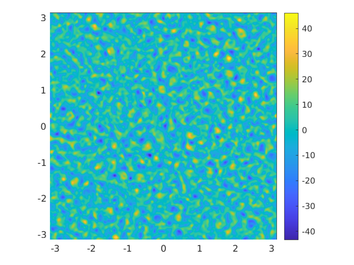
(a) Curl of initial velocity

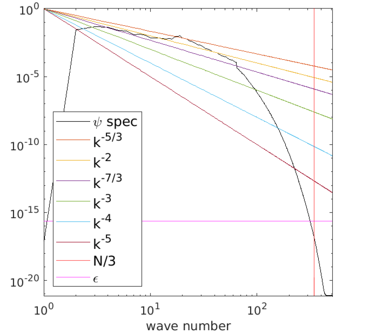
(b) Spectrum of initial $\psi$

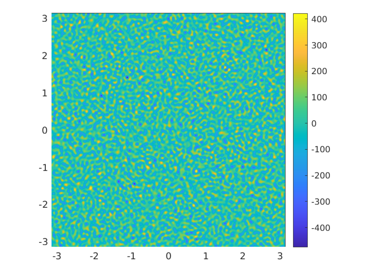
(c) Curl of the forcing

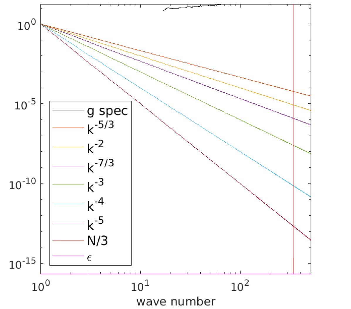
(d) Spectrum of curl of forcing

Figure 5.1. Initial data and forcing.

As for the forcing, in light of Remark 4.2, we were interested in a time-independent force which injects energy at high wave modes in order to better see the effect of the nonlinear-nudging data assimilation term (see 7.1 for further rationale). Therefore, we determined a forcing by choosing normally distributed random values for the real and complex part of each Fourier coefficient $\mathbf{f}_{\mathbf{k}}$ of the force with wavenumber between $16$ and $64$; namely, the set $\{\mathbf{k}=(k_{1},k_{2})|\,16^{2}\leq k_{1}^{2}$ $+k_{2}^{2}\leq 64^{2}\}$ (in fact, only half of the wavemodes were assigned and the rest were computed using the reality condition $\mathbf{f}_{-\mathbf{k}}=\overline{\mathbf{f}_{\mathbf{k}}}$). Matlab’s random number generator was initialized using rng(0) for consistency and reproducibility. The curl of the forcing, and its energy spectrum, are pictured in Figure 5.1.

Our parameters were chosen as follows: The Grashof number was $G=250,000$, the viscosity was $\nu=0.008$, and $h$ was chosen so that wavemodes of wavenumbers less than or equal to $32$ were observed; that is, the wavemodes at wavenumbers $\left\{\mathbf{k}=(k_{1},k_{2})|\,0<k_{1}^{2}+k_{2}^{2}\leq 32^{2}\right\}$ were observed. For the nonlinear-nudging data assimilation parameters, we choose $\gamma=0.1$, and $\mu=\beta=2$. These parameter ranges were not finely tuned to exhibit any special behavior, other than avoiding instability (seen, e.g., when $\mu$ is too large). In our own tests (data not reported here), we observed that modest changes in these parameter values did not yield significant qualitative changes in the results, indicating qualitative robustness of the results.

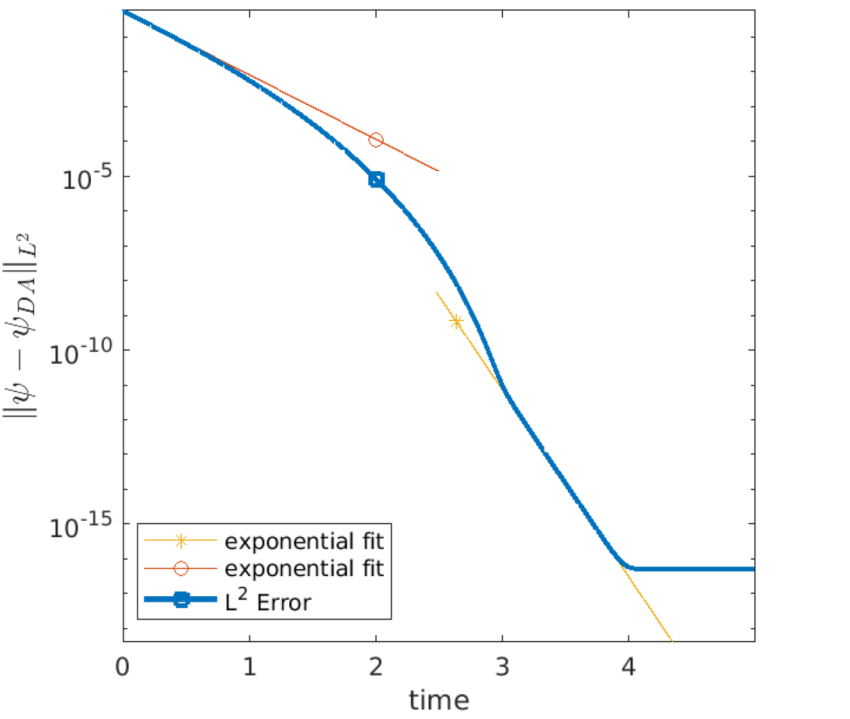
(a) (log-linear plot) Blue curve: $L^{2}$ error of the solution. Red line: Exponential fit up to time $t\approx 0.15$. Orange line: Exponential fit for $3.1\lesssim t\lesssim 3.8$.

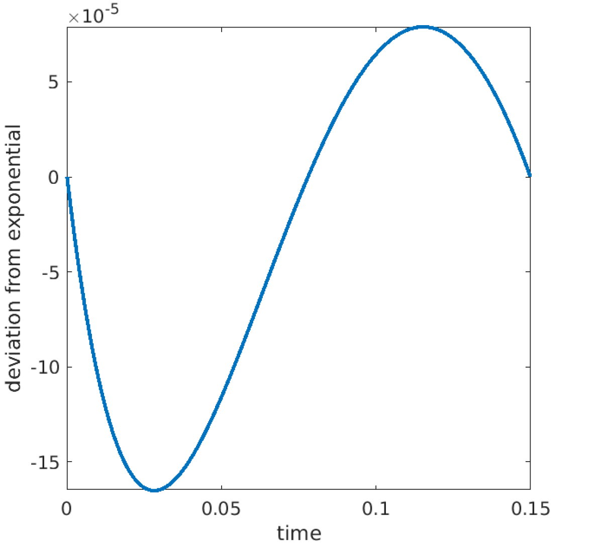
(b) (linear-linear plot) Error minus (red line) exponential fit.

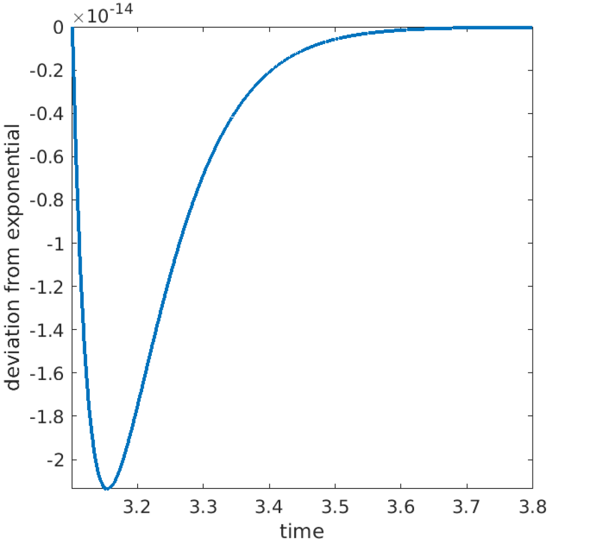
(c) (linear-linear plot) Error minus (orange line) exponential fit.

Figure 5.2. (A): $L^{2}$ error between the assimilated and true solutions. (B) and (C): deviations from exponential fits.

These graphics in particular corroborate our analysis in terms of the failing of super-exponential convergence due the $\epsilon$-barrier being reached, as seen in Figure 5.2. In particular, in Figure 2(a), convergence appears exponential at early times, then becomes super-exponential, and finally returns to merely exponential at later times. The deviations from an exponential fit was observed to be fairly small: $1.7\times 10^{-4}$ at early times (see Figure 2(b)) and $2.2\times 10^{-14}$ at later times. In between these times, super-exponential convergence is observed (see Figure 2(a)).

6. Conclusion

In this paper, we proved the existence of solutions to the nonlinear-nudging data assimilation system under the same assumptions on the interpolant as that of the linear-nudging data assimilation system. Uniqueness of solutions were proven to hold under more stringent assumptions on the interpolant operator of the observed measurements. With different assumptions on the interpolant, convergence of any corresponding solution to the nonlinear-nudging data assimilation to the true solution of the 2D incompressible Navier-Stokes equations was shown to be obtained up to a prescribed error in finite time at an at least double-exponential rate. In particular, any solution of the nonlinear-nudging system, even in regimes where uniqueness might not hold, will converge to the true solution. These results provide a theoretical foundation for the computational results seen in simulations in [61, 55], and the present work.

7. Appendix

7.1. Heuristic argument for the $\epsilon$-barrier

We analyze (1.3a) in the Navier-Stokes case (2.10), i.e., $\mathcal{F}(\mathbf{v})=-B(\mathbf{v},\mathbf{v})-\nu A\mathbf{v}+\mathbf{f}$, with $I_{h}=P_{m}$, i.e., projection onto the low Fourier modes of index $m<1/h$. This yields the equation

(7.1) $$\mathbf{v}_{t}+\nu A\mathbf{v}=B(\mathbf{v},\mathbf{v})-\mu\|P_{m}(\mathbf{u}-\mathbf{v})\|_{L^{2}(\Omega)}^{-\gamma}P_{m}(\mathbf{v}-\mathbf{u})-\beta P_{m}(\mathbf{v}-\mathbf{u})$$

Set $\mathbf{w}=\mathbf{v}-\mathbf{u}$. Subtracting (7.1) from the reference system, one obtains

(7.2) $$\mathbf{w}_{t}+\nu A\mathbf{w}=B(\mathbf{v},\mathbf{v})-B(\mathbf{u},\mathbf{u})-\mu\|P_{m}\mathbf{w}\|_{L^{2}(\Omega)}^{-\gamma}P_{m}\mathbf{w}-\beta P_{m}\mathbf{w}.$$

Taking a (formal) inner-product with $\mathbf{w}$ and simplifying yields

(7.3) $$\quad\frac{1}{2}\frac{d}{dt}\|\mathbf{w}\|_{L^{2}(\Omega)}^{2}+\nu\|A^{1/2}\mathbf{w}\|_{L^{2}(\Omega)}^{2}$$

$$=\left<B(\mathbf{v},\mathbf{v})-B(\mathbf{u},\mathbf{u}),\mathbf{w}\right>-\mu\|P_{m}\mathbf{w}\|^{-\gamma}\|P_{m}\mathbf{w}\|_{L^{2}(\Omega)}^{2}-\beta\|P_{m}\mathbf{w}\|_{L^{2}(\Omega)}^{2}.$$

Denoting $Q_{m}:=I-P_{m}$ and noting that $\|\mathbf{w}\|_{L^{2}}^{2}=\|P_{m}\mathbf{w}\|_{L^{2}}^{2}+\|Q_{m}\mathbf{w}\|_{L^{2}}^{2}$,

$$\quad\frac{1}{2}\frac{d}{dt}\|\mathbf{w}\|_{L^{2}(\Omega)}^{2}+\nu\|A^{1/2}\mathbf{w}\|_{L^{2}(\Omega)}^{2}+\beta\|\mathbf{w}\|_{L^{2}(\Omega)}^{2}+\mu\|P_{m}\mathbf{w}\|_{L^{2}(\Omega)}^{-\gamma}\|\mathbf{w}\|_{L^{2}(\Omega)}^{2}$$

$$=\left<B(\mathbf{v},\mathbf{v})-B(\mathbf{u},\mathbf{u}),\mathbf{w}\right>+\mu\|P_{m}\mathbf{w}\|_{L^{2}(\Omega)}^{-\gamma}\|Q_{m}\mathbf{w}\|_{L^{2}(\Omega)}^{2}+\beta\|Q_{m}\mathbf{w}\|_{L^{2}(\Omega)}^{2}$$

Rearranging, we obtain

(7.4) $$\quad\frac{1}{2}\frac{d}{dt}\|\mathbf{w}\|_{L^{2}(\Omega)}^{2}+\frac{\nu}{2}\|P_{m}A^{1/2}\mathbf{w}\|_{L^{2}(\Omega)}^{2}+\frac{\nu}{2}\|A^{1/2}\mathbf{w}\|_{L^{2}(\Omega)}^{2}$$

$$\quad+\beta\|\mathbf{w}\|_{L^{2}(\Omega)}^{2}+\mu\|P_{m}\mathbf{w}\|_{L^{2}(\Omega)}^{-\gamma}\|\mathbf{w}\|_{L^{2}(\Omega)}^{2}$$

$$=\left<B(\mathbf{v},\mathbf{v})-B(\mathbf{u},\mathbf{u}),\mathbf{w}\right>+\mu\|P_{m}\mathbf{w}\|_{L^{2}(\Omega)}^{-\gamma}\|Q_{m}\mathbf{w}\|_{L^{2}(\Omega)}^{2}$$

$$\quad+\beta\|Q_{m}\mathbf{w}\|_{L^{2}(\Omega)}^{2}-\frac{\nu}{2}\|Q_{m}A^{1/2}\mathbf{w}\|_{L^{2}(\Omega)}^{2}$$

We leave part of the dissipation on the left-hand side to absorb terms bounding $B(\mathbf{v},\mathbf{v})-B(\mathbf{u},\mathbf{u})$. The terms $\|Q_{m}\mathbf{w}\|_{L^{2}(\Omega)}^{2}$ and $\|Q_{m}\mathbf{w}\|_{L^{2}(\Omega)}^{2-\gamma}$ are the terms hindering the exponential convergence of $\mathbf{v}$ to the reference solution $\mathbf{u}$, and hence we want these last three terms to be negative overall. We expand the last three terms on the right-hand side to obtain

(7.5) $$\sum\limits_{|\mathbf{k}|=m+1}^{\infty}(\mu\|P_{m}\mathbf{w}\|_{L^{2}}^{-\gamma}+\beta-\frac{\nu}{2}|\mathbf{k}|^{2})|\hat{\mathbf{w}}_{\mathbf{k}}|^{2}\leq 0.$$

No matter how large one takes $m$ (i.e., how small $h$ is taken, since we generally take $m\sim L/h^{2}$, where $L$ is a characteristic length scale), as $\|\mathbf{w}\|_{L^{2}(\Omega)}\to 0$, $\|P_{m}\mathbf{w}\|_{L^{2}}^{-\gamma}\to\infty$, indicating there is a time at which the error becomes small enough that this term will hurt the rate of convergence rather than help. Moreover, we see from (7.4) that the larger $\beta$ is chosen (e.g., in order to enhance the convergence rate of the small scales), the more strongly the small scales (as measured by $\|Q_{m}\mathbf{w}\|_{L^{2}(\Omega)}^{2}$) are destabilized. This appears to be the reason why the super-exponential convergence rate is eventually destroyed, as seen both in our analysis and in our simulations. We refer to this as a “spill-over” effect; namely, the phenomenon that increased control of the large scales leads to increased destabilization of the small scales. In the case of the Navier-Stokes equations, the spill-over of energy into the small scales is controlled by the presence of viscosity; namely, for large enough $\nu$, the error in the small scales is damped strongly enough to counteract the spill-over effect.

Marvelously, in the Navier-Stokes case, the exponential convergence still holds in spite of the spill-over effect. This can be seen by writing (7.3) as

(7.6) $$\quad\frac{1}{2}\frac{d}{dt}\|\mathbf{w}\|_{L^{2}(\Omega)}^{2}+\nu\|A^{1/2}\mathbf{w}\|_{L^{2}(\Omega)}^{2}$$

$$=\left<B(\mathbf{v},\mathbf{v})-B(\mathbf{u},\mathbf{u}),\mathbf{w}\right>-(\beta+\mu)\|P_{m}\mathbf{w}\|_{L^{2}(\Omega)}^{2}+\mu(\|P_{m}\mathbf{w}\|_{L^{2}(\Omega)}^{2}-\|P_{m}\mathbf{w}\|_{L^{2}(\Omega)}^{2-\gamma});$$

the final term becomes negative as $\|\mathbf{w}\|_{L^{2}(\Omega)}\to 0$, and hence exponential convergence is maintained with an improved rate than for the standard linear-nudging CDA algorithm thanks to the added $\mu$ in the linear term. In other words, although the rate of convergence is no longer super exponential, the nonlinear-nudging term does not become so malicious as $\|\mathbf{w}\|_{L^{2}(\Omega)}\to 0$ that it counteracts the standard exponential convergence and in fact it still improves the exponential rate of convergence. This further elucidates our comments in Remark 4.6, i.e., an exponential rate of convergence can be maintained by the nonlinear-nudging term alone.

7.2. Proof of Lemma 2.7

Proof.

Let $\delta:=\min\left\{a/2,a^{\frac{2-\gamma}{2}}\left(\frac{\epsilon}{\left(\frac{2-\gamma}{2}\right)^{\frac{2-\gamma}{\gamma}}-\left(\frac{2-\gamma}{2}\right)^{\frac{2}{\gamma}}}\right)^{\frac{\gamma}{2}}\right\}$. Note that $f(x)$ has two critical points at $x=0$ and $x=\left(\frac{(2-\gamma)\delta}{2a}\right)^{\frac{1}{\gamma}}$. We further note that $f(x_{0})$ is a global minimum since $f(0)=0$,

$$f(x_{0}) =a\left(\left(\frac{(2-\gamma)\delta}{2a}\right)^{\frac{1}{\gamma}}\right)^{2}-\delta\left(\left(\frac{(2-\gamma)\delta}{2a}\right)^{\frac{1}{\gamma}}\right)^{2-\gamma}$$

$$=a^{-\frac{2-\gamma}{\gamma}}\delta^{\frac{2}{\gamma}}\left(\left(\frac{2-\gamma}{2}\right)^{\frac{2}{\gamma}}-\left(\frac{2-\gamma}{2}\right)^{\frac{2-\gamma}{\gamma}}\right)\leq 0,$$

$f^{\prime}(x)\geq 0$ for all $x\geq x_{0}$, and $f^{\prime}(x)\leq 0$ for $x\leq x_{0}$. Indeed, $f^{\prime}(x)\geq 0$ for all $x\geq x_{0}$ since

$$f^{\prime}(x) \geq 2ax-(2-\gamma)\delta x_{0}^{1-\gamma}$$

$$=2ax-(2-\gamma)\delta\left(\frac{(2-\gamma)\delta}{2a}\right)^{\frac{1-\gamma}{\gamma}}$$

$$=2a\left(x-\left(\frac{(2-\gamma)\delta}{2a}\right)^{\frac{1}{\gamma}}\right)$$

$$=2a(x-x_{0})$$

$$\geq 0,$$

and $f^{\prime}(x)\leq 0$ for all $x\leq x_{0}$ since

$$f^{\prime}(x) \leq 2ax_{0}-(2-\gamma)\delta x^{1-\gamma}$$

$$=2a\left(\frac{(2-\gamma)\delta}{2a}\right)^{\frac{1}{\gamma}}-(2-\gamma)\delta x^{1-\gamma}$$

$$=(2-\gamma)\delta(\left(\frac{(2-\gamma)\delta}{2a}\right)^{\frac{1-\gamma}{\gamma}}-x^{1-\gamma})$$

$$=(2-\gamma)\delta(x_{0}^{1-\gamma}-x^{1-\gamma})$$

$$\leq 0.$$

Hence, $f(x)\geq f(x_{0})$ for all $x\in\mathbb{R}_{\geq 0}$. Thus, denoting

$$b:=\left(\left(\frac{2-\gamma}{2}\right)^{\frac{2-\gamma}{\gamma}}-\left(\frac{2-\gamma}{2}\right)^{\frac{2}{\gamma}}\right),$$

our choice of $\delta$ yields

$$f(x)\geq f(x_{0}) \geq a^{-\frac{2-\gamma}{\gamma}}\left(a^{\frac{2-\gamma}{2}}\left(\frac{\epsilon}{b}\right)^{\frac{\gamma}{2}}\right)^{\frac{2}{\gamma}}(-b)=-\epsilon.$$

∎

7.3. Computation of explicit times at which the nonlinear-nudging term in the algorithm improves the convergence rate

Note that one can compute a time $t_{a}$ at which $\mathbf{u}$ is in the absorbing ball (see, e.g. [44, 75, 78]) so that Theorem 2.3 applies and the exponential decay in [4] holds. The decay of the nonlinear-nudging algorithm is controlled by the exponential decay of the linear-nudging algorithm in [4] (see the beginning of the proofs of Theorems 4.1,4.4) can be written explicitly as (for reference, see, e.g., [18])

$$\|\mathbf{u}(t)-\mathbf{v}(t)\|_{H}^{2} \leq\|\mathbf{u}(t_{a})-\mathbf{v}(t_{a})\|_{H}^{2}e^{1+r/2}e^{-\frac{r}{2T}(t-t_{a})},$$

where $\frac{1}{\nu\lambda_{1}}<T<\infty$ and

$$r =\liminf\limits_{t\to\infty}\int_{t}^{t+T}\beta-\frac{2c^{2}}{\nu}\|\mathbf{u}(s)\|^{2}ds$$

$$\geq T\beta-\frac{2c^{2}}{\nu}\left(2(1+\lambda_{1}T\nu)\nu G^{2}\right)>0,$$

and $c$ is the constant from the inequality (2.6).

By the assumptions of Theorem 4.1, we need that $\|\mathbf{u}(t_{0})-\mathbf{v}(t_{0})\|_{H}<R_{H}$, where $R_{H}=\min\left\{e^{-\frac{1}{\beta\gamma\lambda_{1}^{\gamma/2}}},\left(\frac{\beta\lambda_{1}^{\gamma/2}}{\beta\lambda_{1}^{\gamma/2}+1}\right)^{1/\gamma}\right\}$, so we need to choose $t_{a}$ such that

$$\|\mathbf{u}(t_{a})-\mathbf{v}(t_{a})\|_{H}^{2}e^{1+r/2}e^{-\frac{r}{2T}(t-t_{a})}<R_{H}^{2}.$$

Bounding $\|\mathbf{u}(t_{a})\|_{H}^{2}$ using Theorem 2.3 and using the bounds on $r$, we instead find a time $t_{a}$ such that

$$\|\mathbf{u}(t_{a}) -\mathbf{v}(t_{a})\|_{H}^{2}e^{1+r/2}e^{-\frac{r}{2T}(t-t_{a})}$$

$$\leq 2(2(\nu)^{2}G^{2}+\|\mathbf{v}(t_{a})\|_{H}^{2})e^{1+\beta T}e^{-\beta/2-\frac{c^{2}}{\nu T}(2(1+\lambda_{1}T\beta)\nu G^{2})(t-t_{a})}$$

$$<R_{H}^{2}.$$

Thus, we determine the nonlinear-nudging system can be initialized from any time $t_{0}$ such that

$$t_{0}>t_{a}-\frac{\log\left\{\frac{R_{H}^{2}e^{-1-\beta T}}{2(2(\nu)^{2}G^{2}+\|\mathbf{v}(t_{a})\|_{H}^{2})}\right\}}{\beta/2-\frac{c^{2}}{T\nu}(2(1+\lambda_{1}\nu T)\nu G^{2})}.$$

There is no need to observe $\|\mathbf{v}(t_{a})\|_{H}$ at the fixed time $t_{a}$; instead, the bound from [4]

$$\|\mathbf{v}(t_{a})\|_{H}^{2}\leq e^{-\nu\lambda_{1}t_{a}}\|\mathbf{v}_{0}\|_{H}^{2}+\frac{M}{\beta\nu\lambda_{1}}(1-e^{-\nu\lambda t_{a}}):=\text{RHS}_{H},$$

where $M$ is a constant such that $\|f+\beta P_{\sigma}I_{h}(\mathbf{w}))\|_{H}^{2}<M$, can be used to choose a time $t_{0}$ such that

$$t_{0}>t_{a}-\frac{\log\left\{\frac{R_{H}^{2}e^{-1-\beta T}}{2(2(\nu)^{2}G^{2}+\text{RHS}_{H})})\right\}}{\beta/2-\frac{c^{2}}{T\nu}(2(1+\lambda_{1}\nu T)\nu G^{2})}.$$

For the setting of Theorem 4.4, we have the bound

$$\|\mathbf{u}(t)-\mathbf{v}(t)\|_{V}^{2} \leq\|\mathbf{u}(t_{a})-\mathbf{v}(t_{a})\|^{2}e^{\Gamma+1+r/2}e^{-\frac{r}{2T}(t-t_{a})},$$

where $\lambda_{1}\nu\leq T<\infty$,

$$r=\liminf\limits_{t\to\infty}\int_{t}^{t+T}\frac{1}{2}\left(\beta-\frac{J^{2}}{\beta}\|A\mathbf{u}\|_{H}^{2}\right)ds>\frac{5}{6}JG>0,$$

and

$$\Gamma=\liminf\limits_{t\to\infty}\int_{t}^{t+T}\max\left\{\frac{1}{2}\left(\beta-\frac{J^{2}}{\beta}\|A\mathbf{u}\|_{H}^{2}\right),0\right\}ds\geq r>0,$$

with $J=2c\log(2c^{3/2})+4c\log(1+G)$ and $c$ is the constant dependent on the domain determined from the Brezis-Gallouet inequality. By the assumptions of Theorem 4.4, we need that $\|\mathbf{u}(t_{0})-\mathbf{v}(t_{0})\|_{V}<R_{V}$, where $R_{V}=\min\left\{e^{-\frac{1}{\beta\gamma\lambda_{1}^{\gamma/2}}},\left(\frac{\beta\lambda_{1}^{\gamma/2}}{\beta\lambda_{1}^{\gamma/2}+1}\right)^{1/\gamma}\right\}$, so we need to choose $t_{0}$ such that

$$\|\mathbf{u}(t_{a})-\mathbf{v}(t_{a})\|_{V}^{2}e^{\Gamma+1+r/2}e^{-\frac{r}{2T}(t-t_{a})}<R_{V}^{2}.$$

Again, bounding $\|\mathbf{u}(t_{a})\|_{V}^{2}$ using Theorem 2.3 and using the bounds on $\Gamma$ and $r$, we instead find a time $t_{a}$ such that

$$\|\mathbf{u}(t_{a}) -\mathbf{v}(t_{a})\|_{V}^{2}e^{\Gamma+1+r/2}e^{-\frac{r}{2T}(t-t_{a})}$$

$$\leq 2(2\lambda_{1}(\nu)^{2}G^{2}+\|\mathbf{v}(t_{a})\|^{2})e^{1+\beta T}e^{-\frac{5}{6}GJ(t-t_{a})}<R_{V}^{2}$$

Then, the nonlinear-nudging system can be initialized from any time $t_{0}$ such that

$$t_{0}>t_{a}-\frac{6}{5GJ}\log\left\{\frac{R_{V}^{2}e^{-(1+\beta T)}}{2(2\lambda_{1}(\nu)^{2}G^{2}+\|\mathbf{v}(t_{a})\|_{V}^{2})}\right\}.$$

Again, there is no need to observe $\|\mathbf{v}(t_{a})\|_{V}$ at the fixed time $t_{a}$, since the bound from [4]

$$\quad\|\mathbf{v}(t_{a})\|_{V}^{2}\leq\text{RHS}_{V}$$

$$:=e^{\frac{54c^{4}}{(\nu)^{3}}\left(\frac{1}{\nu}\|\mathbf{v}_{0}\|_{H}^{2}+\frac{T}{\nu\beta}M\right)^{2}\left(\frac{1}{\nu}\|\mathbf{v}_{0}\|_{V}^{2}+\frac{M}{\beta\nu\lambda_{1}}\right)^{2}}\left(\|\mathbf{v}_{0}\|_{V}^{2}+\frac{4T}{\nu}M\right)$$

where $M$ is the same constant such that $\|f+\beta P_{\sigma}I_{h}(\mathbf{w}))\|_{H}^{2}<M$, can be used to choose a time $t_{0}$ such that

$$t_{0}>t_{a}-\frac{6}{5GJ}\log\left\{\frac{R_{V}^{2}e^{-(1+\beta T)}}{2\left(2\lambda_{1}(\nu)^{2}G^{2}+\text{RHS}_{V}\right)}\right\}.$$

References

• [1] M. Akbas and A. Çibik. Continuous data assimilation for double-diffusive natural convection. arXiv: 2008.02224, 2020.
• [2] D. A. Albanez, H. J. Nussenzveig Lopes, and E. S. Titi. Continuous data assimilation for the three-dimensional Navier–Stokes-$\alpha$ model. Asymptotic Anal., 97(1-2):139–164, 2016.
• [3] M. U. Altaf, E. S. Titi, O. M. Knio, L. Zhao, M. F. McCabe, and I. Hoteit. Downscaling the 2D Benard convection equations using continuous data assimilation. Comput. Geosci, 21(3):393–410, 2017.
• [4] A. Azouani, E. Olson, and E. S. Titi. Continuous data assimilation using general interpolant observables. J. Nonlinear Sci., 24(2):277–304, 2014.
• [5] A. Azouani and E. S. Titi. Feedback control of nonlinear dissipative systems by finite determining parameters—a reaction-diffusion paradigm. Evol. Equ. Control Theory, 3(4):579–594, 2014.
• [6] A. Balakrishna and A. Biswas. Determining map, data assimilation and an observable regularity criterion for the three-dimensional Boussinesq system. Appl Math Optim, 86, 2022.
• [7] C. Basdevant. Technical improvements for direct numerical simulation of homogeneous three-dimensional turbulence. J. Comput. Phys., 50(2):209–214, 1983.
• [8] H. Bessaih, V. Ginting, and B. McCaskill. Continuous data assimilation for displacement in a porous medium. Numer. Math., 151:927–962, 2022.
• [9] H. Bessaih, E. Olson, and E. S. Titi. Continuous data assimilation with stochastically noisy data. Nonlinearity, 28(3):729–753, 2015.
• [10] A. Biswas, Z. Bradshaw, and M. S. Jolly. Data assimilation for the Navier–Stokes equations using local observables. SIAM Journal on Applied Dynamical Systems, 20(4):2174–2203, 2021.
• [11] A. Biswas, C. Foias, C. F. Mondaini, and E. S. Titi. Downscaling data assimilation algorithm with applications to statistical solutions of the Navier–Stokes equations. In Annales de l’Institut Henri Poincaré C, Analyse non linéaire, pages 295–326. Elsevier, 2019.
• [12] A. Biswas, J. Hudson, A. Larios, and Y. Pei. Continuous data assimilation for the 2D magnetohydrodynamic equations using one component of the velocity and magnetic fields. Asymptot. Anal., 108(1-2):1–43, 2018.
• [13] A. Biswas and V. R. Martinez. Higher-order synchronization for a data assimilation algorithm for the 2D Navier–Stokes equations. Nonlinear Anal. Real World Appl., 35:132–157, 2017.
• [14] A. Biswas and R. Price. Continuous data assimilation for the three-dimensional Navier–Stokes equations. SIAM Journal on Mathematical Analysis, 53(6):6697–6723, 2021.
• [15] S. Brenner and L. R. Scott. The Mathematical Theory of Finite Element Methods. Texts in Applied Mathematics. Springer, 2008.
• [16] C. Cao, I. G. Kevrekidis, and E. S. Titi. Numerical criterion for the stabilization of steady states of the Navier–Stokes equations. Indiana Univ. Math. J., 50(Special Issue):37–96, 2001. Dedicated to Professors Ciprian Foias and Roger Temam (Bloomington, IN, 2000).
• [17] Y. Cao, A. Giorgini, M. Jolly, and A. Pakzad. Continuous data assimilation for the 3D Ladyzhenskaya model: Analysis and computations. Nonlinear Anal. Real World Appl., 68, 2022.
• [18] E. Carlson, J. Hudson, and A. Larios. Parameter recovery for the 2 dimensional Navier-Stokes equations via continuous data assimilation. SIAM J. Sci. Comput., 42(1):A250–A270, 2020.
• [19] E. Carlson, J. Hudson, A. Larios, V. R. Martinez, E. Ng, and J. Whitehead. Dynamically learning the parameters of a chaotic system using partial observations. Discrete Contin Dyn Syst Ser A, 42(8):3809–3839, 2022.
• [20] E. Carlson and A. Larios. Sensitivity analysis for the 2D Navier-Stokes equations with applications to continuous data assimilation. J. Nonlinear Sci., 31(5):Paper No. 84, 30, 2021.
• [21] E. Carlson, L. Van Roekel, M. Petersen, H. C. Godinez, and A. Larios. CDA algorithm implemented in MPAS-O to improve eddy effects in a mesoscale simulation. 2023. (submitted).
• [22] E. Celik, E. Olson, and E. S. Titi. Spectral filtering of interpolant observables for a discrete-in-time downscaling data assimilation algorithm. SIAM J. Appl. Dyn. Syst., 18(2):1118–1142, 2019.
• [23] N. Chen, Y. Li, and E. Lunasin. An efficient continuous data assimilation algorithm for the sabra shell model of turbulence. Chaos, 31(10):103123, 2021.
• [24] Y. T. Chow, W. T. Leung, and A. Pakzad. Continuous data assimilation for two-phase flow: Analysis and simulations. Journal of Computational Physics, 466:111395, 2022.
• [25] P. Clark Di Leoni, A. Mazzino, and L. Biferale. Inferring flow parameters and turbulent configuration with physics-informed data assimilation and spectral nudging. Phys. Rev. Fluids, 3(10):104604, 2018.
• [26] B. Cockburn, D. Jones, and E. S. Titi. Estimating the number of asymptotic degrees of freedom for nonlinear dissipative systems. Math. Comput., 66(219):1073–1087, 1997.
• [27] P. Constantin and C. Foias. Navier–Stokes Equations. Chicago Lectures in Mathematics. University of Chicago Press, Chicago, IL, 1988.
• [28] J. B. Conway. A Course in Functional Analysis, volume 96 of Graduate Texts in Mathematics. Springer-Verlag, New York, second edition, 1990.
• [29] R. Dascaliuc, C. Foias, and M. S. Jolly. Estimates on enstrophy, palinstrophy, and invariant measures for 2-D turbulence. J. Differential Equations, 248(4):792–819, 2010.
• [30] S. Desamsetti, H. Dasari, S. Langodan, O. Knio, I. Hoteit, and E. S. Titi. Efficient dynamical downscaling of general circulation models using continuous data assimilation. Quarterly Journal of the Royal Meteorological Society, 2019.
• [31] S. Desamsetti, H. P. Dasari, S. Langodan, Y. Viswanadhapalli, R. Attada, T. M. Luong, O. Knio, E. S. Titi, and I. Hoteit. Enhanced simulation of the Indian summer monsoon rainfall using regional climate modeling and continuous data assimilation. Frontiers in Climate, 4, 2022.
• [32] A. E. Diegel and L. G. Rebholz. Continuous data assimilation and long-time accuracy in a $\rm C^{0}$ interior penalty method for the Cahn-Hilliard equation. Appl. Math. Comput., 424:Paper No. 127042, 22, 2022.
• [33] Y. J. Du and M.-C. Shiue. Analysis and computation of continuous data assimilation algorithms for Lorenz 63 system based on nonlinear nudging techniques. J. Comput. Appl. Math., 386:113246, 2021.
• [34] P. Emami and J. C. Bowman. On the global attractor of 2D incompressible turbulence with random forcing. J. Differential Equations, 264(6):4036–4066, 2018.
• [35] L. C. Evans. Partial Differential Equations, volume 19 of Graduate Studies in Mathematics. American Mathematical Society, Providence, RI, second edition, 2010.
• [36] A. Farhat, N. E. Glatt-Holtz, V. R. Martinez, S. A. McQuarrie, and J. P. Whitehead. Data assimilation in large Prandtl Rayleigh–Bénard convection from thermal measurements. SIAM J. Appl. Dyn. Syst., 19(1):510–540, 2020.
• [37] A. Farhat, H. Johnston, M. Jolly, and E. S. Titi. Assimilation of nearly turbulent Rayleigh–Bénard flow through vorticity or local circulation measurements: A computational study. Journal of Scientific Computing, 77(3):1519–1533, Dec 2018.
• [38] A. Farhat, M. S. Jolly, and E. S. Titi. Continuous data assimilation for the 2D Bénard convection through velocity measurements alone. Phys. D, 303:59–66, 2015.
• [39] A. Farhat, E. Lunasin, and E. S. Titi. Abridged continuous data assimilation for the 2D Navier–Stokes equations utilizing measurements of only one component of the velocity field. J. Math. Fluid Mech., 18(1):1–23, 2016.
• [40] A. Farhat, E. Lunasin, and E. S. Titi. Data assimilation algorithm for 3D Bénard convection in porous media employing only temperature measurements. J. Math. Anal. Appl., 438(1):492–506, 2016.
• [41] A. Farhat, E. Lunasin, and E. S. Titi. On the Charney conjecture of data assimilation employing temperature measurements alone: the paradigm of 3D planetary geostrophic model. Mathematics of Climate and Weather Forecasting, 2(1), 2016.
• [42] A. Farhat, E. Lunasin, and E. S. Titi. Continuous data assimilation for a 2D Bénard convection system through horizontal velocity measurements alone. J. Nonlinear Sci., pages 1–23, 2017.
• [43] A. Farhat, E. Lunasin, and E. S. Titi. A data assimilation algorithm: the paradigm of the 3D Leray-$\alpha$ model of turbulence. Partial differential equations arising from physics and geometry, 450:253–273, 2019.
• [44] C. Foias, O. Manley, R. Rosa, and R. Temam. Navier–Stokes Equations and Turbulence, volume 83 of Encyclopedia of Mathematics and its Applications. Cambridge University Press, Cambridge, 2001.
• [45] C. Foias, C. F. Mondaini, and E. S. Titi. A discrete data assimilation scheme for the solutions of the two-dimensional Navier–Stokes equations and their statistics. SIAM J. Appl. Dyn. Syst., 15(4):2109–2142, 2016.
• [46] K. Foyash, M. S. Dzholli, R. Kravchenko, and È. S. Titi. A unified approach to the construction of defining forms for a two-dimensional system of Navier–Stokes equations: the case of general interpolating operators. Uspekhi Mat. Nauk, 69(2(416)):177–200, 2014.
• [47] T. Franz, A. Larios, and C. Victor. The bleeps, the sweeps, and the creeps: Convergence rates for dynamic observer patterns via data assimilation for the 2D Navier-Stokes equations. Comput. Methods Appl. Mech. Engrg., 392:Paper No. 114673, 19, 2022.
• [48] B. García-Archilla and J. Novo. Error analysis of fully discrete mixed finite element data assimilation schemes for the Navier-Stokes equations. Adv. Comput. Math., 46(4):Paper No. 61, 33, 2020.
• [49] B. García-Archilla, J. Novo, and E. S. Titi. Uniform in time error estimates for a finite element method applied to a downscaling data assimilation algorithm for the Navier-Stokes equations. SIAM J. Numer. Anal., 58(1):410–429, 2020.
• [50] M. Gardner, A. Larios, L. G. Rebholz, D. Vargun, and C. Zerfas. Continuous data assimilation applied to a velocity-vorticity formulation of the 2D Navier-Stokes equations. Electron. Res. Arch., 29(3):2223–2247, 2021.
• [51] M. Germano. Blending and nudging in fluid dynamics: some simple observations. Fluid Dynamics Research, 49(5):055503, aug 2017.
• [52] M. Gesho, E. Olson, and E. S. Titi. A computational study of a data assimilation algorithm for the two-dimensional Navier–Stokes equations. Commun. Comput. Phys., 19(4):1094–1110, 2016.
• [53] N. Glatt-Holtz, I. Kukavica, V. Vicol, and M. Ziane. Existence and regularity of invariant measures for the three dimensional stochastic primitive equations. J. Math. Phys., 55(5):051504, 34, 2014.
• [54] K. Hayden, E. Olson, and E. S. Titi. Discrete data assimilation in the Lorenz and 2D Navier–Stokes equations. Phys. D, 240(18):1416–1425, 2011.
• [55] J. Hudson and M. Jolly. Numerical efficacy study of data assimilation for the 2D magnetohydrodynamic equations. J. Comput. Dyn., 6(1):131–145, 2019.
• [56] H. A. Ibdah, C. F. Mondaini, and E. S. Titi. Fully discrete numerical schemes of a data assimilation algorithm: uniform-in-time error estimates. IMA Journal of Numerical Analysis, 40(4):2584–2625, 2020.
• [57] M. S. Jolly, V. R. Martinez, E. J. Olson, and E. S. Titi. Continuous data assimilation with blurred-in-time measurements of the surface quasi-geostrophic equation. Chin. Ann. Math. Ser. B, 40(5):721–764, 2019.
• [58] M. S. Jolly, V. R. Martinez, and E. S. Titi. A data assimilation algorithm for the subcritical surface quasi-geostrophic equation. Adv. Nonlinear Stud., 17(1):167–192, 2017.
• [59] D. A. Jones and E. S. Titi. Upper bounds on the number of determining modes, nodes, and volume elements for the Navier-Stokes equations. Indiana Univ. Math. J., 42(3):875–887, 1993.
• [60] A.-K. Kassam and L. N. Trefethen. Fourth-order time-stepping for stiff PDEs. SIAM J. Sci. Comput., 26(4):1214–1233, 2005.
• [61] A. Larios and Y. Pei. Nonlinear continuous data assimilation. (submitted) arXiv:1703.03546.
• [62] A. Larios and Y. Pei. Approximate continuous data assimilation of the 2D Navier-Stokes equations via the Voigt-regularization with observable data. Evol. Equ. Control Theory, 9(3):733–751, 2020.
• [63] A. Larios, L. G. Rebholz, and C. Zerfas. Global in time stability and accuracy of IMEX-FEM data assimilation schemes for Navier-Stokes equations. Comput. Methods Appl. Mech. Engrg., 345:1077–1093, 2019.
• [64] A. Larios and C. Victor. Continuous data assimilation with a moving cluster of data points for a reaction diffusion equation: a computational study. Commun. Comput. Phys., 29(4):1273–1298, 2021.
• [65] E. Lunasin and E. S. Titi. Finite determining parameters feedback control for distributed nonlinear dissipative systems—a computational study. Evol. Equ. Control Theory, 6(4):535–557, 2017.
• [66] P. A. Markowich, E. S. Titi, and S. Trabelsi. Continuous data assimilation for the three-dimensional Brinkman-Forchheimer-extended Darcy model. Nonlinearity, 29(4):1292–1328, 2016.
• [67] V. R. Martinez. Convergence analysis of a viscosity parameter recovery algorithm for the 2D Navier–Stokes equations. Nonlinearity, 35(5):2241–2287, 2022.
• [68] V. R. Martinez. On the reconstruction of unknown driving forces from low-mode observations in the 2D Navier–Stokes equations. arXiv, 2022.
• [69] C. F. Mondaini and E. S. Titi. Uniform-in-time error estimates for the postprocessing Galerkin method applied to a data assimilation algorithm. SIAM J. Numer. Anal., 56(1):78–110, 2018.
• [70] E. Olson and E. S. Titi. Determining modes for continuous data assimilation in 2D turbulence. J. Statist. Phys., 113(5-6):799–840, 2003. Progress in statistical hydrodynamics (Santa Fe, NM, 2002).
• [71] E. Olson and E. S. Titi. Determining modes and grashof number in 2D turbulence: a numerical case study. Theor. Comp. Fluid Dyn., 22(5):327–339, 2008.
• [72] B. Pachev, J. P. Whitehead, and S. A. McQuarrie. Concurrent multi-parameter learning demonstrated on the Kuramoto–Sivashinsky equation. SIAM J. Sci. Comput., 44(5):A2974–A2990, 2022.
• [73] Y. Pei. Continuous data assimilation for the 3D primitive equations of the ocean. Commun. Pure Appl. Anal., 18(2):643–661, 2019.
• [74] L. G. Rebholz and C. Zerfas. Simple and efficient continuous data assimilation of evolution equations via algebraic nudging. Numer. Methods Partial Differ. Equations, pages 1–25, 2021.
• [75] J. C. Robinson. Infinite-Dimensional Dynamical Systems. Cambridge Texts in Applied Mathematics. Cambridge University Press, Cambridge, 2001. An Introduction to Dissipative Parabolic PDEs and the Theory of Global Attractors.
• [76] S. S. Rodrigues. Semiglobal oblique projection exponential dynamical observers for nonautonomous semilinear parabolic-like equations. J Nonlinear Sci, 31, 2021.
• [77] R. Temam. Navier–Stokes Equations and Nonlinear Functional Analysis, volume 66 of CBMS-NSF Regional Conference Series in Applied Mathematics. Society for Industrial and Applied Mathematics (SIAM), Philadelphia, PA, second edition, 1995.
• [78] R. Temam. Navier–Stokes Equations: Theory and Numerical Analysis. AMS Chelsea Publishing, Providence, RI, 2001. Theory and numerical analysis, Reprint of the 1984 edition.
• [79] E. S. Titi and S. Trabelsi. Global well-posedness of a three-dimensional Brinkman-Forchheimer-Bénard convection model in porous media. arXiv: Analysis of PDEs, 2022.
• [80] X. M. Wang. A remark on the characterization of the gradient of a distribution. Appl. Anal., 51(1-4):35–40, 1993.
• [81] B. You. A discrete data assimilation algorithm for the three dimensional planetary geostrophic equations of large-scale ocean circulation. J. Dyn. Differ. Equ., 2022.
• [82] B. You and Q. Xia. Continuous data assimilation algorithm for the two dimensional Cahn–Hilliard–Navier–Stokes system. Appl Math Optim, 85, 2022.
• [83] M. Zauner, V. Mons, O. Marquet, and B. Leclaire. Nudging-based data assimilation of the turbulent flow around a square cylinder. Journal of Fluid Mechanics, 937:A38, 2022.
• [84] C. Zerfas, L. G. Rebholz, M. Schneier, and T. Iliescu. Continuous data assimilation reduced order models of fluid flow. Comput. Methods Appl. Mech. Engrg., 357:112596, 18, 2019.