Port-Hamiltonian Modelling for Analysis and Control of Gas Networks

Abstract

In this paper, we present finite-dimensional port-Hamiltonian system (PHS) models of a gas pipeline and a network comprising several pipelines for the purpose of control design and stability analysis. Starting from the partial differential Euler equations describing the dynamical flow of gas in a pipeline, the method of lines is employed to obtain a lumped-parameter model, which simplifies to a nonlinear third-order PHS. Parallels between gas networks and power systems are drawn by showing that the obtained pipeline PHS model has the same $\pi$-representation as electrical transmission lines. Moreover, to assist future control design, additional passivity properties of the pipeline PHS model are analysed and discussed. By comparing the proposed PHS models against other models in a standard simulation, we show that the simplifying assumptions have no material effect on the model fidelity. The proposed pipeline and network models can serve as a basis for passivity-based control and analysis while the power system parallels facilitate the transfer of existing methods.

sm#1-+

1 Introduction

The combination of power to gas (P2G) facilities and the generation of green hydrogen envisions a sustainable and carbon-free future for gas networks. Since such P2G and electrolysis facilities are ideally supplied by excess renewable energy, the supply of gas from such facilities are also subject to the intermittency and volatility associated with e.g. solar and wind power. Additionally, gas-fired electricity and heat generation is increasingly being used to compensate intermittent electrical energy generation, which can cause pressure fluctuations (see Osiadacz and Chaczykowski (2020)). Due to the expected decrease in the overall demand for gas (see e.g. Qadrdan et al. (2019)), a coordination of the P2G facilities, local gas storages, flexible consumers and compressors supplying higher pressure networks will be required in the future.

For the control and subsequent stability analysis of such future gas networks, dynamical gas network models are required. Specifically, dynamical models are required for the pipelines, which are the most numerous components and typically exhibit the slowest dynamics. The flow of gas in the pipelines can accurately be described by the partial differential equations comprising the Euler equations. However, these PDEs pose a barrier to the application of many control and stability analysis methods applicable only to ordinary differential equations.

Literature Review

Herrán-González et al. (2009) andPambour et al. (2016) propose detailed simulation models for gas pipelines based on discretization. Similarly, Wiid et al. (2020) derive a nonlinear state-space model using the spectral element method for a pipeline with zero inclination. While the numerical nature of these models are appropriate for certain control methods (e.g. model predictive control), they generally provide no clear guidance towards control design or analytical system analysis. Ke and Ti (2000) and Taherinejad et al. (2017) provide pipeline models for control design and analysis inspired by electrical analogies, although the assumptions made significantly affect the model fidelity in comparison with e.g. the simulation model in Pambour et al. (2016). Furthermore, Alamian et al. (2012) propose a linearised state-space model and Zhou et al. (2017) presents linearised transfer functions for the pipeline dynamics. While the standard control and stability analysis methods can be applied to these linear models, the linearisation significantly impacts model accuracy. Finally, Domschke et al. (2021) propose various port-Hamiltonian-based models for a gas pipeline. PHS models may readily be used in passivity-based control and analysis methods without compromising model quality by removing nonlinear effects. Nevertheless, the infinite dimensional PHS models presented by Domschke et al. (2021) retain the PDE nature of the Euler equations, limiting their access to more general control and stability analysis methods in comparison to finite dimensional PHSs.

Main Contribution

In this paper, we propose finite dimensional PHS models for a gas pipeline and a network of gas pipelines for which standard control and analysis techniques can be applied. Specifically, this comprises:

1. A third order PHS model with a $\pi$-model structure similar to those of power system transmission lines.

2. A combined PHS model for an entire network of pipes.

3. A simulation demonstrating the fidelity of the proposed PHS model compared to other models.

Through parallels with models used for power systems and due to the use of the PHS framework, the proposed models provide a gateway for transferring established control and analysis methods in the field of power systems to the domain of gas networks. Moreover, we further facilitate such a transfer of established methods by highlighting certain passivity properties of the PHS models.

Paper Organisation

The introduction concludes with some notation and preliminaries. In Section 2, the equations representing the dynamics of an inclined gas pipeline are recalled. Next, in Section 3, PHS models are constructed for a gas pipeline and a network of pipelines. Thereafter in Section 4, the fidelity of the proposed PHS model is evaluated through a comparison with other pipeline models. Concluding remarks are supplied in Section 5.

Notation and Preliminaries

Define as a vector $\bm{a}=(a_{i})$ and a matrix $\bm{A}=(a_{ij})$. $\bm{\mathds{1}}_{k}$ is a $k$-dimensional vector of ones and $\bm{I}_{k}$ is the identity matrix of dimension $k$. $\mathbb{R}$ and $\mathbb{R}_{+}$ denote the real and positive real sets, respectively. $\operatorname{Diag}[\cdot]$ creates a (block-)diagonal matrix from the supplied vectors (or matrices). Note that we omit variable dependencies where clear from context. We denote by $\mathcal{G}=(\mathcal{V},\mathcal{E})$ a finite, undirected graph with vertices $\mathcal{V}$ and edges $\mathcal{E}\subseteq\mathcal{V}\times\mathcal{V}$. Let $|\mathcal{V}|$ be the cardinality of the set $\mathcal{V}$. By arbitrarily assigning directions to each edge in $\mathcal{E}$, the incidence matrix $\bm{B}\in\mathbb{R}^{|\mathcal{V}|\times|\mathcal{E}|}$ of $\mathcal{G}$ is defined by

$$b_{ij}=\left\{\begin{array}[]{@{}rl}+1&\text{if vertex $i$ is the sink of edge $j$},\\ -1&\text{if vertex $i$ is the source of edge $j$},\\ 0&\text{otherwise}.\end{array}\right.$$ (1)

2 Gas Pipeline Preliminaries

Figure 1: A gas pipeline sectioned into a left and a right side, superimposed with its electrical equivalent circuit.

In this section, we briefly recall the equations governing the flow of gas in an inclined pipeline (see Fig. 1). We refer the reader to Koch et al. (2015); Pambour et al. (2016) and the sources therein for a derivation of the equations presented in this section.

Recall that the Euler equations for the flow dynamics of the pipeline in Fig. 1 under isothermal conditions are described by the PDEs

$$\dfrac{\partial\rho}{\partial t} +\dfrac{\partial(\rho v)}{\partial l}=0,$$ (2)

$$\dfrac{\partial(\rho v)}{\partial t} +\dfrac{\partial(\rho v^{2})}{\partial l}+\dfrac{\partial p}{\partial l}+\frac{\lambda_{\mathrm{e}}\rho|v|v}{2D}+\rho g\sin(\theta)=0,$$ (3)

which comprise equations for the conservation of mass (2) and the conservation of momentum (3). For a pipe with length $L$ and diameter $D$, $l\in[0,L]$ is the spatial variable, $v=v(l,t)\in\mathbb{R}$ is the gas velocity, $\rho=\rho(l,t)>0$ is the density, $p=p(l,t)>0$ is the pressure, $\lambda_{\mathrm{e}}=\lambda_{\mathrm{e}}(v,\rho)>0$ is the effective friction factor, $g$ is the gravitational acceleration, and $\theta\in[-\nicefrac{{\pi}}{{2}},\nicefrac{{\pi}}{{2}}]$ is the pipe inclination. We also recall the real gas law

$$p=ZR_{\mathrm{s}}T\rho=c^{2}\rho,$$ (4)

where $R_{\mathrm{s}}$ is the specific gas constant, $T$ the temperature, $c$ is the speed of sound and $Z=Z(p,T)>0$ is the compressibility factor for real gasses. For natural gas up to $150\text{\,}\mathrm{bar}\text{/}$, $Z$ can be estimated using the Papay approximation

$$Z(p,T)=1-3.52\frac{p}{p_{\mathrm{c}}}e^{-2.26\frac{T}{T_{\mathrm{c}}}}+0.274\frac{p^{2}}{p_{\mathrm{c}}^{2}}e^{-1.878\frac{T}{T_{\mathrm{c}}}},$$ (5)

where $T_{\mathrm{c}}$ and $p_{\mathrm{c}}$ are the critical temperature and critical pressure, respectively.

The friction factor $\lambda$ depends on the state of flow (laminar, turbulent or somewhere in between), which is described by the Reynolds number

$$Re=\frac{\rho|v|D}{\eta}=\frac{\rho|q|D}{\eta A},$$ (6)

with the dynamic viscosity $\eta$, the cross-sectional area $A={\pi D^{2}}/{4}$, and the volumetric flow rate $q$. Friction under laminar flow conditions, typically with $Re<2300$, is characterised by the Hagen-Poisseuille formula

$$\lambda_{\mathrm{L}}=\frac{64}{Re},$$ (7)

whereas the friction factor for turbulent flow, typically with $Re\geq 2300$, is described using the implicit Colebrook-White equation

$$\frac{1}{\sqrt{\lambda_{\mathrm{T}}}}=-2\log_{10}\left(\frac{2.51}{Re\sqrt{\lambda_{\mathrm{T}}}}+\frac{r}{3.71D}\right),$$ (8)

where $r$ is the surface roughness. The implicit form (8) can be approximated in gas pipelines using the Hofer equation

$$\lambda_{\mathrm{T}}=\left[2\log_{10}\left(\frac{4.518}{Re}\log_{10}\left(\frac{Re}{7}\right)+\frac{r}{3.71D}\right)\right]^{-2}.$$ (9)

Moreover, a friction efficiency factor $\gamma$ can be included to account for changes in the pipe curvature or form, where

$$\sqrt{\frac{1}{\lambda_{\mathrm{e}}}}=\gamma\sqrt{\frac{1}{\lambda}}\iff\lambda_{\mathrm{e}}=\frac{\lambda}{\gamma^{2}},$$ (10)

is the effective friction factor and where $\lambda$ is set to $\lambda_{\mathrm{T}}$ (9) or $\lambda_{\mathrm{L}}$ (7), depending on $Re$.

The pipeline PDEs in (2) and (3) can be simplified by assuming slow velocities and by converting to standard conditions. For slow velocities ($|v|\leq$15\text{\,}\mathrm{m}\text{/}\mathrm{s}$$), Pambour et al. (2016) observe that

$$\dfrac{\partial(\rho v^{2})}{\partial l}+\dfrac{\partial p}{\partial l} =\dfrac{\partial}{\partial l}\left[p\left(\frac{v^{2}}{c^{2}}+1\right)\right]\approx\dfrac{\partial p}{\partial l}.$$ (11)

Additionally, the mass flow rate $\dot{m}$ relates the volumetric flow rate $q$ and the velocity $v$ to the volumetric flow rate at standard conditions $\tilde{q}$ according to

$$\dot{m}=\rho Av=\rho q=\tilde{\rho}\tilde{q}$$ (12)

where $\tilde{\rho}$ is the constant standard density. Through (4), (11) and (12), the PDEs in (2) and (3) simplify to

$$\frac{1}{c^{2}}\dfrac{\partial p}{\partial t} =-\frac{\tilde{\rho}}{A}\dfrac{\partial\tilde{q}}{\partial l},$$ (13)

$$\frac{\tilde{\rho}}{A}\dfrac{\partial\tilde{q}}{\partial t} =-\dfrac{\partial p}{\partial l}-\frac{\lambda_{\mathrm{e}}\tilde{\rho}^{2}c^{2}}{2\gamma^{2}DA^{2}p}|\tilde{q}|\tilde{q}-\frac{g\sin(\theta)}{c^{2}}p.$$ (14)

3 Port-Hamiltonian Modelling

Building on the simplified mass and momentum equations, (13) and (14), we now construct an input-state-output port-Hamiltonian system (ISO-PHS) model for the gas pipeline. For simplicity, we refer to the ISO-PHSs simply as PHS models. In Section 3.1, we start by deriving a lumped-parameter model using the method of lines. Thereafter in Section 3.2, the obtained differential equations are combined into a single PHS representing the pipeline. Finally, in Section 3.3, a PHS model is proposed for a network of gas pipelines.

3.1 Lumped-Parameter Model

Recall that the method of lines allows PDEs to be converted to ODEs through discretization of the partial derivative terms (see e.g. Cellier and Kofman (2006)). We therefore employ the spatial approximations

$$\left.\dfrac{\partial\tilde{q}}{\partial l}\right|_{1,2} \approx\frac{\tilde{q}_{2}-\tilde{q}_{1}}{\varDelta l}$$ (15)

$$\left.\dfrac{\partial p}{\partial l}\right|_{1,2} \approx\frac{p_{2}-p_{1}}{\varDelta l}$$ (16)

between two arbitrary points on the pipeline. For the lumped-parameter model, we divide the pipeline into left ($\mathrm{l}$) and right ($\mathrm{r}$) sides which connect in the middle ($\mathrm{m}$) as in Fig. 1.

Proposition 1

The simplified mass flow PDE (13) for a pipeline can be represented by the ODEs

$$\left\{\begin{aligned} \dot{p}_{\mathrm{l}}&=\frac{2\tilde{\rho}c^{2}}{LA}(\tilde{q}_{\mathrm{l}}-\tilde{q}_{\mathrm{m}}),\\ \dot{p}_{\mathrm{r}}&=\frac{2\tilde{\rho}c^{2}}{LA}(\tilde{q}_{\mathrm{m}}-\tilde{q}_{\mathrm{r}}).\end{aligned}\right.$$ (17)

Divide the pipeline into two sections as in Fig. 1 such that the discretization in (16) yields

$$\left.\dfrac{\partial\tilde{q}}{\partial l}\right|_{\mathrm{l},\mathrm{m}}\approx\frac{2}{L}(\tilde{q}_{\mathrm{m}}-\tilde{q}_{\mathrm{l}}),\quad\left.\dfrac{\partial\tilde{q}}{\partial l}\right|_{\mathrm{m},\mathrm{r}}\approx\frac{2}{L}(\tilde{q}_{\mathrm{r}}-\tilde{q}_{\mathrm{m}})$$ (18)

for the left and the right sections, respectively. Substitute (18) into (13) to obtain the ODEs in (17). ∎

Proposition 2

The simplified momentum PDE (14) for a pipeline can be represented by the ODE

$$\frac{\tilde{\rho}}{A}\dot{\tilde{q}}_{\mathrm{m}}=\frac{p_{\mathrm{l}}-p_{\mathrm{r}}}{L}-\frac{\lambda_{\mathrm{e}}\tilde{\rho}^{2}c^{2}|\tilde{q}_{\mathrm{m}}|}{2\gamma^{2}DA^{2}p_{\mathrm{M}}}\tilde{q}_{\mathrm{m}}-\frac{g\sin(\theta)}{c^{2}}p_{\mathrm{M}},$$ (19)

where $p_{\mathrm{M}}$ is the mean pressure in the pipeline with

$$p_{\mathrm{M}}=\frac{2}{3}\frac{p_{\mathrm{l}}^{3}-p_{\mathrm{r}}^{3}}{p_{\mathrm{l}}^{2}-p_{\mathrm{r}}^{2}}=\frac{2}{3}\left(p_{\mathrm{l}}+p_{\mathrm{r}}-\frac{p_{\mathrm{l}}\cdot p_{\mathrm{r}}}{p_{\mathrm{l}}+p_{\mathrm{r}}}\right).$$ (20)

Consider the discretization for the entire length of the pipeline in Fig. 1 and replace the differential pressure term ${\partial p}/{\partial l}$ in (14) with (16), where $\varDelta l=L$. Furthermore, replace the pressure terms in (14) with the average pressure in the pipeline (20) to obtain (19). ∎

Remark 1 (Mean pressure)

The mean pressure in apipeline (20) was originally derived by (Weymouth, 1912, p. 203) in his calculation for the volume of gas in a pipe. A proof is also given in (Koch et al., 2015, Lemma 2.3).

Remark 2 (Discretization choice)

The chosen discretization in s 1 and 2 is similar in principle to the approach in Pambour et al. (2016), where it is applied to static system equations. Note that higher order pipeline models with corresponding PHS representations may be generated by increasing the number of discretization points in the same scheme as presented here.

3.2 Port-Hamiltonian Representation

Using the ODEs provided by s 1 and 2, we now proceed with constructing a single PHS for the dynamical gas pipeline. To allow for the PHS formulation, we make the following additional simplifying assumptions, the validity of which is discussed in the sequel.

Assumption 1

The compressibility $Z$ in (5) is constant.

Assumption 2

The pressure in the pipe is always positive.

Assumption 3

The effect of the height difference in (19), i.e. the last term in (19) and specifically $p_{\mathrm{M}}$, is constant.

Theorem 3 (Pipeline PHS model)

Let s 1, 2 and 3 hold. Then, the dynamics of the isothermal gas pipeline in Fig. 1 can be written as the following PHS:

$$\left\{\begin{aligned} \dot{\bm{x}}&=(\bm{J}-\bm{\mathcal{R}}(\bm{x}))\dfrac{\partial H({\bm{x}})}{\partial\bm{x}}+\bm{G}\bm{u}+\bm{e}d,\\ \bm{y}&=\bm{G}^{T}\dfrac{\partial H({\bm{x}})}{\partial\bm{x}},\quad z=\bm{e}^{T}\dfrac{\partial H({\bm{x}})}{\partial\bm{x}},\\ H({\bm{x}})&=\frac{1}{2}\bm{x}^{T}\bm{Q}\bm{x},\end{aligned}\right.$$ (21a)

with states (21b), co-states (21c), input-output port pair (21d), and disturbance port pair (21e)

$$\bm{x} =\begin{bmatrix}\dfrac{LA}{2\tilde{\rho}c^{2}}p_{\mathrm{l}}\;\;&\dfrac{LA}{2\tilde{\rho}c^{2}}p_{\mathrm{r}}\;\;&\dfrac{\tilde{\rho}L}{A}\tilde{q}_{\mathrm{m}}\end{bmatrix}^{T},$$ (21b)

$$\dfrac{\partial H({\bm{x}})}{\partial\bm{x}} =\bm{Q}\bm{x}=\begin{bmatrix}p_{\mathrm{l}}&p_{\mathrm{r}}&\tilde{q}_{\mathrm{m}}\end{bmatrix}^{T},$$ (21c)

$$\bm{u} =\begin{bmatrix}\tilde{q}_{\mathrm{l}}&-\tilde{q}_{\mathrm{r}}\end{bmatrix}^{T},\qquad\bm{y}=\begin{bmatrix}p_{\mathrm{l}}&p_{\mathrm{r}}\end{bmatrix}^{T},$$ (21d)

$$d =\frac{gL\sin(\theta)}{c^{2}}p_{\mathrm{M}},\qquad z=\tilde{q}_{\mathrm{m}},$$ (21e)

where $$d$$ is constant and with the interconnection structure (21f), resistive structure (21g), input matrix (21h), disturbance matrix (21i) and storage matrix (21j)

$$\bm{J} =\begin{bmatrix}0&0&-1\\ 0&0&1\\ 1&-1&0\end{bmatrix},$$ (21f)

$$\bm{\mathcal{R}}(\bm{x}) =\operatorname{Diag}\left[0,\;0,\;\frac{\lambda_{\mathrm{e}}\tilde{\rho}^{2}c^{2}L|\tilde{q}_{\mathrm{m}}|}{2DA^{2}p_{\mathrm{M}}}\right],$$ (21g)

$$\bm{G}^{T} =\begin{bmatrix}1&0&0\\ 0&1&0\end{bmatrix},$$ (21h)

$$\bm{e}^{T} =\begin{bmatrix}0&0&-1\end{bmatrix},$$ (21i)

$$\bm{Q} =\operatorname{Diag}\left[\frac{2\tilde{\rho}c^{2}}{LA},\;\frac{2\tilde{\rho}c^{2}}{LA},\;\frac{A}{\tilde{\rho}L}\right].$$ (21j)

The PHS in (21) is constructed by combining (17) and (19) and rearranging the terms to obtain $\dot{\bm{x}}$ on the left-hand side, where desired states $\bm{x}$ are given by (21b). Note that $d$ is constant due to 3. To show that (21) is a PHS, we verify that $\bm{Q}$ is positive definite and constant by 1, since $c$ depends on $Z$, and hence that $H$ is positive definite in $\bm{x}$. Lastly, we verify that $\bm{\mathcal{R}}(\bm{x})\geq 0$ since $\lambda_{\mathrm{e}}>0$ for all $\tilde{q}_{\mathrm{m}}\in\mathbb{R}$ and by invoking 2, i.e. $p_{\mathrm{M}}>0$. ∎ Through Theorem 3, the gas pipeline is presented in a manner that readily allows passivity-based analysis and control methods to be applied. Moreover, as a direct result of the discretization choices in Section 3.1, the presented PHS bears a strong resemblance to the $\pi$-models used for the transmission lines in electrical networks (see Fig. 1, c.f. Strehle et al. (2020)). The gas pipeline model in Theorem 3 deviates from the electrical $\pi$-lines only due to the nonlinearity arising from the resistive structure and the disturbance term due to the height difference.

In the case of a network comprising electrical $\pi$-model transmission lines, the capacitive legs of the $\pi$-model are often separated from the inductive-resistive components. This allows the capacitive effects from various lines to be combined into a single component at a network node and yields simplified line dynamics without compromising the model accuracy (see e.g. Strehle et al. (2020)). While this idea has also been applied to static gas pipelines models (see e.g. Pambour et al. (2016)), the following corollary derived from Theorem 3 considers this capacitive separation in the PHS framework.

Corollary 4 (Split pipeline PHSs)

The PHS gas pipeline model in Theorem 3, where s 1, 2 and 3 hold, is equivalent to the combination of the inductive-resistive dynamics between the left and right sides

$$\left\{\begin{aligned} \underbrace{\frac{\tilde{\rho}L}{A}\dot{\tilde{q}}_{\mathrm{m}}}_{\textstyle\dot{x}_{\mathrm{m}}}&={-}\underbrace{\!\frac{\lambda_{\mathrm{e}}\tilde{\rho}^{2}c^{2}L|\tilde{q}_{\mathrm{m}}|}{2DA^{2}p_{\mathrm{M}}}}_{\textstyle\mathcal{R}_{\mathrm{m}}(x_{\mathrm{m}})}\tilde{q}_{\mathrm{m}}{+}\underbrace{\begin{bmatrix}1&-1\end{bmatrix}}_{\textstyle\bm{g}_{\mathrm{m}}^{T}}\underbrace{\begin{bmatrix}p_{\mathrm{l}}\\ p_{\mathrm{r}}\end{bmatrix}}_{\textstyle\bm{u}_{\mathrm{m}}}{-}\underbrace{\frac{gL\!\sin(\theta)}{c^{2}}p_{\mathrm{M}}}_{\textstyle d_{\mathrm{m}}},\\ \bm{y}_{\mathrm{m}}&=\bm{g}_{\mathrm{m}}\dfrac{\partial H_{\mathrm{m}}({x_{\mathrm{m}}})}{\partial x_{\mathrm{m}}}=\begin{bmatrix}\tilde{q}_{\mathrm{m}}\\ -\tilde{q}_{\mathrm{m}}\end{bmatrix},\\ z_{\mathrm{m}}&=\dfrac{\partial H_{\mathrm{m}}({x_{\mathrm{m}}})}{\partial x_{\mathrm{m}}}=\tilde{q}_{\mathrm{m}},\\ x_{\mathrm{m}}&=\frac{\tilde{\rho}L}{A}\tilde{q}_{\mathrm{m}},\quad Q_{\mathrm{m}}=\frac{A}{\tilde{\rho}L},\quad H_{\mathrm{m}}({x_{\mathrm{m}}})=\frac{1}{2}Q_{\mathrm{m}}x_{\mathrm{m}}^{2},\end{aligned}\right.$$ (22)

and the capacitive dynamics at the left and right side of the pipeline

$$\left\{\begin{aligned} \underbrace{\frac{LA}{2\tilde{\rho}c^{2}}\dot{p}_{k}}_{\textstyle\dot{x}_{k}}&=\underbrace{\begin{bmatrix}1&1\end{bmatrix}}_{\textstyle\bm{g}_{k}^{T}}\underbrace{\begin{bmatrix}\beta_{k}\tilde{q}_{k}\\ -\beta_{k}\tilde{q}_{\mathrm{m}}\end{bmatrix}}_{\textstyle\bm{u}},\\ \bm{y}_{k}&=\bm{g}_{k}\dfrac{\partial H_{k}({x_{k}})}{\partial x_{k}}=\begin{bmatrix}p_{k}\\ p_{k}\end{bmatrix},\\ H_{k}({x_{k}})&=\frac{1}{2}Q_{k}x_{k}^{2},\quad Q_{k}=\frac{2\tilde{\rho}c^{2}}{LA},\quad x_{k}=\frac{LA}{2\tilde{\rho}c^{2}}p_{k},\end{aligned}\right.$$ (23)

where $k\in\{\mathrm{l},\mathrm{r}\}$, $\beta_{\mathrm{l}}=1$ and $\beta_{\mathrm{r}}=-1$.

By using the states $p_{\mathrm{l}}$ and $p_{\mathrm{r}}$ as coupling inputs for the first two states in (21b) and $\tilde{q}_{\mathrm{m}}$ as a coupling input for the third state in (21b), the PHS models in (22) and (23) are obtained directly from (21). Splitting the gas pipeline into separate PHSs more clearly demonstrates the electrical analogy depicted in Fig. 1 and allows for additional properties to be established, as discussed in the following remarks.

Remark 3 (Monotonic damping)

Despite the complexity of laminar and turbulent friction, the general characteristics are well known (see e.g. the well-known Moody diagram). Specifically, $\lambda_{\mathrm{L}}$ (7) decreases linearly and $\lambda_{\mathrm{T}}$ (8) decreases monotonically in a convex manner w.r.t. $|\tilde{q}|$. The largest rate of change of $\lambda_{\mathrm{e}}$ w.r.t. $|\tilde{q}|$ is thus either in the laminar flow region or at the border to the turbulent flow region. From the rate of change of $\lambda_{\mathrm{e}}$ at these points, it can be verified that the resistive structures $\bm{\mathcal{R}}(\bm{x})$ in (21g) and $\mathcal{R}_{\mathrm{m}}(x_{\mathrm{m}})$ in (22) increase monotonically w.r.t. $|\tilde{q}|$. This is valid even if 1 does not hold, since $c^{2}>0$.

Remark 4

(OFP pipelines) Since the resistive structure $\mathcal{R}_{\mathrm{m}}(x_{\mathrm{m}})$ in (22) increases monotonically w.r.t. $|\tilde{q}|$, a lower bound for $\mathcal{R}_{\mathrm{m}}(x_{\mathrm{m}})$ can be found by considering the laminar flow case where $|\tilde{q}|$ is small. Combining (6), (7), and (10) for laminar flow yields

$$\mathcal{R}_{\mathrm{m}}=\frac{32\tilde{\rho}c^{2}\eta}{\gamma^{2}D^{2}p_{\mathrm{M}}},\quad\text{if}\;Re<2300,$$ (24)

which is independent of $|\tilde{q}|$. Using these results, the resistive-inductive PHS dynamics of the pipeline in (22) can easily be shown to be output-feedback passive (OFP) with a passivity index given by (24). This OFP property can for example be used in the analysis and design of interconnected passive systems as in Malan et al. (2022).

Remark 5

(EIP pipelines) The PHSs in Theorem 3 and (22) can be shown to be equilibrium-independent passive (EIP) if the inclination is zero, i.e. $\sin(\theta)=0$. Moreover, the PHS for the capacitive effects of the pipeline in (23) is linear and thus EIP.

Remark 6 (Necessity of 1)

1 allows the complex implicit feedback between $p$, $Z$ and $c^{2}$ to be neglected. This greatly simplifies the construction of the PHS in (21a), specifically the choice of $\bm{x}$, without a significant loss of model fidelity, as demonstrated in the sequel. If 1 does not hold, the storage weights for the capacitive terms in $\bm{Q}$ (21j) and $Q_{i}$ (23) become state dependent. In this case, these dependencies would need to be accounted for in $\dot{\bm{x}}$ in (21a) and $\dot{x}_{i}$ in (23).

Remark 7 (Necessity of 3)

If 3 holds, a feedback effect between the pressures $p_{\mathrm{l}}$, $p_{\mathrm{r}}$, and $p_{\mathrm{M}}$ on the one hand and the flow rate $\tilde{q}_{\mathrm{m}}$ on the other can be neglected. Although we show in the sequel that this assumption does not significantly affect the model fidelity, this does not provide a theoretical stability assurance. Thus, in Appendix A, the stability implications of the feedback neglected by 3 is investigated.

Remark 8 (Gas mixtures and loads)

The standard models in Section 2 implicitly assume homogenous gas mixtures. Still, these equations along with the proposed PHS models may be used for various homogenous gas compositions by appropriately adjusting the gas properties (see e.g. Wiid et al. (2020)). Note however, that gas mixtures may exhibit different calorific values. Since end-users typically need a certain power in $\mathrm{kW}\text{/}$, the required volumetric flow rates will change depending on the gas mixture. We also highlight the similarities between constant power gas loads using the volumetric flow rate under standard conditions and constant current electrical loads.

Remark 9 (Hydraulic models)

The equations and models proposed in this paper may also be used to describe the flow of liquids. To achieve this, replace the relation between pressure $p$ and density $\rho$ in (4) with the isothermal bulk modulus

$$K=-V\,\dfrac{\partial p}{\partial V}=\rho\dfrac{\partial p}{\partial\rho},$$ (25)

with the volume $V=m/\rho$ and the mass $m$. Substituting

$$\dfrac{\partial p}{\partial t}=\dfrac{\partial p}{\partial\rho}\dfrac{\partial\rho}{\partial t},$$ (26)

along with (12) and (25) into (2) leads to the simplified momentum PDE

$$\frac{\rho}{K}\dfrac{\partial p}{\partial t}=-\frac{\tilde{\rho}}{A}\dfrac{\partial\tilde{q}}{\partial l}.$$ (27)

For incompressible liquids with $K\to\infty$, the left-hand side of (27) becomes zero, yielding the hydraulic equations used e.g. in district heating networks in Strehle et al. (2022).

3.3 Network Description

Building on the results in Section 3.2, we now construct a PHS model for a network of gas pipelines. Consider a network $\mathcal{G}$ as in Fig. 2, where the edges $\mathcal{E}$ represent gas pipelines and the vertices $\mathcal{V}$ are points where gas is injected or extracted from the network. Note that for a given node $i\in\mathcal{V}$ which describes a pressure $p_{i}$ connecting to several pipelines $ij\in\mathcal{E}$, the capacitive dynamics in (23) can be added together to find the equivalent capacitance

$$C_{\mathrm{eq},i}=\bm{b}_{i}^{T}\operatorname{Diag}\left[\frac{L_{ij}A_{ij}}{2\tilde{\rho}c^{2}}\right]\bm{b}_{i},$$ (28)

where $\bm{B}=(\bm{b}_{i}^{T})$ is the incidence matrix of $\mathcal{G}$.

Theorem 5 (Gas network PHS model)

Consider a graph $\mathcal{G}$ comprising $|\mathcal{V}|$ nodes interconnected by $|\mathcal{E}|$ pipelines, where $\tilde{q}_{i}$ describes the gas injected ($>0$) or extracted ($<0$) at a node $i\in\mathcal{V}$. Let s 1, 2 and 3 hold for the pipelines. Then, the network dynamics can be written as the PHS

$$\left\{\begin{aligned} \dot{\bm{x}}&=(\bm{J}-\bm{\mathcal{R}}(\bm{x}))\dfrac{\partial H({\bm{x}})}{\partial\bm{x}}+\bm{G}\bm{u}+\bm{E}\bm{d},\\ \bm{y}&=\bm{G}^{T}\dfrac{\partial H({\bm{x}})}{\partial\bm{x}},\quad\bm{z}=\bm{E}^{T}\dfrac{\partial H({\bm{x}})}{\partial\bm{x}},\\ H({\bm{x}})&=\frac{1}{2}\bm{x}^{T}\bm{Q}\bm{x},\end{aligned}\right.$$ (29a)

with states (29b), co-states (29c), input-output port pair (29d), and disturbance port pair (29e)

$$\bm{x} =\begin{bmatrix}\left(C_{\mathrm{eq},i}p_{i}\right)^{T}\;\;&\left(\dfrac{\tilde{\rho}L_{ij}}{A_{ij}}\tilde{q}_{\mathrm{m},ij}\right)^{T}\end{bmatrix}^{T},$$ (29b)

$$\dfrac{\partial H({\bm{x}})}{\partial\bm{x}} =\bm{Q}\bm{x}=\begin{bmatrix}\bm{p}\\ \tilde{\bm{q}}_{\mathrm{m}}\end{bmatrix},$$ (29c)

$$\bm{u} =(\tilde{q}_{i}),\qquad\bm{y}=(p_{i}),$$ (29d)

$$\bm{d} =\left(\frac{gL_{ij}\sin(\theta_{ij})}{c^{2}}p_{\mathrm{M},ij}\right),\qquad\bm{z}=(\tilde{q}_{\mathrm{m},i}),$$ (29e)

where $$\bm{d}$$ is constant and with the interconnection structure (29f), resistive structure (29g), input matrix (29h), disturbance matrix (29i) and storage matrix (29j)

$$\bm{J} =\begin{bmatrix}\bm{0}&-\bm{B}\\ \bm{B}^{T}&\bm{0}\end{bmatrix},$$ (29f)

$$\bm{\mathcal{R}}(\bm{x}) =\operatorname{Diag}\left[\bm{0}_{|\mathcal{V}|},\;\left(\frac{\lambda_{\mathrm{e},ij}\tilde{\rho}c^{2}L_{ij}|\tilde{q}_{\mathrm{m},ij}|}{2D_{ij}A_{ij}^{2}p_{\mathrm{M},ij}}\right)\right],$$ (29g)

$$\bm{G} =\operatorname{Diag}\left[\bm{I}_{|\mathcal{V}|},\;\bm{0}_{|\mathcal{E}|}\right],$$ (29h)

$$\bm{E} =\operatorname{Diag}\left[\bm{0}_{|\mathcal{V}|},\;-\bm{I}_{|\mathcal{E}|}\right],$$ (29i)

$$\bm{Q} =\operatorname{Diag}\left[\left(C_{\mathrm{eq},i}^{-1}\right),\;\left(\frac{A_{ij}}{\tilde{\rho}L_{ij}}\right)\right].$$ (29j)

Consider several pipelines connecting to the same node $i\in\mathcal{V}$, where one side of each pipeline has the capacitive dynamics described by (23). Since these dynamics all act on the same pressure variable $p_{i}$, the combined dynamics at node $i$ results in

$$C_{\mathrm{eq},i}\dot{p}_{i}=\tilde{q}_{i}-\bm{b}_{i}^{T}\tilde{\bm{q}}_{\mathrm{m}},\quad i\in\mathcal{V},$$ (30)

with $C_{\mathrm{eq},i}$ as in (28), $\tilde{\bm{q}}_{\mathrm{m}}=(\tilde{q}_{\mathrm{m},ij})$, and $\cramped{\bm{B}=(\bm{b}_{i}^{T})}$ the incidence matrix of $\mathcal{G}$. The edges of $\mathcal{G}$ then comprise the remaining inductive-resistive components from (22), i.e.

$$\frac{\tilde{\rho}L_{ij}}{A_{ij}}\dot{\tilde{q}}_{\mathrm{m},ij}= {-}\frac{\lambda_{\mathrm{e},ij}\tilde{\rho}^{2}c^{2}L_{ij}|\tilde{q}_{\mathrm{m},ij}|}{2D_{ij}A_{ij}^{2}p_{\mathrm{M},ij}}\tilde{q}_{\mathrm{m},ij}+\bm{b}_{ij}^{T}\bm{p}$$ (31)

$$-\frac{gL_{ij}\sin(\theta_{ij})}{c^{2}}p_{\mathrm{M},ij},\qquad ij\in\mathcal{E}$$

with $\bm{p}=(p_{i})$, and where $\bm{B}^{T}=(\bm{b}_{ij}^{T})$. Combining the vector forms of (30) and (31) yields the PHS in (29).∎ Theorem 5 allows an entire gas network to be described as a PHS. Note the similarity between this resulting PHS and, for example, the network description of DC microgrids (see Strehle et al. (2020)), which may be exploited for transferring existing control and analysis methods.

Remark 10

(Supply nodes) A supply node designating a fixed pressure $p_{i}$ can also be included in the network PHS (29) by setting $\dot{p}_{i}=0$ in (30) for this node. This eliminates a state in (29b) and an input $\tilde{q}_{i}$ in (29d) and instead treats $p_{i}$ as a new input which acts on (31).

4 Simulation

We now demonstrate the model fidelity of the lumped-parameter model in s 1 and 2 and the proposed PHS model in Theorem 3 with a Matlab/Simscape simulation of the benchmark three-node network in Fig. 2. Furthermore, the obtained results are compared with the results from Ke and Ti (2000); Herrán-González et al. (2009); Alamian et al. (2012); Pambour et al. (2016), and the effects of s 1, 2 and 3 are investigated.

Figure 2: Gas network comprising three nodes.

4.1 Simulation Setup

Table 1: Simulation Parameter Values

Parameter	Symbol	Value
Specific gas constant	$R_{\mathrm{s}}$	$518.28\text{\,}\mathrm{J}\text{/}\text{(}\mathrm{kg}\text{\,}\mathrm{K}\text{)}$
Dynamic viscosity	$\eta$	${10}^{-5}\text{\,}\mathrm{kg}\text{\,}\mathrm{m}\text{/}\mathrm{s}$
Critical pressure	$p_{\mathrm{c}}$	$46.5\text{\,}\mathrm{bar}\text{/}$
Standard pressure	$\tilde{p}$	$1.01325\text{\,}\mathrm{bar}\text{/}$
Critical temperature	$T_{\mathrm{c}}$	$190.55\text{\,}\mathrm{K}\text{/}$
Standard temperature	$\tilde{T}$	$273.15\text{\,}\mathrm{K}\text{/}$
Simulation temperature	$T$	$278\text{\,}\mathrm{K}\text{/}$
Friction efficiency factor	$\gamma$	$0.98$
Pipe roughness	$r$	$0.012\text{\,}\mathrm{mm}\text{/}$
Pipe diameter	$D$	$0.6\text{\,}\mathrm{m}\text{/}$

Figure 3: Flow rate of the loads at Nodes 2 and 3.

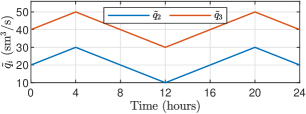
The gas network in Fig. 2 is simulated using the parameter values in Table 1. The pressure at Node 1 is kept constant at $p_{1}=$50\text{\,}\mathrm{bar}\text{/}$$ and the loads at Nodes 2 and 3 are set as in Fig. 3. Furthermore, to investigate the model fidelity in the presence of non-zero inclination angles, the elevation of Node 1 relative to Nodes 2 and 3 is changed to one of the heights $h_{1}\in\{{-1,-0.5,0.5,1}\}$\mathrm{km}\text{/}$$, where $L_{1j}\sin(\theta_{1j})=h_{j}-h_{1}$ with $1j\in\mathcal{E}$. Note that $\theta_{23}=0$.

4.2 Results

Figure 4: Pressures at Node 2.

Figure 5: Pressures at Node 3.

Figure 6: Volumetric flow rates at standard conditions in Pipeline₁₂ and Pipeline₁₃.

Figure 7: Pressure at Node 2 with the respective elevations of Node 1 given on the right.

Figure 8: Pressure at Node 3 with the respective elevations of Node 1 given on the right.

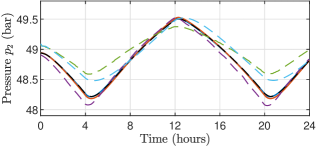
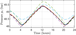
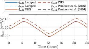
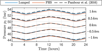
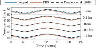
The simulated pressures at Nodes 2 and 3 are shown in Fig. 5 and Fig. 5, respectively, while volumetric flow rates $\tilde{q}_{\mathrm{m},12}$ and $\tilde{q}_{\mathrm{m},13}$ are shown in Fig. 6. Furthermore, the pressures at $p_{2}$ and $p_{3}$ with Node 1 at various elevations are shown Fig. 7 and Fig. 8, respectively. In each case, results are shown for the lumped-parameter model comprising s 1 and 2 and for the PHS model in Theorem 3 where s 1, 2 and 3 are applied.

We note the high level of similarity of both models compared to the results in Pambour et al. (2016). The pressures in both models show deviations of no more than $0.13\text{\,}\mathrm{\char 37\relax}\text{/}$ and the volumetric flow rates of both models exhibit deviations of no more than $1.05\text{\,}\mathrm{\char 37\relax}\text{/}$. Without elevation differences in the network, there is no significant difference in quality between the lumped-parameter and PHS models. However, the effects of s 1, 2 and 3 show more clearly when elevation differences are present. The simulated pressures in Fig. 7 and Fig. 8 show maximal deviations of $0.39\text{\,}\mathrm{\char 37\relax}\text{/}$ for the lumped-parameter model and $0.81\text{\,}\mathrm{\char 37\relax}\text{/}$ for the PHS model. Nevertheless, these errors can be considered sufficiently small for models aimed towards analysis and design.

5 Conclusion

In this paper, we proposed a third-order PHS model for gas pipelines based on the discretized and simplified Euler equations. We showed that this model exhibits the same structure as $\pi$-model transmission lines, can be combined into a PHS model for a gas network, and has passivity properties conducive to passivity-based control. Furthermore, the simulation results demonstrate a model fidelity comparable to that of detailed simulation models. Future work includes exploiting the parallels drawn between the gas and power networks and using the the PHS framework for a conjoined consideration of networked multi-energy systems.

Appendix A Stability for variable mean pressures

We here investigate the stability of the feedback effect as described by 7. Consider therefore the model in Theorem 3 with a non-constant average pressure $p_{\mathrm{M}}$, i.e. 3 does not hold. Rearranging (20) results in

$$p_{\mathrm{M}}=\underbrace{\frac{1}{3}\left(2-\frac{p_{\mathrm{r}}}{p_{\mathrm{l}}+p_{\mathrm{r}}}\right)}_{\textstyle k_{\mathrm{l}}}p_{\mathrm{l}}+\underbrace{\frac{1}{3}\left(2-\frac{p_{\mathrm{l}}}{p_{\mathrm{l}}+p_{\mathrm{r}}}\right)}_{\textstyle k_{\mathrm{r}}}p_{\mathrm{r}},$$ (32)

where $k_{\mathrm{l}},k_{\mathrm{r}}\in(\nicefrac{{1}}{{3}},\nicefrac{{2}}{{3}})$ if $p_{\mathrm{l}}>0$ and $p_{\mathrm{r}}>0$. Substituting (32) into the PHS pipeline dynamics (21a) yields

$$\bm{Q}\!\!\begin{bmatrix}\dot{p}_{\mathrm{l}}\\ \dot{p}_{\mathrm{r}}\\ \dot{\tilde{q}}_{\mathrm{m}}\end{bmatrix}\!=\,\underbrace{\!\!\begin{bmatrix}0&0&-1\\ 0&0&1\\ 1{-}\phi k_{\mathrm{l}}&-1{-}\phi k_{\mathrm{r}}&-\mathcal{R}_{\mathrm{m}}(|\tilde{q}_{\mathrm{m}}|,p_{\mathrm{M}})\end{bmatrix}\!\!}_{\bm{A}}\!\begin{bmatrix}p_{\mathrm{l}}\\ p_{\mathrm{r}}\\ \tilde{q}_{\mathrm{m}}\end{bmatrix}+\begin{bmatrix}\tilde{q}_{\mathrm{l}}\\ \tilde{q}_{\mathrm{r}}\\ 0\end{bmatrix}\!,$$ (33)

where $\phi\coloneqq gL\sin(\theta)/c^{2}$ and with $\bm{Q}$ in (21j). Note that (33) is no longer a PHS, since the symmetric part of the state matrix $\bm{A}$ is no longer positive semi-definite.

Proposition 6

The gas pipeline dynamics with a variable mean pressure described by (33) are Lyapunov stable if

$$L\sin(\theta)<\frac{6c^{2}}{g}.$$ (34)

Since the constant matrix $\bm{Q}$ is positive definite, the Lyapunov stability of (33) can be evaluated by looking at the eigenvalues of the state matrix $\bm{A}$. Specifically, the solution of (33) is guaranteed to be stable if the eigenvalues of $\bm{A}$ are nonpositive everywhere along the state trajectory. The eigenvalues of $\bm{A}$ are

$$\lambda_{1}\!\;{=}\!\;0,\;\;\lambda_{2,3}\!\;{=}-\frac{1}{2}\mathcal{R}_{\mathrm{m}}\pm\frac{1}{2}\sqrt{\mathcal{R}_{\mathrm{m}}^{2}-\!\!\>8\!\!\>-4\phi k_{\mathrm{l}}+4\phi k_{\mathrm{r}}}.$$ (35)

Since $\mathcal{R}_{\mathrm{m}}>0$ (see Theorem 3), positive eigenvalues can only be obtained if the rooted term in (35) is positive. Evaluating where the eigenvalues in (35) are negative when the rooted term is positive thus leads to

$$\frac{1}{2}\sqrt{\mathcal{R}_{\mathrm{m}}^{2}-8-4\phi k_{\mathrm{l}}+4\phi k_{\mathrm{r}}} <\frac{1}{2}\mathcal{R}_{\mathrm{m}}$$ (36)

$$\implies \mathcal{R}_{\mathrm{m}}^{2}-8-4\phi k_{\mathrm{l}}+4\phi k_{\mathrm{r}} <\mathcal{R}_{\mathrm{m}}^{2}$$

$$\iff \phi(k_{\mathrm{r}}-k_{\mathrm{l}}) <2.$$

From (32), we observe that

$$\frac{p_{\mathrm{r}}-p_{\mathrm{l}}}{p_{\mathrm{r}}+p_{\mathrm{l}}}=3(k_{\mathrm{r}}-k_{\mathrm{l}}).$$ (37)

Substituting $\phi=gL\sin(\theta)/c^{2}$ and (37) into (36) gives

$$\frac{p_{\mathrm{r}}-p_{\mathrm{l}}}{p_{\mathrm{r}}+p_{\mathrm{l}}}L\sin(\theta)<\frac{6c^{2}}{g}.$$ (38)

Since (37) is bounded by $[-1,1]$, (34) is obtained as a sufficient condition for (38). ∎ By verifying that (34) holds for a given pipeline, Prop. 6 ensures the stability of the underlying system dynamics. This in turn means that no unstable dynamics are hidden away when applying 3 to obtain the PHS (21). Note that the left-hand side of (34) is the height difference between the two ends of the pipes and that (34) is met in all practical cases.

References

- Alamian et al. (2012) Alamian, R., Behbahani-Nejad, M., and Ghanbarzadeh, A. (2012). A state space model for transient flow simulation in natural gas pipelines. J. Natural Gas Science and Eng., 9, 51–59. 10.1016/j.jngse.2012.05.013.
- Cellier and Kofman (2006) Cellier, F.E. and Kofman, E. (2006). Continuous system simulation. Springer, New York, NY, 1 edition. 10.1007/0-387-30260-3.
- Domschke et al. (2021) Domschke, P., Hiller, B., Lang, J., Mehrmann, V., Morandin, R., and Tischendorf, C. (2021). Gas network modeling: An overview. URL https://opus4.kobv.de/opus4-trr154/frontdoor/index/index/docId/411. Preprint.
- Herrán-González et al. (2009) Herrán-González, A., De La Cruz, J.M., De Andrés-Toro, B., and Risco-Martín, J.L. (2009). Modeling and simulation of a gas distribution pipeline network. Applied Math. Modelling, 33(3), 1584–1600. 10.1016/j.apm.2008.02.012.
- Ke and Ti (2000) Ke, S.L. and Ti, H.C. (2000). Transient analysis of isothermal gas flow in pipeline network. Chemical Eng. J., 76(2), 169–177. 10.1016/S1385-8947(99)00122-9.
- Koch et al. (2015) Koch, T., Hiller, B., Pfetsch, M.E., and Schewe, L. (2015). Evaluating Gas Network Capacities. Society for Industrial and Applied Mathematics, Philadelphia, PA. 10.1137/1.9781611973693.
- Malan et al. (2022) Malan, A.J., Jané-Soneira, P., and Hohmann, S. (2022). Constructive analysis and design of interconnected Krasovskii passive and quadratic dissipative systems. In Proc. 61th IEEE Conf. Decis. Control, 7059–7065. 10.1109/CDC51059.2022.9992956.
- Osiadacz and Chaczykowski (2020) Osiadacz, A.J. and Chaczykowski, M. (2020). Modeling and simulation of gas distribution networks in a multienergy system environment. Proc. IEEE, 108(9), 1580–1595. 10.1109/JPROC.2020.2989114.
- Pambour et al. (2016) Pambour, K.A., Bolado-Lavin, R., and Dijkema, G.P.J. (2016). An integrated transient model for simulating the operation of natural gas transport systems. J. Natural Gas Science and Eng., 28, 672–690. 10.1016/j.jngse.2015.11.036.
- Qadrdan et al. (2019) Qadrdan, M., Fazeli, R., Jenkins, N., Strbac, G., and Sansom, R. (2019). Gas and electricity supply implications of decarbonising heat sector in GB. Energy, 169, 50–60. 10.1016/j.energy.2018.11.066.
- Strehle et al. (2022) Strehle, F., Machado, J.E., Cucuzzella, M., Malan, A.J., Scherpen, J.M., and Hohmann, S. (2022). Port-Hamiltonian modeling of hydraulics in 4th generation district heating networks. In Proc. 61th IEEE Conf. Decis. Control, 1182–1189. 10.1109/CDC51059.2022.9992887.
- Strehle et al. (2020) Strehle, F., Pfeifer, M., Malan, A.J., Krebs, S., and Hohmann, S. (2020). A scalable port-Hamiltonian approach to plug-and-play voltage stabilization in DC microgrids. In 2020 IEEE Conf. Control Technol. and Applications, 787–794. 10.1109/CCTA41146.2020.9206323.
- Taherinejad et al. (2017) Taherinejad, M., Hosseinalipour, S.M., and Madoliat, R. (2017). Dynamic simulation of gas pipeline networks with electrical analogy. J. Brazilian Soc. Mech. Sciences and Eng., 39, 4431–4441. 10.1007/s40430-017-0821-x.
- Weymouth (1912) Weymouth, T.R. (1912). Problems in natural gas engineering. Trans. Am. Soc. Mech. Eng., 34, 185–234.
- Wiid et al. (2020) Wiid, A.J., le Roux, J.D., and Craig, I.K. (2020). Modelling of methane-rich gas pipeline networks for simulation and control. J. of Process Control, 92, 234–245. 10.1016/j.jprocont.2020.06.010.
- Zhou et al. (2017) Zhou, Y., Gu, C., Wu, H., and Song, Y. (2017). An equivalent model of gas networks for dynamic analysis of gas-electricity systems. IEEE Trans. Power Systems, 32(6), 4255–4264. 10.1109/TPWRS.2017.2661762.