Energy landscapes of some matching-problem ensembles

Abstract

The maximum-weight matching problem and the behavior of its energy landscape is numerically investigated. We apply a perturbation method adapted from the analysis of spin glasses. This gives inside into the complexity of the energy landscape of different ensembles. Erdős-Rényi graphs and ring graphs with randomly added edges are considered and two types of distributions for the random edge weighs are used. For maximum-weight matching, fast and scalable algorithms exist, such that we can study large graphs of more than $10^{5}$ nodes. Our results show that the structure of the energy landscape for standard ensembles of matching is simple, comparable to the energy landscape of a ferromagnet. Nonetheless, for some of the here presented ensembles our results allow for the presence of complex energy landscapes in the spirit of Replica-Symmetry Breaking.

Keywords: matching, complexity, perturbation techniques, random graphs, ground states, Replica-Symmetry Breaking, Computer Simulations

1 Introduction

Spin glasses are prototypical complex systems widely studied in statistical physics [1, 2, 3, 4, 5, 6]. The analytical solution of the Sherrington-Kirkpatrick spin glass model [7] led to the notion of Replica-Symmetry Breaking (RSB) [8, 9, 10, 11, 12, 13]. Typical for such a complex RSB phase is a rough energy landscape with many local minimal and metastable states divided by high energy barriers [13]. This leads to non-trivial equilibrium and non-equilibrium behavior.

This concept of complexity is transferable to other problems like neural networks, data analysis or optimization problems [5, 14, 15, 16]. These problems may show behavior like RSB or other types of complexity [17]. It has been observed that, e.g., Satisfiability [18, 19, 20], the traveling salesperson [21, 22, 23], vertex cover [24, 25, 26, 27] and graph coloring [28] can feature complex phases for certain ensembles and model parameters. These models also exhibit rugged energy landscapes with glassy equilibrium and non-equilibrium behavior.

These mentioned problems are members of the class of non-deterministic-polynomial (NP) problems [29]. All known exact algorithms for treating these problems exhibit worst-case running times that grow exponentially with the problem size. This means, one is rather limited in the numerical investigations of the equilibrium behavior of these problems, because only comparable small systems can be studied. This is a pity, because the behavior of these models is very interesting.

On the other hand, in the class of polynomial (P) problems, the worst case run time growths only polynomially. Hence, much larger systems can be studied, leading to numerically more accurate results and better statistics. Unfortunately, problems from P typically feature a simple energy landscape [30, 31, 32, 33, 34, 35], leading to a rather trivial behavior. This seems to indicate that complex behavior and convenient numerical access to the equilibrium behavior do not come together. But it should be noted that most studies so far where performed for model ensembles, where the randomness is introduced in a simple and uncorrelated way. Interestingly, recently a complex behavior was found for ensembles which utilize correlations for the model of directed polymers in random media. For this model a polynomial exact sampling algorithm exists and thus large systems of up to $10^{9}$ lattice sites could be studied and strong indications for replica-symmetry breaking have been observed [36]. Furthermore, for the polynomially tractable problem of increasing subsequences, also called Ulam’s problem, numerical evidence for RSB was found [37]. Finally, it should be noted that also the XOR-SAT problem, which can be solved efficiently by Gaussian elimination [38, 39], exhibits one-step RSB, but this becomes irrelevant in equilibrium in the thermodynamic limit [40].

Thus, by the choice of a suitable ensemble, it seems to be possible to study some systems with non-trivial behavior in a numerically efficient way. In the present work, in the spirit of [36, 37], we study another problem from the class P to seek for indications for complex behavior. In particular, we consider the maximum-weight graph-matching problem. This model was one of the first optimization problems to be studied from the viewpoint of statistical mechanics [41]. Analyses were extended to arbitrary graphs [30], finite-size effects [42] and Euclidean edge weights [43, 44, 45].

The interests of graph-matching problems in physics also comes from the fact that other problems can be solved by a mapping to suitable matching problems. This has been done for, e.g., 2D spin glasses [33], dimer covering [46], negative-weight percolation [47] and controllability of dynamic networks [48, 49].

The remaining of this paper is organized as follows: In section 2, graph matching and random graph ensembles used in this work are introduced. These ensembles are Erdős-Rényi graphs and ring graphs with additional random edges, both with Gaussian distributed or constant edge weights with uniform noise. Section 3 presents the details of the perturbation technique. It it explained how one can investigate whether a complex energy landscape is present by observing the differences between matchings obtained from the original and slightly perturbed graphs, respectively. We also address the question whether the perturbation approach can be used to sample matching statistically correctly. The results of the analyses are given in section 4, where we start with the results obtained from the perturbation technique. We summarize and draw final conclusions in section 5.

2 Model

2.1 Matching

An undirected graph $G=\left(V,E\right)$ is given by a set of nodes $i\in V$ and a set of edges $e\in E\subseteq V^{(2)}$, where $n=\left|V\right|$ and $m=\left|E\right|$. Two nodes $i$ and $j$ are called adjacent if $e=\left\{i,\,j\right\}$ is a member of $E$. This edge $e$ called incident to $i$ and $j$. A matching $M$ is a subset of $E$ in which no two edges are incident to the same node. For each edge in $M$, its adjacent nodes are called matched. Nodes which are not matched are called free. A maximum cardinality matching is a matching with maximizes the number of matched nodes $\left|M\right|$. On a graph $G$ with edge weights $w(e)$, the weight of the matching is $W=\sum_{e\in M}w(e)$. A maximum-weight matching is a matching $M$ that maximizes the weight $W$ over all possible matchings on $G$. In section 3 we state the algorithm we have used to obtain the maximum-weight matching of a given graph.

2.2 Random graphs

We consider two types of random graph ensembles. Details on the chosen values of the model parameters are given in section 4. The first ensemble consists of Erdős-Rényi random graphs [50]. To generate such graphs, one starts with on empty graph of $n$ nodes $V=\{1,2,\cdots,n\}$. Then, for each possible pair of distinct nodes, an edge is created independently with probability $p=c/n$, where $c$ is the connectivity. The resulting degree distribution is Poissonian.

The second ensemble consist of ring graphs with additional random edges. First, a regular ring graph with mean degree of two is created. This means, the edge $E$ set initially contains the edges $\{i,i+1\}$ for $i=1,\ldots,n-1$ plus the edge $\{n,0\}$. Next, two nodes $i,j$ are chosen randomly with uniform probability and the edge $\left\{i,j\right\}$ is created if $i\neq j$ and $\left\{i,j\right\}$ does not yet exist in $E$. This process is repeated until $m^{+}$ edges are added to the graph this way. The number of edges in $G$ is then given by $m=n+m^{+}$. Below we will consider the cases $m^{+}=$ const, $m^{+}\in O(\log n)$ and $m^{+}\in O(n)$.

Two types of edge weights $w(e)$ are investigated. First, we consider $w(e)\sim\mathcal{N}(1,0.01)$, i.e., Gaussian distributed random weights with a mean of 1 and a variance of $0.01$. Second, we study constant weights with additional uniform noise, $w(e)=1+\varepsilon$. To choose the strength of the additional noise $\varepsilon$, we mention that with $w(e)=1$ for all edges, a maximum-weight matching is equivalent to a maximum cardinality matching, since $W=\left|M\right|$ holds. The purpose of the additive noise $\varepsilon$ is to make the optimal solution unique. But beside that, it should not influence the size of the optimum matching even for large values of $n$. To ensures that, $\varepsilon$ is drawn from a uniform distribution where the values scale with $n^{-\frac{1}{2}}$, i.e., $\varepsilon\sim U(-0.01\,n^{-\frac{1}{2}},\ 0.01\,n^{-\frac{1}{2}})$.

3 Methods

To find a maximum weight matching we use Edmond’s Blossom Shrinking algorithm [51], implemented in the LEMON-library [52]. The algorithm has a worst-case running time $O(n^{2}m)$, i.e., polynomial, such that correspondingly large graphs can be treated.

3.1 Perturbation technique

When studying the complexity of energy landscapes, a common technique is to apply weak perturbations on the system. To our knowledge, this technique was first used to study spin glasses (see, e.g., [53]). Since then, it was adapted for, e.g., random-field Ising models [54, 55] and the traveling salesperson problem [23].

The basic idea is to first calculate a ground state and the perturb the system slightly such that by a recomputation a new ground state is obtained, which is an excited state with respect to the original system. For the matching problem, we use edge flips as a perturbation technique. First, a maximum-weight matching $M_{0}$ with total weight $W_{0}$ is calculated. Then, one randomly chosen edge $e$ will be “flipped”. If $e$ is in $M_{0}$, it is not allowed to be in a matching $M_{1}$ of the perturbed graph. On the other hand, if $e$ is not in $M_{0}$, it is enforced to be in $M_{1}$. In practice, this can be achieved by setting the weight of $e$ to a very small value, e.g., $-2W_{0}$, or a very large value, e.g., $2W_{0}$, respectively. After $M_{1}$ is found, the weight of the edge will be reset to its original value such that the weight $W_{1}$ of $M_{1}$ is calculated with the original weights. In the following, $M_{0}$ will always denote an optimal matching with respect to the original edge weights, while $M_{i}$ with $i>0$ denote independent matchings resulting from perturbations by a single edge flip with respect to $M_{0}$. $W_{0}$ and $W_{i}$ denote the corresponding weights of the matchings.

A perturbation is weak if the relative difference of $W_{0}$ and $W_{1}$ behaves as

$$\frac{W_{0}-W_{1}}{W_{0}}=\Or\left(\frac{1}{n}\right).$$ (1)

If (1) holds, $M_{1}$ is quasi optimal. Note that this means that when considering the system in the canonical ensemble, i.e., according to the Boltzmann distribution, the matchings $M_{0}$ and $M_{1}$ will contribute with the same weight in the thermodynamic limit.

To compare two matchings $M_{i}$ and $M_{j}$, we apply a similarity measure, also called overlap. Since matchings are sets, it is convenient to use the Jaccard index [56], given by

$$q_{ij}=\frac{\left|M_{i}\cap M_{j}\right|}{\left|M_{i}\cup M_{j}\right|}.$$ (2)

The distance between two matchings is defined as $d_{ij}=1-q_{ij}$ [57]. Overlap and distance between optimal matching $M_{0}$ and matching $M_{i}$ obtained from a perturbation are denoted as $q_{0}$ and $d_{0}$, respectively, where the second index $i$ is omitted.

A necessary condition for a complex energy landscape is that there exist quasi optimal matchings with $d_{0}>0$ in the thermodynamic limit of infinite large graphs [58]. Hence, we measured $\left\langle(W_{0}-W_{i})/W_{0}\right\rangle$ and $\left\langle d_{0}\right\rangle$ for different values of $n$, averaged over random graph realizations. If the matchings for the perturbed graphs are quasi optimal and $\left\langle d_{0}\right\rangle$ converges towards zero for increasing values of $n$, a simple energy landscape can be assumed. But if $\left\langle d_{0}\right\rangle$ remains finite, a complex energy landscape can not be excluded.

3.2 Sampling bias test

To further investigate whether the matching problem on a given graph ensemble indeed exhibits a complex energy landscape, it would be desirable to efficiently sample matchings. For correct statistics, matchings with equal total weight $W$ should be sampled with equal probability. Hence, a sampling approach needs to know the number of distinct matchings for the full problem and for encountered subproblems. Unfortunately, the matching problem is in the class of #P-complete problems [59, 60]. This means, with all known algorithms, it requires to enumerate all matchings, which are typically exponentially many. Hence, such an approach is computationally demanding.

We can, in principle, use matchings obtained by the perturbation method as samples. Unfortunately, edge flips create an unknown bias to the sampling because various configurations are prohibited, which depends on the flipped edge. It could nonetheless be the case that bias errors average out, especially for large graphs. To assess this, we have performed the following investigation.

For a given graph, here we study Erdős-Rényi graphs, a set of edge weights of constant weights with noise $w=1+\varepsilon$ is drawn, see section 2.2. Then, an optimal matching according to this set of weights is calculated. Next, multiple times a perturbed graph is obtained, using random edge flips, and again matchings are calculated. This process is then repeated for multiple realizations of the initial noise.

The obtained matchings are collected in a sample histogram. Here, we include only matchings with the same cardinality as the optimal matching. The resulting histogram is then used to compare the relative frequencies $Q(M)$ to the case where all matchings would have been drawn with equal probability. That is $P(M)=1/n_{\mathrm{M}}$, where $n_{\mathrm{M}}$ is the number distinct matchings. As the number of matchings grows exponentially with the number of edges, this procedure is only appropriate for small graphs.

To compare $P$ and $Q$ quantitatively, two distance measures are used. The first one is the Kullback-Leibler divergence $D_{\mathrm{KL}}$ defined as

$$D_{\mathrm{KL}}(P,Q)=\sum_{i=1}^{n_{\mathrm{M}}}P(M_{i})\ln\left(\frac{P(M_{i})}{Q(M_{i})}\right).$$ (3)

The second measure is the mean relative error $\mathrm{MRE}$ given by

$$\mathrm{MRE}(P,Q) =\sum_{i=1}^{n_{\mathrm{M}}}P(M_{i})\frac{\sqrt{\left(P(M_{i})-Q(M_{i})\right)^{2}}}{P(M_{i})}$$ (4)

$$=\sum_{i=1}^{n_{\mathrm{M}}}\sqrt{\left(P(M_{i})-Q(M_{i})\right)^{2}},$$ (5)

which is the averaged relative error per matching.

If $P$ and $Q$ become more equal for larger graphs, the values of $D_{\mathrm{KL}}$ and $\mathrm{MRE}$ will become smaller. In particular, if the sampling approaches the uniform one, the distance measures should converge to zero. If this was the case, the overlap distributions $P(q)$ could be investigated in a meaningful way. In case the distribution of overlaps remains broad in the limit of large graphs, this would indicate that a complex behavior is significant in equilibrium. On the other hand, if the values of $D_{\mathrm{KL}}$ and $\mathrm{MRE}$ increase with larger graphs, the sampling bias errors can not be neglected. In this case, a limiting nonzero value of the distance $d_{0}$ would only indicate that significantly different matchings exists, but one would not know by using the present approach whether their weights are strong enough to influence the equilibrium behavior.

4 Results

The following results are obtained by performing simulations [61] for the two graph ensembles, various values of parameters and graph sizes in the range of $n=7$ to $131\,072$. If not otherwise specified, all results are averaged over 100 different random graph realizations and 100 different edge-flip perturbations and resulting matchings for each graph realization. Partially, the GNU Parallel tool was used to distribute the simulations over several CPUs [62]. All data fits were performed as recommended in Ref. [63].

4.1 Perturbation

We first verify that the matchings of the perturbed graphs are quasi optimal. Our results show that for both types of random graphs, Erdős-Rényi and ring graphs, as well as for both types of edge weights, the matchings for the perturbed graphs are quasi optimal as (1) holds. In figure 1, results are shown for Erdős-Rényi graphs with connectivities $c\in\left\{0.5,\,1,\,2,\,4\right\}$. Included are results from fits using

$$\left\langle\left(W_{0}-W_{i}\right)/W_{0}\right\rangle=\alpha\,\frac{1}{n}.$$ (6)

In the other studied cases the results look similar, hence they are not shown here. Note that for ring graphs, the data deviates from the fit for small sizes $n\leq 2^{8}$. Since (1) is required to hold only asymptotically, the condition for quasi optimality is fulfilled for this case as well.

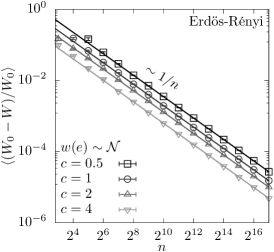
Figure 1: Verification that the matchings on perturbed graphs are quasi optimal, as $\left\langle(W_{0}-W)/W_{0}\right\rangle$ as a function of $n$ behaves as $\Or(1/n)$. Shown here are results for Erdős-Rényi graphs with Gaussian distributed random weights and connectivities $c\in\left\{0.5,\,1,\,2,\,4\right\}$. The straight lines represent fits in the form of (6).

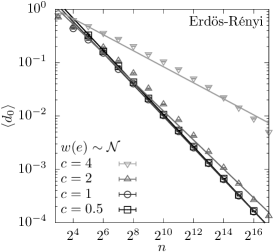
Figure 2: Averaged distance $\left\langle d_{0}\right\rangle$ between matchings on perturbed graphs and optimal matchings as a function of $n$ for Erdős-Rényi graphs with Gaussian distributed random weights and connectivities $c\in\left\{0.5,\,1,\,2,\,4\right\}$. The straight lines represent power low fits in the form of (7).

We next look at the behavior of $d_{0}$ and start with the case of Gaussian distributed weights. The results for Erdős-Rényi graphs are shown in figure 2. One observes that the distance $\left\langle d_{0}\right\rangle$ approaches zero for increasing $n$. To confirm this behavior systematically, a power law fit with offset $d_{\infty}$ is used,

$$\left\langle d_{0}\right\rangle(n)=d_{\infty}+\beta_{1}\,n^{\beta_{2}}\,,$$ (7)

resulting in good fits. The resulting fit parameters for all studied cases are reported in table 1.

Table 1: Values of the fit parameters for the fits in the form of $(\ref{eq:fit_d0})$ to determine $d_{\infty}$. Fixed values are marked with *. Results are given for various values of parameters (first column) and edge weights (second column) for Erdős-Rényi graphs and ring graphs with even or odd number of edges. A value of $d_{\infty}=0$ corresponds to a simple energy landscape. But for $d_{\infty}>0$, a complex behavior can not be excluded. Values for $\beta_{1}$ and $\beta_{2}$ are given for completeness.

Erdős-Rényi graphs
$c$	$w$	$d_{\infty}$	$\beta_{1}$	$\beta_{2}$
$0.5$	$\sim\mathcal{N}$	0*	$10.7(1)$	$0.997(1)$
$1$	$\sim\mathcal{N}$	0*	$8.8(1)$	$0.982(1)$
$2$	$\sim\mathcal{N}$	0*	$6.27(7)$	$0.898(1)$
$4$	$\sim\mathcal{N}$	0*	$2.18(2)$	$0.446(1)$
$0.5$	$1+\varepsilon$	0*	$10.8(2)$	$0.998(2)$
$1$	$1+\varepsilon$	0*	$8.9(1)$	$0.983(1)$
$2$	$1+\varepsilon$	0*	$6.36(7)$	$0.901(1)$
$4$	$1+\varepsilon$	0*	$2.65(2)$	$0.499(1)$
ring graphs, $n$ even
$m^{+}(n)$	$w$	$d_{\infty}$	$\beta_{1}$	$\beta_{2}$
$0$	$\sim\mathcal{N}$	0*	$83(3)$	$0.989(3)$
$1$	$\sim\mathcal{N}$	0*	$81(3)$	$0.986(3)$
$10$	$\sim\mathcal{N}$	0*	$80(2)$	$0.985(3)$
$0$	$1+\varepsilon$	1*	0*	0*
$1$	$1+\varepsilon$	$0.947(2)$	0*	0*
$10$	$1+\varepsilon$	$0.583(3)$	$2.5(5)$	$1.16(9)$
$2\,\ln(n)$	$1+\varepsilon$	$0.345(5)$	$1.00(3)$	$0.35(1)$
$4\,\ln(n)$	$1+\varepsilon$	$0.255(3)$	$1.31(3)$	$0.42(1)$
ring graphs, $n$ odd
$m^{+}(n)$	$w$	$d_{\infty}$	$\beta_{1}$	$\beta_{2}$
$0$	$\sim\mathcal{N}$	0*	$81(3)$	$0.987(3)$
$1$	$\sim\mathcal{N}$	0*	$79(3)$	$0.984(3)$
$10$	$\sim\mathcal{N}$	0*	$84(2)$	$0.991(3)$
$0$	$1+\varepsilon$	$0.544(3)$	$1.5(5)$	$1.1(2)$
$1$	$1+\varepsilon$	$0.523(3)$	$2.0(5)$	$1.1(1)$
$10$	$1+\varepsilon$	$0.397(3)$	$2.2(2)$	$0.92(4)$
$2\,\ln(n)$	$1+\varepsilon$	$0.295(3)$	$1.42(6)$	$0.56(2)$
$4\,\ln(n)$	$1+\varepsilon$	$0.222(3)$	$1.50(4)$	$0.51(1)$

For Gaussian distributed weights, the value of $d_{\infty}$ is set to a fixed value of zero in all cases to obtain reasonable results. Fits with a freely estimated $d_{\infty}$ result in negative values for this parameter, i.e., nonphysical results. The observed behavior shows that the matchings for the perturbed graphs share most of their edges with the matching for the original graphs, increasingly with growing system size. This can be explained by the application of a non-uniform weight distribution. To maximize $W_{0}$, the matching algorithm focuses on few edges with large weights. Now for a matching with perturbed weights, if one edge is flipped, a large total weight is still achieved by using most of the same edges with large weights as in $M_{0}$. Consequently, only a few edges change compared to $M_{0}$ to compensate the edge flip. This results in a small difference between optimal matching and matching of the perturbed graph that vanishes in the limit of infinity large graphs.

Overall, the results for Gaussian weights indicate a simple structure of the energy landscape. The results for ring graphs are similar and therefore not shown here. As constant values of $m^{+}$ result in $d_{\infty}=0$, we omitted to investigate values of $m^{+}\in O(\log n)$ or $m^{+}\in O(n)$ for Gaussian distributed weights.

We next look at constant edge weights with additional noise. Since here all edge weights are more similar to each other, the existence of very different matchings with very similar weight, i.e., a more complex energy landscape, can be anticipated. For Erdős-Rényi graphs the results for $\left\langle d_{0}\right\rangle$ are similar to the above discussed case with Gaussian distributed weights, and therefore no shown here. Again, fixed values of $d_{\infty}=0$ are needed to obtain physically meaningful results for the fits according to (7). Thus, also for this case no sign of a complex energy landscape can be found.

The argumentation for Gaussian weights no longer holds here since each edge is almost equally important for the total weight. But here, the topological constrains of Erdős-Rényi graphs explain the behavior: Since loops are of order $\log(n)$ for Erdős-Rényi graphs, local changes of the matching do not spread far, resulting only in small overall differences between the optimum matching for the original and the perturbed graph. Hence, the difference $\left\langle d_{0}\right\rangle$ vanishes for $n\to\infty$.

On the other hand, for ring graphs the behavior is different, as it can also be seen in figure 3. Here, a value of $d_{\infty}>0$ was needed for a good fit in all studied cases.

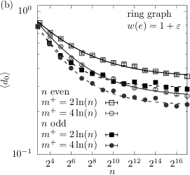
Figure 3: Averaged distance $\left\langle d_{0}\right\rangle$ between matchings on perturbed graphs and optimal matchings as a function of $n$ for ring graphs. (a) shows results for constant edge weights with additional noise and values of $m^{+}\in\left\{0,\,1,\,10\right\}$ and (b) shows results for $m^{+}=l^{+}\ln(n)$ with $l^{+}\in\left\{2,\,4\right\}$. Blank symbols indicate even number of nodes $n$, while filled symbols are used for odd values of $n$. The straight or dashed lines represent power low fits with offset $d_{\infty}$ in the form of (7), respectively.

To understand this behavior, consider ring graphs with an even number $n$ of nodes and no random edges, i.e., $m^{+}=0$. Since matchings along paths appear as alternations of matched and free edges, the simple ring graph structure enforces that all matchings $M_{i}$ with $i>0$ are given by $E\setminus M_{0}$, i.e., all matched edges are replaced by free ones, and vice-versa. Hence, trivially $d_{0}=1$ holds.

If $n$ is odd, one node remains free and there are $n$ maximum cardinality matchings. $M_{0}$ is given by the maximum cardinality matchings with the largest total weight. Using $E\setminus M_{0}$ for a perturbed graph would results in lower cardinality of the matchings and hence lower total weight. However, $n-1$ other matchings remain to compensate for the edge flip, each of which leaves another node free. Thus, one average about half of the edges change in the optimum matching when the graph is perturbed. This can be compared to a simple spin system: for a ferromagnet when anti-periodic boundary conditions are introduced, two domain walls will be created, one where the new boundary conditions are located, the other one anywhere in the system. This also results in many different configurations, but the system still actually does not behave in a complex way. In conclusion, that $d_{\infty}$ stays finite for $m^{+}=0$ for the simple ring graph is not resulting from a complex energy landscape, but rather from the simple structure of the graphs.

When adding random edges, the situation becomes more interesting. The perturbation leads for the cases of $m^{+}=$ const and $m^{+}\in O(\ln n)$ to various matchings and more complex overlaps between the matchings become possible. The finite value of $d_{\infty}$ can no longer be explained by the graph structure alone. Hence, we observe quasi optimal solutions that differ from the optimal solution by an extensive number of edges. This is a necessary condition for complexity [58]. Thus a complex energy landscape may exist for this ensemble.

We also performed simulations with ring graphs where the number of random edges $m^{+}$ grows linearly with $n$. Here, the ring graphs become increasingly equal to Erdős-Rényi graphs for large values of $n$ and the ring structure becomes less important. Hence, similar findings as for Erdős-Rényi graphs were obtained, i.e., we observed $\langle d_{0}\rangle\to 0$ for $n\to\infty$. Therefore, we do not report further results for this case.

4.2 Sampling

Our previous results show that there exists ensembles for the matching problem, where optimum matchings exists, which differ by $O(n)$ variables but almost have the same energy, i.e., are quasi optimal. This is a necessary condition for the existence of a complex energy landscape. As mentioned above, it would be desirable to sample these matchings and compare them to each other, to understand the energy landscape better, in particular in the thermodynamic limit. For this purpose sampling with equal probability, i.e., in an unbiased way, is needed.

For the sampling bias test, Erdős-Rényi graphs with $1+\epsilon$ weights, $c=2$ and $n$ between 4 and 32 are used. Note that fully enumerating all solutions and sampling with good statistics is only feasible for such small sizes. For each graph $1000$ different sets of edge weights are used and $1000$ matchings for the perturbed graphs are calculated for each of these weight sets, resulting in $10^{6}$ matchings for each graph.

The frequencies $Q(M_{i})$ of occurrences of these matchings are measured and compared to the required uniform distribution as described in section 3.2. The obtained values of $D_{\mathrm{KL}}$ and $\mathrm{MSE}$ are averaged over 100 different random graph realizations. This averaging is denoted by $\left\langle.\right\rangle_{\mathrm{G}}$. Results are shown in figure 4. Here it can be seen that both $\left\langle D_{\mathrm{KL}}\right\rangle_{\mathrm{G}}$ and $\left\langle\mathrm{MSE}\right\rangle_{\mathrm{G}}$ increase for increasing values of $n$. Hence, the sampling bias does not average out. It can also be seen that the error bars increase with larger values of $n$. This is the case, because the number of possible matchings grow with the number $n$ of nodes resulting in an increasing variance.

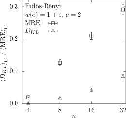
Figure 4: Result of the sampling bias test. Averaged Kullback-Leibler divergence $\left\langle D_{\mathrm{KL}}\right\rangle_{\mathrm{G}}$ and mean relative error $\left\langle\mathrm{MRE}\right\rangle_{\mathrm{G}}$ both systematically increase with larger values of $n$. The results are obtained from Erdős-Rényi graphs with a connectivity of $c=2$ and constant edge weights with additional noise.

This result shows that the sampling error does not averages out. Hence, it is not meaningful to investigate sampled overlap distributions $P(q)$ with samples directly drawn from the perturbation process.

5 Conclusion

We have studied the behavior of the energy landscape of matchings by using “edge flips” to perturb the optimal solution of the original graphs. Our analyses have shown that for suitable ensembles there exist quasi optimal states with differ from the ground state by an extensive number of edges. Hence, a complex energy landscape can not be excluded here. These ensembles include ring graphs with a constant or logarithmic growing number of additional edges and constant edge weights with uniform noise. In these cases, the extrapolated relative distance $d_{\infty}$ between the matchings stays finite. For the other observed ensembles, ring graphs with linear growing number of extra edges and for Erdős-Rényi graphs, the results show no evidence for a complex energy landscape.

It was shown that samples taken directly from the perturbation method are biased. This hindered further more detailed investigations, like obtaining the distribution of overlaps between many optimum matchings. Hence, it is unknown if the quasi optimal states are relevant in the thermodynamic limit. If this was not the case, the behavior of the energy landscape observed here resembles “weakly broken replica symmetry” [64]. It should be noted that, in general, approaches based on perturbing given optimum solutions are only able to show whether there exist other solutions which differ by $O(n)$ variables, but not whether they are relevant in the thermodynamic limit. Still, if these very different other quasi-optimal solutions do not exist, it is clear that the energy landscape is simple.

To set up further studies, it should be noted that for ring graphs with a constant or logarithmically growing number $m^{+}(n)$ of additional edges, a finite value of $d_{\infty}>0$ was observed. But if $m^{+}(n)$ grows linearly with $n$, we found $d_{\infty}=0$. Consequently, there exist a transition between choices for $m^{+}(n)$ where $d_{\infty}$ remains finite and where it vanishes. To analyses this further, the number of extra edges could be modeled by a power law $m^{+}\in O(n^{\lambda})$. Then, it can be evaluated if a critical value $\lambda_{c}$ for the exponent exists, where a sudden transition between $d_{\infty}>0$ and $d_{\infty}=0$ takes place.

Also, it would be interesting to find a method to efficiently draw unbiased samples. One could use sampling methods which are numerically more demanding, like Monte Carlo Markov-chain simulations [65] or exhaustive enumerations. With present algorithms this would restrict the accessible system sizes considerable. On the other hand, it could be possible to correct the sampling bias afterwards using the ballistic-search approach [66], which has been applied successfully to correct the sampling bias observed for evolutionary algorithms when applied to spin glasses [67]. This is algorithmically quite demanding, but certainly feasible in future projects. By applying such approaches, the sampled overlap distributions $P(q)$ can then be investigated to get more inside into the energy landscape of the ensembles proposed here. In this way, it would also possible to check whether the quasi-optimal very different solutions are relevant in the thermodynamic limit.

Beside matching and directed polymers, other P problems may also show indications of a complex energy landscape for suitable ensembles. The methods described in this or other works [38, 39, 36, 37] can be adjusted to these problems to studied them in a similar fashion.

References

- [1] Binder K and Young A P 1986 Rev. Mod. Phys. 58(4) 801–976 URL https://link.aps.org/doi/10.1103/RevModPhys.58.801
- [2] Mézard M, Parisi G and Virasoro M A 1987 Spin glass theory and beyond: An Introduction to the Replica Method and Its Applications vol 9 (World Scientific, Singapore)
- [3] Fischer K H and Hertz J A 1993 Spin glasses 1 (Cambridge university press)
- [4] Young A P 1998 Spin glasses and random fields vol 12 (World Scientific, Singapore)
- [5] Nishimori H 2001 Statistical physics of spin glasses and information processing: an introduction 111 (Oxford University Press, Oxford)
- [6] Kawashima N and Rieger H 2013 Frustrated Spin Systems 509–614
- [7] Sherrington D and Kirkpatrick S 1975 Phys. Rev. Lett. 35(26) 1792–1796 URL https://link.aps.org/doi/10.1103/PhysRevLett.35.1792
- [8] Parisi G 1979 Physics Letters A 73 203–205 ISSN 0375-9601 URL https://www.sciencedirect.com/science/article/pii/0375960179907084
- [9] Parisi G 1979 Phys. Rev. Lett. 43(23) 1754–1756 URL https://link.aps.org/doi/10.1103/PhysRevLett.43.1754
- [10] Parisi G 1980 Journal of Physics A: Mathematical and General 13 1887–1895 URL https://doi.org/10.1088/0305-4470/13/5/047
- [11] Parisi G 1980 Journal of Physics A: Mathematical and General 13 L115–L121 URL https://doi.org/10.1088/0305-4470/13/4/009
- [12] Parisi G 1980 Journal of Physics A: Mathematical and General 13 1101–1112 URL https://doi.org/10.1088/0305-4470/13/3/042
- [13] Parisi G 1983 Phys. Rev. Lett. 50(24) 1946–1948 URL https://link.aps.org/doi/10.1103/PhysRevLett.50.1946
- [14] Hartmann A K and Weigt M 2005 Phase transitions in combinatorial optimization problems : basics, algorithms and statistical mechanics (Weinheim: Wiley-VCH) ISBN 3527404732
- [15] Mezard M and Montanari A 2009 Information, physics, and computation (Oxford: Oxford University Press)
- [16] Moore C and Mertens S 2016 The nature of computation reprinted 2016 (with corrections) ed (Oxford: Oxford University Press) ISBN 9780199233212
- [17] Franchini S 2022 arXiv URL https://arxiv.org/abs/1610.03941v12
- [18] Kirkpatrick S and Selman B 1994 Science 264 1297–1301 URL https://www.science.org/doi/abs/10.1126/science.264.5163.1297
- [19] Hayes B 1997 American Scientist 85 108–112 ISSN 00030996 URL http://www.jstor.org/stable/27856726
- [20] Cocco S and Monasson R 2001 Phys. Rev. Lett. 86(8) 1654–1657 URL https://link.aps.org/doi/10.1103/PhysRevLett.86.1654
- [21] Gent I P and Walsh T 1996 Artificial Intelligence 88 349–358 ISSN 0004-3702 URL https://www.sciencedirect.com/science/article/pii/S0004370296000306
- [22] Schawe H and Hartmann A K 2016 EPL 113 30004 URL https://doi.org/10.1209/0295-5075/113/30004
- [23] Schawe H, Jha J K and Hartmann A K 2019 Phys. Rev. E 100(3) 032135 URL https://link.aps.org/doi/10.1103/PhysRevE.100.032135
- [24] Weigt M and Hartmann A K 2000 Phys. Rev. Lett. 84(26) 6118–6121 URL https://link.aps.org/doi/10.1103/PhysRevLett.84.6118
- [25] Hartmann A K and Weigt M 2001 Theoretical Computer Science 265 199–225 ISSN 0304-3975 phase Transitions in Combinatorial Problems URL https://www.sciencedirect.com/science/article/pii/S0304397501001633
- [26] Weigt M and Hartmann A K 2001 Phys. Rev. Lett. 86(8) 1658–1661 URL https://link.aps.org/doi/10.1103/PhysRevLett.86.1658
- [27] Weigt M and Hartmann A K 2001 Phys. Rev. E 63(5) 056127 URL https://link.aps.org/doi/10.1103/PhysRevE.63.056127
- [28] Mulet R, Pagnani A, Weigt M and Zecchina R 2002 Phys. Rev. Lett. 89(26) 268701 URL https://link.aps.org/doi/10.1103/PhysRevLett.89.268701
- [29] Garey M R and Johnson D S 1979 Computers and intractability vol 174 (San Francisco: W.H. Freeman)
- [30] Mézard M and Parisi G 1987 Journal de Physique 48 1451–1459
- [31] Middleton A A and Fisher D S 2002 Phys. Rev. B 65(13) 134411 URL https://link.aps.org/doi/10.1103/PhysRevB.65.134411
- [32] Hartmann A K and Moore M A 2003 Phys. Rev. Lett. 90(12) 127201 URL https://link.aps.org/doi/10.1103/PhysRevLett.90.127201
- [33] Hartmann A K and Moore M A 2004 Phys. Rev. B 69(10) 104409 URL https://link.aps.org/doi/10.1103/PhysRevB.69.104409
- [34] Ahrens B and Hartmann A K 2011 Phys. Rev. B 84(14) 144202 URL https://link.aps.org/doi/10.1103/PhysRevB.84.144202
- [35] Münster L, Norrenbrock C, Hartmann A K and Young A P 2021 Phys. Rev. E 103(4) 042117 URL https://link.aps.org/doi/10.1103/PhysRevE.103.042117
- [36] Hartmann A K 2022 Europhysics Letters 137 41002 URL https://dx.doi.org/10.1209/0295-5075/ac5226
- [37] Krabbe P, Schawe H and Hartmann A K 2023 Phys. Rev. B 107(6) 064208 URL https://link.aps.org/doi/10.1103/PhysRevB.107.064208
- [38] Ricci-Tersenghi F, Weigt M and Zecchina R 2001 Phys. Rev. E 63(2) 026702
- [39] Mézard M, Ricci-Tersenghi F and Zecchina R 2003 J. Stat. Phys. 111 505
- [40] Ricci-Tersenghi F 2010 Science 330 1639–1640
- [41] Mézard M and Parisi G 1985 Journal de Physique Lettres 46 771–778
- [42] Parisi G and Ratiéville M 2002 The European Physical Journal B-Condensed Matter and Complex Systems 29 457–468
- [43] Mézard M and Parisi G 1988 Journal de Physique 49 2019–2025
- [44] Houdayer J, De Monvel J B and Martin O 1998 The European Physical Journal B-Condensed Matter and Complex Systems 6 383–393
- [45] Caracciolo S, Lucibello C, Parisi G and Sicuro G 2014 Physical Review E 90 012118
- [46] Kenyon R 2009 Lectures on dimers arXiv:0910.3129
- [47] Melchert O, Norrenbrock C and Hartmann A 2014 Physics Procedia 57 58 – 67 ISSN 1875-3892 proceedings of the 27th Workshop on Computer Simulation Studies in Condensed Matter Physics (CSP2014) URL http://www.sciencedirect.com/science/article/pii/S1875389214002776
- [48] Liu Y Y, Slotine J J and Barabási A L 2011 Nature 473 167
- [49] Menichetti G, Dall’Asta L and Bianconi G 2014 Phys. Rev. Lett. 113(7) 078701 URL https://link.aps.org/doi/10.1103/PhysRevLett.113.078701
- [50] Erdős P and Rényi A 1959 Publicationes Mathematicae 6 290–297
- [51] Cook W J, Cunningham W H, Pulleyblank W R and Schrijver A 1998 Combinatorial Optimization (New York, NY, USA: John Wiley & Sons, Inc.) ISBN 0-471-55894-X
- [52] Egerváry Research Group on Combinatorial Optimization LEMON stands for Library for Efficient Modeling and Optimization in Networks. It is a Open Sorce C++ Library. http://lemon.cs.elte.hu/pub/doc/1.2.3/index.html
- [53] Palassini M and Young A P 2000 Phys. Rev. Lett. 85(14) 3017–3020 URL https://link.aps.org/doi/10.1103/PhysRevLett.85.3017
- [54] Zumsande M, Alava M J and Hartmann A K 2008 Journal of Statistical Mechanics: Theory and Experiment 2008 P02012
- [55] Zumsande M and Hartmann A K 2009 The European Physical Journal B 72 619–627
- [56] Jaccard P 1912 New Phytologist 11 37–50
- [57] Levandowsky M and Winter D 1971 Nature 234 34–35
- [58] Mézard M and Parisi G 1986 Journal de Physique 47 1285–1296
- [59] In [68] is was shown that perfect matchings on bipartite graphs are #P-complete. Each graph has a bipartite subgraph and this subgraph has at least as many matchings as perfect matchings. Hence, it follows that also matching is #P-complete.
- [60] Vazirani V V 2002 Approximation Algorithms (Berlin Heidelberg: Springer) chapter 28
- [61] Hartmann A K 2015 Big Practical Guide to Computer Simulations (Singapore: World Scientific)
- [62] Tange O 2020 Gnu parallel 20210322 (’2002-01-06’) GNU Parallel is a general parallelizer to run multiple serial command line programs in parallel without changing them. URL https://doi.org/10.5281/zenodo.4628277
- [63] Young P 2014 Everything you wanted to know about Data Analysis and Fitting but were afraid to ask arXiv:1210.3781v3
- [64] Parisi G 1990 J. Phys. France 51 1595 – 1606
- [65] Newman M E J and Barkema G T 1999 Monte Carlo Methods in Statistical Physics (Oxford: Clarendon Press)
- [66] Hartmann A K 2000 J. Phys. A 33 657
- [67] Hartmann A K and Ricci-Tersenghi F 2002 Phys. Rev. B 66 224419
- [68] Valiant L 1979 Theoretical Computer Science 8 189–201 ISSN 0304-3975 URL https://www.sciencedirect.com/science/article/pii/0304397579900446