The synthetic instrument: From sparse association to sparse causation

Abstract

In many observational studies, researchers are often interested in studying the effects of multiple exposures on a single outcome. Standard approaches for high-dimensional data such as the lasso assume the associations between the exposures and the outcome are sparse. These methods, however, do not estimate the causal effects in the presence of unmeasured confounding. In this paper, we consider an alternative approach that assumes the causal effects in view are sparse. We show that with sparse causation, the causal effects are identifiable even with unmeasured confounding. At the core of our proposal is a novel device, called the synthetic instrument, that in contrast to standard instrumental variables, can be constructed using the observed exposures directly. We show that under linear structural equation models, the problem of causal effect estimation can be formulated as an $\ell_{0}$-penalization problem, and hence can be solved efficiently using off-the-shelf software. Simulations show that our approach outperforms state-of-art methods in both low-dimensional and high-dimensional settings. We further illustrate our method using a mouse obesity dataset.

Keywords: Causal inference; Multivariate analysis; Unmeasured confounding.

1 Introduction

Sparsity is a common assumption in modern statistical learning literature, as it allows one to perform variable selection in an underlying model, and enhances interpretability in the parameter estimates. For example, the lasso method (Tibshirani, 1996) assumes that the underlying associations between a single outcome and potentially high-dimensional predictors are sparse. In other words, only a small number of predictors have non-zero associations with the outcome. Hastie et al. (2009) summarize the philosophy behind these methods as the “bet on sparsity” principle: Use a procedure that does well in sparse problems since no procedure does well in dense problems. Methods like the lasso perform well if the associations between the outcome and predictors are sparse, and have gained huge popularity in the last few decades.

The “bet on sparsity” principle does not restrict the type of “sparse problems” that can be considered. Instead of pivoting towards the sparse association, recently there is a growing literature that focuses on the case of sparse causation, where only a fraction of the exposures have non-zero causal effects on the outcomes (e.g. Spirtes and Glymour, 1991; Claassen et al., 2013; Wang et al., 2017; Zhou et al., 2020; Miao et al., 2022). The latter assumption is arguably more interpretable and plausible in many data applications. For example, suppose one is interested in the relationships between expressions of multiple genes and a phenotype of interest, say lung cancer. Current biological knowledge suggests that not all the genes in the human genome may affect lung cancer (e.g. Kanwal et al., 2017). This, however, does not imply the assumption of the sparse association since often in practice, there is unmeasured confounding that leads to spurious correlations between the exposures and outcome.

Specifically, consider a linear structural model (Pearl, 2013) with a $p$-dimensional exposure $X=(X_{1},\ldots,X_{p})^{\mathrm{\scriptscriptstyle T}}$, an outcome $Y$, and a $q$-dimensional latent variable $U$:

$$X =\Lambda U+\epsilon_{x},$$ (1)

$$Y =X^{\mathrm{\scriptscriptstyle T}}\beta+U^{\mathrm{\scriptscriptstyle T}}\gamma+\epsilon_{y},$$ (2)

where $\Lambda\in\mathbb{R}^{p\times q}$, $\beta\in\mathbb{R}^{p}$, and $\gamma\in\mathbb{R}^{q}$ are coefficients, $\epsilon_{x}=(\epsilon_{1},\ldots,\epsilon_{p})^{\mathrm{\scriptscriptstyle T}},$ $\epsilon_{y}$ and $U$ are uncorrelated with each other. Under this model, the spurious correlations due to unmeasured confounding characterized by $\text{Cov}(X)^{-1}\Lambda\gamma$ are typically dense. As a result, the association between $X$ and $Y$ is not sparse even if the causal effect $\beta$ is sparse.

Identification and estimation of the causal parameter $\beta$ are non-trivial due to the presence of unmeasured confounding by $U.$ Our contributions in this paper are two-fold. First, under an additional plurality condition, we establish that the parameter $\beta$ in model (2) is identifiable if and only if $||\beta||_{0}<p-q.$ Our assumption on the sparsity level is both necessary and sufficient, and represents a significant improvement over assumptions previously entailed in the literature; see Section 1.1 for details. Second, we develop a synthetic two-stage regularized regression approach for estimating $\beta$, with a first-stage ordinary least squares and a second-stage $\ell_{0}$-penalized regression. Our procedure comes with lasso-type theoretical guarantees in both the low- and high-dimensional settings.

Causal inference is often criticized as it relies on non-testable assumptions. A distinct feature of our framework is that under the structural equation models (1), (2) and the plurality assumption, it is possible to test the identifiability of $\beta$ based on the estimated sparsity level for $\beta.$ In particular, we conclude that the causal parameter $\beta$ is identifiable if and only if the sparsity level from the second-stage $\ell_{0}$ regression is smaller than $p-q.$

The key technique behind our results is a novel device, which we call the synthetic instrument. Unlike standard instrumental variables, the synthetic instrument is constructed from a subset of exposures, so that one can identify the causal effects without resorting to exogenous variables. The key property of the synthetic instrument is its uniqueness: although the synthetic instruments constructed from different subsets of exposures are different, each of them spans the same linear space; see Sections 3.3 and 3.4 for details.

1.1 Related works

Our proposal is related to recent work dealing with multivariate hidden confounding. Ćevid et al. (2020) and Guo et al. (2022) propose a spectral deconfounding method for estimating $\beta$ under a high-dimensional model. Their method assumes a dense confounding model that is only possible under a high-dimensional regime where $p$ tends to infinity with the sample size and the magnitude of spurious associations tends to zero. Bing et al. (2022) consider a more general setup than us in which they also allow the outcome to be multivariate. However, they aim to identify the projection of $\beta$ onto a related space, rather than the causal parameter $\beta$ itself. Chandrasekaran et al. (2010) study a related problem under the assumption that $(X,Y)$ are all normally distributed. Under this assumption, they not only identify the effect of $X$ on $Y$ but also recover the covariance among components of $X$ conditional on $U$.

The estimation problem of $\beta$ can be cast within the framework of causal inference with unmeasured confounding. Currently, the most popular approach in practice is the instrumental variable (IV) framework, which uses information from an exogenous variable known as an IV to identify the causal effects (e.g. Angrist et al., 1996; Wang and Tchetgen Tchetgen, 2018). Another approach that gains attention recently is the proximal causal inference framework (Tchetgen et al., 2020), which uses information from ancillary variables known as negative control exposures and outcomes to remove bias due to unmeasured confounding. Compared with these frameworks, our approach does not rely on the collection of additional ancillary variables, which can be challenging in many practical settings. Instead, we rely on the availability of multiple exposures and the sparsity assumption for identification and estimation.

Recently there has been a strand of literature that tries to identify the causal effects of multiple exposures. Wang and Blei (2019) popularize this setting by proposing a so-called deconfounder method that first obtains an estimate $\widehat{U}$ for the unmeasured confounder and then adjusts for $\widehat{U}$ through standard adjustment methods. It has, however, been pointed out that under this setting, without further assumptions, the causal effect $\beta$ is not identifiable (D’Amour, 2019; Ogburn et al., 2020). Kong et al. (2022) show that under model (1) and a binary choice model for the outcome with a non-probit link, the causal effects are identifiable. Their identification results only apply to binary outcomes and do not lead to simple estimation procedures. Miao et al. (2022) consider a similar setting to (1) and (2), and show that the causal effect is identifiable if $\|\beta\|_{0}\leq(p-q)/2.$ Their sparsity constraint is significantly stronger than ours, especially in the case where the number of exposures is large relative to the number of latent confounders. Miao et al. (2022) also develop a robust linear regression-based estimator for estimating $\beta$. In contrast to our estimator, their estimator is only consistent in the low-dimensional regime where $p$ is fixed and $\|\beta\|_{0}\leq p/2-q+1$ . Furthermore, their estimator for $\beta$ is not sparse, and hence cannot be used for the selection of treatments with non-zero effects.

Our results also connect to recent literature on multiply robust causal identification (e.g. Sun et al., 2023), in that we show identification in the union of many causal models. This is in contrast to the rich literature on multiply robust estimators under the same causal model (e.g. Wang and Tchetgen Tchetgen, 2018), and improved doubly robust estimators that are consistent under multiple working models for two components of the likelihood (e.g. Han and Wang, 2013).

1.2 Outline of this paper

The rest of this article is organized as follows. In Section 2, we introduce the setup and background. In Section 3, we introduce our identification strategy using the synthetic instrument method. In Section 4, we introduce our estimation procedure and provide theoretical justifications. Simulation studies in Section 5 compare our proposal with several state-of-art methods in their finite-sample performance. In Section 6, we apply our method to a mouse obesity data. We end with a brief discussion in Section 7.

We make our R package available at https://github.com/dingketang/syntheticIV.

2 Framework, notation, and identifiability

2.1 The model

We assume that we observe $n$ independent samples from the joint distribution of $(X,Y).$ Consider a linear structural model as in (1) and (2). We consider both the low- and high-dimensional settings where $p$ may be smaller or larger than the sample size $n$. Without loss of generality, we assume all the variables in (1) and (2) are centered, and $\text{Cov}(U)=I_{q}$. Our goal is to identify and estimate the $p$-dimensional parameter $\beta$, which encodes the causal effect of $X$ on $Y$ under models (1) and (2).

We maintain the following conditions throughout the article.

1. (Invertibility) Any $q\times q$ submatrix of $\text{Cov}(X)^{-1}\Lambda\in\mathbb{R}^{p\times q}$ is invertible.

2. $\Lambda$ is identifiable up to a rotation.

Condition A1 is a regularity condition that is often assumed in the literature (e.g. Miao et al., 2022, Theorem 3). Condition A2 has been discussed extensively in the factor model literature. Proposition 1 summarizes these results. It is a direct corollary of Anderson and Rubin (1956, Theorem 5.1).

Proposition 1.

Under models (1), (2), and Condition A1, if $p\geq 2q+1$ and $D=\text{Cov}(\epsilon_{X})$ is a diagonal matrix, then $\Lambda$ is identifiable up to a rotation.

Proposition 1 assumes that $D$ is a diagonal matrix. If this assumption fails, then one can instead identify $\Lambda^{*}\in\mathbb{R}^{p\times q}$ whose column vectors correspond to the top $q$ eigenvalues of $\text{Cov}(X).$ Under additional boundedness assumptions on the correlation matrix $D$ and the coefficient matrix $\Lambda,$ one can show that there exists an orthogonal matrix $O\in\mathbb{R}^{q\times q}$ such that certain distances between $\Lambda O$ and $\Lambda^{*}$ goes to zero as $p$ goes to infinity. We refer interested readers to Fan et al. (2013, Proposition 2.2, Theorem 3.3), Bai (2003, Theorem 2), and Shen et al. (2016, Theorem 1) for detailed discussions.

2.2 Identifiability of the causal effect $\beta$

In this part, we discuss the identifiability of the causal parameter $\beta$ in (2). We shall illustrate the key ideas in the specific example that $p=3$ and $q=1$ in models (1) and (2). Figure 1 provides the graphical illustrations.

First, note that without additional assumptions, $\beta$ is in general not identifiable due to the unmeasured confounding by $U$. To see this, note that under models (1) and (2), we have

$$Cov(X^{(j)},Y)=\beta_{1}Cov(X^{(j)},X^{(1)})+\beta_{2}Cov(X^{(j)},X^{(2)})+\beta_{3}Cov(X^{(j)},X^{(3})+\gamma\Lambda_{j},j=1,2,3,$$ (3)

where $\Lambda_{j}$ is the $j$th element of $\Lambda\in\mathbb{R}^{p\times 1}.$ As there are three equations in (3) but four unknown parameters $\beta_{1},\beta_{2},\beta_{3},\gamma$, the causal parameters $\beta$ are not identifiable from these equations.

One possible approach to identify $\beta$ is to assume prior information on certain elements of $\beta$. Figure 1(b) provides an example where it is assumed that $\beta_{2}=0$. In other words, $X^{(2)}$ has no causal effect on the outcome $Y$. In this case, it is not hard to see from (3) that under Conditions A1 and A2, $\beta_{1},\beta_{3}$ (and $|\gamma|$) are identifiable.

(a) No additional assumptions.

(b) Assume $\beta_{2}=0$.

(c) Assume $||\beta||_{0}\leq 1$.

Figure 1: Causal diagrams corresponding to models (1) and (2): $p=3,q=1.$

In practice, however, it is often difficult to know which exposures have zero causal effects a priori. An alternative assumption that allows for the identification of $\beta$ is the following sparsity assumption (Miao et al., 2022); see Figure 1c for an illustration.

1. (Sparsity) $\|\dot{\beta}\|_{0}\leq(p-q)/2,$ where $\dot{\beta}$ refers to the true value of $\beta$.

2.3 Instrumental variable

The method of instrumental variables (IV) is a popular method to estimate causal relationships when there exist unmeasured confounders between the exposure $X$ and the outcome $Y$. Suppose we collect an exogenous variable $Z$ so that the following structure equation model holds:

$$\begin{split}Y&=\beta X+\gamma U+\pi Z+\epsilon_{y};\\ X&=\alpha_{z}Z+\Lambda U+\epsilon_{x}.\end{split}$$

For $Z$ to be a valid instrumental variable, the following assumptions are commonly made (e.g. Wang and Tchetgen Tchetgen, 2018): $\pi=0$ (exclusion restriction), $\alpha_{z}\not=0$ (instrumental relevance), and $\text{Cov}(U,Z)=0$ (unconfoundedness). Under these assumptions, one can consistently estimate $\beta$ via a classic two-stage least squares estimator: first, obtain $\widehat{\mathbb{E}}(X\mid Z)$ by fitting a linear regression of $X$ on $Z$, and then regress $Y$ on $\widehat{\mathbb{E}}(X\mid Z)$ to obtain an estimate of $\beta$.

3 Identifying causal effects via the synthetic instrument

3.1 A new identification approach via voting

To lay the ground, we first introduce a new identification strategy for $\beta$ under the sparsity condition. Consider the case shown in Figure 1(c) such that $\dot{\beta}_{1}=\dot{\beta}_{2}=0$ but $\dot{\beta}_{3}\not=0.$ This information, however, is not available to the analyst. Instead, the analyst assumes Condition A3 that $\|\beta\|_{0}\leq 1$. To explain the identification strategy, it is helpful to consider a voting analogy; see also Zhou et al. (2009) and Guo et al. (2018) for similar approaches in different contexts. Suppose the analyst consults three experts, and expert $j$ makes the hypothesis that $\beta_{j}=0$. Based on this hypothesis, one can identify the other elements in $\beta$ using the approach described in Section 2.2. Specifically, let $\widetilde{\beta}^{(j)}$ (and $|\widetilde{\gamma}^{(j)}|$) solve (3) assuming $\beta_{j}=0$. Table 1 summarizes these solutions. Note that the hypotheses by experts 1 and 2 are both correct, so we have $\widetilde{\beta}^{(1)}=\widetilde{\beta}^{(2)}=\beta$ under Conditions A1–A2. On the other hand, the hypothesis postulated by expert 3 is incorrect. So in general, $\widetilde{\beta}^{(3)}\not=\beta$. To decide among these three experts, we compare the solutions $\widetilde{\beta}^{(j)}$ and find their mode $\beta_{mode}=\mathop{\arg\max}\limits_{\beta\in\mathbb{R}^{3}}|\{j:\widetilde{\beta}^{(j)}=\beta\}|$; here $|\mathcal{S}|$ denote the cardinality of a set $\mathcal{S}$. One can easily see from Table 1 that $\beta_{mode}=\dot{\beta}.$

Table 1: A voting analogy of our identification approach for $\beta$. Note $\widetilde{\beta}^{(j)}=\left(\widetilde{\beta}^{(j)}_{1},\widetilde{\beta}^{(j)}_{2},\widetilde{\beta}^{(j)}_{3}\right)$ denotes the solution to equation (3) under the hypothesis that $\beta_{j}=0$

Expert index $j$	Expert hypothesis	Solution to the identification equation (3)
		$\widetilde{\beta}_{1}^{(j)}$	$\widetilde{\beta}_{2}^{(j)}$	$\widetilde{\beta}_{3}^{(j)}$
$j=1$	$\beta_{1}=0$	0	0	$\dot{\beta}_{3}$
$j=2$	$\beta_{2}=0$	0	0	$\dot{\beta}_{3}$
$j=3$	$\beta_{3}=0$	non-zero	non-zero	0

In the general case where $q>1,$ each expert would hypothesize that exactly $q$ elements of $\beta$ are zero. Let $s=\|\dot{\beta}\|_{0}$. In total, there are $C_{p}^{q}$ different hypotheses, among which $C_{p-s}^{q}$ are correct. We hence arrive at our first identification result for $\beta$.

Proposition 2.

Under assumptions A1–A2, if $C^{q}_{p-s}$/$C^{q}_{p}>1/2$, then given $q$, $\beta$ is identifiable.

Remark 1.

The condition $C^{q}_{p-s}$/$C^{q}_{p}>1/2$ corresponds to the majority rule in the invalid IV literature (e.g. Kang et al., 2016), assuming that more than half of the experts provide correct information. This condition can be relaxed to Miao et al. (2022)’s condition that $s\leq(p-q)/2$; see Theorem 1 for details. It can be further relaxed to the condition that $s<p-q$ under an additional plurality condition. The plurality condition holds if the incorrect hypotheses lead to different $\widetilde{\beta}$; see Theorem 2 for details.

3.2 The synthetic instrument

On the surface, one may follow the identification strategy described in Section 3.1 to estimate $\beta$. Several challenges arise when the data is moderate to high-dimensional so that $p$ and $q$ are not small.

1. In general, there are $C_{p}^{q}$ different hypotheses. As a result, one needs to solve the empirical version of equation (3) $C_{p}^{q}$ times. This could be computationally expensive.

2. Finding the mode of $C^{q}_{p}$ $p-$dimensional estimates is a non-trivial statistical problem.

To overcome these challenges, we introduce a new device, called the synthetic instrumental variable (SIV) method. As we shall see later, the SIV method has significant advantages in terms of both computational efficiency and identifiability for $\beta$.

Remark 2.

Other approaches that use the voting analogy for identification (e.g. Zhou et al., 2009; Guo et al., 2018) share the same challenges we present here. It is only because of the special structure of our problem we are able to develop a method that bypasses the model selection step and addresses these challenges. See Sun et al. (2023) for another example in a different context.

In the following, we first introduce the SIV in the context of Figure 1(b), where it is assumed that $\beta_{2}=0.$ Note from Figure 1(b) that the error term $\epsilon_{1}$ serves as an instrumental variable for estimating the effect parameter $\beta_{1}$. However, $\epsilon_{1}$ is not observable. Instead, note that (1) implies

$$\begin{split}X^{(1)}&=\Lambda_{1}U+\epsilon_{1};\\ X^{(2)}&=\Lambda_{2}U+\epsilon_{2},\end{split}$$ (4)

where $\Lambda_{1}$ and $\Lambda_{2}$ are identified up to the same sign flip so that $\Lambda_{1}/\Lambda_{2}$ is identifiable. Eliminating $U$ from (4), we get $X_{1}-\frac{\Lambda_{1}}{\Lambda_{2}}X_{2}=\epsilon_{1}-\frac{\Lambda_{1}}{\Lambda_{2}}\epsilon_{2}$ only depends on the error terms $\epsilon_{1}$ and $\epsilon_{2}$. Since $\epsilon_{2}$ is also uncorrelated with $U$, it is not difficult to see from Figure 1(b) that $SIV_{1}^{(2)}=X_{1}-\frac{\Lambda_{1}}{\Lambda_{2}}X_{2}$ satisfies the conditions for an instrumental variable described in Section 2.3, and hence the name synthetic instrumental variable. Note that in contrast to a standard instrumental variable, the synthetic instrumental variable is directly constructed as linear combinations of the exposures, so that there is no need to measure additional exogenous variables.

To identify $\beta_{1}$ and $\beta_{3}$ simultaneously, we construct $SIV^{(2)}=\left(SIV_{1}^{(2)},SIV_{3}^{(2)}\right),$ where $SIV_{3}^{(2)}$ is defined in a similar way to $SIV_{1}^{(2)}$. One can then identify $(\beta_{1},\beta_{3})$ using the so-called synthetic two-stage least squares:

1. Fit a linear regression of $X=(X^{(1)},X^{(2)},X^{(3)})$ on $SIV^{(2)}=(SIV_{1}^{(2)},SIV_{3}^{(2)})$ and obtain $\widetilde{X}^{(2)}=E[X\mid SIV^{(2)}]$;

2. Fit a linear regression of $Y$ on $\widetilde{X}^{(2)}$ fixing $\beta_{2}=0$, and obtain the coefficients $\widetilde{\beta}_{1}$ and $\widetilde{\beta}_{3}$.

3.3 Voting with the synthetic instrument

Now consider applying the synthetic instrument to the case in Figure 1(c), where the analyst does not have prior information on which exposure has zero effect on the outcome. Instead, we assume the sparsity condition that $\|\beta\|_{0}\leq 1$.

Combining the voting procedure in Section 3.1 and the synthetic two-stage least squares in Section 3.2, we arrive at the following estimation procedure for estimating $\beta$.

Algorithm 1 A naive voting procedure with the synthetic two-stage least squares

1. For $j=1,2,3,$ fit a linear regression of $X$ on $SIV^{(j)}$ and obtain $\widetilde{X}^{(j)}=E\left[X\mid SIV^{(j)}\right]$; here $SIV^{(j)}=X_{-j}-\Lambda_{-j}X_{j}/\Lambda_{j}$, and $X_{-j}$ denotes the sub-vector of $X$ removing the $j$-th component.

2. Fit a linear regression of $Y$ on $\widetilde{X}^{(j)}$ fixing $\beta_{j}=0$, and obtain the coefficients $\widetilde{\beta}^{(j)}$.

3. Find the mode among $\widetilde{\beta}^{(j)},j=1,2,3.$

On the surface, similar to the problems described at the beginning of Section 3.2, voting with the synthetic instrument still involves fitting three different regressions and comparing three vectors $\widetilde{\beta}^{(j)}.$ We now make two key observations based on the properties of the synthetic instrument, so that Algorithm 1 can be simplified to a two-stage regression procedure.

Observation 1.

For $j=1,2,3$, $SIV^{(j)}\in\mathbb{R}^{2}$ span the same linear space, so that $\widetilde{X}^{(j)}$ does not depend on the choice of $j$. To see this, note that

$$SIV^{(1)}=\begin{pmatrix}-\frac{\Lambda_{2}}{\Lambda_{1}}&1&0\\ -\frac{\Lambda_{3}}{\Lambda_{1}}&0&1\end{pmatrix}\begin{pmatrix}X_{1}\\ X_{2}\\ X_{3}\end{pmatrix}=\{P^{(1)}\}^{\mathrm{\scriptscriptstyle T}}X,$$

$$SIV^{(2)}=\begin{pmatrix}1&-\frac{\Lambda_{1}}{\Lambda_{2}}&0\\ 0&-\frac{\Lambda_{3}}{\Lambda_{2}}&1\end{pmatrix}\begin{pmatrix}X_{1}\\ X_{2}\\ X_{3}\end{pmatrix}=\{P^{(2)}\}^{\mathrm{\scriptscriptstyle T}}X,$$

$$SIV^{(3)}=\begin{pmatrix}1&0&-\frac{\Lambda_{1}}{\Lambda_{3}}\\ 0&1&-\frac{\Lambda_{2}}{\Lambda_{3}}\end{pmatrix}\begin{pmatrix}X_{1}\\ X_{2}\\ X_{3}\end{pmatrix}=\{P^{(3)}\}^{\mathrm{\scriptscriptstyle T}}X.$$

Note that all the rows in $\{P^{(j)}\}^{T}$ are orthogonal to $\Lambda=(\Lambda_{1},\Lambda_{2},\Lambda_{3})$, so that the column space of $P^{(j)}$ is the orthogonal complement of $\Lambda.$ It follows that for $j=1,2,3$, $SIV^{(j)}\in\mathbb{R}^{2}$ span the same linear space $\{\lambda^{T}X:\lambda\in\Lambda^{\perp}\}.$ Consequently, one only needs to run Step 1 of Algorithm 1 once with, for example, $j=1$.

Observation 2.

From Table 1 we observe that $||\widetilde{\beta}^{(1)}||_{0}=||\widetilde{\beta}^{(2)}||_{0}=1$ but $||\widetilde{\beta}^{(3)}||_{0}=2$. Recall that the true value $\dot{\beta}=\widetilde{\beta}^{(1)}=\widetilde{\beta}^{(2)}.$ Instead of calculating $\widetilde{\beta}^{(j)},j=1,2,3$ separately for each $j$, Steps 2 and 3 in Algorithm 1 may be replaced with the following penalized regression:

$$\beta^{SIV}=\operatorname*{arg\,min}_{\beta\in\mathbb{R}^{3}}||Y-\widetilde{X}^{\mathrm{\scriptscriptstyle T}}\beta||_{2}^{2}\text{\quad subject to }||\beta||_{0}\leq 1,$$

where due to Observation 1, $\widetilde{X}^{(1)}=\widetilde{X}^{(2)}=\widetilde{X}^{(3)}\equiv\widetilde{X}.$

With these observations, Algorithm 1 simplifies to a two-step regularized regression.

3.4 Synthetic two-stage regularized regression

We now formally introduce the synthetic two-stage regularized regression for the general case.

Definition 1 (Synthetic Instrument).

Let $C$ be a subset of $\{1,2,\ldots,p\}$ with cardinality $q$. The synthetic instrument is defined as

$$SIV^{(C)}=X_{-C}-\Lambda_{-C,\cdot}\Lambda_{C,\cdot}^{-1}X_{C}\in\mathbb{R}^{p-q},$$

where $\Lambda_{-C,\cdot}$ denotes the sub-matrix of $\Lambda$ whose row indexes are not in $C.$

In Definition 1, similar to the voting analogy in Section 3.1, each $C$ corresponds to an expert that hypothesizes $\beta_{j}=0,j\in C.$

In parallel to Observation 1, we have the following proposition showing that the first-stage regression does not depend on the specific choice of $C$ for the synthetic instrument.

Proposition 3.

We have

$$\mathbb{E}(X\mid SIV^{(C)})=\mathbb{E}(X\mid B_{\Lambda^{\perp}}^{\mathrm{\scriptscriptstyle T}}X)=FX,$$

where $B_{\Lambda^{\perp}}\in\mathbb{R}^{p\times(p-q)}$ is any semi-orthogonal matrix whose column space is orthogonal to the column space of $\Lambda$, $\Sigma_{X}=\text{Cov}(X)$, and $F\in\mathbb{R}^{p\times p}$ is independent of the choice of $C$:

$$F=\Sigma_{X}{B}_{{\Lambda}^{\perp}}({B}_{{\Lambda}^{\perp}}^{\mathrm{\scriptscriptstyle T}}\Sigma_{X}{B}_{{\Lambda}^{\perp}})^{-1}{B}_{{\Lambda}^{\perp}}^{T}.$$ (5)

Remark 3.

(The geometry behind $F$) If we define inner product on $\mathbb{R}^{p}$ via the positive definite matrix $\Sigma_{X}$: $<x,y>_{\Sigma_{X}}=x^{\mathrm{\scriptscriptstyle T}}\Sigma_{X}y,$ and let $||\cdot||_{\Sigma_{X}}$ be the norm on $\mathbb{R}^{p}$ introduced by $<,>_{\Sigma_{X}}$. Then $F$ projects a vector from $\mathbb{R}^{p}$ to the column space of $B_{{\Lambda}^{\perp}}$, denoted as $\text{span}\{B_{{\Lambda}^{\perp}}\}$: $Fx=\underset{y\in\text{span}\{B_{{\Lambda}^{\perp}}\}}{\operatorname*{arg\,min}}||x-y||_{\Sigma_{X}}^{2}.$

In parallel to Observation 2, we have the following theorem.

Theorem 1.

Under models (1), (2) and conditions A1–A3, we have that $\beta$ is identifiable via the following two-step regularized regression:

$$\widetilde{X} =\mathbb{E}(X\mid SIV^{(1,\ldots,q)});$$

$$\dot{\beta} =\underset{{\beta}\in\mathbb{R}^{p}}{\operatorname*{arg\,min}}\;\mathbb{E}(Y-\widetilde{X}^{\mathrm{\scriptscriptstyle T}}\beta)^{2}\text{\quad subject to }||\beta||_{0}\leq(p-q)/2.$$ (6)

Since $\text{rank}(\widetilde{X})=p-q,$ the least-squares solutions $\underset{{\beta}\in\mathbb{R}^{p}}{\operatorname*{arg\,min}}\;\mathbb{E}(Y-\widetilde{X}^{\mathrm{\scriptscriptstyle T}}\beta)^{2}$ form a $q$-dimensional space $\mathcal{S}_{\beta}$. Theorem 1 implies that the solution to the optimization problem (6) is unique. In other words, except for $\dot{\beta}$, all the other least-squares solutions in $\mathcal{S}_{\beta}$ have an $\ell_{0}$-norm that is greater than $(p-q)/2$.

The sparsity condition A3 can be further relaxed to Condition A3’ under an additional plurality condition A4.

1. (Sparsity) $\|\dot{\beta}\|_{0}<p-q.$

1. (Plurality rule) Let $C^{*}$ be a subset of $\{1,2,\ldots,p\}$ with cardinality $q$ and $\dot{\beta}_{C^{*}}\neq 0,$ and the synthetic two-stage least squares coefficient obtained by assuming $\beta_{{C^{*}}}=0$ be

   $$\widetilde{\beta}^{C^{*}}=\underset{\beta\in\mathbb{R}^{p}:\beta_{C^{*}}=0}{\operatorname*{arg\,min}}\mathbb{E}\{Y-\widetilde{X}^{\mathrm{\scriptscriptstyle T}}\beta\}^{2}.$$

   The plurality rule assumes that $\max\limits_{\beta\in\mathbb{R}^{p}}|\{C^{*}:\widetilde{\beta}^{C^{*}}=\beta\}|\leq q.$

Condition A3’ is potentially much weaker than A3. For example, A3 requires that no more than half of the exposures have non-zero effects on the outcome. In contrast, A3’ allows most of the exposures to have non-zero effects on the outcome if $q$ is small relative to $p$.

In Condition A4, each $C^{*}$ corresponds to an expert that makes an incorrect hypothesis that $\beta_{C^{*}}=0.$ Note that in general, there are $C_{p-s}^{q}$ experts making correct hypotheses. If $\|\dot{\beta}\|_{0}=s<p-q,$ then there are at least $q+1$ experts making correct hypotheses. The plurality rule assumes that no more than $q$ incorrect hypotheses lead to the same synthetic two-stage least squares coefficient. This assumption is similar in spirit to the plurality assumption used in the invalid IV literature (e.g. Guo et al., 2018).

Theorem 2.

(Synthetic two-stage regularized regression) Suppose that models (1), (2) and conditions A1,A2, A4 hold.

1. If A3’ holds, then $\beta$ is identifiable via $\dot{\beta}=\underset{{\beta}\in\mathbb{R}^{p}}{\operatorname*{arg\,min}}\;\mathbb{E}(Y-\widetilde{X}^{\mathrm{\scriptscriptstyle T}}\beta)^{2},$ subject to $||\beta||_{0}<p-q$.

2. if A3’ fails, then $\beta$ is not identifiable and for all $\widetilde{\beta}\in\underset{{\beta}\in\mathbb{R}^{p}}{\operatorname*{arg\,min}}\;\mathbb{E}(Y-\widetilde{X}^{\mathrm{\scriptscriptstyle T}}\beta)^{2}$, we have $||\widetilde{\beta}||_{0}\geq p-q$.

An important feature of Theorem 2 is that given $q$, it is possible to test the sparsity condition A3’ from the observed data. In particular, it shows that under the plurality rule A4, the following three statements are equivalent:

1. $\beta$ is identifiable;

2. Condition A3’ holds;

3. The most sparse least-squares solution to the second-stage regression has an $\ell_{0}$ norm smaller than $p-q,$ i.e.,

   $$\min\limits_{\widetilde{\beta}\in\underset{{\beta}\in\mathbb{R}^{p}}{\operatorname*{arg\,min}}\;\mathbb{E}(Y-\widetilde{X}^{\mathrm{\scriptscriptstyle T}}\beta)^{2}}\|\widetilde{\beta}\|_{0}<p-q.$$ (7)

Note that (7) can be tested from the observed data distribution.

Remark 4.

In contrast to Theorem 2, in Theorem 1, it is not possible to test the sparsity condition A3 from the observed data. In the Supplementary Material E, we provide a counterexample showing that without the plurality condition A4, it is possible that the minimal $\ell_{0}$-norm as defined in (7) is smaller than $(p-q)/2$, but Condition A3 fails and $\beta$ is not identifiable.

4 Estimation via the synthetic two-stage regularized regression

4.1 Estimation

Let ${\bf X}\in\mathbb{R}^{n\times p}$ be the design matrix and ${\bf{Y}}\in\mathbb{R}^{n\times 1}$ denote the observed outcome. Theorem 2 suggests the following synthetic two-stage regularized regression for estimating $\beta$:

$$\begin{split}\widehat{\bf X}&=\widehat{\mathbb{E}}({\bf{X}}\mid\widehat{SIV}^{C_{0}}),\\ \widehat{\beta}&=\underset{{\beta}\in\mathbb{R}^{p}}{\operatorname*{arg\,min}}{||{\bf{Y}}-\widehat{{\bf X}}\beta||_{2}^{2}}\text{\quad subject to }||\beta||_{0}\leq k,\end{split}$$ (8)

where $k$ is a tuning parameter, $C_{0}=\{1,\ldots,\widehat{q}\},$ $\widehat{\Lambda}$ is an estimator of the loading matrix, and

$$\widehat{SIV}^{C_{0}}={\bf X}_{\cdot,-C_{0}}-{\bf X}_{\cdot,C_{0}}(\widehat{\Lambda}_{-C_{0},\cdot}\widehat{\Lambda}_{C_{0},\cdot}^{-1})^{\mathrm{\scriptscriptstyle T}};$$

here ${\bf X}_{\cdot,-C_{0}}$ denotes the submatrix of $\bf X$ whose column indexes are not in $C_{0}.$ There has been a number of different estimators for the number of latent factors in a factor model. In our simulations and data analysis, we shall use the test developed by Onatski (2009) to obtain $\widehat{q}$, as it is applicable in both low- and high-dimensional settings. Similarly, there have been many estimators developed for the loading matrix $\Lambda.$ For low-dimensional settings where $p$ is fixed, we suggest using the maximum likelihood estimator for $\Lambda$ by optimizing the log-likelihood assuming multivariate normality. For high-dimensional settings, we suggest estimating $\Lambda$ via the principal component analysis (PCA) method (Bai, 2003), which provides a consistent estimator for the loading matrix without assuming the covariance matrix $Cov(\epsilon_{X})$ to be diagonal. Finally, we use cross-validation to select the tuning parameter $k$. Algorithm 2 summarizes our estimating procedure.

Algorithm 2  The synthetic two-stage regularized regression

Input: ${\bf{X}}\in\mathbb{R}^{n\times p}$(centered), ${\bf{Y}}\in\mathbb{R}^{n\times 1}$

1:Obtain $\widehat{q}$  from $\bm{X}$ via the Onatski’s test.

2:if $n>p$ then obtain $\widehat{\Lambda}\in\mathbb{R}^{p\times q}$ via maximum likelihood estimation assuming multivariate normality;

3:elselet $\widehat{\lambda}_{1}\geq\widehat{\lambda}_{2}\geq\ldots\geq\widehat{\lambda}_{p}$ be the eigenvalues of ${\bf X^{\mathrm{\scriptscriptstyle T}}\bf X}/(n-1)$, and $\widehat{\xi}_{1},\widehat{\xi}_{2},\ldots,\widehat{\xi}_{p}$ be the corresponding eigenvectors. Let $\widehat{\Lambda}=(\sqrt{\widehat{\lambda}}_{1}\widehat{\xi}_{1}\;\ldots\;\sqrt{\widehat{\lambda}}_{q}\widehat{\xi}_{q})$.

4:Obtain $\widehat{SIV}^{C_{0}}=X_{\cdot,-C_{0}}-X_{\cdot,C_{0}}(\widehat{\Lambda}_{-C_{0},\cdot}\widehat{\Lambda}_{C_{0},\cdot}^{-1})^{\mathrm{\scriptscriptstyle T}}.$

5:Obtain $\widehat{\bf X}=\widehat{\mathbb{E}}({\bf{X}}\mid\widehat{SIV}^{C_{0}})$ via ordinary least squares.

6:Obtain $\widehat{\beta}$ via (8), where the tuning parameter ${k}$ is selected via 10-fold cross-validation.

7:if $\widehat{q}+\widehat{k}<p$ then output $\widehat{\beta}$;

8:else$\beta$ is not identifiable.

4.2 Theoretical properties

In this part, we study the theoretical properties of the estimator $\widehat{\beta}$ in Algorithm 2 under two paradigms: (1) low-dimensional settings where the dimension of exposure, $p$, is fixed; (2) high-dimensional settings where $p$ grows with the sample size $n$. For the former, we show that under mild regularity conditions, $\widehat{\beta}$ is $\sqrt{n}$-consistent. For the latter, we show that under mild regularity conditions, $\widehat{\beta}$ achieves a lasso-type error bound. We also show variable selection consistency in both scenarios.

We first introduce assumptions for the low-dimensional case.

Assumption 1.

(Assumptions for fixed p)

1. All coefficients ${\Lambda}$, $\beta$, $\gamma$ are fixed and do not change as n goes to $\infty$.

2. $U_{i}$, $\epsilon_{x,i}$, $\epsilon_{y,i}$ are independent random draws from the joint distribution of $(U,\epsilon_{x},\epsilon_{y})$ such that $E(\epsilon_{x})=\bf 0$, $E(U)=\bm{0}$, $\text{Cov}(\epsilon_{x})=D$, $\text{Cov}(U)=I_{q}$, and $(U,\epsilon_{x},\epsilon_{y})$ are mutually independent. Furthermore, ${\epsilon}_{y}$, $X_{j}$ are sub-Gaussian random variables such that $\text{Var}({\epsilon}_{y})={\sigma}^{2}$, $\max_{1\leq j\leq p}\text{Var}(X_{j})=\sigma_{x}^{2}$; these parameters are fixed and do not change as n goes to $\infty$.

3. For the maximum likelihood estimator $\widehat{\Lambda}$, there exists an orthogonal matrix ${O}\in\mathbb{R}^{q\times q}$ such that $||\widehat{\Lambda}-\Lambda O||_{2}=O_{p}(1/\sqrt{n})$.

4. $$\min_{\theta\in\mathbb{R}^{p},0<||\theta||_{0}\leq 2s}\frac{\theta^{\mathrm{\scriptscriptstyle T}}F\Sigma_{X}F^{\mathrm{\scriptscriptstyle T}}\theta}{||\theta||_{2}^{2}}>c$$

   for some positive constant $c$.

Conditions B1–B2 are standard assumptions for the low-dimensional setting. Given condition A2, Condition B3 assumes that the estimator for factor loading is root$-{n}$ consistent. Condition B4 is the population version of the sparse eigenvalue condition (Raskutti et al., 2011, Assumption 3 (b)).

The following theorem shows that $\widehat{\beta}$ is root-$n$ consistent and achieves variable selection consistency.

Theorem 3.

Under Conditions B1–B4, with the tuning parameter satisfying $\widehat{k}=s$, we have

1. ($\ell_{1}$-error rate) $||\widehat{\beta}-\beta||_{1}=O_{p}(n^{-1/2}).$

2. (variable selection consistency) Let $\mathcal{A}=\{j:\dot{\beta}_{j}=0\}$ and $\widehat{\mathcal{A}}=\{j:\widehat{\beta}_{j}=0\}$. Then $\mathbb{P}(\widehat{\mathcal{A}}={\mathcal{A}})\rightarrow 1$ as $n\rightarrow\infty.$

In Theorem 3, it is assumed that $\widehat{k}=s$. This is a standard condition in the $\ell_{0}$-optimization literature (e.g. Raskutti et al., 2011; Shen et al., 2013).

Next, we turn to the high-dimensional case and show that our estimator enjoys similar properties to standard regularized estimators in the high-dimensional statistics literature, such as lasso-type error bound and variable selection consistency. We make the following regularity conditions.

Assumption 2.

(Assumptions for diverging p)

1. $q+\log(p)\lesssim\sqrt{n}$, $sq^{2}\log(p)\log(n)/n\rightarrow 0$, and $n=O(p)$.

2. The eigenvalues of matrices $\Lambda^{\mathrm{\scriptscriptstyle T}}\Lambda/p$ and $D$ are bounded away from 0 and infinity, and $||\gamma||_{2}$ is bounded away from infinity. Mathematically, there exist positive constants $C_{1}$, $C_{2}$, and $C_{3}$ such that $0<C_{1}\leq\min\{\lambda_{\min}(D),\lambda_{\min}(\Lambda^{\mathrm{\scriptscriptstyle T}}\Lambda/p)\}\leq\max\{\lambda_{\max}(D),\lambda_{\max}(\Lambda^{\mathrm{\scriptscriptstyle T}}\Lambda/p)\}\leq C_{2}<\infty$, $||\gamma||_{2}\leq C_{3}$.

3. Assume random variable in models (1) and (2) satisfy $E(X)=\bf 0$, $E(U)=\bf 0$, and $\text{Cov}(U)=I_{q}$. We also assume $\epsilon_{y}$ is independent of $(X,U)$ and ${\epsilon_{x}}$ is independent of $U$. Furthermore, assume ${\epsilon}_{y}$, $X_{j}$ are sub-Gaussian random variables such that $\text{Var}({\epsilon}_{y})={\sigma}^{2}$ and $\max_{1\leq j\leq p}\text{Var}(X_{j})=\sigma_{x}^{2}$. The parameters satisfy ${\sigma}^{2}\leq C_{4}$ , $C_{5}\leq\sigma_{x}^{2}\leq C_{6}$ for some constants $C_{4},C_{5},C_{6}>0$.

4. There exist positive constants $C_{7}$ and $C_{8}$ such that $\underset{i\in\mathcal{A}}{\min}|\beta_{i}|\geq n^{C_{7}-1/2}$, $s^{2}\log{p}\leq n^{2C_{7}-C_{8}}$.

Condition C1 allows the number of exposures $p$ to grow exponentially with the sample size, and the number of latent confounders $q$ to grow at a slower polynomial rate. Condition C2 is a standard assumption in high-dimensional factor analysis (Fan et al., 2013; Shen et al., 2016) for loading identification. Condition C3 assumes that the exposures $X_{j}^{\prime}s$ are subgaussian, and the noise level is bounded. Condition C4 is a standard assumption on minimum signal strength.

Theorem 4.

Assume that Conditions C1–C3 hold, and the tuning parameter $\widehat{k}=s$. We have:

1. ($\ell_{1}$-error rate)$\ ||\widehat{\beta}-\beta||_{1}=O_{p}\left(s\sqrt{\frac{\log(p)}{n}}\right).$

2. (variable selection consistency) Under Condition C4, $\mathbb{P}(\widehat{\mathcal{A}}={\mathcal{A}})\rightarrow 1$ as $n\rightarrow\infty.$

5 Simulation studies

5.1 Simulation for estimation and variable selection

In our simulations, we let $q=2$, $s=5$ , and $\beta=(1,1,1,1,1,0,\ldots,0)^{\mathrm{\scriptscriptstyle T}}\in\mathbb{R}^{p}$. Each element in $\Lambda_{j,k}$ and $\gamma_{k}$ is generated i.i.d. from $\text{Uniform}(-1,1)$ for $j=1,\ldots,p$, and $k=1,\ldots,q$. The hidden variables $U_{i,j}$ follow i.i.d standard normal distributions for $i=1,\ldots,n$ and $j=1,\ldots,p$. The random errors are generated by $\epsilon_{x}\sim\mathcal{N}(0,\sigma^{2}_{x}I_{p})$ and $\epsilon_{y}\sim\mathcal{N}(0,\sigma^{2})$, where $\sigma_{x}=2$, $\sigma=1$. We evaluate the performance of our method under the following two settings: (i) Low-dimensional cases: $p=100$ and $n\in\{200,600,1000,\ldots,5000\}$; (ii) High-dimensional cases: $n=500$ and $p\in\{500,750,1000,\ldots,3000\}$. All simulation results are based on 1000 Monte-Carlo runs.

We compare the following four methods.

1. (SIV) We implement Algorithm 2, in which the $\ell_{0}$-optimization problem (8) is solved using the adaptive best subset selection method implemented in the abess function in R. The code is also available as an R package that can be downloaded from https://github.com/dingketang/syntheticIV.

2. (Lasso, Tibshirani, 1996): We implement the lasso using the glmnet function in R, with the tuning parameter selected via 10-fold cross-validation.

3. (Trim, Ćevid et al., 2020): We implement Ćevid et al. (2020)’s method using the code available from https://github.com/zijguo/Doubly-Debiased-Lasso.

4. (Null, Miao et al., 2022): For the low-dimensional settings, we implement Miao et al. (2022)’s method using the code available from https://www.math.pku.edu.cn/teachers/mwfy/. For the high-dimensional settings, their method cannot be applied directly because $\xi$ in their method cannot be solved by ordinary least squares. Therefore, we replace ordinary least squares with the lasso, where the tuning parameter is selected by 10-fold cross-validation.

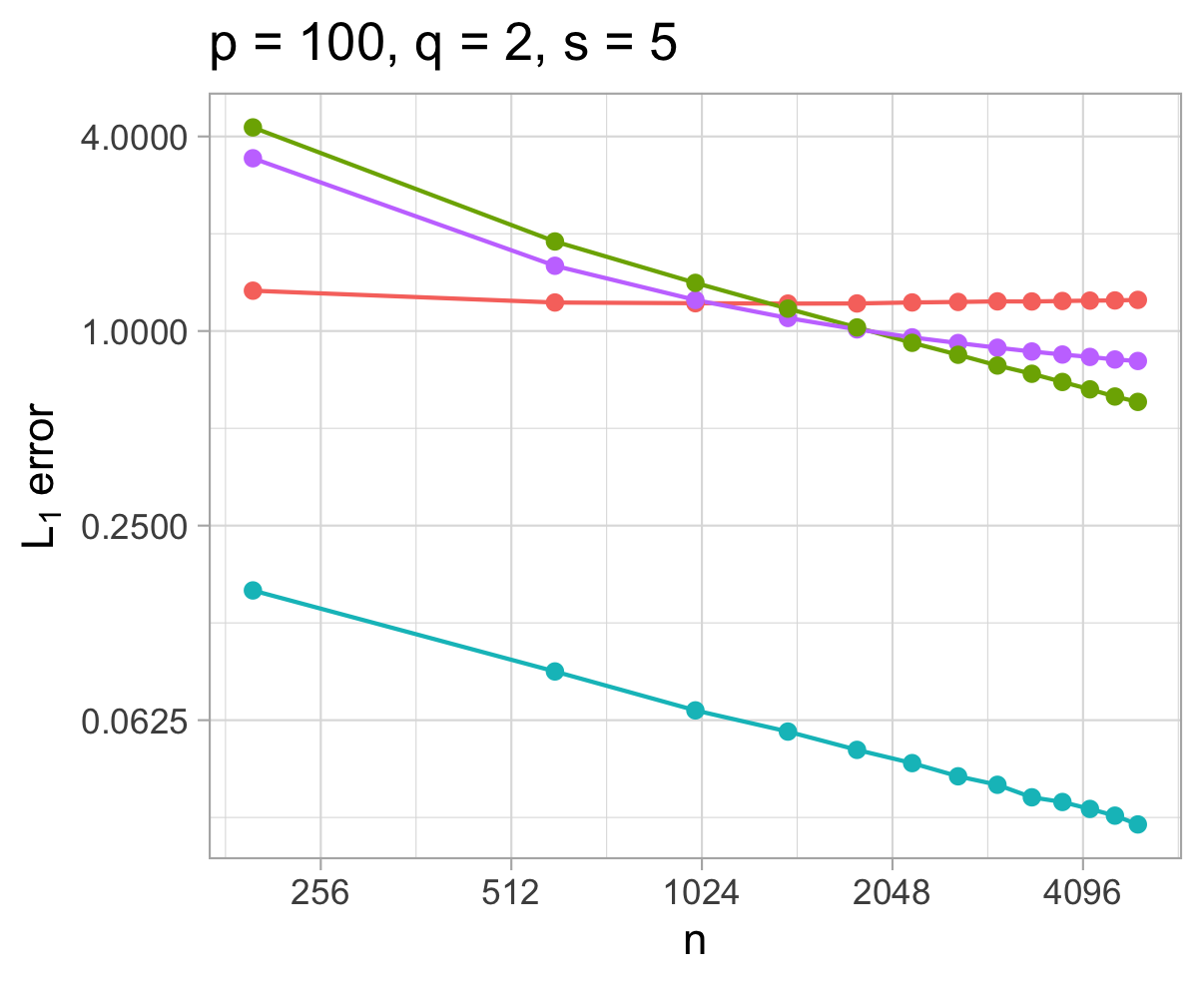
(a) $p=100$, and $n$ varies from $200$ to $5000$.

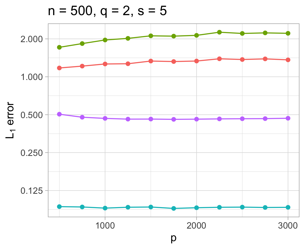
(b) $n=500$, and $p$ varies from $500$ to $3000$.

Figure 2: Estimation errors $||\widehat{\beta}-\beta||_{1}$ for SIV (blue), Lasso (red), Trim (purple), and Null (green) based on $1000$ Monte Carlo runs.

We present the $\ell_{1}$-estimation errors of the four methods in Figures 2(a) and 2(b). For low-dimensional cases, from Figure 2(a), one can see that the Lasso and Trim methods have similar performance in that the bias stabilizes when the sample size is sufficiently large. Both our method and the Null method appear consistent, but the Null method has a much larger bias compared to ours.

For simulation results in the high-dimensional settings, we can see from Figure 2(b) that our SIV method still consistently outperforms the comparison methods. As discussed in Section 1, the true correlations between $X$ and $Y$ are non-sparse. This explains the large estimation errors of the Lasso method. The Null method has even larger biases than the Lasso method. The Trim method was designed specifically for high-dimensional settings, so it is not surprising to see that it outperforms both the Lasso and the Null methods. However, our estimator still enjoys a much smaller bias compared to the Trim estimator.

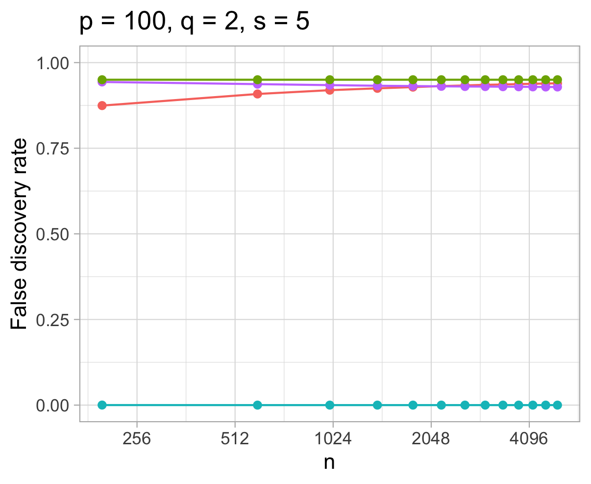
(a) $p=100$, and $n$ varies from $200$ to $5000$.

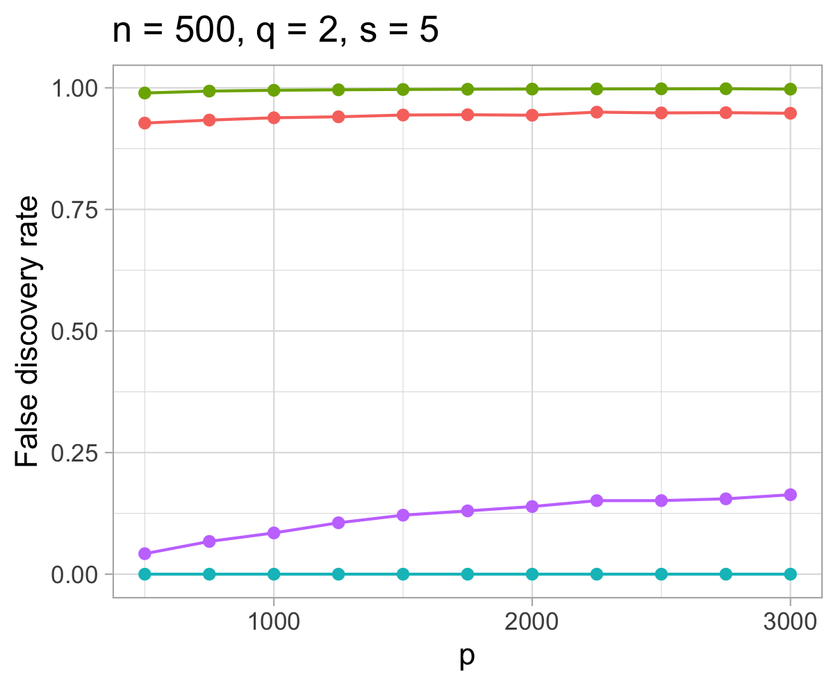
(b) $n=500$, and $p$ varies from $500$ to $3000$.

Figure 3: False discovery rate for SIV (blue), Lasso (red), Trim (purple), and Null (green) based on $1000$ Monte Carlo runs.

Since the underlying $\beta$ is sparse, we also report the performance of variable selection for all the methods in Figures 3(a) and 3(b). All these methods classify the true causes of the outcome as active exposures, that is, $\widehat{\mathcal{A}}\supseteq\mathcal{A}$. Thus we only report the average of the false discovery rates, denoted as $\#\{\widehat{\mathcal{A}}\setminus\mathcal{A}\}/\#\widehat{\mathcal{A}}$, among 1000 Monte Carlo runs. It is easy to see that our proposal has the lowest false discovery rate among all the methods in both the low- and high-dimensional settings.

5.2 Simulation for testing identifiability

Algorithm 2 can also be used to test the identifiability of $\beta$. To evaluate its performance, we consider the following simulation setting. We let $p=8$, $q=2$, and $n=5000$. The $\Lambda_{j,k}$, $\gamma_{k}$, $U_{i,k}$, $\epsilon_{x}$, and $\epsilon_{y}$ are generated in the same way as in the previous subsection. We consider $s=1,2,\ldots,8$. We set $\beta_{1}=\beta_{2}=\ldots\beta_{s}=1$ and $\beta_{s+1}=\ldots=\beta_{p}=0$. In these settings, based on the results in Theorem 2, $\beta$ is identifiable when $s\leq 5$ and not identifiable when $s\geq 6$.

In Figure 4, we report the frequency that the SIV procedure specified in Algorithm 2 outputs that $\beta$ is not identifiable. When $s\leq 5$, our procedure agrees in most cases that the parameter is identifiable. When $s$ increases to $6$, our proposal can indicate the parameters are no longer identifiable with a high probability. This simulation result suggests our procedure can help to test the identifiability of the parameters.

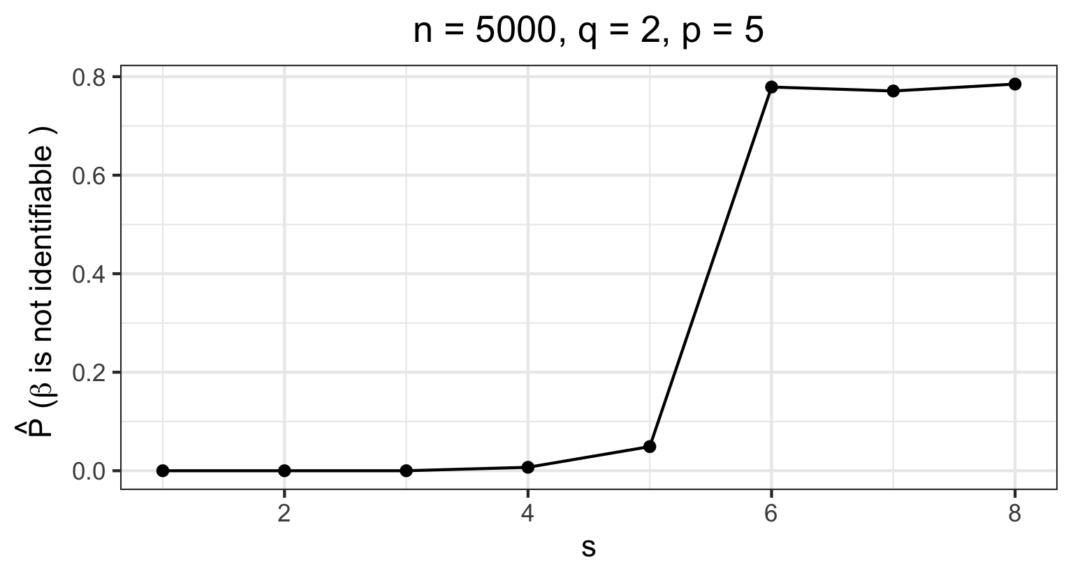
Figure 4: Frequency that the SIV method outputs that the parameter $\beta$ is not-identifiable. In this simulation setting, $p=8$, $q=2$, and $n=5000$, under which $\beta$ is identifiable for $s=1,\ldots,5$, and not identifiable for $s=6,7,8.$

6 Real data application

To further illustrate the proposed synthetic instrumental variable method, we reanalyzed a mouse obesity dataset described by Wang et al. (2006). The study includes a cross of 334 mice between C3H and the susceptible strain C57BL/6J (B6) on an ApoE–null background, which were fed a Western diet for 16 weeks. Data collected on these mice include genotype data on 1327 SNPs, gene expressions of the liver tissues for 23,388 genes, and clinical information such as body weights. Lin et al. (2015) previously analyzed this dataset using regularized methods for high-dimensional instrumental variables regression. Specifically, they treat the SNPs as potential instruments, the gene expressions as treatments, and select 17 genes that are likely to affect the outcome, which is mouse body weight; see also Gleason et al. (2021) for controversies on using SNPs as instruments for estimating the effects of gene expression. Miao et al. (2022) applied their method to estimate the causal effects associated with these 17 genes. Note their method cannot be applied to estimate the effects associated with the 23,388 genes in the original dataset, as their framework only accommodates low-dimensional exposures. In our data analysis, we shall use the same dataset to identify the genes that affect mouse body weight and estimate the sizes of these effects. Note our method does not rely on the collection of the genotype data or other instrumental variables and can accommodate high-dimensional exposures.

We followed the procedure described in Lin et al. (2015) to pre-process the dataset. Genes with a missing rate greater than 0.1 were removed, and the remaining missing gene expression data were imputed using the nearest neighbor averaging (Troyanskaya et al., 2001). We also removed genes that cannot be mapped into Mouse Genome Database (MGD) and have a standard deviation of gene expression levels less than $0.1$. We fitted a marginal linear regression model between mice’s body weight and sex to subtract the estimated sex effect from the body weight to adjust for the effect of sex. We used the fitted residual as outcome $Y$ and centered and standardized gene expression levels as multiple treatments. After data cleaning and merging gene expression and clinical data, a dataset with $p=2819$ genes on $n=306$ mice ($154$ female and $152$ male) is produced.

The statistical test proposed by Onatski (2009) suggests that there are three unobserved latent factors, so we applied our method with $\widehat{q}=3$. Five genes were found to affect the mouse body weight. Under the plurality rule A4, we conclude that the causal effects are identifiable as $\widehat{q}+\widehat{s}=8\ll p=2819$. Specifically, our analysis results suggest that increasing the gene expression levels of $Igfbp2$, $Rab27a$, $Dct$, $Ankhd1$, and $Gck$ by one standard deviation leads to a change of $-1.98$, $1.88$, $1.43$, $-1.33$, and $1.17$ grams in mouse body weight, respectively.

We compare our approach with three methods: (i) the Lasso method; (ii) the two-stage regularization (2SR) method (Lin et al., 2015), where they leverage the SNPs as high-dimensional instrumental variables to estimate the causal effect; (iii) the auxiliary variable method (Miao et al., 2022), where they focus on the $17$ genes deemed by Lin et al. (2015) to have non-zero effects and use the five SNPs selected by Lin et al. (2015) as auxiliary variables; (iv) the null variable method (Miao et al., 2022), where they assume more than half of the $17$ genes have zero effects on mouse body weight; (v) the Trim method (Ćevid et al., 2020). The detailed results of these comparison methods are included in the supplementary material Section F. The number of active genes found by these methods, defined as genes that have non-zero effects on mouse body weight, is 87, 17, 4, 2, and 4, respectively. Similar to the simulation results, the Lasso method identifies much more active exposures than ours, and their selected set of active genes includes those selected by our method. Compared to the other methods, both the 2SR and auxiliary variable methods rely on additional SNP information. All the methods, except for the null variable method, identify the expression of the $Igfbp2$ (insulin-like growth factor binding protein 2) gene as a cause of obesity, which is known to prevent the development of obesity and protect against insulin resistance (Wheatcroft et al., 2007). In addition to $Igfbp2$, we also identify four other genes as potential contributors to obesity. The $Rab27a$ (Ras-related protein Rab-27A) gene functions in docking insulin granules to the pancreatic $\beta$ cell plasma membrane. Scientists have observed that Rab27a-mutated mice exhibit glucose intolerance after a glucose load (Kasai et al., 2005), which might explain its positive effect on body weight. The gene $Dct$ (Dopachrome Tautomerase) has been reported to affect obesity and glucose intolerance (Kim et al., 2015), and it has been detected that $Dct$ overexpresses in visceral adipose tissue of morbidly obese patients (Randhawa et al., 2009). The $Gck$ (Glucokinase) is a gene that plays an important role in recognizing the blood glucose level in the body. It has been reported that overexpression of $Gck$ leads to insulin resistance (Randhawa et al., 2009), which explains its positive effect on body weight.

7 Discussion

In this paper, we study how to identify and estimate the causal effects with a multi-dimensional treatment in the presence of unmeasured confounding. Our key assumption is a sparse causation assumption, which in many contexts, serves as an appealing alternative to the widely-adopted sparse association assumption. We develop a synthetic instrument approach to identify and estimate the causal effects, without the need for collecting additional exogenous information such as the instrumental variables. Under the linear structural equation models, our estimation procedure can be formulated as an $\ell_{0}$-optimization problem and hence can be solved efficiently using off-the-shelf packages.

We have focused our discussions under the framework of linear structural equation models, as it provides a “useful microscope” for causal analysis (Pearl, 2013). Our approach may be extended beyond linear models. Our identification approach leading to Theorem 2 still applies in the non-linear case, as both the voting analogy presented in Table 1 and the plurality condition A4 are independent of the linearity assumption. The extension of our estimation procedure is more involved. In cases where the relationship between the latent confounder $U$ and the treatment $X$ is non-linear, one may need to perform a non-linear factor analysis instead (Yalcin and Amemiya, 2001). When the outcome model is non-linear, the standard two-stage least squares estimator may be biased (e.g. Wan et al., 2018), so one has to rely on alternative methods for estimating the causal effects with instrumental variables (e.g. Wang et al., 2022). These extensions are beyond the scope of our current paper and will be left for future research.

We have also focused on the identification and estimation problems in this paper. Assuming that the $\ell_{0}$-penalization procedure (8) accurately selects the true non-zero causal effects, standard M-estimation theory can be used to construct point-wise confidence intervals. On the other hand, it remains a challenge to construct uniformly valid confidence intervals for the causal parameters, as statistical inference after model selection is typically not uniform (Leeb and Pötscher, 2005). One promising approach is to build on a uniformly valid inference method for the standard $\ell_{0}$-penalization procedure, which to the best of our knowledge, remains an open problem in the statistical literature.

References

- Anderson and Rubin (1956) Anderson, T. and Rubin, H. (1956), “Statistical inference in factor analysis,” in Proceedings of the Third Berkeley Symposium on Mathematical Statistics and Probability: Held at the Statistical Laboratory, University of California, December, 1954, July and August, 1955, Univ of California Press, vol. 1, p. 111.
- Angrist et al. (1996) Angrist, J. D., Imbens, G. W., and Rubin, D. B. (1996), “Identification of causal effects using instrumental variables,” Journal of the American Statistical Association, 91, 444–455.
- Bai (2003) Bai, J. (2003), “Inferential theory for factor models of large dimensions,” Econometrica, 71, 135–171.
- Bing et al. (2022) Bing, X., Ning, Y., and Xu, Y. (2022), “Adaptive estimation in multivariate response regression with hidden variables,” The Annals of Statistics, 50, 640–672.
- Ćevid et al. (2020) Ćevid, D., Bühlmann, P., and Meinshausen, N. (2020), “Spectral deconfounding via perturbed sparse linear models,” Journal of Machine Learning Research (JMLR), 21, 1–41.
- Chandrasekaran et al. (2010) Chandrasekaran, V., Parrilo, P. A., and Willsky, A. S. (2010), “Latent variable graphical model selection via convex optimization,” in 2010 48th Annual Allerton Conference on Communication, Control, and Computing (Allerton), IEEE, pp. 1610–1613.
- Claassen et al. (2013) Claassen, T., Mooij, J., and Heskes, T. (2013), “Learning sparse causal models is not NP-hard,” arXiv preprint arXiv:1309.6824.
- D’Amour (2019) D’Amour, A. (2019), “On multi-cause approaches to causal inference with unobserved counfounding: Two cautionary failure cases and a promising alternative,” in The 22nd International Conference on Artificial Intelligence and Statistics, PMLR, pp. 3478–3486.
- Fan et al. (2013) Fan, J., Liao, Y., and Mincheva, M. (2013), “Large covariance estimation by thresholding principal orthogonal complements,” Journal of the Royal Statistical Society: Series B (Statistical Methodology), 75, 603–680.
- Gleason et al. (2021) Gleason, K. J., Yang, F., and Chen, L. S. (2021), “A robust two-sample transcriptome-wide Mendelian randomization method integrating GWAS with multi-tissue eQTL summary statistics,” Genetic Epidemiology, 45, 353–371.
- Guo et al. (2022) Guo, Z., Ćevid, D., and Bühlmann, P. (2022), “Doubly debiased lasso: High-dimensional inference under hidden confounding,” Annals of Statistics, 50, 1320–1347.
- Guo et al. (2018) Guo, Z., Kang, H., Tony Cai, T., and Small, D. S. (2018), “Confidence intervals for causal effects with invalid instruments by using two-stage hard thresholding with voting,” Journal of the Royal Statistical Society: Series B (Statistical Methodology), 80, 793–815.
- Han and Wang (2013) Han, P. and Wang, L. (2013), “Estimation with missing data: beyond double robustness,” Biometrika, 100, 417–430.
- Hastie et al. (2009) Hastie, T., Tibshirani, R., Friedman, J. H., and Friedman, J. H. (2009), The elements of statistical learning: data mining, inference, and prediction, vol. 2, Springer.
- Kang et al. (2016) Kang, H., Zhang, A., Cai, T. T., and Small, D. S. (2016), “Instrumental variables estimation with some invalid instruments and its application to Mendelian randomization,” Journal of the American Statistical Association, 111, 132–144.
- Kanwal et al. (2017) Kanwal, M., Ding, X.-J., and Cao, Y. (2017), “Familial risk for lung cancer,” Oncology Letters, 13, 535–542.
- Kasai et al. (2005) Kasai, K., Ohara-Imaizumi, M., Takahashi, N., Mizutani, S., Zhao, S., Kikuta, T., Kasai, H., Nagamatsu, S., Gomi, H., Izumi, T., et al. (2005), “Rab27a mediates the tight docking of insulin granules onto the plasma membrane during glucose stimulation,” The Journal of Clinical Investigation, 115, 388–396.
- Kim et al. (2015) Kim, B.-S., Pallua, N., Bernhagen, J., and Bucala, R. (2015), “The macrophage migration inhibitory factor protein superfamily in obesity and wound repair,” Experimental & Molecular Medicine, 47, e161–e161.
- Kong et al. (2022) Kong, D., Yang, S., and Wang, L. (2022), “Identifiability of causal effects with multiple causes and a binary outcome,” Biometrika, 109, 265–272.
- Leeb and Pötscher (2005) Leeb, H. and Pötscher, B. M. (2005), “Model selection and inference: Facts and fiction,” Econometric Theory, 21, 21–59.
- Lin et al. (2015) Lin, W., Feng, R., and Li, H. (2015), “Regularization methods for high-dimensional instrumental variables regression with an application to genetical genomics,” Journal of the American Statistical Association, 110, 270–288.
- Miao et al. (2022) Miao, W., Hu, W., Ogburn, E. L., and Zhou, X.-H. (2022), “Identifying effects of multiple treatments in the presence of unmeasured confounding,” Journal of the American Statistical Association, 1–15.
- Ogburn et al. (2020) Ogburn, E. L., Shpitser, I., and Tchetgen, E. J. T. (2020), “Counterexamples to ‘the blessings of multiple causes’ by Wang and Blei,” arXiv preprint arXiv:2001.06555.
- Onatski (2009) Onatski, A. (2009), “A formal statistical test for the number of factors in the approximate factor models,” Econometrica, 77, 1447–1480.
- Pearl (2013) Pearl, J. (2013), “Linear models: A useful ‘microscope’ for causal analysis,” Journal of Causal Inference, 1, 155–170.
- Randhawa et al. (2009) Randhawa, M., Huff, T., Valencia, J. C., Younossi, Z., Chandhoke, V., Hearing, V. J., and Baranova, A. (2009), “Evidence for the ectopic synthesis of melanin in human adipose tissue,” The FASEB Journal, 23, 835–843.
- Raskutti et al. (2011) Raskutti, G., Wainwright, M. J., and Yu, B. (2011), “Minimax rates of estimation for high-dimensional linear regression over -balls,” IEEE Transactions on Information Theory, 57, 6976–6994.
- Shen et al. (2016) Shen, D., Shen, H., and Marron, J. (2016), “A general framework for consistency of principal component analysis,” The Journal of Machine Learning Research, 17, 5218–5251.
- Shen et al. (2013) Shen, X., Pan, W., Zhu, Y., and Zhou, H. (2013), “On constrained and regularized high-dimensional regression,” Annals of the Institute of Statistical Mathematics, 65, 807–832.
- Spirtes and Glymour (1991) Spirtes, P. and Glymour, C. (1991), “An algorithm for fast recovery of sparse causal graphs,” Social Science Computer Review, 9, 62–72.
- Sun et al. (2023) Sun, B., Liu, Z., and Tchetgen, E. T. (2023), “Semiparametric Efficient G-estimation with Invalid Instrumental Variables,” Biometrika.
- Tchetgen et al. (2020) Tchetgen, E. J. T., Ying, A., Cui, Y., Shi, X., and Miao, W. (2020), “An introduction to proximal causal learning,” arXiv preprint arXiv:2009.10982.
- Tibshirani (1996) Tibshirani, R. (1996), “Regression shrinkage and selection via the lasso,” Journal of the Royal Statistical Society: Series B (Methodological), 58, 267–288.
- Troyanskaya et al. (2001) Troyanskaya, O., Cantor, M., Sherlock, G., Brown, P., Hastie, T., Tibshirani, R., Botstein, D., and Altman, R. B. (2001), “Missing value estimation methods for DNA microarrays,” Bioinformatics, 17, 520–525.
- Wan et al. (2018) Wan, F., Small, D., and Mitra, N. (2018), “A general approach to evaluating the bias of 2-stage instrumental variable estimators,” Statistics in Medicine, 37, 1997–2015.
- Wang et al. (2017) Wang, J., Zhao, Q., Hastie, T., and Owen, A. B. (2017), “Confounder adjustment in multiple hypothesis testing,” Annals of Statistics, 45, 1863.
- Wang and Tchetgen Tchetgen (2018) Wang, L. and Tchetgen Tchetgen, E. (2018), “Bounded, efficient and multiply robust estimation of average treatment effects using instrumental variables,” Journal of the Royal Statistical Society: Series B (Statistical Methodology), 80, 531–550.
- Wang et al. (2022) Wang, L., Tchetgen Tchetgen, E., Martinussen, T., and Vansteelandt, S. (2022), “Instrumental variable estimation of the causal hazard ratio,” Biometrics.
- Wang et al. (2006) Wang, S., Yehya, N., Schadt, E. E., Wang, H., Drake, T. A., and Lusis, A. J. (2006), “Genetic and genomic analysis of a fat mass trait with complex inheritance reveals marked sex specificity,” PLOS Genetics, 2, e15.
- Wang and Blei (2019) Wang, Y. and Blei, D. M. (2019), “The blessings of multiple causes,” Journal of the American Statistical Association, 114, 1574–1596.
- Wheatcroft et al. (2007) Wheatcroft, S. B., Kearney, M. T., Shah, A. M., Ezzat, V. A., Miell, J. R., Modo, M., Williams, S. C., Cawthorn, W. P., Medina-Gomez, G., Vidal-Puig, A., et al. (2007), “IGF-binding protein-2 protects against the development of obesity and insulin resistance,” Diabetes, 56, 285–294.
- Yalcin and Amemiya (2001) Yalcin, I. and Amemiya, Y. (2001), “Nonlinear factor analysis as a statistical method,” Statistical Science, 275–294.
- Zhou et al. (2009) Zhou, X.-H., McClish, D. K., and Obuchowski, N. A. (2009), Statistical methods in diagnostic medicine, John Wiley & Sons.
- Zhou et al. (2020) Zhou, Y., Tang, D., Kong, D., and Wang, L. (2020), “The Promises of Parallel Outcomes,” arXiv preprint arXiv:2012.05849.