Global Momentum Estimation of
an Electric Power System

Abstract

This work presents a technique to estimate on-line the global momentum of an electric power system. It exploits the footprint of the principal frequency system dynamics. Probing tones are injected by a grid-forming converter-interfaced generator and the speed of its virtual rotor is exploited to extrapolate the footprint. The proposed technique is entirely data driven and thus it does not need any model of the power system. We show that the proposed technique is adequate to accurately estimate the actual global momentum contributed by synchronous machines and provided by the controllers of converter-interfaced generators that emulate the behavior of synchronous machines. The technique is comprehensively tested on a modified version of the ieee 39-bus system and a dynamic version of the ieee 118-bus system, containing grid forming converter interfaced generators.

I Introduction

I-A Motivation

From the beginning of this century, the importance of estimating an electric power grid’s available inertia—or better yet, its momentum—has been steadily increasing. To a large extent, this explains the large amount of papers on this topic that one can find in the scientific literature. The interested reader can find the motivations supporting this trend in the introductions of those contributions and, in particular, in extensive review papers such as [1, 2].

I-B Literature Review

The literature concerning inertia estimation in power systems is vast and has been growing at a quickening pace. Limited to the “Scopus” abstract and citation database of peer-reviewed papers, papers including the keywords “inertia” and “power system” in their abstract were only $\displaystyle 30$ in $\displaystyle 2000$, while this figure spiked to $\displaystyle 1200$ in $\displaystyle 2022$: nevertheless, the problem is still open, despite the untiring work of numerous research groups.

In this context, we present a reliable and efficient method for estimating online the global momentum available in a power system. The method belongs to the class of algorithms based on active perturbations, where proper probing signals[3] are used for system identification purposes[4, 5].

Focusing on this class of approaches, the method proposed in [6] was verified in an actual power system and resulted effective for small-scale islanded systems. In [7], a power system was probed by small active power changes through an energy storage system that did not impact the operational stability of the system. The goal was to provide the energy storage system operators with a tool to estimate the unknown time-varying inertia of any generic power system and properly tune/control their devices for fast-frequency strategies. Low-level probing signals were used also in [8] for accurate estimation of inertia and damping constants in microgrids by resorting to a moving horizon estimation approach. The method proposed in [9] is possibly the most well-known in the considered class. The authors proposed a closed-loop identification technique to estimate the equivalent inertia constant of a power system at the connection bus. The method aims to estimate the inertia constant of a single device connected to the grid.

The method we propose has a wider scope since it allows to estimate online the global momentum of large-size realistic power system. The main source of inspiration for our work was the activity conducted by other researchers in the realm of frequency synchronization of power generators. The latter is a necessary condition for the operation of power-grid networks. During steady operation, the frequency is the same throughout the entire power grid and any pair of generators has a fixed phase difference that determines the power flows. Even if the focus of our work is not synchronization but global momentum estimation, the main results we propose are grounded on this concept. It is thus worth mentioning that one can find in the literature many contributions on synchronization (see for instance [10, 11, 12, 13, 14, 15, 16]).

I-C Contribution

Here, we provide a theoretical framework based on the dynamic response of a generic power system model containing synchronous generators equipped with primary frequency control and grid-forming (gf) converter-interfaced generators whose swing equations are described by the classical model [17, 18]. By interpreting the power system as a power-controlled oscillator whose instantaneous oscillation frequency is controlled by the power flows, we derive the analytical expression in the frequency domain of the principal frequency system dynamics. We show that this expression represents the behavior shared by the rotor speed of all the synchronous generators and thus also by gf cig elements present in the grid, provided that a proper amount of synchronization (at low frequencies) is guaranteed between these devices. One of the parameters of this expression is the global momentum of the grid, which can thus be estimated with appropriate identification techniques. We show that the estimation depends neither on the electrical characteristics of the interconnecting lines, nor on the number of buses, controllers, governors, and synchronous machine models but only on the collected data, i.e., the proposed estimation method is agnostic with respect to the system.

Based on these considerations, we exploit a gf cig that is either already present in the power system, or can be inserted with the specific purpose of allowing the estimation of the power system global momentum. The probing signals used to stimulate the power system in a suitable frequency band are injected by the gf cig and its virtual rotor speed is sampled at an appropriate rate. By resorting to the vector fitting (vf) technique [19, 20, 21], we obtain the parameters that provide the best fit of the analytical expression of the frequency spectrum of the collected samples. The global momentum of the power system is among these parameters.

I-D Organization

In Sec. II we present the theoretical foundation of the proposed method. In Sec. III, through a basic case-study, we highlight how the global momentum of the power system can be identified in the low-frequency spectrum expression of the rotor speed of all the synchronous generators and gf cig elements that are present in the grid. The general formulation of the method is given in Sec. IV. Finally, in Sec. V we verify the validity of the proposed approach in the ieee 39-bus and ieee 118-bus power system models.

II The Power System as a Power-Controlled Oscillator

In electronics, a voltage-controlled oscillator is an oscillator whose oscillation frequency is controlled by a voltage input: the applied voltage determines the instantaneous oscillation frequency. Analogously, a generic power system can be viewed as a power-controlled oscillator whose instantaneous oscillation frequency, i.e., rotor speed of synchronous generators, is controlled by the power flows.

In an autonomous oscillator, steady-state periodic solutions lack a phase reference [22, 23]. Even if a limit cycle is unique and isolated in the phase space, two orbits originating from two different initial conditions belonging to this limit cycle will remain shifted in the time domain. This property is at the origin of phase noise in electronic oscillators [24]. From the viewpoint of dynamical systems theory, according to Floquet’s theory, this is justified by the presence of a characteristic multiplier equal to $\displaystyle 1$.

The same holds in power systems where a stationary solution is not an isolated equilibrium but is embedded in a continuum of equilibria [25]. When the power system is modeled in the dq-frame, the presence of a characteristic multiplier equal to $\displaystyle 1$ corresponds to a eigenvalue equal to $\displaystyle 0$ in the Jacobian matrix of the power system model linearized around an equilibrium point [26]. Indeed, the classical power system model aims at representing the envelope of the actual system dynamics through a steady-state solution. In other words, the periodic steady-state solution at the fundamental frequency with a constant envelope is actually represented as a constant steady-state solution playing the role of a stationary solution in the dq-frame.

In reality, the power system model is more complex than a voltage-controlled oscillator since it is made up of several power-controlled oscillators (viz., synchronous generators and gf cigs) [10, 15]. An overall instantaneous oscillation frequency, shared by all of these components, is observed only when these local and interconnected oscillators are synchronized. In practice, even in normal operating conditions, it never occurs but on average. As a matter of fact, the power system model never works at steady state because of random fluctuations in the power consumption of the loads or in the energy production of renewable energy sources.

To clarify these concepts, it is useful to discuss what happens in a power system model including $\displaystyle N$ synchronous generators whose dynamic evolution is modeled by the simple swing equation and equipped with primary frequency control. Generators are interconnected by lines and transformers, and constant-power and/or constant-impedance loads are connected to the grid buses. Under these assumptions, the overall power system model is described by the following set of $\displaystyle 3N$ ordinary differential equations,

$${\boldsymbol{\dot{\delta}}} =\Omega\left(\boldsymbol{\omega}-\omega_{0}\right)$$ (1)

$$\boldsymbol{{\mathcal{M}}}\boldsymbol{\dot{\omega}} =\boldsymbol{P}_{m}-\boldsymbol{P}_{e}(\boldsymbol{\delta})-\boldsymbol{{\mathcal{D}}}(\boldsymbol{\omega}-\omega_{0})$$

$$\boldsymbol{T}_{g}\boldsymbol{\dot{P}}_{m} =\boldsymbol{P}_{{m_{\mathrm{eq}}}}-\boldsymbol{P}_{m}-{\boldsymbol{k}_{g}}{\boldsymbol{R}^{-1}}(\boldsymbol{\omega}-\omega_{0})~{},$$

where the meaning of symbols in (1) is as follows:

• $\displaystyle\Omega$: the base synchronous frequency in $\displaystyle\rad/\mathrm{s}$;

• $\displaystyle\boldsymbol{\omega}(t)\in\mathds{R}^{N}$: the per-unit rotor speeds of the machines;

• $\displaystyle\omega_{0}\in\mathds{R}$: the per-unit reference synchronous frequency;

• $\displaystyle\boldsymbol{\delta}(t)\in\mathds{R}^{N}$: the rotor angles of the machines;

• $\displaystyle{\boldsymbol{{\mathcal{M}}}\in\mathds{R}^{N\times N}}$: a diagonal matrix whose $\displaystyle j$-th element is the product of the inertia constant $\displaystyle H_{j}$ and the rated power $\displaystyle S_{B_{j}}$ of the $\displaystyle j$-th machine: $\displaystyle\mathcal{M}_{jj}=2H_{j}S_{B_{j}}$ for $\displaystyle{j=1,\dots,N}$;

• $\displaystyle{\boldsymbol{{\mathcal{D}}}\in\mathds{R}^{N\times N}}$: a diagonal matrix whose $\displaystyle j$-th element is the product of the load damping factor $\displaystyle D_{j}$ and the rated power $\displaystyle S_{B_{j}}$ of the $\displaystyle j$-th machine: $\displaystyle{\mathcal{D}}_{jj}=D_{j}S_{B_{j}}$ for $\displaystyle{j=1,\dots,N}$;

• $\displaystyle\boldsymbol{P}_{e}(\boldsymbol{\delta})\in\mathds{R}^{N}$: the electrical active power exchanged by the machines;

• $\displaystyle{\boldsymbol{P}_{m}}\in\mathds{R}^{N}$: the mechanical power of the machines, governed by their prime mover;

• $\displaystyle{\boldsymbol{P}_{m_{\mathrm{eq}}}}\in\mathds{R}^{N}$: the mechanical power setpoint of the machines corresponding to the power flow solution;

• $\displaystyle{\boldsymbol{T}_{g}}$, $\displaystyle{\boldsymbol{k}_{g}}$, $\displaystyle{\boldsymbol{R}}\in\mathds{R}^{N\times N}$: the diagonal matrices whose elements model the time constant, gain constant, and droop gain of the primary frequency controls, respectively.

It is worth noticing that the first set of $\displaystyle N$ odes in (1) should be written as $\displaystyle{\boldsymbol{\dot{\delta}}}=\Omega\boldsymbol{\omega}$ if one wanted to completely retain the formulation in polar coordinates of the synchronous-generator dynamical equations, in which the rotor angle grows unbounded since the rotor keeps rotating. Nevertheless, (1) is usually adopted to identify an equilibrium point of the system, say $\displaystyle[\boldsymbol{\delta}_{\mathrm{eq}}^{\mathrm{T}},\boldsymbol{\omega}_{\mathrm{eq}}^{\mathrm{T}},\boldsymbol{P}_{m_{\mathrm{eq}}}^{\mathrm{T}}]^{\mathrm{T}}$, neglecting the common shifting evolution of the $\displaystyle{\boldsymbol{\delta}}$ rotor angles.

Given a common shift of the $\displaystyle{\boldsymbol{\delta}}$ rotor angles written as $\displaystyle{\boldsymbol{\delta}(t)+\alpha(t)}$, where $\displaystyle\alpha(t)$ is a scalar function, we have that $\displaystyle{\boldsymbol{P}_{e}(\boldsymbol{\delta}(t)+\alpha(t))=\boldsymbol{P}_{e}(\boldsymbol{\delta}(t))}$. As a consequence, by considering the linearisation of (1) we have

$$\left[\!\!\begin{array}[]{c}\Delta\boldsymbol{\dot{\delta}}\\ \Delta\boldsymbol{\dot{\omega}}\\ \Delta\boldsymbol{\dot{P}}_{m}\\ \end{array}\!\!\right]\!\!=\!\!\underbrace{\left[\!\!\!\!\begin{array}[]{c c c}\boldsymbol{\mathbbm{O}}_{N}&\Omega\boldsymbol{\mathbbm{1}}_{N}&\boldsymbol{\mathbbm{O}}_{N}\\ -\boldsymbol{{\mathcal{M}}}^{-1}\boldsymbol{\Pi}&-\boldsymbol{{\mathcal{M}}}^{-1}\boldsymbol{{\mathcal{D}}}&\boldsymbol{{\mathcal{M}}}^{-1}\\ \boldsymbol{\mathbbm{O}}_{N}&-\boldsymbol{T}^{-1}_{g}\boldsymbol{k}_{g}\boldsymbol{R}^{-1}&-\boldsymbol{T}^{-1}_{g}\\ \end{array}\!\!\!\!\right]}_{\boldsymbol{A}}\!\!\left[\!\!\begin{array}[]{c}\Delta\boldsymbol{\delta}\\ \Delta\boldsymbol{\omega}\\ \Delta\boldsymbol{P}_{m}\\ \end{array}\!\!\right]~{},$$ (2)

where the $\displaystyle\boldsymbol{\Pi}=\frac{\partial{\boldsymbol{P}_{e}}}{\partial\boldsymbol{\delta}}$ matrix is the network interconnection Laplacian singular matrix [27] and $\displaystyle\boldsymbol{\Pi}=\boldsymbol{\Pi}^{\mathrm{T}}$. The null space of $\displaystyle\boldsymbol{\Pi}$ is spanned by $\displaystyle\ker(\boldsymbol{\Pi})=\boldsymbol{\mathbbm{1}}_{N,1}$. The $\displaystyle\boldsymbol{A}$ matrix is thus singular too and $\displaystyle\ker(\boldsymbol{A})\equiv\boldsymbol{u}_{1}=[\boldsymbol{\mathbbm{1}}_{1,N},\boldsymbol{\mathbbm{O}}_{1,2N}]^{\mathrm{T}}$.

When a small-signal $\displaystyle{\boldsymbol{b}(t)\in\mathbb{R}^{N}}$ is added to $\displaystyle\boldsymbol{P}_{e}(\boldsymbol{\delta}(t))$, thus emulating the injection of (stochastic) disturbances or probing signals, the $\displaystyle N$ odes in (1) governing $\displaystyle{\boldsymbol{\dot{\omega}}}$ become

$$\boldsymbol{{\mathcal{M}}}\boldsymbol{\dot{\omega}}=\boldsymbol{P}_{m}-\boldsymbol{P}_{e}(\boldsymbol{\delta})-\boldsymbol{{\mathcal{D}}}(\boldsymbol{\omega}-\omega_{0})+\boldsymbol{b}(t)~{}.$$ (3)

Since $\displaystyle\boldsymbol{A}$ is singular, it is not possible to exploit (2) to obtain an approximate solution of (3) in the neighborhood of $\displaystyle[\boldsymbol{\delta}_{\mathrm{eq}}^{\mathrm{T}},\boldsymbol{\omega}_{\mathrm{eq}}^{\mathrm{T}},\boldsymbol{P}_{m_{\mathrm{eq}}}^{\mathrm{T}}]^{\mathrm{T}}$. Nevertheless, in this case, the singularity of $\displaystyle\boldsymbol{\Pi}$ is a key aspect to allow resorting to the small-signal formulation to study the perturbed evolution of $\displaystyle\boldsymbol{\omega}(t)=\boldsymbol{\omega}_{\mathrm{eq}}+\Delta\boldsymbol{\omega}(t)$. To explore this aspect, let us define $\displaystyle\boldsymbol{u}_{k}$ and $\displaystyle\boldsymbol{v}_{k}$ as the $\displaystyle 3N$ right and left eigenvectors of $\displaystyle\boldsymbol{A}$, respectively ($\displaystyle\boldsymbol{u}_{1}$ and $\displaystyle\boldsymbol{v}_{1}$ are associated to the $\displaystyle\lambda_{1}=0$ eigenvalue). So doing we are assuming that $\displaystyle\boldsymbol{A}$ has distinct eigenvalues (their value is related to the eigenvalues of $\displaystyle\boldsymbol{\Pi}$ [27] and to the primary frequency control time-constants) and it is diagonalizable.

Having in mind that, because of the bi-orthogonality property of eigenvectors (i.e., $\displaystyle{\boldsymbol{v}_{k}^{\mathrm{T}}\boldsymbol{u}_{j}\neq 0}$ only if $\displaystyle k\neq j$), it is always possible to write

$$\left[\!\!\!\!\begin{array}[]{c}\boldsymbol{\mathbbm{O}}_{N,1}\\ \boldsymbol{{\mathcal{M}}}^{-1}\boldsymbol{b}(t)\\ \boldsymbol{\mathbbm{O}}_{N,1}\end{array}\!\!\!\!\right]=\underbrace{\boldsymbol{v}_{1}^{\mathrm{T}}\left[\!\!\!\!\begin{array}[]{c}\boldsymbol{\mathbbm{O}}_{N,1}\\ \boldsymbol{{\mathcal{M}}}^{-1}\boldsymbol{b}(t)\\ \boldsymbol{\mathbbm{O}}_{N,1}\end{array}\!\!\!\!\right]\boldsymbol{u}_{1}}_{\boldsymbol{b}_{\delta}(t)}+\underbrace{\sum_{k=2}^{3N}{\boldsymbol{v}_{k}^{\mathrm{T}}\left[\!\!\!\!\begin{array}[]{c}\boldsymbol{\mathbbm{O}}_{N,1}\\ \boldsymbol{{\mathcal{M}}}^{-1}\boldsymbol{b}(t)\\ \boldsymbol{\mathbbm{O}}_{N,1}\end{array}\!\!\!\!\right]\boldsymbol{u}_{k}}}_{\boldsymbol{b}_{\delta\omega}(t)}~{}.$$ (4)

Since

$$\boldsymbol{v}_{1}=\ker(\boldsymbol{A}^{\mathrm{T}})=\frac{\Omega}{\boldsymbol{\mathbbm{1}}_{1,N}\boldsymbol{\Theta}\boldsymbol{\mathbbm{1}}_{N,1}}\left[\begin{array}[]{c}{\boldsymbol{\mathbbm{1}}_{N,1}\boldsymbol{\Theta}}{\Omega^{-1}}\\ \boldsymbol{{\mathcal{M}}}\boldsymbol{\mathbbm{1}}_{N,1}\\ \boldsymbol{T}_{tg}\boldsymbol{\mathbbm{1}}_{N,1}\end{array}\right]~{},$$ (5)

one obtains

$$\boldsymbol{b}_{\delta}(t)=\frac{\Omega}{\boldsymbol{\mathbbm{1}}_{1,N}\boldsymbol{\Theta}\boldsymbol{\mathbbm{1}}_{N,1}}\left[\begin{array}[]{c}\boldsymbol{\mathbbm{1}}_{1,N}\boldsymbol{b}(t)\boldsymbol{\mathbbm{1}}_{N,1}\\ \boldsymbol{\mathbbm{O}}_{2N,1}\end{array}\right]~{},$$ (6)

where $\displaystyle\boldsymbol{\Theta}=\boldsymbol{{\mathcal{D}}}+\boldsymbol{k}_{g}\boldsymbol{R}_{g}^{-1}$ (see Appendix A for more details on the derivation of $\displaystyle\boldsymbol{v}_{1}$).

The effect of $\displaystyle{\boldsymbol{b}_{\delta}(t)}$ is thus to synchronously shift all the components of $\displaystyle{\boldsymbol{\delta}}$ of the same time-varying quantity

$$\alpha(t)=\Omega\int_{0}^{t}{\frac{\boldsymbol{\mathbbm{1}}_{1,N}\boldsymbol{b}(\tau)}{\boldsymbol{\mathbbm{1}}_{1,N}\boldsymbol{\Theta}\boldsymbol{\mathbbm{1}}_{N,1}}d\tau}~{},$$ (7)

without altering the $\displaystyle{\boldsymbol{\omega}}(t)$ vector since $\displaystyle{\boldsymbol{P}_{e}(\boldsymbol{\delta}(t)+\alpha(t))=\boldsymbol{P}_{e}(\boldsymbol{\delta}(t))}$. If $\displaystyle\mathbbm{1}_{1,N}\boldsymbol{b}(\tau)$ has a nonzero mean value $\displaystyle\alpha(t)$ would increase unbounded. This would be true even if $\displaystyle\boldsymbol{b}(\tau)$ were a vector of random variables with zero mean and finite variance as the Ornstein-Uhlenbeck (ou) processes typically used to model stochastic variability of power loads [28, 29, 30, 31]. As a matter of fact, $\displaystyle\alpha(t)$ would exhibit unbounded variance [32]. In both cases, the effect of $\displaystyle{\boldsymbol{b}_{\delta}(t)}$ can not be treated as that of a small signal, even being $\displaystyle{\boldsymbol{b}_{\delta}(t)}$ actually small. In the literature this is known as phase noise [24].

In turn, it is possible to compute the effect of $\displaystyle{\boldsymbol{b}_{\delta\omega}(t)}$ by resorting to the small-signal approach since it is easy to verify that $\displaystyle\boldsymbol{v}_{1}^{\mathrm{T}}\boldsymbol{b}_{\delta\omega}(t)\boldsymbol{u}_{1}=0$. This implies that $\displaystyle{\boldsymbol{b}_{\delta\omega}(t)}$ does not produce any effect similar to $\displaystyle\alpha(t)$. In other words, it is not responsible for coherent phase shifting in the entire power system but produces small fluctuations that are different for all the components of $\displaystyle\boldsymbol{\delta}(t)$. The main implication of this result is that, in the presence of a small signal $\displaystyle\boldsymbol{b}_{\delta\omega}(t)$, the power system does not remain synchronized. In other words, it is possible to prove that, in the presence of the small signal $\displaystyle\boldsymbol{b}_{\delta\omega}(t)$, the hypothesis that the power system remain synchronized, viz. $\displaystyle\Delta\omega_{k}(t)\equiv\Delta\omega(t)$ for $\displaystyle{k=1,\dots,N}$ (or, equivalently, $\displaystyle{\boldsymbol{\Delta}\omega(t)=\Delta\omega(t)\boldsymbol{\mathbbm{1}}_{N,1}}$) is inconsistent with the equations governing the power system itself. This can be derived by focusing on the odes governing the dynamics of $\displaystyle\Delta\boldsymbol{\omega}$. We can write

$$\begin{array}[]{l c l}\boldsymbol{{\mathcal{M}}}\Delta\boldsymbol{\dot{\omega}}&\!\!\!=\!\!\!&\Delta\boldsymbol{P}_{m}-\boldsymbol{\Pi}(\alpha(t)\boldsymbol{\mathbbm{1}}_{N,1}+\Delta\boldsymbol{\delta}(t))-\boldsymbol{{\mathcal{D}}}\Delta\boldsymbol{\omega}+\boldsymbol{b}(t)\\[5.69054pt] &\!\!\!=\!\!\!&\Delta\boldsymbol{P}_{m}-\boldsymbol{\Pi}\Delta\boldsymbol{\delta}(t)-\boldsymbol{{\mathcal{D}}}\Delta\boldsymbol{\omega}+\boldsymbol{{\mathcal{M}}}\boldsymbol{b}_{\delta\omega}(t)\\[5.69054pt] &\!\!\!=\!\!\!&\Delta\boldsymbol{P}_{m}-\boldsymbol{\Pi}\int{\Omega\Delta\boldsymbol{\omega}(t)dt}-\boldsymbol{{\mathcal{D}}}\Delta\boldsymbol{\omega}+\boldsymbol{{\mathcal{M}}}\boldsymbol{b}_{\delta\omega}(t)~{},\end{array}$$ (8)

with $\displaystyle\Delta\boldsymbol{\omega}$ evolving in the neighborhood of $\displaystyle\boldsymbol{\omega}_{\mathrm{eq}}$, i.e., of the frequency at the equilibrium point. It is worth noticing that, thanks to the singularity of $\displaystyle\boldsymbol{\Pi}$, the possibly unbounded contribution of $\displaystyle\alpha(t)\boldsymbol{\mathbbm{1}}_{N,1}$ does not affect $\displaystyle\Delta\boldsymbol{\dot{\omega}}$.

Assuming $\displaystyle{\Delta\boldsymbol{\omega}(t)=\Delta\omega(t)\boldsymbol{\mathbbm{1}}_{N,1}}$, $\displaystyle{\Delta\omega(0)=0}$, and $\displaystyle{\Delta\boldsymbol{P}_{m}(0)=\boldsymbol{\mathbbm{O}}_{N,1}}$, equation (8) can be transformed in the $\displaystyle s$-domain as

$$\begin{array}[]{l c l}s{\Delta{\omega}(s)}\boldsymbol{{\mathcal{M}}}\boldsymbol{\mathbbm{1}}_{N,1}\!\!\!&\!\!=\!\!&\!\!\!\Delta\boldsymbol{P}_{m}(s)-\Omega\frac{\Delta\omega(s)}{s}\underbrace{\boldsymbol{\Pi}\boldsymbol{\mathbbm{1}}_{N,1}}_{\boldsymbol{\mathbbm{O}}_{N,1}}+\\[8.53581pt] \!\!\!&\!\!\!\!&\!\!\!-{\Delta{\omega}(s)}\boldsymbol{{\mathcal{D}}}\boldsymbol{\mathbbm{1}}_{N,1}+\boldsymbol{{\mathcal{M}}}\boldsymbol{b}_{\delta\omega}(s)\\[8.53581pt] \!\!\!&\!\!=\!\!&\!\!\!\Delta\boldsymbol{P}_{m}(s)-{\Delta{\omega}(s)}\boldsymbol{{\mathcal{D}}}\boldsymbol{\mathbbm{1}}_{N,1}+\boldsymbol{{\mathcal{M}}}\boldsymbol{b}_{\delta\omega}(s)~{}.\end{array}$$ (9)

Since

$$\Delta\boldsymbol{P}_{m}(s)=-\left(s\boldsymbol{T}_{g}+\boldsymbol{\mathbbm{1}}_{N}\right)^{-1}\boldsymbol{k}_{g}\boldsymbol{R}^{-1}\boldsymbol{\mathbbm{1}}_{N,1}\Delta\omega(s)~{},$$ (10)

we have

$$\boldsymbol{\Xi}\boldsymbol{\mathbbm{1}}_{N,1}\Delta{\omega}(s)=\boldsymbol{{\mathcal{M}}}\boldsymbol{b}_{\delta\omega}(s)~{},$$ (11)

where $\displaystyle{\boldsymbol{\Xi}=s\boldsymbol{{\mathcal{M}}}+\boldsymbol{{\mathcal{D}}}+\left(s\boldsymbol{T}_{g}+\boldsymbol{\mathbbm{1}}_{N}\right)^{-1}\boldsymbol{k}_{g}\boldsymbol{R}^{-1}}$. Being $\displaystyle\boldsymbol{\Xi}$ a diagonal matrix that, generically, does not contain identical elements in its diagonal, it is not possible to have $\displaystyle{\Delta\boldsymbol{\omega}(t)=\Delta\omega(t)\boldsymbol{\mathbbm{1}}_{N,1}}$, thus violating the initial hypothesis.

How is it possible to reconcile this result with the well-known experimental evidence that, at low-frequency, in properly connected power systems, the components of $\displaystyle{\Delta\boldsymbol{\omega}(t)}$ share almost the same frequency spectrum? Let us consider the small perturbation of the so-called principal frequency system dynamics, viz. the frequency that can be defined for the center of inertia (coi) of the system, i.e.,

$$\Delta\omega_{\textsc{coi}}(t)=\frac{\sum_{k=1}^{N}{S_{B_{k}}H_{k}\Delta\omega_{k}(t)}}{\sum_{k=1}^{N}{S_{B_{k}}H_{k}}}~{}.$$ (12)

The ode governing the evolution of $\displaystyle{\Delta\omega_{\textsc{coi}}(t)}$ is derived by combining the odes of the $\displaystyle\Delta\omega_{k}(t)$ as [17]

$$\mathcal{G}_{\mathcal{M}}\Delta{\dot{\omega}}_{\textsc{coi}}=\\ \boldsymbol{\mathbbm{1}}_{1,N}\left(\Delta\boldsymbol{P}_{m}-\Delta\boldsymbol{P}_{e}-\boldsymbol{{\mathcal{D}}}\Delta\boldsymbol{\omega}+\boldsymbol{{\mathcal{M}}}\boldsymbol{b}_{\delta\omega}(t)\right)$$ (13)

where $\displaystyle\mathcal{G}_{\mathcal{M}}=\boldsymbol{\mathbbm{1}}_{1,N}\boldsymbol{{\mathcal{M}}}\boldsymbol{\mathbbm{1}}_{N,1}$.

If we write $\displaystyle\boldsymbol{b}_{\delta\omega}=\boldsymbol{b}_{\delta\omega}^{\mathrm{lf}}+\boldsymbol{b}_{\delta\omega}^{\mathrm{hf}}$, where $\displaystyle\mbox{}^{\mathrm{lf}}$ and $\displaystyle\mbox{}^{\mathrm{hf}}$ stand for low- and high-frequency, respectively, and $\displaystyle\boldsymbol{b}_{\delta\omega}^{\mathrm{lf}}$ is assumed to generate $\displaystyle{\Delta\boldsymbol{\omega}(t)\approx\Delta\omega(t)\boldsymbol{\mathbbm{1}}_{N,1}}$, we obtain $\displaystyle\Delta\omega_{\textsc{coi}}(t)\approx\Delta\omega(t)$. In the Laplace domain its dynamics is ruled by

$${\Delta{\omega}(s)}=\frac{\boldsymbol{\mathbbm{1}}_{1,N}\boldsymbol{{\mathcal{M}}}\boldsymbol{b}_{\delta\omega}^{\mathrm{lf}}(s)}{s\mathcal{G}_{\mathcal{M}}+\boldsymbol{\mathbbm{1}}_{1,N}\left(\boldsymbol{{\mathcal{D}}}\boldsymbol{+}\left(s\boldsymbol{T}_{g}+\boldsymbol{\mathbbm{1}}_{N}\right)^{-1}\boldsymbol{k}_{g}\boldsymbol{R}^{-1}\right)\boldsymbol{\mathbbm{1}}_{N,1}}~{},$$ (14)

that is obtained, according to equation (13), by summing up the $\displaystyle N$ equations in equation (11). Equation (14) provides the expression of the frequency spectrum almost shared by all the $\displaystyle\Delta\omega_{k}(t)$ variables at low frequency.

III Global momentum estimation: an insight

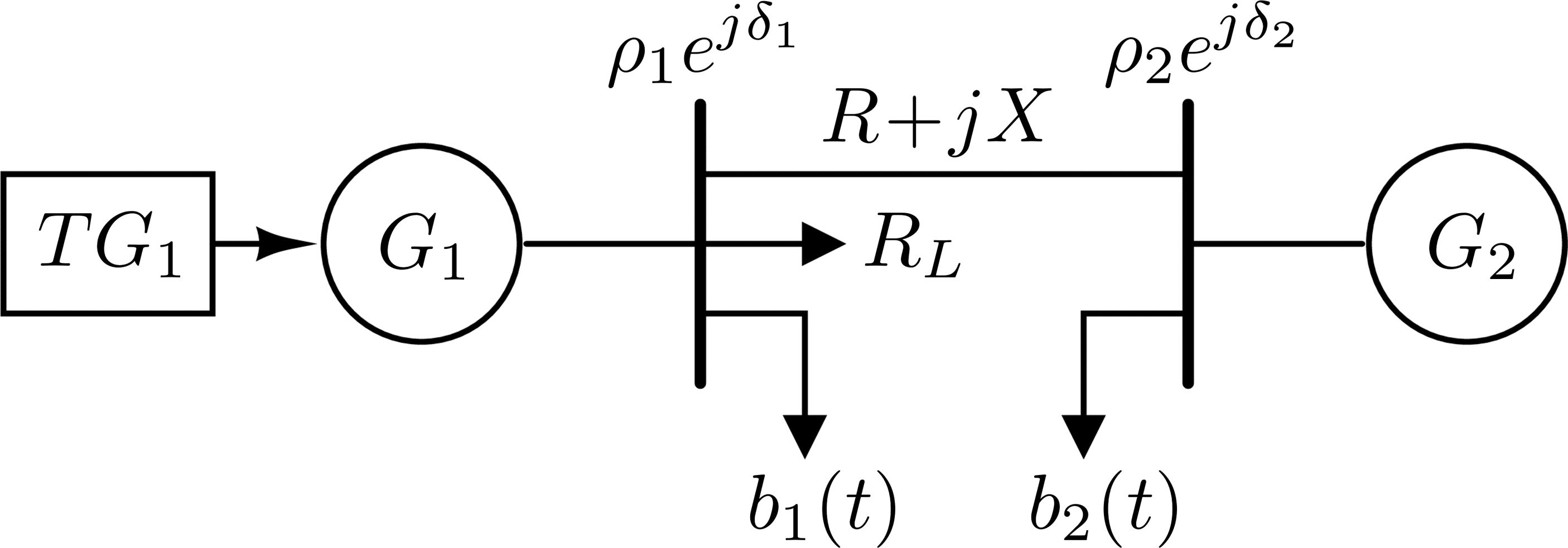
Figure 1: The schematic of the power test system. $\displaystyle R_{L}$ is a resistive load, $\displaystyle b_{1}(t)$ and $\displaystyle b_{2}(t)$ are small-signal (stochastic) perturbations that vary the active power absorbed by the grid at the power flow solution and which are neglected in the large-signal model of the power system. For the sake of simplicity, the internal impedance of both $\displaystyle G_{1}$ and $\displaystyle G_{2}$ is assumed to be zero, and only the $\displaystyle G_{1}$ generator is equipped with a turbine governor.

Our aim is exploiting (14) to systematically derive the $\displaystyle\mathcal{G}_{\mathcal{M}}$ global momentum of a given power system. To give an example-driven insight into the approach we are proposing, we present a simple case-study whose first goal is to show how equation (14) can be derived.

III-A Low-frequency characterization

The large-signal model of the system in Fig. 1, in which the $\displaystyle b_{1}(t)$ and $\displaystyle b_{2}(t)$ small-signals are neglected, is given by the following equations:

$$\begin{array}[]{rcl}\dot{\delta}_{1}&=&\Omega\left(\omega_{1}-\omega_{0}\right)\\ \dot{\delta}_{2}&=&\Omega\left(\omega_{2}-\omega_{0}\right)\\ {\mathcal{M}}_{1}\dot{\omega}_{1}&=&P_{m_{1}}-P_{e_{1}}(\delta_{1},\delta_{2})-{\mathcal{D}}_{1}\left(\omega_{1}-\omega_{0}\right)\\ {\mathcal{M}}_{2}\dot{\omega}_{2}&=&P_{m_{2}}-P_{e_{2}}(\delta_{1},\delta_{2})-{\mathcal{D}}_{2}\left(\omega_{2}-\omega_{0}\right)\\ T_{g_{1}}\dot{P}_{m_{1}}&=&P_{{m_{\mathrm{eq}}}_{1}}-P_{m_{1}}-{k_{g_{1}}}{R_{1}^{-1}}\left(\omega_{1}-\omega_{0}\right)\\ \end{array}~{},$$ (15)

where

$$\begin{array}[]{lcl}P_{e_{1}}(\delta_{1},\delta_{2})&\!\!\!\!\!=\!\!\!\!\!&\frac{1}{R^{2}+X^{2}}\left[R\rho_{1}^{2}-R\rho_{1}\rho_{2}\cos(\delta_{1}-\delta_{2})\right.+\\ &\!\!\!\!\!\!\!\!\!\!&+\left.X\rho_{1}\rho_{2}\sin(\delta_{1}-\delta_{2})\right]+\frac{1}{R_{L}}\rho_{1}^{2}~{},\\ \end{array}$$

and

$$\begin{array}[]{lcl}P_{e_{2}}(\delta_{1},\delta_{2})&\!\!\!\!\!=\!\!\!\!\!&\frac{1}{R^{2}+X^{2}}\left[R\rho_{2}^{2}-R\rho_{1}\rho_{2}\cos(\delta_{2}-\delta_{1})+\right.\\[8.53581pt] &\!\!\!\!\!\!\!\!\!\!&\left.X\rho_{1}\rho_{2}\sin(\delta_{2}-\delta_{1})\right]~{}.\end{array}$$

The last equation in (15) models the turbine governor connected to the $\displaystyle G_{1}$ generator. The power system is assumed to be at steady state, with $\displaystyle{\omega_{k}=\omega_{\mathrm{eq}_{k}}=\omega_{0}=1}$, $\displaystyle{\delta_{k}=\delta_{\mathrm{eq}_{k}}}$, and $\displaystyle{P_{m_{k}}=P_{{m_{\mathrm{eq}}}_{k}}=P_{e_{k}}(\delta_{\mathrm{eq}_{1}},\delta_{\mathrm{eq}_{2}})}$ for $\displaystyle k\in\{1,2\}$. The small signal equivalent model of (15), including now the small-signal additive perturbations projected according to (4), is

$$\begin{array}[]{rcl}\Delta\dot{\delta}_{1}&\!\!\!\!\!=\!\!\!\!\!&\Omega\Delta{\omega_{1}}\\ \Delta\dot{\delta}_{2}&\!\!\!\!\!=\!\!\!\!\!&\Omega\Delta{\omega_{2}}\\ {\mathcal{M}}_{1}\Delta\dot{\omega}_{1}&\!\!\!\!\!=\!\!\!\!\!&\xi(\Delta\delta_{2}-\Delta\delta_{1})-{\mathcal{D}}_{1}\Delta\omega_{1}+\Delta P_{m_{1}}+{\mathcal{M}}_{1}b_{{\delta\omega}_{1}}(t)\\ {\mathcal{M}}_{2}\Delta\dot{\omega}_{2}&\!\!\!\!\!=\!\!\!\!\!&\xi(\Delta\delta_{1}-\Delta\delta_{2})-{\mathcal{D}}_{2}\Delta{\omega_{2}}+{\mathcal{M}}_{2}b_{{\delta\omega}_{2}}(t)\\ T_{g_{1}}\Delta\dot{P}_{m_{1}}&\!\!\!\!\!=\!\!\!\!\!&-\Delta P_{m_{1}}-k_{g_{1}}{R_{1}}^{-1}\Delta\omega_{1}\\ \end{array}$$ (16)

where

$$\xi=\frac{\rho_{1}\rho_{2}}{R^{2}+X^{2}}\left(R\sin(\delta_{\mathrm{eq}_{1}}-\delta_{\mathrm{eq}_{2}})+X\cos(\delta_{\mathrm{eq}_{1}}-\delta_{\mathrm{eq}_{2}})\right)~{}.$$

By transforming equation (16) in the Laplace domain, the $\displaystyle\Delta{\omega_{1}}(s)$ and $\displaystyle\Delta{\omega_{2}}(s)$ small-signal variations of the rotor speeds of the two synchronous generators can be written as

$$\begin{array}[]{l}\displaystyle{\Delta{\omega_{1}}(s)=\frac{\beta_{3}^{1}(s)s^{3}+\beta_{2}^{1}(s)s^{2}+\beta_{1}^{1}(s)s+\beta_{0}^{1}(s)}{\alpha_{4}s^{4}+\alpha_{3}s^{3}+\alpha_{2}s^{2}+\alpha_{1}s+\alpha_{0}}}\\[14.22636pt] \displaystyle{\Delta{\omega_{2}}(s)=\frac{\beta_{3}^{2}(s)s^{3}+\beta_{2}^{2}(s)s^{2}+\beta_{1}^{2}(s)s+\beta_{0}^{2}(s)}{\alpha_{4}s^{4}+\alpha_{3}s^{3}+\alpha_{2}s^{2}+\alpha_{1}s+\alpha_{0}}}\end{array}~{},$$ (17)

where the $\displaystyle\alpha_{k}$ and $\displaystyle\beta_{k}^{j}$ coefficients are reported in Appendix B. For sufficiently small values of $\displaystyle s$ we neglect in (17) the terms $\displaystyle\alpha_{k}s^{k}$ for $\displaystyle k\in\{3,4\}$, and $\displaystyle\beta_{k}^{j}s^{k}$ for $\displaystyle k\in\{2,3\}$ and $\displaystyle j\in\{1,2\}$. Furthermore, in the coefficients reported in Appendix B we neglect all the terms divided by $\displaystyle\xi\Omega$ since we assume $\displaystyle\xi\Omega\gg 1$. Thus we approximate (17) as reported in (18) (next page). The same expression can be straightforwardly derived from the most generic one in (14).

Figure 2 shows the plots corresponding to the expressions in (17) and (18). As it can be noticed, the approximation is extremely good for $\displaystyle f<10\mathrm{Hz}$. The expressions of $\displaystyle\Delta{\omega_{1}}(s)$ and $\displaystyle\Delta{\omega_{2}}(s)$ at low frequencies turn out to be identical; this means that the $\displaystyle\Delta{\delta_{1}}$ and $\displaystyle\Delta{\delta_{2}}$ corresponding angles vary in a synchronized way.

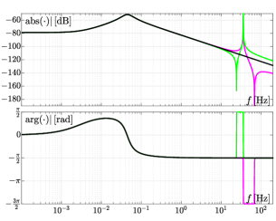
Figure 2: The modulus and the phase of $\displaystyle\Delta\omega_{1}$ (in magenta, see (17)), $\displaystyle\Delta\omega_{2}$ (in green, see (17)), and $\displaystyle\Delta\omega$ (in black, see (18)) are shown in the upper and lower panel, respectively. These curves are derived for the power system in Fig. 1 by assuming $\displaystyle S_{B_{1}}=S_{B_{2}}=100\,\mathrm{M}\mathrm{V}\mathrm{A}$, $\displaystyle D_{1}=D_{2}=1$, $\displaystyle H_{1}=4\,\mathrm{s}$, $\displaystyle H_{2}=2.5\,\mathrm{s}$, $\displaystyle T_{g_{1}}=50\,\mathrm{s}$, $\displaystyle{k_{g_{1}}}{R_{1}^{-1}}=50\,S_{B_{1}}$, $\displaystyle V_{\mathrm{base}}=100\,\mathrm{k}\mathrm{V}$, $\displaystyle Z_{\mathrm{base}}=100\,\mathrm{\SIUnitSymbolOhm}$, $\displaystyle R=X=0.001\,Z_{\mathrm{base}}$, and $\displaystyle R_{L}=\nicefrac{{Z_{\mathrm{base}}}}{{0.9}}$. The power flow solution provides $\displaystyle P_{{m_{\mathrm{eq}}}_{1}}=40\,\mathrm{M}\mathrm{W}$ and $\displaystyle P_{{m_{\mathrm{eq}}}_{2}}=50\,\mathrm{M}\mathrm{W}$. $\displaystyle{\mathcal{M}}_{1}b_{{\delta\omega}_{1}}(t)$ and $\displaystyle{\mathcal{M}}_{2}b_{{\delta\omega}_{2}}(t)$ are sinusoidal functions whose phase is zero and whose amplitude is fixed at $\displaystyle 100\,\mathrm{k}\mathrm{W}$ and $\displaystyle 500\,\mathrm{k}\mathrm{W}$, respectively, for each value of $\displaystyle f$.

$${\Delta{\omega}_{1}(s)\simeq\Delta{\omega}_{2}(s)\simeq\Delta{\omega}(s)\equiv\frac{(sT_{g_{1}}+1)({\mathcal{M}}_{1}b^{\mathrm{lf}}_{{\delta\omega}_{1}}(s)+{\mathcal{M}}_{2}b^{\mathrm{lf}}_{{\delta\omega}_{2}}(s))}{s^{2}\left({\mathcal{M}}_{1}+{\mathcal{M}}_{2}\right)T_{g_{1}}+s\left(({\mathcal{D}}_{1}+{\mathcal{D}}_{2})T_{g_{1}}+{\mathcal{M}}_{1}+{\mathcal{M}}_{2}\right)+\left(\left({\mathcal{D}}_{1}+{\mathcal{D}}_{2}\right)+{k_{g_{1}}R_{1}^{-1}}\right)}}$$ (18)

III-B Global momentum estimation

Equation (18) can be recast as

$$\begin{array}[]{l c l}\Delta\omega_{1}(s)&=&\left(\frac{c_{1}}{s-a_{1}}+\frac{c_{2}}{s-a_{2}}\right)\eta(s)\\[14.22636pt] &=&\frac{(c_{1}+c_{2})s-c_{1}a_{2}-c_{2}a_{1}}{s^{2}-s(a_{1}+a_{2})+a_{1}a_{2}}\eta(s)\\[14.22636pt] &=&\frac{\left(\frac{1}{{\mathcal{M}}_{1}+{\mathcal{M}}_{2}}s+\frac{1}{({\mathcal{M}}_{1}+{\mathcal{M}}_{2})T_{g1}}\right)\eta(s)}{s^{2}+\left(\frac{1}{T_{g1}}+\frac{{\mathcal{D}}_{1}+{\mathcal{D}}_{2}}{{\mathcal{M}}_{1}+{\mathcal{M}}_{2}}\right)s+\frac{{\mathcal{D}}_{1}+{\mathcal{D}}_{2}+{k_{g_{1}}R_{1}^{-1}}}{({\mathcal{M}}_{1}+{\mathcal{M}}_{2})T_{g1}}}\end{array}$$ (19)

where $\displaystyle a_{1}$ and $\displaystyle a_{2}$ are the poles, $\displaystyle c_{1}$ and $\displaystyle c_{2}$ are the residues, and $\displaystyle\eta(s)={\mathcal{M}}_{1}b^{\mathrm{lf}}_{{\delta\omega}_{1}}(s)+{\mathcal{M}}_{2}b^{\mathrm{lf}}_{{\delta\omega}_{2}}(s)$.

From (19) we see that $\displaystyle\mathcal{G}_{M}={\mathcal{M}}_{1}+{\mathcal{M}}_{2}$ can be derived through the $\displaystyle c_{1}+c_{2}$ term by performing an experiment. Let us assume to vary $\displaystyle{\mathcal{M}}_{1}$ of a known constant value $\displaystyle\Delta{\mathcal{M}}$ (varying $\displaystyle{\mathcal{M}}_{2}$ is totally equivalent). This variation does not alter the power flow solution of the system but how the $\displaystyle G_{1}$ generator reacts to variations of its rotor speed. Before the experiment, we have $\displaystyle c_{1}+c_{2}=({\mathcal{M}}_{1}+{\mathcal{M}}_{2})^{-1}$ and after the experiment $\displaystyle\widehat{c}_{1}+\widehat{c}_{2}=({\mathcal{M}}_{1}+{\mathcal{M}}_{2}+\Delta{\mathcal{M}})^{-1}$ from which we derive

$$\mathcal{G}_{M}=\frac{\widehat{c}_{1}+\widehat{c}_{2}}{c_{1}+c_{2}-\widehat{c}_{1}-\widehat{c}_{2}}\Delta{\mathcal{M}}~{}.$$ (20)

At first we perform a proper frequency scan of the system by acting on either $\displaystyle b_{1}(t)$ or $\displaystyle b_{2}(t)$ (or both) to numerically derive (18). Then, we use the vf technique [19, 20, 21] to fit (19) and determine the pairs of $\displaystyle c_{1}$, $\displaystyle c_{2}$ and $\displaystyle\widehat{c}_{1}$ and $\displaystyle\widehat{c}_{2}$ coefficients (i.e., before and after the experiment) and, thus, $\displaystyle\mathcal{G}_{M}$.

This approach presents several drawbacks. First and foremost, in practice it is typically not possible to act on the inertia constant of the synchronous machines. Secondly, a complete frequency scan is also unfeasible. Lastly, the rotor speed of the synchronous machines is unlikely to be available. In the following we show how to overcome these issues.

IV A method for the estimation of the power-system global momentum

The experiment described in Sec. III-B can be implemented by resorting to a grid-forming (gf) converter-interfaced generator (cig). This device may already be present in the power system or alternatively can be inserted with the specific purpose of allowing the estimation of the power system global momentum. As shown in Sec. V, the state equations governing the dynamics of this device are similar to those reported in (1). Hence its equivalent rotor speed $\displaystyle{\omega}_{\mathrm{gf}}$ becomes one of the entries of the $\displaystyle\boldsymbol{\omega}$ vector and its equivalent momentum constant one of the diagonal elements of the $\displaystyle\boldsymbol{{\mathcal{M}}}$ matrix. Proper low-frequency small-signal tones injected through the gf cig itself may contribute to the $\displaystyle\boldsymbol{\mathbbm{1}}_{1,N}\boldsymbol{{\mathcal{M}}}\boldsymbol{b}_{\delta\omega}(s)$ term in equation (14). By observing the frequency response of the equivalent rotor speed of the gf cig, once those tones are injected, we can obtain a proper set of samples of (14). We recall that (14) provides the expression in the Laplace domain shared (at low frequency) by all the components of $\displaystyle\boldsymbol{\omega}$ and hence of $\displaystyle{\omega}_{\mathrm{gf}}$. By varying the gf cig equivalent momentum constant and fitting the samples of (14) before and after this variation, it is possible to derive the global momentum of the entire power system.

We underline that the reader must not be confused at this point: by injecting small-signal power perturbations in the cig and measuring its virtual rotor speed, we do not estimate the cig virtual contribution to the overall system momentum, as it is done in several papers in the literature. On the contrary, we estimate the global momentum of the entire power system (cig included). In other words, the cig can be viewed as a probing-signal source, whose virtual inertia is known and can be modified during the experiment needed to obtain $\displaystyle\mathcal{G}_{M}$.

The method we developed gives a continuous estimate of the global momentum. Since we use the vf algorithm [19, 20, 21] to estimate the residues and the poles of (14), we need frequency samples of both its modulus and phase. This forbids resorting to the power spectral density of $\displaystyle{\omega}_{\mathrm{gf}}$ when its fluctuation is solely given by the noisy generated/absorbed powers. We thus opted to modulate the power injected by the cig by a discrete set of $\displaystyle\mathcal{N}_{\mathcal{T}}$ deterministic and coherent small-signal sinusoidal tones $\displaystyle s_{w}(t)$ ($\displaystyle w=1,\dots,\mathcal{N}_{\mathcal{T}}$). The choices of $\displaystyle\mathcal{N}_{\mathcal{T}}$ and of the $\displaystyle f_{w}$ frequency of each tone depend on the bandwidth that has to be explored to fit (14). It is worth mentioning that $\displaystyle\mathcal{N}_{\mathcal{T}}$ must be fixed in excess with respect to the residues and poles number of (14). Injection of small-signal tones in a power system is not an unusual technique and it was already adopted in [33, 9]. A good description of this technique is in [3]. The $\displaystyle s_{w}(t)$ tones are very slowly varying and of modest magnitude, therefore they do not impact the stability of the power system.

The equivalent inertia constant of the cig varies as a square waveform of amplitude $\displaystyle\Delta{\mathcal{M}}$, period $\displaystyle T_{\Delta{\mathcal{M}}}$, and duty cycle $\displaystyle 50\%$. The power system is stimulated by injecting the $\displaystyle s_{w}(t)$ waveforms and the time samples of $\displaystyle{\omega}_{\mathrm{gf}}$ are collected. We computed the $\displaystyle\gamma_{w_{c}}$ and $\displaystyle\gamma_{w_{s}}$ direct and quadrature components of the Fourier integrals of $\displaystyle{\omega}_{\mathrm{gf}}$ at each $\displaystyle f_{q}$ frequency as

$$\begin{array}[]{l}\displaystyle{\gamma_{w_{c}}=\mu f_{w}\int_{t_{0}}^{t_{0}+\frac{\mu}{f_{w}}}{{\omega}_{\mathrm{gf}}(t)\cos(2\pi\mu f_{w}t)dt}}\\[11.38109pt] \displaystyle{\gamma_{w_{s}}=\mu f_{w}\int_{t_{0}}^{t_{0}+\frac{\mu}{f_{w}}}{{\omega}_{\mathrm{gf}}(t)\sin(2\pi\mu f_{w}t)dt}}~{}.\end{array}$$ (21)

The $\displaystyle\gamma_{w_{c}}$ and $\displaystyle\gamma_{w_{s}}$ terms constitute the frequency samples that feed the vf algorithm. Note that if it is necessary to reduce the effects of noise to increase the signal-to-noise ratio, the integrals in (21) can be computed over a time interval $\displaystyle\nicefrac{{\mu}}{{f_{w}}}$ which is a multiple of the period of the corresponding tone $\displaystyle s_{w}(t)$. The $\displaystyle t_{0}$ time instant in (21) coincides with the rising and falling edges of the square waveform used to periodically change the virtual inertia of the cig. Assuming $\displaystyle s_{1}(t)$ as the tone with the lowest frequency, $\displaystyle f_{1}$ suggests how to choose $\displaystyle T_{\Delta{\mathcal{M}}}$, i.e., $\displaystyle\nicefrac{{T_{\Delta{\mathcal{M}}}}}{{2}}>\nicefrac{{\mu}}{{f_{1}}}$.

As shown in the next section, the proposed estimation method can be applied to bigger power systems than that shown in Fig. 1 by resorting to (14). Indeed, also (14) can be recast through a partial fraction decomposition analogous to (19). Thus, even in more complex cases, the process to estimate the global momentum of inertia still relies on (20) and vector fitting.

V Numerical examples

V-A Virtual synchronous generator

A grid-forming (gf) converter-interfaced generator (cig) implements a control scheme that simulates the mechanical dynamical behavior of a synchronous machine (swing equation) by means of a power converter. The goal is to provide inertia, damping, primary frequency control, and voltage control to a network with a significant penetration of renewable energy sources and therefore reduced inertia.

The proposed approach to estimate the $\displaystyle\mathcal{G}_{M}$ global momentum exploits the cig model described in [18]. It provides virtual inertia by implementing the swing equation with frequency droop control and replicates the stator impedance of the synchronous generator. Importantly, the vast majority of cigs that provide synthetic inertia reproduce exclusively the mechanical behavior of a synchronous machine (i.e., the swing equation), while failing to replicate its full electro-mechanical behavior due to windings, including dampers. On the other hand, they add the dynamics of the electronic converter. The cig model in [18] belongs to this category and therefore implements only the swing equation, leading to a different spectral footprint at high frequencies with respect to a real synchronous generator. The swing equation implemented in [18] is

$$\begin{array}[]{rcl}\dot{\delta}_{\mathrm{gf}}&=&\Omega\left(\omega_{\mathrm{gf}}-\omega_{0}\right)\\[2.84526pt] T_{a}\dot{\omega}_{\mathrm{gf}}&=&\left(1+\eta_{\mathrm{gf}}\right)P_{g}-P_{e}-K_{d}\left(\omega_{\mathrm{pll}}-\omega_{\mathrm{gf}}\right)+\\ &&-K_{w}\left(\omega_{\mathrm{gf}}-\omega_{\mathrm{0}}\right)\\[2.84526pt] P_{e}&=&\frac{V_{d}I_{d}+V_{q}I_{q}}{P_{\mathrm{ref}}}\end{array}~{},$$

where $\displaystyle V_{d}$, $\displaystyle I_{d}$, $\displaystyle V_{q}$, and $\displaystyle I_{q}$ are the voltages and currents of the generator in the dq-frame that lead to the $\displaystyle P_{e}$ electrical active power (per-unit), $\displaystyle P_{\mathrm{ref}}$ is the power rating of the cig, $\displaystyle T_{a}$ is the (virtual) inertia constant, $\displaystyle P_{g}$ is the generated power setpoint at system frequency $\displaystyle\omega_{0}$ (per-unit), $\displaystyle K_{w}$ is the load-damping, $\displaystyle\delta_{\mathrm{gf}}$ if the angle deviation of the virtual rotor, $\displaystyle\omega_{\mathrm{gf}}$ is the virtual rotor angular speed (per-unit), $\displaystyle\omega_{\mathrm{pll}}$ is the electrical angular frequency of the voltage at the connection bus (per-unit), $\displaystyle K_{d}$ regulates the virtual rotor speed according to the electrical angular frequency of the bus to which the cig is connected, thus emulating frequency slip (in our case $\displaystyle K_{d}=0$). $\displaystyle\eta_{\mathrm{gf}}$ is the small signal used to perturb the power system, which modulates the active power setpoint of the cig.

V-B Load models

The loads that are present in the power systems considered here as case studies allow to perturb their active power. The $\displaystyle l-$th of these loads (for $\displaystyle l=1,\dots,L$) is modeled as

$$\mathrm{L}_{l}=\left(1+\eta_{l}(t)\right)\,P_{{\mathrm{L0}}_{l}}\left(\frac{\left|V_{l}\right|}{V_{0_{l}}}\right)^{\gamma}~{},$$ (22)

where $\displaystyle P_{{\mathrm{L0}}_{l}}$ is the nominal active power of the load, $\displaystyle V_{0_{l}}$ is the load voltage rating, $\displaystyle V_{l}$ is the bus voltage at which the load is connected, and $\displaystyle\gamma$ governs the dependence of the load on bus voltage (hereafter assumed to be null). By applying the $\displaystyle\eta_{l}(t)$ small signal we can perturb the load power.

In the time domain simulations of stochastic load fluctuations, we assume that $\displaystyle\eta_{l}(t)$ is an Ornstein-Uhlenbeck (ou) process [29]. The ou processes (one for each load) are defined through the set of stochastic differential equations

$$d\boldsymbol{\eta}=-\boldsymbol{\Upsilon}\boldsymbol{\eta}\,dt+\boldsymbol{\Sigma}\,d\boldsymbol{W}_{t}~{},$$ (23)

where the drift $\displaystyle{\boldsymbol{\Upsilon}\in\mathbb{R}^{L\times L}}$ and diffusion $\displaystyle{\boldsymbol{\Sigma}\in\mathbb{R}^{L\times L}}$ are diagonal matrices with positive entries, $\displaystyle\boldsymbol{W}_{t}\in\mathbb{R}^{L}$ is a vector of Wiener processes, and the differentials rather than time derivatives are utilized to account for the idiosyncrasies of sdes. The ou processes are characterized by a mean-reversion property and exhibit bounded standard deviation. Moreover, these processes show a spectrum that is an accurate model of the stochastic variability of power loads [34, 35, 29, 31, 36].

To carry out the simulations discussed below, the numerical integration of the multi-dimensional ou process in (23) was based on the numerical scheme proposed by Gillespie in [37]. Furthermore, the second-order trapezoidal implicit weak scheme for stochastic differential equations with colored noise, available in the simulator pan [38, 39, 40], was adopted [41].

V-C The ieee 39-bus test system

We used as first benchmark the ieee 39-bus system [42]. The grid contains $\displaystyle 10$ generators and $\displaystyle 46$ lines and it is a simplified model of the New England power system. Its schematic is reported in Fig. 3.

Figure 3: Schematic of the ieee 39-bus system.

The $\displaystyle G_{1}$ generator models the aggregate behavior of a large number of generators. This is reflected in its momentum value ($\displaystyle\mathcal{M}_{G_{1}}=100\,\mathrm{G}\mathrm{J}$), which is one order of magnitude larger than that of the other generators in the network (see Table I).

TABLE I: Synchronous generators $\displaystyle H$ and $\displaystyle S_{B}$

Gen.	$\displaystyle H\,[\mathrm{s}]$	$\displaystyle S_{B}\,[\mathrm{M}\mathrm{W}]$	Gen.	$\displaystyle H\,[\mathrm{s}]$	$\displaystyle S_{B}\,[\mathrm{M}\mathrm{W}]$
$\displaystyle G_{1}$	$\displaystyle 5.00$	$\displaystyle 10000$	$\displaystyle G_{6}$	$\displaystyle 4.35$	$\displaystyle 800$
$\displaystyle G_{2}$	$\displaystyle 4.33$	$\displaystyle 700$	$\displaystyle G_{7}$	$\displaystyle 3.77$	$\displaystyle 700$
$\displaystyle G_{3}$	$\displaystyle 4.47$	$\displaystyle 800$	$\displaystyle G_{8}$	$\displaystyle 3.47$	$\displaystyle 700$
$\displaystyle G_{4}$	$\displaystyle 3.57$	$\displaystyle 800$	$\displaystyle G_{9}$	$\displaystyle 3.45$	$\displaystyle 1000$
$\displaystyle G_{5}$	$\displaystyle 4.33$	$\displaystyle 600$	$\displaystyle G_{10}$	$\displaystyle 4.20$	$\displaystyle 1000$

The ieee 39-bus system version we started from is that in the distribution of powerfactory by digsilent.

The cig, used to generate the perturbing power tones and to perform the experiment in the proposed global momentum estimation, is connected at bus14. There is not a preferred bus to which the cig should be connected. We inserted two additional cigs at bus8 and bus27 to show that the proposed estimation algorithm takes into account every component affecting the global momentum. The former models an aggregated wind power plant and the latter a battery storage system. Each cig is characterized by a $\displaystyle 5\,\mathrm{G}\mathrm{J}$ momentum.

Firstly, we performed an (ideal) frequency scan assuming $\displaystyle\eta_{\mathrm{gf}}(t)$ as a small-signal sinusoidal source and by turning off the stochastic variations of the loads. So doing, we computed all the transfer functions between $\displaystyle\eta_{\mathrm{gf}}(t)$ and the rotor speed of each synchronous machine and cig. Figure 4 (upper panel) reports these transfer functions.

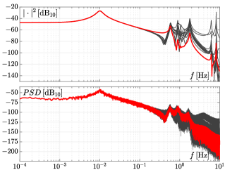
Figure 4: Upper panel: the magnitude squared of the transfer functions between $\displaystyle\eta_{\mathrm{gf}}(t)$ and the rotor speed of each synchronous machine and cig of the (modified) ieee 39-bus system. Lower panel: power spectral densities of the rotor speed of each synchronous machine and cig of the (modified) ieee 39-bus system when the stochastic noise in the loads is turned on. In both the panels the red curve refers to the cig connected at bus14.

We can notice that they almost perfectly overlap at frequencies below $\displaystyle 0.1\,\mathrm{Hz}$ while they sensibly differ for higher frequency values. This result carries similar information as that in Fig. 2. Note that these transfer functions show how rotor speeds deviate from $\displaystyle\omega_{0}$ under the assumption of small signal behavior (linear behavior in the neighborhood of the equilibrium point, i.e., power-flow). These spectra show that if we think of a step perturbation, during the first time interval after its application, say $\displaystyle{100\,\mathrm{m}\mathrm{s}\rightarrow 10\,\mathrm{Hz}}$, the synchronous generators lose synchrony and counteract power imbalance in a non-coordinated way. This behavior persists up to $\displaystyle 2\,\mathrm{s}\rightarrow 0.5\,\mathrm{Hz}$, at which point the synchronous generators and cigs go toward re-synchronization (low frequency behavior). By observing the low frequency overlapping of all the curves in Fig. 4, the global momentum can be determined through (14) by fitting only the curve related to the cig connected at bus14 in the $\displaystyle[6,30]\,\mathrm{m}\mathrm{Hz}$ frequency interval, since all rotor speeds are described by the same behavior in this frequency interval (principal frequency system dynamics), as predicted by our analysis. The frequency behavior in this band is exclusively due to the mechanical characteristics of the power system contributed by synchronous generators and prime movers (swing equation) and by cigs that implement virtual inertia contribution.

We exploited this frequency scan to estimate the global momentum of the ieee 39-bus system. We performed 500 independent frequency scans and for each of those the inertia constant of each generator was uniformly randomly varied by $\displaystyle\pm 30\%$ with respect to its nominal value. This was done to test the method on a large set of inertia configurations. At each run, we used the vf method to fit the frequency behavior of the cig virtual rotor angular frequency before and after the experiment and estimated the global momentum. The left violin plot in Fig. 5(a) summarizes the performance of the proposed approach, in terms of the $\displaystyle\epsilon_{\%}$ percent relative error, in estimating the global momentum for each one of the $\displaystyle 500$ random configurations.

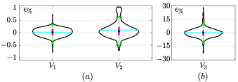
Figure 5: The horizontal cyan segments and the black solid circle markers correspond to the mean $\displaystyle\mu$ and the median $\displaystyle\mu_{\text{dn}}$ of the results, respectively. The magenta bars represent the iqr, viz. the spread difference between the $\displaystyle 75^{\mathrm{th}}$ and $\displaystyle 25^{\mathrm{th}}$ percentiles of the data. The green solid circle markers represent the upper adjacent value (i.e., the largest observation that is less than or equal to the third quartile plus $\displaystyle 1.5\times\acs{iqr}$) and the lower adjacent value (i.e., the smallest observation that is greater than or equal to the first quartile minus $\displaystyle 1.5\times\acs{iqr}$). Panel (a). The $\displaystyle V_{1}$ violin plot ($\displaystyle\mu=0.019$, $\displaystyle\mu_{\text{dn}}=0.026$, and $\displaystyle\acs{iqr}=0.232$) refers to the results obtained by exploiting an ideal frequency scan assuming $\displaystyle\eta_{\mathrm{gf}}(t)$ as a small-signal sinusoidal source. The simulations were carried out in the frequency-domain by resorting to the AC analysis. The $\displaystyle V_{2}$ violin plot ($\displaystyle\mu=0.105$, $\displaystyle\mu_{\text{dn}}=0.062$, and $\displaystyle\acs{iqr}=0.302$) refers to the results obtained by injecting a set of $\displaystyle\mathcal{N}_{\mathcal{T}}=10$ deterministic and coherent small signal sinusoidal tones through the cig connected at bus14. The simulations were carried out in the time-domain and the integrals in equation (21) were computed to feed the vf algorithm. Both $\displaystyle V_{1}$ and $\displaystyle V_{2}$ were obtained by assuming that all the loads as noiseless. Panel (b). Contrary to $\displaystyle V_{2}$, the $\displaystyle V_{3}$ violin plot ($\displaystyle\mu=0.074$, $\displaystyle\mu_{\text{dn}}=-0.104$, and $\displaystyle\acs{iqr}=5.48$) was derived by turning on the stochastic noise in the loads.

Since as said before, this ideal frequency scan is not practical, we turned on the injection of the discrete set of $\displaystyle\mathcal{N}_{\mathcal{T}}=10$ deterministic and coherent small signal sinusoidal tones by the cig connected at bus14. We performed $\displaystyle 500$ time domain simulations lasting $\displaystyle 15\,\mathrm{min}$ and we randomly varied the inertia configuration. Before varying the inertia configuration as detailed in Section IV we performed the “experiment” and computed the global momentum. The information of the $\displaystyle\epsilon_{\%}$ percent relative error in estimating the global momentum are shown by the right violin plot in Fig. 5(a). We can notice that the overall performance is worsened even if it remains very good since the relative accuracy in determining the global momentum is in any case lower than $\displaystyle 2.0\%$.

Finally we turned on the stochastic noise in the loads. In the lower panel of Fig. 4, we report the frequency behavior of the rotor speed of all the synchronous machines and cigs when all the loads of the network are perturbed as described in Sec. V-B. We used $\displaystyle L=19$ independent $\displaystyle\eta_{z}$ small-signal stochastic noise sources, one for each power load. We choose a $\displaystyle 2\,\mathrm{s}$ reversion time and set $\displaystyle\sigma_{z}$ (see (23)) in such a way that the standard deviation of $\displaystyle\eta_{l}(t)$ is $\displaystyle 0.5\%$ of $\displaystyle P_{L0_{l}}$ (nominal load active power) in (22). The zero mean implies that the stochastic loads power fluctuations do not perturb, on average, the operating point of the system. By observing the spectral densities in Fig. 4 (lower panel), we notice a different behavior of the rotor speed deviations at frequency above $\displaystyle 0.1\,\mathrm{Hz}$ but once more spectra almost perfectly overlap at lower frequencies. This means that the effect of the stochastic noise sources will be superimposed to that of the $\displaystyle\mathcal{N}_{\mathrm{T}}$ tones injected by the cig.

We ran $\displaystyle 500$ time-domain large-signal simulations with the nominal momentum configuration and with a magnitude of the injected tones that cause a peak power variation less than $\displaystyle 2.5\%$ of the nominal power of the ieee 39-bus system. The violin plot giving information about the relative error in the global momentum estimation is shown in Fig. 5(b).

We see that the relative error is further increased with respect to the previous cases. This is due to the decreased signal-to-noise-ratio (snr) that makes more difficult the fitting of equation (14) by the vf method.

V-D The ieee118 power system

As a second benchmark we used the ieee 118-bus system. It represents an approximation of the American Electric Power system (in the U.S. Midwest) as of December 1962. It contains $\displaystyle 19$ generators, $\displaystyle 35$ synchronous condensers, $\displaystyle 177$ lines, $\displaystyle 9$ transformers, and $\displaystyle 91$ loads. The original model is available in the distribution of matpower [43], but it does not contain any dynamic model. There are several versions enhanced with dynamic models; guiding rules can be found in [44].

The gf cig, used to generate the perturbing power tones and to perform the experiment, is connected at bus38. As already said for the ieee 39-bus there is not a preferred bus to which the cig should be connected.

The result by the (ideal) frequency scan assuming $\displaystyle\eta_{\mathrm{gf}}(t)$ as a small-signal sinusoidal source is shown in Fig. 6. We see that as for the ieee 39-bus system all the angular frequencies of synchronous machine rotors and cig overlap almost perfectly at low frequency ($\displaystyle<100\,\mathrm{m}\mathrm{Hz}$).

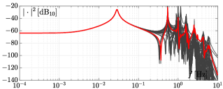
Figure 6: The magnitude squared of the transfer functions between $\displaystyle\eta_{\mathrm{gf}}(t)$ injected through the gf cig connected at bus101 and the rotor speed of each synchronous machine and cig of the (modified) ieee 118-bus system. The red curve refers to the (virtual) rotor speed of the cig connected at bus101.

We thus repeated the same simulation we had done with the ieee39, that is, the inertia of each generator was uniformly randomly varied of $\displaystyle\pm 30\%$ with respect to its nominal value and we estimated the global inertia by a frequency scan in the time domain with noiseless loads and finally with noisy loads. The results are summarized by the violin plots in Fig. 7 and have the same meaning of those in Fig. 5.

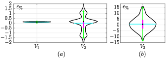
Figure 7: Panel (a). The $\displaystyle V_{1}$ violin plot: $\displaystyle\mu=0.115$, $\displaystyle\mu_{\text{dn}}=0.117$, and $\displaystyle\acs{iqr}=0.055$. The $\displaystyle V_{2}$ violin plot: $\displaystyle\mu=-0.002$, $\displaystyle\mu_{\text{dn}}=0.170$, and $\displaystyle\acs{iqr}=0.680$. Panel (b). The $\displaystyle V_{3}$ violin plot: $\displaystyle\mu=0.675$, $\displaystyle\mu_{\text{dn}}=0.592$, and $\displaystyle\acs{iqr}=7.01$. The simulation setup for the $\displaystyle V_{k}$ violin plot ($\displaystyle k\in\{1,2,3\}$) is the same one of the $\displaystyle k-$th plot in Fig. 5.

We see that very good estimation results of global momentum are obtained also for the ieee 118-bus system.

VI Concluding remarks

We propose a method to estimate the global momentum of electrical power systems that requires only measured data from a grid-forming (gf) converter-interfaced generator (cig) that is already present in the system or that can be added for this purpose.

The approach is fully data-driven and proved accurate even in complex systems and can take into account both conventional and virtual synchronous machines.

Estimations of global momentum of the ieee 39-bus and larger ieee 118-bus test systems lead to an average percent relative error lower than $\displaystyle 1\%$ (with an interquartile range lower than $\displaystyle 7\%$), when the inertia of each generator is varied in a uniformly random fashion by $\displaystyle\pm 30\%$ and noise by loads is considered. The estimation algorithm runs in less than $\displaystyle 10\,\mathrm{s}$ on a conventional computer.

We believe that the proposed technique can be useful to monitor the total frequency support provided by conventional and virtual-synchronous devices. In the near future we plan to explore other extrapolation procedures that allow the use of noise by stochastic load/generation and to use this technique on real data measured by pmu.

Appendix A

To derive the $\displaystyle\boldsymbol{v}_{1}$ left-eigenvector reported in (5) we write

$$\boldsymbol{A}^{\mathrm{T}}=\left[\!\!\!\!\begin{array}[]{c c c}\boldsymbol{\mathbbm{O}}_{N}&-\boldsymbol{\Pi}\boldsymbol{{\mathcal{M}}}^{-1}&\boldsymbol{\mathbbm{O}}_{N}\\ \Omega\boldsymbol{\mathbbm{1}}_{N}&\boldsymbol{{\mathcal{M}}}^{-1}\boldsymbol{{\mathcal{D}}}&-\boldsymbol{T}^{-1}_{g}\boldsymbol{k}_{g}\boldsymbol{R}^{-1}\\ \boldsymbol{\mathbbm{O}}_{N}&\boldsymbol{{\mathcal{M}}}^{-1}&-\boldsymbol{T}^{-1}_{g}\\ \end{array}\!\!\!\!\right]$$ (24)

and we have to solve $\displaystyle\boldsymbol{A}^{\mathrm{T}}\boldsymbol{v}_{1}=\boldsymbol{\mathbbm{O}}_{3N,1}$. By choosing $\displaystyle\boldsymbol{v}_{1}=(\boldsymbol{v}_{\delta}^{\mathrm{T}},\boldsymbol{v}_{\omega}^{\mathrm{T}},\boldsymbol{v}_{P_{m}}^{\mathrm{T}})^{\mathrm{T}}$, this implies

$$\left\{\begin{array}[]{l}\boldsymbol{\Pi}\boldsymbol{{\mathcal{M}}}^{-1}\boldsymbol{v}_{\omega}=\boldsymbol{\mathbbm{O}}_{N,1}\\ \Omega\boldsymbol{v}_{\delta}+\boldsymbol{{\mathcal{M}}}^{-1}\boldsymbol{{\mathcal{D}}}\boldsymbol{v}_{\omega}-\boldsymbol{T}^{-1}_{g}\boldsymbol{k}_{g}\boldsymbol{R}^{-1}\boldsymbol{v}_{P_{m}}=\boldsymbol{\mathbbm{O}}_{N,1}\\ \boldsymbol{{\mathcal{M}}}^{-1}\boldsymbol{v}_{\omega}-\boldsymbol{T}^{-1}_{g}\boldsymbol{v}_{P_{m}}=\boldsymbol{\mathbbm{O}}_{N,1}\\ \end{array}\ \right.~{}.$$

From the first equation above, being $\displaystyle\ker(\boldsymbol{\Pi})=\boldsymbol{\mathbbm{1}}_{N,1}$, we find $\displaystyle\boldsymbol{v}_{\omega}=\boldsymbol{{\mathcal{M}}}\boldsymbol{\mathbbm{1}}_{N,1}$. Hence, from the third equation, $\displaystyle\boldsymbol{v}_{P_{m}}=\boldsymbol{T}_{g}\mathbbm{1}_{N,1}$, and, from the second one, $\displaystyle\boldsymbol{v}_{\delta}=\Omega^{-1}(\boldsymbol{{\mathcal{D}}}+\boldsymbol{k}_{g}\boldsymbol{R}_{g}^{-1})\boldsymbol{\mathbbm{1}}_{N,1}$. Since $\displaystyle\boldsymbol{u}_{1}=[\boldsymbol{\mathbbm{1}}_{1,N},\boldsymbol{\mathbbm{O}}_{1,2N}]^{\mathrm{T}}$, then

$$\boldsymbol{v}_{1}^{\mathrm{T}}\boldsymbol{u}_{1}=\Omega^{-1}\mathbbm{1}_{1,N}\left(\boldsymbol{{\mathcal{D}}}+\boldsymbol{k}_{g}\boldsymbol{R}_{g}^{-1}\right)\boldsymbol{\mathbbm{1}}_{N,1}~{},$$

and it is possible to normalize $\displaystyle\boldsymbol{v}_{1}^{\mathrm{T}}$ in such a way that $\displaystyle\boldsymbol{v}_{1}^{\mathrm{T}}\boldsymbol{u}_{1}=1$ thus obtaining equation (5).

Appendix B

$$\displaystyle\beta_{3}^{1}(s)= \displaystyle{\mathcal{M}}_{1}{\mathcal{M}}_{2}R_{1}T_{g_{1}}b_{{\delta\omega}_{1}}(s)$$

$$\displaystyle\beta_{2}^{1}(s)= \displaystyle{\mathcal{M}}_{1}\left({\mathcal{D}}_{2}T_{g_{1}}+{\mathcal{M}}_{2}\right)R_{1}b_{{\delta\omega}_{1}}(s)$$

$$\displaystyle\beta_{1}^{1}(s)= \displaystyle\left(\rule{0.0pt}{13.37277pt}(b_{{\delta\omega}_{1}}(s){\mathcal{M}}_{1}+b_{{\delta\omega}_{2}}(s){\mathcal{M}}_{2})T_{g_{1}}+\frac{}{}\right.$$

$$\displaystyle+\left.\frac{b_{{\delta\omega}_{1}}(s){\mathcal{M}}_{1}{\mathcal{D}}_{2}}{\xi\Omega}\right)\xi\Omega R_{1}$$

$$\displaystyle\beta_{0}^{1}(s)= \displaystyle\left(b_{{\delta\omega}_{1}}(s){\mathcal{M}}_{1}+b_{{\delta\omega}_{2}}(s){\mathcal{M}}_{2}\right)\xi\Omega R_{1}$$

$$\displaystyle\beta_{3}^{2}(s)= \displaystyle{\mathcal{M}}_{1}{\mathcal{M}}_{2}R_{1}T_{g_{1}}b_{{\delta\omega}_{2}}(s)$$

$$\displaystyle\beta_{2}^{2}(s)= \displaystyle{\mathcal{M}}_{2}\left({\mathcal{D}}_{1}T_{g_{1}}+{\mathcal{M}}_{1}\right)R_{1}b_{{\delta\omega}_{2}}(s)$$

$$\displaystyle\beta_{1}^{2}(s)= \displaystyle\left(\rule{0.0pt}{12.51918pt}(b_{{\delta\omega}_{1}}(s){\mathcal{M}}_{1}+b_{{\delta\omega}_{2}}(s){\mathcal{M}}_{2})T_{g_{1}}+\frac{}{}\right.$$

$$\displaystyle+\left.\frac{b_{{\delta\omega}_{2}}(s){\mathcal{M}}_{2}({\mathcal{D}}_{1}+k_{g_{1}}R_{1}^{-1})}{\xi\Omega}\right)\xi\Omega R_{1}$$

$$\displaystyle\beta_{0}^{2}(s)= \displaystyle\beta_{0}^{1}(s)$$

$$\displaystyle\alpha_{4}= \displaystyle{\mathcal{M}}_{1}{\mathcal{M}}_{2}R_{1}T_{g_{1}}$$

$$\displaystyle\alpha_{3}= \displaystyle R_{1}(T_{g_{1}}(D_{2}M_{1}+D_{1}M_{2})+M_{1}M_{2})$$

$$\displaystyle\alpha_{2}= \displaystyle\left(\frac{{\mathcal{D}}_{2}\left({\mathcal{D}}_{1}T_{g_{1}}+{\mathcal{M}}_{1}\right)+{\mathcal{D}}_{1}{\mathcal{M}}_{2}}{\xi\Omega}+\frac{}{}\right.$$

$$\displaystyle\left.+\left({\mathcal{M}}_{1}+{\mathcal{M}}_{2}\right)T_{g_{1}}+\frac{k_{1}R_{1}^{-1}{\mathcal{M}}_{2}}{\xi\Omega}\right)\xi\Omega R_{1}$$

$$\displaystyle\alpha_{1}= \displaystyle\left(\rule{0.0pt}{17.07164pt}({\mathcal{D}}_{1}+{\mathcal{D}}_{2})T_{g_{1}}+{\mathcal{M}}_{1}+{\mathcal{M}}_{2}+\frac{}{}\right.$$

$$\displaystyle+\left.\frac{{\mathcal{D}}_{2}\left({\mathcal{D}}_{1}+k_{g_{1}}R_{1}^{-1}\right)}{\xi\Omega}\!\!\right)\xi\Omega R_{1}$$

$$\displaystyle\alpha_{0}= \displaystyle(D_{1}+D_{2}+k_{g_{1}}R_{1}^{-1})\xi\Omega R_{1}$$

References

- [1] E. O. Kontis, I. D. Pasiopoulou, D. A. Kirykos, T. A. Papadopoulos, and G. K. Papagiannis, “Estimation of power system inertia: A comparative assessment of measurement-based techniques,” Electr. Pow. Syst. Res., vol. 196, p. 107250, 2021.
- [2] K. Prabhakar, S. K. Jain, and P. K. Padhy, “Inertia estimation in modern power system: A comprehensive review,” Electr. Pow. Syst. Res., vol. 211, p. 108222, 2022.
- [3] J. W. Pierre, N. Zhou, F. K. Tuffner, J. F. Hauer, D. J. Trudnowski, and W. A. Mittelstadt, “Probing signal design for power system identification,” IEEE Trans. Power Syst., vol. 25, no. 2, pp. 835–843, 2010.
- [4] N. Zhou, J. Pierre, and J. Hauer, “Initial results in power system identification from injected probing signals using a subspace method,” IEEE Trans. Power Syst., vol. 21, no. 3, pp. 1296–1302, 2006.
- [5] R. Chakraborty, H. Jain, and G.-S. Seo, “A review of active probing-based system identification techniques with applications in power systems,” International Journal of Electric Power and Energy Systems, vol. 140, p. 108008, 2022.
- [6] N. Hosaka, B. Berry, and S. Miyazaki, “The world’s first small power modulation injection approach for inertia estimation and demonstration in the island grid,” in 2019 8th International Conference on Renewable Energy Research and Applications (ICRERA), 2019, pp. 722–726.
- [7] U. Tamrakar, N. Guruwacharya, N. Bhujel, F. Wilches-Bernal, T. M. Hansen, and R. Tonkoski, “Inertia estimation in power systems using energy storage and system identification techniques,” in 2020 International Symposium on Power Electronics, Electrical Drives, Automation and Motion (SPEEDAM), 2020, pp. 577–582.
- [8] M. Rauniyar, S. Berg, S. Subedi, T. M. Hansen, R. Fourney, R. Tonkoski, and U. Tamrakar, “Evaluation of probing signals for implementing moving horizon inertia estimation in microgrids,” in 2020 52nd North American Power Symposium, NAPS 2020, 2021.
- [9] J. Zhang and H. Xu, “Online Identification of Power System Equivalent Inertia Constant,” IEEE Trans. Ind. Electron., vol. 64, no. 10, pp. 8098–8107, Oct. 2017.
- [10] A. Sajadi, R. W. Kenyon, and B.-M. Hodge, “Synchronization in electric power networks with inherent heterogeneity up to 100% inverter-based renewable generation,” Nature Communications, vol. 13, no. 1, 2022.
- [11] L. Rydin Gorjão, L. Vanfretti, D. Witthaut, C. Beck, and B. Schäfer, “Phase and amplitude synchronization in power-grid frequency fluctuations in the nordic grid,” IEEE Access, vol. 10, pp. 18 065–18 073, 2022.
- [12] Y. Guo, D. Zhang, Z. Li, Q. Wang, and D. Yu, “Overviews on the applications of the kuramoto model in modern power system analysis,” International Journal of Electric Power and Energy Systems, vol. 129, 2021.
- [13] L. Zhu and D. J. Hill, “Stability analysis of power systems: A network synchronization perspective,” SIAM Journal on Control and Optimization, vol. 56, no. 3, p. 1640 – 1664, 2018.
- [14] T. Nishikawa, F. Molnar, and A. E. Motter, “Stability landscape of power-grid synchronization,” IFAC-PapersOnLine, vol. 48, no. 18, pp. 1–6, 2015, 4th IFAC Conference on Analysis and Control of Chaotic Systems CHAOS 2015.
- [15] A. E. Motter, S. A. Myers, M. Anghel, and T. Nishikawa, “Spontaneous synchrony in power-grid networks,” Nature Physics, vol. 9, no. 3, p. 191 – 197, 2013.
- [16] G. Ramaswamy, G. Verghese, L. Rouco, C. Vialas, and C. DeMarco, “Synchrony, aggregation, and multi-area eigenanalysis,” IEEE Transactions on Power Systems, vol. 10, no. 4, pp. 1986–1993, 1995.
- [17] P. Kundur, N. Balu, and M. Lauby, Power system stability and control, ser. EPRI power system engineering series. McGraw-Hill, 1994.
- [18] B. Barać, M. Krpan, T. Capuder, and I. Kuzle, “Modeling and initialization of a virtual synchronous machine for power system fundamental frequency simulations,” IEEE Access, vol. 9, pp. 160 116–160 134, 2021.
- [19] B. Gustavsen and A. Semlyen, “Rational approximation of frequency domain responses by vector fitting,” IEEE Trans. Power Del., vol. 14, no. 3, pp. 1052–1061, 1999.
- [20] B. Gustavsen, “Improving the pole relocating properties of vector fitting,” IEEE Trans. Power Del., vol. 21, no. 3, pp. 1587–1592, 2006.
- [21] P. Triverio, Vector Fitting, in Handbook on Model Order Reduction. De Gruyter, Berlin, 2021.
- [22] M. Farkas, Periodic motions. Springer-Verlag, 1994.
- [23] Y. A. Kuznetsov, Elements of Applied Bifurcation Theory, 3rd ed. Springer-Verlag, 2004.
- [24] A. Demir, A. Mehrotra, and J. Roychowdhury, “Phase noise in oscillators: a unifying theory and numerical methods for characterization,” IEEE Trans. Circuits Syst. I, vol. 47, no. 5, pp. 655–674, 2000.
- [25] B. Aulbach, Continuous and Discrete Dynamics Near Manifolds of Equilibria, ser. Lecture Notes in Mathematics. Springer-Verlag, 1984.
- [26] P. Sauer and M. A. Pai, “Power system steady-state stability and the load-flow jacobian,” IEEE Trans. Power Syst., vol. 5, no. 4, pp. 1374–1383, Nov. 1990.
- [27] J. Machowski, Z. Lubosny, J. Bialek, and J. Bumby, Power System Dynamics: Stability and Control. Wiley, 2020.
- [28] C. Nwankpa and S. Shahidehpour, “Colored noise modelling in the reliability evaluation of electric power systems,” Appl. Math. Model., vol. 14, no. 7, pp. 338–351, 1990.
- [29] F. Milano and R. Zárate-Miñano, “A systematic method to model power systems as stochastic differential algebraic equations,” IEEE Trans. Power Syst., vol. 28, no. 4, pp. 4537–4544, Nov. 2013.
- [30] R. H. Hirpara and S. N. Sharma, “An Ornstein-Uhlenbeck process-driven power system dynamics,” IFAC-PapersOnLine, vol. 48, no. 30, pp. 409–414, 2015, 9th IFAC Symposium on Control of Power and Energy Systems CPES 2015.
- [31] C. Roberts, E. M. Stewart, and F. Milano, “Validation of the ornstein-uhlenbeck process for load modeling based on PMU measurements,” in 2016 Power Systems Computation Conference (PSCC), 2016, pp. 1–7.
- [32] M. Abundo, “On the representation of an integrated gauss-markov process,” Scientiae Mathematicae Japonicae Online E-2013, p. 719 – 723, 2013.
- [33] F. Zeng, J. Zhang, G. Chen, Z. Wu, S. Huang, and Y. Liang, “Online estimation of power system inertia constant under normal operating conditions,” IEEE Access, vol. 8, pp. 101 426–101 436, 2020.
- [34] R. H. Hirpara and S. N. Sharma, “An Ornstein-Uhlenbeck process-driven power system dynamics,” IFAC-PapersOnLine, vol. 48, no. 30, pp. 409–414, 2015, 9th IFAC Symposium on Control of Power and Energy Systems CPES 2015.
- [35] C. Nwankpa and S. Shahidehpour, “Colored noise modelling in the reliability evaluation of electric power systems,” Appl. Math. Model., vol. 14, no. 7, pp. 338–351, 1990.
- [36] H. Hua, Y. Qin, C. Hao, and J. Cao, “Stochastic Optimal Control for Energy Internet: A Bottom-Up Energy Management Approach,” IEEE Trans. Ind. Informat., vol. 15, no. 3, pp. 1788–1797, Mar. 2019.
- [37] D. T. Gillespie, “Exact numerical simulation of the ornstein-uhlenbeck process and its integral,” Phys. Rev. E, vol. 54, pp. 2084–2091, Aug 1996.
- [38] F. Bizzarri and A. Brambilla, “PAN and MPanSuite: Simulation vehicles towards the analysis and design of heterogeneous mixed electrical systems,” in NGCAS, Genova, Italy, Sept. 2017, pp. 1–4.
- [39] F. Bizzarri, A. Brambilla, G. Storti Gajani, and S. Banerjee, “Simulation of real world circuits: Extending conventional analysis methods to circuits described by heterogeneous languages,” IEEE Circuits Syst. Mag., vol. 14, no. 4, pp. 51–70, 2014.
- [40] D. Linaro, D. del Giudice, F. Bizzarri, and A. Brambilla, “Pansuite: A free simulation environment for the analysis of hybrid electrical power systems,” Electr. Pow. Syst. Res., vol. 212, 2022.
- [41] G. N. Milshtein and M. V. Tret’yakov, “Numerical solution of differential equations with colored noise,” Journal of Statistical Physics, vol. 77, no. 3, pp. 691–715, 1994.
- [42] T. Athay, R. Podmore, and S. Virmani, “A Practical Method for the Direct Analysis of Transient Stability,” IEEE Trans. Power App. Syst., vol. PAS-98, no. 2, pp. 573–584, Mar./Apr. 1979.
- [43] R. D. Zimmerman, C. E. Murillo-Sánchez, and R. J. Thomas, “MATPOWER: Steady-state operations, planning, and analysis tools for power systems research and education,” IEEE Trans. Power Syst., vol. 26, no. 1, pp. 12–19, Feb. 2010.
- [44] “Ieee recommended practice for excitation system models for power system stability studies,” IEEE Std 421.5-2016 (Revision of IEEE Std 421.5-2005), pp. 1–207, 2016.