Observation of spin-wave moiré edge and cavity modes in twisted magnetic lattices

Abstract

We report the experimental observation of the spin-wave moiré edge and cavity modes using Brillouin light scattering spectro-microscopy in a nanostructured magnetic moiré lattice consisting of two twisted triangle antidot lattices based on an yttrium iron garnet thin film. Spin-wave moiré edge modes are detected at an optimal twist angle and with a selective excitation frequency. At a given twist angle, the magnetic field acts as an additional degree of freedom for tuning the chiral behavior of the magnon edge modes. Micromagnetic simulations indicate that the edge modes emerge within the original magnonic band gap and at the intersection between a mini-flatband and a propagation magnon branch. Our theoretical estimate for the Berry curvature of the magnon-magnon coupling suggests a non-trivial topology for the chiral edge modes and confirms the key role played by the dipolar interaction. Our findings shed light on the topological nature of the magnon edge mode for emergent moiré magnonics.

I I. Introduction

When two stacking lattices are slightly twisted with one another Bistritzer2011 or have a small lattice mismatch Tong2017 , a new periodical pattern arises, known as a moiré superlattice with a new periodicity significantly larger than the original lattice constant. Moiré superlattices comprising twisted layers of van der Waals materials exhibit extraordinary electronic behaviours such as superconductivity and correlated topological states Bistritzer2011 ; Tong2017 ; Cao2018 ; Pierce2021 ; Mak2021 ; WYao2022 . Magic-angle twisted bilayer graphene Bistritzer2011 as a moiré superlattice has been intensively investigated owing to its novel electronic properties such as unconventional superconductivity Cao2018 and correlated insulating and ferromagnetic phases Pierce2021 . The concept of moiré physics has recently been extended and applied in photonics to engineer photonic band structures providing novel functionalities such as magic-angle lasers Dong2021 ; Mao2021 , forming novel band structures such as moiré flatband or mini-flatband with narrow bandwidths. Magnons or spin waves Chumak2015 ; Han2019 ; Barman2021 ; Pirro2021 ; Zhang2020 , are collective spin excitations that can propagate in magnetic metals Han2019 and insulators Cornelissen2015 free of charge transport and therefore are applicable for low-power computing devices, such as magnonic logic gates Khitun2010 ; QWang2020 . To date, moiré physics in magnonic systems has only been studied theoretically Li2020 ; WangC2020 ; Chen2022 . Topological spin-wave edge modes have been theoretically predicted in several systems Zhang2013 ; Elyasi2019 ; Mook2014 ; Owerre2016 ; Kim2016 ; Hiros2020 ; Kondo2021 ; WangXG2020 ; Bos2022 , such as bicomponent magnonic lattices Shindou2013 and stitched magnonic lattices Li2018 , but up to now have not been experimentally demonstrated in any material systems.

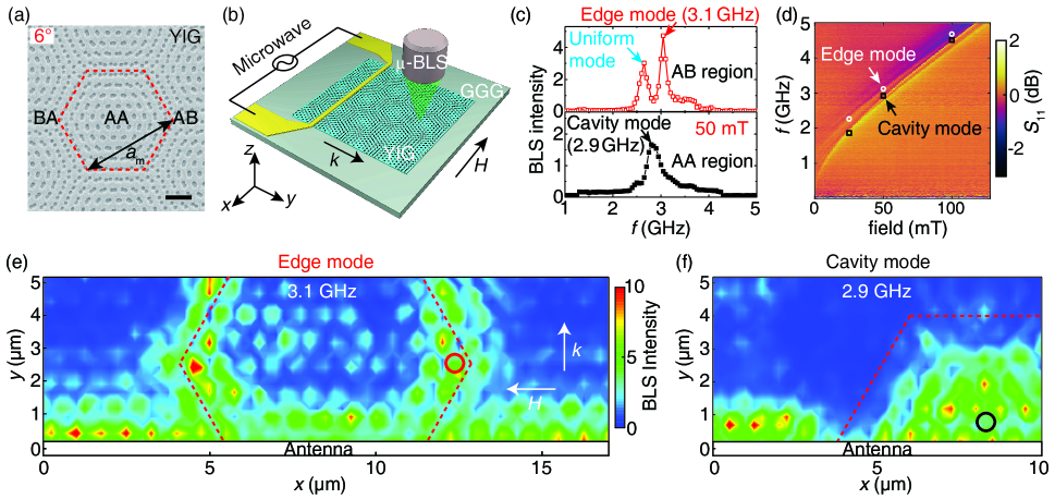
Figure 1: (a) Scanning electron microscope (SEM) image of a moiré magnonic lattice based on YIG grown on a GGG substrate with a twist angle of 6^∘. The red dashed line indicates a moiré unit cell with commensurate AA region at its center and incommensurate AB (BA) region at its edge. Moiré lattice constant $a_{\rm m}$ is marked by the black arrow. Scale bar, 2 $\mu$m. (b) Schematics of spatially-resolved spin-wave measurement on moiré magnonic lattices based on $\mu$-BLS. Microwaves injected by a nanostripline antenna (gold line) excite spin waves with a wavevector $k$ perpendicular to the antenna. Magnetic field $H$ is applied along the antenna. (c) $\mu$-BLS signals detected as a function of frequency at the AB region [red circle in (e)] and AA region [black circle in (f)] with an applied field of 50 mT. (d) Spin-wave reflection spectra $S_{\rm 11}$ measured by the all-electrical spin-wave spectroscopy. White circles and black open squares: Field dependent edge and cavity mode frequencies detected by $\mu$-BLS, respectively. (e) Two-dimensional spin-wave intensity maps measured by $\mu$-BLS at 3.1 GHz. The center of the excitation antenna is defined as $y$ = 0. (f) Two-dimensional spin-wave intensity maps measured by $\mu$-BLS at 2.9 GHz. The red dashed lines are guide to the eyes for a moiré unit cell. The applied field is set at 50 mT.

In this Letter, we experimentally investigate spin-wave propagation in a moiré magnonic lattice and observe topological spin-wave edge states at the boundary of a moiré unit cell with an optimal combination of the twist angle and applied magnetic field. Two antidot sublattices with a relative twist angle are merged in a single yttrium iron garnet (YIG) thin film, thus forming a moiré magnonic lattice [Fig. 1(a)]. Here we choose a triangle lattice to resemble the hexagonal lattice symmetry of graphene Cao2021 ; TYu2021 while the results may apply to other types of lattice Chen2022 . Antidot lattices Neusser2010 ; Duerr2011 ; Gross2021 are used to form the moiré magnonic crystals instead of dot arrays Tacchi2011 to preserve large continuous film areas for efficient spin-wave guiding. We employ micro-focused Brillouin light scattering ($\mu$-BLS) [Fig. 1(b)] to directly visualize two types of spin-wave modes in a moiré magnonic lattice, namely, i) Spin waves propagating along the edges of a moiré unit cell [Fig. 1(e)], which we refer to henceforth as moiré edge modes or simply edge modes. ii) Spin waves strongly confined at the center of a moiré unit cell [Fig. 1(f)], which is referred to as moiré cavity modes or simply cavity modes in analogy to its photonic counterpart Dong2021 ; Mao2021 . The most intense edge mode arises in the moiré magnonic lattice at an optimal twist angle of 6^∘ with an applied field of 50 mT. Micromagnetic simulations indicate that the edge mode emerges within the original band gap XWang2017 ; Bos2020 ; Dai2021 and at the intersection between two magnon branches. By extending the theoretical tools in magnon-photon Okamoto2020 and magnon-phonon Okamoto20202 systems, we derive the Berry curvature induced by the magnon-magnon coupling with dipolar interactions Shindou2013 that reveals a nontrival topology of the chiral spin-wave edge modes. The moiré edge modes reported here are related but still distinctive from high-energy magnons ($\sim$meV) in van der Waals materials usually studied with large facilities such as neutron scattering Yuan2020 , at ultra-low temperatures below 1 K Gan_arXiv and with high magnetic fields typically of a few Tesla Dai2021 . In this study, spin-wave edge modes are excited at GHz frequencies, detected at room temperature and tunable with a moderate magnetic field, and are thus readily compatible with existing on-chip electronics and microwave technology providing new opportunities towards applications in spin-wave-based computing Chumak2022 and wireless communications Harris2022 .

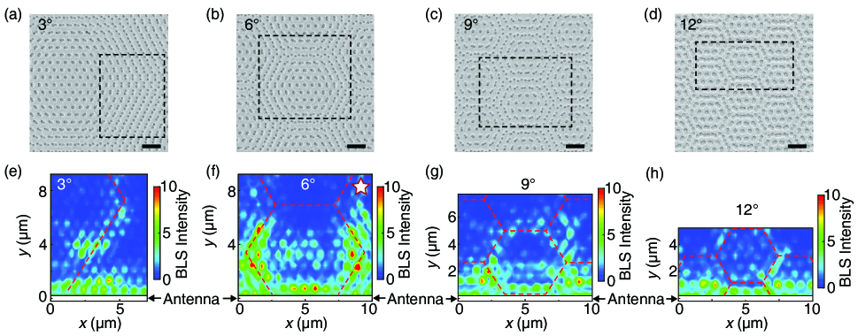
Figure 2: (a)-(d) SEM images of moiré magnonic lattices with twist angles of 3^∘, 6^∘, 9^∘ and 12^∘, respectively. Black dashed windows are the $\mu$-BLS scanning regions, e.g. 10 $\mu$m $\times$ 10 $\mu$m for (b). All scale bars are 2$\,\mu$m. (e-h) Two-dimensional spin-wave intensity maps measured by $\mu$-BLS at a twist angle of 3^∘, 6^∘, 9^∘ and 12^∘ with an excitation frequency of 3.10 GHz and applied magnetic field of 50 mT. Red dashed lines are guide to the eyes for moiré unit cells. The white star marks the edge mode profile around the optimal twist angle or ‘magic angle’.

II II. Sample information and spin-wave measurements

The moiré magnonic lattices were formed using two sets of antidot triangle lattices meshed into one single YIG layer with different values of the twist angle $\theta$ as shown in Fig. 1(a). One single antidot lattice acts as a conventional magnonic lattice with a lattice constant $a$ = 800 nm and an antidot diameter of 260 nm. The moiré magnonic lattices were fabricated using ebeam lithography and ion beam etching based on an 80 nm-thick YIG film grown by magnetron sputtering at room temperature on 0.5 mm-thick (111) gadolinium gallium garnet (GGG) substrates and annealed at 800^∘C for 4 hours in 1.12 Torr oxygen, subsequently. A gold stripline antenna with a width of 400 nm was then integrated on the moiré magnonic lattices to excite spin waves with a microwave source generator. The nanostripline (NSL) provides a broadband excitation Ciu2016 ; vanderSar2020 in wavevector space that covers the first Brillouin zone (BZ) boundary of the magnonic crystal as shown in the antenna fast Fourier transformation (FFT) in the Supplementary Material (SM) Fig. S1 SI . Spin-wave propagation was probed by $\mu$-BLS [Fig. 1(b)] with a spatial resolution of approximately 250 nm Madami_book (see Appendix A). The $\mu$-BLS signals were measured as a function of excitation frequency in the AB (incommensurate) and AA (commensurate) regions as shown in Fig. 1(c) with an applied field of 50 mT parallel to the antenna. Apart from the uniform mode around 2.7 GHz, associated with the spatially uniform mode excited through the lattice, another intense peak is detected at 3.1 GHz propagating along the edges of a moiré unit cell as shown in Fig. 1(e) with a contour profile. The raw data of Fig. 1(e) with a grid profile are presented in the SM Fig. S2 SI for comparison. The moiré edge mode is highly sensitive to its excitation frequency (see SM Section III SI ). At the black circle in Fig. 1(f), an additional mode is observed around 2.9 GHz which is identified as a moiré cavity mode. The spatial mapping of a full moiré unit cell is presented in SM Fig. S4 SI . Both moiré edge and cavity modes detected by the $\mu$-BLS have clear field dependence [Fig. 1(d)], that agrees well with modes detected by the all-electrical spin-wave spectroscopy based on a vector network analyzer (see Appendix B).

Figures 2(a)-(d) present the SEM images of moiré magnonic lattices with different twist angles $\theta$ of 3^∘, 6^∘, 9^∘ and 12^∘, for which the moiré lattice constants $a_{\text{m}}$ are calculated to be 15.3 $\mu$m, 7.6 $\mu$m, 5.1 $\mu$m and 3.8 $\mu$m with a single-layer periodicity $a$ = 800 nm, based on the simple estimation $a_{\text{m}}$=a/$\theta$ ($\theta$ in units of $rad$) Dong2021 . NSL antennas for microwave excitation are placed at the bottom of the black dashed windows [Figs. 2(a-d)] within which the $\mu$-BLS mappings are measured and shown in Figs. 2(e)-(h). Spin-wave moiré edge mode profiles are found to depend critically on two key parameters, i.e. the twist angle $\theta$ and the applied magnetic field $H$ (see Table 1 in the SM Section V SI for the full diagram). At a certain magnetic field of 50 mT, moiré edge mode profiles are measured for different twist angles of 3^∘, 6^∘, 9^∘ and 12^∘ as shown in Figs. 2(e)-(h) with the same excitation frequency of 3.10 GHz. The edge mode profile optimizes around 6^∘ in terms of both $\mu$-BLS signal intensity and peak linewidth as shown in the SM Fig. S5 SI . This indicates that the twist angle of 6^∘ can be considered as a ‘magic angle’ of the magnonic moiré lattice for a given magnetic field of 50 mT in analogy with those in electronic Bistritzer2011 ; Cao2018 and photonic Dong2021 ; Mao2021 moiré systems. However, the ‘magic angle’ is not fixed at 6^∘ but sensitive to the external magnetic field, e.g. at 40 mT, the magic angle is 3^∘ while at 60 mT it becomes 9^∘ as indicated by stars in Table 1 of the SM Section V SI . The applied field may tune the local magnetization alignment at the “top” and “bottom” layers of the moiré superlattice that is known to affect the interlayer magnon-magnon coupling strength Klingler2018 ; Chen2018 ; Qin2018SR ; Shiota2020 . Just as the magic angle depends on the interaction strength in electronic moiré systems Pan2020 and on the interlayer separation in photonic moiré crystals Wang2020 , the magic angle in magnonic moiré lattices depends on the interlattice coupling strength that can be tuned by an applied magnetic field.

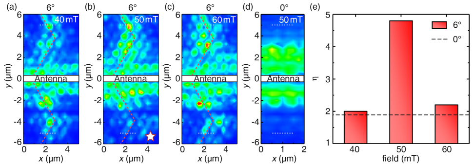
Figure 3: Spin-wave edge mode profiles measured by $\mu$-BLS on a magnetic moiré lattice with a twist angle of 6^∘ with an external magnetic field of 40 mT (a), 50 mT (b) and 60 mT (c) applied parallel to the stripline antenna (white bar). The excitation frequency is set at 3.1 GHz. The white star denotes the chiral edge mode profile at an optimal applied field value of 50 mT at a fixed twist angle of 6^∘. (d) Spin-wave spatial profile measured by $\mu$-BLS on a conventional magnonic crystal without moiré pattern, i.e. zero twist angle with an applied field of 50 mT. The antennas used in (a-d) are of the same design, i.e. 400 nm-wide NSL. (e) Chirality ratio $\eta=I_{+k}/I_{-k}$ extracted from the experimental data for 6^∘ (red columns) and 0^∘ (black dashed line) at a distance of 5 $\mu$m from the antenna [white dotted lines in (a-d)].

On the other hand, at a certain twist angle for instance of 6^∘, one can find an optimal applied field (‘magic field’, if one will) for generating the most intense edge mode profiles as shown in Figs. 3(a)-(c). Here, another salient feature of the moiré edge mode is observed as its chirality in the sense that spin waves propagating towards two opposite directions ($+k$ and $-k$) exhibit different intensities. To evaluate the strength of this effect, we introduce a chirality ratio as $\eta=I_{+k}/I_{-k}$ where $I_{+k}$ and $I_{-k}$ are spin-wave intensities measured by $\mu$-BLS with positive and negative wavevectors $+k$ and $-k$, respectively. At a fixed twist angle of 6^∘, spin-wave edge modes measured at different applied fields (40 mT, 50 mT and 60 mT) show different chiral propagation behavior [Figs. 3(a-c)], from which the chirality ratios $\eta$ are extracted and presented as the red columns in Fig. 3(e). At the optimal field (or ‘magic field’) of 50 mT, the chirality ratio maximizes at a value of 4.8 (see SM Fig. S6 SI for the raw data), whereas smaller chirality ratios of 2.0 and 2.2 are found for 40 mT and 60 mT, respectively. Meanwhile, it is also known that a stripline antenna can introduce a certain chirality Demi2009 ; TYu2021b ; vanderSar2021 when exciting spin waves in a Damon-Eshbach configuration DE1961 ; Yamamoto2019 ; Mohseni2019 . To assess and distinguish the chirality induced by the antenna and by the moiré system, we conduct a control measurement with the same antenna on a non-moiré magnonic crystal, i.e. $\theta$ = 0^∘ at 50 mT as shown in Fig. 3(d), where a weak chirality is observed with $\eta\simeq 1.8$ [dashed line in Fig. 3(e)] attributed purely to the antenna excitation Demi2009 ; TYu2021b ; vanderSar2021 . The significantly enhanced chirality ratio at the optimal magnetic field and twist angle may arise from the magnonic band modification by the moiré pattern Chen2022 .

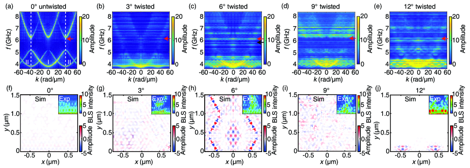
Figure 4: (a) Magnonic band structure calculated by micromagnetic simulations for the untwisted antidot magnonic lattice with a periodicity of 100 nm, where the dashed white lines are the BZ boundaries. Spin-wave propagation profile in simulations for the mode slightly below the upper band marked by the red arrow (6.10 GHz) is presented in (f). The inset shows the experimental results taken by $\mu$-BLS on the untwisted magnonic lattices for comparison. (b-e) Magnonic band structure from simulation for the moiré magnonic lattice with a twist angle of 3^∘, 6^∘, 9^∘, 12^∘, where the red arrow denotes the edge mode at 6.10 GHz whose propagation profile is shown in (g-h), respectively. The insets show the edge mode profile measured by $\mu$-BLS on a sample with a lattice contant of 800 nm. The black arrow in (c) denotes the cavity mode at 5.90 GHz. The magnetic fields in these simulations are set as 50 mT.

III III. Micromagnetic simulations and theoretical analysis

To further understand the spin-wave edge modes observed by $\mu$-BLS spectroscopy, we perform micromagnetic simulations for structures with twist angles of 0^∘, 3^∘, 6^∘, 9^∘ and 12^∘ based on OOMMF oommf . In order to limit the computing time, we considered antidot magnonic lattices with a periodicity of 100 nm instead of 800 nm for real samples. It is worth noting that the magnon band structure and edge mode spatial profile simulated for 800 nm is primarily consistent with those for 100 nm but demands a significantly longer time for computing even with lower wavevector resolution (see SM Section VIII SI ). For simplicity, the simulation is set in an area (4 $\mu$m$\times$12 $\mu$m) of a 100 nm-period antidot triangle lattice with a hole diameter of 50 nm. The external magnetic field of 50 mT is set along $x$ direction (see Appendix C for more details and parameters). The magnonic band structure is then obtained from simulations first for the untwisted magnonic lattice with $\theta$ = 0^∘ [Fig. 4(a)], where magnonic band gaps Neusser2010 ; Tacchi2011 ; Barman2021 are clearly observed between 5.15 GHz and 6.25 GHz. The spin-wave mode at 6.10 GHz (red arrows) locates within the forbidden band gap (see Fig. 4(a) and its zoom-in spectra in the SM Fig. S8 SI ) and therefore can hardly be excited as shown in Fig 4(f). With a twist angle of 6^∘ [Fig. 4(c)], the magnonic band structure is completely modified after complex mode hybridization. Instead of a clear band gap, several mini-flatbands Chen2022 [red and black arrows in Fig. 4(c)] arise near the first BZ boundaries due to the magnon-magnon hybridization Chen2018 ; Klingler2018 ; Qin2018SR ; Shiota2020 , as illustrated in Fig. 5(d). The moiré edge mode emerges at 6.10 GHz (red arrow) with its spatial profile shown in Fig. 4(h), whereas the moiré cavity mode appears at 5.80 GHz (black arrow) with its spatial profile shown in the SM Fig. S9(a) SI . However, when the twist angle is tuned up to 12^∘, the mini-flatband starts to disappear by losing its flatness [Fig. 4(e)], and consequently, the quality of moiré edge mode deteriorates severely [Fig. 4(j)]. The cavity mode around 5.80 GHz [black arrows in Figs. 4(c)] is well-confined at the AA region for $\theta$ = 6^∘, but becomes more scattered for $\theta$ = 12^∘ as shown in the SM Fig. S9(b) SI . The formation of the mini-flatband appears as a result of mode hybridization induced by the interlayer magnon-magnon coupling Chen2018 ; Klingler2018 ; Qin2018SR ; Shiota2020 between two magnonic-crystal layers Chen2022 in analogy to flat bands formed by interlayer interaction in its electronic Bal2020 and photonic Dong2021 counterparts.

To investigate the origin of the edge mode, we take the real-space simulation results of Fig. 4(h) and perform fast Fourier transformation (FFT) at the AB regions in which edge modes locate as shown in Fig. 5(a). The magnon edge modes correspond to two strong intensities in reciprocal space at the intersection between the flatband and an ordinary propagating mode as indicated by the red arrows in Fig. 5(b) and shown in a blow-up dispersion in Fig. 5(c). The actual formation process of edge mode and flatbands may be rather complicated and requires more sophisticated theoretical investigation in the future. Here we consider a simplified scenario for the edge mode formation as illustrated in Fig. 5(d), where the magnonic upper band of the ‘bottom’ layer (red dashed line) hybridizes with that of the ‘top’ layer (blue dashed lines) twisted with respect to the ‘bottom’ one and form a new magnon band structure with edge modes located at the turning point. To enable further theoretical calculation, we assume that the hybridization process occurs in two steps: 1) The minimums of the upper bands of both layers (bottom of red and blue dashed lines) first form a “flatband” $\omega_{0}$ Chen2022 . 2) The flatband $\omega_{0}$ couples subsequently with the propagating mode $\omega_{\text{m}}$. The second step is illustrated in Fig. 5(e). The simulation results in Fig. 5(c) suggest that the edge mode corresponds to the pronounced crossing point between a flatband mode and a propagating mode with a positive group velocity. Based on this observation, we consider the edge mode result from the mode hybridization shown in Figs. 5(e) and (f). In the following, we demonstrate theoretically that the upper branch $\omega_{+}$ formed by hybridization exhibits a nontrivial topology with a Chern number $Ch_{+}=-1$ and the edge mode appears in the band gap formed after the hybridization.

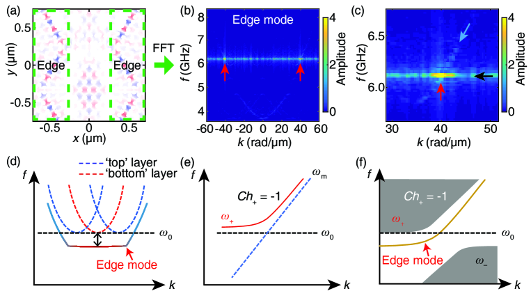
Figure 5: (a) Simulated spatial spin-wave intensity mappings on the moiré magnonic lattices with a twist angle of 6^∘ at the edge-mode frequency of 6.10 GHz. The edge mode regions within the green dashed squares are taken for the FFT to generate the intensity distribution of the spin-wave dispersion in (b). The red arrows denote the pronounced excitation of the edge modes. (c) The zoom-in plot indicates that the edge mode (red arrow) appears at the intersection of the flatband (black arrow) and a propagating mode (light blue arrow). (d) Sketches for the formation of the mini-flatband and edge mode resulted from mode hybridization of upper bands of two magnonic crystals twisted with respect to one another. The edge mode emerges slightly below the bottom of the upper bands ($\omega_{0}$) as indicated by the red arrow. (e) Simplified scenario for magnon-magnon coupling between the upper band bottom ($\omega_{0}$) and propagating mode ($\omega_{\rm m}$) considered in the theoretical analysis. Chern number ($Ch_{+}$) for the hybridized upper branch $\omega_{+}$ is calculated to be $-1$. (f) Schematics of the emergent chiral edge mode in the band gap between $\omega_{+}$ and $\omega_{-}$.

We adopt the theoretical approach used in Ref. Okamoto2020 ; Okamoto20202 to study the Berry curvature induced by the magnon-photon hybridization and apply it to the magnon-magnon coupling scenario of this work. Here, an initial approximation is necessary where we separate the merged moiré magnonic superlattice into two adjacent antidot sublattices twisted with one another (see its illustration in SM Fig. S10 SI ), so that the coupling between two twisted lattices can be considered as interlayer magnon-magnon coupling mediated by the dipolar interaction Chen2018 ; Shiota2020 . A simplified model is considered where only the coupling between the neighbouring antidots with the same registry in each layer is calculated. Each antidot can be regarded as a macroscopic magnetic dipole under an in-plane field suggested by the simulation shown in the SM Section XII SI . After a lengthy calculation (see Appendix D), we obtain the Berry curvature $\Omega_{z,+}\left(k\right)$ for the hybridized mode $\omega_{\rm+}$ [Fig. 5(e)] as,

$$\Omega_{z,+}(k)=\frac{1}{k}\frac{\partial}{\partial k}\left[\frac{\epsilon_{\rm d}^{2}(\epsilon_{+}^{3}+\epsilon_{+})}{2\epsilon_{\rm d}^{2}(2\epsilon_{+}^{2}-1)+2\epsilon_{\rm m}(\epsilon_{+}^{2}-1)^{2}}\right],$$ (1)

where $\epsilon_{+}=\omega_{+}/\omega_{0}$, $\epsilon_{\rm m}=\omega_{\rm m}/\omega_{0}$, and $\epsilon_{\rm d}=\omega_{\rm d}/\omega_{0}$ with $\omega_{\rm d}$ represents the term associated with the dipolar interaction (see Appendix D). The Chern number $Ch_{+}$ for the edge mode at the hybridized point of $\omega_{+}$ can then be calculated by the integral of the Berry curvature [Eq. 1] over the two-dimensional wavevector space Thouless1982 using,

$$Ch_{+}=\frac{1}{2\pi}\int_{\rm BZ}\Omega_{z,+}(k)dk_{x}dk_{y}.$$ (2)

The Chern number $Ch_{\rm+}$ for the hybridized magnon mode $\omega_{\rm+}$ can be derived based on Eq. 2 to be $Ch_{\rm+}=-1$ (see Appendix D). This reveals the non-trivial topological nature Shindou2013 of the magnon edge mode in moiré magnonic lattices. Through the calculation process, the external magnetic field can tune the local magnetization orientation and affect the interlattice dipolar interaction that may lead to a change on the Berry curvature of the hybridized system. As a result, the chiral edge mode is responsive to the applied magnetic field as observed in experiments [Figs. 3(a-c)], which resonates with a recent theoretical study showing tunable magnonic Chern bands with an external magnetic field Luqiao2022 based on dipolar interaction in multilayers. Considering the fact that the mini-flatband $\omega_{0}$ depends critically on the twist angle $\theta$, the non-trivial topological spin-wave edge modes emerge at a certain combination of the twist angle $\theta$ and magnetic field $H$, which accounts for the spin-wave edge modes observed by $\mu$-BLS in experiments (see Table 1 in the SM Section V SI ). The microscopic mechanism of the nontrivial topological spin-wave edge mode is the dipolar interaction Shindou2013 ; Li2018 which relies on the relative position of two spins (tunable by twist angle $\theta$) and their spin orientations (tunable by magnetic field $H$) Shen2020 . Our conclusion that dipolar interaction is responsible for our observation resonates with the origin of topological spin-wave edge modes theoretically predicted in other magnonic lattices Shindou2013 ; Li2018 .

IV IV. Discussion and Conclusion

The observed topological spin-wave edge modes emerge at the edge of a moiré unit cell that is analogous to the topological mosaics predicted in twisted van der Waals bilayers Tong2017 . Remarkably, if one rotates the wavevector excitation towards the $M$ point instead of the $K$ point symmetry in the reciprocal space, spin waves tend to propagate along the edge of the entire lattice referred to as ‘bulk edge mode’ in the simulation results of Fig. S12 in the SM SI . In this work, however, we focus on investigating the moiré edge mode [Fig. 1(e)] rather than the bulk edge mode which we leave for future experimental and theoretical investigations. Further simulation results reveal that the quality of the edge mode relies also on the diameter of the antidots as shown in the SM Fig. S13 SI . This indicates that the filling factor is an additional parameter for the generation of non-trivial topological magnon modes comparable with the important role of filling ratio in a topological phononic system as demonstrated recently in a numerical study Pirie2022 . Although we attribute the topological origin of our observation to be primarily interlattice dipolar interaction, the interlayer exchange (RKKY) interaction Parkin1990 and Dyzaloshinskii-Moriya interaction Gam2021 in magnetic moiré bilayer systems may also play a role in forming spin-wave edge modes and is challenging while interesting to investigate in the future for example theoretically using tight-binding models Shen2018 ; Eck2022 .

In conclusion, spin-wave edge modes and cavity modes are experimentally demonstrated in moiré magnonic lattices by micro-focused BLS. The edge modes are observed at the boundary of a moiré unit cell while the cavity modes are localized within the center of the moiré unit cell. With an applied field of 50 mT, the moiré edge mode is most intense at a magic twist angle of 6^∘. The dependence of the ‘magic angle’ on the applied magnetic field indicates that the dipolar interaction between the twisted magnonic sublattices plays an important role in the formation of the moiré edge modes. The magnetic field offers an additional degree of freedom for tuning the magnon edge mode on top of the twist angle and thus provides more versatility to magnonic moiré devices. The micromagnetic simulations show that the edge mode arises at the crossing point between a moiré flatband and a propagating magnon branch near the first BZ boundary. Estimates of the Berry curvature for magnon-magnon coupling further confirms that the dipolar interaction is the key mechanism of magnon edge modes that exhibit a non-trivial topological nature with a non-zero integral Chern number. The moiré spin-wave edge modes observed in this work, as the magnonic counterpart of the magic-angle electronic and photonic systems, open an emergent research direction of moiré magnonics. The use of topologically protected magnon edge modes will greatly expand the functionalities of magnonic devices for information processing.

V Acknowledgments

We wish to acknowledge the support by the National Key Research and Development Program of China Grant No. 2022YFA1402801, by NSF China under Grant Nos. 12074026, 52225106 and U1801661, by China Scholarship Council (CSC) under Grant No. 202206020091 and by Shenzhen Institute for Quantum Science and Engineering, Southern University of Science and Technology (Grant No. SIQSE202007). M.M. and G.G. acknowledge financial support from the Italian Ministry of University and Research through the PRIN-2020 project entitled ‘The Italian factory of micromagnetic modelling and spintronics’, cod. 2020LWPKH7.

VI Appendix A: Micro-focused Brillouin light scattering

Brillouin light scattering spectroscopy is based on the inelastic scattering of light by thermally or $rf$ excited spin waves. A diffraction limited spatial resolution of about 250 nm is reached by employing a single-mode solid-state laser with a wavelength of 532 nm, at normal incidence, using a microscope objective with numerical aperture 0.75. A (3+3)-pass tandem Fabry-Pérot interferometer is used to analyze the inelastically scattered light. A nanopositioning stage allows to position the sample with a precision down to 10 nm on all three axes. A DC/AC electrical probe station ranging from DC up to 20 GHz is used for spin-wave pumping. The microwave power is set at +18 dBm on the rf generator output.

VII Appendix B: All-electrical spin wave spectroscopy

The all-electric spin-wave spectroscopy consists of Rohde $\&$ Schwarz VNA with frequency range from 10 MHz to 40 GHz and a U-shaped electric-controlled external magnets. The YIG film is put between two magnetic poles. The external magnetic field is parallel with the NSL antenna and perpendicular to the spin-wave wavevectors. The integrated electrodes of the antenna on the top of moiré magnonic crystals are connected to the VNA via the microwave probes and cables. Therefore, the microwave currents can be injected into the excitation antennas and we measure the reflection spin-wave spectra of the nanostructured moiré magnonic crystals with sweeping the external magnetic field from -150 mT to 150 mT, after first saturating the film at -300 mT. The IF bandwidth is set to be 1 kHz.

VIII Appendix C: Micromagnetic simulations

The OOMMF (http://math.nist.gov/oommf) program is used for the micromagnetic simulations. Two-dimensional periodical boundary condition is considered in the simulation. The size of the single mesh cell is 5 nm$\times$ 5 nm. Two twisted triangle magnonic crystals are meshed into one layer to form the moiré pattern. We set the saturation magnetization $M_{\rm S}$= 140 kA/m, damping $\alpha$=10^-4 and the exchange coefficient $A$=3.7$\times$10^-12 J/m for YIG films. A 20 nm-wide stripline antenna is considered with a dynamic field in $x$ direction, which is described by ($H_{\rm ex}=h_{0}\sin(2\pi f(t-t_{0}))/(2\pi f(t-t_{0}))$), where the excitation field $h_{0}$=2 mT, $f$=20 GHz and $t_{0}$=100.1 ps. The dynamic field contains same excitation strength from 0 to $f$ GHz. The external magnetic field of 50 mT is set along $x$ direction, which is perpendicular to the wavevector direction along $y$. The magnetization ground state is calculated by minimizing the total energy of the YIG moiré magnonic crystals, based on which the magnetization dynamics is simulated for 1050 equidistant times with a time step of 25 ps. We then perform the two-dimensional fast Fourier transformation along $y$ direction to obtain the magnon band structures. For single-frequency excitation, we use $H_{\rm ex}=h_{0}\sin(2\pi f_{\rm fixed}(t-t_{0}))$, where $f_{\rm fixed}$ is the fixed excitation frequency. The spatial maps present the $x$ component of the magnetization dynamics at a certain time point.

IX Appendix D: Theoretical calculations

Taking into account the dipolar interaction in the magnonic moiré lattices, we utilize Landau-Lifshitz equations to analyze the magnetization dynamics as

$$\frac{d\bm{m}}{dt}=-\gamma\mu_{0}\bm{m}\times\left(\bm{H}_{{0}}+\bm{H}_{{\rm fb}}+\bm{H}_{{\rm dip}}\right),$$ (3)

$$\frac{d\tilde{\bm{m}}}{dt}=-\gamma\mu_{0}\tilde{\bm{m}}\times\left(\bm{H}_{{0}}+J_{0}\nabla^{2}\tilde{\bm{m}}+\tilde{\bm{H}}_{{\rm dip}}\right).$$

Here, $\bm{H}_{0}$ is the external magnetic field, $\bm{H}_{\rm fb}$ is the phenomenological field which creates a moiré flat band, $J_{0}$ is the exchange stiffness. In this appendix, the lattice-mode parameters are marked with a tilde. Since we only concern about the eigen-frequencies, we disregard the damping terms.

Then we estimate the hybridization of the lattice mode and mini-flat band. The Hamiltonian of interlayer dipole-dipole interaction under our approximation reads

$$\mathcal{H}_{\rm dip}=\frac{\mu_{0}}{2}\sum_{i\neq j}\frac{R_{ij}^{2}\bm{m}_{i}\cdot\bm{m}_{j}-3\left(\bm{R}_{ij}\cdot\bm{m}_{i}\right)\cdot\left(\bm{R}_{ij}\cdot\bm{m}_{j}\right)}{R_{ij}^{5}},$$ (4)

where $\bm{R}_{ij}$ represents the dislocations of antidots, and for nearest neighbors, we define $R_{ij}=R$. Dipolar fields $\bm{h}_{\rm dip}$ and $\tilde{\bm{h}}_{\rm dip}$ arises from this Hamiltonian. The total dipolar field of a macroscopic dipole is represented by $\bm{H}_{\rm dip}$, whose scale is accumulated by the antidot’s volume. As mentioned before, we only consider the nearest neighbor’s contribution. The dipolar effective field $\bm{H}_{\rm dip}$ can be estimated by $\bm{H}_{\rm dip}=\frac{1}{4}\bm{h}_{\rm dip}\cdot\pi\Phi^{2}t,$ where $t$ is the thickness of the film and $\Phi$ is the diameter of the holes. For antidots from two different layers locating at the moiré unit cell edge, this parameter $R$ could be written approximately as:

$$R\cong\frac{\lambda}{2}\theta_{{\rm twist}}=\frac{a}{2\theta_{{\rm twist}}}\cdot\theta_{{\rm twist}}=\frac{a}{2}$$ (5)

where the $\theta_{\rm twist}$ is the twisted angle between two layers. Therefore, the static dipolar field is estimated by $H_{\rm dip}=\tilde{H}_{\rm dip}=\frac{M_{\rm S}}{16R^{3}}\Phi^{2}t$. It affects the orientations of antidots’ magnetizations, which means that the static orientation of $\bm{m}$ and $\tilde{\bm{m}}$ might be not inherently following the direction of the external magnetic field. To make the total energy minimum under the coexistence of forementioned dipolar interaction, local shape anisotropy, and external field, it comes to an equilibrium static state with spatial distributions. In other words, the external field $\bm{H}_{0}$ enforces magnetization to be fixed, while it is not strong enough, with respect to the static dipolar field, to predominate the direction of saturated magnetization orientations. We define the angle between magnetization orientation and the external field as $\beta$. Thus, equations of motion (EOM) describing the antidot moiré spin waves are written as:

$$\left\{\begin{array}[]{ll}\frac{dm_{x}}{dt}=-\gamma\mu_{\rm 0}\left[H_{\rm 0}\cos\beta+H_{\rm{fb}}-H_{\rm{dip}}\left(1-3\sin^{2}\phi\right)\right]m_{y}-\gamma\mu_{\rm 0}H_{\rm{dip}}\tilde{m}_{y},\\ \frac{dm_{y}}{dt}=\gamma\mu_{\rm 0}\left[H_{\rm 0}\cos\beta+H_{\rm{fb}}-H_{\rm{dip}}\left(1-3\sin^{2}\phi\right)\right]m_{x}+\gamma\mu_{\rm 0}H_{\rm{dip}}\left(1-3\cos^{2}\phi\right)\tilde{m}_{x}+C,\\ \frac{d\tilde{m}_{x}}{dt}=-\gamma\mu_{\rm 0}\left[H_{\rm 0}\cos\beta+J_{\rm 0}M_{\rm{S}}|k|^{2}-\tilde{H}_{\rm{dip}}\left(1-3\sin^{2}\phi\right)\right]\tilde{m}_{y}-\gamma\mu_{\rm 0}\tilde{H}_{\rm{dip}}m_{y},\\ \frac{d\tilde{m}_{y}}{dt}=\gamma\mu_{\rm 0}\left[H_{\rm 0}\cos\beta+J_{\rm 0}M_{\rm{S}}|k|^{2}-\tilde{H}_{\rm{dip}}\left(1-3\sin^{2}\phi\right)\right]\tilde{m}_{x}+\gamma\mu_{\rm 0}\tilde{H}_{\rm{dip}}\left(1-3\cos^{2}\phi\right)m_{x}+C,\end{array}\right.$$ (6)

where $\phi=\pi/6+\beta$. In these equations, there are inhomogeneous terms $C$ which shouldvanish since we are looking for the linear response. Thus, we find that the angle $\beta$ obeys the following equation:

$$C=-H_{0}M_{{\rm S}}\sin\beta+3H_{{\rm dip}}M_{{\rm S}}\sin\phi\cos\phi=0.$$ (7)

Then, we let $\bm{x}_{k}=\left(m_{x},m_{y},\tilde{m}_{x},\tilde{m}_{y}\right)^{\intercal}$ represent the wavefunction of spin waves. Our EOM could be transformed as:

$$i\frac{d\bm{x}_{k}}{dt}=\mathcal{H}_{\rm{eff}}\cdot\bm{x}_{k}.$$ (8)

Then, we define parameters as follows:

$$\left\{\begin{array}[]{l}\omega_{\rm d}=\gamma\mu_{\rm 0}H_{\rm dip},\\ \omega_{\rm 0}=\gamma\mu_{\rm 0}\left(H_{\rm 0}+H_{\rm fb}\right)-\omega_{\rm d}\left(1-3\sin^{2}{\phi}\right),\\ \omega_{\rm m}=\gamma\mu_{\rm 0}\left(H_{\rm 0}+J_{\rm 0}M_{\rm S}\tilde{k}^{2}\right)-\omega_{\rm d}\left(1-3\sin^{2}{\phi}\right),\end{array}\right.$$ (9)

and under these definitions, our effective Hamiltonian reads

$$\mathcal{H}_{\rm{eff}}=\left(\begin{array}[]{cccc}0&-i\omega_{{\rm 0}}&0&-i\omega_{{\rm d}}\\ i\omega_{{\rm 0}}&0&i\omega_{{\rm d}}\left(1-3\cos^{2}\phi\right)&0\\ 0&-i\omega_{{\rm d}}&0&-i{\omega}_{{\rm m}}\\ i\omega_{{\rm d}}\left(1-3\cos^{2}\phi\right)&0&i{\omega}_{{\rm m}}&0\end{array}\right).$$ (10)

Nonetheless, this Hamiltonian could be spotted easily as a non-Hermitian one. Within a energy conservation system, the Hamiltonian should be Hermitian. This information implies a non-zero Berry curvature. Then we assume a Hermitian matrix $\sigma$ that,

$$\sigma=\left(\begin{array}[]{c c c c}0&-i&0&0\\ i&0&0&0\\ 0&0&0&-i\\ 0&0&i&0\end{array}\right),$$ (11)

and define $\mathcal{\tilde{H}}_{\rm{eff}}=\sigma\cdot\mathcal{H}_{\rm{eff}}$. Then $\mathcal{\tilde{H}}_{\rm{eff}}$ is Hermitian. Actually, it is real and symmetric, with,

$$\mathcal{\tilde{H}}_{\rm{eff}}=\left(\begin{array}[]{cccc}\omega_{\rm{0}}&0&\omega_{\rm{d}}\left(1-3\cos^{2}\phi\right)&0\\ 0&\omega_{\rm{0}}&0&\omega_{\rm{d}}\\ \omega_{\rm{d}}\left(1-3\cos^{2}\phi\right)&0&\omega_{\rm{m}}&0\\ 0&\omega_{\rm{d}}&0&\omega_{\rm{m}}\end{array}\right).$$ (12)

Now we want to calculate the topological parameters of hybridized bands. According to our experimental results, there is an exceptional point for external magnetic field that could generate edge modes. We intuitively assume that when $1-3\cos^{2}{\phi}=0$ the conditions might be exceptional. This assumption is not entirely precise but could reveal some nature about the internal mechanism of the field-dependent phase transition.

The external magnetic field modulate the spin orientations of antidots. From Eq. 7, we can analytically find out that the angle $\phi$’s relation to the external field strength $\bm{H}_{0}$. We note that $\phi=\phi(H_{0})$.

At this stage, the effective Hamiltonian in Eq. 12 is now,

$$\mathcal{H}_{\rm{eff}}^{\star}=\left(\begin{array}[]{cccc}0&-i\omega_{{\rm 0}}&0&-i\omega_{{\rm d}}\\ i\omega_{{\rm 0}}&0&0&0\\ 0&-i\omega_{{\rm d}}&0&-i{\omega}_{{\rm m}}\\ 0&0&i{\omega}_{{\rm m}}&0\end{array}\right).$$ (13)

The eigenvalue and eigenvector equations of the fixed effective Hamiltonian can be written as:

$$\sigma\cdot\omega\bm{x}_{{k}}=\mathcal{\tilde{H}}_{\rm{eff}}^{\star}\cdot\bm{x}_{{k}}.$$ (14)

By solving this equation, the eigenvalues of the fixed effective Hamiltonian are:

$$\omega_{\pm}^{2}=\frac{\omega_{{\rm 0}}^{2}+\omega_{{\rm m}}^{2}}{2}\pm\sqrt{\left(\frac{\omega_{{\rm 0}}^{2}-\omega_{{\rm m}}^{2}}{2}\right)^{2}+C_{{\rm d}}^{2}},$$ (15)

where $C_{\rm d}$ represents the coupling strength induced by the dipolar interaction,

$$C_{\rm d}^{2}=4\omega_{\rm d}^{2}\omega_{\rm 0}\omega_{\rm m}\sim g^{4}.$$ (16)

Substituting $\omega_{+}$ for the eigenvalue $\omega$ in the eigenvalue equation 14, we get the eigenfunction $\bm{x}_{k}$:

$$\bm{x}_{k}=\left(\begin{array}[]{c}-i\omega_{\rm{d}}\omega_{\rm+}^{2}\\ \omega_{\rm{d}}\omega_{\rm{0}}\omega_{\rm+}\\ -i\left[\omega_{\rm{d}}^{2}\omega_{\rm{0}}+\left(\omega_{\rm+}^{2}-\omega_{\rm{0}}^{2}\right)\omega_{\rm{m}}\right]\\ \omega_{\rm+}\left(\omega_{\rm+}^{2}-\omega_{\rm{0}}^{2}\right)\end{array}\right).$$ (17)

According to the methodology developed firstly by Refs Okamoto2020 ; Okamoto20202 , Berry curvature of the coupled waves can be represented as

$$\Omega_{{z},+}(k)=\frac{1}{k}\frac{\partial}{\partial k}\left(\frac{\tilde{\bm{x}}_{{k}}^{\dagger}\Sigma\tilde{\bm{x}}_{{k}}}{\tilde{\bm{x}}_{{k}}^{\dagger}\sigma\tilde{\bm{x}}_{{k}}}\right),$$ (18)

where $\Sigma=\rm{diag}\left(\emph{I}_{2\times 2},\emph{O}_{2\times 2}\right)$, with $I$ representing the unit matrix and $O$ representing zero matrix. Then, we can calculate the Berry curvature that,

$$\Omega_{\rm+}=\frac{1}{k}\frac{\partial}{\partial k}\left(\frac{\epsilon_{\rm{d}}^{2}\left(\epsilon_{\rm+}^{3}+\epsilon_{\rm+}\right)}{2\epsilon_{\rm{d}}^{2}\left(2\epsilon_{\rm+}^{2}-1\right)+2\epsilon_{\rm{m}}\left(\epsilon_{\rm+}^{2}-1\right)^{2}}\right).$$ (19)

We define $N(k)=\frac{\epsilon_{\rm{d}}^{2}\left(\epsilon_{\rm+}^{3}+\epsilon_{\rm+}\right)}{2\epsilon_{\rm{d}}^{2}\left(2\epsilon_{\rm+}^{2}-1\right)+2\epsilon_{\rm{m}}\left(\epsilon_{\rm+}^{2}-1\right)^{2}}$ by the equation 19. The upper branch $\omega_{+}$, which nearing but above the observed edge mode, is mainly studied in our following calculations. The Chern number can be written as

$$Ch_{+}=\frac{1}{2\pi}\int_{\rm BZ}\Omega_{+}\cdot k\cdot dk\cdot d\theta\cong N(\infty)-N(0).$$ (20)

When $k\rightarrow\infty$, we have $\omega_{+}\rightarrow\omega_{\rm m}\rightarrow\infty$, as well as $\omega_{\rm d}$ and $\omega_{\rm fb}$ are still finite constants, so that $\omega_{\rm 0}/\omega_{\rm m}=\omega_{\rm d}/\omega_{\rm m}=0,(k\rightarrow\infty)$. Therefore, we could simplify that

$$N(\infty) =\frac{\epsilon_{\rm{d}}^{2}\left(\epsilon_{\rm+}^{3}+\epsilon_{\rm+}\right)}{2\epsilon_{\rm{d}}^{2}\left(2\epsilon_{\rm+}^{2}-1\right)+2\epsilon_{\rm{m}}\left(\epsilon_{\rm+}^{2}-1\right)^{2}}$$ (21)

$$\sim\frac{\epsilon_{\rm{m}}^{3}\epsilon_{\rm{d}}^{2}}{2\left(\epsilon_{\rm{m}}^{2}\epsilon_{\rm{d}}^{2}+\epsilon_{\rm{m}}^{5}\right)}\rightarrow 0.$$

For the weak coupling regime as we assumed, when $k\rightarrow 0$, the approximation reads

$$\lim_{k\rightarrow 0}\omega_{+}=\omega_{\rm fb}.$$ (22)

Therefore, in this limitation, $\epsilon_{+}\rightarrow 1$. $N(0)$ could be calculated that,

$$N(0)=\lim_{\rm\epsilon_{\rm+}\rightarrow 1}\frac{\epsilon_{\rm{d}}^{2}\left(\epsilon_{\rm+}^{3}+\epsilon_{\rm+}\right)}{2\epsilon_{\rm{d}}^{2}\left(2\epsilon_{\rm+}^{2}-1\right)+2\epsilon_{\rm{m}}\left(\epsilon_{\rm+}^{2}-1\right)^{2}}=1.$$ (23)

Then, we have

$$Ch_{+}=N(\infty)-N(0)=-1,$$ (24)

which implies that the moiré edge mode has non-trivial topological properties.

References and Notes

- (1) R. Bistritzer, and A. H. MacDonald, Moiré bands in twisted double-layer graphene. Proc. Natl. Acad. Sci. USA 108, 12233-12237 (2011).
- (2) Q. Tong, H. Yu, Q. Zhu, Y. Wang, X. Xu, and W. Yao, Topological mosaics in moiré superlattices of van der Waals heterobilayers. Nat. Phys. 13, 356-362 (2017).
- (3) Y. Cao, V. Fatemi, S. Fang, K. Watanabe, T. Taniguchi, E. Kaxiras, and P. Jarillo-Herrero, Unconventional superconductivity in magic-angle graphene superlattices. Nature 556, 43-50 (2018).
- (4) A. T. Pierce, Y. Xie, J. M. Park, E. Khalaf, S. H. Lee, Y. Cao, D. E. Parker, P. R. Forrester, S. Chen, K. Watanabe, T. Taniguchi, A. Vishwanath, P. Jarillo-Herrero, and A. Yacoby, Unconventional sequence of correlated Chern insulators in magic-angle twisted bilayer graphene. Nat. Phys. 17, 1210-1215 (2021).
- (5) T. Li, S. Jiang, B. Shen, Y. Zhang, L. Li, Z. Tao, T. Devakul, K. Watanabe, T. Taniguchi, L. Fu, J. Shan, and K. F. Mak, Quantum anomalous Hall effect from intertwined moiré bands. Nature 600, 641-646 (2021).
- (6) X. Wang, C. Xiao, H. Park, J. Zhu, C. Wang, T. Taniguchi, K. Watanabe, J. Yan, D. Xiao, D. R. Gamelin, W. Yao, and X. Xu, Light-induced ferromagnetism in moiré superlattices. Nature 604, 468-473 (2022).
- (7) K. Dong, T. Zhang, J. Li, Q. Wang, F. Yang, Y. Rho, D. Wang, C. P. Grigoropoulos, J. Wu, and J. Yao, Flat bands in magic-angle bilayer photonic crystals at small twists. Phys. Rev. Lett. 126, 223601 (2021).
- (8) X.-R. Mao, Z.-K. Shao, H.-Y. Luan, S.-L. Wang, and R.-M. Ma, Magic-angle lasers in nanostructured moiré superlattice. Nat. Nanotechnol. 16, 1099-1105 (2021).
- (9) A. V. Chumak, V. Vasyuchka, A. A. Serga, and B. Hillebrands, Magnon spintronics. Nat. Phys. 11, 453-461 (2015).
- (10) J. Han, P. Zhang, J. T. Hou, S. A. Siddiqui, and L. Liu, Mutual control of coherent spin waves and magnetic domain walls in a magnonic device. Science 366, 1121-1125 (2019).
- (11) A. Barman, G. Gubbiotti, S. Ladak, A. O. Adeyeye, M. Krawczyk, J. Gräfe, C. Adelmann, S. Cotofana, A. Naeemi, V. I. Vasyuchka et al., The 2021 magnonics roadmap. J. Phys. Condens. Matter 33, 413001 (2021).
- (12) P. Pirro, V. I. Vasyuchka, A. A. Serga, and B. Hillebrands, Advances in coherent magnonics. Nat. Rev. Mater. 6, 1114-1135 (2021).
- (13) X. Zhang, L. Li, D. Weber, J. Goldberger, K. F. Mak, and J. Shan, Gate-tunable spin waves in antiferromagnetic atomic bilayers. Nat. Mater. 19, 838–842 (2020).
- (14) L. J. Cornelissen, J. Liu, R. A. Duine, J. B. Youssef, and B. J. van Wees, Long-distance transport of magnon spin information in a magnetic insulator at room temperature. Nat. Phys. 11, 1022-1026 (2015).
- (15) A. Khitun, M. Bao, and K. L. Wang, Magnonic logic circuits. J. Phys. D Appl. Phys. 43, 264005 (2010).
- (16) Q. Wang, M. Kewenig, M. Schneider, R. Verba, F. Kohl, B. Heinz, M. Geilen, M. Mohseni, B. Lägel, F. Ciubotaru, C. Adelmann, C. Dubs, S. D. Cotofana, O. V. Dobrovolskiy, T. Brächer, P. Pirro, and A. V. Chumak, A magnonic directional coupler for integrated magnonic half-adders. Nat. Electron. 3, 765-774 (2020).
- (17) Y.-H. Li, and R. Cheng, Moiré magnons in twisted bilayer magnets with collinear order. Phys. Rev. B 102, 094404 (2020).
- (18) C. Wang, Y. Gao, H. Lv, X. Xu, and D. Xiao, Stacking domain wall magnons in twisted van der Waals magnets. Phys. Rev. Lett. 125, 247201 (2020).
- (19) J. Chen, L. Zeng, H. Wang, M. Madami, G. Gubbiotti, S. Liu, J. Zhang, Z. Wang, W. Jiang, Y. Zhang, D. Yu, J.-Ph. Ansermet, and H. Yu, Magic-angle magnonic nanocavity in a magnetic moiré superlattice. Phys. Rev. B 105, 094445 (2022).
- (20) L. Zhang, J. Ren, J. S. Wang, and B. Li, Topological magnon insulator in insulating ferromagnet. Phys. Rev. B 87, 144101 (2013).
- (21) M. Elyasi, K. Sato, and G. E. W. Bauer, Topologically nontrivial magnonic solitons. Phys. Rev. B 99, 134402 (2019).
- (22) A. Mook, J. Henk, and I. Mertig, Edge states in topological magnon insulators. Phys. Rev. B 90, 024412 (2014).
- (23) S. A. Owerre, A first theoretical realization of honeycomb topological magnon insulator. J. Phys. Condens. Matter 28, 386001 (2016).
- (24) S. K. Kim, H. Ochoa, R. Zarzuela, and Y. Tserkovnyak, Realization of the Haldane-Kane-Mele model in a system of localized spins. Phys. Rev. Lett. 117, 227201 (2016).
- (25) T. Hirosawa, S. A. Díaz, J. Klinovaja, and D. Loss, Magnonic quadrupole topological insulator in antiskyrmion crystals. Phys. Rev. Lett. 125, 207204 (2020).
- (26) H. Kondo, and Y. Akagi, Dirac surface states in magnonic analogs of topological crystalline insulators. Phys. Rev. Lett. 127, 177201 (2021).
- (27) X.-G. Wang, Y.-Z. Nie, Q.-L. Xia, and G.-H. Guo, Dynamically reconfigurable magnonic crystal composed of artificial magnetic skyrmion lattice. J. Appl. Phys. 128, 063901 (2020).
- (28) E. V. Boström, T. S. Parvini, J. W. McIver, A. Rubio, S. V. Kusminskiy, and M. A. Sentef, Direct optical probe of magnon topology in two-dimensional quantum magnets. Phys. Rev. Lett. (to be published) arXiv:2207.04745
- (29) R. Shindou, R. Matsumoto, S. Murakami, and J. I. Ohe, Topological chiral magnonic edge mode in a magnonic crystal. Phys. Rev. B 87, 174427 (2013).
- (30) Y.-M. Li, J. Xiao, and K. Chang, Topological magnon modes in patterned ferrimagnetic insulator thin films. Nano Lett. 18, 3032-3037 (2018).
- (31) Y. Cao, D. Rodan-Legrain, J. M. Park, N. F Q. Yuan, K. Watanabe, T. Taniguchi, R. M. Fernandes, L. Fu, and P. Jarillo-Herrero, Nematicity and competing orders in superconducting magic-angle graphene. Science 372, 264-271 (2021).
- (32) T. Yu, D. M. Kennes, A. Rubio, and M. A. Sentef, Nematicity arising from a chiral superconducting ground state in magic-angle twisted bilayer graphene under in-plane magnetic fields. Phys. Rev. Lett. 127, 127001 (2021).
- (33) S. Neusser, G. Duerr, H. G. Bauer, S. Tacchi, M. Madami, G. Woltersdorf, G. Gubbiotti, C. H. Back, and D. Grundler, Anisotropic propagation and damping of spin waves in a nanopatterned antidot lattice. Phys. Rev. Lett. 105, 067208 (2010).
- (34) G. Duerr, M. Madami, S. Neusser, S. Tacchi, G. Gubbiotti, G. Garlotti, and D. Grundler, Spatial control of spin-wave modes in Ni80Fe20 antidot lattices by embedded Co nanodisks. Appl. Phys. Lett. 99, 202502 (2011).
- (35) F. Gross, M. Zelent, A. Gangwar, S. Mamica, P. Gruszecki, M. Werner, G. Schütz, M. Weigand, E. J. Goering, C. H. Back, M. Krawczyk, and J. Gräfe, Phase resolved observation of spin wave modes in antidot lattices. Appl. Phys. Lett. 118, 232403 (2021).
- (36) S. Tacchi, F. Montoncello, M. Madami, G. Gubbiotti, G. Carlotti, L. Giovannini, R. Zivieri, F. Nizzoli, S. Jain, A. O. Adeyeye, and N. Singh, Band diagram of spin waves in a two-dimensional magnonic crystal. Phys. Rev. Lett. 107, 127204 (2011).
- (37) X. S. Wang, Y. Su, and X. R. Wang, Topologically protected unidirectional edge spin waves and beam splitter. Phys. Rev. B 95, 014435 (2017).
- (38) E. V. Boström, M. Claassen, J. W. McIver, G. Jotzu, A. Rubio, and M. A. Sentef, Light-induced topological magnons in two-dimensional van der Waals magnets. SciPost Phys. 9, 061 (2020).
- (39) L. Chen, J.-H. Chung, M. B. Stone, A. I. Kolesnikov, B. Winn, V. O. Garlea, D. L. Abernathy, B. Gao, M. Augustin, E. J. G. Santos, and P. Dai, Magnetic field effect on topological spin excitations in CrI3. Phys. Rev. X 11, 031047 (2021).
- (40) A. Okamoto, R. Shindou, and S. Murakami, Berry curvature for coupled waves of magnons and electromagnetic waves. Phys. Rev. B 102, 064419 (2020).
- (41) A. Okamoto, S. Murakami, and K. Everschor-Sitte, Berry curvature for magnetoelastic waves. Phys. Rev. B 101, 064424 (2020).
- (42) B. Yuan, I. Khait, G.-J. Shu, F. C. Chou, M. B. Stone, J. P. Clancy, A. Paramekanti, and Y.-J. Kim, Dirac magnons in a honeycomb lattice quantum XY magnet CoTiO3. Phys. Rev. X 10, 011062 (2020).
- (43) S. C. Ganguli, M. Aapro, S. Kezilebieke, M. Amini, J. L. Lado, and P. Liljeroth, Visualization of moiré magnons in monolayer ferromagnet. arXiv:2208.10991v1
- (44) A. V. Chumak, P. Kabos, M. Wu, C. Abert, C. Adelmann, A. O. Adeyeye, J.Åkerman, F. G. Aliev, A. Anane, A. Awad et al., Advances in magnetics roadmap on spin-wave computing. IEEE Trans. Magn. 58, 0800172 (2022).
- (45) V. Harris, and P. Andalib, Review—Goodenough-Kanamori-Anderson rules-based design of modern radio-frequency magnetoceramics for 5G advanced functionality. ECS J. Solid State Sci. Technol. 11, 064001 (2022).
- (46) F. Ciubotaru, T. Devolder, M. Manfrini, C. Adelmann, and I. P. Radu, All electrical propagating spin wave spectroscopy with broadband wavevector capability. Appl. Phys. Lett. 109, 012403 (2016).
- (47) I. Bertelli, J. J. Carmiggelt, T. Yu, B. G. Simon, C. C. Pothoven, G. E. W. Bauer, Y. M. Blanter, J. Aarts, and T. van der Sar, Magnetic resonance imaging of spin-wave transport and interference in a magnetic insulator. Sci. Adv. 6, eabd3556 (2020).
- (48) M. Madami, G. Gubbiotti, S. Tacchi, and G. Carlotti, Solid State Physics: Application of microfocused Brillouin light scattering to the study of spin waves in low-dimensional magnetic systems, (Academic Press, Burlington, MA, 2012), Vol. 63, p. 79.
- (49) See Supplemental Material for nano-stripline antenna and its wavevector distribution, grid-profile plot of spin-wave intensity mapping for the edge mode, spin-wave moiré edge modes observed with high frequency sensitivity, spatial mapping of a full moiré unit cell for the cavity mode, phase diagram of the moiré edge mode, quality characterization of edge mode profiles with different twisted angles at 50 mT, lineplots of BLS intensity on 6 degree device with different propagation directions, micromagnetic simulation of the moiré edge mode with same size of 800 nm in experimental devices, edge modes within the original band gap, simulations of cavity mode profile in moiré magnonic lattices, approximations and configurations of theoretical analysis, micromagnetic simulation of the dipolar field within a moiré magnonic lattice, magnon band structure and spatial mapping for bulk spin-wave edge mode in a moiré magnonic lattice, influence of filling factor on spin-wave moiré edge mode profiles.
- (50) S. Klingler, V. Amin, S. Geprägs, K. Ganzhorn, H. Maier-Flaig, M. Althammer, H. Huebl, R. Gross, R. D. McMichael, M. D. Stiles, S. T. B. Goennenwein and M. Weiler, Spin-torque excitation of perpendicular standing spin waves in coupled YIG/Co heterostructures. Phys. Rev. Lett. 120, 127201 (2018).
- (51) J. Chen, C. Liu, T. Liu, Y. Xiao, K. Xia, G. E. W. Bauer, M. Wu, and H. Yu, Strong interlayer magnon-magnon coupling in magnetic metal-insulator hybrid nanostructures. Phys. Rev. Lett. 120, 217202 (2018).
- (52) H. J. Qin, S. J. Hämäläinen and S. V. Dijken, Exchange-torque-induced excitation of perpendicular standing spin waves in nanometer-thick YIG films. Sci. Rep. 8, 5755 (2018).
- (53) Y. Shiota, T. Taniguchi, M. Ishibashi, T. Moriyama, and T. Ono, Tunable magnon-magnon coupling mediated by dynamic dipolar interaction in synthetic antiferromagnets. Phys. Rev. Lett. 125, 017203 (2020).
- (54) H. Pan, F. Wu, and S. Das Sarma, Quantum phase diagram of a Moiré-Hubbard model. Phys. Rev. B 102, 201104(R) (2020).
- (55) P. Wang, Y. Zheng, X. Chen, C. Huang, Y. V. Kartashov, L. Torner, V. V. Konotop, and F. Ye, Localization and delocalization of light in photonic moiré lattices. Nature 577, 42-46 (2020).
- (56) V. E. Demidov, M. P. Kostylev, K. Rott, P. Krzysteczko, G. Reiss, and S. O. Demokritov, Excitation of microwaveguide modes by a stripe antenna. Appl. Phys. Lett. 95, 112509 (2009).
- (57) T. Yu, C. Wang, M. A. Sentef, and G. E. W. Bauer, Spin-wave Doppler shift by magnon drag in magnetic insulators. Phys. Rev. Lett. 126, 137202 (2021).
- (58) B. G. Simon, S. Kurdi, H. La, I. Bertelli, J. J. Carmiggelt, M. Ruf, N. de Jong, H. van den Berg, A. J. Katan, and T. van der Sar, Directional excitation of a high-density magnon gas using coherently driven spin waves. Nano Lett. 21, 8213-8219 (2021).
- (59) R. W. Damon, and J. R. Eshbach, Magnetostatic modes of a ferromagnet slab. J. Phys. Chen. Solids 19, 308 (1961).
- (60) K. Yamamoto, G. C. Thiang, P. Pirro, K.-W. Kim, K. Everschor-Sitte, and E. Saitoh, Topological characterization of classical waves: the topological origin of magnetostatic surface spin waves. Phys. Rev. Lett. 122, 217201 (2019).
- (61) M. Mohseni, R. Verba, T. Brächer, Q. Wang, D. A. Bozhko, B. Hillebrands, and P. Pirro, Backscattering immunity of dipole-exchange magnetostatic surface spin waves. Phys. Rev. Lett. 122, 197201 (2019).
- (62) M. Donahue, and D. Porter, OOMMF User’s Guide, Version 1.0, National Institute of Standards and Technology, Gaithersburg, MD, interagency report nistir 6376 Edition (Sept 1999). URL http://math.nist.gov/oommf.
- (63) L. Balents, C. R. Dean, D. K. Efetov, and A. F. Young, Superconductivity and strong correlations in moiré flat bands. Nat. Phys. 16, 725-733 (2020).
- (64) D. J. Thouless, M. Kohmoto, M. P. Nightingale, and M. den Nijs, Quantized Hall conductance in a two-dimensional periodic potential. Phys. Rev. Lett. 49, 405 (1982).
- (65) K. Shen, Magnon spin relaxation and spin Hall effect due to the dipolar interaction in antiferromagnetic insulators. Phys. Rev. Lett. 124, 077201 (2020).
- (66) Z. Hu, L. Fu, and L. Liu, Tunable magnonic Chern bands and chiral spin currents in magnetic multilayers. Phys. Rev. Lett. 128, 217201 (2022)
- (67) H. Pirie, S. Sadhuka, J. Wang, R. Andrei, and J. E. Hoffman, Topological phononic logic. Phys. Rev. Lett. 128, 015501 (2022).
- (68) S. S. P. Parkin, N. More, and K. P. Roche, Oscillations in exchange coupling and magnetoresistance in metallic superlattice structures: Co/Ru, Co/Cr, and Fe/Cr. Phys. Rev. Lett. 64, 2304 (1990).
- (69) C. O. Avci, C.-H. Lambert, G. Sala, and P. Gambardella, Chiral coupling between magnetic layers with orthogonal magnetization. Phys. Rev. Lett. 127, 167202 (2021).
- (70) K. Shen, Finite temperature magnon spectra in yttrium iron garnet from a mean field approach in a tight-binding model. New J. Phys. 20, 043025 (2018).
- (71) C. J. Eckhardt, G. Passetti, M. Othman, C. Karrasch, F. Cavaliere, M. A. Sentef, and D. M. Kennes, Quantum Floquet engineering with an exactly solvable tight-binding chain in a cavity. Commun. Phys. 5, 1-12 (2022).