On the microstructure of higher-dimensional Reissner-Nordström black holes in quantum regime

Abstract

Thermodynamic Riemannian geometry provides great insights into the microscopic structure of black holes (BHs). One such example is the Ruppeiner geometry which is the metric space comprising the second derivatives of entropy with respect to other extensive variables of the system. Reissner-Nordström black holes (RNBHs) are known to be endowed with a flat Ruppeiner geometry for all higher spacetime dimensions. However this holds true if one invokes classical gravity where the semi-classical Bekenstein-Hawking entropy best describes the thermodynamics of the system. If the much deeper quantum gravity and string theories entail modifications to BH entropy, this prompts the question whether the Ruppeiner flatness associated with higher dimensional RNBHs still persists. We investigate this problem by considering non-perturbative (exponential) and perturbative (logarithmic) modifications to BH entropy of a $5$D RNBH. We find that while the case is so for larger (classical) geometries, the situation is radically altered for smaller (quantum) geometries. Namely, we show surprising emergence of multiple phase transitions that depend on the choice of extent of corrections to BH entropy and charge. Our consideration involves differentiated extremal and non-extremal geometric scales corresponding to the validity regime of corrections to entropy. More emphasis is laid on the exponential case as the contributions become highly non-trivial on small scales. An essential critical mass scale arises in this case that marks the onset of these phase transitions while the BH diminishes in size via Hawking evaporation. We contend that this critical value of mass perhaps best translates as the epoch of a classical to quantum BH phase transition.

I Introduction

The powerful principle in Boltzmann’s parlance: “If you can heat it, it has microscopic structure” SWW2015 , has proven so instrumental in understanding the microstructure of physical systems. Ever since the ground-breaking works by Bekenstein Bekenstein1973 and Hawking Hawking1974 ; Hawking1975 , the study of black hole (BH) thermodynamics is thriving as one of the major paradigms of modern physics. One of main lessons due to this is the fact that entropy of a BH, $S_{BH}=A/(4\ell_{p}^{2})$, where $A$ is horizon area and $\ell_{p}$ is the Planck length, scales with its area than volume, and this observation lies at the heart of holographic principle Susskind1994 ; Bousso2002 . This relation quantifies the amount of entropy to be associated with a BH as a thermodynamic system as perceived by an external observer, providing a basis for conceiving BH microstructures.

As regards the final fate of BH shrinking via Hawking evaporation, one is forced to consider the quantum structure of spacetime geometry. Almost all known theories of quantum gravity necessitate the existence of a minimal length (often characterized by Planck length $\ell_{p}$) where classical geometry is plagued by quantum fluctuations Hossenfelder2012 . This entails radical consequences for entropy-area relation for a BH as it approaches quantum regime Mann:1997hm ; Upadhyay2018 ; Pourhassan2019 , including holographic principle Bak1998 . What happens is the modification of classical Bekenstein-Hawking relation, and this obliquely counts as deciphering the microscopic origin of BH entropy Strominger:1996sh .

Numerous studies have elucidated the way one accounts for these modifications via different approaches, and interestingly these corrections enter the scenario either through a perturbative or a non-perturbative framework. Perturbative methods include the microstate counting in string theory and loop quantum gravity Rovelli1996 ; PhysRevLett.80.904 ; PhysRevLett.84.5255 ; Dabholkar2011 ; Mandal2011 , generally manifesting as logarithmic corrections, while non-perturbative methods feature as exponential corrections Ashtekar:1991hf ; Ghosh:2012jf ; Dabholkar:2014ema ; Chatterjee:2020iuf . A prominent method to incorporate non-perturbative terms is by employing AdS/CFT correspondence Maldacena:1997re and using Kloosterman sums for massless supergravity fields near the horizon Murthy:2009dq ; Dabholkar:2011ec ; Dabholkar:2014ema . For a large BH, all these corrections are suppressed and hence can be ignored, implying that Bekenstein-Hawking relation suffices to discuss the thermodynamic behavior of horizon. On contrary, for a smaller black hole, where quantum fluctuations become relevant, the logarithmic and other expansion terms also contribute, however still in a perturbative manner. The most interesting situation arises from the exponential term which dominates non-perturbatively and dramatically changes the physics around this regime. A considerable volume of literatures are devoted for both perturbative and non-perturbatve corrections in different contexts. For example, using holographic arguments based on AdS/CFT duality, quantum corrections to BH entropy have been computed in Refs. Hemming:2007yq ; Gregory:2008br ; Rocha:2008fe ; Saraswat:2019npa , including extremal geometries of Reissner-Nordström Mann:1997hm and rotating BHs Sen:2012cj . The entropy of a conformal field theory can be obtained using Cardy’s formula, and this approach has been used in Ref. Govindarajan:2001ee to compute a leading order (logarithmic) correction to a Bañados-Teitelboim-Zanelli (BTZ) black hole. In Ref. Birmingham:2000xd , authors investigate and analyze the sub-leading correction terms to Bekenstein-Hawking relation within conformal field theory. For further insight into the problem, and many diverse aspects of (non-equilibrium) quantum thermodynamics of BHs, we refer the reader to the Refs. Pourhassan:2017qxi ; Pourhassan:2017qhq ; Pourhassan:2019coq ; Pourhassan:2020bzu ; Upadhyay:2019hyw ; Ghaffarnejad:2022aqe ; Biswas:2021gps ; Pourhassan:2022sfk ; Pourhassan:2022opb ; Aounallah:2022rfo ; Aounallah:2022 for a comprehensive look.

The above formulations are all built on the notion of an existing gravitational system with a well defined geometry. However, it is quite possible that if one starts from a thermodynamic footing viz. entropy and Clausius relation, the result is an emergent geometry. A seminal paper by Jacobson PhysRevLett.75.1260 laid the foundation for a thermodynamic viewpoint on Einstein gravity. The central idea is the ubiquity of the Clausius relation, $\delta Q=TdS$, where $\delta Q$ is the matter-energy flux crossing a local Rindler horizon with an associated Unruh temperature $T$, supplemented by entropy-area correspondence. Consequently, the equations of general relativity emerge as a thermodynamic equation of state in a natural way. Since then the original idea has been generalized in many ways and led to many new ideas and great insights PhysRevLett.96.121301 ; Padmanabhan_2010 ; PhysRevD.81.024016 ; PhysRevD.85.064017 ; PhysRevLett.116.201101 ; PhysRevD.98.026018 ; Alonso-Serrano:2020dcz . For example, some higher-curvature gravity models have been shown to possess intriguing thermodynamic interpretation leading to an emergent gravity paradigm Padmanabhan:2009jb ; Padmanabhan:2009vy ; Padmanabhan:2014jta . It is noteworthy that logarithmic corrections to entropy also arise due to thermal fluctuations around an equilibrium configuration without any need for an underlying quantum gravity theory Das:2001ic . However, an extension of Jacobson formalism relates thermal fluctuations to quantum geometry fluctuations Faizal:2017drd .

In light of the realization that quantum gravity predicts corrections to classical thermodynamic variables, it is reasonable to assume that this thermodynamics which holds in both classical and quantum domains of spacetime geometry might be able to suggest the modifications to gravitational dynamics of Einstein equations. This is the very principle underlying the motivation of this work. However, the present work only investigates the modified thermodynamics including the phase transitions based on (non-)perturbative corrections to BH entropy Dabholkar:2011ec ; Dabholkar:2014ema ; Chatterjee:2020iuf , without going to compute corrections to spacetime geometry. We discuss the consequences of these non-perturbative (exponential) and perturbative (logarithmic) corrections to a five-dimensional ($5$D) Reissner-Nordström BH (RNBH). We address the question of thermodynamic (un-)stability via the information geometric approach.

The working principle we adhere to here involves a canonical ensemble-type approach having a constant charge with minuscule gravitational contributions. This helps us to differentiate classical and quantum regimes of geometry corresponding to non-extremal and extremal scenarios, respectively. Having carefully defined this, the regime of application for quantum corrections to BH entropy follows naturally.

The paper is organized as follows. In Sec.II, we review the geometry of higher-dimensional RNBH and the modifications to BH entropy. Sec. III details the stability analysis of $5$D RNBH based on modified heat capacity of a BH system. Sec. IV provides a discussion of Ruppeiner approach to thermodynamic geometry and hence we compute the associated curvature scalar for our system. The conclusion is drawn in Sec. V.

II Conceptual aspects: Higher-dimensional Reissner-Nordström geometry and corrections to entropy

Theories beyond general relativity, in addition to many others, include a class of higher dimensional models of gravity that hold great scope from mathematical and physical point of view. The initiation is rooted in the ideas by Kaluza and Klein Kaluza:1921tu ; 1926ZPhy…37..895K as a way to unify electromagnetism with gravity and currently occupies a special position in string theories Chan:2000ms . The situation is akin to quantum field theory where one can chose an arbitrary field content beyond the existing boundaries of Standard Model, shedding light on many general features of quantum fields. The hope here is a D-dimensional extension of general relativity could lead to valuable insights into the theory and especially into one of its robust predictions, the BHs Emparan:2008eg . As is well known, the hallmarks of $4$D BHs comprise spherical topology, dynamical stability, uniqueness, and satisfying a set of basic rules-the laws of BH mechanics. A growing understanding suggests that gravity offers much richer physics in D$>4$ dimensions, as evinced by the discovery of dynamical instabilities in extended horizon geometries Gregory:1993vy , and BHs endowed with non-spherical topologies not generally identified with uniqueness-a trait otherwise associated with their $4$D counterparts PhysRevLett.88.101101 . A more fascinating result links higher dimensional BHs to fluid dynamics in the so-called blackfold approach Emparan:2009at . In addition, it has been shown that the behaviour of higher dimensional BH thermodynamics is affected in an energy-dependent background geometry Aounallah:2020yjo .

The inclusion of extra dimensions in BHs dates back to Tangherlini Tangherlini:1963bw , who formulated a D-dimensional solution for Schwarzschild and RNBH. The action is given by Destounis:2019hca

$$S=-\frac{1}{16\pi G_{D}}\int d^{D}x\sqrt{-g}(R-F^{2}),$$ (1)

where $G_{D}$ is D-dimensional Newton’s gravitational constant, $g$ is the determinant of metric tensor $g_{\mu\nu}$, $R$ represents Ricci scalar, and $F^{2}$ the electromagnetic Lagrangian, which yields a D-dimensional RN spacetime. The resultant metric, which represents a static and spherically symmetric spacetime, is given by

$$ds^{2}=-f(r)dt^{2}+\frac{dr^{2}}{f(r)}+r^{2}d\Omega_{D-2}^{2},$$ (2)

where $d\Omega_{D-2}$ is the metric of unit $(D-2)$-sphere. Here the metric function $f(r)$ reads

$$f(r)=1-\frac{2\mu}{r^{D-3}}+\frac{q^{2}}{r^{2(D-3)}}.$$ (3)

The parameters $\mu$ and $q$ are some constants that help us to define Arnowit-Deser-Misner (ADM) mass $M$ and electric charge $Q$ of BH as

$$M=\left(\frac{D-2}{16\pi}W_{D-2}\right)\mu,\ Q=\left(\frac{\sqrt{2(D-2)(D-3)}}{8\pi}W_{D-2}\right)q,$$ (4)

with $W_{D}=\left(2\pi^{\frac{D+1}{2}}\right)/\Gamma(\frac{D+1}{2})$. We deal with D$=5$ case, hence the above parameters read

$$f(r)=1-\frac{2\mu}{r^{2}}+\frac{q^{2}}{r^{4}},\ \ M=\frac{3\pi}{4}\mu,\ \ Q=\frac{\sqrt{3\pi}}{4}q.$$ (5)

Since there is a linear mapping between $(\mu,q)$ and $(M,Q)$ respectively, we can safely treat $M$ and $Q$ as our mass and charge throughout the work. For the non-extremal case $M>Q$, the zeros of $f(r)$ give two horizons located at

$$r_{\pm}=\sqrt{M\pm\sqrt{M^{2}-Q^{2}}},$$ (6)

where $r_{+}$ is the BH event horizon and $r_{-}$ is the inner Cauchy horizon. The temperature is defined from the metric function $f(r)$ as

$$T =\frac{1}{4\pi}\left(\frac{df\left(r\right)}{dr}\right)_{r=r_{+}} =\frac{4M}{r^{3}}-\frac{4Q^{2}}{r^{5}},$$ (7)

where we dropped the constant factor $1/4\pi$ for convenience. We substitute $r_{+}$ from eq.(6) in the above equation to obtain $T$ in terms of $M$ and $Q$. Hence we have

$$T=\frac{4M}{\left(\sqrt{M^{2}-Q^{2}}+M\right)^{3/2}}-\frac{4Q^{2}}{\left(\sqrt{M^{2}-Q^{2}}+M\right)^{5/2}}.$$ (8)

As regards the microscopic origin of BH entropy that invokes a full theory of quantum gravity, the first of its kind was reported in string theory framework Strominger:1996sh , and interestingly string theory rests on extra dimensions. As pointed out earlier, the modifications to original Bekenstein-Hawking entropy become appreciable when the hole size approaches quantum gravity scale, any underlying quantum gravity theory that doesn’t produce the original entropy relation in leading order is surely incorrect. Even though quantum BH geometry is itself a model-dependent approach and one has to rather start from quantizing the gravitational action that may prove a daunting task if accounting for non-perturbative corrections Pourhassan:2020all . However, the quantum corrections to entropy is another powerful way to study the end stage of BH as the size decreases. The primary impetus comes from Jacobson formalism PhysRevLett.75.1260 and non-equilibrium thermodynamics Das:2001ic , and relating thermal fluctuations to geometry Faizal:2017drd . The class of perturbative quantum corrections to BH entropy usually assume the general form PhysRevLett.80.904 ; PhysRevLett.84.5255 ; Pourhassan:2017qhq ; Pourhassan:2019coq

$$S_{p}=\alpha\ln{\left(\frac{A}{4\ell_{p}^{2}}\right)}+\frac{4\beta\ell_{p}^{2}}{A}+...,$$ (9)

where $A=4\pi r_{+}^{2}$ is the area of event horizon, and $\alpha$ and $\eta$ are constants. The non-perturbative corrections are of the following form Dabholkar:2011ec ; Dabholkar:2014ema ; Chatterjee:2020iuf :

$$S_{np}=\eta e^{-A/4\ell_{p}^{2}}.$$ (10)

The total BH entropy is the sum of original entropy $S_{0}=A/4\ell_{p}^{2}$, perturbative and non-perturbative terms,

$$S_{BH}=S_{0}+S_{p}+S_{np}=\frac{A}{4\ell_{p}^{2}}+\alpha\ln{\left(\frac{A}{4\ell_{p}^{2}}\right)}+\frac{\beta 4\ell_{p}^{2}}{A}+\eta e^{-A/4\ell_{p}^{2}}+...$$ (11)

It is important to note here that the above functional form is valid for all $4$D BHs, and the parameters $(\alpha,\beta,\eta)$ in the above equation signify the scale at which the corrections become relevant and can be obtained by a quantum corrected action which yields the required $4$D RNBH. For ordinary $5$D RNBH, the entropy is given by

$$S_{0} =\frac{1}{2}\pi^{2}r_{+}^{3},$$ (12)

with the horizon area $2\pi^{2}r_{+}^{3}$. Since the corrections apply to all BHs in general, we conjecture that a $5$D RNBH also receives the corrections. Our focus here is to examine the effect of exponential term given by Chatterjee:2020iuf

$$S_{exp} =\frac{1}{2}\pi^{2}r_{+}^{3}+\eta\exp{\left(-\frac{1}{2}\pi^{2}r_{+}^{3}\right)}$$

$$=\frac{1}{2}\pi^{2}\left(\sqrt{M^{2}-Q^{2}}+M\right)^{3/2}+\eta e^{-\frac{1}{2}\pi^{2}\left(\sqrt{M^{2}-Q^{2}}+M\right)^{3/2}},$$ (13)

and the logarithmic term given by Das:2001ic

$$S_{log} =S_{0}-\frac{1}{2}\alpha\log{\left(S_{0}T^{2}\right)}$$

$$=\left(\sqrt{M^{2}-Q^{2}}+M\right)^{3/2}-\frac{1}{2}\alpha\log\Bigg{[}\left(\sqrt{M^{2}-Q^{2}}+M\right)^{3/2}$$ (14)

$$\times\left(\frac{4M}{\left(\sqrt{M^{2}-Q^{2}}+M\right)^{3/2}}-\frac{4Q^{2}}{\left(\sqrt{M^{2}-Q^{2}}+M\right)^{5/2}}\right)^{2}\Bigg{]},$$ (15)

where the parameters $\eta$ and $\alpha$ characterize the extent of exponential and logarithmic corrections, respectively. The range of $\eta$ can be taken as far as the original Bekenstein-Hawking contribution is dominant, i.e. the exponential terms are suppressed for bigger sizes. For $\alpha$, the parameter range is usually taken as $\alpha\in[0,1]$ PhysRevD.94.064006 . We plot entropy for exponential $(S_{exp})$ and logarithmic $(S_{log})$ corrections, respectively, in figures 1 and 2. We use these relations to discuss the thermodynamic stability and phase transition for our BH system in next section.

Figure 1: Entropy $S_{exp}$ variation with mass $M$ for a $5$D RNBH with non-perturbative corrections. The correction parameter $\eta$ greatly controls entropy behavior as the BH shrinks to smaller sizes. Note that at extremal limit, $S_{exp}$ possesses a large (remnant) value and does not diverge.

Figure 2: (a) Entropy $S_{log}$ variation with mass $M$ for logarithmic corrections, and (b) short-distance behaviour of $S_{log}$ on log-log scale.

Figure 1 shows that the entropy $S_{exp}$ does not vanish for $5$D RNBH as it evaporates to smaller sizes in presence of non-perturbative corrections, and this signals the onset of quantum fluctuations (scaled by $\eta$), while agreeing with Bekenstein-Hawking contribution for larger sizes. For unperturbed BHs ($\eta=0$), we recover the full Bekenstein-Hawking entropy for $5$D case. For logarithmic corrections, entropy is plotted in figure 2. It is clear that due to log corrections, BH possess less entropy compared to the original one. However, it is seen that as extremal limit $(M=Q)$ is reached, there is a sudden rise in entropy. However, there is a no singularity, just as is the case with exponential corrections.

One can easily appreciate from figure 2 (a) that logarithmic corrections are universal for all BH sizes but contribute perturbatively. However, in quantum regime, they show significant impact as seen in figure 2 (b). Note that the dashed boundary, related to a critical mass $M_{0}$, separates the role of $\alpha$ for classical and quantum domains of BH geometry. This would appropriately be treated as the point of classical to quantum phase transition. $M_{0}$ would be the value of BH mass such that the term inside the logarithm of eq. (2) is $1$, i.e. whenever

$$\left(\frac{4M}{\left(\sqrt{M^{2}-Q^{2}}+M\right)^{3/2}}-\frac{4Q^{2}}{\left(\sqrt{M^{2}-Q^{2}}+M\right)^{5/2}}\right)^{2}=\frac{1}{\left(\sqrt{M^{2}-Q^{2}}+M\right)^{3/2}}.$$

Setting $Q=1$, we numerically find the value of $M_{0}\approx 1.04861$.

As stated earlier, the scope of quantum corrections to entropy is tied up to the scale of geometry. It is thus imperative to make our definitions clear. As in the traditional approach, the usual picture of BH evaporation involves shrinkage of whole BH horizon radius $r_{+}$ (containing both $M$ and $Q$). However, as we work in a canonical ensemble paradigm, there is no harm in treating $Q$ as a constant parameter throughout the process, while $M$ dictates the size of our system. However, the caveat is that $Q$ is extremely small so as to help clearly differentiate the classical-quantum split as $M$ decreases due to evaporation. Hence, following this logic, whenever $M>Q$ (non-extremal case), our BH geometry is classical, and as $M\rightarrow Q$ (extremal), it possesses a quantum description. These two phases kind of coexist at the critical mass $M_{0}$, which we indicated above for logarithmic case. For exponential case, we will define it from heat capacity.

III Thermodynamic Stability and phase transition: The role of (non-) perturbative corrections

III.1 Is $5$D RNBH colder than its Schwarzschild counterpart?

We answer this question by considering the temperature $T$ of a $5$D RNBH.

Figure 3: Temperature $T$ vs BH mass $M$: the role of charge $Q$ is to reduce the temperature of RNBHs compared to Schwarzschild case.

From eq. (8), one can determine the behavior of temperature in terms of BH mass $M$ as the BH evaporates. However, its is safe to treat $Q$ as a free parameter that remains fixed during all this process, which means one assumes that horizon shrinkage is linked to $M$ only. It is well known that BHs radiate via Hawking radiation at temperature $T$. From figure 3, at first glance, it is evident that temperature $T$ of our BH $(Q\neq 0)$ is less than its neutral $(Q=0)$ counterpart (Schwarzschild BH). Thus a charged BH is always colder than its neutral cousin. This in other words reflects the fact that a charged BH emits fewer neutral massless particles than an uncharged one. It is noteworthy that this result is quite known for D$=4$ spacetime dimensions Good:2020qsy , and interestingly continues to hold even in extra-dimensional case. Also note that $T$ decays with increasing $M$ for both charged and uncharged cases due to competition between the two terms in eq. (8). For large BH, that is a non-extremal geometry $(M>Q)$, it is crucial to note that we did not invoke the effect of $\eta$ and $\alpha$ on $T$. This can be argued on the basis of simple realization from AdS/CFT correspondence that all possible perturbative and non-perturbative corrections to entropy can be expressed as functions of original entropy and temperature Mukherji:2002de ; Lidsey:2002ah ; Dehghani:2002jh ; Das:2003fp .

III.2 Remnant formation, phase structure and instabilities

A remnant is the leftover structure after a BH ceases its Hawking evaporation. Technically speaking, a remnant is a localized late stage outcome of Hawking evaporation. This generally occurs in almost all quantum gravity and string theories where spacetime structure approaches Planck scale, and is more suitably expressed by quantum geometry. This discussion is central to the BH information paradox Chen:2014jwq . However, one of the most intriguing predictions of string theories is the existence of extra dimensions, it is thus highly interesting to uncover the implications for thermodynamic behaviour for 5D RNBH.

We now turn our attention to the study of thermodynamic stability and the conditions under which our system shows phase transition. This is possible by studying the variation of different thermodynamic quantities or state functions in either canonical or grand canonical ensemble. Canonical ensemble theory assumes charge $Q$ to be a fixed parameter. Therefore, heat capacity, denoted by $C_{Q}$, dictates the stability conditions for such a system. The positivity of $C_{Q}$ guarantees a stable phase and vice-versa, and the divergence a phase transition 1978RPPh…41.1313D ; Chamblin:1999hg . In particular, a vanishing and divergent heat capacity corresponds to first and second order phase transitions, respectively PhysRevD.91.124057 . It has been argued, however, that the phase transition analysis is more plausible by utilizing thermodynamic curvature rather than heat capacity Ruppeiner:2013yca . In general, $C_{Q}$ is defined as

$$C_{Q}=T\left(\frac{\partial S}{\partial T}\right)_{Q}=T\left(\frac{\partial S/\partial M}{\partial T/\partial M}\right)_{Q}.$$ (16)

III.2.1 Exponential corrections

For exponential corrections, we use eq. (13) to first compute

$$\frac{\partial S_{exp}}{\partial M} =\frac{1}{4\sqrt{(M-Q)(M+Q)}}\Bigg{[}3\pi^{2}e^{-\frac{1}{2}\pi^{2}\left(\sqrt{M^{2}-Q^{2}}+M\right)^{3/2}}$$

$$\times\left(\sqrt{M^{2}-Q^{2}}+M\right)^{3/2}\left(e^{\frac{1}{2}\pi^{2}\left(\sqrt{M^{2}-Q^{2}}+M\right)^{3/2}}-\eta\right)\Bigg{]},$$ (17)

and

$$\frac{\partial T}{\partial M}=\frac{6Q^{2}-2M\left(\sqrt{(M-Q)(M+Q)}+M\right)}{\sqrt{(M-Q)(M+Q)}\left(\sqrt{(M-Q)(M+Q)}+M\right)^{5/2}}.$$ (18)

Substituting eqs. 8, 17 and 18 in eq. (16) yields

$$C_{Q,exp} =\frac{1}{2\left(M\left(\sqrt{(M-Q)(M+Q)}+M\right)-3Q^{2}\right)}\Bigg{[}3\pi^{2}e^{-\frac{1}{2}\pi^{2}\left(\sqrt{(M-Q)(M+Q)}+M\right)^{3/2}}\times\left(\sqrt{(M-Q)(M+Q)}+M\right)^{3/2}$$

$$\times\left(M\left(\sqrt{(M-Q)(M+Q)}+M\right)-Q^{2}\right)\left(e^{\frac{1}{2}\pi^{2}\left(\sqrt{M^{2}-Q^{2}}+M\right)^{3/2}}-\eta\right)\Bigg{]},$$ (19)

which evidently incorporates the non-perturbative corrections parameterized by $\eta$. By plotting $C_{Q,exp}$ in figure 4, we perform a graphical analysis to infer what happens to the thermodynamic behavior of our BH as its size shrinks.

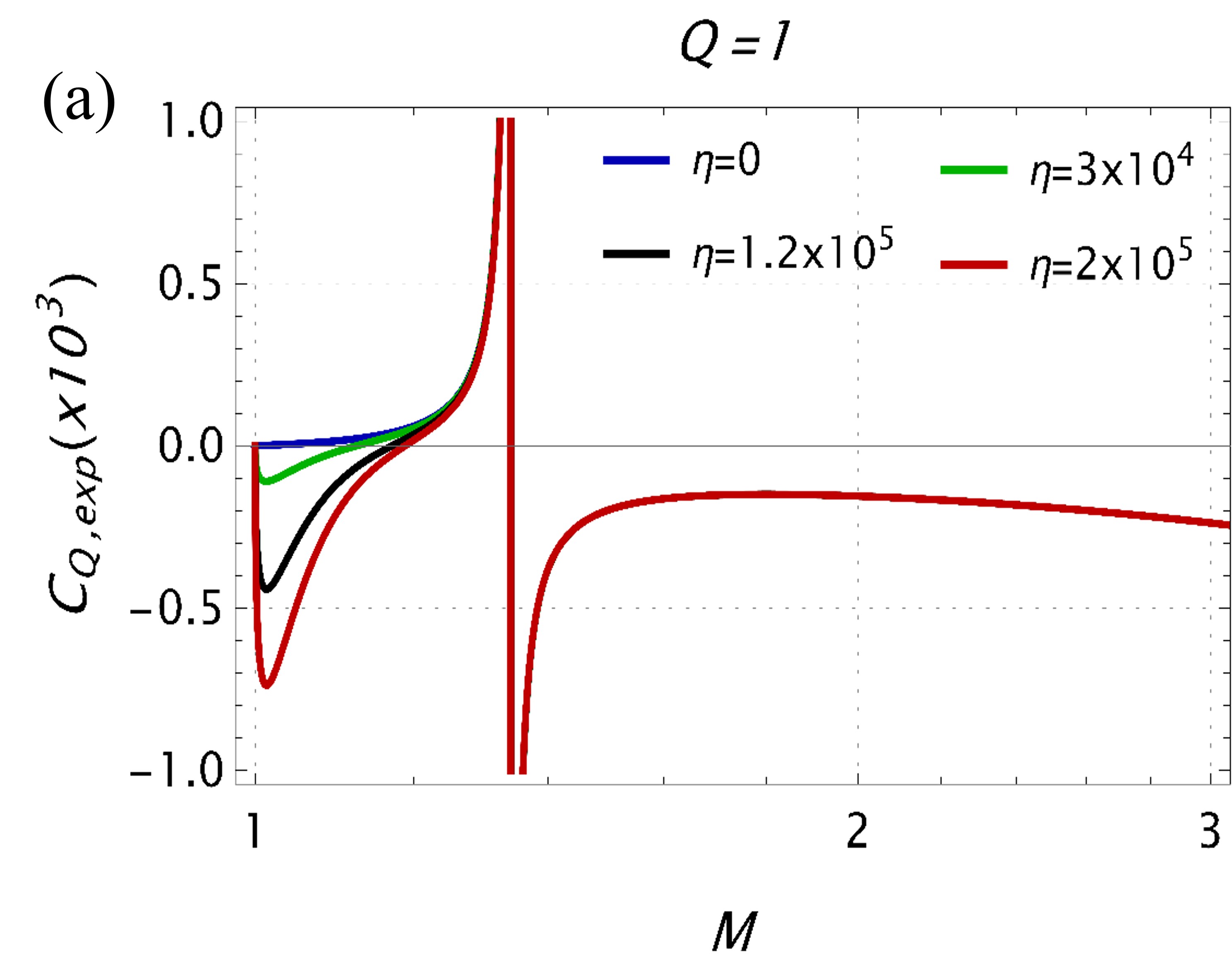
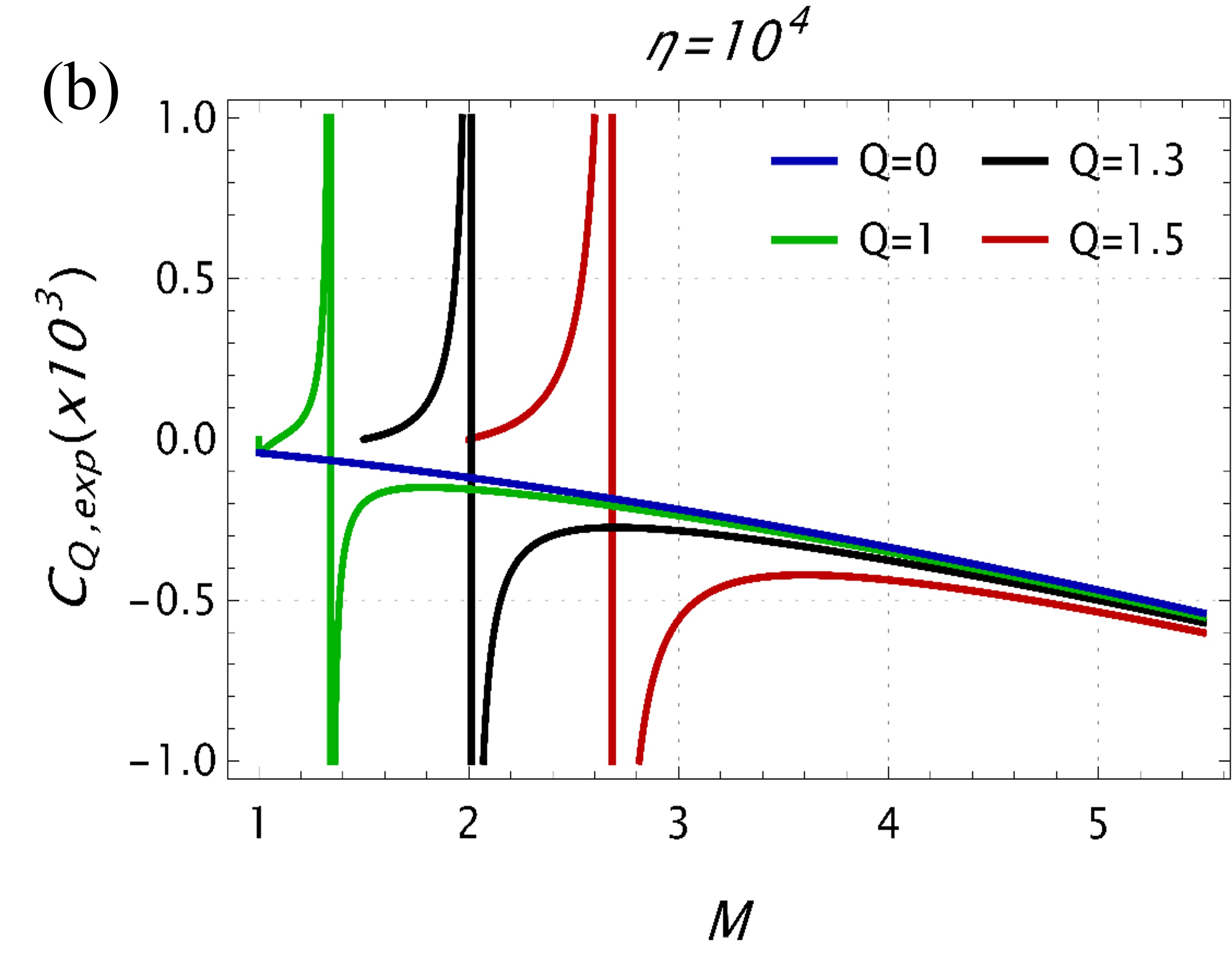
Figure 4: (a) Impact of $\eta$: heat capacity $C_{Q,exp}$ (linear scale) vs BH mass $M$ (log scale), and (b) Impact of charge $Q$ in presence of $\eta$.

The first thing we observe here is that, in both uncorrected ($\eta=0$) and corrected ($\eta\neq 0$) cases, $C_{Q,exp}$ stays negative for larger BH sizes, and suffers from an infinite discontinuity as it shrinks further in size. At this point, it turns from negative to positive, thereby manifesting an unstable to stable phase transition. In particular, this transition represents a second order phase transition. This is somewhat peculiar to charged BHs, conceptualized by Davies 1978RPPh…41.1313D , and is purely of geometric origin due to presence of horizons in the spacetime. Once we enter quantum domain, it then again turns negative through $C_{Q}=0$ in presence of $\eta$, and tends to be more negative (unstable) for larger $\eta$. It finally goes to zero at extremal limit ($M=Q$). This negativity of $C_{Q}$ only occurs in presence of $\eta$, and is absent for $\eta=0$ case. Hence, $\eta$ lends different behaviours to the end stages of our BH as it approaches extremal geometry. $C_{Q}=0$ signifies a first order phase transition. We thus conclude that, with $eta$, our BH always remains thermodynamically in an unstable phase for larger sizes and attains stability for some region before again becoming unstable. So for classical geometries, our BH is unstable, and it undergoes stable/unstable phase transitions in quantum regime. Roots of $C_{Q}$ indicate, what generally are known as bound points, which separate physically acceptable positive temperature solutions from negative (unphysical) ones Hendi:2018sbe . However, in our case, in addition to temperature considerations, it aids in identifying a critical mass $M_{c}$, corresponding to the first root of $C_{Q,exp}$, which marks the onset of phase transitions. We find $M_{c}$ to be

$$M_{c}=\frac{\left(16\log^{8}(\eta)+\pi^{8}Q^{6}\log^{4}(\eta)+\sqrt{\log^{8}(\eta)\left(\pi^{8}Q^{6}-16\log^{4}(\eta)\right)^{2}}\right)^{2/3}+4\pi^{8/3}Q^{2}\log^{4}(\eta)}{4\pi^{4/3}\log^{2}(\eta)\sqrt[3]{16\log^{8}(\eta)+\pi^{8}Q^{6}\log^{4}(\eta)+\sqrt{\log^{8}(\eta)\left(\pi^{8}Q^{6}-16\log^{4}(\eta)\right)^{2}}}},$$ (20)

which obviously depends on $\eta$ and $Q$ on the BH, and this phase transition is absent in original $5$D RNBHs, and has its sole origin in non-perturbative corrections to entropy. Since non-perturbative corrections become relevant only at small (quantum) scales, it is appropriate to treat this as a large (classical) to small (quantum) BH phase transition, quite ubiquitous in BHs Kubiznak:2016qmn . The second zero of heat capacity characterizes a BH that does not exchange energy with its surroundings. This means that the BH ceases evaporation at this stage and ends up as a black remnant. It is hard to ascertain purely from $C_{Q,exp}$ alone what happens beyond this point since our study only concerns up to the extremal limit. As we will see later, thermodynamic geometry conveys much richer structure than heat capacity at extremal limit. This situation finds its parallel in the role of $Q$ as depicted in figure 4 (b). The larger the $Q$, evaporation stops at a larger $M$, $Q$ just quickens the second order phase transition.

It is noteworthy from the right half of the plot in figure 4 (a) that no matter how big the $\eta$ parameter, all plots overlap and become indiscriminate, which depicts that non-perturbative corrections have no role for macroscopic BHs. As a side remark, we juxtapose our thermodynamic observation with the gravitational instabilities of five dimensional Reissner-Nordström BHs. It has been extensively argued that higher dimensional Reissner-Nordström BHs in D$<7$ dimensions generally remain gravitationally stable against large values of $Q$ Kodama:2003ck ; PhysRevLett.103.161101 . However, from thermodynamic point of view, our BH shows an unstable phase for larger sizes as well as smaller sizes. Our findings conform to the arguments presented in Refs. Kodama:2003ck ; PhysRevLett.103.161101 ; Huang:2021jaz for smaller and larger sizes on either side of discontinuity in $C_{Q,exp}$ as seen from figure 4 (b), however, it does not so for larger radii. It would be interesting to take this correlation further, which would perhaps span a separate work.

III.2.2 Logarithmic corrections

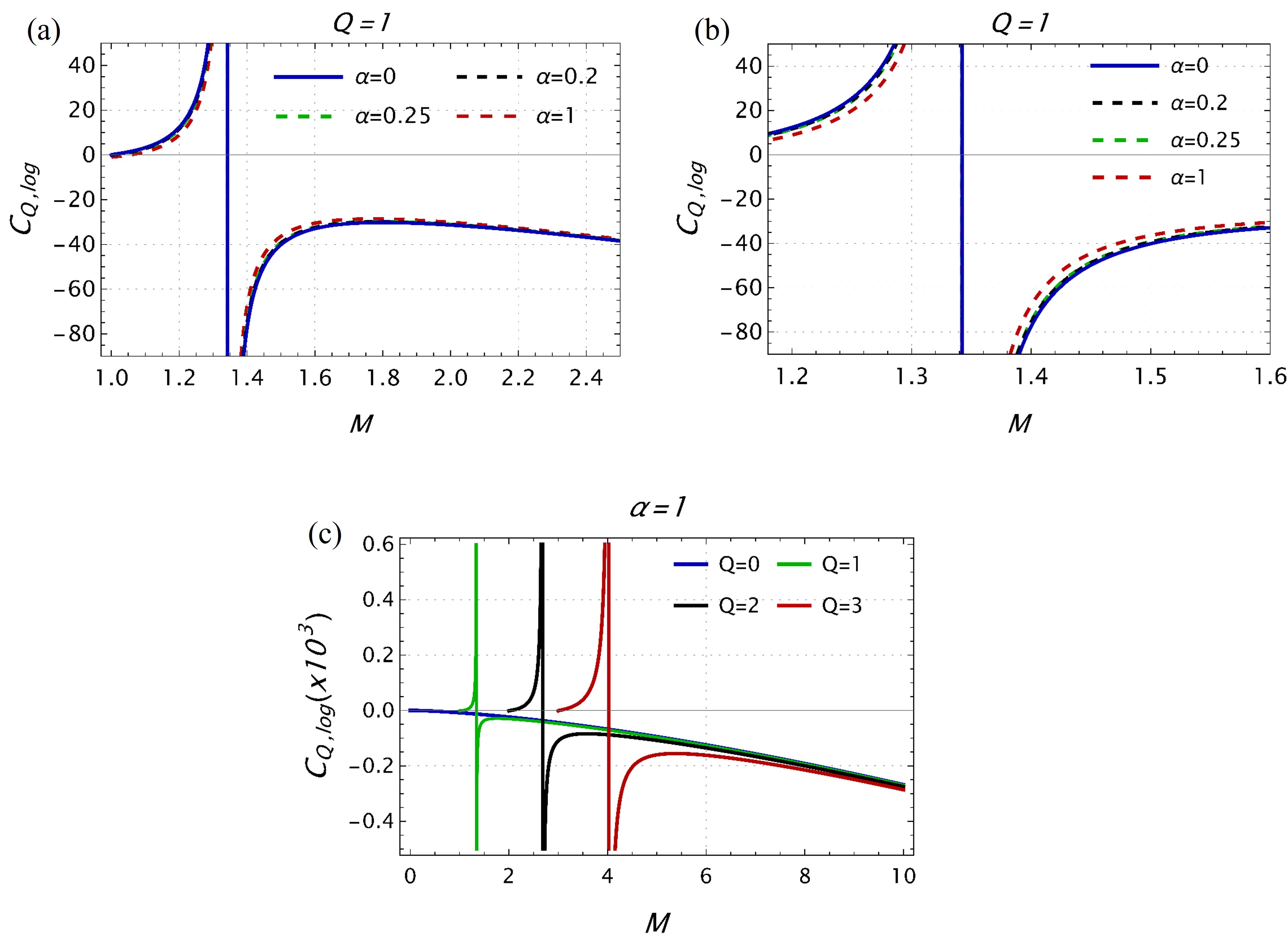
Figure 5: Heat capacity $C_{Q,log}$ variation with mass $M$ for logarithmic corrections: (a) Impact of $\alpha$ for fixed $Q$, (b) zoomed-in view of (a), and (c) Impact of $Q$ for a fixed $\alpha$.

In this case, the heat capacity is given by

$$C_{Q,log} =-\frac{\left(M\left(\sqrt{(M-Q)(M+Q)}+M\right)-Q^{2}\right)}{2\sqrt{(M-Q)(M+Q)}\left(M\left(\sqrt{(M-Q)(M+Q)}+M\right)-3Q^{2}\right)}\Bigg{[}6M^{2}\sqrt{\sqrt{(M-Q)(M+Q)}+M}-4\alpha M-6Q^{2}$$

$$\times\left(\sqrt{\sqrt{(M-Q)(M+Q)}+M}\right)+3\alpha\sqrt{(M-Q)(M+Q)}+6M\sqrt{(M-Q)(M+Q)}\sqrt{\sqrt{(M-Q)(M+Q)}+M}\Bigg{]},$$

and plotted in figure 5.

We observe from figure 5 that for all cases, our BH possesses negative heat capacity $C_{Q,log}$ (unstable) for larger sizes, and a particular behaviour for the case $\alpha$ is only manifested as one approaches extremal limit $(M=Q)$. Uncorrected case $\alpha=0$ (blue line) approaches zero and hence BH remains in stable phase till the remnant forms at $M=Q$. For $\alpha\neq 0$, with fixed $Q$ shown in figure 5 (a), the infinite discontinuity where the system turns from unstable to stable phase and which signifies a second order phase transition, occurs at same value of $M$ for all cases. Hence, in general, our BH is unstable and becomes stable before ending up as remnant at $M=Q$. figure 5 (b) is the close-up view of figure 5 (a), and one can see that for larger values of $\alpha$, heat capacity has increasing trend before the infinite discontinuity, i.e. it tends to make the BH stable. For positive $C_{Q,log}$, after the discontinuity, it lowers heat capacity. Hence it seems thermal fluctuations, embodied in $\alpha$ tend to stabilize BH for large sizes and destabilize it for smaller sizes. The underlying reason may be that for smaller sizes, thermal fluctuations in presence of $\alpha$ make geometry unstable. The infinite discontinuity point is however shifted towards higher $M$ for different values of $Q$ as shown in figure 5 (c), which signifies competition between $M$ and $Q$. Note that unlike exponential case, logarithmic modifications do not have a critical mass in $C_{Q,log}$ inasmuch as it would indicate a large to small BH phase transition. Rather, $C_{Q,log}$ possesses a zero only at $M=Q$, which however represents a remnant. In that sense, the critical mass would correspond to the magnitude of $Q$.

IV Thermodynamic Ruppeiner geometry

Geometric ideas, as enshrined in thermodynamic geometry, have tremendously advanced our understanding of the thermodynamic structure of black holes. A scalar curvature (an invariant) defined in this parameter space helps us to gain further insight into the phase transitions and microscopic structure of black holes. The ideas have been proposed in the context of thermal fluctuation theory, which leads to the thermodynamic Riemannian geometry RevModPhys.67.605 . These so-called information geometric approaches are expected to potentially provide lessons about microscopic degrees of freedom for BHs Ruppeiner:2013yca . To put it simply, if a BH has an associated thermodynamic behaviour just like ordinary gases or fluids, there must be underlying micromolecules with a typical interaction phenomena. We are fortunate enough that information geometry attempts to furnish a deep insight into this microstructure. The first of its kind was formulated by Weinhold doi:10.1063/1.431689 ; doi:10.1063/1.431635 , where a metric defined on the state of equilibrium states with components as Hessian of internal energy. The metric is therefore given by

$$g_{\mu\nu}^{W}=\partial_{\mu}\partial_{\nu}M(S,N^{i}),$$ (21)

where $M$ is internal energy (in geometrized units $c=1$), $S$ is the system’s entropy, and $N^{i}$ constitute all other extensive parameters of system like volume, internal energy etc. $\mu,\nu=0,1,2,..$ are dimensions that correspond to different extensive parameters. This construction gives the following line element

$$ds_{W}^{2}=g_{\mu\nu}^{W}dx^{\mu}dx^{\nu},$$ (22)

from which one can define the curvature scalar (a Gaussian curvature). Inspired by this, Ruppeiner PhysRevA.20.1608 ; RevModPhys.67.605 introduced entropy $S$ in place of $M$ and derived the line element, and it was found that it provides the information about phase transitions. Since then there have been many attempts to extend this information geometric approach to the BH thermodynamics. A Legendre-invariant metric due to Quevedo Quevedo:2006xk ; Quevedo:2008xn attempted to resolve some of issues surrounding Weinhold/Ruppeiner formalism, while a more recent to this row is Hendi-Panahiyan-Eslam-Panah-Momennia (HPEM) metric Hendi:2015rja . Here, we employ the formalism due to Ruppeiner to our BH system as it evaporates to smaller sizes and attempt to reveal the underlying transformation as the hole reduces to quantum scales. Previously, it has been found that all higher-dimensional variants of RNBHs manifest a flat Ruppeiner geometry (zero curvature), thereby indicating an ideal state behaviour Aman:2005xk . However, here we show that the case is not so when the hole size approaches quantum regime dominated by perturbative or non-perturbative quantum corrections. The curvature scalar diverges for exponential case and indicates a phase transition at smaller sizes, which coincides with the zero of $C_{Q,exp}$ (at extremal limit) reported earlier in Section III.

We begin from the well-known Boltzmann entropy relation

$$S=k_{B}\ln\Omega,$$ (23)

where $k_{B}$ is Boltzmann constant and $\Omega$ denotes the number of microstates of system. The inversion of $\Omega$

$$\Omega=\exp{\left(\frac{S}{k_{B}}\right)},$$ (24)

acts as starting point of thermodynamic fluctuation theory from which the Ruppeiner approach emerges. Consider a set of parameters $x^{0}$ and $x^{1}$ which characterize a thermodynamic system (here the BH). The probability of finding this system in the intervals $x^{0}+dx^{0}$ and $x^{1}+dx^{1}$ is given by

$$P(x^{0},x^{1})dx^{0}dx^{1}=\mathcal{A}\Omega(x^{0},x^{1})dx^{0}dx^{1},$$ (25)

where $\mathcal{A}$ is a normalization constant. Upon using eq. (24), we can write

$$P(x^{0},x^{1})\propto\exp{\left(\frac{S}{k_{B}}\right)},$$ (26)

and

$$S(x^{0},x^{1})=S_{bh}(x^{0},x^{1})+S_{E}(x^{0},x^{1}),$$ (27)

where $S_{bh}$ is the BH, $S_{E}$ the environment entropy, such that $S_{bh}<S_{E}\sim S$. For a small change in entropy around equilibrium point $x_{0}^{\mu}$ (where $\mu,\nu=0,1$), we can write the total entropy by expanding it around the equilibrium,

$$S =S_{0}+\frac{\partial S_{bh}}{\partial x^{\mu}}\bigg{|}_{x^{\mu}=x_{0}^{\mu}}\Delta x_{bh}^{\mu}+\frac{\partial S_{E}}{\partial x^{\mu}}\bigg{|}_{x^{\mu}=x_{0}^{\mu}}\Delta x_{E}^{\mu}$$

$$\quad+\frac{1}{2}\frac{\partial^{2}S_{bh}}{\partial x^{\mu}\partial x^{\nu}}\bigg{|}_{x^{\mu}=x_{0}^{\mu}}\Delta x_{bh}^{\mu}\Delta x_{bh}^{\nu}+\frac{1}{2}\frac{\partial^{2}S_{E}}{\partial x^{\mu}\partial x^{\nu}}\bigg{|}_{x^{\mu}=x_{0}^{\mu}}\Delta x_{E}^{\mu}\Delta x_{E}^{\nu}+....,$$

where $S_{0}$ is the equilibrium entropy at $x_{0}^{\mu}$. Now, if one assumes a closed system where extensive parameters of BH and environment $x_{bh}^{\mu}$ and $x_{E}^{\mu}$, respectively, have conservative additive nature, such that $x_{bh}^{\mu}+x_{E}^{\mu}=x_{total}^{\mu}=constant$, then we can write

$$\frac{\partial S_{bh}}{\partial x^{\mu}}\bigg{|}_{x^{\mu}=x_{0}^{\mu}}\Delta x_{bh}^{\mu}=-\frac{\partial S_{E}}{\partial x^{\mu}}\bigg{|}_{x^{\mu}=x_{0}^{\mu}}\Delta x_{E}^{\mu}.$$ (28)

This leads us to

$$\Delta S=\frac{1}{2}\frac{\partial^{2}S_{bh}}{\partial x^{\mu}\partial x^{\nu}}\bigg{|}_{x^{\mu}=x_{0}^{\mu}}\Delta x_{bh}^{\mu}\Delta x_{bh}^{\nu}+\frac{1}{2}\frac{\partial^{2}S_{E}}{\partial x^{\mu}\partial x^{\nu}}\bigg{|}_{x^{\mu}=x_{0}^{\mu}}\Delta x_{E}^{\mu}\Delta x_{E}^{\nu}.$$ (29)

As $S_{E}\sim S$, the second term in eq. (29) is very small and can be ignored, which leaves behind only BH system with the probability given by

$$P(x^{0},x^{1})\propto\exp{\left(-\frac{1}{2}\Delta l^{2}\right)},$$ (30)

where $\Delta l^{2}$ is given by

$$\Delta l^{2}=-\frac{1}{k_{B}}g_{\mu\nu}\Delta x^{\mu}\Delta x^{\nu}.$$ (31)

If we set $k_{B}=1$, we get

$$\Delta l^{2}=g_{\mu\nu}\Delta x^{\mu}\Delta x^{\nu},$$ (32)

where

$$g_{\mu\nu}=-\frac{\partial^{2}S_{bh}}{\partial x^{\mu}\partial x^{\nu}}.$$ (33)

In eq. (32), $\Delta l^{2}$ is a dimensionless, positive definite, invariant quantity, since probability is a scalar quantity. The above line element closely resembles the one in Einstein gravity, and conventionally interpreted as being the thermodynamic length between two equilibrium fluctuation states: thermodynamic states are further apart if the fluctuation probability is less Ruppeiner:2013yca . This is in line with the familiar Le Chatelier’s principle that assures a local thermodynamic stability. The corresponding metric, after dropping the subscript $bh$, reads

$$g_{\mu\nu}=-\frac{\partial^{2}S}{\partial x^{\mu}\partial x^{\nu}},$$ (34)

which is the famous Ruppeiner metric. It is possible to define a curvature scalar for the above line element, similar to what one does in Riemannian geometry. For that matter, consider the Christoffel symbols

$$\Gamma_{\mu\nu}^{\sigma}=\frac{1}{2}g^{\sigma\rho}\left(\partial_{\nu}g_{\rho\mu}+\partial_{\mu}g_{\rho\nu}-\partial_{\rho}g_{\mu\nu}\right),$$ (35)

and the Riemann tensor

$$R_{\rho\mu\nu}^{\sigma}=\partial_{\nu}\Gamma_{\rho\mu}^{\sigma}-\partial_{\mu}\Gamma_{\rho\nu}^{\sigma}+\Gamma_{\rho\mu}^{\delta}\Gamma_{\delta\nu}^{\sigma}-\Gamma_{\rho\nu}^{\delta}\Gamma_{\delta\mu}^{\sigma},$$ (36)

from which we define Ricci tensor and scalar as follows

$$R_{\mu\nu}=R_{\mu\sigma\nu}^{\sigma},\ \ R=g^{\mu\nu}R_{\mu\nu}.$$ (37)

Applying the above method, one can define curvature scalar for Ruppeiner geometry. It turns out that for a $2$-dimensional space with a non-diagonal $g_{\mu\nu}$, Ricci curvature scalar reads Carroll:2004st

$$R =-\frac{1}{\sqrt{g}}\left[\frac{\partial}{\partial x^{0}}\left(\frac{g_{01}}{g_{00}\sqrt{g}}\frac{\partial g_{00}}{\partial x^{1}}-\frac{1}{\sqrt{g}}\frac{\partial g_{11}}{\partial x^{0}}\right)\right.$$ (38)

$$\left.\ \ \ +\frac{\partial}{\partial x^{1}}\left(\frac{2}{\sqrt{g}}\frac{\partial g_{01}}{\partial x^{0}}-\frac{1}{\sqrt{g}}\frac{\partial g_{00}}{\partial x^{1}}-\frac{g_{01}}{g_{00}\sqrt{g}}\frac{\partial g_{00}}{\partial x^{0}}\right)\right],$$ (39)

where $g=\det{g_{\mu\nu}}=g_{00}g_{11}-g_{01}^{2}$. The Ruppeiner metric is

$$g_{\mu\nu}=-\partial_{\mu}\partial_{\nu}S(M,N^{i}),$$ (40)

where $M$ is the BH mass, and $N^{i}$ the set of other extensive parameters. Naturally for our case, we choose charge $Q$ as second extensive variable. The line element therefore reads

$$ds_{R}^{2}=g_{MM}dM^{2}+2g_{MQ}dMdQ+g_{QQ}dQ^{2},$$ (41)

with the metric

$$g_{\mu\nu}=\left({\begin{array}[]{cc}g_{MM}&g_{MQ}\\ g_{QM}&g_{QQ}\\ \end{array}}\right).$$

The components of $g_{\mu\nu}$ are given by

$$g_{MM}=-\frac{\partial}{\partial M}\left(\frac{\partial S}{\partial M}\right),\ g_{MQ}=-\frac{\partial}{\partial M}\left(\frac{\partial S}{\partial Q}\right),$$ (42)

$$g_{QM}=-\frac{\partial}{\partial Q}\left(\frac{\partial S}{\partial M}\right),\ \text{and}\ g_{QQ}=-\frac{\partial}{\partial Q}\left(\frac{\partial S}{\partial Q}\right),$$ (43)

and are detailed in Appendix. Curvature is

$$R =-\frac{1}{\sqrt{g}}\left[\frac{\partial}{\partial M}\left(\frac{g_{MQ}}{g_{MM}\sqrt{g}}\frac{\partial g_{MM}}{\partial Q}-\frac{1}{\sqrt{g}}\frac{\partial g_{QQ}}{\partial M}\right)\right.$$ (44)

$$\left.\ \ \ +\frac{\partial}{\partial Q}\left(\frac{2}{\sqrt{g}}\frac{\partial g_{MQ}}{\partial M}-\frac{1}{\sqrt{g}}\frac{\partial g_{MM}}{\partial Q}-\frac{g_{MQ}}{g_{MM}\sqrt{g}}\frac{\partial g_{MM}}{\partial M}\right)\right],$$ (45)

where $g=\det{g_{\mu\nu}}=g_{MM}g_{QQ}-g_{MQ}^{2}$ (See Appendix).

Before computing Ruppeiner curvature, it is imperative to emphasize the interpretation of it. A zero Ruppeiner curvature has been associated with non-interacting BH molecules- much like an ideal gas. A non-zero Ruppeiner curvature depicts non-vanishing interactions between BH molecules. A negative curvature indicates attractive interactions and vice-versa Ruppeiner:2013yca . If that is the case, a negative curvature would allude to the existence of a stable system. Since Ruppeiner curvature signifies interactions between BH constituents, one would expect a BH system always have a large curvature since it is a collapsed object with incredible density. However, following Ruppeiner’s reasoning Ruppeiner:2013yca , it seems convincing to assume that gravitational degrees of freedom responsible for holding up the system elements might have a non-statistical nature since the gravitating particles have collapsed into central singularity. Thermodynamic curvature merely reflects the interactions (perhaps non-gravitational) among the fluctuating thermodynamic constituents at BH surface originating from the underlying gravity-bound system. In that case, associating an ideal gas-like behaviour with zero curvature makes perfect sense.

IV.1 Exponential corrections

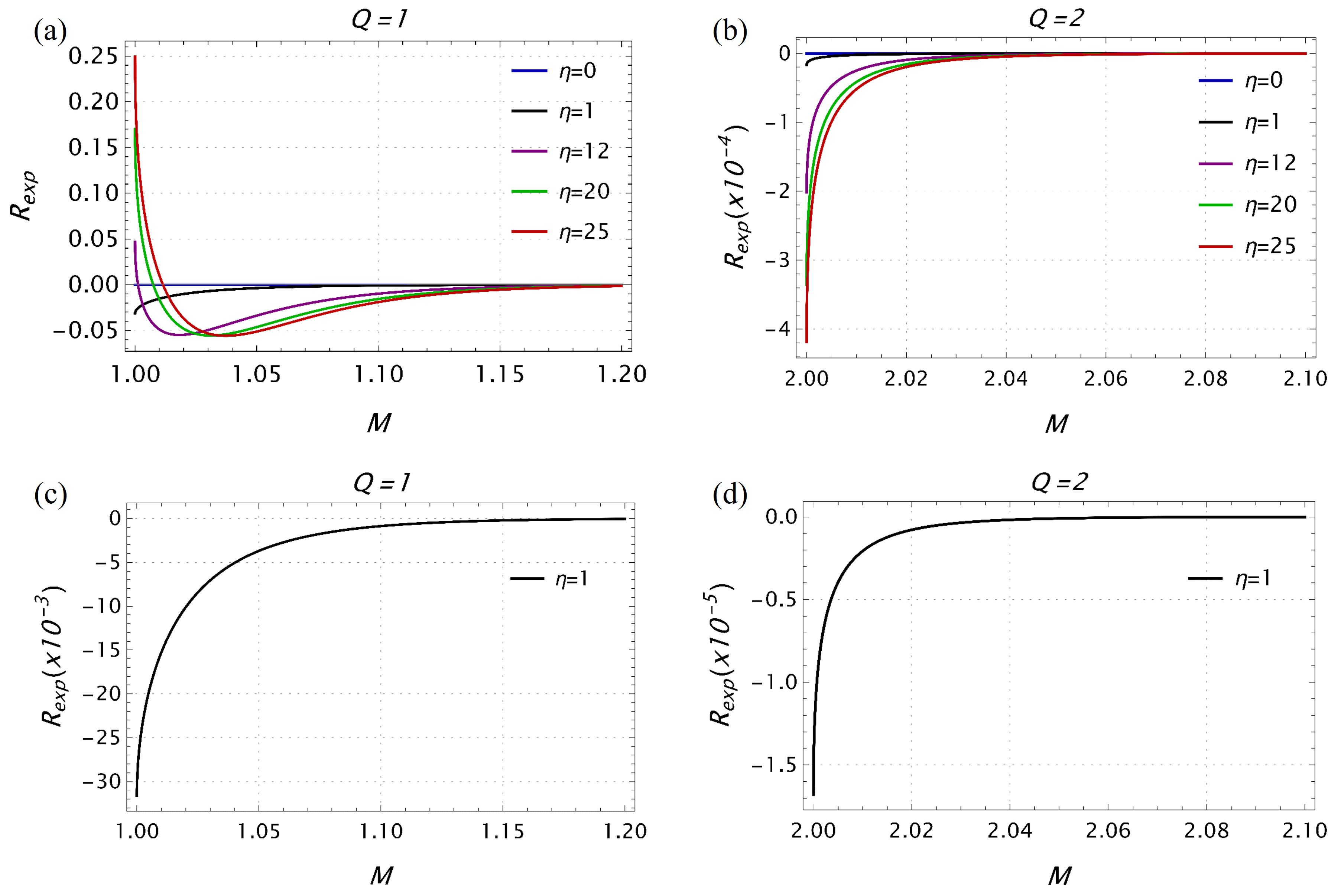
Figure 6: Impact of $\eta$ on Ruppeiner curvature scalar $R_{exp}$ for a fixed $Q$. $R_{exp}$ is zero for bigger hole sizes until $M=Q$, where it diverges and shows a phase transition.

In this section, we discuss thermodynamic geometry of $5$D RNBH in presence of exponential corrections $(\eta)$. Since the final expression for Ruppeiner curvature $R_{exp}$ turns out to be too long, henceforth we only carry out graphical analysis by plotting $R_{exp}$ for a range of parameters. It is possible to plot $R_{exp}$ as a function of mass $M$ while keeping $Q$ fixed. Since for non-extremal case, $M$ exceeds $Q$ which means horizon radii is mostly governed by $M$ than $Q$. We quantify the role of $\eta$ and $Q$ separately. To this end, we present a $2$d plot of $R_{exp}$ for two different values of $Q$ in figure 6.

figure 6 (a) is for $Q=1$ and figure 6 (a) for the case $Q=2$. One can see in both cases, for large sizes with bigger $M$, $R_{exp}$ is zero and changes radically as $M\rightarrow Q$, the quantum domain. Thus our BH manifests a flat geometry for larger sizes and becomes curved (negative or positive) while approaching the extremal limit. This in other words indicates an ideal gas like behaviour for larger sizes, while manifesting multiple phase transitions for smaller (quantum) sizes. At $M=Q$, $R_{exp}\rightarrow\pm\infty$ depending on the choice of $\eta$ and $Q$ signalling a phase transition. First consider the case $Q=1$. As shown in figure 6 (a), for $\eta=1$ (black curve) $\left[\text{see also figure \ref{Rupp2dd} (c) for a clear view}\right]$, $R_{exp}$ diverges to $-\infty$, whilst rest of the cases show positive divergence. Hence we conclude that for $\eta=1$, our BH ends up in a stable phase and unstable for rest of the cases where $R_{exp}\rightarrow+\infty$. $\eta=1$ case possesses only two phase transitions while as rest of the cases have more than two. The first phase transition is where $R_{exp}$ turns from zero to negative, and second one when it goes to positive through zero, before diverging at $M=Q$. So our BH changes from ideal to stable phase, then again ideal phase (momentarily) before becoming unstable. Hence exponential corrections lend a region of stability for the BH before the final phase transition at $M=Q$. Beyond $M=Q$, $R_{exp}$ becomes imaginary and can’t tell anything about the system. For the case $Q=2$, we find all curves behave like $\eta=Q=1$, which means in this case, the BH ends up in a stable phase.

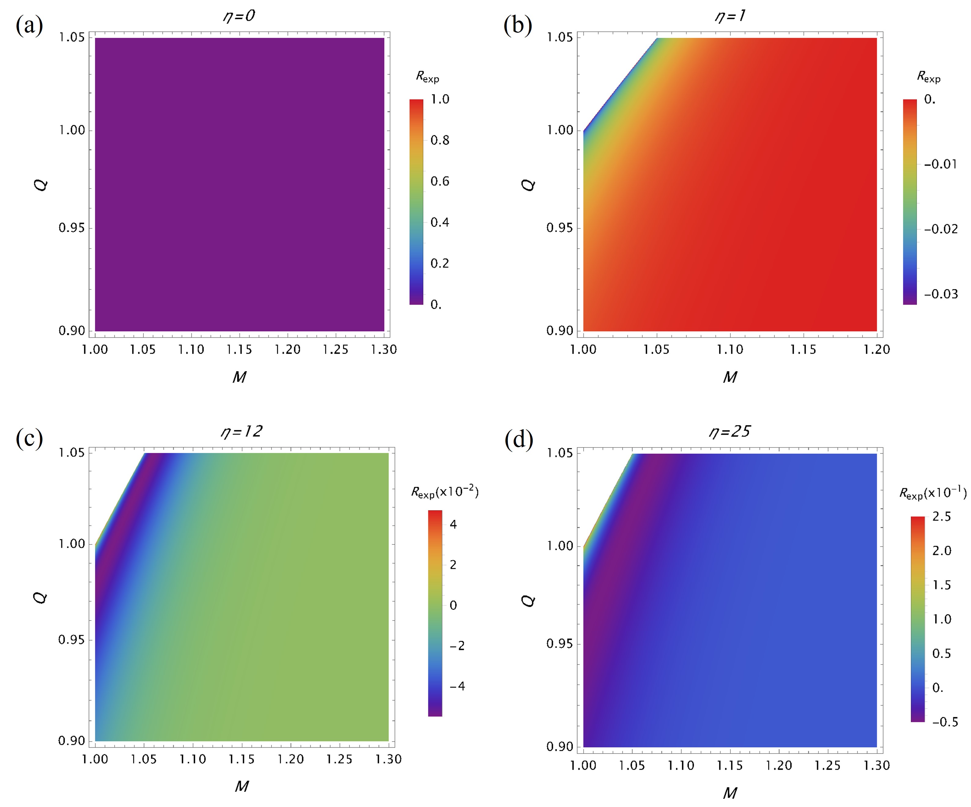
Figure 7: Density plot of $R_{exp}$ to show different regions of stability/instability. Beyond $M=Q$, $R_{exp}$ is imaginary.

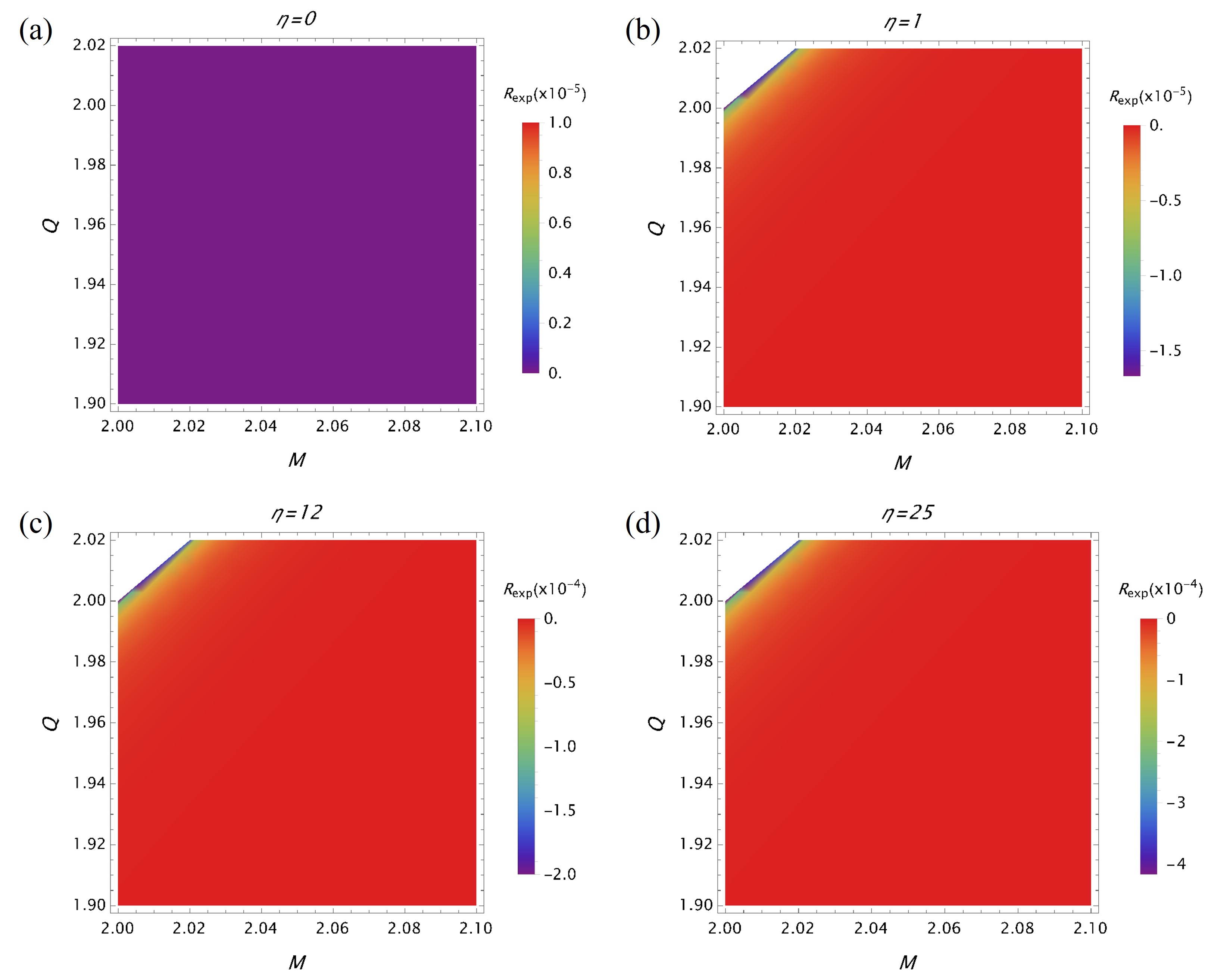
Figure 8: Density plot of $R_{exp}$ to show different regions of stability/instability for the case $Q=2$.

To better appreciate this scenario, we present our results using density plots in figures 7 and 8. One can see that it exactly corroborates the $2$d case as shown above. To be precise, we can see the divergence in $R_{exp}$, beyond which it becomes imaginary. The original unmodified case corresponding to $\eta=0$ [figure 7(a)] for both values of $Q$ shows a flat curvature. It is also important to mention here that divergence points in $R_{exp}$ match with at least one root of $C_{Q,exp}$, i.e. the extremal limit $M=Q$. We also present a parameter space for $R_{exp}$ in figure 9 with respect to $M$ and $\eta$. For classical geometries, $R_{exp}$ is flat, as seen from figure 9 (b), whereas the situation changes in quantum regime, where multiple phase transitions occur [see figure 9 (a)].

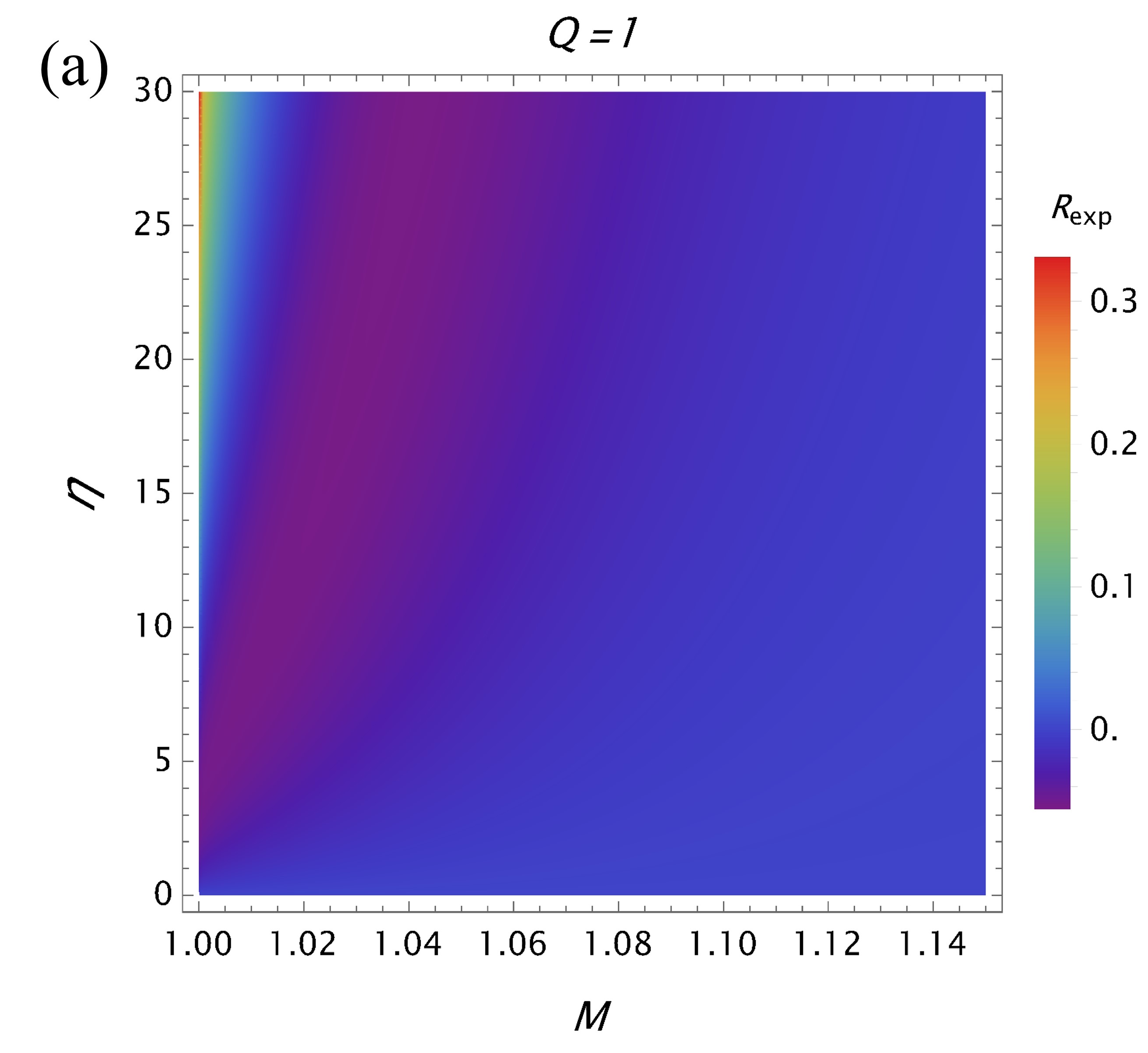
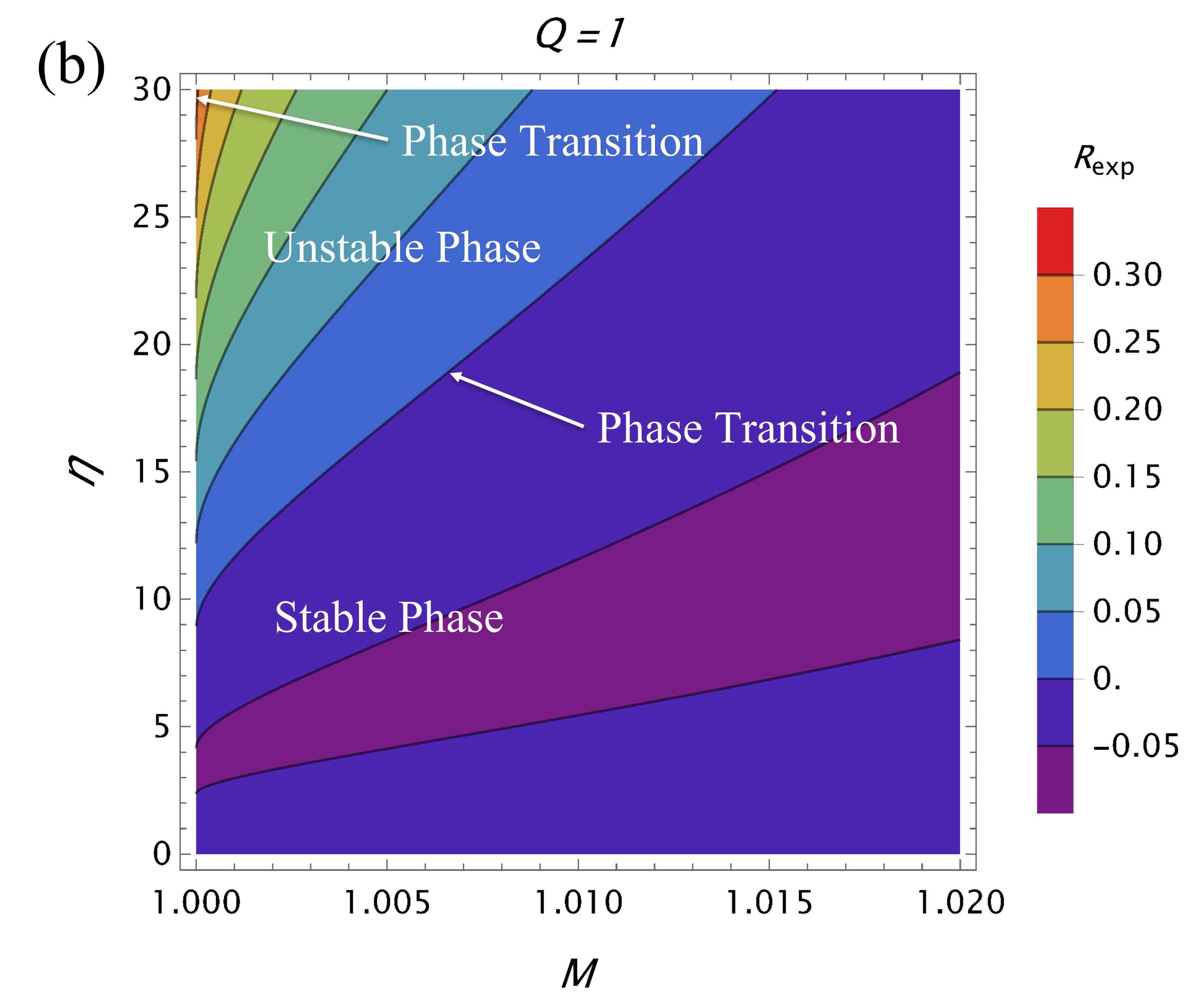
Figure 9: Parameter space of $R_{exp}$ with interplay of $M$ and $\eta$ for fixed $Q$: (a) large BH size view, and (b) small BH size view. Multiple phase transitions can be seen here which arise out of $\eta$.

It has been previously shown in Ref. Aman:2005xk that $5D$ RNBHs possess flat Ruppeiner geometry for all sizes. Our findings show that this holds true for only classical geometries with original Bekenstein-Hawking entropy. Once quantum gravity-inspired entropy is invoked, these results no longer hold for smaller BH sizes, and most importantly, we rather have multiple phase transitions on small scales.

IV.2 Logarithmic corrections

It would be interesting to check the similar physics of Ruppeiner geometry for logarithmic modifications to BH entropy, which as we said earlier are universal in nature though more pronounced on smaller scales. Once again as the expression for curvature turns out to be too long, a graphical analysis would suffice all what we need to unveil.

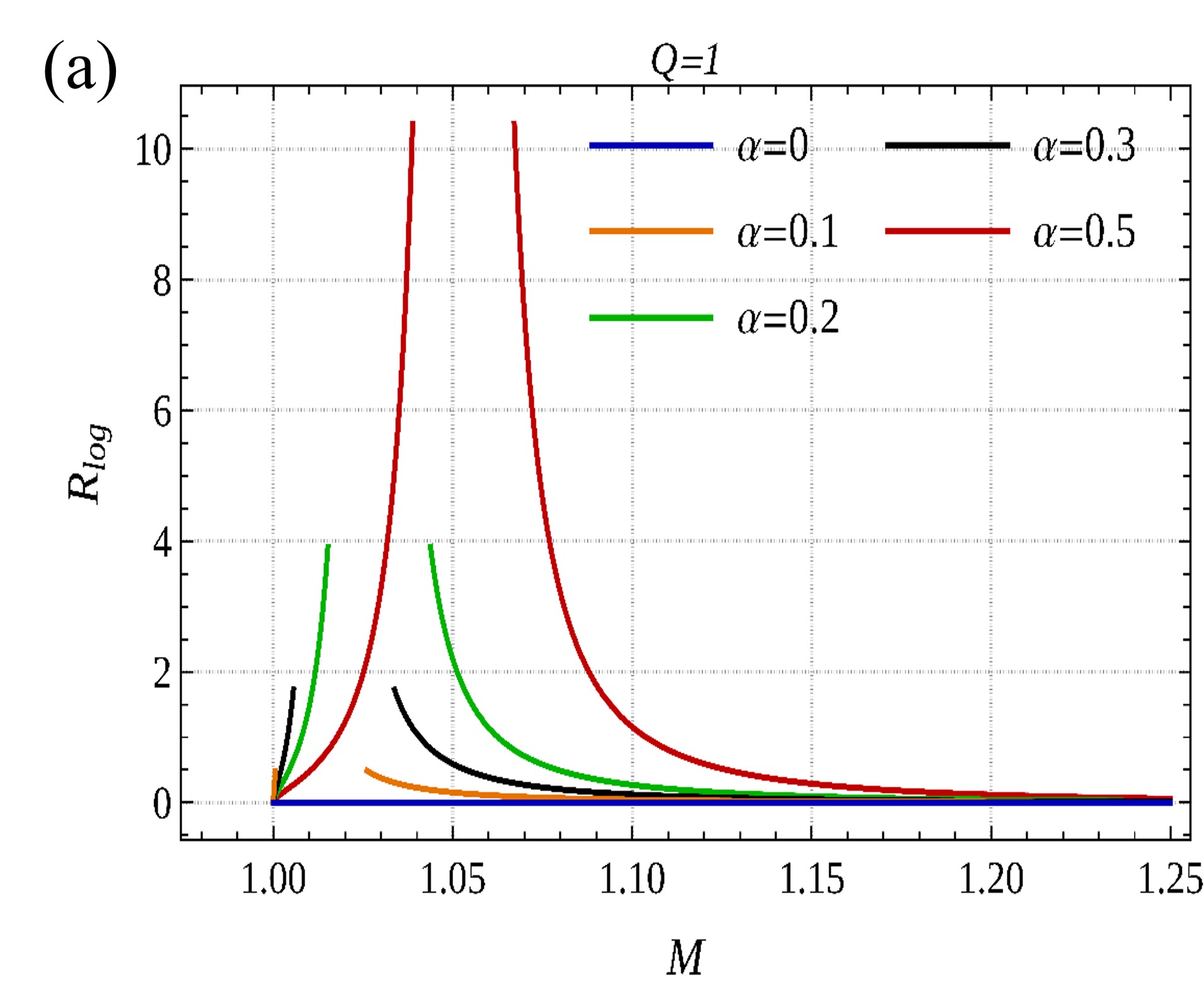
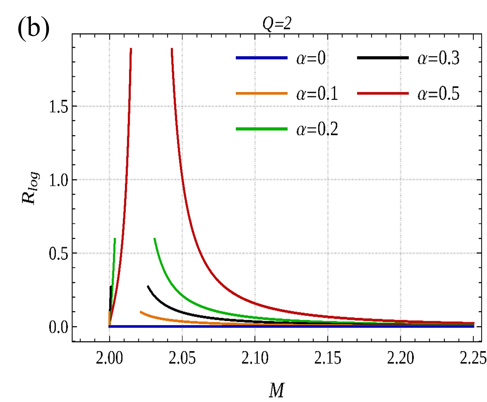
Figure 10: Impact of $\alpha$ on Ruppeiner curvature scalar $R_{log}$.

Similar to exponential case, Ruppeiner geometry is flat $R_{log}=0$ for larger sizes and become positively curved (unstable) as $M$ decreases. There is a positive divergence, $R_{log}\rightarrow+\infty$, indicating a phase transition, before it goes to zero again (ideal phase). The occurrence of divergence in $R_{log}$ depends on magnitude of logarithmic corrections $(\alpha)$, with divergence point shifting towards higher $M$ as $\alpha$ increases. Unlike exponential case, there is no correspondence between divergences in $R_{log}$ and heat capacity divergences or zeros. We conclude, from Ruppeiner geometry analysis, that thermal fluctuations tend to make $5$D RNBH unstable in quantum regime before extremal limit.

V Conclusion

The semi-classical formulation of thermodynamics for BHs rests on the Bekenstein-Hawking entropy, which is inadequate to provide any clues for microscopic origin of thermodynamics. Since at present, we have no sensible theory of quantum gravity, attempts to address this question of mirostructure has ushered us in many directions.

Thermodynamic Ruppeiner geometry is a robust candidate to investigate the microstructure of BHs. A curvature defined on the thermodynamic state space of the system tells us about the underlying interactions among BH constituents. In particular, a positive Ruppeiner curvature shows an unstable system and vice-versa, where as zero curvature indicates an ideal gas-like state.

Here, we used Ruppeiner geometry to uncover the thermodynamic behaviour of an evaporating $5$D RNBH for both classical and quantum domains, when its entropy is modified by non-perturbative (exponential) and perturbative (logarithmic) contributions. Our findings suggest that our BH, under the influence of corrections, may undergo several phase transitions as it approaches extremal limit, where mass and charge balance each other. For exponential corrections, characterized by $\eta$, whether the system is stable or unstable in the region near and at the extremal point solely depends on the choice of $Q$ and $\eta$. The first phase transition occurs around a critical mass scale which differentiates ideal phase from a stable phase ( $R_{exp}=-\text{ve}$ region). $R_{exp}$ finally blows up positively (going via zero) or negatively at extremal limit. For logarithmic modifications quantified by $\alpha$, Ruppeiner curvature $R_{log}$ diverges positively before extremal limit while becoming zero at extremal limit. The divergence point is shifted to larger sizes as $\alpha$ increases.

We emphasize here that, in absence of quantum gravity modifications, the BH manifests zero curvature (Ruppeiner flat), completely agreeing with previous results that show flat Ruppeiner geometry for RNBHs for all higher spacetime dimensions Aman:2005xk .

Appendix : Computing $g_{\mu\nu}$ for Ruppeiner curvature

V.1 Exponential corrections

The components of metric $g_{\mu\nu}$ are given by

$$g_{MM} =\frac{-3\pi^{2}}{16\left(M^{2}-Q^{2}\right)^{3/2}}\Bigg{[}2\sqrt{M+\sqrt{M^{2}-Q^{2}}}\bigg{\{}-3Q^{2}+M\left(M+\sqrt{M^{2}-Q^{2}}\right)\bigg{\}}+\eta e^{-\frac{\pi^{2}}{2}\left(M+\sqrt{M^{2}-Q^{2}}\right)^{3/2}}$$

$$\times\Bigg{\{}12\pi^{2}M^{4}+3\pi^{2}Q^{4}+12\pi M^{3}\sqrt{M^{2}-Q^{2}}+6Q^{2}\sqrt{M+\sqrt{M^{2}-Q^{2}}}-M\sqrt{M^{2}-Q^{2}}$$

$$\times\left(9\pi^{2}Q^{2}+2\sqrt{M+\sqrt{M^{2}-Q^{2}}}\right)-M^{2}\left(15\pi^{2}Q^{2}+2\sqrt{M+\sqrt{M^{2}-Q^{2}}}\right)\Bigg{\}}\Bigg{]},$$

$$g_{MQ} =\frac{-3\pi^{2}Qe^{-\frac{\pi^{2}}{2}\left(M+\sqrt{M^{2}-Q^{2}}\right)^{3/2}}}{16\left(M^{2}-Q^{2}\right)^{3/2}\sqrt{M+\sqrt{M^{2}-Q^{2}}}}\Bigg{[}2e^{\frac{\pi^{2}}{2}\left(M+\sqrt{M^{2}-Q^{2}}\right)^{3/2}}\bigg{\{}-Q^{2}+M\left(M+\sqrt{M^{2}-Q^{2}}\right)\bigg{\}}$$

$$-\eta\Bigg{\{}6\pi^{2}M^{3}\sqrt{M+\sqrt{M^{2}-Q^{2}}}+2M\bigg{(}\sqrt{M^{2}-Q^{2}}-3\pi^{2}Q^{2}\sqrt{M+\sqrt{M^{2}-Q^{2}}}\bigg{)}+Q^{2}\bigg{(}2-3\pi^{2}\sqrt{M^{2}-Q^{2}}$$

$$\times\sqrt{M+\sqrt{M^{2}-Q^{2}}}\bigg{)}+M^{2}\bigg{(}2+6\pi^{2}\sqrt{M^{2}-Q^{2}}\times\sqrt{M+\sqrt{M^{2}-Q^{2}}}\bigg{)}\Bigg{\}}\Bigg{]},$$

$$g_{QM} =\frac{-3\pi^{2}Q}{16\left(M^{2}-Q^{2}\right)^{3/2}}\Bigg{[}2\left(-2M+\sqrt{M^{2}-Q^{2}}\right)\sqrt{M+\sqrt{M^{2}-Q^{2}}}+\eta e^{-\frac{\pi^{2}}{2}\left(M+\sqrt{M^{2}-Q^{2}}\right)^{3/2}}$$

$$\times\Bigg{\{}-6\pi^{2}M^{3}\sqrt{M^{2}-Q^{2}}+M\bigg{(}6\pi^{2}Q^{2}-4\sqrt{M+\sqrt{M^{2}-Q^{2}}}\bigg{)}+\sqrt{M^{2}-Q^{2}}\left(2-3\pi^{2}\sqrt{M^{2}-Q^{2}}\sqrt{M+\sqrt{M^{2}-Q^{2}}}\right)\Bigg{\}}\Bigg{]},$$

$$g_{QQ} =\frac{-3\pi^{2}e^{-\frac{\pi^{2}}{2}\left(M+\sqrt{M^{2}-Q^{2}}\right)^{3/2}}}{16\left(M^{2}-Q^{2}\right)^{3/2}\sqrt{M+\sqrt{M^{2}-Q^{2}}}}\Bigg{[}e^{\frac{\pi^{2}}{2}\left(M+\sqrt{M^{2}-Q^{2}}\right)^{3/2}}\left(-4M^{2}-4M^{2}\sqrt{M^{2}-Q^{2}}+2Q^{2}\sqrt{M^{2}-Q^{2}}\right)$$

$$+\eta\Bigg{\{}4M^{3}-2Q^{2}\sqrt{M^{2}-Q^{2}}-3\pi^{2}Q^{4}\sqrt{M+\sqrt{M^{2}-Q^{2}}}+3\pi^{2}MQ^{2}\sqrt{M^{2}-Q^{2}}\sqrt{M+\sqrt{M^{2}-Q^{2}}}$$

$$+M^{2}\left(4\sqrt{M^{2}-Q^{2}}+3\pi^{2}Q^{2}\sqrt{M+\sqrt{M^{2}-Q^{2}}}\right)\Bigg{\}}\Bigg{]},$$

with the determinant

$$g =\frac{-9\pi^{4}\left(1-\eta e^{-\frac{\pi^{2}}{2}\left(M+\sqrt{M^{2}-Q^{2}}\right)^{3/2}}\right)}{64\left(M^{2}-Q^{2}\right)^{2}\sqrt{M+\sqrt{M^{2}-Q^{2}}}}\Bigg{[}2e^{\frac{\pi^{2}}{2}\left(M+\sqrt{M^{2}-Q^{2}}\right)^{3/2}}\sqrt{M+\sqrt{M^{2}-Q^{2}}}\left(2M^{3}-2MQ^{2}+2M^{2}\sqrt{M^{2}-Q^{2}}-Q^{2}\sqrt{M^{2}-Q^{2}}\right)$$

$$+\eta\Bigg{\{}24\pi^{2}M^{5}+24\pi^{2}M^{4}\sqrt{M^{2}-Q^{2}}+4MQ^{2}\left(3\pi^{2}Q^{2}+\sqrt{M+\sqrt{M^{2}-Q^{2}}}\right)-4M^{2}\sqrt{M^{2}-Q^{2}}$$

$$\times\left(6\pi^{2}Q^{2}+\sqrt{M+\sqrt{M^{2}-Q^{2}}}\right)+Q^{2}\sqrt{M^{2}-Q^{2}}\left(3\pi^{2}+2\sqrt{M+\sqrt{M^{2}-Q^{2}}}\right)\Bigg{\}}\Bigg{]}.$$

V.2 Logarithmic corrections

The metric elements $g_{\mu\nu}$ read as

$$g_{MM} =\frac{1}{4\left(M^{2}-Q^{2}\right)^{2}}\Bigg{[}-M^{2}\left(4\alpha+3\sqrt{M^{2}-Q^{2}}\sqrt{\sqrt{M^{2}-Q^{2}}+M}\right)+3M\left(\alpha\sqrt{M^{2}-Q^{2}}+Q^{2}\sqrt{\sqrt{M^{2}-Q^{2}}+M}\right)$$

$$+Q^{2}\left(9\sqrt{M^{2}-Q^{2}}\sqrt{\sqrt{M^{2}-Q^{2}}+M}-4\alpha\right)-3M^{3}\sqrt{\sqrt{M^{2}-Q^{2}}+M}\Bigg{]},$$

$$g_{MQ} =-\frac{1}{4\left(M^{2}-Q^{2}\right)^{2}}\Bigg{[}Q\Bigg{(}-3M^{2}\sqrt{\sqrt{M^{2}-Q^{2}}+M}+6M\sqrt{(M-Q)(M+Q)}\sqrt{\sqrt{M^{2}-Q^{2}}+M}$$

$$+3Q^{2}\sqrt{\sqrt{M^{2}-Q^{2}}+M}-8\alpha M+3\alpha\sqrt{(M-Q)(M+Q)}\Bigg{)}\Bigg{]},$$

$$g_{QM} =-\frac{1}{4\left(M^{2}-Q^{2}\right)^{2}}\Bigg{[}Q\Bigg{(}-3M^{2}\sqrt{\sqrt{M^{2}-Q^{2}}+M}+6M\sqrt{(M-Q)(M+Q)}\sqrt{\sqrt{M^{2}-Q^{2}}+M}$$

$$+3Q^{2}\sqrt{\sqrt{M^{2}-Q^{2}}+M}-8\alpha M+3\alpha\sqrt{(M-Q)(M+Q)}\Bigg{)}\Bigg{]},$$

$$g_{QQ} =\frac{1}{4\left(Q^{3}-M^{2}Q\right)^{2}}\Bigg{[}3\alpha M^{4}-3M^{3}\Big{(}\alpha\sqrt{M^{2}-Q^{2}}+Q^{2}\sqrt{\sqrt{M^{2}-Q^{2}}+M}\Big{)}+M^{2}Q^{2}\Big{(}9\sqrt{M^{2}-Q^{2}}\sqrt{\sqrt{M^{2}-Q^{2}}+M}-10\alpha\Big{)}$$

$$+3M\Big{(}2\alpha Q^{2}\sqrt{M^{2}-Q^{2}}+Q^{4}\sqrt{\sqrt{M^{2}-Q^{2}}+M}\Big{)}-Q^{4}\Big{(}\alpha+3\sqrt{M^{2}-Q^{2}}\sqrt{\sqrt{M^{2}-Q^{2}}+M}\Big{)}\Bigg{]},$$

with the determinant

$$g =\frac{1}{16\left(Q^{3}-M^{2}Q\right)^{2}}\Bigg{[}-36M^{3}Q^{2}-3M^{2}\left(7\alpha^{2}+12Q^{2}\sqrt{M^{2}-Q^{2}}\right)+\alpha Q^{2}\left(13\alpha-15\sqrt{M^{2}-Q^{2}}\sqrt{\sqrt{M^{2}-Q^{2}}+M}\right)$$

$$+3M\left(7\alpha^{2}\sqrt{M^{2}-Q^{2}}+8\alpha Q^{2}\sqrt{\sqrt{M^{2}-Q^{2}}+M}+12Q^{4}\right)+18Q^{4}\sqrt{M^{2}-Q^{2}}\Bigg{]}.$$

References

- (1) S.-W. Wei and Y.-X. Liu, Insight into the Microscopic Structure of an AdS Black Hole from a Thermodynamical Phase Transition, Phys. Rev. Lett 115 (2015) 111302.
- (2) J.D.Bekenstein, Black Holes and Entropy , Phys. Rev. D 07 (1973) 2333.
- (3) S.W.Hawking, Black hole explosions? , Nature 248 (1974) 30.
- (4) S.W.Hawking, Particle creation by black holes , Comm. Math. Phys. 43 (1975) 199.
- (5) L. Susskind, The world as a hologram , J. Math. Phys. 36 (1995) 6377.
- (6) S.W.Hawking, The Holographic Principle, NATO Sci. Ser. 104 (2003) 75.
- (7) S. Hossenfelder, Minimal Length Scale Scenarios for Quantum Gravity, Living Rev. Rel 16 (2013) 02.
- (8) R. B. Mann and S. N. Soludukhin, Universality of quantum entropy for extreme black holes , Nuc. Phys. B 523 (1995) 293.
- (9) S. Upadhyay, S. H. Hendi, S. Panahiyan, and B. Eslam Panah, Thermal fluctuations of charged black holes in gravity’s rainbow, PTEP 2018 (2013) 093E01.
- (10) B. Pourhassan and S. Upadhyay,Perturbed thermodynamics of charged black hole solution in Rastall theory, Eur. Phys. J. Plus 136 (2013) 311.
- (11) D. Bak and S.-J. Rey, Holographic principle and string cosmology, Class. Quant. Grav. 17 (2000) L1.
- (12) A. Strominger and C. Vafa,Microscopic origin of the Bekenstein-Hawking entropy, Phys. lett. B 379 (1996) 99.
- (13) C. Rovelli,Microscopic origin of the Bekenstein-Hawking entropy, Phys. Rev. Lett. 77 (1996) 3288.
- (14) A. Ashtekar, J. Baez, A. Corichi, and K. Krasnovi, Quantum Geometry and Black Hole Entropy, Phys. Rev. Lett. 80 (1998) 904.
- (15) R. K. Kaul and P. Majumdar , Logarithmic Correction to the Bekenstein-Hawking Entropy , Phys. Rev. Lett. 84 (2000) 5255.
- (16) A. Dabholkar, J. Gomes, and S. Murthy, Counting all dyons in string theory, JHEP 05 (2011) 059.
- (17) I. Mandal and A. Sen, Black Hole Microstate Counting and its Macroscopic Counterpart, Nuclear Physics B - Proceedings Supplements 216 (2011) 147.
- (18) A. Ashtekar, Lectures on Non-Perturbative Canonical Gravity , World Scientific Singapore 06 (1991).
- (19) A. Ghosh and P. Mitra, Absence of log correction in entropy of large black holes, Phys. Lett. B 734 (2014) 49.
- (20) A. Dabholkar, J. Gomes, and S. Murthy, Nonperturbative black hole entropy and Kloosterman sums, JHEP 03 (2015) 074.
- (21) A. Chatterjee and A. Ghosh, Exponential Corrections to Black Hole Entropy , Phys. Rev. Lett. 125 (2020) 041302.
- (22) J. Maldacena, The Large-N Limit of Superconformal Field Theories and Supergravity, Int. J. Theor. Phys 38 (1999) 1113.
- (23) S. Murthy and B. Pioline, A Farey tale for dyons, JHEP 09 (2009) 022.
- (24) A. Dabholkar, J. Gomes, and S. Murthy, Localization & exact holography, JHEP 04 (2013) 062.
- (25) S. Hemming and L. Thorlacius, Thermodynamics of large AdS black holes, JHEP 11 (2007) 086.
- (26) R. Gregory, S. F. Ross, and R. Zegers, Classical and quantum gravity of brane black holes, JHEP 09 (2008) 029.
- (27) J. V. Rochas, Evaporation of large black holes in AdS: coupling to the evaporon, JHEP 08 (2008) 075.
- (28) K. Saraswat and N. Afshordi, Quantum nature of black holes: fast scrambling versus echoes, JHEP 04 (2020) 136.
- (29) A. Sen, Logarithmic corrections to rotating extremal black hole entropy in four and five dimensions, Gen. Rel. Grav. 44 (2012) 1947.
- (30) T. R. Govindarajan, R. K. Kaul, and V. Suneeta, Logarithmic correction to the Bekenstein-Hawking entropy of the BTZ black hole , Class. Quant. Grav. 18 (2001) 2877.
- (31) D. Birmingham and S. Sen, Exact black hole entropy bound in conformal field theory, Phys. Rev. D 63 (2001) 047501.
- (32) B. Pourhassan, M. Faizal, Z. Zaz, and A. Bhat, Quantum fluctuations of a BTZ black hole in massive gravity, Phys. Lett. B 773 (2017) 325.
- (33) B. Pourhassan, S. Upadhyay, H. Saadat, and H. Farahani, Quantum gravity effects on Hořava–Lifshitz black hole, Nuc. Phys. B 928 (2018) 415.
- (34) B. Pourhassan, S. Dey, S. Chougule, and M. Faizal, Quantum corrections to a finite temperature BIon, Class. Quant. Grav. 37 (2020) 135004.
- (35) B. Pourhassan, M. Dehghani, M. Faizal, S. Dey, Non-perturbative quantum corrections to a Born–Infeld black hole and its information geometry, Class. Quant. Grav. 38 (2021) 105001.
- (36) S. Upadhyay, N. ul islam, and P. A. Ganai, A modified thermodynamics of rotating and charged BTZ black hole, JHAP 02 (2022) 25.
- (37) H. Ghaffarnejad and E. Ghasemi, Holographic application in cosmology: Thermodynamics of the Van der Waals cosmic fluid, JHAP 01 (2021) 71.
- (38) M. Biswas, S. Maity, and U. Debnath, Holographic application in cosmology: Thermodynamics of the Van der Waals cosmic fluid, JHAP 01 (2021) 71.
- (39) B. Pourhassan, H. Aounallah, M. Faizal, S. Upadhyay, S. Soroushfar, Y. O. Aitenov, and S. S. Wani, Quantum thermodynamics of an M2-M5 brane system , JHEP 05 (2022) 030.
- (40) B. Pourhassan, M. Atashi, H. Aounallah, S. S. Wani, M. Faizal, and B. Majumder, Quantum thermodynamics of a quantum sized AdS black hole, Nucl.Phys.B 980 (2022) 115842.
- (41) H. Aounallah, H. El Moumni, J. Khalloufi, and K Masmar, Insight into the microscopic structure of a quintessential black hole from the quantization concept, Int. J .Mod. Phys. A 37, 08 (2022), 2250036.
- (42) H. Aounallah, H. Zarei, P. Rudra, B.Majumder, and H. Farahani, P-V Criticality of the Non-linear Charged Black Hole Solutions in Massive Gravity, Preprints (2021), 2021090494. https://doi.org/10.20944/preprints202109.0494.v2.
- (43) T. Jacobson, Thermodynamics of Spacetime: The Einstein Equation of State, Phys. Rev. Lett. 75 (1995) 1260.
- (44) C. Eling, R. Guedens, and T. Jacobson, Nonequilibrium Thermodynamics of Spacetime , Phys. Rev. Lett. 96 (2006) 121301.
- (45) T. Padmanabhan, Thermodynamical aspects of gravity: new insights, Rep. Prog. Phys. 73 (2010) 046901.
- (46) G. Chirco and S. Liberati, Nonequilibrium thermodynamics of spacetime: The role of gravitational dissipation, Rep. Prog. Phys. 81 (2010) 024016.
- (47) R. Guedens, T. Jacobson, and S. Sarkar, Horizon entropy and higher curvature equations of state , Phys. Rev. D 85 (2012) 064017.
- (48) T. Jacobson, Entanglement Equilibrium and the Einstein Equation, Phys. Rev. Lett. 116 (2016) 201101.
- (49) M. Parikh and A. Sveskor, Einstein’s equations from the stretched future light cone , Phys. Rev. Lett. 98 (2018) 026018.
- (50) A. Alonso-Serrano and M. Liška, Quantum phenomenological gravitational dynamics: a general view from thermodynamics of spacetime, JHEP 12 (2020) 196.
- (51) T. Padmanabhan, A Physical Interpretation of Gravitational Field Equations , AIP Conf. Proc. 1241 (2010) 93.
- (52) T. Padmanabhan, Thermodynamical aspects of gravity: new insights, Rept. Prog. Phys. 73 (2010) 046901.
- (53) T. Padmanabhan, Emergent gravity paradigm: Recent progress, Mod. Phys. Lett. A 30 (2015) 153007.
- (54) S. Das, P. Majumdar, and R. K. Bhaduri, General logarithmic corrections to black-hole entropy, Class. Quant. Grav. 19 (2002) 2355.
- (55) M. Faizal, A. Ashour, M. Alcheikh, L. Alasfar, S. Alsaleh, and A. Mahroussah, Quantum fluctuations from thermal fluctuations in Jacobson formalism, Eur. Phys. J. C 77 (2017) 608.
- (56) T. Kaluza, On the Unification Problem in Physics, Int. J. Mod. Phys. D 27 (2018) 14.
- (57) O. Klein, Quantentheorie und fünfdimensionale Relativitätstheorie, Zeitschrift für Physik 37 (1926) 895.
- (58) C. S. Chan, P. L. Paul, and H. L. Verlinde, A note on warped string compactification, Nuc. Phys. B 581 (2000) 156.
- (59) R. Emparan and H. S. Real, Black Holes in Higher Dimensions , Living Rev. Relativ. 11 (2008) 06.
- (60) R. Gregory and R. Laflamme, Black strings and -branes are unstable, Phys. Rev. Lett. 70 (1993) 2837.
- (61) R. Emparan and H. S. Reall, A Rotating Black Ring Solution in Five Dimensions , Phys. Rev. Lett. 88 (2002) 101101.
- (62) R. Emparan, T. Harmark, V. Niarchos, and N. A. Obers, Essentials of blackfold dynamics, JHEP 03 (2010) 063.
- (63) H. Aounallah, B. Pourhassan, S. H. Hendi, and M. Faizal, Five-Dimensional Yang-Mills Black Holes in Massive Gravity’s Rainbow, Eur. Phys. J. C 82 (2022) 351.
- (64) F. R. Tangherlini, Schwarzschild field inn dimensions and the dimensionality of space problem, Nuovo Cim. 27 (1963) 636.
- (65) K. Destounis, Superradiant instability of charged scalar fields in higher-dimensional Reissner-Nordström-de Sitter black holes, Phys. Rev. D 100 (2019) 044054.
- (66) B. Pourhassan and M. Faizal, Quantum corrections to the thermodynamics of black branes, JHEP 10 (2021) 050.
- (67) J. Sadeghi, B. Pourhassan, and M. Rostami,, P-V criticality of logarithm-corrected dyonic charged AdS black holes, JHEP 94 (2016) 064006.
- (68) M. R. R. Good and Y. C. Ong, Particle spectrum of the Reissner–Nordström black hole, Eur. Phys. J. C 80 (2020) 1169.
- (69) S. Mukherji and S. S. Pal, Logarithmic Corrections to Black Hole Entropy and AdS/CFT Correspondence, JHEP 05 (2002) 026.
- (70) J. E. Lidsey, S. Nojiri, S. D. Odintsov, and S. Ogushi, The AdS/CFT correspondence and logarithmic corrections to braneworld cosmology and the Cardy–Verlinde formula, Phys. Lett. B 544 (2002) 337.
- (71) M. H. Dehghani and A. Khoddam-Mohammadi, Thermodynamics of a -dimensional charged rotating black brane and the AdS/CFT correspondence, Phys. Rev. D 67 (2003) 084006.
- (72) S. Das and V. Husain, Anti-de Sitter black holes, perfect fluids and holography, Class. Quant. Grav. 20 (2003) 4387.
- (73) P. Chen, Y. C. Ong, and D.-h. Yeom, Black hole remnants and the information loss paradox, Phys. Rept. 603 (2015) 01.
- (74) P. C. W. Davies, Thermodynamics of black holes, Phys. Rept. 41 (1978) 1313.
- (75) A. Chamblin, R. Emparan, C. V. Johnson, and R. C. Myers, Holography, thermodynamics, and fluctuations of charged AdS black holes, Phys. Rev. D 60 (1999) 104026.
- (76) A. Sheykhi, F. Naeimipour, and S. M. Zebarjad, Phase transition and thermodynamic geometry of topological dilaton black holes in gravitating logarithmic nonlinear electrodynamics, Phys. Rev. D 91 (2015) 124057.
- (77) G. Ruppeiner, Thermodynamic Curvature and Black Holes, Springer Proc. Phys. 153 (2014) 179.
- (78) S. H. Hendi and M. Momennia, AdS charged black holes in Einstein–Yang–Mills gravity’s rainbow: Thermal stability and P-V criticality, Phys. Lett. B 777 (2018) 222.
- (79) D. Kubiznak, R. B. Mann, and M. Teo, Black hole chemistry: thermodynamics with Lambda, Class. Quant. Grav. 34 (2018) 063001.
- (80) H. Kodama and A. Ishibashi, in 7th Hungarian Relativity Workshop (RW 2003), (2003) pp3-18.
- (81) R. A. Konoplya and A. Zhidenko, Instability of Higher-Dimensional Charged Black Holes in the de Sitter World, Phys. Rev. Lett. 103 (2009) 161101.
- (82) J.-H. Huang, R.-D. Zhao, and Y.-F. Zou,, Higher-dimensional non-extremal Reissner-Nordstrom black holes, scalar perturbation and superradiance: An analytical study, Phys. Lett. B 823 (2021) 136724.
- (83) G. Ruppeiner, Riemannian geometry in thermodynamic fluctuation theory, Rev. Mod. Phys. 67 (1995) 605.
- (84) F. Weinhold, Metric geometry of equilibrium thermodynamics, J. Chem. Phys. 63 (1975) 2479.
- (85) F. Weinhold, Metric geometry of equilibrium thermodynamics. II. Scaling, homogeneity, and generalized Gibbs–Duhem relations, J. Chem. Phys. 63 (1975) 2484.
- (86) G. Ruppeiner, Thermodynamics: A Riemannian geometric model, Phys. Rev. A 20 (1979) 1608.
- (87) H. Quevedo, Geometrothermodynamics, J. Math. Phys. 48 (2007) 013506.
- (88) H. Quevedo and A. Sanchez, Geometrothermodynamics of asymptotically Anti-de Sitter black holes, JHEP 09 (2008) 034.
- (89) S. H. Hendi, S. Panahiyan, B. Eslam Panah, and M. Momennia, A new approach toward geometrical concept of black hole thermodynamics, Eur. Phys. J. C 75 (2015) 507.
- (90) J. E. Aman and N. Pidokrajt, Geometry of higher-dimensional black hole thermodynamics, Phys. Rev. D 73 (2006) 024017.
- (91) S. M. Carroll, Spacetime and Geometry , Cambridge University Press (2006).