Abstract

We estimated the spin values of the supermassive black holes (SMBHs) of the active galactic nuclei (AGN) for a large set of Narrow Line Seyfert 1 (NLS1) galaxies assuming the inclination angle between the line of sight and the axis of the accretion disk to be approximately 45 degrees. We found that for these objects the spin values are on average less than for the Seyfert 1 galaxies that we studied previously. In addition, we found that the dependencies of the spin on the bolometric luminosity and the SMBH mass are two to three times stronger that for Seyfert 1 galaxies, which could mean that at early stages of evolution NLS1 galaxies either have a low accretion rate or chaotic accretion, while at later stages they have standard disk accretion, which very effectively increases the spin value.

9 4 175 Academic Editor: Luigi Foschini 17 March 2023 31 March 2023 2 April 2023 3 April 2023 https://doi.org/10.3390/universe9040175 Estimate of SMBH Spin for Narrow-Line Seyfert 1 Galaxies
Accepted for publication in UniverseEstimate of SMBH Spin for Narrow-Line Seyfert 1 Galaxies Mikhail Piotrovich *, Stanislava Buliga and Tinatin Natsvlishvili Mikhail Piotrovich, Stanislava Buliga and Tinatin Natsvlishvili Piotrovich, M.; Buliga, S.; Natsvlishvili, T. Correspondence: mpiotrovich@mail.ru

1 Introduction

There are many types of active galaxies with Active Galactic Nuclei (AGNs), such as Seyfert galaxies, quasars, BL Lac objects, and radio galaxies. Among these types of galaxy, there are two types that are determined by the properties of their emission lines, namely, Seyfert 1 (Sy1) and Seyfert 2 (Sy2) galaxies (Netzer, 2015). Sy1 galaxies exhibit both broad allowed emission lines from the broad line region (BLR) with a width of several thousand km/s, and narrow forbidden emission lines from the narrow line region (NLR) with a width of several hundreds of km/s. Sy2 galaxies are characterized by narrow allowed and forbidden lines in their emission spectra (Robson, 1996). According to the Antonucci (1993) model, both types of galaxies, Sy1 and Sy2, have a similar internal structure, and the differences in their spectra are mainly due to orientation effects. Although the differences between Sy1 and Sy2 galaxies are well defined, galaxies with narrow resolved emission lines, similar to Sy2 galaxies but having all the spectral properties of Sy1 sources, have been found as well. These galaxies have been classified as narrow-line Sy1 (NLS1) galaxies (Osterbrock and Pogge, 1985). Galaxies of this type are characterized by the following: (1) full width at half maximum (FWHM) of the broad line H$\beta$ < 2000 km/s (Goodrich, 1989); (2) weak [OIII] emission lines relative to H$\beta$ with [OIII] $\lambda 5007$/H$\beta$ < 3 (Osterbrock and Pogge, 1985; Leighly, 1999); (3) strong emission lines of FeII relative to H$\beta$ in the ultraviolet and optical regions of the spectrum (Mathur, 2000); (4) a strong excess of soft X-rays and high amplitude of rapid X-ray variability (Boller et al., 1996; Leighly, 1999); (5) strong infrared emissions, indicating active star formation (Moran et al., 1996).

The SMBHs in AGNs are characterized by two main parameters, namely, the mass and the spin (dimensionless angular momentum). The spin is very important because, according to modern concepts, the radiative efficiency of the accretion disk (among other things) strongly depends on the value of the spin (Bardeen et al., 1972; Novikov and Thorne, 1973; Krolik, 2007; Krolik et al., 2007).

In our previous works, we mainly explored AGNs in Seyfert 1-type galaxies; thus, in this work, we decided to study AGNs in NLS1 and to compare these two types of AGNs.

2 Examination of Initial Data

We took initial data from Zhou et al. (2017). This catalogue consists of 2011 NLS1 type objects; of these, 2005 have all the necessary data for our calculations. These include $L_{\text{5100}}$—luminosity at 5100 Å  $FWHM$(H$\beta$)—full width at half maximum of the H$\beta$ spectral line (which determines the rotation speed of an accretion disk of AGN), and $z$—the cosmological redshift.

First, we examine the data from the catalogue. Figures 1–3 show the histograms with the distributions of $L_{\text{5100}}$, $FWHM$(H$\beta$) and the cosmological redshift $z$. We can see that the 5100 Å  that is, the luminosity, has a log-normal distribution with its peak at $\log(L_{\text{5100}}\text{[erg/s]})\approx 44$. Concerning $FWHM$(H$\beta$), it can be seen that the right-hand side of the distribution ends quite abruptly at $\log$($FWHM$(H$\beta$)[km/s]) $\approx 3.4$. This can be explained by the fact that AGNs in NLS1-type objects are characterized by a lower rotation speed of the accretion disk compared to, for example, Seyfert 1 galaxies, as well as by the method used to process the data during the creation of the catalogue (Zhou et al., 2006). The cosmological redshift distribution may be caused by the spatial distribution of objects (for close objects) and the selection effect (for distant objects). Figure 4 shows the dependence of the luminosity at 5100 Å  $L_{\text{5100}}$ on $FWHM$(H$\beta$). The Spearman correlation coefficient for this parameter is 0.28, and the correlation is significant at the 0.05 level. Thus, we can only note a weak correlation between the parameters, which is as expected.

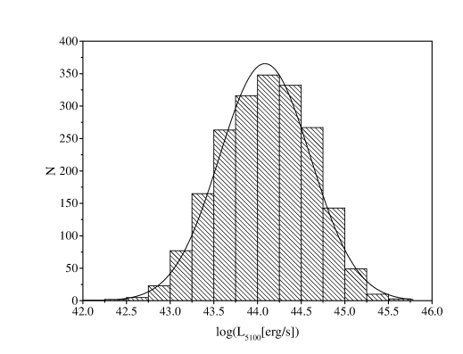
Figure 1: The distribution of the luminosity at 5100 Å  $L_{\text{5100}}$ (with a fitted log-normal distribution curve) from the initial set.

Figure 2: The distribution of $FWHM$(H$\beta$) from the initial set.

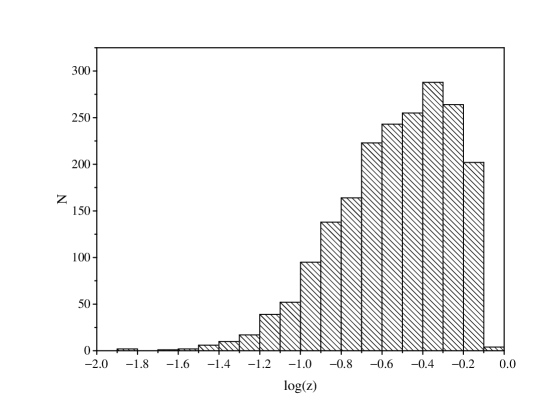
Figure 3: The distribution of the cosmological redshift $z$ from the initial set.

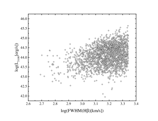
Figure 4: The dependence of $FWHM$(H$\beta$) on the luminosity at 5100 Å  $L_{\text{5100}}$ from the initial set.

3 Estimation of Spin Values

The spin (dimensionless angular momentum) of an SMBH is defined as $a=cJ/GM_{\text{BH}}^{2}$, where $J$ is the angular momentum, $M_{\text{BH}}$ is the mass of the black hole, and $c$ is the speed of light. We can obtain the spin via the radiative efficiency $\varepsilon=L_{\text{bol}}/\dot{M}c^{2}$ (where $L_{\text{bol}}$ is the bolometric luminosity of AGN and $\dot{M}$ is the accretion rate), which depends strongly on the spin of the SMBH (Bardeen et al., 1972; Novikov and Thorne, 1973; Krolik, 2007; Krolik et al., 2007).

There are several models (Davis and Laor, 2011; Raimundo et al., 2012; Du et al., 2014; Trakhtenbrot, 2014; Lawther et al., 2017) connecting the radiative efficiency with the physical parameters of AGNs, which can be obtained from observations. In our previous work (Piotrovich et al., 2022), we concluded that the model from Du et al. (2014) provides the most consistent results; therefore, we decided to use it in this work.

According to Du et al. (2014):

$$\varepsilon\left(a\right)=0.105\left(\frac{L_{\text{bol}}}{10^{46}\,\text{erg/s}}\right)\left(\frac{L_{\text{5100}}}{10^{45}\,\text{erg/s}}\right)^{-1.5}M_{8}\mu^{1.5},$$ (1)

where $M_{8}=M_{\text{BH}}/(10^{8}M_{\odot})$, $\mu=\cos{i}$, and $i$ is the angle between the line of sight and the axis of the accretion disk. Because the angles for most objects are unknown, and because we have no reason to assume the presence of any preferred direction in the orientation of galaxies, the generally accepted method is to assume some average angle. As there is insufficient statistical data on the preferred angle for NLS1, we assume $i=45^{\circ}$, $\mu=0.7$. Although this method is not perfect, there are a number of arguments in its favor; for example, existing angle measurements (including those made with the participation of the authors of the present work (Afanasiev et al., 2018)) show that for most objects of the Seyfert 1 type (including NLS1) they usually range from 20 to 60 degrees, and for a noticeable number of objects the angle is close to 45 degrees (see, for example, Marin (2016); Afanasiev et al. (2018)), which reduces the possible size of errors. Furthermore, in our calculations we use the Eddington ratio $l_{\text{E}}=L_{\text{bol}}/L_{\text{Edd}}$, where $L_{\text{Edd}}=1.3\times 10^{38}M_{\text{BH}}/M_{\odot}$ is the Eddington luminosity.

In order to obtain the bolometric luminosity $L_{\text{bol}}$ from $L_{\text{5100}}$, we need to use bolometric correction. Various authors provide different bolometric corrections that can differ by up to two to three times (Richards et al., 2006; Hopkins et al., 2007; Cheng et al., 2019; Netzer, 2019; Duras et al., 2020). We tested several different methods of bolometric correction, and for consistency decided to use the same method we used in Piotrovich et al. (2022), namely, the approach from Richards et al. (2006): $L_{\text{bol}}=L_{\text{5100}}\times 10.3$.

We obtained the masses of the SMBHs using the method from Vestergaard and Peterson (2006):

$$\log(M_{\text{BH}})\approx\log\left(\left[\frac{FWHM(H\beta)}{1000\,\text{km/s}}\right]^{2}\left[\frac{L_{\text{5100}}}{10^{44}\,\text{erg/s}}\right]^{0.5}\right)+6.91.$$ (2)

The radiative efficiency for this type of object must satisfy the condition $0.039~{}<~{}\varepsilon(a)<0.324$ (Thorne, 1974). In addition, because the method from (Du et al., 2014) uses the Shakura–Sunyaev accretion disk model (Shakura and Sunyaev, 1973), the Eddington ratio must be in the range $0.01\leq l_{\text{E}}\leq 0.3$ (Netzer and Trakhtenbrot, 2014). Thus, from 2005 initial objects, we obtained 474 objects satisfying these conditions. The spin $a$ was determined numerically using the expression from Bardeen et al. (1972):

$$\varepsilon(a)=1-\frac{R_{\text{ISCO}}^{3/2}-2R_{\text{ISCO}}^{1/2}+|a|}{R_{\text{ISCO}}^{3/4}(R_{\text{ISCO}}^{3/2}-3R_{\text{ISCO}}^{1/2}+2|a|)^{1/2}},$$ (3)

where $R_{\text{ISCO}}$ is the radius of the innermost stable circular orbit of the SMBH and

$$\begin{array}[]{l}R_{\text{ISCO}}(a)=3+Z_{2}\pm((3-Z_{1})(3+Z_{1}+2Z_{2}))^{1/2},\\ Z_{1}=1+(1-a^{2})^{1/3}((1+a)^{1/3}+(1-a)^{1/3}),\\ Z_{2}=(3a^{2}+Z_{1}^{2})^{1/2}.\end{array}$$ (4)

In the expression for $R_{\text{ISCO}}(a)$, the sign ”$-$” is used to indicate the prograde ($a\geq 0$), while the sign ”+” indicates the retrograde rotation ($a~{}<~{}0$).

The results of our calculations are presented in Tables 2–15. We must emphasize that the obtained spin values are of course not exact, and can only be considered as estimates intended for statistical analysis. Nevertheless, in the absence of other spin data, they can be used as a first approximation.

4 Analysis of Objects Using Estimated Spin Values

First, we consider the statistical properties of the objects using the estimated spin values (the new set) as compared to the initial set.

Figure 5 shows the distribution of the bolometric luminosity for both sets. It can be seen that both the new set and the initial one have normal distributions; however, in the new set the peak is shifted to the left by an order of magnitude. This can be explained by the fact that we estimated spins only for those objects with Eddington ratios $l_{\text{E}}~{}<~{}0.3$.

Figure 6 demonstrates the distribution of the SMBH mass for both sets. In general, the distributions have a similar form.

Figure 7 shows the distribution of cosmological redshift for both sets. While this distribution again has similar form, its peak is shifted towards closer objects. This occurs because the new set consists of predominantly fainter objects that we are usually only able to detect at closer distances (selection effect).

Figure 8 shows the distribution of the estimated spin values for the 474 objects. The distribution has a pronounced peak at $0.25~{}<~{}a~{}<~{}0.5$ and terminates at $a>0.75$. This is very different from the typical distribution for Seyfert 1-type objects (see Figure 9), for which the distribution usually has its peak at $0.75~{}<~{}a~{}<~{}1.0$ and up to 50% of objects have spin values $a>0.75$ (Trakhtenbrot, 2014; Afanasiev et al., 2018; Piotrovich et al., 2022). This result is generally consistent with the results of Liu et al. (2015) obtained via X-ray observations.

It is interesting to compare our results with the distribution of spins estimated in Chen et al. (2023) (see Figure 6 in their work) for various types of active galaxies. It can be observed that our distribution of spin values for NLS1 looks very similar to their distribution for radio galaxies, which may indicate that these two types of objects are closely related (Yuan et al., 2008; Berton et al., 2018). In addition, it can be seen that our spin distribution for Seyfert 1-type galaxies resembles their distribution for flat-spectrum radio quasars (FSRQ), which in turn could mean that Seyfert 1 galaxies and FSRQs are related (for example, it may mean that these are objects of the same type observed from different directions).

Figure 10 shows the dependence of the estimated spin values $a$ on the bolometric luminosity $L_{\text{bol}}$. The linear fitting provides us with the following expression:

$$a=(0.54\pm 0.05)\log(L_{\text{bol}}\text{[erg/s]})-(23.90\pm 2.05).$$ (5)

In our previous work in Piotrovich et al. (2022), the following was obtained for Seyfert 1 galaxies: $a=(0.25\pm 0.07)\log{L_{\text{bol}}\text{[erg/s]}}-(10.59\pm 3.21)$. Thus, we can conclude that the dependence of the spin on the bolometric luminosity for the NLS1 type is stronger than for Seyfert 1 galaxies.

Figure 11 shows the dependence of the estimated spin values $a$ on the mass of the SMBH $M_{\text{BH}}$. The linear fitting provides us with the following expression:

$$a=(1.25\pm 0.05)\log(M_{\text{BH}}/M_{\odot})-(8.95\pm 0.35).$$ (6)

In Piotrovich et al. (2022), we obtained the following for Seyfert 1 galaxies: $a=(0.46\pm 0.09)\log{M_{\text{BH}}/M_{\odot}}-(3.00\pm 0.71)$. Thus, we can conclude that the dependence of the spin on the SMBH mass is stronger for the NLS1 type than for Seyfert 1 galaxies.

Together with the low average spin, this could mean that at early stages of evolution NLS1 either have low accretion rates or chaotic accretion, while at later stages (which we are studying in this work) they have standard disk accretion, which very effectively increases the spin value.

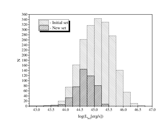
Figure 5: The distribution of the bolometric luminosity for the initial and new sets.

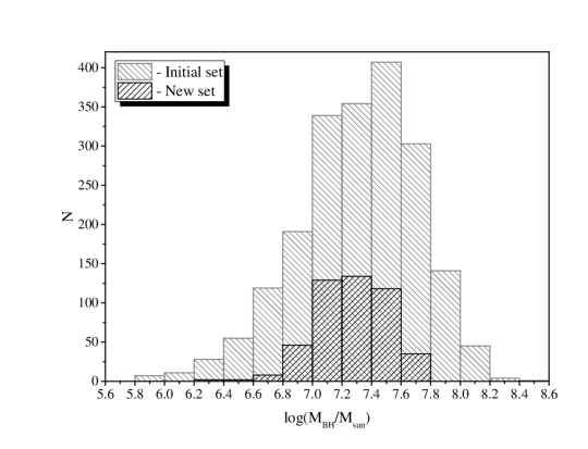
Figure 6: The distribution of the SMBH mass for the initial and new sets.

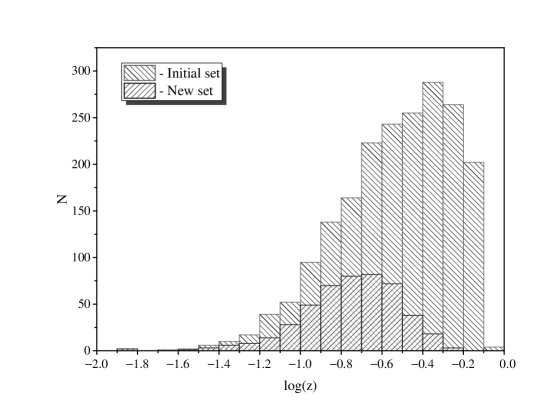
Figure 7: The distribution of the cosmological redshift for the initial and new sets.

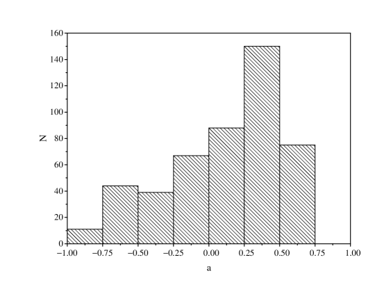
Figure 8: The distribution of the estimated spin values $a$.

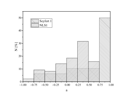
Figure 9: The normalized distributions of the estimated spins for Seyfert 1 (Piotrovich et al., 2022) and NLS1 (this work).

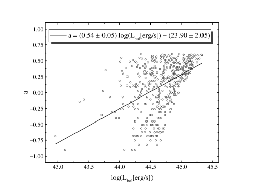
Figure 10: The dependence of the estimated spin values $a$ on the bolometric luminosity $L_{\text{bol}}$.

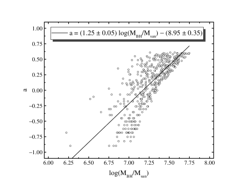
Figure 11: The dependence of the estimated spin values $a$ on the SMBHs masses $M_{\text{BH}}$.

5 Conclusions

In this work, we have estimated spin values of the SMBHs in AGNs for 474 NLS1-type galaxies, assuming the inclination angle between the line of sight and the axis of the accretion disk $i\approx 45^{\circ}$. The distribution of the estimated spin values differs significantly from the distribution of the spins for Seyfert 1-type galaxies. On average, the spin values are smaller. The distribution has a peak at $0.25<a<0.5$, and there are no objects with spins $a>0.75$. This is generally consistent with the results of Liu et al. (2015). Our distribution of spin values for NLS1 looks very similar to the distribution for radio galaxies from Chen et al. (2023), which may indicate that these two types of objects are closely related (Yuan et al., 2008; Berton et al., 2018). In addition, it can be seen that our spin distribution for Seyfert 1-type galaxies in our previous works resembles the distribution from Chen et al. (2023) for flat-spectrum radio quasars (FSRQ), which in turn could mean that Seyfert 1 galaxies and FSRQs are related (for example, it may mean that these are objects of the same type observed from different directions). The dependencies of spin on the bolometric luminosity (Equation (5)) and SMBH mass (Equation (6)) are quite different from the Seyfert 1 case. Specifically, the dependencies of the spin on these parameters is two to three times stronger, which could mean that in the early stages of evolution the NLS1 type either have a low accretion rate or chaotic accretion, while at later stages they have standard disk accretion, which very effectively increases the spin value.

Conceptualization, M.P.; methodology, M.P.; software, M.P.; validation, S.B. and T.N.; formal analysis, M.P.; investigation, M.P., S.B. and T.N.; resources, M.P., S.B. and T.N.; data curation, S.B. and T.N.; writing—original draft preparation, M.P.; writing—review and editing, M.P.; visualization, M.P.; supervision, M.P.; project administration, M.P. All authors have read and agreed to the published version of the manuscript.

This research received no external funding.

Not applicable.

Not applicable.

The data underlying this article are available in the article.

The authors declare no conflict of interest.

no

Appendix A

Table 1: All objects with their estimated spin values. Part 1 of 8. Columns indicate: (1) object name, (2) cosmological redshift, (3) bolometric luminosity, (4) mass of SMBH, and (5) estimated spin value.

Object	$z$	$\log(L_{\text{bol}}\text{[erg/s]})$	$l_{\text{E}}$	$M_{\text{BH}}/M_{\odot}$	$a$
SDSS J000154.27+000732.4	0.139595	44.32	0.126	7.11	0.254
SDSS J001010.03+005126.6	0.387000	45.18	0.293	7.60	0.430
SDSS J001137.24+144201.4	0.131834	44.74	0.165	7.41	0.512
SDSS J001630.43-093853.5	0.239935	45.09	0.269	7.55	0.416
SDSS J002053.31+003812.7	0.144371	44.33	0.135	7.09	0.162
SDSS J002213.00-004832.5	0.213941	44.54	0.195	7.14	$-$0.038
SDSS J002527.35+160226.8	0.110662	44.26	0.131	7.03	0.084
SDSS J002752.39+002615.7	0.205309	44.89	0.245	7.39	0.232
SDSS J002830.95-002402.4	0.167345	44.56	0.147	7.28	0.416
SDSS J002947.82-002258.5	0.228873	44.81	0.228	7.34	0.210
SDSS J003238.20-010035.2	0.091861	44.38	0.147	7.10	0.136
SDSS J003542.67+004735.1	0.148886	44.42	0.183	7.05	$-$0.180
SDSS J003644.72+160830.7	0.465128	45.13	0.259	7.61	0.512
SDSS J003646.45+145936.9	0.089210	44.05	0.125	6.84	$-$0.262
SDSS J003711.00+002127.8	0.235101	44.96	0.235	7.48	0.400
SDSS J003803.51+145057.3	0.138844	44.60	0.282	7.04	$-$0.686

Table 2: Cont.

Object	$z$	$\log(L_{\text{bol}}\text{[erg/s]})$	$l_{\text{E}}$	$M_{\text{BH}}/M_{\odot}$	$a$
SDSS J003846.90+150708.1	0.438353	45.19	0.295	7.61	0.446
SDSS J004241.90+150926.1	0.101278	44.36	0.151	7.07	0.056
SDSS J004742.58-004249.7	0.147298	44.63	0.229	7.16	$-$0.142
SDSS J004809.94+151454.5	0.114583	44.24	0.127	7.03	0.110
SDSS J010009.31+010115.1	0.312451	44.94	0.193	7.54	0.580
SDSS J010044.84+144535.9	0.291464	44.90	0.295	7.32	$-$0.038
SDSS J010407.00+011412.9	0.311880	45.26	0.275	7.71	0.590
SDSS J010546.50+000704.9	0.263738	44.76	0.188	7.38	0.384
SDSS J010950.84+152730.8	0.179014	44.60	0.277	7.05	$-$0.686
SDSS J011009.01-100843.5	0.058116	44.00	0.118	6.82	$-$0.262
SDSS J012801.99+135551.0	0.409060	44.82	0.242	7.33	0.136
SDSS J013521.68-004402.1	0.098500	44.55	0.184	7.17	0.084
SDSS J013556.98+003056.9	0.137892	44.42	0.215	6.98	$-$0.564
SDSS J014019.06-092110.4	0.135279	44.73	0.285	7.17	$-$0.354
SDSS J014105.88-100948.1	0.126420	44.64	0.262	7.11	$-$0.402
SDSS J014153.62+125726.9	0.198901	44.73	0.162	7.41	0.512
SDSS J014248.31-100840.1	0.090390	44.51	0.154	7.21	0.274
SDSS J014248.86+142125.9	0.133879	44.64	0.286	7.07	$-$0.624
SDSS J014559.44+003524.7	0.165335	44.45	0.140	7.19	0.314
SDSS J014951.65+002536.4	0.252437	44.92	0.197	7.52	0.536
SDSS J015046.68+132359.9	0.094126	44.06	0.122	6.87	$-$0.180
SDSS J015219.33+141206.5	0.248238	45.12	0.264	7.59	0.474
SDSS J015313.07-091418.7	0.298273	44.88	0.287	7.31	$-$0.038
SDSS J020132.56+002353.2	0.078002	44.10	0.089	7.04	0.384
SDSS J020844.09+140332.9	0.361032	45.25	0.307	7.65	0.474
SDSS J021529.30-001448.0	0.180980	44.66	0.153	7.37	0.486
SDSS J022008.96-090410.0	0.231675	44.97	0.229	7.50	0.446
SDSS J022226.12-085701.3	0.166732	44.74	0.252	7.23	$-$0.070
SDSS J022347.48-083655.7	0.260775	45.02	0.275	7.47	0.294
SDSS J022821.38-082106.2	0.171374	44.56	0.263	7.03	$-$0.624
SDSS J023038.88-000114.5	0.133688	44.60	0.211	7.16	$-$0.070
SDSS J023315.91-081633.4	0.265553	44.88	0.285	7.31	$-$0.004
SDSS J023414.57+005708.0	0.269222	44.81	0.307	7.21	$-$0.306
SDSS J024225.87-004142.6	0.382742	44.59	0.186	7.21	0.136
SDSS J024546.10-085842.2	0.148299	44.87	0.210	7.44	0.400
SDSS J024621.02+001919.0	0.182892	44.66	0.198	7.25	0.162
SDSS J024727.54-001041.5	0.339179	45.04	0.232	7.57	0.512
SDSS J024934.59-082742.6	0.520684	45.23	0.284	7.67	0.536
SDSS J025416.89-084544.0	0.302060	45.01	0.249	7.50	0.400
SDSS J030639.57+000343.1	0.107344	44.87	0.229	7.40	0.294
SDSS J031532.27+005503.5	0.487399	45.13	0.265	7.60	0.486
SDSS J031722.16-065343.0	0.156204	44.34	0.148	7.06	0.026
SDSS J032801.70+002100.1	0.322078	44.93	0.214	7.49	0.460
SDSS J033502.22-005637.9	0.193281	44.69	0.242	7.20	$-$0.106
SDSS J034131.94-000933.0	0.223370	44.66	0.252	7.15	$-$0.262
SDSS J035827.45-050535.1	0.199733	44.53	0.145	7.26	0.384
SDSS J073606.62+375038.8	0.262155	44.81	0.276	7.26	$-$0.106

Table 3: All objects with their estimated spin values. Part 2 of 8.

Object	$z$	$\log(L_{\text{bol}}\text{[erg/s]})$	$l_{\text{E}}$	$M_{\text{BH}}/M_{\odot}$	$a$
SDSS J073642.77+320915.4	0.184817	44.91	0.224	7.45	0.384
SDSS J074035.86+402234.6	0.177275	44.51	0.234	7.03	$-$0.506
SDSS J074255.78+234252.4	0.336502	44.92	0.266	7.39	0.162
SDSS J074548.27+284838.0	0.158396	44.89	0.283	7.33	0.026
SDSS J074615.57+302400.4	0.206192	44.50	0.169	7.16	0.136

Table 4: Cont.

Object	$z$	$\log(L_{\text{bol}}\text{[erg/s]})$	$l_{\text{E}}$	$M_{\text{BH}}/M_{\odot}$	$a$
SDSS J074906.25+354133.7	0.225995	44.63	0.220	7.18	$-$0.070
SDSS J074940.91+375508.2	0.116532	44.41	0.180	7.04	$-$0.180
SDSS J075141.57+353914.8	0.306203	45.08	0.295	7.50	0.294
SDSS J075209.09+414235.5	0.258357	45.10	0.295	7.52	0.314
SDSS J075347.92+240429.7	0.320213	45.03	0.272	7.49	0.314
SDSS J075433.59+401209.2	0.519061	44.80	0.266	7.26	$-$0.070
SDSS J075525.29+391109.8	0.033513	44.22	0.172	6.87	$-$0.564
SDSS J075606.59+292501.9	0.160578	44.30	0.159	6.99	$-$0.180
SDSS J075613.68+391513.4	0.298794	45.05	0.275	7.50	0.332
SDSS J075616.70+252410.9	0.284962	45.03	0.209	7.60	0.598
SDSS J075659.43+240846.0	0.376471	44.95	0.308	7.35	$-$0.004
SDSS J075838.13+414512.4	0.093531	44.44	0.177	7.08	$-$0.070
SDSS J075922.36+332709.0	0.137888	44.32	0.097	7.22	0.548
SDSS J080135.10+270214.1	0.191474	44.66	0.292	7.08	$-$0.624
SDSS J080203.03+435940.1	0.074398	44.01	0.073	7.04	0.486
SDSS J080252.91+314226.1	0.483675	45.14	0.265	7.61	0.500
SDSS J080416.30+292721.6	0.443993	44.94	0.288	7.37	0.084
SDSS J080439.54+315809.4	0.374000	45.13	0.246	7.63	0.558
SDSS J080515.99+334548.6	0.247069	44.60	0.229	7.13	$-$0.220
SDSS J080538.22+244214.8	0.098837	44.24	0.186	6.86	$-$0.686
SDSS J080710.87+245105.9	0.328634	45.08	0.251	7.57	0.474
SDSS J080742.46+375332.1	0.229941	45.01	0.272	7.47	0.294
SDSS J080807.15+251545.6	0.233955	44.70	0.200	7.29	0.232
SDSS J081231.43+441620.8	0.296883	45.33	0.299	7.74	0.590
SDSS J081252.45+402348.8	0.188447	44.82	0.170	7.48	0.568
SDSS J081321.36+393109.0	0.204989	44.77	0.276	7.22	$-$0.180
SDSS J081345.89+381049.7	0.079960	44.21	0.090	7.15	0.512
SDSS J081422.67+293419.0	0.224970	44.71	0.189	7.32	0.314
SDSS J081427.49+031031.3	0.436499	45.15	0.297	7.57	0.384
SDSS J081427.69+433705.1	0.224183	45.12	0.257	7.60	0.500
SDSS J081503.09+293649.5	0.264458	44.96	0.191	7.57	0.608
SDSS J081516.87+460430.8	0.041184	44.29	0.196	6.89	$-$0.686
SDSS J081823.29+304637.9	0.170442	44.73	0.306	7.13	$-$0.506
SDSS J081835.73+285022.4	0.077240	44.34	0.178	6.98	$-$0.306
SDSS J081836.56+364334.9	0.106051	44.41	0.119	7.22	0.446
SDSS J082050.48+472047.5	0.129067	44.38	0.119	7.19	0.416
SDSS J082405.19+445246.0	0.219632	45.14	0.280	7.58	0.430
SDSS J082432.99+514123.3	0.111106	44.06	0.090	7.00	0.294
SDSS J082447.43+302554.2	0.365092	45.18	0.259	7.66	0.558
SDSS J082921.18+375227.5	0.275902	44.88	0.198	7.47	0.486
SDSS J083013.45+520541.7	0.302577	45.03	0.227	7.56	0.524
SDSS J083052.73+481959.4	0.223419	44.69	0.225	7.23	0.026
SDSS J083105.42+484231.6	0.169707	44.77	0.177	7.41	0.474
SDSS J083202.15+461425.7	0.045906	44.12	0.110	6.97	0.110
SDSS J083225.22+304608.3	0.089738	44.16	0.118	6.98	0.084
SDSS J083237.43+365613.9	0.265764	45.21	0.262	7.68	0.580
SDSS J083352.82+394333.9	0.244864	44.99	0.251	7.48	0.368
SDSS J083454.08+542644.5	0.101118	44.30	0.107	7.16	0.430
SDSS J083651.68+465333.9	0.248637	44.83	0.305	7.24	$-$0.262
SDSS J083810.01+350642.0	0.263217	44.84	0.228	7.37	0.254
SDSS J084000.14+443737.9	0.125391	44.70	0.187	7.32	0.314
SDSS J084314.95+384250.4	0.121095	44.46	0.124	7.26	0.474
SDSS J084818.23+045643.2	0.437673	45.05	0.247	7.55	0.460
SDSS J084855.35+422247.3	0.202080	44.71	0.178	7.35	0.384
SDSS J085026.98+324651.8	0.219877	44.60	0.294	7.02	$-$0.824
SDSS J085039.70+333843.5	0.174862	44.45	0.169	7.11	0.026
SDSS J085256.69+391734.4	0.250059	44.90	0.271	7.36	0.110
SDSS J085315.22+340432.6	0.189949	44.64	0.237	7.16	$-$0.180

Table 5: All objects with their estimated spin values. Part 3 of 8.

Object	$z$	$\log(L_{\text{bol}}\text{[erg/s]})$	$l_{\text{E}}$	$M_{\text{BH}}/M_{\odot}$	$a$
SDSS J085457.23+544820.5	0.255907	45.09	0.268	7.55	0.416
SDSS J085613.17+363144.8	0.171102	44.58	0.207	7.15	$-$0.070
SDSS J085655.29+442653.3	0.179081	44.66	0.144	7.39	0.558
SDSS J085738.56+452513.9	0.242305	44.74	0.176	7.39	0.446
SDSS J085858.79+533917.8	0.242489	44.94	0.232	7.46	0.384
SDSS J090005.80+005835.5	0.250564	44.76	0.233	7.28	0.084
SDSS J090015.28+510800.1	0.126035	44.72	0.202	7.30	0.232
SDSS J090102.33+424957.4	0.213868	44.71	0.262	7.18	$-$0.220
SDSS J090117.82+043656.1	0.319724	45.17	0.306	7.57	0.368
SDSS J090210.16+444625.5	0.266220	45.01	0.247	7.51	0.400
SDSS J090354.72+350959.8	0.241401	44.79	0.262	7.26	$-$0.038
SDSS J090523.95+413107.3	0.494868	44.90	0.207	7.47	0.460
SDSS J090611.61+510928.8	0.097854	44.26	0.126	7.05	0.136
SDSS J090720.90+053833.2	0.383351	45.00	0.278	7.45	0.232
SDSS J090734.53+491911.7	0.141860	44.52	0.122	7.32	0.558
SDSS J090741.40+500814.1	0.208675	44.95	0.255	7.43	0.274
SDSS J090927.69+393229.9	0.152103	44.21	0.177	6.85	$-$0.686
SDSS J091034.21+533725.9	0.187304	44.61	0.182	7.24	0.210
SDSS J091113.39+400111.1	0.200499	44.84	0.291	7.27	$-$0.142
SDSS J091245.77+450046.5	0.318832	44.91	0.199	7.50	0.512
SDSS J091313.72+365817.2	0.107321	44.54	0.185	7.16	0.056
SDSS J091400.03+462937.3	0.136733	44.24	0.189	6.85	$-$0.754
SDSS J091508.55+530310.2	0.248602	45.12	0.234	7.64	0.590
SDSS J091512.23+013412.1	0.455930	44.72	0.199	7.31	0.254
SDSS J091513.89+571233.2	0.195095	44.35	0.198	6.94	$-$0.564
SDSS J091953.24+595128.8	0.215659	44.77	0.189	7.38	0.400
SDSS J092019.52+463608.9	0.155863	44.51	0.253	7.00	$-$0.686
SDSS J092050.41+422408.0	0.174452	44.55	0.254	7.04	$-$0.564
SDSS J092057.50+510700.3	0.200458	44.80	0.177	7.44	0.512
SDSS J092351.17+032231.6	0.179751	44.85	0.292	7.27	$-$0.142
SDSS J092506.70+390708.0	0.247477	44.97	0.283	7.41	0.162
SDSS J092704.38+563351.4	0.219553	44.69	0.141	7.43	0.598
SDSS J092810.50+411129.1	0.152623	44.69	0.145	7.42	0.580
SDSS J093147.74+433119.2	0.132046	44.39	0.132	7.16	0.294
SDSS J093312.47+611936.3	0.122705	44.04	0.086	6.99	0.332
SDSS J093607.86+051034.4	0.207456	44.82	0.259	7.30	0.026
SDSS J093919.90+072755.0	0.409697	45.14	0.308	7.54	0.314
SDSS J094109.86+081404.5	0.125429	44.22	0.148	6.94	$-$0.220
SDSS J094456.07+054642.9	0.212865	44.90	0.290	7.33	$-$0.004
SDSS J094529.36+093610.4	0.013277	43.12	0.055	6.27	$-$0.898
SDSS J094616.90+025459.4	0.117764	44.60	0.192	7.21	0.110
SDSS J094621.26+471131.3	0.230494	45.13	0.289	7.56	0.384
SDSS J094842.67+502931.4	0.056464	44.47	0.162	7.15	0.136
SDSS J094903.55+474653.9	0.214958	44.75	0.252	7.24	$-$0.070
SDSS J095017.60+070317.9	0.108707	44.30	0.175	6.95	$-$0.402
SDSS J095221.96+632438.9	0.119716	44.33	0.115	7.16	0.384
SDSS J095310.69+032725.5	0.184362	44.53	0.125	7.32	0.548
SDSS J095553.14+633742.7	0.356415	45.03	0.238	7.54	0.474
SDSS J095730.15+413301.6	0.318701	45.02	0.255	7.50	0.384
SDSS J095931.67+504449.0	0.143226	45.08	0.300	7.49	0.254
SDSS J100201.77+620816.3	0.133791	44.56	0.226	7.10	$-$0.262
SDSS J100706.25+084228.4	0.373343	45.19	0.300	7.60	0.416
SDSS J100723.15+014546.8	0.355111	44.73	0.266	7.19	$-$0.220
SDSS J100954.65+481514.6	0.178805	44.65	0.169	7.31	0.368
SDSS J101341.90-000925.7	0.277105	44.98	0.267	7.44	0.254
SDSS J101437.45+440639.1	0.200135	45.16	0.270	7.62	0.500

Table 6: Cont.

Object	$z$	$\log(L_{\text{bol}}\text{[erg/s]})$	$l_{\text{E}}$	$M_{\text{BH}}/M_{\odot}$	$a$
SDSS J101549.33+424243.0	0.498800	45.33	0.296	7.75	0.598
SDSS J101645.11+421025.5	0.055322	44.58	0.280	7.02	$-$0.754
SDSS J101852.45+495800.4	0.154811	44.63	0.208	7.20	0.026
SDSS J101936.27+002029.7	0.147878	44.61	0.250	7.10	$-$0.402
SDSS J102000.45+623944.6	0.136020	44.44	0.211	7.01	$-$0.452
SDSS J102049.68+060446.9	0.110954	44.41	0.154	7.11	0.110
SDSS J102148.89+030732.2	0.061838	44.25	0.143	6.98	$-$0.070

Table 7: All objects with their estimated spin values. Part 4 of 8.

Object	$z$	$\log(L_{\text{bol}}\text{[erg/s]})$	$l_{\text{E}}$	$M_{\text{BH}}/M_{\odot}$	$a$
SDSS J102307.02+454500.1	0.256396	44.73	0.166	7.40	0.486
SDSS J102402.59+062943.9	0.044014	43.94	0.117	6.76	$-$0.402
SDSS J102448.57+003538.0	0.095475	44.33	0.154	7.03	$-$0.038
SDSS J102531.28+514034.8	0.044884	44.47	0.242	6.98	$-$0.686
SDSS J102712.37+050320.9	0.338470	44.98	0.280	7.42	0.186
SDSS J102748.92+651337.4	0.444910	44.98	0.279	7.42	0.210
SDSS J102754.27+063107.4	0.159051	44.50	0.217	7.05	$-$0.354
SDSS J102905.51+052555.3	0.122770	44.41	0.132	7.18	0.332
SDSS J102955.38+471346.6	0.175436	44.78	0.218	7.33	0.232
SDSS J103103.52+462616.8	0.093244	44.48	0.171	7.14	0.056
SDSS J104153.59+031500.6	0.093442	44.27	0.099	7.16	0.474
SDSS J104241.08+520012.8	0.136249	44.63	0.242	7.14	$-$0.262
SDSS J104331.50-010732.8	0.361906	45.15	0.274	7.60	0.474
SDSS J104413.32-000324.7	0.279814	45.13	0.291	7.56	0.384
SDSS J104840.49+541302.3	0.104141	44.28	0.194	6.88	$-$0.686
SDSS J105237.41+503042.1	0.245730	45.08	0.259	7.56	0.446
SDSS J110501.99-004454.7	0.332404	45.08	0.238	7.59	0.536
SDSS J110522.54+510727.1	0.307074	45.05	0.288	7.48	0.274
SDSS J110608.03+582609.1	0.118018	44.45	0.217	7.00	$-$0.506
SDSS J110711.32+080538.4	0.281045	45.08	0.233	7.60	0.558
SDSS J110735.68+060758.6	0.380035	45.19	0.290	7.62	0.460
SDSS J111012.07+011327.8	0.094936	45.10	0.302	7.51	0.294
SDSS J111233.81+034007.0	0.321768	44.86	0.223	7.40	0.314
SDSS J111407.35-000031.1	0.072649	44.14	0.136	6.90	$-$0.220
SDSS J111528.48-003454.7	0.232516	44.69	0.199	7.28	0.210
SDSS J111928.85+042655.5	0.153477	44.56	0.167	7.23	0.254
SDSS J111949.75+020256.5	0.207822	44.60	0.221	7.15	$-$0.142
SDSS J112016.16+491428.8	0.149581	44.40	0.208	6.97	$-$0.506
SDSS J112108.58+535121.0	0.102907	45.27	0.298	7.69	0.524
SDSS J112114.22+032546.7	0.152033	45.07	0.267	7.53	0.400
SDSS J112209.40+011719.3	0.058292	44.08	0.164	6.76	$-$0.898
SDSS J112328.12+052823.2	0.101336	44.42	0.145	7.15	0.232
SDSS J112606.43+002349.9	0.169536	44.85	0.169	7.51	0.608
SDSS J112747.17+632542.7	0.341665	44.54	0.209	7.11	$-$0.180
SDSS J112805.72-005850.9	0.284739	45.04	0.226	7.58	0.536
SDSS J112836.17+024550.6	0.238576	44.65	0.168	7.31	0.368
SDSS J113001.88+494434.7	0.244338	45.29	0.301	7.70	0.536
SDSS J113003.11+655629.1	0.132687	44.62	0.276	7.07	$-$0.564
SDSS J113102.27-010122.0	0.242137	44.52	0.256	7.00	$-$0.686
SDSS J113110.64+043856.0	0.144594	44.66	0.184	7.29	0.274
SDSS J113111.94+100231.3	0.074401	44.05	0.112	6.89	$-$0.070
SDSS J113151.04+100915.5	0.119481	44.31	0.213	6.87	$-$0.824
SDSS J113223.43+641958.4	0.209867	45.17	0.261	7.64	0.548

Table 8: Cont.

Object	$z$	$\log(L_{\text{bol}}\text{[erg/s]})$	$l_{\text{E}}$	$M_{\text{BH}}/M_{\odot}$	$a$
SDSS J113229.54+092042.0	0.305157	45.04	0.214	7.60	0.590
SDSS J113320.91+043255.1	0.248058	45.15	0.241	7.66	0.598
SDSS J113842.84-031403.3	0.212339	44.92	0.210	7.49	0.474
SDSS J113900.50+591347.2	0.115052	44.68	0.187	7.30	0.274
SDSS J114203.66+054850.4	0.274033	44.86	0.198	7.45	0.460
SDSS J114208.48+531526.0	0.067965	44.20	0.097	7.10	0.416
SDSS J114341.97-014434.4	0.105223	44.93	0.275	7.38	0.136
SDSS J114514.00+494523.4	0.192336	44.56	0.261	7.03	$-$0.624
SDSS J114632.86+030506.9	0.191294	44.45	0.179	7.09	$-$0.070
SDSS J114928.27-000442.5	0.175967	44.67	0.149	7.39	0.536
SDSS J114958.08+575107.7	0.100556	44.44	0.244	6.94	$-$0.824
SDSS J115050.20+004505.7	0.139474	44.52	0.128	7.30	0.512
SDSS J115215.83+042456.2	0.132674	44.30	0.136	7.06	0.110
SDSS J115655.88+084850.2	0.496092	45.26	0.275	7.71	0.590
SDSS J115713.04+535312.8	0.272882	44.84	0.254	7.32	0.084
SDSS J115715.19+093456.7	0.271835	44.79	0.160	7.48	0.590
SDSS J115723.17+045201.0	0.176083	44.43	0.211	7.00	$-$0.452
SDSS J115741.75+041250.6	0.094812	44.29	0.148	7.01	$-$0.070
SDSS J115755.47+001704.0	0.260770	44.93	0.227	7.46	0.400
SDSS J115852.57+563152.5	0.234345	44.60	0.270	7.06	$-$0.624

Table 9: All objects with their estimated spin values. Part 5 of 8.

Object	$z$	$\log(L_{\text{bol}}\text{[erg/s]})$	$l_{\text{E}}$	$M_{\text{BH}}/M_{\odot}$	$a$
SDSS J115905.80+024802.6	0.168560	44.65	0.216	7.21	$-$0.004
SDSS J120014.08-004638.7	0.179389	44.93	0.236	7.45	0.350
SDSS J120322.36+621505.7	0.270417	44.82	0.303	7.23	$-$0.262
SDSS J120517.71+520109.1	0.189541	44.72	0.210	7.29	0.186
SDSS J120628.97+503001.5	0.171971	44.58	0.272	7.03	$-$0.686
SDSS J121117.80-000212.4	0.181317	44.72	0.177	7.36	0.416
SDSS J121157.48+055801.1	0.067820	44.18	0.136	6.94	$-$0.142
SDSS J121255.27+512221.1	0.282823	44.85	0.241	7.36	0.210
SDSS J121333.20-013220.7	0.197743	44.63	0.204	7.21	0.056
SDSS J121343.76-010002.5	0.328065	44.90	0.239	7.41	0.294
SDSS J121407.35+655228.6	0.235552	45.10	0.238	7.61	0.558
SDSS J121513.83+023334.4	0.224435	44.72	0.157	7.41	0.536
SDSS J121544.73+592639.1	0.095815	44.21	0.122	7.01	0.110
SDSS J121948.93+054531.7	0.113866	44.48	0.166	7.15	0.110
SDSS J122342.82+581446.2	0.014527	42.96	0.042	6.22	$-$0.686
SDSS J122450.55+100545.4	0.167900	44.91	0.244	7.41	0.274
SDSS J122506.20-030100.4	0.239966	44.70	0.297	7.12	$-$0.564
SDSS J122624.42+014020.7	0.219884	44.83	0.176	7.47	0.548
SDSS J122801.33+623948.1	0.271290	44.99	0.251	7.48	0.368
SDSS J122908.95+561109.1	0.265475	44.78	0.180	7.41	0.460
SDSS J122950.61+024652.7	0.336083	45.15	0.284	7.59	0.430
SDSS J123003.50+611904.7	0.148374	44.73	0.276	7.18	$-$0.306
SDSS J123012.17+544719.8	0.276800	44.82	0.201	7.41	0.400
SDSS J123132.52+574624.8	0.259910	44.85	0.218	7.40	0.332
SDSS J123339.58+052034.7	0.215649	44.64	0.226	7.18	$-$0.106
SDSS J123340.07+680022.4	0.343372	44.96	0.244	7.46	0.350
SDSS J123450.50+040845.4	0.121252	44.63	0.244	7.13	$-$0.262
SDSS J123831.33+643456.5	0.101584	44.73	0.221	7.28	0.110
SDSS J124110.10+104143.7	0.156232	44.24	0.168	6.91	$-$0.452
SDSS J124129.34+681533.9	0.150972	44.24	0.128	7.02	0.084
SDSS J124328.04+565237.9	0.106616	44.29	0.165	6.96	$-$0.262

Table 10: Cont.

Object	$z$	$\log(L_{\text{bol}}\text{[erg/s]})$	$l_{\text{E}}$	$M_{\text{BH}}/M_{\odot}$	$a$
SDSS J124504.57+650122.7	0.206591	44.66	0.295	7.08	$-$0.624
SDSS J124504.93+504446.2	0.129684	44.59	0.209	7.16	$-$0.070
SDSS J124519.73-005230.5	0.221020	44.61	0.234	7.13	$-$0.220
SDSS J125051.04+060910.0	0.182047	45.14	0.308	7.54	0.314
SDSS J125156.50+015249.6	0.329416	45.31	0.292	7.73	0.590
SDSS J125224.22+645901.4	0.220729	44.66	0.245	7.16	$-$0.220
SDSS J125227.32+032353.6	0.132687	44.81	0.233	7.33	0.186
SDSS J125248.49+015236.3	0.287988	44.84	0.178	7.48	0.548
SDSS J125357.41+640534.8	0.267455	44.71	0.258	7.19	$-$0.220
SDSS J125635.87+500852.3	0.245337	44.67	0.203	7.25	0.136
SDSS J130030.67+485042.5	0.251725	44.90	0.190	7.51	0.548
SDSS J130052.10+564105.9	0.071838	44.41	0.126	7.20	0.384
SDSS J130421.89+014915.9	0.153597	44.53	0.217	7.08	$-$0.262
SDSS J130547.00+504034.0	0.055124	43.92	0.109	6.77	$-$0.306
SDSS J130717.75+033447.5	0.161346	44.30	0.143	7.03	0.026
SDSS J131136.37+580801.5	0.071088	44.16	0.087	7.11	0.486
SDSS J131234.32+655240.1	0.217351	44.45	0.236	6.97	$-$0.686
SDSS J131305.81+012755.9	0.029361	43.71	0.088	6.65	$-$0.354
SDSS J132026.49+051113.5	0.098391	44.51	0.238	7.02	$-$0.506
SDSS J132231.12-001124.6	0.172930	44.67	0.147	7.39	0.536
SDSS J132428.34+590423.8	0.239623	44.81	0.247	7.31	0.084
SDSS J132447.09+530257.6	0.292005	44.90	0.234	7.42	0.314
SDSS J132640.04+650427.4	0.400867	45.07	0.290	7.50	0.294
SDSS J132704.54-003627.5	0.301717	44.90	0.268	7.36	0.110
SDSS J132705.88-012415.5	0.167808	44.81	0.272	7.26	$-$0.070
SDSS J132731.98+654848.3	0.219769	44.72	0.187	7.34	0.350
SDSS J133059.07+602128.4	0.291747	45.04	0.223	7.58	0.548
SDSS J133138.03+013151.7	0.080473	44.42	0.159	7.11	0.084
SDSS J133248.59+442452.7	0.077438	44.13	0.101	7.02	0.254
SDSS J133315.25+560859.8	0.343105	45.21	0.263	7.68	0.580
SDSS J133328.96+613513.3	0.151516	44.67	0.141	7.41	0.580
SDSS J133627.97+442917.7	0.137809	44.56	0.243	7.06	$-$0.452

Table 11: All objects with their estimated spin values. Part 6 of 8.

Object	$z$	$\log(L_{\text{bol}}\text{[erg/s]})$	$l_{\text{E}}$	$M_{\text{BH}}/M_{\odot}$	$a$
SDSS J133729.04+563907.6	0.143501	44.61	0.213	7.17	$-$0.070
SDSS J134313.40+654110.4	0.240726	44.90	0.231	7.43	0.332
SDSS J134351.06+000434.7	0.073693	44.36	0.104	7.23	0.536
SDSS J134452.91+000520.2	0.087099	44.42	0.124	7.22	0.416
SDSS J134524.69-025939.8	0.085402	44.59	0.156	7.29	0.384
SDSS J134730.70+603742.8	0.143551	44.56	0.146	7.28	0.416
SDSS J135343.63-011801.3	0.145193	44.53	0.168	7.19	0.186
SDSS J135350.63+571725.8	0.234458	44.81	0.274	7.26	$-$0.106
SDSS J135622.94+574150.9	0.309698	44.96	0.292	7.38	0.110
SDSS J135643.69+664128.4	0.172599	44.59	0.257	7.07	$-$0.506
SDSS J135756.53+655902.9	0.197031	44.83	0.284	7.27	$-$0.106
SDSS J135842.27+024925.1	0.148016	44.56	0.170	7.22	0.232
SDSS J135848.54+430435.6	0.252436	44.81	0.242	7.32	0.110
SDSS J135944.07+045649.5	0.085623	44.25	0.169	6.91	$-$0.452
SDSS J140046.05+531920.2	0.388442	45.17	0.285	7.61	0.460
SDSS J140219.69+521059.4	0.279175	44.88	0.271	7.34	0.056
SDSS J140322.10+022232.9	0.250159	44.66	0.308	7.06	$-$0.754
SDSS J140527.68+505546.5	0.106561	44.53	0.153	7.24	0.314
SDSS J140926.77+473127.3	0.143403	44.41	0.220	6.96	$-$0.624

Table 12: Cont.

Object	$z$	$\log(L_{\text{bol}}\text{[erg/s]})$	$l_{\text{E}}$	$M_{\text{BH}}/M_{\odot}$	$a$
SDSS J141108.51+424428.9	0.173315	44.58	0.170	7.24	0.254
SDSS J141419.84+533815.3	0.164455	44.98	0.269	7.44	0.254
SDSS J141424.90+465348.5	0.149731	44.79	0.220	7.34	0.232
SDSS J141820.32-005953.8	0.253638	44.94	0.269	7.40	0.186
SDSS J141838.27+620718.5	0.138792	44.59	0.134	7.35	0.548
SDSS J142103.52+515819.4	0.263543	44.59	0.130	7.37	0.568
SDSS J142214.89+431357.4	0.323267	45.09	0.263	7.56	0.446
SDSS J142509.12+011911.4	0.199814	44.50	0.192	7.11	$-$0.106
SDSS J142542.55+652716.9	0.241476	44.77	0.259	7.25	$-$0.070
SDSS J142830.16+555931.3	0.351431	45.14	0.252	7.63	0.548
SDSS J143030.21-001115.0	0.103284	44.12	0.100	7.01	0.254
SDSS J143223.67+400533.8	0.140651	44.47	0.158	7.16	0.162
SDSS J143249.68+451338.2	0.306872	45.07	0.308	7.47	0.210
SDSS J143407.20+452732.2	0.254952	44.67	0.269	7.13	$-$0.402
SDSS J143601.55+044807.7	0.194125	44.90	0.272	7.36	0.110
SDSS J143704.11+000705.1	0.140363	44.80	0.229	7.33	0.186
SDSS J143715.12+545243.8	0.252154	45.00	0.270	7.46	0.274
SDSS J143952.91+392358.9	0.111999	44.36	0.198	6.95	$-$0.506
SDSS J144013.89-015708.3	0.463581	44.83	0.197	7.43	0.430
SDSS J144205.04+545904.7	0.104628	44.17	0.112	7.01	0.162
SDSS J144237.72+542851.4	0.155188	44.67	0.259	7.15	$-$0.306
SDSS J144249.70+611137.8	0.047858	43.42	0.056	6.56	$-$0.106
SDSS J144328.40+542933.1	0.226942	44.79	0.216	7.35	0.254
SDSS J144507.31+593649.8	0.128030	43.88	0.104	6.75	$-$0.306
SDSS J144705.46+003653.2	0.095493	43.84	0.088	6.78	$-$0.070
SDSS J144920.25+553429.4	0.468295	45.17	0.278	7.62	0.474
SDSS J144945.69+422243.2	0.262760	45.08	0.245	7.58	0.512
SDSS J145123.01-000625.8	0.138613	44.53	0.131	7.30	0.500
SDSS J145201.55+025335.1	0.433702	45.12	0.286	7.55	0.384
SDSS J145235.27+495142.1	0.144921	44.53	0.120	7.34	0.580
SDSS J145624.00+421800.2	0.189834	44.88	0.187	7.50	0.548
SDSS J145643.88+503756.4	0.131486	44.56	0.244	7.06	$-$0.452
SDSS J145801.49+544056.1	0.144858	44.40	0.129	7.18	0.332
SDSS J145921.17+521749.6	0.167019	44.72	0.153	7.43	0.558
SDSS J150034.45+465234.1	0.298022	45.04	0.253	7.53	0.416
SDSS J150238.69+501524.0	0.172268	44.61	0.195	7.21	0.084
SDSS J150346.94+420323.1	0.168316	44.74	0.212	7.30	0.210
SDSS J150816.95+520541.7	0.193395	44.76	0.258	7.24	$-$0.106
SDSS J150832.91+583422.4	0.502172	45.07	0.249	7.56	0.474
SDSS J151020.05+554722.0	0.149693	44.53	0.259	7.01	$-$0.686
SDSS J151024.93+005844.0	0.072262	44.41	0.153	7.11	0.110
SDSS J151101.89+520350.0	0.211340	45.07	0.257	7.55	0.446
SDSS J151131.33+502219.0	0.219845	45.02	0.222	7.56	0.536
SDSS J151616.18+463515.3	0.208271	44.54	0.242	7.05	$-$0.506

Table 13: All objects with their estimated spin values. Part 7 of 8.

Object	$z$	$\log(L_{\text{bol}}\text{[erg/s]})$	$l_{\text{E}}$	$M_{\text{BH}}/M_{\odot}$	$a$
SDSS J151617.16+472805.0	0.197851	44.62	0.227	7.15	$-$0.142
SDSS J151956.57+001614.6	0.114398	44.69	0.257	7.17	$-$0.220
SDSS J152209.56+451124.0	0.065732	44.02	0.098	6.92	0.110
SDSS J152224.45-010838.4	0.321221	45.21	0.257	7.69	0.598
SDSS J152342.49+033147.9	0.221423	44.53	0.235	7.05	$-$0.452
SDSS J152447.13+520759.1	0.160840	44.49	0.214	7.05	$-$0.354
SDSS J152526.40+400914.3	0.355817	45.13	0.256	7.61	0.512
SDSS J152621.69+432349.5	0.155615	44.92	0.270	7.38	0.136

Table 14: Cont.

Object	$z$	$\log(L_{\text{bol}}\text{[erg/s]})$	$l_{\text{E}}$	$M_{\text{BH}}/M_{\odot}$	$a$
SDSS J152628.19-003809.4	0.123334	44.77	0.162	7.45	0.558
SDSS J152840.26+383525.9	0.152598	44.30	0.120	7.11	0.294
SDSS J152843.94+000740.6	0.094440	44.25	0.157	6.94	$-$0.262
SDSS J152912.14+031815.4	0.169956	44.35	0.095	7.26	0.608
SDSS J153006.30+010626.0	0.239339	44.56	0.174	7.21	0.186
SDSS J153252.95+384330.5	0.134003	44.63	0.246	7.13	$-$0.306
SDSS J153458.50+024214.0	0.389458	45.10	0.294	7.52	0.314
SDSS J153607.72+364806.8	0.277578	45.12	0.266	7.59	0.474
SDSS J153651.27+541442.6	0.366706	45.08	0.306	7.48	0.232
SDSS J153705.95+005522.8	0.136419	45.09	0.289	7.52	0.332
SDSS J153937.82+374340.4	0.165048	44.54	0.155	7.24	0.314
SDSS J154113.94+492034.5	0.308087	44.87	0.222	7.41	0.350
SDSS J154623.61+475122.3	0.103287	44.21	0.145	6.94	$-$0.180
SDSS J154656.62+005719.6	0.211019	44.92	0.301	7.33	$-$0.038
SDSS J154814.75+450027.7	0.037268	43.35	0.053	6.52	$-$0.142
SDSS J155427.26+404441.3	0.116805	44.43	0.139	7.18	0.294
SDSS J155451.13+461917.3	0.116881	44.44	0.213	7.00	$-$0.452
SDSS J155637.99+540308.3	0.203331	44.86	0.240	7.37	0.232
SDSS J155755.23+331625.8	0.277693	45.03	0.294	7.45	0.210
SDSS J155851.33+280719.6	0.282557	45.02	0.262	7.49	0.350
SDSS J155904.06+382422.2	0.137065	44.25	0.096	7.16	0.486
SDSS J160344.44+264651.3	0.085673	44.60	0.166	7.27	0.314
SDSS J160404.51+493820.5	0.148582	44.00	0.092	6.93	0.186
SDSS J160426.88+525130.3	0.107031	44.35	0.212	6.91	$-$0.686
SDSS J160558.12+440319.5	0.044438	44.03	0.070	7.07	0.548
SDSS J160806.68+424057.8	0.084737	44.44	0.207	7.01	$-$0.402
SDSS J161527.68+403153.6	0.083355	44.20	0.190	6.81	$-$0.898
SDSS J161713.51+515618.8	0.198799	44.52	0.149	7.24	0.332
SDSS J161951.31+405847.3	0.037858	43.77	0.062	6.87	0.350
SDSS J162755.24+470453.0	0.271820	44.88	0.234	7.40	0.294
SDSS J163128.59+404535.9	0.181227	44.76	0.211	7.32	0.232
SDSS J163152.22+345328.6	0.072234	44.28	0.107	7.14	0.400
SDSS J163214.84+333412.8	0.174118	44.85	0.186	7.47	0.512
SDSS J163247.87+383239.6	0.139247	44.62	0.270	7.08	$-$0.506
SDSS J163417.81+474453.1	0.177306	44.86	0.258	7.34	0.110
SDSS J163625.42+421346.9	0.141250	44.70	0.308	7.10	$-$0.624
SDSS J163737.38+341205.5	0.235658	44.56	0.150	7.27	0.384
SDSS J163927.71+354343.3	0.317929	44.88	0.212	7.44	0.416
SDSS J164100.10+345452.6	0.164078	44.82	0.183	7.45	0.500
SDSS J164207.32+344834.2	0.207533	44.60	0.144	7.33	0.486
SDSS J164225.29+391742.2	0.184353	44.57	0.135	7.33	0.512
SDSS J164416.85+423158.4	0.160893	44.63	0.218	7.18	$-$0.038
SDSS J164626.09+392932.1	0.100365	44.50	0.255	6.98	$-$0.754
SDSS J164907.63+642422.2	0.183524	44.60	0.259	7.08	$-$0.506
SDSS J165437.25+301653.9	0.185698	44.66	0.250	7.15	$-$0.262
SDSS J165636.98+371439.5	0.062757	43.73	0.074	6.75	0.026
SDSS J165658.36+630051.1	0.168969	44.55	0.253	7.04	$-$0.564
SDSS J165757.51+382327.7	0.181496	44.74	0.191	7.35	0.350
SDSS J165914.68+313423.4	0.264525	44.89	0.260	7.37	0.162
SDSS J170002.15+383258.1	0.166573	44.53	0.159	7.22	0.274
SDSS J170546.91+631059.1	0.119182	44.49	0.141	7.23	0.368
SDSS J171033.21+584456.8	0.280701	45.04	0.300	7.45	0.186
SDSS J171526.52+291923.5	0.208273	44.91	0.253	7.40	0.232
SDSS J171540.93+560654.8	0.297139	45.12	0.246	7.62	0.548
SDSS J171943.77+581112.3	0.350752	44.86	0.264	7.33	0.084

Table 15: All objects with their estimated spin values. Part 8 of 8.

Object	$z$	$\log(L_{\text{bol}}\text{[erg/s]})$	$l_{\text{E}}$	$M_{\text{BH}}/M_{\odot}$	$a$
SDSS J204404.53-011214.6	0.172451	44.52	0.223	7.06	$-$0.354
SDSS J204731.68+002056.3	0.181679	44.42	0.126	7.21	0.400
SDSS J205418.80+004915.9	0.227509	45.16	0.243	7.66	0.598
SDSS J210533.44+002829.3	0.054312	43.99	0.124	6.79	$-$0.402
SDSS J210629.86+110109.0	0.304460	45.05	0.287	7.48	0.274
SDSS J211436.68-004938.4	0.145364	44.49	0.148	7.21	0.294
SDSS J212210.99+104200.1	0.299016	44.95	0.232	7.48	0.400
SDSS J212327.26+001439.9	0.182258	44.78	0.277	7.23	$-$0.180
SDSS J213059.76+004438.0	0.130070	44.66	0.292	7.08	$-$0.624
SDSS J213245.28+121256.8	0.125566	44.73	0.149	7.45	0.590
SDSS J214054.55+002538.1	0.083841	44.88	0.308	7.28	$-$0.180
SDSS J214249.64-085434.4	0.135292	44.50	0.162	7.18	0.186
SDSS J214733.86+004021.0	0.124192	44.64	0.277	7.09	$-$0.564
SDSS J215147.60-080922.4	0.120572	44.68	0.204	7.26	0.162
SDSS J220042.72-073056.4	0.110624	44.49	0.243	6.99	$-$0.624
SDSS J220735.12-082457.7	0.213227	44.79	0.277	7.24	$-$0.142
SDSS J221953.18-083258.7	0.305785	44.87	0.282	7.31	$-$0.004
SDSS J222115.58-004030.4	0.171926	44.56	0.137	7.31	0.486
SDSS J222255.55+005033.7	0.112503	44.25	0.199	6.84	$-$0.898
SDSS J224605.44-091925.1	0.118466	44.35	0.154	7.05	$-$0.004
SDSS J225452.22+004631.3	0.090735	44.72	0.308	7.12	$-$0.564
SDSS J230108.39-084848.8	0.171870	44.81	0.199	7.40	0.384
SDSS J230323.47-100235.3	0.180613	44.90	0.285	7.34	0.026
SDSS J230723.24+001708.1	0.112685	44.36	0.209	6.93	$-$0.624
SDSS J231309.71+002633.7	0.285273	44.96	0.261	7.43	0.254
SDSS J233811.52+002045.7	0.278855	44.81	0.198	7.40	0.400
SDSS J234114.22-102828.8	0.277839	44.96	0.219	7.51	0.474
SDSS J234150.81-004329.0	0.250595	44.81	0.260	7.29	$-$0.004
SDSS J234208.30-094747.5	0.191234	44.61	0.210	7.18	$-$0.038
SDSS J234229.45-004731.4	0.315655	44.84	0.269	7.30	$-$0.004
SDSS J234601.30-101549.0	0.191210	44.42	0.113	7.26	0.524
SDSS J234725.29-010643.7	0.182002	44.88	0.236	7.40	0.274
SDSS J235340.46-093709.0	0.311753	44.86	0.227	7.39	0.294

References

yes

References

- Netzer (2015) Netzer, H. Revisiting the Unified Model of Active Galactic Nuclei. Annu. Rev. Astron. Astrophys. 2015, 53, 365–408. [CrossRef]
- Robson (1996) Robson, I. Active Galactic Nuclei; Wiley: New York, NY, USA, 1996.
- Antonucci (1993) Antonucci, R. Unified models for active galactic nuclei and quasars. Annu. Rev. Astron. Astrophys. 1993, 31, 473–521. [CrossRef]
- Osterbrock and Pogge (1985) Osterbrock, D.E.; Pogge, R.W. The spectra of narrow-line Seyfert 1 galaxies. Astrophys. J. 1985, 297, 166–176. [CrossRef]
- Goodrich (1989) Goodrich, R.W. Spectropolarimetry of “Narrow-Line” Seyfert 1 Galaxies. Astrophys. J. 1989, 342, 224. [CrossRef]
- Leighly (1999) Leighly, K.M. A Comprehensive Spectral and Variability Study of Narrow-Line Seyfert 1 Galaxies Observed by ASCA. II. Spectral Analysis and Correlations. Astrophys. J. Suppl. 1999, 125, 317–348.
- Mathur (2000) Mathur, S. Narrow-line Seyfert 1 galaxies and the evolution of galaxies and active galaxies. Mon. Not. R. Astron. Soc. 2000, 314, L17–L20.
- Boller et al. (1996) Boller, T.; Brandt, W.N.; Fink, H. Soft X-ray properties of narrow-line Seyfert 1 galaxies. Astron. Astrophys. 1996, 305, 53.
- Moran et al. (1996) Moran, E.C.; Halpern, J.P.; Helfand, D.J. Classification of IRAS-selected X-ray Galaxies in the ROSAT All-Sky Survey. Astrophys. J. Suppl. 1996, 106, 341. [CrossRef]
- Bardeen et al. (1972) Bardeen, J.M.; Press, W.H.; Teukolsky, S.A. Rotating Black Holes: Locally Nonrotating Frames, Energy Extraction, and Scalar Synchrotron Radiation. Astrophys. J. 1972, 178, 347–370. [CrossRef]
- Novikov and Thorne (1973) Novikov, I.D.; Thorne, K.S. Astrophysics of black holes. In Black Holes (Les Astres Occlus); Dewitt, C., Dewitt, B.S., Eds.; Gordon and Breach: New York, NY, USA, 1973; pp. 343–450.
- Krolik (2007) Krolik, J.H. Making black holes visible: Accretion, radiation, and jets. In Proceedings of the 2007 STScI Spring Symposium on Black Holes, Baltimore, MD, USA, 23–26 April 2007; pp. 309–321.
- Krolik et al. (2007) Krolik, J.H.; Hawley, J.F.; Hirose, S. The Relationship between Accretion Disks and Jets. In Revista Mexicana de Astronomia y Astrofisica; Revista Mexicana de Astronomia y Astrofisica Conference Series; Instituto de Astronomía Distrito Federal: Ciudad de México, Mexico, 2007; Volume 27, pp. 1–7.
- Zhou et al. (2017) Zhou, H.; Wang, T.; Yuan, W.; Lu, H.; Dong, X.; Wang, J.; Lu, Y. VizieR Online Data Catalog: Narrow line Seyfert 1 galaxies from SDSS-DR3 (Zhou+, 2006). VizieR Online Data Cat. 2017. [CrossRef]
- Zhou et al. (2006) Zhou, H.; Wang, T.; Yuan, W.; Lu, H.; Dong, X.; Wang, J.; Lu, Y. A Comprehensive Study of 2000 Narrow Line Seyfert 1 Galaxies from the Sloan Digital Sky Survey. I. The Sample. Astrophys. J. Suppl. 2006, 166, 128–153.
- Davis and Laor (2011) Davis, S.W.; Laor, A. The Radiative Efficiency of Accretion Flows in Individual Active Galactic Nuclei. Astrophys. J. 2011, 728, 98.
- Raimundo et al. (2012) Raimundo, S.I.; Fabian, A.C.; Vasudevan, R.V.; Gandhi, P.; Wu, J. Can we measure the accretion efficiency of active galactic nuclei? Mon. Not. R. Astron. Soc. 2012, 419, 2529–2544.
- Du et al. (2014) Du, P.; Hu, C.; Lu, K.X.; Wang, F.; Qiu, J.; Li, Y.R.; Bai, J.M.; Kaspi, S.; Netzer, H.; Wang, J.M.; et al. Supermassive Black Holes with High Accretion Rates in Active Galactic Nuclei. I. First Results from a New Reverberation Mapping Campaign. Astrophys. J. 2014, 782, 45.
- Trakhtenbrot (2014) Trakhtenbrot, B. The Most Massive Active Black Holes at z 1.5–3.5 have High Spins and Radiative Efficiencies. Astrophys. J. Lett. 2014, 789, L9.
- Lawther et al. (2017) Lawther, D.; Vestergaard, M.; Raimundo, S.; Grupe, D. A catalogue of optical to X-ray spectral energy distributions of z 2 quasars observed with Swift—I. First results. Mon. Not. R. Astron. Soc. 2017, 467, 4674–4710.
- Piotrovich et al. (2022) Piotrovich, M.Y.; Buliga, S.D.; Natsvlishvili, T.M. Determination of supermassive black hole spins in local active galactic nuclei. Astron. Nachr. 2022, 343, e10020.
- Afanasiev et al. (2018) Afanasiev, V.L.; Gnedin, Y.N.; Piotrovich, M.Y.; Natsvlishvili, T.M.; Buliga, S.D. Determination of Supermassive Black Hole Spins Based on the Standard Shakura-Sunyaev Accretion Disk Model and Polarimetric Observations. Astron. Lett. 2018, 44, 362–369. [CrossRef]
- Marin (2016) Marin, F. Are there reliable methods to estimate the nuclear orientation of Seyfert galaxies? Mon. Not. R. Astron. Soc. 2016, 460, 3679–3705.
- Richards et al. (2006) Richards, G.T.; Lacy, M.; Storrie-Lombardi, L.J.; Hall, P.B.; Gallagher, S.C.; Hines, D.C.; Fan, X.; Papovich, C.; Vanden Berk, D.E.; Trammell, G.B.; et al. Spectral Energy Distributions and Multiwavelength Selection of Type 1 Quasars. Astrophys. J. Suppl. 2006, 166, 470–497.
- Hopkins et al. (2007) Hopkins, P.F.; Richards, G.T.; Hernquist, L. An Observational Determination of the Bolometric Quasar Luminosity Function. Astrophys. J. 2007, 654, 731–753.
- Cheng et al. (2019) Cheng, H.; Yuan, W.; Liu, H.Y.; Breeveld, A.A.; Jin, C.; Liu, B. Modelling accretion disc emission with generalized temperature profile and its effect on AGN spectral energy distribution. Mon. Not. R. Astron. Soc. 2019, 487, 3884–3903.
- Netzer (2019) Netzer, H. Bolometric correction factors for active galactic nuclei. Mon. Not. R. Astron. Soc. 2019, 488, 5185–5191.
- Duras et al. (2020) Duras, F.; Bongiorno, A.; Ricci, F.; Piconcelli, E.; Shankar, F.; Lusso, E.; Bianchi, S.; Fiore, F.; Maiolino, R.; Marconi, A.; et al. Universal bolometric corrections for active galactic nuclei over seven luminosity decades. Astron. Astrophys. 2020, 636, A73.
- Vestergaard and Peterson (2006) Vestergaard, M.; Peterson, B.M. Determining Central Black Hole Masses in Distant Active Galaxies and Quasars. II. Improved Optical and UV Scaling Relationships. Astrophys. J. 2006, 641, 689–709.
- Thorne (1974) Thorne, K.S. Disk-Accretion onto a Black Hole. II. Evolution of the Hole. Astrophys. J. 1974, 191, 507–520. [CrossRef]
- Shakura and Sunyaev (1973) Shakura, N.I.; Sunyaev, R.A. Black holes in binary systems. Observational appearance. Astron. Astrophys. 1973, 24, 337–355.
- Netzer and Trakhtenbrot (2014) Netzer, H.; Trakhtenbrot, B. Bolometric luminosity black hole growth time and slim accretion discs in active galactic nuclei. Mon. Not. R. Astron. Soc. 2014, 438, 672–679.
- Liu et al. (2015) Liu, Z.; Yuan, W.; Lu, Y.; Zhou, X. Relativistic Fe K line revealed in the composite X-ray spectrum of narrow-line Seyfert 1 galaxies—Do their black holes have averagely low or intermediate spins? Mon. Not. R. Astron. Soc. 2015, 447, 517–529.
- Chen et al. (2023) Chen, Y.; Gu, Q.; Fan, J.; Yu, X.; Ding, N.; Xiong, D.; Guo, X. Curvature of the Spectral Energy Distribution, Compton Dominance, and Synchrotron Peak Frequency in Jetted Active Galactic Nuclei. Astrophys. J. 2023, 944, 157. [CrossRef]
- Yuan et al. (2008) Yuan, W.; Zhou, H.Y.; Komossa, S.; Dong, X.B.; Wang, T.G.; Lu, H.L.; Bai, J.M. A Population of Radio-Loud Narrow-Line Seyfert 1 Galaxies with Blazar-Like Properties? Astrophys. J. 2008, 685, 801–827.
- Berton et al. (2018) Berton, M.; Congiu, E.; Järvelä, E.; Antonucci, R.; Kharb, P.; Lister, M.L.; Tarchi, A.; Caccianiga, A.; Chen, S.; Foschini, L.; et al. Radio-emitting narrow-line Seyfert 1 galaxies in the JVLA perspective. Astron. Astrophys. 2018, 614, A87.