A System-Level Simulation Module for Multi-UAV IRS-assisted Communications

Abstract

Sixth-Generation (6G) networks are set to provide reliable, widespread, and ultra-low-latency mobile broadband communications for a variety of industries. In this regard, the Internet of Drones (IoD) represents a key component for the development of 3D networks, which envisions the integration of terrestrial and non-terrestrial infrastructures. The recent employment of Intelligent Reflective Surfaces in combination with Unmanned Aerial Vehicles introduces more degrees of freedom to achieve a flexible and prompt mobile coverage. As the concept of smart radio environment is gaining momentum across the scientific community, this work proposes an extension module for Internet of Drones Simulator (IoD-Sim), a comprehensive simulation platform for the IoD, based on Network Simulator 3 (ns-3). This module is purposefully designed to assess the performance of UAV-aided IRS-assisted communication systems. Starting from the mathematical formulation of the radio channel, the simulator implements the IRS as a peripheral that can be attached to a drone. Such device can be dynamically configured to organize the IRS into patches and assign them to assist the communication between two nodes. Furthermore, the extension relies on the configuration facilities of IoD-Sim, which greatly eases design and coding of scenarios in JavaScript Object Notation (JSON) language. A simulation campaign is conducted to demonstrate the effectiveness of the proposal by discussing several Key Performance Indicators, such as Radio Environment Map (REM), Signal-to-Interference-plus-Noise Ratio (SINR), maximum achievable rate, and average throughput.

I Introduction

6G networks promise reliable and ubiquitous mobile broadband, as well as massive ultra-low-latency communications. These characteristics answer the emerging needs of manifold verticals, such as eHealth, intelligent transport systems, immersive multimedia entertainment, automotive, and cyber-physical security [1, 2, 3].

In this context, the IoD [4] is paving the way to 3D networks, where classical terrestrial and non-terrestrial infrastructure are integrated to provide connectivity in harsh environments, including oceans, deserts, and hazardous places [5]. Indeed, UAVs play a central role in the design of future communication technologies, as they offer high mobility for an on-demand network coverage, i.e., Flying Base Stations [6].

One of the most challenging aspects that these systems encounter is the Shannon capacity limit, which is especially bounded by the available bandwidth. For this reason, the research and standardization communities are focusing on mmWave and THz spectrum to unlock ultra-wide channel capacity [7, 8, 9]. Nonetheless, the environment can also be controlled to turn adverse effects, such as multipath, into advantages. In this regard, IRSs [10] allow to control the radio environment by optimally reflecting incident electromagnetic waves through a matrix of Passive Reflective Units, thus yielding passive beamforming [11].

Differently from the traditional antenna array systems, IRSs can not only be deployed as fixed, standalone entities on buildings, but they also satisfy Size, Weight, and Power consumption (SWaP) constraints required by drones. Consequently, the integration of IRSs and UAVs leads to more degrees of freedom that can be properly tuned to cope with the ever-changing channel, providing the possibility to re-establish the Line of Sight (LoS) and to reduce the pathloss [11].

Although this novel communication infrastructure paradigm is quite compelling, to the best of authors’ knowledge, the scientific literature [12, 13, 14, 15, 16, 17] did not consider the presence of drones, as it proposes solutions solely focused on IRSs-aided communication systems. In this regard, [13] introduces WiThRay, a versatile framework which models the mmWave channel response in 3D environments by employing ray tracing. It allows to deploy and configure multiple Base Stations and IRSs, which serve mobile users. In [14], an open-source MATLAB-based simulator is developed, namely SimRIS, which leverages a channel model for mmWave frequencies, applicable in various indoor and outdoor environments. The simulator provides a simple Graphical User Interface (GUI) which gives the possibility to set up (i) the operating frequency, (ii) the terminal locations, and (iii) the number of IRS elements. [15] proposes a simulation framework, based on ns-3, to simulate IRS and Amplify-and-Forward (AF) systems. The end-to-end communication is implemented by employing the standardized 3GPP TR 38.901 channel model [18] and the 5G New Radio (NR) protocol stack. This contribution aims to (i) demonstrate whether IRS/AF nodes can be used to relay network traffic and (ii) dimension the number of IRS/AF nodes with respect to the number of users. [16] analyzes the system-level simulation results of urban scenarios in which multiple IRS are deployed in presence of a 5G cellular network. It emerges that the IRS performance strongly depends on its size and the operating frequency. In particular, this manuscript investigates the benefits brought by IRSs, in mid (C-band) and high (mmWave) frequency bands, by deriving outdoor and indoor coverage and per-resource block rate. Similarly to previous works, [17] introduces a system-level simulation platform implemented in C++ for 5G systems, which includes different features, such as network topology, antenna pattern, large/small scale channel models, and many performance indicators. Specifically, this paper investigates the case in which the LoS propagation is dominant under far-field conditions. Moreover, the performance of phase quantization are also discussed and analyzed. Besides, [12] implements an extension for the Vienna 5G simulator, which includes IRS modeling, IRS phase shifts optimization, large- and small-scale fading.

The contributions discussed above consider each surface associated only to a specific user that, on one hand, simplifies the mathematical modeling and the software implementation, but, on the other hand, limits the achievable system performance. Furthermore, the employment of aerial mobile IRSs, enabled by drones, is not taken into account, even if it would (i) represent a big advantage in terms of flexibility and (ii) increase the scenario complexity.

In light of the above, the major contributions given by this work are listed below.

• A channel model expression for UAV-aided IRS-assisted communications is derived. In particular, a swarm of IRS-equipped drones is considered, in charge of enhancing the channel quality of Ground Users. The system adopts the Orthogonal Frequency Multiple Access (OFDMA) scheme, which avoids interference among users. Nonetheless, the mathematical formulation still considers constructive/destructive interference patterns due to the presence of multiple IRSs. Further, the IRSs are divided into patches of an arbitrary size, which can be assigned to different GUs. Based on these assumptions, a gain lowerbound expression is obtained by (i) reducing the number of degrees of freedom introduced by the controllable phase shifts, (ii) employing a mathematical approximation for the complex gaussian product involved in the channel modeling, and (iii) imposing a fixed outage probability to cope with the inherent stochasticity of the channel.

• On top of IoD-Sim [19], an IRS simulation module, based on the previously derived channel model, is proposed. Its architecture and the consequent implementation are deeply discussed, as well as all the developed functionalities. Indeed, it is possible to configure the whole mission by properly set up a JSON file. Among the manifold configuration parameters, the proposed module provides the possibility to dynamically change (i) the number and the size of the patches, and (ii) for how long a certain GU is served by a specific patch. Moreover, thanks to the fact that IoD-Sim is based on ns-3, it is possible to employ an arbitrary communication stack on top of the PHY layer provided by the module.

• A simulation campaign is carried out to prove the validity of this work. To this end, three different scenarios are investigated under different configuration settings by taking into account several KPIs, such as REM, SINR, maximum achievable rate, and average throughput.

The numerical results obtained from the proposed IRS simulator indicate that the presence of IRS-equipped drones enhances the channel quality of the GUs. Moreover, the possibility to organize the IRS in patches is an effective solution to uniformly assist multiple nodes. This in turn demonstrates the unique potential of the simulation platform to assess and prototype complex IoD-enabled IRSs systems.

The remainder of the present contribution is as follows: Section II describes the adopted system model. Section III presents the proposed channel model. Section IV describes the proposed solution, i.e., the IRS module, integrated with IoD-Sim. Section V analyzes accuracy of the model and investigates the obtained numerical results. Finally, Section VI concludes the work and draws future research perspectives.

Notations adopted in this work are hereby described. Boldface lower and capital case letters refer to vectors and matrices, respectively; $j=\sqrt{-1}$ is the imaginary unit; $\text{atan2}\left(x\right)$ denotes the four-quadrant arctangent of a real number $x$; $\textbf{x}^{\mathsf{T}}$ is the transpose of a generic vector x; $\text{diag}(\textbf{x})$ represents a diagonal matrix whose diagonal is given by a vector x. For clarity, the adopted notations of this paper are summarized in Table I.

Symbol	Description	Symbol	Description
$K$	Mission duration.	$d^{\text{\tiny{BG}}}$	BS-GU distance.
$U$	Number of UAVs.	$d^{\text{\tiny{UG}}}_{u}$	UAV-GU distance.
$G$	Number of GUs.	$d^{\text{\tiny{BU}}}_{u}$	BS-UAV distance.
$M^{\text{\tiny{R}}}$	PRUs as patch rows.	$g^{\text{\tiny{BG}}}$	GU-BS direct link gain.
$M^{\text{\tiny{C}}}$	PRUs as patch columns.	$\beta^{\text{\tiny{BG}}}$	BS-GU power gain at $1\text{\,}\mathrm{m}$.
$\textbf{q}^{\text{\tiny{BS}}}$	Location of the BS.	$\alpha$	BS-GU link pathloss exponent.
$\textbf{q}^{\text{\tiny{G}}}$	Location of the GUs.	$\kappa^{\text{\tiny{BG}}}$	K-factor for BS-GU link.
$\textbf{q}_{u}^{\text{\tiny{U}}}$	$u$-th UAV location.	$\Omega^{\text{\tiny{BG}}}$	BS-GU link average power.
$v_{u}$	$u$-th UAV speed.	$\textbf{g}_{u,p}^{\text{\tiny{UG}}}$	Patch-GU channel gain.
$\phi_{u,p,m}$	$m$-th PRU phase shift.	$\textbf{g}_{u,p}^{\text{\tiny{BU}}}$	Patch-BS channel gain.
$f$	The carrier frequency.	$\mathbf{\Phi}_{u,p}$	Phase shift matrix.
$w$	PRU area.	$P$	Number of IRS patches.
$\kappa_{u}^{\text{\tiny{UG}}}$	K-factor for UAV-GU link.	$\kappa_{u}^{\text{\tiny{BU}}}$	K-factor for BS-UAV link.

TABLE I: Main notation adopted in this work.

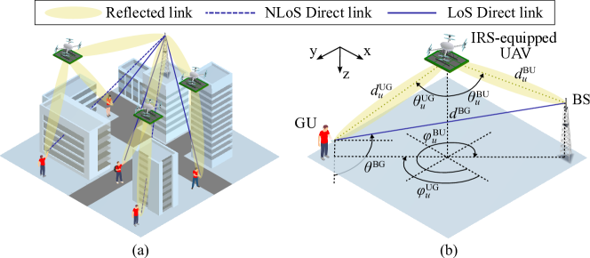
Figure 1: Overview of (a) the reference scenario and (b) the channel model geometry.

II System Model

The investigated scenario, illustrated in Figure 1, considers a mission that lasts $K$ seconds, in which $U$ IRS-equipped UAVs, flying at speed $v_{u}\in\mathbb{R}$, $u=1,\ldots,U$, improve the channel quality between a set of $G$ GUs and the BS, through a proper signal reflection. In this Section, for the sake of notations, the discussion considers the communication of a GU, in a given subcarrier centered in $f\ $\mathrm{H}\mathrm{z}$$, at a certain time instant. The positions of the drones, the GU, and the BS are denoted as $\textbf{q}_{u}^{\text{\tiny{U}}}=[x^{\text{\tiny{U}}}_{u},y^{\text{\tiny{U}}}_{u},z_{u}^{\text{\tiny{U}}}]^{\mathsf{T}}\in\mathbb{R}^{3}$, $\textbf{q}^{\text{\tiny{G}}}=[x^{\text{\tiny{G}}},y^{\text{\tiny{G}}},z^{\text{\tiny{G}}}]^{\mathsf{T}}\in\mathbb{R}^{3}$, and $\textbf{q}^{\text{\tiny{B}}}=[x^{\text{\tiny{B}}},y^{\text{\tiny{B}}},z^{\text{\tiny{B}}}]^{\mathsf{T}}\in\mathbb{R}^{3}$. Accordingly, the far-field distances $d^{\text{\tiny{UG}}}_{u}$, $d^{\text{\tiny{BU}}}_{u}$, and $d^{\text{\tiny{BG}}}$ are defined as $d^{\text{\tiny{ab}}}=\left\lVert\textbf{q}^{\text{\tiny{a}}}-\textbf{q}^{\text{\tiny{b}}}\right\rVert$, with a, b $\in\{U,G,B\}$.

IRSs are composed by $N=N^{\text{\tiny{R}}}\times N^{\text{\tiny{C}}}$ PRUs, having the size $w=d^{\text{\tiny{X}}}\times d^{\text{\tiny{Y}}}\ $\mathrm{m}^{2}$$, with $d^{\text{\tiny{X}}}=d^{\text{\tiny{Y}}}\triangleq d$ being the length of the element sides. The midpoint of each PRU, with respect to the center of the IRS, is $d\left[(i-\frac{1}{2}),(i^{\prime}-\frac{1}{2})\right]^{\mathsf{T}}$ with $i=1-\frac{N^{\text{\tiny{C}}}}{2},\ldots,\frac{N^{\text{\tiny{C}}}}{2},i^{\prime}=1-\frac{N^{\text{\tiny{R}}}}{2},\ldots,\frac{N^{\text{\tiny{R}}}}{2}$. The PRUs are grouped into $P$ patches of $M=M^{\text{\tiny{R}}}\times M^{\text{\tiny{C}}}$ elements, each one indexed as $m=1,\ldots,M$. Moreover, each patch reflects the incident signal according to a phase shift matrix $\mathbf{\Phi}_{u,p}\in\mathbb{C}^{M\times M}$, with $p=1,\ldots,P$, defined as

$$\mathbf{\Phi}_{u,p}=\text{diag}\bigg{(} e^{j\phi_{u,p,1}},\ldots,e^{j\phi_{u,p,m}},\ldots,e^{j\phi_{u,p,M}}\bigg{)},$$ (1)

where $\phi_{u,p,m}\in[-\pi,\pi)$. It is worth specifying that for ease of readability, all the IRSs have the same number and size of patches but the model is straightforward extensible. This is demonstrated by the actual implementation of the simulator, described in the Section IV-B.

Finally, define $\{\theta^{\text{\tiny{UG}}}_{u},\theta^{\text{\tiny{BU}}}_{u}\}$ and $\{\varphi^{\text{\tiny{UG}}}_{u},\varphi^{\text{\tiny{BU}}}_{u}\}$ as the inclination and azimuth angles between the center of the IRS and the GU/BS as $\theta^{\text{\tiny{ab}}}=\mathrm{acos}\left(\frac{z^{\text{\tiny{a}}}-z^{\text{\tiny{b}}}}{d^{\text{\tiny{ab}}}}\right)$ and $\varphi^{\text{\tiny{ab}}}=\mathrm{atan2}\left(\frac{y^{\text{\tiny{a}}}-y^{\text{\tiny{b}}}}{x^{\text{\tiny{a}}}-x^{\text{\tiny{b}}}}\right)$. Similarly, $\theta^{\text{\tiny{BG}}}$ denotes the inclination angle related to the direct GU-BS link with respect to the GU.

III Channel Model

The communication system employs the OFDMA scheme, which prevents interference among the involved entities. The GU and the BS employ a single-antenna for data exchange, that, together with each IRS element, are characterized by power radiation pattern functions (including antenna gains) denoted by $F^{\text{\tiny{GU}}}$, $F^{\text{\tiny{BS}}}$, and $F^{\text{\tiny{IRS}}}$.

According to [20], the channel gain $g^{\text{\tiny{BG}}}\in\mathbb{C}$ of the direct GU-BS link is

$$g^{\text{\tiny{BG}}}=\sqrt{\beta^{\text{\tiny{BG}}}{d^{\text{\tiny{BG}}}}^{-\alpha}F^{\text{\tiny{BG}}}}h^{\text{\tiny{BG}}},$$ (2)

where $\beta^{\text{\tiny{BG}}}$ is the channel power gain at the reference distance of 1 m, $\alpha$ is the pathloss exponent, and $F^{\text{\tiny{BG}}}=F^{\text{\tiny{BS}}}F^{\text{\tiny{GU}}}$. Moreover, $h^{\text{\tiny{BG}}}$ is the channel coefficient, which accounts for the small-scale fading and follows a circularly-symmetric non-central complex gaussian distribution. The envelope $|h^{\text{\tiny{BG}}}|$ is generally Rician [21], with K-factor $\kappa^{\text{\tiny{BG}}}$ and average power $\Omega^{\text{\tiny{BG}}}=1$. Specifically, $\kappa^{\text{\tiny{BG}}}$ can be expressed as a function of the elevation angle and reads

$$\kappa^{\text{\tiny{BG}}}=\kappa^{\text{\tiny{MIN}}}\exp\left(\frac{2}{\pi}\ln{\frac{\kappa^{\text{\tiny{MAX}}}}{\kappa^{\text{\tiny{MIN}}}}}\left|\frac{\pi}{2}-\theta^{\text{\tiny{BG}}}\right|\right),$$ (3)

with $\kappa^{\text{\tiny{MIN}}}$ and $\kappa^{\text{\tiny{MAX}}}$ the minimum and maximum possible K-factors, respectively. With similar definitions, given the $p$-th patch of the $u$-th UAV, the channel gains $\textbf{g}_{u,p}^{\text{\tiny{UG}}}\in\mathbb{C}^{M}$ and $\textbf{g}_{u,p}^{\text{\tiny{BU}}}\in\mathbb{C}^{M}$, related to the GU and the BS, can be formulated as follows:

$$\textbf{g}_{u,p}^{\text{\tiny{UG}}}=\sqrt{\beta^{\text{\tiny{UG}}}{d^{\text{\tiny{UG}}}_{u}}^{-2}F^{\text{\tiny{UG}}}}\textbf{h}_{u,p}^{\text{\tiny{UG}}},$$ (4)

$$\textbf{g}_{u,p}^{\text{\tiny{BU}}}=\sqrt{\beta^{\text{\tiny{BU}}}{d^{\text{\tiny{BU}}}_{u}}^{-2}F^{\text{\tiny{BU}}}}\textbf{h}_{u,p}^{\text{\tiny{BU}}},$$ (5)

whose envelopes are characterized by K-factors $\kappa_{u}^{\text{\tiny{UG}}}$ and $\kappa_{u}^{\text{\tiny{BU}}}$. Since each patch $p$ coherently reflects the incident signal from the BS towards a GU and vice versa, all the phase shifts can be described in terms of two parameters, $\phi_{u,p}^{\text{\tiny{X}}}$ and $\phi_{u,p}^{\text{\tiny{Y}}}$, thus reducing the degrees of freedom by imposing that:

$$\ell\left(\left(i-\frac{1}{2}\right)\phi_{u,p}^{\text{\tiny{X}}}+\left(i^{\prime}-\frac{1}{2}\right)\phi_{u,p}^{\text{\tiny{Y}}}\right)=\phi_{u,p,m},$$ (6)

being $\ell=\frac{2\pi fd}{c}$ and $c$ the speed of light. The overall channel gain that characterizes the communication of a GU served by the swarm is

$$\Gamma=\sum_{u=1}^{U}\sum_{p=1}^{P}{\textbf{g}^{\text{\tiny{BU}}}_{u,p}}^{\mathsf{T}}\mathbf{\Phi}_{u,p}\textbf{g}_{u,p}^{\text{\tiny{UG}}}+g^{\text{\tiny{BG}}},$$ (7)

which is intractable due to the product of complex gaussians. Nonetheless, according to [20], the envelope can be approximated to a Rician random variable having K-factor $\kappa=\frac{\nu^{2}}{2{\sigma}^{2}}$ and average power $\Omega=\nu^{2}+2{\sigma}^{2}$, with $\nu^{2}$ and $2{\sigma}^{2}$ defined as

$$\nu^{2} =\sum^{U}_{u=1}\sum^{P}_{p=1}\mu_{u,p}^{2}+2\sum_{u\geq u^{\prime}}\sum_{p>p^{\prime}}|\mu_{u,p}||\mu_{u^{\prime},p^{\prime}}|\cos\left(\omega_{u}-\omega_{u^{\prime}}\right)$$

$$+\!\lambda^{2}\overline{\kappa}^{\text{\tiny{BG}}}\!+\!2\sum^{U}_{u=1}\sum^{P}_{p=1}|\mu_{u,p}||\lambda\sqrt{\overline{\kappa}^{\text{\tiny{BG}}}}|\cos\left(\omega_{u}\!+\!\frac{\ell d_{g}^{\text{\tiny{BG}}}}{d}\right),$$ (8)

$$2\sigma^{2} =N\sum_{u=1}^{U}\eta^{2}_{u}\widetilde{\kappa}^{\text{\tiny{BUG}}}_{u}+\lambda^{2}\widetilde{\kappa}^{\text{\tiny{BG}}},$$ (9)

with

$$\mu_{u,p}=\eta_{u}\sqrt{\overline{\kappa}_{u}^{\text{\tiny{BUG}}}}\frac{\sin\left(\frac{\ell M^{\text{\tiny{C}}}}{2}\psi^{\text{\tiny{X}}}_{u,p}\right)\sin\left(\frac{\ell M^{\text{\tiny{R}}}}{2}\psi^{\text{\tiny{Y}}}_{u,p}\right)}{\sin\left(\frac{\ell}{2}\psi^{\text{\tiny{X}}}_{u,p}\right)\sin\left(\frac{\ell}{2}\psi^{\text{\tiny{Y}}}_{u,p}\right)}e^{-j\omega_{u}},$$ (10)

$$\overline{\kappa}_{u}^{\text{\tiny{BUG}}}=\frac{\kappa_{u}^{\text{\tiny{BU}}}\kappa_{u}^{\text{\tiny{UG}}}}{(\kappa_{u}^{\text{\tiny{BU}}}+1)(\kappa_{u}^{\text{\tiny{UG}}}+1)},\widetilde{\kappa}_{u}^{\text{\tiny{BUG}}}=\frac{\kappa_{u}^{\text{\tiny{BU}}}+\kappa_{u}^{\text{\tiny{UG}}}}{(\kappa_{u}^{\text{\tiny{BU}}}+1)(\kappa_{u}^{\text{\tiny{UG}}}+1)},$$ (11)

$$\psi^{\text{\tiny{X}}}_{u,p}=\sin{\theta^{\text{\tiny{BU}}}_{u}}\cos{\varphi^{\text{\tiny{BU}}}_{u}}+\sin{\theta^{\text{\tiny{UG}}}_{u}}\cos{\varphi^{\text{\tiny{UG}}}_{u}}+\phi_{u,p}^{\text{\tiny{X}}},$$ (12)

$$\psi^{\text{\tiny{Y}}}_{u,p}=\sin{\theta^{\text{\tiny{BU}}}_{u}}\sin{\varphi^{\text{\tiny{BU}}}_{u}}+\sin{\theta^{\text{\tiny{UG}}}_{u}}\sin{\varphi^{\text{\tiny{UG}}}_{u}}+\phi_{u,p}^{\text{\tiny{Y}}},$$ (13)

$\omega_{u}=\ell\left(d^{\text{\tiny{BU}}}_{u}+d^{\text{\tiny{UG}}}_{u}\right),\qquad\eta_{u}=\sqrt{\beta^{\text{\tiny{BUG}}}{d^{\text{\tiny{BU}}}_{u}}^{-2}{d^{\text{\tiny{UG}}}_{u}}^{-2}F^{\text{\tiny{BUG}}}}$, $\lambda~{}=~{}\sqrt{\beta^{\text{\tiny{BG}}}{d^{\text{\tiny{BG}}}}^{-\alpha}F^{\text{\tiny{BG}}})}$, $F^{\text{\tiny{BUG}}}=F^{\text{\tiny{BU}}}F^{\text{\tiny{UG}}}$, $\overline{\kappa}^{\text{\tiny{BG}}}=\frac{\kappa^{\text{\tiny{BG}}}}{\kappa^{\text{\tiny{BG}}}+1}$, $\widetilde{\kappa}^{\text{\tiny{BG}}}=\left(\kappa^{\text{\tiny{BG}}}+1\right)^{-1}$, and $\beta^{\text{\tiny{BUG}}}=\beta^{\text{\tiny{BU}}}\beta^{\text{\tiny{UG}}}$.

Finally, given an outage probability $\varepsilon$, the channel power gain can be lowerbounded [20] as

$$\Gamma_{\varepsilon} =\frac{\zeta^{2}\Omega}{2(\kappa+1)},$$ (14)

$$\zeta =\begin{cases}\sqrt{-2\log(1-\varepsilon)}e^{\frac{\kappa}{2}},&\!\!\!\!\!\text{for }\kappa\leq\frac{K_{0}^{2}}{2}\\ \sqrt{2\kappa}+\frac{1}{2Q^{-1}(\varepsilon)}\times\\ \quad\log\left(\frac{\sqrt{2\kappa}}{\sqrt{2\kappa}-Q^{-1}(\varepsilon)}\right)-Q^{-1}(\varepsilon),&\!\!\!\!\!\text{for }\kappa>\frac{K_{0}^{2}}{2}\end{cases}$$ (15)

with $Q^{-1}(x)$ being the inverse Q-function and $K_{0}$ the intersection of the sub-functions at $\sqrt{2\kappa}>Q^{-1}(\varepsilon)$. Equations (14) and (15) will be used in the proposed IoD-Sim IRS module.

IV Software Design

The proposed module is designed according to the structure of IoD-Sim. To this end, a general overview of the simulator architecture is given, thus providing a comprehensive description of the abstraction layers and the available software facilities. Then, the IRS module is introduced, along with the software definition and the mathematical model implementation. Finally, the configuration of a simple scenario, via JSON parameters, is discussed.

IV-A IoD Sim

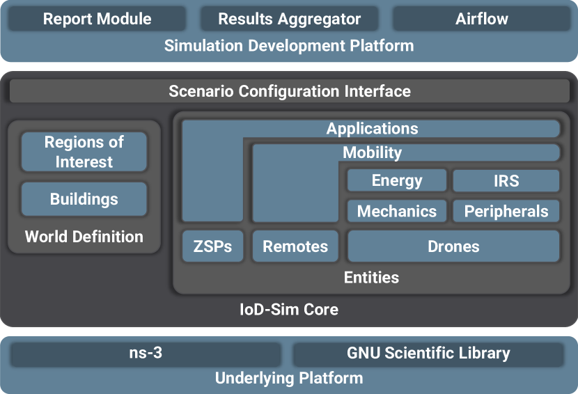
Figure 2: IoD-Sim architecture integrated with the IRS module.

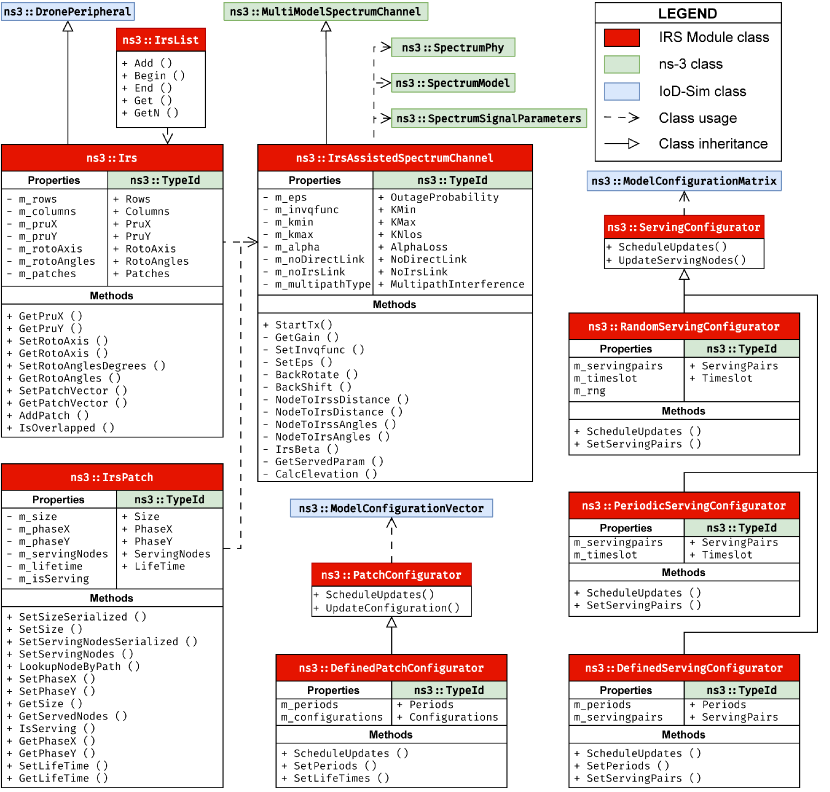
Figure 3: Class diagram of the IRS extension implemented in IoD-Sim.

IoD-Sim [19] is a comprehensive simulation platform designed to assess UAV-enabled communication systems with ease. The architecture, illustrated in Figure 2, is a software stack composed by three logical layers, namely Underlying Platform, IoD-Sim Core, and Simulation Development Platform. The former provides a solid foundation of established software used for (i) network simulation, i.e., ns-3 [22], and (ii) optimized mathematical computation, i.e., GNU Scientific Library (GSL).

On top of that, the simulator presents IoD-Sim Core which mainly (i) introduces IoD entities, (ii) defines the reference 3D world, and (iii) simulates remote cloud services. In particular, drones are mechanically modeled by taking into account physical and power-consumption properties, such as mass, rotor disk area, drag coefficient of the rotor blades, and battery model. Moreover, UAV motion can be simulated through one of the manifold mobility models, which easily allow trajectory design starting from a set of points of interest. Further, applications and peripherals enable the simulation of multiple use cases, spanning from telemetry reporting to multi-stack relaying, video recording, and streaming. To provide services that go beyond classical network coverage, Zone Service Providers are also implemented in the simulator, which are specialized BSs that leverages the cyber-physical environment to provide local Air Traffic Control (ATC), weather forecast, and cloud services to a geographical zone of interest. On these premises, the platform enables the design of a fully integrated terrestrial/non-terrestrial drone network.

All the features that characterize the IoD-Sim Core are made available through a low-code and user-friendly Simulation Development Platform, which is conceived to easily create and maintain a scenario configuration through either a block-based GUI, named Airflow, or a JSON file. These designs are then parsed and executed, without requiring deep understanding of the underlying C++ code.

Finally, the software generates simulation reports in the form of plain text and structured data sets that can be processed through conventional data-analysis tools. These may be used to evaluate and graphically analyze UAVs trajectories, network traffic, and application-specific KPIs.

IV-B IRS Simulation Module

The proposed module is implemented on top of IoD-Sim, which represents a solid foundation to design and assess the desired IRS-assisted UAV-aided scenarios. Accordingly, multiple classes, depicted in Figure 3, are hereby introduced to enhance the IoD-Sim Core.

In particular, PHY layer communications are implemented by means of the ns3::IrsAssistedSpectrumChannel class, which extends the channel simulation capabilities originally provided by ns3::MultiModelSpectrumChannel. Specifically, this object evaluates the overall receiver gain, derived in Section III, which considers both the reflected links, introduced by the IRSs, and the original direct link between the nodes of interest.

Figure 4: JSON configuration properties of an IRS with a patch highlighted in yellow.

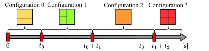
Figure 5: Different patch configurations applied over time, following the ns3::DefinedPatchConfigurator logic.

The IRS is described by the ns3::Irs class, which extends the generic peripheral one, i.e., ns3::DronePeripheral [19, Sec. V.B]. The adoption of this interface benefits the implementation of the IRS as a device. In fact, it is possible to have (i) a state that can be put in either OFF, IDLE, or ON, and (ii) an associated energy consumption model (even though it is negligible with respect to the main components that drain the UAV battery). All ns3::Irs instances are referenced by a global register named ns3::IrsList, allowing them to be easily reachable through object paths formatted as /IrsList/[IRS_Global_Index].

As illustrated in Figure 4, the IRS is characterized by different properties that can be set through the ns3::TypeId attributes: Rows and Columns for the IRS size; PruX and PruY for the dimension of each PRU; RotoAxis and RotoAngles to indicate an ordered sequence of axes and their rotation in degrees, respectively. For instance, RotoAxis = ["X_AXIS"] and RotoAngles = [180] indicate that the IRS should be rotated by 180 degrees around the x axis, i.e., the surface faces the ground.

Each ns3::Irs is organized into one or more ns3::IrsPatch, whose dimensions can be specified through the Size property. This property has four values corresponding to the starting and ending PRUs’ indexes along the x and y axes, i.e, Size[0:1] and Size[2:3]. Once the patches dimensions are set, they can be configured to support the communication of a specific pair of Serving Nodes.

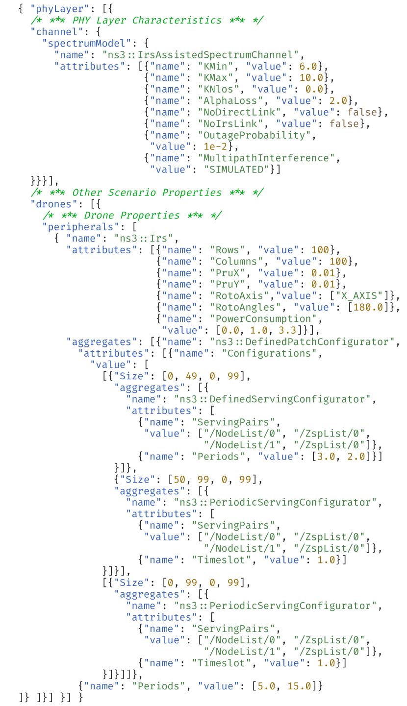
Figure 6: Extract of a JSON scenario configuration that employs the IRS-aware spectrum channel model and installs a single IRS on a drone to serve a pair of nodes.

In order to provide a flexible and dynamic configurations at runtime, the proposed implementation offers additional configurator classes ns3::PatchConfigurator and ns3::ServingConfigurator. The former sets up the number and size of IRSs patches, called Patch Configurators. The latter schedules the nodes to be served by each patch, namely Serving Configurators.

For what concerns Patch Configurators, the ns3::DefinedPatchConfigurator represents a basic reference already available in the module.

Parameter	Value	Parameter	Value
Simulated Area	$400\times$400\text{\,}\mathrm{[}\mathrm{m}^{2}\mathrm{]}$$	KMax	$10\text{\,}\mathrm{[}\mathrm{d}\mathrm{B}\mathrm{]}$
KMin	$6\text{\,}\mathrm{[}\mathrm{d}\mathrm{B}\mathrm{]}$	KNlos	$0\text{\,}\mathrm{[}\mathrm{d}\mathrm{B}\mathrm{]}$
AlphaLoss	$\{3,\,4\}\ $\mathrm{[}\#\mathrm{]}$$	NoIrsLink	false
OutageProbability	$0.01\text{\,}\mathrm{[}\#\mathrm{]}$	NoDirectLink	false
RotoAxis	["X_AXIS"]	RotoAngles	$[180.0]\ $\mathrm{[}\mathrm{d}\mathrm{e}\mathrm{g}\mathrm{]}$$
PruX, PruY	$0.01\text{\,}\mathrm{m}$	UE, eNB Power	$24,\,$49\text{\,}\mathrm{[}\mathrm{d}\mathrm{B}\mathrm{m}\mathrm{]}$$

TABLE II: Parameter settings.

It allows the definition of different patch setups that the IRS adopts over time, as depicted in Figure 5. It can be observed that the simulation starts by dividing the IRS in two parts, as specified by Configuration 0. At time $t_{0}$, the patches are reorganized to follow the map given by Configuration 1. This logic reiterates twice more, until the end of the simulation.

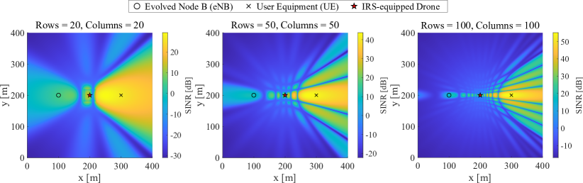
Figure 7: Comparison among downlink REMs for different IRS sizes.

Regarding the nodes to be served, instead, they can be scheduled according to one of the available Serving Configurator algorithms: ns3::DefinedServingConfigurator which enables the definition of a list of node pairs to assist for different time intervals; ns3::PeriodicServingConfigurator which schedules node pairs in round-robin fashion for the same amount of time; ns3::RandomServingConfigurator randomly chooses which node pair to assist for a fixed time interval.

The Simulation Development Platform allows an easy configuration of (i) the channel model properties, (ii) the IRSs setup, and (iii) the scheduling plans through a JSON file, as shown in Figure 6. Such feature is enabled by the ns3::ModelConfigurationVector and ns3::ModelConfigurationMatrix, which have been developed as an extension in the Scenario Configuration Interface, in order to dynamically apply different configurations at runtime. As it can be noticed, the channel model can be configured through the parameters that are described in Section III, where OutageProbability is $\epsilon$, KMin is $\kappa^{\text{\tiny MIN}}$, KMax is $\kappa^{\text{\tiny MAX}}$, and AlphaLoss is $\alpha$. Furthermore, NoDirectLink and NoIrsLink represent booleans useful to analyze use cases where the direct and the reflected links are suppressed. MultipathInterference, instead, can assume three different values which affect the interference introduced by the direct and reflected links (the second cosine in Equation (8)): DESTRUCTIVE for a purely destructive interference (i.e., worst case), SIMULATED for the actual one, and CONSTRUCTIVE for no interference at all (i.e., best case). Finally, KNlos is the K-factor adopted when the direct link is in Non Line of Sight (NLoS). Such parameters can be further tuned to simulate better or worse channel conditions according to the simulation design requirements.

IRS configuration can be declared in the JSON as a drone peripheral. In the example given in Figure 6, two configurations are applied to the IRS, with different time durations, specified in Periods. In the first one, the IRS is split in half with two patches: one patch assists the links of two GU, with global index 0 and 1, for three and two seconds, respectively; the second one periodically serves the same users for one second each. Further, in the second configuration, the whole IRS is used for 15 seconds to serve both nodes in round-robin fashion for one second each. Finally, a power consumption, related to the IRS controller, is also defined.

V Simulation Campaign

The entire simulation campaign revolves around the features studied for both the mathematical model, described in Section III, and the IoD-Sim implementation, presented in Section IV-B. Three different scenarios are designed and assessed hereby to validate the features introduced by the IRS module, adopting the parameters reported in Table II, if not otherwise specified. Furthermore, all the scenarios are tested using one communication technology only, i.e., Long Term Evolution (LTE), with a fixed bandwidth of $5\text{\,}\mathrm{M}\mathrm{H}\mathrm{z}$ and 25 resource blocks. In particular, all these scenarios consider a Evolved Node-B (eNB), acting as a ZSP/BS, and a set of User Equipments, acting as nodes/GUs, that experience different SINR levels due to pathloss and LoS conditions. To this end, IRS-equipped UAVs are employed to assist the communication links. The overall performance achieved through the aid of the IRS are compared, analyzed, and discussed via several KPIs, such as REM, SINR, maximum achievable rate, and average throughput.

V-A Scenario #1

The first Scenario considers an area with a building of $20\times 20\times$25\text{\,}\mathrm{m}^{3}$$, placed at $[200,200,0]$, that obstructs the direct link between an eNB and a UE, located at $[100,200,30]$ and $[300,200,0]$, respectively. To support the communication between these two nodes, an IRS-equipped UAV hovers $50\text{\,}\mathrm{m}$ over the building, thus re-establishing the LoS. The overall Scenario is depicted in Figure 7, which also illustrates the downlink REM at the ground level with a resolution of $16\text{\,}\mathrm{s}\mathrm{a}\mathrm{m}\mathrm{p}\mathrm{l}\mathrm{e}\mathrm{s}\mathrm{/}\mathrm{m}^{2}$. It is worth specifying that, for the sake of the analysis, the contribution of the eNB-UE direct link is temporarily neglected. The radiation fingerprints exhibit two main properties: as the number of PRUs increases (i) the main lobe pointing at the target node becomes narrower and (ii) the perceived SINR increases as well. However, these benefits come at the price of a larger IRS, which implies higher costs and footprint.

Figure 8 depicts the same scenario from a different point of view. The direct link is not neglected anymore and it is considered an IRS of fixed size $100\times 100$ elements, with a varying attenuation factor $\alpha=\{3,\,4\}$ adopted for the direct link. Clearly, this case highlights the shadowing effect due to the presence of the building, which is more evident with $\alpha=3$, since the direct link is less attenuated. At the same time, with $\alpha=4$, it is more noticeable a weaker shadow surrounding the building, which is its projection on the ground as a result of the IRS reflections, i.e., UAV-UE NLoS link. Moreover, it can be noticed a slight ripple effect due to fast-fading phenomena as a consequence of multipath interference.

Lastly, Figure 9 shows the channel conditions between the eNB and UE in terms of SINR and maximum achievable data rate in uplink. This time, multiple configurations investigate the presence and also the absence of the building, labeled with “LoS” and “NLoS”. Moreover, the total absence of the eNB-UE direct link is considered, marked as “No direct link”. In terms of SINR, illustrated on the left, the first obvious observation is that, for a given $\alpha$, the LoS cases are always better than the NLoS ones. Moreover, for a low number of elements, the curves with $\alpha=3$ start with a better SINR with respect to the ones characterized by $\alpha=4$. However, as the IRS becomes larger, the less attenuated case in NLoS conditions, i.e., $\alpha=3$, is characterized by a significant destructive interference phenomena, as it can be noticed by comparing it with the ”No direct link“ curve. These unwanted effects can be prevented with a proper design of the scenario geometry, i.e., the communication actors should be correctly aligned. Lastly, for a very large number of elements, all cases converge to ”No direct link“, since the reflected link overshadows the direct one. For what concerns the maximum achievable rate, depicted on the right, it follows a trend that is similar to the SINR. It can be observed that, as the number of PRUs grows, the curves overlap due to Modulation and Coding Scheme (MCS) switching [23], until the rate saturates at $18.336\text{\,}\mathrm{M}\mathrm{b}\mathrm{p}\mathrm{s}$.

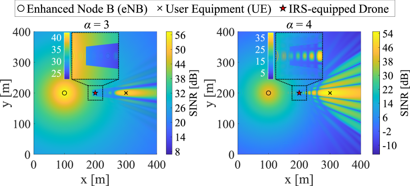
Figure 8: Downlink REMs for different attenuation factors.

Figure 9: Uplink maximum achievable rate and SINR under different channel conditions.

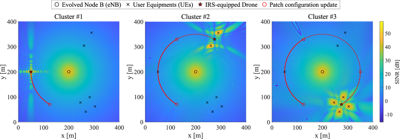
Figure 10: REMs taken exactly when the drone results orthogonal to each cluster.

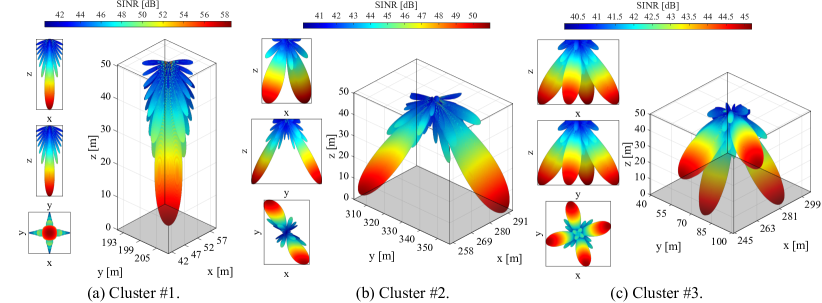
Figure 11: The 3D radiation patterns of the IRS serving different clusters.

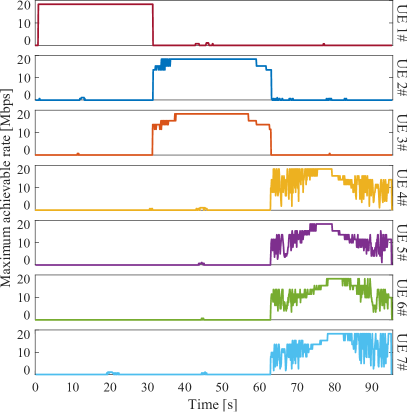
Figure 12: Uplink maximum achievable rate.

V-B Scenario #2

This scenario considers the presence of three clusters: (i) Cluster #1 is made by 1 UE placed in $[50,200,0]$, (ii) Cluster #2 has 2 UEs positioned at $\{[260,303.923,0],[290,355.885,0]\}$, and (iii) Cluster #3 is characterized by 4 UEs located at $\{[282.765,99.074,0]$, $[303.978,62.331,0]$, $[267.235,41.118,0]$, $[246.022,77.86,0]\}$. All the UEs exchange data with an eNB with the support of an IRS-equipped UAV. The direct UE-eNB link is characterized by the pathloss exponent $\alpha=4$. The goal is to fairly serve each cluster through a IRS of $100\times 100$ elements. To this end, the drone follows a circular trajectory of radius $150\text{\,}\mathrm{m}$, at a constant speed of $10\text{\,}\mathrm{m}\mathrm{/}\mathrm{s}$, that intersects the center of each cluster. The circumference is equally divided into three arcs, for which a suitable IRS configuration is set to serve the UEs of interest for $\sim$31.416\text{\,}\mathrm{s}$$.

The described scenario is depicted in Figure 10, which also shows the downlink REM at three different instants corresponding to the UAV being orthogonal to the center of each cluster. As it can be seen, the reflected signal power yields a different radiation pattern on the ground, depending on the adopted IRS configuration. As already seen in Scenario #1, this case is subject to the interference between direct and reflected links, i.e., multipath. Additionally, this effect is exacerbated by the presence of patches configured to serve different members of the same cluster, i.e., the IRS self-interference. Furthermore, the SINR is inversely proportional to the number of users to be served. This behavior is more evident in Figure 11, where the signal beams produced by the IRS are depicted, with a peak SINR of $\sim$58.61\text{\,}\mathrm{d}\mathrm{B}$$ for Cluster #1, $\sim$50.98\text{\,}\mathrm{d}\mathrm{B}$$ for Cluster #2, and $\sim$45.19\text{\,}\mathrm{d}\mathrm{B}$$ for Cluster #3. Specifically, the SINR lowers since the surface is equally divided among the nodes of the target cluster. It is worth noting that, differently from the Clusters #1 and #3, the two beams depicted in Figure 11b are not symmetrical, as can be seen in the x-z and y-z projections, due to the rectangular shape of the patches.

For the sake of completeness, in Figure 12 it is investigated the uplink maximum achievable rate for all the UEs, since it is more critical with respect to the downlink one. The contribution of the UAV is crucial to allow the communication between these nodes and the eNB. Indeed, when the UEs are no longer supported by the drone, the data rate drops to zero due to the high loss characterizing the direct link. Otherwise, it can be observed time-discrete variations of the rate, which are caused by the MCS switching. This is due to (i) the variation of the UAV-GUs distance and (ii) the fast-fading effect, which clearly worsens as the number of served UEs increases. Moreover, when the UAV is closest to a UE, the theoretical maximum rate of $18.336\text{\,}\mathrm{M}\mathrm{b}\mathrm{p}\mathrm{s}$ is reached, as already seen in Figure 9 of Scenario #1.

V-C Scenario #3

The last scenario investigates all the available Serving Configurators described in Section IV-B, in the context of a smart city. Indeed, the urban environment is particularly useful to analyze both LoS and NLoS cases. As depicted in the left of Figure 13, multiple buildings and an uniform grid of 25 UEs are considered. Each UE communicates with an eNB placed on the top of the bottom-left building, at $30\text{\,}\mathrm{m}$ of height. As it can be noted, in the right of Figure 13, the downlink REM shows the shadowing effect due to the presence of buildings, which obstruct the LoS between some UEs and the eNB. As a consequence, there are nodes that cannot communicate, since the SINR is under the threshold, according to the ns3::MiErrorModel [24]. To cope with this issue, the communication system is enhanced with one and then four IRS-equipped UAVs. In the former case, the UAV is placed in $[200,200,50]$, whereas in the latter the UAVs are located at $\{[100,200,50]$, $[200,300,50]$, $[300,200,50]$, $[200,100,50]\}$.

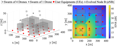
Figure 13: Simulated smart city scenario.

Figure 14: UEs average throughput adopting different Serving Configurators.

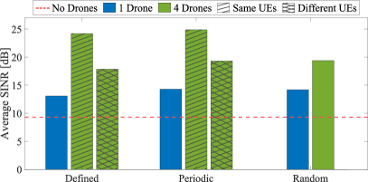
Figure 15: UEs average SINR adopting different Serving Configurators.

In order to saturate the LTE capacity, a live streaming traffic is simulated for a mission that lasts $75\text{\,}\mathrm{s}$. With this aim, the ns3::UdpEchoClientApplication is employed, which leverages the User Datagram Protocol (UDP) protocol to transmit a packet of $64\text{\,}\mathrm{K}\mathrm{i}\mathrm{B}$, i.e., the maximum possible size, every $0.03\text{\,}\mathrm{s}$. All the three proposed Serving Configurators described in Section IV-B are tested, labeled as Defined, Periodic, and Random. Specifically, the former is set up to exclusively serve the nodes that have an SINR below the threshold. The last two, instead, serve all the nodes. Moreover, a baseline is also considered (the red dashed line) in which no drones assist the UEs, which have to rely solely on the direct link with the eNB. The results, in terms of average throughput and SINR, are reported in Figures 14 and 15, respectively. In both Figures, the blue bars indicate the case where only one IRS-equipped drone is employed, whereas the green ones consider a swarm of 4 UAVs. In the latter case, patterns are used to distinguish two different approaches: “Same UEs” refers to the case in which all drones simultaneously assist a given UE in each time interval; vice versa, “Different UEs” indicates that all drones serve distinct UEs. For obvious reasons, the “Random” case do not discuss such a difference.

It is evident that, with respect to the baseline approach, the employment of IRSs leads to an improvement in both the average throughput and SINR, of at least $\sim 27.66\%$ and $\sim 40.6\%$, respectively. Of course, these benefits become more prominent as the number of drones increases. Among the adopted configurators, it can be noted that there are no major differences in terms of SINR. Indeed, even if in different orders, UEs are served for about the same time and with the same bandwidth. Nonetheless, the Periodic presents slightly better performances. However, when the average throughput is considered, the Periodic configurator (which performs very similar to the random one) does not guarantee the same benefits brought by the Defined one. Indeed, the latter focuses on serving those nodes which demand more signal power to reach the required minimum SINR, which in turn produces an higher overall system throughput. A similar rationale can be applied when, given a configurator, “Same UEs” and “Different UEs” are compared. In fact, serving distinct UEs at the same time allows them to use a higher MCS, which yields a greater average throughput, even if the corresponding SINR are comparable.

VI Conclusions

The IoD represents a major leap in telecommunications, as it enables on-demand network coverage and a high degree of versatility. At the same time, IRSs allow to control the environmental conditions of the radio channel, thus leading to noticeable improvements in communication quality. As drones and IRSs clearly represent key-enablers for 6G communications, this work proposes a module based on the IoD-Sim platform, which enables the development of future communication systems where this two technologies can be integrated. This module represents a flexible solution thanks to the available general schedulers for IRS patches.

Despite the manifold features already available, the IRS module will be improved in the future, with more efforts focused on:

1. Accurate power consumption model of IRSs.

2. Performance assessment of this module with mmWave simulations, to assess the performance of systems that go beyond classical sub-6GHz communications.

3. Comparison of these new emerging systems with AF solutions, employed in 5G network backhaul.

4. Real-time attitude controls for the IRS in order to follow a target mobile node.

5. Enhanced configurators with feedback loop that choose to serve nodes depending on their channel conditions.

6. Channel model aware of the specific material obstructing the LoS, in order to choose the most suitable K-factor and pathloss coefficient.

Hopefully, this work will stimulate the scientific community to improve the intelligence of these emerging devices in multiple directions. The emergence of a flourishing and empowering community on open-source collaboration platforms will ultimately determine the success of future development endeavors.

Giovanni Grieco received the Dr. Eng. degree (with honors) in Telecommunications Engineering from Politecnico di Bari, Bari, Italy in October 2021. His research interests include Internet of Drones, Cybersecurity, and Future Networking Architectures. He is the principal maintainer of IoD_Sim. Since 2021, he has been a Ph.D. student at the Department of Electrical and Information Engineering at Politecnico di Bari.

Giovanni Iacovelli received the Ph.D. in electrical and information engineering from Politecnico di Bari, Bari, Italy, in December 2022. His research interests include Internet of Drones, Machine Learning, Optimization and Telecommunications. Currently, he is a Research Fellow at the Department of Electrical and Information Engineering, Politecnico di Bari.

Daniele Pugliese received his Bachelor’s degree (with honors) in Computer and Automation Engineering in December 2021 from Politecnico di Bari, Bari, Italy, where he is currently a Master’s Student in Telecommunications Engineering. Since March 2022 he is a research fellow at the Department of Electrical and Information Engineering, Politecnico di Bari.

Domenico Striccoli received, with honors, the Dr. Eng. Degree in Electronic Engineering in April 2000, and the Ph.D. degree in April 2004, both from the Politecnico di Bari, Italy. In 2005 he joined the DIASS Department of Politecnico di Bari in Taranto as Assistant Professor in Telecommunications. Actually he teaches fundamental courses in the field of Telecommunications at Department of Electrical and Information Engineering (DEI) of Politecnico di Bari, where he holds the position of Assistant Professor in Telecommunications. Dr. Striccoli has authored numerous scientific papers on various topics related to electronic engineering. His work has been published in esteemed international journals and presented at leading scientific conferences.

L. Alfredo Grieco is a full professor in telecommunications at Politecnico di Bari. His research interests include Internet of Things, Future Internet Architectures, and Nano-communications. He serves as Founder Editor in Chief of the Internet Technology Letters journal (Wiley) and as Associate Editor of the IEEE Transactions on Vehicular Technology journal (for which he has been awarded as top editor in 2012, 2017, and 2020).

References

- [1] M. Giordani, M. Polese, M. Mezzavilla, S. Rangan, and M. Zorzi, “Toward 6g networks: Use cases and technologies,” IEEE Communications Magazine, vol. 58, no. 3, pp. 55–61, 2020.
- [2] M. A. Javed, T. N. Nguyen, J. Mirza, J. Ahmed, and B. Ali, “Reliable communications for cybertwin-driven 6g iovs using intelligent reflecting surfaces,” IEEE Transactions on Industrial Informatics, vol. 18, no. 11, pp. 7454–7462, 2022.
- [3] B. Ji, Y. Wang, L. Xing, C. Li, Y. Wang, H. Wen, and K. Huang, “Irs-driven cybersecurity of healthcare cyber physical systems,” IEEE Transactions on Network Science and Engineering, pp. 1–10, 2022.
- [4] P. Boccadoro, D. Striccoli, and L. A. Grieco, “An Extensive Survey on the Internet of Drones,” Ad Hoc Netw., vol. 122, p. 102600, 2021.
- [5] M. M. Azari, S. Solanki, S. Chatzinotas, O. Kodheli, H. Sallouha, A. Colpaert, J. F. Mendoza Montoya, S. Pollin, A. Haqiqatnejad, A. Mostaani, E. Lagunas, and B. Ottersten, “Evolution of non-terrestrial networks from 5g to 6g: A survey,” IEEE Communications Surveys & Tutorials, vol. 24, no. 4, pp. 2633–2672, 2022.
- [6] R. Bajracharya, R. Shrestha, S. Kim, and H. Jung, “6g nr-u based wireless infrastructure uav: Standardization, opportunities, challenges and future scopes,” IEEE Access, vol. 10, pp. 30 536–30 555, 2022.
- [7] G. Geraci, A. Garcia-Rodriguez, M. M. Azari, A. Lozano, M. Mezzavilla, S. Chatzinotas, Y. Chen, S. Rangan, and M. D. Renzo, “What will the future of uav cellular communications be? a flight from 5g to 6g,” IEEE Communications Surveys & Tutorials, vol. 24, no. 3, pp. 1304–1335, 2022.
- [8] “Ieee standard for local and metropolitan area networks–part 15.7: Short-range wireless optical communication using visible light,” IEEE Std 802.15.7-2011, pp. 1–309, 2011.
- [9] “Ieee draft standard for wireless multi-media networks,” IEEE P802.15.3-Rev.B/D4.0, January 2023, pp. 1–685, 2023.
- [10] S. Gong, X. Lu, D. T. Hoang, D. Niyato, L. Shu, D. I. Kim, and Y.-C. Liang, “Toward smart wireless communications via intelligent reflecting surfaces: A contemporary survey,” IEEE Communications Surveys & Tutorials, vol. 22, no. 4, pp. 2283–2314, 2020.
- [11] G. Iacovelli, A. Coluccia, and L. A. Grieco, “Channel Gain Lower Bound for IRS-Assisted UAV-Aided Communications,” IEEE Commun. Lett., vol. 25, no. 12, pp. 3805–3809, 2021.
- [12] L. Hao, A. Fastenbauer, S. Schwarz, and M. Rupp, “Towards System Level Simulation of Reconfigurable Intelligent Surfaces,” in 2022 International Symposium ELMAR, 2022, pp. 81–84.
- [13] H. Choi and J. Choi, “WiThRay: Versatile 3D Simulator for Intelligent Reflecting Surface-aided MmWave Systems,” in 2021 International Symposium on Antennas and Propagation (ISAP), 2021, pp. 1–2.
- [14] E. Basar and I. Yildirim, “SimRIS Channel Simulator for Reconfigurable Intelligent Surface-Empowered Communication Systems,” in 2020 IEEE Latin-American Conference on Communications (LATINCOM), 2020, pp. 1–6.
- [15] M. Pagin, M. Giordani, A. A. Gargari, A. Rech, F. Moretto, S. Tomasin, J. Gambini, and M. Zorzi, “End-to-End Simulation of 5G Networks Assisted by IRS and AF Relays,” in 2022 20th Mediterranean Communication and Computer Networking Conference (MedComNet), 2022, pp. 150–157.
- [16] B. Sihlbom, M. I. Poulakis, and M. D. Renzo, “Reconfigurable Intelligent Surfaces: Performance Assessment Through a System-Level Simulator,” IEEE Wireless Communications, pp. 1–10, 2022.
- [17] Q. GU, D. WU, X. SU, H. Wang, J. Cui, and Y. Yuan, “System-level Simulation of RIS assisted Wireless Communications System,” in GLOBECOM 2022 - 2022 IEEE Global Communications Conference, 2022, pp. 1540–1545.
- [18] 3GPP, “5G; Study on channel model for frequencies from 0.5 to 100 GHz,” 3rd Generation Partnership Project (3GPP), Technical Report (TR) 38.901, 11 2020, version 16.1.0. [Online]. Available: https://portal.3gpp.org/desktopmodules/Specifications/SpecificationDetails.aspx?specificationId=3173
- [19] G. Grieco, G. Iacovelli, P. Boccadoro, and L. Grieco, “Internet of drones simulator: Design, implementation, and performance evaluation,” 03 2022.
- [20] G. Iacovelli, A. Coluccia, and L. A. Grieco, “Multi-UAV IRS-assisted Communications: Multi-Node Channel Modeling and Fair Sum-Rate Optimization via Deep Reinforcement Learning,” 2 2023. [Online]. Available: https://www.techrxiv.org/articles/preprint/Multi-UAV_IRS-assisted_Communications_Multi-Node_Channel_Modeling_and_Fair_Sum-Rate_Optimization_via_Deep_Reinforcement_Learning/22102652
- [21] M. A. Al-Jarrah, K.-H. Park, A. Al-Dweik, and M.-S. Alouini, “Error Rate Analysis of Amplitude-Coherent Detection over Rician Fading Channels with Receiver Diversity,” IEEE Trans. Wireless Commun., vol. 19, no. 1, pp. 134–147, 2019.
- [22] G. F. Riley and T. R. Henderson, The ns-3 Network Simulator. Berlin, Heidelberg: Springer Berlin Heidelberg, 2010, pp. 15–34. [Online]. Available: https://doi.org/10.1007/978-3-642-12331-3_2
- [23] 3GPP, “LTE; Evolved Universal Terrestrial Radio Access (E-UTRA); Physical layer procedures,” 3rd Generation Partnership Project (3GPP), Technical Specification (TS) 36.213, 11 2008, version 8.3.0 Release 8. [Online]. Available: https://portal.3gpp.org/desktopmodules/Specifications/SpecificationDetails.aspx?specificationId=2427
- [24] M. Mezzavilla, M. Miozzo, M. Rossi, N. Baldo, and M. Zorzi, “A lightweight and accurate link abstraction model for the simulation of lte networks in ns-3,” in Proceedings of the 15th ACM international conference on Modeling, analysis and simulation of wireless and mobile systems, 2012, pp. 55–60.