Diffusion Bridge Mixture Transports, Schrödinger Bridge Problems and Generative Modeling

Abstract

The dynamic Schrödinger bridge problem seeks a stochastic process that defines a transport between two target probability measures, while optimally satisfying the criteria of being closest, in terms of Kullback-Leibler divergence, to a reference process. We propose a novel sampling-based iterative algorithm, the iterated diffusion bridge mixture (IDBM) procedure, aimed at solving the dynamic Schrödinger bridge problem. The IDBM procedure exhibits the attractive property of realizing a valid transport between the target probability measures at each iteration. We perform an initial theoretical investigation of the IDBM procedure, establishing its convergence properties. The theoretical findings are complemented by numerical experiments illustrating the competitive performance of the IDBM procedure. Recent advancements in generative modeling employ the time-reversal of a diffusion process to define a generative process that approximately transports a simple distribution to the data distribution. As an alternative, we propose utilizing the first iteration of the IDBM procedure as an approximation-free method for realizing this transport. This approach offers greater flexibility in selecting the generative process dynamics and exhibits accelerated training and superior sample quality over larger discretization intervals. In terms of implementation, the necessary modifications are minimally intrusive, being limited to the training loss definition.

Keywords: measure transport; coupling; Schrödinger bridge; iterative proportional fitting; diffusion process; stochastic differential equation; score-matching; generative modeling.

1 Introduction

Generating samples from a given distribution is a central topic in computational statistics and machine learning. In recent years, transportation of probability measures has gained considerable attention as a computational tool for sampling. The underlying concept entails generating samples from a complex distribution by first obtaining samples from a simpler distribution and subsequently computing a suitably constructed map of these samples (El Moselhy and Marzouk, 2012; Marzouk et al., 2016). Let us consider the following definition: given two probability measures $Γ$ and $ϒ$, a transport from $Γ$ to $ϒ$ is defined as a map $h(X,ε)$, where $ε$ is an independent auxiliary random element, such that if $X∼Γ$ (i.e., $X$ is distributed according to $Γ$), then $Y=h(X,ε)$ satisfies $Y∼ϒ$. This broad definition encompasses both deterministic and random transports and includes a wide range of sampling methods, such as Markov Chain Monte Carlo (Brooks et al., 2011), normalizing flows (Papamakarios et al., 2021), and score-based generative modeling (Ho et al., 2020; Song et al., 2021).

To narrow down the extensive class of possible transports, we can identify the optimal transport according to a suitably chosen criterion. This paper addresses a more generalized version of the optimization problem initially posed by Schrödinger in 1931 (Léonard, 2014b). In this context, both $Γ$ and $ϒ$ are defined on the same $d$-dimensional Euclidean space. The optimization space comprises $d$-dimensional diffusion processes on the time interval $[0,τ]$, constrained to have initial distribution $Γ$ and terminal distribution $ϒ$. Optimality is achieved by minimizing the Kullback-Leibler divergence to a reference diffusion process. The optimal map $Y=h(X,ε)$ is thus obtained by defining $ε$ as the $d$-dimensional Brownian motion on $[0,τ]$ which drives the optimal diffusion process started at $X$, with terminal value $Y$. This seemingly intricate procedure of defining a transport is of practical relevance. When the reference diffusion is given by a scaled Brownian motion $σW_{t}$, for some $σ>0$, $(X,h(X,ε))$ solves the Euclidean entropy-regularized optimal transport (EOT) problem (Peyré and Cuturi, 2020, Chapter 4) for the regularization level $2σ^{2}$. EOT provides a more tractable alternative to solving the optimal transport (OT) problem. However, in high-dimensional settings, solving the EOT problem remains challenging. The dynamic formulation, achieved by inflating the original space where $Γ$ and $ϒ$ are supported so that they correspond to the initial-terminal distributions of a stochastic process, is essential to recent computational advancements in these demanding settings. Specifically, Bortoli et al. (2021); Vargas et al. (2021) rely on a time-reversal result for diffusion processes to implement sampling-based iterative algorithms aimed at solving the dynamic Schrödinger bridge problem.

1.1 Our Contributions

In this work, we begin by reviewing the theory of Schrödinger bridge problems in their various forms, as well as the approaches developed by Bortoli et al. (2021); Vargas et al. (2021). We establish that sampling-based time-reversal approaches suffer from a simulation-inference mismatch. Specifically, at each iteration, samples from the previous iteration are utilized to infer a new diffusion process, but relevant regions of the state space can be left unexplored. This issue is particularly prominent in scenarios characterized by a low level of randomness in the reference process. This is problematic when the goal is to solve the OT problem: for the EOT solution to closely approximate the OT solution, the scale $σ$ of the reference diffusion $σW_{t}$ must be small.

The primary contribution of this work is the development of a novel sampling-based iterative algorithm, the IDBM procedure, for addressing the dynamic Schrödinger bridge problem. We begin by noting that the problem’s solution, i.e. the optimal diffusion process, can be represented as a mixture of diffusion bridges, with the mixing occurring over the bridges’ endpoints. In general, processes constructed in this manner are not diffusion processes (Jamison, 1974, 1975). The IDBM procedure involves the following iterative steps: (i) constructing a stochastic process as a mixture of diffusion bridges such that its initial-terminal distribution forms a coupling of the target probability measures $Γ$ and $ϒ$; (ii) matching the marginal distributions of the stochastic process generated in (i) with a diffusion process; (iii) updating the coupling from step (i) with the initial-terminal distributions of the diffusion obtained in step (ii). The diffusion process of step (ii) is inferred based on samples from the stochastic process of step (i). Crucially, as both processes share the same marginal distributions, no simulation-inference mismatch occurs. In this study, we conduct an initial theoretical examination of the IDBM procedure, establishing its convergence properties toward the solution to the dynamic Schrödinger bridge problem. Additionally, we carry out empirical evaluations of the IDBM procedure in comparison to the IPF procedure, highlighting its robustness.

The recent advancements in score-based generative approaches (Song et al., 2021; Rombach et al., 2022) have demonstrated remarkable generative quality in visual applications by leveraging the time-reversal of a reference diffusion process to define the sampling process. To elaborate further, the reference diffusion’s dynamics are selected based on a decoupling criterion, which requires the process’s terminal value to be approximately independent of the process’s initial value. The reference process’s initial distribution is assumed to be the empirical distribution of a dataset of interest, or a slightly perturbed version of it. The time reversal of the reference diffusion, complemented by a dataset-independent initial distribution, defines the sampling process. In this work, we propose to utilize the first iteration of the IDBM procedure as an alternative method of defining a sampling process targeting a dataset of interest. Under this proposal, the reference diffusion’s dynamics are no longer constrained by decoupling considerations. We conduct an empirical evaluation of the resulting transport, demonstrating its competitiveness for visual applications in comparison to the approach of Song et al. (2021). Remarkably, the proposed approach exhibits accelerated training and superior sample quality at larger discretization intervals without fine-tuning the involved hyperparameters. From a practitioner standpoint, implementing the proposed method requires minimal changes, which are confined to the training loss definition.

1.2 Structure of the Paper

The paper is structured as follows. In Section 2 we introduce the Schrödinger bridge problem in its various forms, the IPF procedure, its time-reversal sampling-based implementations for the case of a reference diffusion process, and score-based generative modeling. The IDBM procedure, its convergence properties, and suitable training objectives are presented in Section 3. In Section 4 we define the class of reference stochastic differential equations (SDE) considered in the applications, which are carried out in Section 6. Section 5 discusses relevant connections and Section 7 provides concluding remarks for the paper. Proofs, auxiliary formulae and visualizations, code listings and a table summarizing the notation used throughout this work are deferred to the Appendices.

1.3 Notation and Preliminaries

In light of the methodological focus of the present work, we refrain from discussing some of the more technical aspects. The excellent treatises by Léonard (2014b, a) provide a formal account of the preliminaries discussed below and of the developments of Section 2.1. To aid the reader, a summary of the main notation is provided in Table 3 (Appendix E).

All the stochastic processes we are concerned with are defined over the continuous time interval $[0,τ]$, have state space $ℝ^{d}$, and are continuous, for some constants $τ>0$ and $d≥1$. A realization of a stochastic process, or path, is an element $x∈𝒞([0,τ],ℝ^{d})$, the space of continuous functions from $[0,τ]$ to $ℝ^{d}$.

We denote each probability measure (PM, or distribution, law) with an uppercase letter. For a PM $P$, $X∼P$ denotes that $X$ is a random element with distribution $P$. Let $n≥1$ and $t_{1},…,t_{n}∈[0,τ]$. We denote the collection of PMs over $𝒞([0,τ],ℝ^{d})$ with $𝒫_{𝒞}$ and the collection of PMs over $ℝ^{d×n}$ with $𝒫_{n}$. When $P∈𝒫_{n}$ admits a density with respect to the Lebesgue measure on $ℝ^{d×n}$ we denote this density with the same lowercase letter (here $p$). For $P∈𝒫_{𝒞}$, we denote with $P_{t_{1},…,t_{n}}∈𝒫_{n}$ the marginalization of $P$ at $t_{1},…,t_{n}$ and with $P_{\textbullet|t_{1},…,t_{n}}∈𝒫_{𝒞}$ the conditioning of $P$ given the values at times $t_{1},…,t_{n}$. More explicitly, if $X∼P∈𝒫_{𝒞}$, we have $P_{t_{1},…,t_{n}}(A_{1},…,A_{n})=\Pr[X_{t_{1}}∈A_{1},…,X_{t_{n}}∈A_{n}]$ and $P_{\textbullet|t_{1},…,t_{n}}(A|x_{1},…,x_{n})=\Pr[X∈A|X_{t_{1}}=x_{1},…,X_{t_{n}}=x_{n}]$. A path PM can be defined via a mixture: if $Ψ∈𝒫_{n}$ and $P∈𝒫_{𝒞}$, let $Q=ΨP_{\textbullet|t_{1},…,t_{n}}$ stand for $Q(A)=∫P_{\textbullet|t_{1},…,t_{n}}(A|x_{1},…,x_{n})Ψ(dx_{1},…,dx_{n})$. That is, $Q$ is obtained by pinning down $X∼P$ at times $t_{1},…,t_{n}$, and taking a mixture with respect to $Ψ$ over the pinned down values. With this notation, the marginal-conditional decomposition of $P∈𝒫_{𝒞}$ is $P=P_{t_{1},…,t_{n}}P_{\textbullet|t_{1},…,t_{n}}$. If $P,Q∈𝒫_{𝒞}$, and $P$ is absolutely continuous with respect to $Q$ ($P≪Q$) with density $(dP/dQ)(x)$, the marginal-conditional decomposition of $(dP/dQ)(x)$ is $(dP/dQ)(x)=(dP_{t_{1},…,t_{n}}/dQ_{t_{1},…,t_{n}})(x_{t_{1}},…,x_{t_{n}})×(dP_{\textbullet|t_{1},…,t_{n}}/dQ_{\textbullet|t_{1},…,t_{n}})(x)$.

Given two PMs $Γ,ϒ∈𝒫_{1}$, we define $𝒫_{𝒞}(Γ,ϒ)⊆𝒫_{𝒞}$ as the collection of PMs having $Γ$ as initial distribution and $ϒ$ as terminal distribution. Hence, $P∈𝒫_{𝒞}(Γ,ϒ)$ transports $Γ$ to $ϒ$ ($P_{0}=Γ,P_{τ}=ϒ$), while its time reversal transports $ϒ$ to $Γ$. We write $𝒫_{𝒞}(Γ,□)$ when only the initial distribution is fixed, and $𝒫_{𝒞}(□,ϒ)$ when only the terminal distribution is fixed. We define $𝒫_{2}(Γ,ϒ)⊆𝒫_{2}$ as the collection of PMs with prescribed marginal distributions $Γ$ and $ϒ$, i.e. the collection of couplings between $Γ$ and $ϒ$. We write $𝒫_{2}(Γ,□)$ ($𝒫_{2}(□,ϒ)$) when only the first (second) marginal distribution is fixed. For $P∈𝒫_{2}$, we write $P_{0},P_{τ}$ to denote respectively the first and second marginal, and denote the conditional distributions with $P_{\textbullet|0}$ and $P_{\textbullet|τ}$. With this notation, for $P∈𝒫_{𝒞}∪𝒫_{2}$ we have $P=P_{0}P_{\textbullet|0}=P_{τ}P_{\textbullet|τ}$.

We write $𝒰(0,τ)$ for the uniform distribution on $(0,τ)$, $𝒩_{d}(μ,Σ)$ for the $d$-variate normal distribution with mean $μ∈ℝ^{d}$ and covariance $Σ∈ℝ^{d×d}$. We write $X_{i}\overset{\text{\tiny{iid}}}{∼}P$ to denote that each random elements $X_{i}$ is independent and identically distributed according to a PM $P$. For $S,R$ two PMs on the same space, the Kullback-Leibler (KL) divergence from $S$ to $R$ is defined as $D_{KL}(S\mathbin{\textbardbl}R)≔𝔼_{S}[\log(\frac{dS}{dR})]$ whenever $S≪R$, $+∞$ otherwise.

We denote identity matrices with $I$, and transposition of a square matrix $A$ with $Aᵀ$. We use the notation $[A]_{i}$ and $[A]_{i,j}$ to denote indexing respectively of a vector and of a matrix. The Euclidean norm of a vector $V$ is denoted by $\textbardbl V\textbardbl$.

If $X∼P∈𝒫_{𝒞}$, we denote the time reversal of $X$ with $\overline{X}$, that is $\overline{X}_{t}≔X_{τ-t}$ ($t∈[0,τ]$). The time reversal of $P$ itself is defined as $\overline{P}[A]≔P[\overline{A}]$, $\overline{A}≔\{x:x_{τ-t}∈A\}$, so that $\overline{X}∼\overline{P}$. Note that $E_{P}[f(X)]=E_{\overline{P}}[f(\overline{X})]$ for any integrable $f:𝒞([0,τ],ℝ^{d})\textrightarrow ℝ$. Thorough the paper we set $𝔯≔τ-t$.

Without further mention, all SDE drift coefficients are assumed to be $ℝ^{d}$-valued and all SDE diffusion coefficients are assumed to be $ℝ^{d×d}$-valued. Most SDEs, and associated diffusion solutions, are denoted with the same letter $X$. To avoid ambiguity, we clearly denote the corresponding probability laws. Similarly, we denote most $ℝ^{d}$-valued standard Brownian motions with $W$. It is understood that all Brownian motions driving different SDEs are independent nonetheless.

2 Schrödinger Bridge Problems

In Section 2.1 we review the theory of Schrödinger bridge problems in both dynamic and static formulations. We initially consider the generic setting of continuous stochastic processes before specializing to the case of a diffusion reference measures. In Sections 2.2 and 2.3, we discuss the classical iterative algorithm employed in the numerical solution to Schrödinger bridge problems, focusing on recent contributions that rely on a time reversal argument for diffusion processes. Throughout our discussion, we adopt a path space, or continuous-time, perspective. This perspective not only provides clarity but also highlights the connection with a sequential estimation problem for diffusion processes. For the sake of completeness, we review the basics of simulation and inference for SDEs in Section 2.4. Finally, in Section 2.5, review score-based generative modeling, emphasizing its connections to the dynamic Schrödinger bridge problem.

2.1 Dynamic, Static and Half Versions

For $Γ,ϒ∈𝒫_{1}$ and $R∈𝒫_{𝒞}$, the solution to the dynamic Schrödinger bridge problem $(\mathrm{S_{dyn}})$ is given by

$$S^{*}(Γ,ϒ,R,𝒫_{𝒞})≔\operatorname*{arg\,min}_{S∈𝒫_{𝒞}(Γ,ϒ)}D_{KL}(S\mathbin{\textbardbl}R).$$

$(\mathrm{S_{dyn}})$ seeks a stochastic process transporting an initial distribution $Γ$ to a terminal distribution $ϒ$, while achieving minimum Kullback-Leibler (KL) divergence to the reference law $R$. For a given $S∈𝒫_{𝒞}$, $S≪R$, the marginal-conditional decompositions for PMs and densities give

$$D_{KL}(S\mathbin{\textbardbl}R) =𝔼_{S_{0,τ}}\Big{[}𝔼_{S_{\textbullet|0,τ}}\Big{[}\log\Big{(}\frac{dS_{0,τ}}{dR_{0,τ}}(x_{0},x_{τ})\frac{dS_{\textbullet|0,τ}}{dR_{\textbullet|0,τ}}(x)\Big{)}\Big{]}\Big{]}$$

$$=D_{KL}(S_{0,τ}\mathbin{\textbardbl}R_{0,τ})+𝔼_{S_{0,τ}}[D_{KL}(S_{\textbullet|0,τ}\mathbin{\textbardbl}R_{\textbullet|0,τ})].$$ (1)

The second term of 1 is minimized by $S^{*}_{\textbullet|0,τ}(Γ,ϒ,R,𝒫_{𝒞})=R_{\textbullet|0,τ}$, independently of $Γ,ϒ$, yielding the representation of $S^{*}(Γ,ϒ,R,𝒫_{𝒞})$ as a mixture of the reference process pinned down at its initial and terminal values. The mixing distribution $S^{*}_{0,τ}(Γ,ϒ,R,𝒫_{𝒞})$ over the initial and terminal values minimizes the first term of 1, i.e. it solves a specific instance of the following problem.

For $Γ,ϒ∈𝒫_{1}$ and $B∈𝒫_{2}$, the solution to the static Schrödinger bridge problem $(\mathrm{S_{sta}})$ is given by

$$S^{*}(Γ,ϒ,B,𝒫_{2})≔\operatorname*{arg\,min}_{C∈𝒫_{2}(Γ,ϒ)}D_{KL}(C\mathbin{\textbardbl}B).$$

$(\mathrm{S_{sta}})$ differs from $(\mathrm{S_{dyn}})$ in the optimization space: $𝒫_{2}$ instead of $𝒫_{𝒞}$. With this notation, $S^{*}_{0,τ}(Γ,ϒ,R,𝒫_{𝒞})=S^{*}(Γ,ϒ,R_{0,τ},𝒫_{2})$, the solution to $(\mathrm{S_{sta}})$ for $B=R_{0,τ}$. The solution to $(\mathrm{S_{dyn}})$ is then $S^{*}(Γ,ϒ,R,𝒫_{𝒞})=S^{*}(Γ,ϒ,R_{0,τ},𝒫_{2})R_{\textbullet|0,τ}$. Vice versa, if $S^{*}(Γ,ϒ,R,𝒫_{𝒞})$ solves $(\mathrm{S_{dyn}})$, then $S_{0,τ}^{*}(Γ,ϒ,R,𝒫_{𝒞})$ solves $(\mathrm{S_{sta}})$ for $B=R_{0,τ}$. From this point onward, $(\mathrm{S_{sta}})$ is always understood to be associated to the corresponding $(\mathrm{S_{dyn}})$, i.e. we will only consider $(\mathrm{S_{sta}})$ for $B=R_{0,τ}$. It established in Rüschendorf and Thomsen (1993) that, if there is a $C∈𝒫_{2}(Γ,ϒ)$ such that $D_{KL}(C\mathbin{\textbardbl}R_{0,τ})<∞$, then $(\mathrm{S_{sta}})$ admits a solution, which is unique. This hypothesis is assumed to hold thorough the paper.

We introduce an additional axis among which to classify Schrödinger bridge problems, covering both dynamic $(\mathrm{H_{dyn}})$ and static $(\mathrm{H_{sta}})$ variants jointly for conciseness. Thus, let $𝒫$ be either $𝒫_{𝒞}$ (case of $(\mathrm{H_{dyn}})$) or $𝒫_{2}$ (case of $(\mathrm{H_{sta}})$). For $Γ,ϒ∈𝒫_{1}$, $Q∈𝒫$, the solutions to the forward and to the backward Schrödinger half bridge problems are respectively given by

$$S^{*}(Γ,□,Q,𝒫) ≔\operatorname*{arg\,min}_{H∈𝒫(Γ,□)}D_{KL}(H\mathbin{\textbardbl}Q),$$

$$S^{*}(□,ϒ,Q,𝒫) ≔\operatorname*{arg\,min}_{H∈𝒫(□,ϒ)}D_{KL}(H\mathbin{\textbardbl}Q).$$

In contrast to $(\mathrm{S_{dyn}})$ and $(\mathrm{S_{sta}})$, only one of the marginal conditions is enforced. The forward and backward half bridge problems admit simpler solutions which form the basis of the developments of Section 2.2. Proceeding as in 1, it can be established that for $H∈𝒫$ such that $H≪Q$

$$D_{KL}(H\mathbin{\textbardbl}Q) =D_{KL}(H_{0}\mathbin{\textbardbl}Q_{0})+𝔼_{H_{0}}[D_{KL}(H_{\textbullet|0}\mathbin{\textbardbl}Q_{\textbullet|0})]$$ (2)

$$=D_{KL}(H_{τ}\mathbin{\textbardbl}Q_{τ})+𝔼_{H_{τ}}[D_{KL}(H_{\textbullet|τ}\mathbin{\textbardbl}Q_{\textbullet|τ})],$$

from which we obtain the half bridge solutions $S^{*}(Γ,□,Q,𝒫)=ΓQ_{\textbullet|0}$ and $S^{*}(□,ϒ,Q,𝒫)=ϒQ_{\textbullet|τ}$. That is, one of the endpoint (or marginal, for $(\mathrm{H_{sta}})$) distributions of $Q=Q_{0}Q_{\textbullet|0}=Q_{τ}Q_{\textbullet|τ}$ is replaced by one of $Γ,ϒ$ while keeping the associated conditional distribution of $Q$ constant. In the case of $(\mathrm{H_{dyn}})$, it thus suffices to propagate the initial (terminal) distribution $Γ$ ($ϒ$) through the forward (backward) dynamics of $Q$: $Q_{\textbullet|0}$ ($Q_{\textbullet|τ}$).

$R_{0}$ plays a minor role in $(\mathrm{S_{dyn}})$. From 2 applied with $Q=R$, $H∈𝒫_{𝒞}$, either $R_{0}$ is such that $(\mathrm{S_{dyn}})$ do not admit any solution (when $D_{KL}(S\mathbin{\textbardbl}R)=+∞$ for every $S∈𝒫_{𝒞}(Γ,ϒ)$), or the solution to $(\mathrm{S_{dyn}})$ exists, is unique, and is independent of $R_{0}$. This work is concerned with the case where $R$ is given by the solution to a $d$-dimensional SDE, i.e. a diffusion process (Øksendal, 2003; Friedman, 1975). We consider the following reference SDE, with initial distribution $Γ$ (without loss of generality),

$$dX_{t}=μ_{R}(X_{t},t)dt+σ_{R}(X_{t},t)dW_{t},\quad t∈[0,τ],$$ (3)

$$X_{0}∼Γ.$$

Thorough the paper, it is assumed that 3 admits a unique (weak, non-explosive) solution, whose law defines the reference law $R=ΓR_{\textbullet|0}$. It is also assumed that $R≪R^{\circ}$ where $R^{\circ}$ is the law of the unique solution to 3 with $μ_{R}(x,t)=0$, and that $Σ_{R}(x,t)≔σ_{R}(x,t)σ_{R}(x,t)ᵀ$ is invertible. These are mild assumptions. The law $R_{\textbullet|0}$ only depends on the drift coefficient $f(x,t)$ and on the diffusion coefficient $σ_{R}(x,t)$.

In concluding this section, it is noteworthy that solving $(\mathrm{S_{sta}})$ is equivalent to solving a corresponding EOT problem. We seek a solution $S^{*}(Γ,ϒ,R_{0,τ},𝒫_{2})$, and for the sake of simplicity we examine the case where $Γ,ϒ,R_{0,τ}$ and $C∈𝒫_{2}(Γ,ϒ)$ all admits densities with respect to Lebesgue measures. Therefore,

$$S^{*}(Γ,ϒ,R_{0,τ},𝒫_{2})=\operatorname*{arg\,min}_{C∈𝒫_{2}(Γ,ϒ)}𝔼_{C}[-\log r_{τ|0}(X_{τ}|X_{0})]+H(C).$$

Here $H(C)≔𝔼_{C}[\log c(X_{0},X_{τ})]$ is the entropy of $C$. Given the same assumption, we consider a cost function $κ(x,y):ℝ^{d}×ℝ^{d}\textrightarrow ℝ$ and two target marginal distributions $Γ,ϒ$ of interest. The solution to the EOT problem with regularization $ε>0$ is then defined as

$$EOT^{*}(Γ,ϒ,κ,ε)≔\operatorname*{arg\,min}_{C∈𝒫_{2}(Γ,ϒ)}𝔼_{C}[κ(X_{0},X_{τ})]+εH(C).$$ (4)

By judiciously selecting the reference measure $R$, it becomes feasible to solve a corresponding EOT problem of interest. For example, if $R$ is associated to $dX_{t}=σdW_{t}$ for a scalar $σ>0$, then $S^{*}(Γ,ϒ,R_{0,τ},𝒫_{2})=EOT^{*}(Γ,ϒ,\textbardbl x-y\textbardbl^{2},2σ^{2})$. Consequently, $S^{*}(Γ,ϒ,R_{0,τ},𝒫_{2})$ is the solution to the Euclidean EOT problem for regularization $ε=2σ^{2}$. The arguments presented here carry over to the more generic measure-theoretic setting (Peyré and Cuturi, 2020, Remark 4.2).

2.2 Iterative Proportional Fitting (IPF)

The main tool employed in the numerical solution to $(\mathrm{S_{dyn}})$ and $(\mathrm{S_{sta}})$ is an iterative procedure, known in the literature under a variety of names. In $(\mathrm{S_{sta}})$, when $Γ$ and $ϒ$ admit Lebesgue densities $γ(□)$ and $υ(□)$, the term Fortet iterations (Fortet, 1940) is used. Instead, when $Γ$ and $ϒ$ concentrate all mass on a finite set of values, the term iterative proportional fitting procedure (Deming and Stephan, 1940) is used. In the same setting, due to the equivalence between $(\mathrm{S_{sta}})$ and EOT, the same procedure is also known as Sinkhorn algorithm. Finally, the term IPF can be used in the context of the measure-theoretic formulation of Ruschendorf (1995), including the dynamic version $(\mathrm{S_{dyn}})$ (Bernton et al., 2019). In this work, we utilize the IPF term.

Algorithm 1 IPF

1:$Γ,ϒ,R_{\textbullet|0},n$

2:$\{F^{(i)}\}_{i=1}^{n}$

3:$F^{(0)}\textleftarrow ΓR_{\textbullet|0}$

4:for $i=1,…,n$ do

5:   if $i$ is even then

6:     $F^{(i)}\textleftarrow ΓF^{(i-1)}_{\textbullet|0}$ $\triangleright$ forward IPF

7:   else

8:    $F^{(i)}\textleftarrow ϒF^{(i-1)}_{\textbullet|τ}$ $\triangleright$ backward IPF

9:   end if

10:end for

For $(\mathrm{S_{sta}})$ or $(\mathrm{S_{dyn}})$, the IPF procedure (Algorithm 1) is obtained by iteratively solving the forward and backward half bridge problems starting from the reference measure $R$. More precisely, let $𝒫$ be either $𝒫_{𝒞}$ or $𝒫_{2}$, $R∈𝒫$, $Γ,ϒ∈𝒫_{1}$, and assume that $R=ΓR_{\textbullet|0}$. The IPF procedure is defined by the iterates $F^{(0)}=R=S^{*}(Γ,□,R,𝒫)$, $F^{(1)}=S^{*}(□,ϒ,F^{(0)},𝒫)$, $F^{(2)}=S^{*}(Γ,□,F^{(1)},𝒫)$, and so on. Under appropriate conditions (Ruschendorf, 1995), the PMs $F^{(i)}$ associated with the IPF iterates of Algorithm 1 converge in total variation (TV) metric and in KL divergence to $S^{*}(Γ,ϒ,R,𝒫)$ as $i\textrightarrow∞$. Note that our choice of indexing of the IPF iterations differs from the prior literature, where indexing starts from $1$. In this work, indexing reflects the number of learning problems that needs to be solved in order to produce samples from the corresponding IPF iteration. As simulation from 3 is in general feasible (Section 2.4), and can be carried out exactly for the specifications of interest (Section 4), no learning is required to produce samples from $F^{(0)}$.

For $(\mathrm{S_{dyn}})$, and specifically for the case of a reference diffusion law $R$, Bortoli et al. (2021); Vargas et al. (2021) introduce implementations of Algorithm 1 that rely on a time reversal result for diffusion processes (Anderson, 1982). Let $X$ be the $d$-dimensional diffusion process with law $P∈𝒫_{𝒞}$ arising as unique solution to the SDE

$$dX_{t}=μ(X_{t},t)dt+σ_{R}(X_{t},t)dW_{t},\quad t∈[0,τ],$$ (5)

$$X_{0}∼P_{0}.$$

Under suitable conditions, the time reversed process $\overline{X}_{t}≔X_{τ-t}$ is still a diffusion process, associated to the SDE

$$d\overline{X}_{t}=υ(\overline{X}_{t},t)dt+σ_{R}(\overline{X}_{t},𝔯)dW_{t},\quad t∈[0,τ],$$ (6)

$$υ(x,t)≔-μ(x,𝔯)+∇⋅Σ_{R}(x,𝔯)+Σ_{R}(x,𝔯)∇_{x}\log p_{𝔯}(x),$$

$$\overline{X}_{0}∼P_{τ}.$$

In 6 $𝔯≔τ-t$, $p_{t}(x)$ is the Lebesgue density of the marginal distribution $P_{t}$, and the $d$-dimensional vector $∇⋅Σ_{R}(x,t)$ is defined as $[∇⋅Σ_{R}(x,t)]_{i}\ ≔∑_{j=1}^{d}∇_{x_{j}}[Σ_{R}(x,t)]_{i,j}$, $1≤i≤d$. We refer to Haussmann and Pardoux (1986); Millet et al. (1989) for the conditions required on 5 for the time reversal 6 to hold.

2.3 Diffusion IPF as Iterative Simulation-Inference

Bortoli et al. (2021); Vargas et al. (2021) propose sampling-based implementations of Algorithm 1. At iteration $i≥1$, samples are generated from $F^{(i-1)}$ to construct an approximation to $F^{(i)}$. This approximation is used in turn to generate samples from $F^{(i)}$, which form the input to iteration $i+1$.

Let $F^{(i-1)}$ be a diffusion associated to a SDE (which holds for $i=1$, as $F^{(0)}=R$). We show that $F^{(i)}$ is also a diffusion associated to a different SDE. First, lines 4 and 6 of Algorithm 1 are modified respectively to $F^{(i)}\textleftarrow Γ\overline{F}^{(i-1)}_{\textbullet|0}$ and $F^{(i)}\textleftarrow ϒ\overline{F}^{(i-1)}_{\textbullet|0}$. With this choice, the path PMs associated to backward IPF iterations are defined over a reverse (relatively to the forward IPF iterations) timescale. Denote the drift and diffusion coefficients associated to $F^{(i-1)}$ respectively with $μ_{F}^{(i-1)}(x,t)$ and $σ_{R}(x,t)$, so that $μ_{F}^{(0)}(x,t)=μ_{R}(x,t)$. It will become clear shortly why the diffusion coefficient is independent of $i$. If $i$ is even, we have $F^{(i)}_{0}=Γ$, otherwise $F^{(i)}_{0}=ϒ$. Thus, for all $i≥1$, $F^{(i)}=F^{(i)}_{0}\overline{F}^{(i-1)}_{\textbullet|0}$. Crucially, from the time reversal result of Anderson (1982), we know that $\overline{F}^{(i-1)}$ is the law of the diffusion associated to

$$d\overline{X}_{t}^{(i-1)}=μ_{F}^{(i)}(\overline{X}^{(i-1)}_{t},t)dt+σ_{R}(\overline{X}^{(i-1)}_{t},𝔯)dW_{t},\quad t∈[0,τ],$$ (7)

$$μ_{F}^{(i)}(x,t)≔-μ_{F}^{(i-1)}(x,𝔯)+∇⋅Σ_{R}(x,𝔯)+Σ_{R}(x,𝔯)∇_{x}\log f^{(i-1)}_{𝔯}(x),$$

$$\overline{X}^{(i-1)}_{0}∼F_{τ}^{(i-1)}.$$

Moreover, $\overline{F}^{(i-1)}=F^{(i-1)}_{τ}\overline{F}^{(i-1)}_{\textbullet|0}$ and $F^{(i)}=F^{(i)}_{0}\overline{F}^{(i-1)}_{\textbullet|0}$ differs only in the initial distribution: $F^{(i)}$ is associated to 7 with initial distribution $F^{(i)}_{0}$. An ideal implementation would thus iteratively compute the drift coefficient $υ^{(i)}(x,t)$ from $F^{(i-1)}$ for all $i≥1$.

It is known that the convergence of the IPF iterations becomes problematic in the small noise regime (Dvurechensky et al., 2018), i.e. for a vanishing diffusion coefficient $σ_{R}(x,t)$. The aforementioned theoretical construction of the IPF iterations provides some insight. Consider $F^{(0)}$, solution to 3. Under suitable conditions (Stroock and Varadhan, 2006, Chapter 11), if $σ_{R}(x,t)$ vanishes, the solution to 3 converges in law to the solution to the random ODE

$$dX_{t}=μ_{R}(X_{t},t)dt,\quad t∈[0,τ],$$ (8)

$$X_{0}∼Γ.$$

The time reversal of 8 is

$$d\overline{X}_{t}=-μ_{R}(\overline{X}_{t},𝔯)dt,\quad t∈[0,τ],$$ (9)

$$\overline{X}_{0}∼R_{τ},$$

and $F^{(1)}$ is the solution to 9 with $\overline{X}_{0}∼ϒ$. But $F^{(2)}$ is given once again by the solution to 8, and the IPF iterations fail to converge. The key issue is the disappearance of the $x$-score $∇_{x}\log f^{(i-1)}_{𝔯}(x)$ factor from 7, through which the laws of the IPF iterations propagate.

In practice, approximators of $μ_{F}^{(i)}(x,t)$, $i≥1$, are required. Relying directly on the functional form of the drift coefficients $μ_{F}^{(i)}(x,t)$ forms the basis of the approach of Section 2.5, which is limited to $i=1$. Indeed, for $i>1$ scalability issues arise, as the nested application of 7 results in $i$ approximators being employed to match $μ_{F}^{(i)}(x,t)$ at iteration $i$. Thus, Bortoli et al. (2021); Vargas et al. (2021) propose to directly infer the drift coefficients $μ_{F}^{(i)}(x,t)$, as $F^{(i)}$ is the law of a diffusion process with known diffusion for every $i≥0$. The approach relies on two observations. First, generating a sample $\overline{X}^{(i-1)}∼\overline{F}^{(i-1)}$ is trivial if we have access to a sample $X^{(i-1)}∼F^{(i-1)}$, as $\overline{X}^{(i-1)}_{t}=X^{(i-1)}_{τ-t}$. Second, samples from $\overline{F}^{(i-1)}$ suffice to carry out inference for $F^{(i)}$. Indeed, $\overline{F}^{(i-1)}$ and $F^{(i)}$ differing only in the initial distribution, share the same drift and diffusion coefficients. These considerations suggest the following strategy: (i) use samples from $\overline{F}^{(i-1)}$ to infer an approximator $α_{F}^{(i)}(x,t)≈μ_{F}^{(i)}(x,t)$; (ii) construct the SDE

$$dX^{(i)}_{t}=α_{F}^{(i)}(X^{(i)}_{t},t)dt+σ_{R}(X^{(i)}_{t},𝔯)dW_{t},\quad t∈[0,τ],$$ (10)

$$X^{(i)}_{0}∼F^{(i)}_{0},$$

whose solution is approximately distributed as $F^{(i)}$. Samples from 10 are used in turn as input to iteration $i+1$. After $n$ iterations a sequence of inferred drift coefficients $α_{F}^{(1)}(x,t)$, $\dots$, $α_{F}^{(n)}(x,t)$ is obtained.

A number of approximations are involved in the aforementioned approach. First, the simulation from each SDE 10 results in a discretization error. Second, the inferred drift coefficients $α_{F}^{(i)}(x,t)$, differing from their ideal counterparts, give raise to approximation errors. These errors arise from the finite amount of data simulated from $\overline{F}^{(i-1)}$ (Monte Carlo error), from the finite model capacity of an approximator $α_{F}^{(i)}(x,t)≈μ_{F}^{(i)}(x,t)$, and from local minima in the optimization required to carry out inference. Both discretization and approximation errors can be well controlled by increasing the required computation effort.

However, at a more fundamental level, inference for $α_{F}^{(i)}(x,t)$ is based on samples from $\overline{F}^{(i-1)}$. As such we can expect a good approximation of $α_{F}^{(i)}(x,t)$ over the regions the path space $ℝ^{d}×[0,τ]$ with non-negligible probability under $\overline{F}^{(i-1)}$. As noted, $\overline{F}^{(i-1)}$ differs from $F^{(i)}$ in its initial distribution, because in general $F^{(i)}_{0}≠F^{(i-1)}_{τ}$. The equality holds at convergence ($i\textrightarrow∞$) or when $F^{(0)}_{τ}=R_{τ}=ϒ$, in which case the solution to $(\mathrm{S_{dyn}})$ is trivial: $S^{*}(Γ,ϒ,R,𝒫)=R$. Due to the mismatch between $\overline{F}^{(i-1)}$ and $F^{(i)}$, it is possible for the simulated solution to 10 to explore regions of the path space with negligible probability under $\overline{F}^{(i-1)}$, where essentially no information has been available at inference time about the value of $μ_{F}^{(i)}(X_{t},t)$. In Section 6.2 we show that, far from being just a theoretical concern, the simulation-inference distribution mismatch can have a concrete detrimental effect. Our proposal, introduced in Section 3, does not suffer from the aforementioned issue.

In addition to the discussion in this Section, Vargas et al. (2021) investigates error accumulation within Diffusion IPF (DIPF) approaches, as well as failure instances resulting from insufficient exploration and from the difficulty of bridging distant distributions. These issues are explored quantitatively via empirical experimentation, and initial strides are made towards the establishment of a theoretical framework. Furthermore, Fernandes et al. (2022) explores the challenge of “prior forgetting” encountered in DIPF procedures. In this context, the prior refers to the reference process that only affects the first iteration of DIPF algorithms. In contrast, in our proposed approach, the reference process directly affects every step of the procedure.

2.4 Inference and Simulation for SDEs

For a given drift coefficient $μ(x,t)$, consider SDE 5 with corresponding diffusion solution $P^{μ}$. Sample paths can be generated with arbitrary accuracy using a variety of discretization schemes, the simplest being the Euler scheme. Given a number of time steps $m≥1$, corresponding to a time interval $Δt=τ/m$, a discretization $Y$ starting at $Y_{0}∼P_{0}^{μ}$ is generated sequentially on the time grid $\{0,Δt,\dots,τ\}$ as

$$Y_{t+Δt}=Y_{t}+μ(Y_{t},t)Δt+σ_{R}(Y_{t},t)(W_{t+Δt}-W_{t}),\quad(W_{t+Δt}-W_{t})\overset{\text{\tiny{iid}}}{∼}𝒩_{d}(0,ΔtI).$$ (11)

Convergence of discretization schemes can be assessed according to different metrics. Strong, or path-wise, convergence requires $E[\textbardbl X_{τ}-Y_{τ}\textbardbl]\textrightarrow 0$ as $Δt\textrightarrow 0$, where $X∼P^{μ}$ and the same Browning motion $W$ drives both $X$ and its discretization $Y$. More appropriate to our setting, weak convergence requires $|E[f(X_{τ})-f(Y_{τ})]|\textrightarrow 0$ as $Δt\textrightarrow 0$ for $f(x):ℝ^{d}\textrightarrow ℝ$ belonging to a class of test functions. Kloeden and Platen (1992) contains a thorough coverage of discretization schemes for SDEs and of their convergence properties.

Inference for diffusion processes is a rich research area with long historical developments. We review only two basic approaches and refer to Hurn et al. (2007); Kessler et al. (2012); Fuchs (2013) and references therein for a broader overview. The key difficulty in performing maximum likelihood inference is that transition densities are seldom analytically available outside of restrictive SDEs’ families. Discrete time series data can be observed over arbitrarily long time intervals; however, simple approximations (such as 11) are accurate only over short time intervals. In this sense, our setting simplifies inference since an arbitrary amount of data can be simulated at arbitrarily high frequencies. Moreover, only the drift coefficient needs to be inferred.

Under suitable conditions, the Cameron-Martin-Girsanov formula provides the density between $P^{μ}_{\textbullet|0}$ and $P^{γ}_{\textbullet|0}$ for another drift coefficient $γ(x,t)$ (Liptser and Shiriaev, 1977, Chapter 7),

$$\frac{dP^{μ}_{\textbullet|0}}{dP^{γ}_{\textbullet|0}}(x)=\exp\left\{∫_{0}^{τ}[(μ-γ)ᵀΣ_{R}^{-1}](x_{t},t)dx_{t}-\frac{1}{2}∫_{0}^{τ}[(μ-γ)ᵀΣ_{R}^{-1}(μ+γ)](x_{t},t)dt\right\}.$$ (12)

In the following, let $α(x,t)$ be an approximating function for the drift coefficient $μ(x,t)$. Maximum likelihood inference for $μ$ can be implemented with a driftless SDE acting as dominating measure $R^{\circ}$:

$$μ(x,t)=\operatorname*{arg\,max}_{α(x,t)}𝕆_{\mathrm{MLE}}(α,P^{μ},Σ_{R}),\quad 𝕆_{\mathrm{MLE}}(α,P^{μ},Σ_{R})≔𝔼_{P^{μ}}\Big{[}\frac{dP^{α}_{\textbullet|0}}{dR^{\circ}_{\textbullet|0}}(X)\Big{]}.$$ (13)

The integrals in 12 need to be discretized, but the discretization errors can be controlled by simulating data at increasing frequencies.

An alternative approach is to consider one of the defining properties of diffusions, i.e. (Friedman, 1975, Chapter 5.4)

$$μ(x,t)=\lim_{Δt\textrightarrow 0^{+}}\frac{𝔼_{P^{μ}}[X_{t+Δt}-X_{t}|X_{t}=x]}{Δt}≈𝔼_{P^{μ}}\Big{[}\frac{X_{t+Δt}-X_{t}}{Δt}\mathrel{\Big{|}}X_{t}=x\Big{]}$$

for suitably small $Δt$, hence

$$μ(x,t)≈\operatorname*{arg\,min}_{α(x,t)}𝕃_{\mathrm{DM}}(α,P^{μ},Δt),$$ (14)

$$𝕃_{\mathrm{DM}}(α,P^{μ},Δt)≔𝔼_{t∼𝒰(0,τ)}\Big{[}𝔼_{P^{μ}}\Big{[}\Big{\textbardbl}α(X_{t},t)-\frac{X_{t+Δt}-X_{t}}{Δt}\Big{\textbardbl}^{2}\Big{]}\Big{]}.$$

In the context of the Euler scheme, the estimator that is based on 14 corresponds to the estimator that relies on 13, under the condition that 12 undergoes a piece-wise constant discretization from the left. A difference in their implementation manifests in how 13 incorporates all discretized values for a simulated path into the computation, contrary to 14, which sub-samples the time component. The former approach recovers the drift estimator derived in Vargas et al. (2021), as well as the drift matching estimator of Bortoli et al. (2021) presented in Appendix E, up to a vanishing term as $Δt\textrightarrow 0$. The remaining estimators presented in Bortoli et al. (2021) target either $μ(Y_{t},t)Δt$ or $Y_{t}+μ(Y_{t},t)Δt$ of the Euler discretization 11, again taking into account all discretization steps of a given path.

2.5 Score-based Generative Modeling (SGM)

The approach of Song et al. (2021) is simpler, corresponding to the computation of $F^{(1)}$ in Algorithm 2, i.e. the time reversal of 3. SDE 3 is chosen to ensure approximate conditional independence of $X_{τ}$ from $X_{0}$, such that $X_{τ}∼R_{τ}≈ϒ$ for a simple distribution $ϒ$. For a dataset of interest, the distribution of $X_{0}$ is a smoothed version of the training data distribution, i.e. $D_{η}≔\frac{1}{n}∑_{s=1}^{n}𝒩_{d}(x_{s};0,η^{2}I_{d})∈𝒫_{1}$ for a small scalar $η≥0$ where $\{x_{s}\}_{s=1}^{n}$ are the $n$ $d$-dimensional samples. $η=0$ corresponds to the empirical data distribution: $D_{0}=\frac{1}{n}∑_{s=1}^{n}δ_{x_{s}}$. As observed in Section 2.3, due to the (approximate) decoupling of $X_{τ}$ from $X_{0}$, $F^{(0)}$ approximately solves $(\mathrm{S_{dyn}})$, $F^{(0)}=R≈S^{*}(D_{η},ϒ,R,𝒫_{𝒞})$, and $F^{(1)}$ amounts to computing its time reversal. This also implies that, for specifications of 3 such that $X_{τ}$ is almost independent of $X_{0}$, there is no advantage in solving $(\mathrm{S_{dyn}})$.

In Song et al. (2021), an inferential procedure is developed and carried out to compute the time reversal $\overline{X}$ of 3, and $\overline{X}_{τ}$ is simulated to produce samples with a distribution close to $D_{η}$. A shortcoming of this approach is that achieving the decoupling of $X_{τ}$ from $X_{0}$ requires a large effective integration time (Section 4), which makes the generation process either computationally intensive or inaccurate. More precisely, the specification of 3 introduced in Song et al. (2021) for the CIFAR-10 datasets amounts to simulating a simpler SDE on the time interval $[0,50^{2}]$. Consequently, $1,000$ time steps, using an ad-hoc predictor-corrector discretization scheme, are employed for the simulation of $\overline{X}_{τ}$ to ensure the samples’ visual quality, as seen in Section 6.3.

Even though the inference techniques of Section 2.3 could also be applied to infer $\overline{X}$, SGM approaches leverage the specific form of the time reversal drift coefficient of 7, with the aim of learning the $x$-score $∇_{x}\log r_{t}(x)$. Inference is based on the minimization of a scalable version of the $x$-score matching objective (Hyvärinen, 2005), i.e.

$$𝕃_{\mathrm{SSM}}(α,R,t)≔𝔼_{R}[\textbardbl α(X_{t},t)-∇_{X_{t}}\log r_{t|0}(X_{t}|X_{0})\textbardbl^{2}]=𝔼_{R}[\textbardbl α(X_{t},t)-∇_{X_{t}}\log r_{t}(X_{t})\textbardbl^{2}]+c,$$

where $α(x,t):ℝ^{d}×[0,τ]\textrightarrow ℝ^{d}$ is function approximating $∇_{x}\log r_{t}(x)$ and $c$ is independent of $α$. The equality, which established in Vincent (2011), holds thanks to the mixture representation of $R_{0,t}$. While computing $∇_{x}\log r_{t}(x)$ has computational cost $𝒪(n)$, which is impractical for large datasets, computing $∇_{x}\log r_{t|0}(x|y)$ is $𝒪(1)$ with respect to $n$. We provide a simpler derivation:

$$∇_{x_{t}}\log r_{t}(x_{t}) =\frac{∇_{x_{t}}∫r_{t|0}(x_{t}|x_{0})R_{0}(dx_{0})}{r_{t}(x_{t})}=∫∇_{x_{t}}\log r_{t|0}(x_{t}|x_{0})\frac{r_{t|0}(x_{t}|x_{0})}{r_{t}(x_{t})}R_{0}(dx_{0})$$ (15)

$$=𝔼_{R}[∇_{X_{t}}\log r_{t|0}(X_{t}|X_{0})|X_{t}=x_{t}],$$

and by the projection property of conditional expectations,

$$∇_{x}\log r_{t}(x)=\operatorname*{arg\,min}_{α(x,t)}𝔼_{R}[\textbardbl α(X_{t},t)-∇_{X_{t}}\log r_{t|0}(X_{t}|X_{0})\textbardbl^{2}].$$

Both our derivation and the one of Vincent (2011) rely on an exchange of limits which trivially holds when $R_{0}=D_{η}$. In order to infer $∇_{x}\log r_{t}(x)$ over all $t∈[0,τ]$, the following objective is considered in Song et al. (2021)

$$𝕃_{\mathrm{SSM}}(α,R)=𝔼_{t∼𝒰(0,τ)}[λ_{t}𝕃_{\mathrm{SSM}}(α,R,t)],$$

where $λ_{t}:(0,τ)\textrightarrow ℝ_{>0}$ is a time-dependent regularizer. Indeed, the conditional $x$-scores $∇_{x}\log r_{t|0}(x|y)$ always diverge as $t\textrightarrow 0$, contrary to the $x$-score $∇_{x}\log r_{t}(x)$, whose behavior for $t\textrightarrow 0$ is governed by $R_{0}$. Therefore, it is sensible to normalize the orders of magnitude of $𝕃_{\mathrm{SSM}}(α,R,t)$ over the range of $t$.

Due to the identity 15, the generative process can be represented as

$$d\overline{X}_{t}=μ_{F}^{(1)}(\overline{X}_{t},𝔯)dt+σ_{R}(\overline{X}_{t},𝔯)dW_{t},\quad t∈[0,τ],$$ (16)

$$μ_{F}^{(1)}(x,t)=-μ_{R}(x,t)+∇⋅Σ_{R}(x,t)+Σ_{R}(x,t)𝔼_{R}[∇_{X_{t}}\log r_{t|0}(X_{t}|X_{0})|X_{t}=x],$$

$$\overline{X}_{0}∼ϒ.$$

In Song et al. (2021) a neural network $\alpha_{θ}(x,t)$ parametrized by $θ$ is employed as approximating function $α(x,t)$. Having obtained an approximation $\alpha_{θ}(x,t)≈∇_{x}\log r_{t}(x)$, generation is achieved by numerically integrating 16, with $\alpha_{θ}(x,t)$ in place of $𝔼_{R}[∇_{X_{t}}\log r_{t|0}(X_{t}|X_{0})|X_{t}=x]$, to sample $\overline{X}_{τ}$.

3 Diffusion Bridge Mixture Transport

In this section, we develop the IDBM procedure. From Section 2.1, we know that the solution to $(\mathrm{S_{dyn}})$ admits the representation $S^{*}(Γ,ϒ,R,𝒫_{𝒞})=S^{*}(Γ,ϒ,R_{0,τ},𝒫_{2})R_{\textbullet|0,τ}$. We are concerned with the case where $R$ corresponds to the diffusion process solution to 3. In Section 3.1 we characterize $R_{\textbullet|0,τ}$ as the law of a diffusion bridge. Considering the class of processes $CR_{\textbullet|0,τ}$, indexed by $C∈𝒫_{2}(Γ,ϒ)$, offers a natural means of approximating $S^{*}(Γ,ϒ,R,𝒫_{𝒞})$. At the same time, it is advantageous to exploit the dynamic nature of $(\mathrm{S_{dyn}})$, rather than attempting to directly solve $(\mathrm{S_{sta}})$, by constructing a sequence of diffusion approximations to $S^{*}(Γ,ϒ,R,𝒫_{𝒞})$, as in Section 2.3. Processes formulated as $CR_{\textbullet|0,τ}$ are investigated in Jamison (1974, 1975). In these studies (Section 3.2), it is established that $CR_{\textbullet|0,τ}$ constitutes a diffusion process if and only if $C=S^{*}(Γ,ϒ,R_{0,τ},𝒫_{2})$, which occurs at the optimum of $(\mathrm{S_{dyn}})$. To address this central issue, we rely on a result that allows the construction of a diffusion process matching the marginal distributions of a mixture of diffusion processes (Section 3.3), with $CR{\textbullet|0,τ}$ being a special case. The resulting transport is elaborated upon in Section 3.4, where we establish that its iterative application, the IDBM procedure, converges in law to $S^{*}(Γ,ϒ,R,𝒫_{𝒞})$. Additionally, we present suitable inference objectives that enable sampling-based implementations of the IDBM procedure.

3.1 Diffusion Bridges

Consider 3 with initial value $x_{0}$, i.e. $R_{0}=δ_{x_{0}}$. Probabilistically conditioning 3 on hitting a terminal value $x_{τ}$ at time $τ$ results in the following SDE with initial value $x_{0}$ and terminal value $x_{τ}$ (Särkkä and Solin, 2019, Theorem 7.11)

$$dX_{t}=b_{R}(X_{t},t)dt+σ_{R}(X_{t},t)dW_{t},\quad t∈[0,τ],$$ (17)

$$b_{R}(x,t)≔μ_{R}(x,t)+Σ_{R}(x,t)∇_{x}\log r_{τ|t}(x_{τ}|x),$$

$$X_{0}=x_{0}.$$

The drift adjustment $Σ_{R}(x,t)∇_{x}\log r_{τ|t}(x_{τ}|x)$ forces the process to hit $x_{τ}$ at time $τ$ and the diffusion process solving 17 is known as the diffusion bridge from $(x_{0},0)$ to $(x_{τ},τ)$. Consistently with the adopted notation we write $R_{\textbullet|0,τ}$ for its law.

3.2 Reciprocal Processes and Solution to $(\mathrm{S_{dyn}})$

Jamison (1974) studies the properties of reciprocal processes. A $d$-dimensional process $X$ on $[0,τ]$ is reciprocal if $∀\ s,t:0≤s<t≤τ$,

$$\Pr[A_{(s,t)^{c}}∩B_{(s,t)}|X_{s},X_{t}]=\Pr[A_{(s,t)^{c}}|X_{s},X_{t}]\Pr[B_{(s,t)}|X_{s},X_{t}],$$

whenever $A_{(s,t)^{c}}$ belongs to the $σ$-algebra generated by $\{X_{r}:0≤r<s\}$ or $\{X_{r}:t<r≤τ\}$ and $B_{(s,t)}$ to the $σ$-algebra generated by $\{X_{r}:s<r<t\}$. A Markov process is reciprocal, but the converse does not hold without further conditions. In Jamison (1974), it is demonstrated that tying down a Markov process at its initial and terminal values and taking a mixture over such values results in a reciprocal process. For a process obtained through this construction, Jamison (1974, Theorem 3.1) characterizes the cases in which the resulting process is not only reciprocal but also Markov. Let $X∼Q∈𝒫_{𝒞}$ be a Markov process, let $q_{t|s}$ denote the associated family of transition densities, here assumed to exist, be strictly positive and continuous, and let $C∈𝒫_{2}(Γ,ϒ)$ for some $Γ,ϒ∈𝒫_{1}$. Then $CQ_{\textbullet|0,τ}$ is Markov if and only if $∃\ V_{0},V_{τ}$ $σ$-finite positive measures over $ℝ^{d}$ such that $C≪V_{0}{⊗}V_{τ}$, for the product measure $V_{0}{⊗}V_{τ}$, with density

$$\frac{dC}{dV_{0}{⊗}V_{τ}}(x_{0},x_{τ})=q_{τ|0}(x_{τ}|x_{0}).$$ (18)

In particular, if at least one of the marginal distributions of $C$, i.e. $Γ$, $ϒ$, concentrates all mass to a single point, 18 is satisfied and $CQ_{\textbullet|0,τ}$ is Markov. Moreover, given $Γ,ϒ∈𝒫_{1}$, there are unique $C∈𝒫_{2}(Γ,ϒ)$ and $V_{0},V_{τ}$ $σ$-finite positive measures such that 18 holds (Jamison, 1974, Theorem 3.2). Finally, $C$ of 18 equivalently solves $(\mathrm{S_{sta}})$ for $B=Q_{0,τ}$, i.e. $C=S^{*}(Γ,ϒ,Q_{0,τ},𝒫_{2})$. Within this setting, 18 is often presented in the alternative form $(dC/dQ_{0,τ})(x_{0},x_{τ})=φ_{0}(x_{0})φ_{τ}(x_{τ})$, where $φ_{0},φ_{τ}:ℝ^{d}\textrightarrow ℝ_{≥0}$ are the (Schrödinger) potentials (Rüschendorf and Thomsen, 1993; Pavon et al., 2018; Bernton et al., 2019).

Jamison (1975) specializes these result to the case where $Q$ is the law of a diffusion process. Thus, let $Q=R$, where $R$ is given by the solution to 3. Assuming 18, it is shown that $CR_{\textbullet|0,τ}$, and hence the solution to $(\mathrm{S_{dyn}})$, is realized by the diffusion

$$dX_{t}=[μ_{R}(X_{t},t)+Σ_{R}(X_{t},t)∇_{X_{t}}\log h(X_{t},t)]dt+σ_{R}(X_{t},t)dW_{t},$$ (19)

$$h(x,t)≔∫r_{τ|t}(x_{τ}|x_{t})V_{τ}(dx_{τ}),$$

$$X_{0}∼Γ,$$

i.e. by means of Doob h-transform (Rogers and Williams, 2000, Chapter IV.6.39). Typically, LABEL:eq:schrodinger_sde is not directly applicable, $V_{τ}$ being analytically unavailable.

Finally, Dai Pra (1991) characterizes $h(x,t)$ entering the SDE’s drift in LABEL:eq:schrodinger_sde as the solution to a stochastic optimal control problem. More precisely, consider $R^{u}$ associated to

$$dX_{t}=[μ_{R}(X_{t},t)+u(X_{t},t)]dt+σ_{R}(X_{t},t)dW_{t},$$

$$X_{0}∼Γ,$$

where $u(x,t)$ represents the Markov control. Then, $u(x,t)=Σ_{R}(X_{t},t)∇_{X_{t}}\log h(X_{t},t)$ minimizes

$$𝕃_{\mathrm{OC}}(u,R^{u},Σ_{R})≔𝔼_{R^{u}}\Big{[}∫_{0}^{τ}\textbardbl u(X_{t},t)\textbardbl^{2}_{Σ_{R}^{-1}}dt\Big{]}$$ (20)

for the weighted squared norm $\textbardbl x\textbardbl^{2}_{A}≔xᵀAx$, under the constraint that $X_{τ}∼ϒ$. We refer to Dai Pra (1991) for the required conditions and precise statement of this result.

3.3 Diffusion Mixture Matching

The following result establishes that a mixture of diffusion processes can be matched in terms of marginal distributions by a single diffusion process. Theorem 1 is established in Brigo (2002, Corollary 1.3) limitedly to finite mixtures and 1-dimensional diffusions. The proof and required assumptions are deferred to Appendix A.

Theorem 1 (Diffusion mixture matching)

Consider the family of $d$-dimensional SDEs indexed by $λ∈Λ$

$$dX_{t}^{λ}=\mu^{λ}(X_{t}^{λ},t)dt+σ^{λ}(X_{t}^{λ},t)dW_{t}^{λ},\quad t∈[0,τ],$$ (21)

$$X_{0}^{λ}\sim P_{0}^{λ},$$

corresponding to the family of path PMs $\{P^{λ}\}_{λ∈Λ}$. For a mixing PM $Ψ$ on $Λ$, let $Π∈𝒫_{𝒞}$ be obtained by taking the $Ψ$-mixture of 21 over $λ∈Λ$. In particular, define the mixture marginal densities $π_{t}$, $t∈(0,τ)$, and the mixture initial PM $Π_{0}$ by

$$π_{t}(x)≔∫_{Λ}p_{t}^{λ}(x)Ψ(dλ),\quad Π_{0}(dx)≔∫_{Λ}P_{0}^{λ}(dx)Ψ(dλ).$$ (22)

Consider the $d$-dimensional SDE

$$dX_{t}=\mu(X_{t},t)dt+σ(X_{t},t)dW_{t},\quad t∈[0,τ],$$ (23)

$$\mu(x,t)≔\frac{∫_{Λ}\mu^{λ}(x,t)p_{t}^{λ}(x)Ψ(dλ)}{π_{t}(x)},$$

$$σ(x,t)≔\frac{∫_{Λ}σ^{λ}(x,t)p_{t}^{λ}(x)Ψ(dλ)}{π_{t}(x)},$$

$$X_{0}\sim Π_{0},$$

with law $P$. Then, under mild conditions, for all $t∈[0,τ]$ it holds that $P_{t}=Π_{t}$.

3.4 Diffusion Bridge Mixture Transports

In Section 3.1 we introduced diffusion bridges interpolating initial values $x_{0}$ to terminal values $x_{τ}$. For $C∈𝒫_{2}(Γ,ϒ)$, consider $Π(C,R_{\textbullet|0,τ})∈𝒫_{𝒞}(Γ,ϒ)$ given by $Π(C,R_{\textbullet|0,τ})≔CR_{\textbullet|0,τ}$, i.e. the mixture of diffusion bridges 17 over $(X_{0},X_{τ})∼C$. We apply Theorem 1 to $Π(C,R_{\textbullet|0,τ})$ with $λ=(x_{0},x_{τ})$, $Λ=ℝ^{d}×ℝ^{d}$, and mixing distribution $Ψ(dλ)=C(dx_{0},dx_{τ})$. The resulting mixture matching SDE has diffusion coefficient $σ_{R}(x,t)$ and drift coefficient $μ_{M}(x,t)≔μ_{R}(x,t)+Σ_{R}(x,t)e(x,t)$ where

$$e(x_{t},t)=\frac{∫∇_{x_{t}}\log r_{τ|t}(x_{τ}|x_{t})π_{t|0,τ}(x_{t}|x_{0},x_{τ})Π_{0,τ}(dx_{0},dx_{τ})}{∫π_{t|0,τ}(x_{t}|x_{0},x_{τ})Π_{0,τ}(dx_{0},dx_{τ})}$$

$$\quad=∫∇_{x_{t}}\log r_{τ|t}(x_{τ}|x_{t})\frac{π_{t|0,τ}(x_{t}|x_{0},x_{τ})}{π_{t}(x_{t})}Π_{0,τ}(dx_{0},dx_{τ})$$

$$\quad=∫∇_{x_{t}}\log r_{τ|t}(x_{τ}|x_{t})Π_{τ|t}(dx_{τ}|x_{t})$$

$$\quad=𝔼_{Π}[∇_{X_{t}}\log r_{τ|t}(X_{τ}|X_{t})|X_{t}=x].$$

In conclusion, let $M(Π(C,R_{\textbullet|0,τ}))∈𝒫_{𝒞}(Γ,ϒ)$ be associated to

$$dX_{t}=μ_{M}(X_{t},t)dt+σ_{R}(X_{t},t)dW_{t},\quad t∈[0,τ],$$ (24)

$$μ_{M}(x,t)=μ_{R}(x,t)+Σ_{R}(x,t)𝔼_{Π}[∇_{X_{t}}\log r_{τ|t}(X_{τ}|X_{t})|X_{t}=x],$$

$$X_{0}∼Γ.$$

Then $M(Π(C,R_{\textbullet|0,τ}))$ satisfies $M_{t}(Π(C,R_{\textbullet|0,τ}))=Π_{t}(C,R_{\textbullet|0,τ})$ for all $t∈[0,τ]$. In particular $M(Π(C,R_{\textbullet|0,τ}))$ transports $Γ$ to $ϒ$. We refer to $M(Π(C,R_{\textbullet|0,τ}))$ as the diffusion bridge mixture (DBM) transport based on $C$.

Before turning our attention to the iterated application of the DBM transport, we consider two additional related transports. The first transport is simply a specialization of the DBM transport to the case of a degenerate initial distribution, $Γ=δ_{x_{0}}$, resulting in

$$dX_{t}=μ_{M,x_{0}}(X_{t},t)dt+σ_{R}(X_{t},t)dW_{t},\quad t∈[0,τ],$$ (25)

$$μ_{M,x_{0}}(x,t)=μ_{R}(x,t)+Σ_{R}(x,t)𝔼_{Π}[∇_{X_{t}}\log r_{τ|t}(X_{τ}|X_{t})|X_{t}=x,X_{0}=x_{0}],$$

$$X_{0}=x_{0}.$$

In view of the results presented in Section 3.2, $Π(δ_{x_{0}}{⊗}ϒ,R_{\textbullet|0,τ})$ is the law of a diffusion process (not only a reciprocal process, as in the general case), specifically $S^{*}(δ_{x_{0}},ϒ,R,𝒫_{𝒞})$. Moreover, it is easy to see that Theorem 1 applied to a single diffusion yields that same diffusion, not only a diffusion with matching marginal distributions, i.e. $M(Π(δ_{x_{0}}{⊗}ϒ,R_{\textbullet|0,τ}))=Π(δ_{x_{0}}{⊗}ϒ,R_{\textbullet|0,τ})$. Indeed, it can be verified by direct calculation that 25 and LABEL:eq:schrodinger_sde share the same drift coefficient when $Γ=δ_{x_{0}}$. In summary, when $Γ=δ_{x_{0}}$, the DBM transport solves a simple version of $(\mathrm{S_{dyn}})$. The use of the resulting SDE, sometimes termed Schrödinger-Föllmer Sampler, has been extensively explored in the literature, in generative (Wang et al., 2021; Ye et al., 2022), sampling (Tzen and Raginsky, 2019; Vargas et al., 2022; Huang et al., 2021; Ruzayqat et al., 2023), and optimal control (Dai Pra, 1991; Zhang and Chen, 2022) contexts. These arguments carry over to a more general setting. Whenever the initial coupling $C∈𝒫_{2}(Γ,ϒ)$ is optimal, i.e. solves $(\mathrm{S_{sta}})$, the resulting mixture process $Π(C,R_{\textbullet|0,τ})$ is a diffusion process, and $M(Π(C,R_{\textbullet|0,τ}))=Π(C,R_{\textbullet|0,τ})$. That is, the DBM transport preserves the optimal coupling.

The second transport involves constructing the DBM in the reversed time direction. More precisely, the following two approaches equivalently yield the same additional transport: (i) considering as reference SDE the time reversal of 3 with initial distribution $ϒ$ and constructing the DBM transport based on $\overline{C}∈𝒫_{2}(ϒ,Γ)$ or; (ii) performing a time reversal of 24. For a given $C∈𝒫_{2}(Γ,ϒ)$, we refer to the resulting transport as backward DBM (BDBM) transport based on $C$. Its law, $\overline{M}(Π(C,R_{\textbullet|0,τ}))∈𝒫_{𝒞}(ϒ,Γ)$, is associated to

$$d\overline{X}_{t}=υ_{M}(\overline{X}_{t},𝔯)dt+σ_{R}(\overline{X}_{t},𝔯)dW_{t},\quad t∈[0,τ],$$ (26)

$$υ_{M}(x,t)=-μ_{R}(x,t)+∇⋅Σ_{R}(x,t)+Σ_{R}(x,t)𝔼_{Π}[∇_{X_{t}}\log r_{t|0}(X_{t}|X_{0})|X_{t}=x],$$

$$\overline{X}_{0}∼ϒ.$$

Then $\overline{M}(Π(C,R_{\textbullet|0,τ}))$ satisfies $\overline{M}_{t}(Π(C,R_{\textbullet|0,τ}))=\overline{Π}_{t}(C,R_{\textbullet|0,τ})$ for all $t∈[0,τ]$. In particular $\overline{M}(Π(C,R_{\textbullet|0,τ}))$ transports $ϒ$ to $Γ$. Comparing 16 with 26 reveals that the only difference between the SGM model and the corresponding BDBM transport is the measure with respect to which the expectation in the drift adjustment factor is taken: $Π$ instead of $R$.

Algorithm 2 IDBM

1:$Γ,ϒ,R_{\textbullet|0,τ},C^{(0)},n$

2:$\{M^{(i)}\}_{i=1}^{n}$

3:for $i=1,…,n$ do

4:   $Π^{(i)}\textleftarrow Π(C^{(i-1)},R_{\textbullet|0,τ})$

5:   $M^{(i)}\textleftarrow M(Π^{(i)})$

6:   $C^{(i)}\textleftarrow M^{(i)}_{0,τ}$

7:end for

We consider the iterated application of the DBM transport, specified by Algorithm 2. Starting from an initial coupling $C^{(0)}$, the initial-terminal distribution of the DBM transport of each iteration $i$ is employed to construct the diffusion bridge mixture of iteration $i+1$. As the BDBM transport is the time reversal of the DBM transport, any iteration $i$ of Algorithm 2 can be equivalently formulated on the reverse timescale, resulting in $\overline{Π}^{(i)}$, $\overline{M}^{(i)}$ and $\overline{C}^{(i)}$. In Theorem 2 we establish the convergence properties of Algorithm 2.

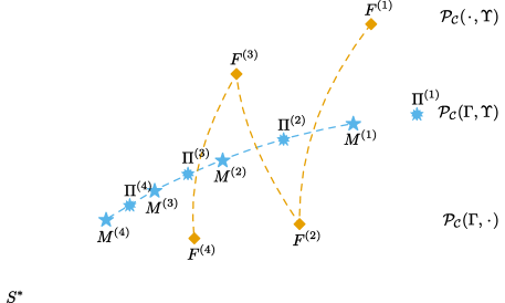
Figure 1: Conceptual representation of IPF and IDBM iterations (inspired by Figure 1 of Bernton et al. (2019)), the ordering of $Π^{(i)}$ and $M^{(i)}$ is justified by Theorem 2.

Theorem 2 (IDBM convergence)

For $Γ,ϒ∈𝒫_{1}$, $R∈𝒫_{𝒞}$ associated to 3 with $σ_{R}(x,t)=I$, consider the iterates $Π^{(i)},M^{(i)}∈𝒫_{𝒞}(Γ,ϒ)$ of Algorithm 2. Assume that: (i) $D_{KL}(C^{(0)}\mathbin{\textbardbl}S^{*}_{0,τ})<∞$; (ii) for each $i≥1$ the Cameron-Martin-Girsanov theorem hold for $M^{(i)}$ yielding $dM^{(i)}/dS^{*}$ (implying that 24 for $Π=Π^{(i)}$ has a unique diffusion solution with law $M^{(i)}$, and that $M^{(i)}≪S^{*}$). Then: (i) $Π^{(i)}\overset{ℒ}{⟶}S^{*}$ and $M^{(i)}\overset{ℒ}{⟶}S^{*}$ as $i\textrightarrow∞$, where $\overset{ℒ}{⟶}$ denotes converge in law; (ii) $D_{KL}(Π^{(i)}\mathbin{\textbardbl}S^{*})≥D_{KL}(M^{(i)}\mathbin{\textbardbl}S^{*})≥D_{KL}(Π^{(i+1)}\mathbin{\textbardbl}S^{*})$ for $i≥1$ (implying that $D_{KL}(M^{(i)}\mathbin{\textbardbl}S^{*})$ is non-increasing in $i$); (iii) $D_{KL}(Π(C)\mathbin{\textbardbl}S^{*})=D_{KL}(M(C)\mathbin{\textbardbl}S^{*})$ if and only if $Π(C)=M(C)=S^{*}$.

In generative modeling applications, the simplest choice is to set $C^{(0)}$ to the independent coupling $Γ{⊗}ϒ$, from which samples are trivially obtainable. Dependent couplings are the natural choice in other applications. In inverse problems, $C^{(0)}$ would be the distribution of pairs of clean and corrupted (or latent and partially observed) data. Applications of the DBM transport to inverse problems and to aligned data are reviewed in Section 5. We briefly consider dependent initial couplings in Section 6.1.

We still need to address the problem of inferring the drift coefficients of 24 or 26 for each iteration $i$ of Algorithm 2. The projection property of conditional expectations once again yields suitable objectives for the drift adjustments:

$$𝔼_{Π}[Σ_{R}(X_{t},t)∇_{X_{t}}\log r_{τ|t}(X_{τ}|X_{t})|X_{t}=x]=\operatorname*{arg\,min}_{α(x,t)}𝕃_{\mathrm{DBM}}(α,Π,R,Σ_{R}),$$ (27)

$$𝕃_{\mathrm{DBM}}(α,Π,R,Σ_{R})≔𝔼_{t∼𝒰(0,τ)}[ϱ_{t}𝔼_{Π}[\textbardbl α(X_{t},t)-Σ_{R}(X_{t},t)∇_{X_{t}}\log r_{τ|t}(X_{τ}|X_{t})\textbardbl^{2}]],$$

$$𝔼_{Π}[Σ_{R}(X_{t},t)∇_{X_{t}}\log r_{t|0}(X_{t}|X_{0})|X_{t}=x]=\operatorname*{arg\,min}_{α(x,t)}𝕃_{\mathrm{BDBM}}(α,Π,R,Σ_{R}),$$

$$𝕃_{\mathrm{BDBM}}(α,Π,R,Σ_{R})≔𝔼_{t∼𝒰(0,τ)}[λ_{t}𝔼_{Π}[\textbardbl α(X_{t},t)-Σ_{R}(X_{t},t)∇_{X_{t}}\log r_{t|0}(X_{t}|X_{0})\textbardbl^{2}]].$$

In 27, $ϱ_{t}:(0,τ)\textrightarrow ℝ_{>0}$ and $λ_{t}:(0,τ)\textrightarrow ℝ_{>0}$ are time-dependent regularizers that compensates for the diverging $∇_{x}\log r_{τ|t}(y|x)$ as $t\textrightarrow τ$ and $∇_{y}\log r_{t|0}(y|x)$ as $t\textrightarrow 0$.

Although we rely exclusively on 27 in the numerical experiments of Section 6, we can leverage additional inferential objectives. Indeed, under mild conditions, performing inference following the description in Section 2.4 on data simulated from $Π$ allows the recovery of the drift coefficients $μ_{M}(x,t)$ and $υ_{M}(x,t)$. For instance, plugging-in the representation 25 in 12 yields $μ_{M}(x,t)=\operatorname*{arg\,max}_{α(x,t)}𝕆_{\mathrm{MLE}}(α,Π,Σ_{R})$, while that $μ_{M}(x,t)≈\operatorname*{arg\,min}_{α(x,t)}𝕃_{\mathrm{DM}}(α,Π,Δt)$ follows directly from the definition of $Π$ by interchanging limits. Proofs are omitted here.

We take a moment to provide several comments on the proposed IDBM procedure, contrasting it with the IPF procedure detailed in Section 2.3:

1. the IPF iterations generate a sequence of initial-terminal measures $F^{(i)}_{0,τ}∈𝒫_{2}(Γ,□)∪𝒫_{2}(□,ϒ)$ that matches one of the target marginal distributions $Γ$, $ϒ$ at a time, thus producing a valid coupling between $Γ$ and $ϒ$ only in the limit where $(\mathrm{S_{sta}})$ is solved; in contrast, each IDBM iteration produces a valid initial-terminal coupling $C^{(i)}∈𝒫_{2}(Γ,ϒ)$, with the sequence of coupling being progressively optimal toward solving $(\mathrm{S_{sta}})$; this crucial difference is depicted in the sketch of Figure 1;

2. IPF iterations necessarily alternates between forward and backward time directions; each IDBM iterations can be solved in either of the time direction (or both);

3. approaches relying on samples from $F^{(i-1)}$ to infer the drift coefficient of $F^{(i)}$ suffer from the simulation-inference distribution mismatch $\overline{F}^{(i-1)}≠F^{(i)}$ which can negatively impact inferential efficiency; by construction $Π^{(i)}$ and $M^{(i)}$ share the same marginal distributions, so samples from $Π^{(i)}$ are guaranteed to cover regions of high probability according to $M^{(i)}$, thus making inference of the corresponding drift coefficient reliable;

4. the measures resulting from the IPF iterations do not admit a simple marginal-conditional decomposition; in contrast each $Π^{(i)}$ is given by a mixture of diffusion bridges.

The aforementioned points suggest that using the IDBM can be advantageous within the context of generative models. Point (i) establishes that truncating the IDBM iterations at a finite iteration number does not bias the transport. Even the first iteration of the IDBM procedure produces a valid, even if suboptimal, transport. In Section 6.3 we follow this program as an alternative to the SGM approach. In contrast, the IPF procedure requires employing many iterations, which can be computationally expensive. Nevertheless, when multiple IDBM iterations are desirable, it might prove beneficial to solve the iterations alternating between the forward and backward time directions. As the approximation and discretization errors cumulate over the iterates, repeatedly solving the IDBM procedure in the same time direction could lead to a terminal distribution progressively deviating from the corresponding target marginal distribution. Points (iii) and (iv) point to potential efficiency gains of the IDBM procedure. Indeed, at iteration $i>1$, inferring the drift coefficients of both the IPF and the IDBM requires the numerical discretization and simulation from an SDE associated to iteration $i-1$. This is computationally expensive: in Bortoli et al. (2021) paths are sampled, cached, and re-used for 100 steps of gradient descent. With this choice, path sampling still amounts to roughly $50\%$ of the total computational time. In the IDBM procedure, simulated paths, which are similarly costly to produce, give raise to samples from $C^{(i-1)}$. However, this time, each sample from $C^{(i-1)}$ can be used to generate multiple samples at arbitrary time points from $Π^{(i)}=C^{(i-1)}R_{\textbullet|0,τ}$ which, for SDEs typically used in generative modeling (Section 4), can be done inexpensively and exactly (see 32). We implement this approach in the empirical comparison of Section 6.4.

4 Reference SDE Class

In this section we introduce a class of reference SDEs. This is achieved in two steps: first we formulate a simple SDE, 28, then we show that SDEs commonly employed in generative models such as Song et al. (2021), i.e. SDE 33, are realized through a time change.

Consider the $d$-dimensional linear SDE

$$dY_{t}=-αY_{t}dt+Σ^{1/2}dW_{t},\quad t≥0,$$ (28)

$$Y_{0}∼Γ,$$

with associated path PM $P$, where $α≥0$ is a scalar and $Σ$ is a positive definite covariance matrix. For $α=0$, 28 yields a correlated and scaled Brownian motion, otherwise 28 corresponds to an Ornstein-Uhlenbeck process. For $α=\frac{1}{2}$, 28 has stationary distribution $𝒩_{d}(0,Σ)$. The transition densities $p_{t|s}$ of 28 are Gaussian:

$$(Y_{t}|Y_{s})∼𝒩_{d}(Y_{s}a(s,t),Σv(s,t)),$$ (29)

$$a(s,t)=e^{-α(t-s)},$$

$$v(s,t)=\begin{cases*}t-s,&if $α=0$,\\ \frac{1}{2α}(1-e^{-2α(t-s)}),&if $α>0$,\end{cases*}$$

and

$$∇_{y_{s}}\log p_{t|s}(y_{t}|y_{s})=Σ^{-1}\bigg{(}\frac{y_{t}}{a(s,t)}-y_{s}\bigg{)}\frac{a^{2}(s,t)}{v(s,t)},$$ (30)

$$∇_{y_{t}}\log p_{t|s}(y_{t}|y_{s})=Σ^{-1}\bigg{(}y_{s}a(s,t)-y_{t}\bigg{)}\frac{1}{v(s,t)},$$ (31)

which shows that the diffusion bridge 17 corresponding to 28 remains a linear SDE. From Bayes theorem and the Markov property, for $0≤s<t<u$,

$$(Y_{t}|Y_{s},Y_{u})∼𝒩_{d}(Y_{s}\hat{a}(s,t,u)+Y_{u}\check{a}(s,t,u),\,Σ\tilde{v}(s,t,u)),$$ (32)

$$\hat{a}(s,t,u)=\frac{v(t,u)a(s,t)}{v(s,t)a^{2}(t,u)+v(t,u)},$$

$$\check{a}(s,t,u)=\frac{v(s,t)a(t,u)}{v(s,t)a^{2}(t,u)+v(t,u)},$$

$$\tilde{v}(s,t,u)=\frac{v(s,t)v(t,u)}{v(s,t)a^{2}(t,u)+v(t,u)}.$$

We consider the following time change of 28. Let $β_{t}:[0,τ]\textrightarrow ℝ_{>0}$ be a continuous strictly positive function and $b_{t}≔∫_{0}^{t}β_{u}du$. Then $b_{t}:[0,τ]\textrightarrow[0,b_{τ}]$ is differentiable strictly increasing function and $β_{t}=\frac{db_{t}}{dt}$. An application of (Øksendal, 2003, Theorem 8.5.1) establishes that the time-changed process $X_{t}≔Y_{b_{t}}$ is equivalent in law to the solution to

$$dX_{t}=-αβ_{t}X_{t}dt+\sqrt{β_{t}}Σ^{1/2}dW_{t},\quad t∈[0,τ],$$ (33)

$$X_{0}∼Γ.$$

That is, SDE 33 corresponds to the evolution of the simpler SDE 28 under a non-linear time wrapping where time flows with instantaneous intensity $β_{t}$.

We conclude this section by specializing 16, 24 and 26 to the case of a reference SDE given by $dX_{t}=σdW_{t}$, $σ>0$, referring to Appendix B for the general setting. The generative time reversal process 16 is given by

$$d\overline{X}_{t}=\frac{𝔼_{R}[\overline{X}_{τ}|\overline{X}_{t}]-\overline{X}_{t}}{τ-t}dt+σdW_{t},\quad t∈[0,τ],$$

$$\overline{X}_{0}∼ϒ.$$

The DBM transport 24 is given by

$$dX_{t}=\frac{𝔼_{Π}[X_{τ}|X_{t}]-X_{t}}{τ-t}dt+σdW_{t},\quad t∈[0,τ],$$ (34)

$$X_{0}∼Γ,$$

while the BDBM transport 26 is given by

$$d\overline{X}_{t}=\frac{𝔼_{Π}[\overline{X}_{τ}|\overline{X}_{t}]-\overline{X}_{t}}{τ-t}dt+σdW_{t},\quad t∈[0,τ],$$ (35)

$$\overline{X}_{0}∼ϒ.$$

In this case the DBM and BDBM transports are symmetric: the BDM transport based on $C∈𝒫_{2}(Γ,ϒ)$ is equivalent in law to the BDBM transport based on $\overline{C}∈𝒫_{2}(ϒ,Γ)$.

5 Additional Related Literature

The DBM transport is initially introduced in the unpublished manuscript (Peluchetti, 2021), which, however, lacks empirical validations. This shortcoming is subsequently addressed by Wu et al. (2022); Liu et al. (2023b), who successfully implements the DBM transport across a multitude of applications, among other significant contributions. Liu et al. (2023b) demonstrates that the DBM transport corresponds to an optimal Markovianization of the mixture of diffusion bridges it matches. The theoretical developments associated with this finding contribute to our proof of Theorem 2. The proposal put forth by Liu et al. (2023a) is equivalent to the DBM transport for a reference scaled Brownian motion, and its application is shown to yield competitive results in image restoration problems. Similarly, the proposal of Somnath et al. (2023) is equivalent to the DBM for the same reference dynamics. It also assumes that the initial coupling is optimal, and thus preserved. The resulting methodology is successfully applied to the case of aligned data. While both works are equivalent to a specific instance of the DBM transport, they differ in certain aspects of implementation, such as the choice of the discretization scheme for sampling SDE paths and the definition of the loss regularizer. These studies further substantiate the satisfactory performance we observe in the dataset transfer experiment of Section 6.4 for the BDBM transport.

Concurrently and independently of our research, Shi et al. (2023) introduces the Diffusion Schrödinger Bridge Matching—Iterative Markovian Fitting (DSBM-IMF) procedure, which is equivalent to the IDBM procedure developed in this work. Shi et al. (2023) conducts a preliminary theoretical assessment of the convergence properties of the DSBM-IMF procedure and empirically compares it with the proposal of Bortoli et al. (2021). One of the numerical experiments pertains to the Gaussian setting detailed in Section 6.1, with $Σ_{0}=Σ_{1}=I$ and $d=50$. In contrast to our investigation, neural networks approximators are utilized and trained iteratively. The subsequent results are consistent with our findings of Section 6.1.

The Rectified Flow (RF) method, introduced in Liu et al. (2022) and further explored in Liu (2022), is particularly pertinent to the IDBM procedure discussed in this paper due to their significant similarities. The RF procedure commences with an initial coupling $C∈𝒫_{2}(Γ,ϒ)$, from which it constructs a mixing process, denoted as $Φ≔CL_{\textbullet|0,1}$, via the deterministic linear interpolant process $L_{\textbullet|0,1}$. The latter is defined by $X_{t}≔(1-t)X_{0}+tX_{1}$, where $t∈[0,1]$. A rectification of this mixing process is then introduced, given by the solution to the RF ODE

$$dV_{t}=ν(V_{t},t)dt,\quad t∈[0,1],$$

$$V_{0}∼Γ,$$

where $ν(x,t)≔𝔼_{Φ}[X_{1}-X_{0}|X_{t}=x]$.

It is shown in Liu et al. (2022) that this rectification procedure results in a valid coupling: $\mathrm{Law}(V_{0},V_{1})∈𝒫_{2}(Γ,ϒ)$. Moreover, when the rectification process is iterated, it yields a sequence of couplings, $\mathrm{Law}(V^{(i)}_{0},V^{(i)}_{1})$, where $i≥1$, such that $𝔼[κ(V^{(i)}_{1}-V^{(i)}_{0})]$ is non-increasing across all convex cost functions $κ:ℝ^{d}\textrightarrow ℝ$. For additional properties of the RF procedure, we direct the reader to Liu et al. (2022). Finally, Liu (2022) establishes that while the RF method successfully solves the one-dimensional Euclidean OT problem, it does not address the multidimensional variant. Consequently, a modification of the RF approach is introduced, which is proven to effectively solve the multidimensional Euclidean OT problem.

The RF method can be understood as the limiting case of the IDBM procedure for a reference scaled Brownian motion as its randomness vanishes. Indeed, consider the reference measure $R$ associated to $dX_{t}=σdW_{t}$ over $t∈[0,1]$. $X_{t}∼R_{t|0,1}$ is realized by $X_{t}=(1-t)X_{0}+tX_{1}+σ\sqrt{t(1-t)}Z_{t}$, where $Z_{t}∼N(0,1)$. The DBM drift is given by

$$μ_{M}(x,t)=𝔼_{Π}\Big{[}\frac{X_{1}-X_{t}}{1-t}\mathrel{\Big{|}}X_{t}=x\Big{]}=𝔼_{Π}\Big{[}X_{1}-X_{0}-σ\sqrt{\frac{t}{1-t}}Z_{t}\mathrel{\Big{|}}X_{t}=x\Big{]},$$

for $Π=CR_{\textbullet|0,1}$. As $σ\textrightarrow 0$ the Brownian bridge’s marginal variances converge to zero, while its marginal means are independent of $σ$. Informally, $Π\textrightarrow Φ$ and we obtain the aforementioned limiting equivalence. Section 6.1 expands on this connection within a fully Gaussian setting. Moreover, the conclusions drawn from the numerical experiment of Section 6.4 indicate that the optimal value of $σ$ depends on the specific application. In particular, our attempts to apply the RF procedure to this dataset transfer experiment have not yielded satisfactory results.

As shown in Shi et al. (2023), under certain conditions, both the Flow Matching (FM) proposed by Lipman et al. (2023) and the Conditional Flow Matching (CFM) suggested by Tong et al. (2023) correspond to the first iteration of the RF for generative modeling with a standard Gaussian as the initial distribution. The OT-CFM variant, as introduced by Tong et al. (2023), initially attempts to solve the EOT problem to derive an optimal coupling, followed by fitting a stochastic process to preserve this optimal coupling. This approach is analogous to computing the DBM transport starting from the optimal coupling.

Finally, Chen et al. (2022), while sharing similarities with the work of Bortoli et al. (2021); Vargas et al. (2021), introduces divergence-based objectives, while Thornton et al. (2022) extends the scope of the DIPF method of (Bortoli et al., 2021) by generalizing it to non-Euclidean settings.

6 Applications

In this section we consider four applications of the IDBM procedure.

6.1 Gaussian Transports

We investigate in depth the case where both the initial and terminal distributions are $d$-dimensional Gaussian distributions, $Γ=𝒩_{d}(μ_{0},Σ_{0})$, $ϒ=𝒩_{d}(μ_{1},Σ_{1})$, and the reference measure $R$ is associated to $dX_{t}=σdW_{t}$ over the time interval $[0,1]$. The solution to the Euclidean EOT problem, or to $(\mathrm{S_{sta}})$, defined by $(Γ,ϒ,R)$, is the Gaussian coupling

$$S^{*}_{0,1}(Γ,ϒ,R,𝒫_{𝒞})=𝒩_{2d}\left(\begin{bmatrix}μ_{0}\\ μ_{1}\end{bmatrix},\begin{bmatrix}Σ_{0}&Σ_{S}(σ)\\ Σ_{S}(σ)ᵀ&Σ_{1}\end{bmatrix}\right),$$ (36)

where $Σ_{S}(σ)≔(Σ_{0}Σ_{1}+\frac{σ^{4}}{4}I)^{1/2}-\frac{σ^{2}}{2}I$. The solution $OT^{*}(Γ,ϒ)$ to the OT problem is obtained setting $σ=0$ in 36, with corresponding OT plan $φ_{OT}(x)≔μ_{1}+Σ_{0}^{-1}Σ_{S}(0)(x-μ_{0})$. See for instance Peyré and Cuturi (2020, Section 2.6) and Janati et al. (2020, Section 2).

Consider the DBM transport based on the Gaussian coupling $C∈𝒫_{2}(Γ,ϒ)$,

$$C=𝒩_{2d}\left(\begin{bmatrix}μ_{0}\\ μ_{1}\end{bmatrix},\begin{bmatrix}Σ_{0}&Σ_{C}\\ Σ_{C}ᵀ&Σ_{1}\end{bmatrix}\right).$$ (37)

The mixture of diffusion bridges with law $Π(C,R_{\textbullet|0,1})$ has a joint distribution $Π_{0,t,1}(C,R_{\textbullet|0,1})$ which is again Gaussian,

$$Π_{0,t,1}(C,R_{\textbullet|0,1})=𝒩_{3d}\left(\begin{bmatrix}μ_{0}\\ (1-t)μ_{0}+tμ_{1}\\ μ_{1}\end{bmatrix},\begin{bmatrix}Σ_{0}&Σ_{Π;0,t}&Σ_{C}\\ Σ_{Π;0,t}ᵀ&Σ_{Π;t,t}&Σ_{Π;t,1}\\ Σ_{C}ᵀ&Σ_{Π;t,1}ᵀ&Σ_{1}\end{bmatrix}\right),$$

where $Σ_{Π;0,t}≔(1-t)Σ_{0}+tΣ_{C}$, $Σ_{Π;t,t}≔(1-t)^{2}Σ_{0}+t^{2}Σ_{1}+t(1-t)(Σ_{C}+Σ_{C}ᵀ+σ^{2}I)$ and $Σ_{Π;t,1}≔(1-t)Σ_{C}+tΣ_{1}$. It follows that

$$𝔼_{Π}[X_{1}|X_{t}]=μ_{1}+Σ_{Π;t,1}ᵀΣ_{Π;t,t}^{-1}(X_{t}-μ_{t})$$

and thus the DBM transport with law $M(Π(C,R_{\textbullet|0,1}))$ is given by the solution to

$$dX_{t}=\frac{𝔼_{Π}[X_{1}|X_{t}]-X_{t}}{1-t}dt+σdW_{t},\quad t∈[0,1],$$ (38)

$$X_{0}∼Γ.$$

SDE 38 is of the form $dX_{t}=(A_{t}X_{t}+b_{t})dt+σdW_{t}$ for $A_{t}:[0,1]\textrightarrow ℝ^{d×d}$, $b_{t}:[0,1]\textrightarrow ℝ^{d}$, i.e. it is linear and time-inhomogenous with Gaussian transition probabilities. The following representation holds: $X_{1}|X_{0}$ is distributed as $P_{1}X_{0}+ε$, where $P_{t}$ is given by the solution to the matrix-valued ODE

$$dP_{t}=A_{t}P_{t},\quad t∈[0,1],$$ (39)

$$P_{0}=I,$$

and $ε$ is a $d$-dimensional Gaussian distribution whose parameters depend on the functions $A_{t}$ and $b_{t}$, but not on $X_{0}$. In conclusion,

$$M_{0,1}(Π(C,R_{\textbullet|0,1}))=𝒩_{2d}\left(\begin{bmatrix}μ_{0}\\ μ_{1}\end{bmatrix},\begin{bmatrix}Σ_{0}&Σ_{C^{\prime}}\\ Σ_{C^{\prime}}ᵀ&Σ_{1}\end{bmatrix}\right),\quad Σ_{C^{\prime}}≔Σ_{0}P_{1}ᵀ.$$ (40)

Starting from the Gaussian coupling $C^{(0)}=Γ{⊗}ϒ$, i.e. $Σ_{C^{(0)}}=0I$, the IDBM procedure iteratively computes the updates $Σ_{C}\textrightarrow Σ_{C^{\prime}}$ resulting in a sequence of Gaussian couplings $C^{(i)}$.

The IPF updates for $(\mathrm{S_{sta}})$ can be computed analytically thanks to the following property of Gaussian distributions. Let $X$ and $Y$ be $d$-dimensional random variables with $(X,Y)∼P_{X,Y}$, where

$$P_{X,Y}≔𝒩_{2d}\left(\begin{bmatrix}μ_{x}\\ μ_{y}\end{bmatrix},\begin{bmatrix}Σ_{xx}&Σ_{xy}\\ Σ_{xy}ᵀ&Σ_{yy}\end{bmatrix}\right),$$

and denote with $P_{Y|X}$ the conditional distribution of $Y$ given $X$ under $P_{X,Y}$. For $Q_{X}≔𝒩_{d}(λ_{x},Γ_{xx})$, we have

$$Q_{X}P_{Y|X}=𝒩_{2d}\left(\begin{bmatrix}λ_{x}\\ λ_{y}\end{bmatrix},\begin{bmatrix}Γ_{xx}&Γ_{xy}\\ Γ_{xy}ᵀ&Γ_{yy}\end{bmatrix}\right),$$ (41)

$$λ_{y}≔μ_{y}+Σ_{xy}ᵀΣ_{xx}^{-1}(λ_{x}-μ_{x}),$$

$$Γ_{xy}≔Γ_{xx}Σ_{xx}^{-1}Σ_{xy},$$

$$Γ_{yy}≔Σ_{yy}+Σ_{xy}ᵀ(Σ_{xx}^{-1}Γ_{xx}Σ_{xx}^{-1}-Σ_{xx}^{-1})Σ_{xy}.$$

Therefore, starting from

$$F^{(0)}_{0,1}=𝒩_{2d}\left(\begin{bmatrix}μ_{0}\\ μ_{0}\end{bmatrix},\begin{bmatrix}Σ_{0}&Σ_{0}\\ Σ_{0}&Σ_{0}+σ^{2}I\end{bmatrix}\right),$$

the IPF iterations update one of the marginal distributions of $F^{(i)}_{0,1}$ at a time via 41.

When $d=1$, ODE 39 can be solved analytically. The coupling distribution 37 has a single degree of freedom, its correlation coefficient, which we denote with $ρ_{C}$. Then, $M_{0,1}(Π(C,R_{\textbullet|0,1}))∈𝒫_{2}(Γ,ϒ)$ is Gaussian with correlation coefficient

$$ρ_{M}(ρ_{C},Σ_{0},Σ_{1},σ)≔\exp\left\{-σ^{2}\frac{\tanh^{-1}(\frac{c_{1}}{c_{3}})+\tanh^{-1}(\frac{c_{2}}{c_{3}})}{c_{3}}\right\}$$ (42)

$$c_{1}=σ^{2}+2Σ_{1}(ρ_{C}Σ_{0}-Σ_{1}),c_{3}=\sqrt{(σ^{2}+2(ρ_{C}+1)Σ_{0}Σ_{1})(σ^{2}+2(ρ_{C}-1)Σ_{0}Σ_{1})},$$

$$c_{2}=σ^{2}+2Σ_{0}(ρ_{C}Σ_{1}-Σ_{0}),$$

which is independent of $μ_{0},μ_{1}$. The following results hold: (i) for fixed $σ,Σ_{0},Σ_{1}$, the map $ρ_{M}(ρ,Σ_{0},Σ_{1},σ):ρ↦ρ^{\prime}$ is a contraction over $ρ∈[-1,1]$ with limiting value $(\sqrt{Σ_{0}Σ_{1}+\frac{σ^{4}}{4}}-\frac{σ^{2}}{2})/\sqrt{Σ_{0}Σ_{1}}$, i.e. the correlation coefficient of $S^{*}_{0,1}(Γ,ϒ,R,𝒫_{𝒞})$; (ii) for fixed $ρ,Σ_{0},Σ_{1}$, $\lim_{σ->0}ρ_{M}(ρ,Σ_{0},Σ_{1},σ)=ρ_{M}(ρ,Σ_{0},Σ_{1},0)=1$, i.e. the correlation coefficient of $OT^{*}(Γ,ϒ)$. Result (i) establishes that the couplings produced by the IDBM iterations converge to $S^{*}_{0,1}(Γ,ϒ,R,𝒫_{C})$, as expected from Theorem 2. Result (ii) shows that the DBM transport remains well-posed for vanishing regularization $σ$, and that $M^{(1)}_{0,1}\overset{ℒ}{⟶}OT^{*}(Γ,ϒ)$ as $σ\textrightarrow 0$, i.e. convergence (in law) is attained by the first iteration of the IDBM procedure. For further insight, reconsider the DBM SDE $dX_{t}=(A_{t}X_{t}+b_{t})dt+σdW_{t}$. In the noiseless limit $σ\textrightarrow 0$, the dynamics are specified by the DBM ODE $dx_{t}=(A^{0}_{t}x_{t}+b^{0}_{t})dt$, which corresponds to the RF ODE (Section 5), where $A^{0}_{t}≔\lim_{σ\textrightarrow 0}A_{t}$ and $b^{0}_{t}≔\lim_{σ\textrightarrow 0}b_{t}$. Moreover, the solution $M$ to the DBM SDE converges in law to the solution to the DBM ODE (Stroock and Varadhan, 2006, Chapter 11). Solving the DBM ODE and computing the solution at terminal time yields $x_{1}=μ_{1}+\sqrt{Σ_{1}/Σ_{0}}(x_{0}-μ_{0})=φ_{OT}(x_{0})$, the OT plan.

	$\lim$ $D_{KL}(M^{(1)}_{0,1}\mathbin{\textbardbl}S^{*}_{0,1})$ $D_{KL}(F^{(1)}_{0,1}\mathbin{\textbardbl}S^{*}_{0,1})$ $μ_{\{0,1\}}\textrightarrow\pm∞$ $k$ $∞$ $Σ_{\{0,1\}}\textrightarrow∞$ $K_{Π}$ $∞$ $Σ_{\{0,1\}}\textrightarrow 0$ $0$ $k$ $σ\textrightarrow∞$ $0$ $0$ $σ\textrightarrow 0$ $k$ $∞$
Figure 2: Convergence of IPF and IDBM initial-terminal PMs to $S^{*}_{0,1}$ in KL divergence; $d=1$; log-scale.	Table 1: Summary of limiting behavior of the first iteration of the IDBM and IPF procedures; $d=1$.

We consider the scenario $μ_{0}=-1,μ_{1}=1,Σ_{0}=Σ_{1}=σ^{2}=1$. We compute the KL divergence from the IPF PMs $F^{(i)}_{0,1}$ and from the IDBM couplings $M^{(i)}_{0,1}$ to $S^{*}_{0,1}(Γ,ϒ,R,𝒫_{𝒞})$ as function of the iterations. The KL divergence between multivariate Gaussian distributions can be calculated analytically, so no approximation is required. The results are shown in Figure 2 where, in addition to the standard initial independent coupling $C^{(0)}=Γ{⊗}ϒ$, we consider two additional initial couplings with correlations $ρ_{C^{(0)}}=\pm 1$. It is observed that the IDBM iterations exhibit a higher rate of convergence with respect to the KL divergence. We note that with our choice of indexing, we slightly favor the IPF iterations, as $F^{(0)}_{0,1}$ already incorporates the reference measure $R$, while $C^{(0)}$ does not depend on $R$.

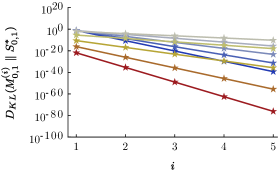
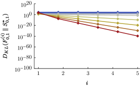
Figure 3: Same as Figure 2 for varying levels of regularization $σ$; (left): IDBM; (right): IPF; $d=1$; shared log-scale.

In Figure 3 we modify the considered scenario by varying the level of regularization: $σ=10^{s}$ for $s=-2,…,2$, with $σ=10^{-2}$ corresponding to the blue color and $σ=10^{2}$ to the red color. While the IDBM iterations converge quickly for both low and high levels of regularization (with $σ=1$, as in Figure 2, exhibiting the slowest convergence), the IPF iterations display increasing KL divergence for vanishing $σ$.

We complete the analysis of the one-dimensional setting by studying the behavior of $D_{KL}(M^{(1)}_{0,1}\mathbin{\textbardbl}S^{*}_{0,1})$ and $D_{KL}(F^{(1)}_{0,1}\mathbin{\textbardbl}S^{*}_{0,1})$ at the boundaries of the parameters’ space spanned by $θ=(μ_{0},μ_{1},Σ_{0},Σ_{1},σ)$. The results are reported in Table 1, where $k$ denotes positive finite values, $K_{Π}≔\frac{1}{4}(π+\log[4]-2(1+\log[π]))$ is the supremum of $D_{KL}(M^{(1)}_{0,1}\mathbin{\textbardbl}S^{*}_{0,1})$ over $θ$, $μ_{\{0,1\}}$ stands for either of $μ_{0}$, $μ_{1}$, and $Σ_{\{0,1\}}$ stands for either of $Σ_{0}$, $Σ_{1}$. When taking each limit all other parameters are kept constant. Note that all of $M^{(1)}_{0,1}$, $F^{(1)}_{0,1}$ and $S^{*}_{0,1}$ depend on $θ$, even though the notation does not make this explicit. The results of Table 1 support the robustness of the IDBM procedure in the one-dimensional setting. In particular, the IDBM procedure does not suffer from the difficulties in bridging distant distributions which are inherent to DIPF approaches (Vargas et al., 2021).

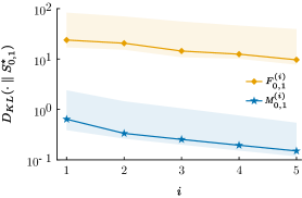
Figure 4: Convergence of IPF and IDBM initial-terminal PMs to $S^{*}_{0,1}$ in KL divergence; (left): $d=5$; (right): $d=10$; log-scale.

For $d>1$, we numerically integrate the matrix-valued ODE 39. We generate $20$ scenarios for each of $d=5,10$. In each scenario, we sample $μ_{0},μ_{1}$ uniformly on $[-1,1]^{d}$ and $Σ_{0},Σ_{1}$ from a Wishart distribution with $d$ degrees of freedom and covariance matrix $0.2I$ (as in Janati et al. (2020)). We set $σ=0.2$ when $d=5$ and $σ=1$ when $d=10$. In the multivariate instance, $M^{(1)}_{0,1}$ does not converge to $OT^{*}(Γ,ϒ)$ as $σ\textrightarrow 0$, and the convergence rate of the IDBM procedure worsens as $σ$ approaches $0$. Indeed, in the Gaussian setting defined for this study, the $σ\textrightarrow 0$ limit of the DBM transport is equivalent to the RF of Liu et al. (2022) (Section 5), and Liu (2022) establishes that the RF solves the OT problem only in the one-dimensional case. Nonetheless, the IDBM procedure consistently outperforms the IPF procedure in all scenarios. In Figure 4 we plot the average KL divergences from $M^{(i)}_{0,1}$ and from $F^{(i)}_{0,1}$ to $S^{*}_{0,1}$ as function of the iterations with solid lines, where each average is over the $20$ sampled scenarios. The banded regions correspond to the ranges between the highest and the lowest KL divergence values across the scenarios.

6.2 Mixture Transports

We consider $Γ=\frac{1}{3}(𝒩_{1}(-3,0.2^{2})+𝒩_{1}(0.5,0.2^{2})+𝒩_{1}(3,0.2^{2}))$, $ϒ=𝒩_{1}(0,2^{2})$, and $R$ associated to $dX_{t}=σdW_{t}$ over the time interval $[0,1]$ for $σ=0.2$. This configuration is selected to illustrate the limitation of the sampling-based DIPF procedures discussed in Section 2.3.

The goal of this application is to construct a transport from $ϒ$ to $Γ$. This toy experiment can be seen as a simplified instance of the generative setting introduced in Section 2.5, where the training data consist of the values $-3,0.5,3$ and $Γ=D_{η}$ for $η=0.2$. Compared with typical applications, $σ$ has been set to a small value to introduce a strong dependency between $X_{0}$ and $X_{1}$ under $R$, making SGM approaches inapplicable.

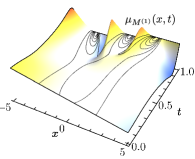
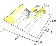
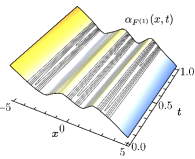
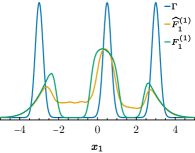
Figure 5: Drift (left), estimated drift (center) and terminal density (right) resulting from the first iteration of the IPF (bottom) and IDBM (top) procedures; generative time.

In this application, we always assume time $t$ on the generative timescale. The first iteration of the IPF procedure relies on samples from $R$ to infer $μ_{F^{(1)}}(x,t)$. We display $μ_{F^{(1)}}(x,t)$ in Figure 5 (bottom-left), superimposed with gray lines representing the level sets of the marginal densities $r_{t}$, $t∈[0,1]$. Samples from $R$ have negligible probability of falling outside narrowly defined regions. We employ as drift approximator a fully-connected neural network $α(θ,x,t)$ with 3 hidden layers, the ReLU ($x\textrightarrow\max(0,x)$) activation function, and a width of $512$ units. Utilizing objective 14, $α(θ,x,t)$ is optimized via stochastic gradient descent (SGD). We display the resulting inferred drift coefficient at convergence, $α_{F^{(1)}}(x,t)$, in Figure 5 (bottom-center). Again we superimpose with the level sets of $r_{t}$. The approximation is accurate in regions of high probability under $R$, but significantly deteriorates outside these regions. We contrast the true density of $F^{(1)}_{1}$ with a kernel density estimate based on 10 million samples from $\widehat{F}_{1}^{(1)}$, which are obtained by applying the Euler scheme, $Δt=10^{-4}$, to

$$dX_{t}=α_{F^{(1)}}(X_{t},t)dt+σdW_{t},\quad t∈[0,1],$$

$$X_{0}∼ϒ,$$

and collecting the terminal states. As illustrated in Figure 5 (bottom-right), the approximation errors have a significant impact.

Implementing sampling-based DIPF procedures requires carefully tuning the level of regularization. On the one hand, an excessively high level of $σ$ renders IPF iterations after the first superfluous, with $F^{(1)}$ already approximately solving $(\mathrm{S_{dyn}})$. On the other hand, an excessively low level of $σ$ risks incurring the difficulties just exposed. We remark that, in particular instances, the simulation-inference mismatch can become irrelevant. This is the case for the Gaussian transports of Section 6.1, where $F^{(i)}_{t}$ is a multivariate Gaussian distribution for each $i$ and $t$ (Mallasto et al., 2022). Therefore, $μ_{F^{(i)}}(x,t)$ is an affine function in $x$ for each $i$ and $t$, in which case local information about $μ_{F^{(i)}}(x,t)$ is global as well.

We construct the IDBM procedure started from $C^{(0)}=ϒ{⊗}Γ$. The drift coefficient $μ_{M^{(1)}}(x,t)$ corresponding to the first IDBM iteration is illustrated in Figure 5 (top-left), superimposed with gray lines representing the level sets of the marginal densities $π^{(1)}_{t}$, $t∈[0,1]$. Drift inference is based on samples from $Π^{(1)}$. The same neural network architecture is employed, and utilizing objective 27 $α(θ,x,t)$ is optimized via SGD. We display the resulting inferred drift coefficient at convergence $α_{M^{(1)}}(x,t)$ in Figure 5 (top-center), superimposing the level sets of $π^{(1)}_{t}=m^{(1)}_{t}$. As expected, $α_{M^{(1)}}(x,t)$ closely approximates $μ_{M^{(1)}}(x,t)$ in regions of high probability under $Π^{(1)}$. Crucially, this suffices for learning $μ_{M^{(1)}}(x,t)$ on the regions of the path space relevant for the simulation from $M^{(1)}$. An interesting observation is that the drift coefficient $μ_{M^{(1)}}(x,t)$ is smoother than $μ_{F^{(1)}}(x,t)$. This aspect makes it easier to both approximate $μ_{M^{(1)}}(x,t)$ with a neural network and accurately simulate from the resulting SDE. We contrast the true density of $Γ$ with a kernel density estimate based on 10 million samples from $\widehat{M}_{1}^{(1)}$, which are obtained by applying the Euler scheme, $Δt=10^{-4}$, to

$$dX_{t}=α_{M^{(1)}}(X_{t},t)dt+σdW_{t},\quad t∈[0,1],$$

$$X_{0}∼ϒ,$$

and collecting the terminal states. The close agreement between $Γ$ and $\widehat{M}_{1}^{(1)}$ is illustrated in Figure 5 (top-right).

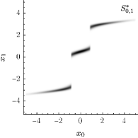
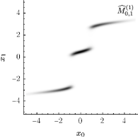
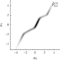
Figure 6: Optimal coupling (left), coupling from the first iteration of the IDBM procedure (center), PM from the first iteration of the IPF procedure (right); generative time.

We discretize $ϒ$ and $Γ$ into $5,000$ equally spaced bins on $[-5,5]$ and solve the corresponding EOT problem using the Sinkhorn algorithm from the POT library (Flamary et al., 2021). For $σ=0.2$, convergence is attained in around $2,000$ iterations with default tolerances. We display the resulting 2D histogram in Figure 6 (left). We additionally plot the 2D kernel density estimates of $\widehat{F}^{(1)}_{0,1}$ (center) and $\widehat{M}^{(1)}_{0,1}$ (right). It can be seen that the first iteration of the IDBM procedure suffices to produce a coupling capturing the overall shape of $S^{*}_{0,1}$.

6.3 Generative Modeling

In this application, we explore the use of the BDBM transport as an alternative to the score-based generative paradigm (Section 2.5) for image generation purposes. The reference SDE is given by 33 with $α=0$ and $Σ=I$, i.e. by a time-scaled $d$-dimensional Brownian motion. We consider the CIFAR-10 dataset, hence $d=28{×}28{×}3$. As baseline modeling choice we consider the “VE SDE” parametrization from Song et al. (2021) for $β_{t}$, and the corresponding smoothed training data distribution $D_{η}$,

$$dX_{t}=\sqrt{β_{t}}dW_{t},\quad t∈[0,1],$$ (43)

$$X_{0}∼D_{η},$$

$$β_{t}≔σ_{\min}^{2}\Big{(}\frac{σ_{\max}}{σ_{\min}}\Big{)}^{2t}2\log\Big{(}\frac{σ_{\max}}{σ_{\min}}\Big{)},$$

$$b_{t}=σ_{\min}^{2}\Big{(}\frac{σ_{\max}}{σ_{\min}}\Big{)}^{2t}-σ_{\min}^{2},$$

where $η=σ_{\min}=10^{-2}$ and $σ_{\max}=50$. We recall that $D_{η}≔\frac{1}{n}∑_{s=1}^{n}𝒩_{d}(x_{s};0,η^{2}I_{d})$. Here $x_{1},…,x_{n}$ are the $50,000$ samples of CIFAR-10’s training dataset $D^{\mathrm{train}}_{\mathrm{CIFAR-10}}$. We select the NCSN++ (smaller) architecture, and training is performed using the official PyTorch implementation of Song et al. (2021). We review the SGM training procedure in Algorithm 3.

Algorithm 3 SGM training

1:$Γ$, $R_{t|0}$, $∇_{y}\log r_{t|0}(y,x)$, $α(θ,x,t)$

2:$α_{\mathrm{SGM}}(x,t)$

3:repeat

4:   $t∼𝒰(0,τ)$

5:   $X_{0}∼Γ$

6:   

7:   $X_{t}∼R_{t|0}(□|X_{0})$

8:   $Y_{t}\textleftarrow∇_{X_{t}}\log r_{t|0}(X_{t}|X_{0})$

9:   $ℒ\textleftarrow\big{\lVert}Y_{t}-α(θ,X_{t},t)\big{\rVert}^{2}λ_{t}$

10:   $θ\textleftarrow\texttt{sgdstep}(θ,ℒ)$

11:until convergence

Algorithm 4 BDBM training

1:$Γ$, $ϒ$, $R_{t|0,τ}$, $∇_{y}\log r_{t|0}(y,x)$, $α(θ,x,t)$

2:$α_{\mathrm{BDBM}}(x,t)$

3:repeat

4:   $t∼𝒰(0,τ)$

5:   $X_{0}∼Γ$

6:   $X_{τ}∼ϒ$

7:   $X_{t}∼R_{t|0,τ}(□|X_{0},X_{τ})$

8:   $Y_{t}\textleftarrow∇_{X_{t}}\log r_{t|0}(X_{t}|X_{0})$

9:   $ℒ\textleftarrow\big{\lVert}Y_{t}-α(θ,X_{t},t)\big{\rVert}^{2}λ_{t}$

10:   $θ\textleftarrow\texttt{sgdstep}(θ,ℒ)$

11:until convergence

Implementing the BDBM approach requires minimal changes, as delineated in Algorithm 4. PyTorch implementations of SGM and BDBM losses are provided for a reference SDE described by 33 with $Σ=I$ and for the regularizer $λ_{t}=v(0,t)$ in Figures 10 and 11 (Appendix C).

By design, the reference SDE 43 strongly decouples $X_{1}$ from $X_{0}$, in which case the BDBM and SGM approaches yield similar generative models. We set $σ_{{\max}}=1$ and keep $ϒ=𝒩_{d}(0,σ_{{\max}}^{2}I)$ for the generative process’s initial distribution, without making efforts to optimize these hyperparameters. Aside from the modifications to the loss function, no additional changes are introduced to the training code, and training proceeds as for the baseline SGM.

The trained neural network approximators obtained from Algorithm 3 and Algorithm 4 corresponds to the drift adjustment factors appearing in 16 and 26 as conditional expectations. As the remaining terms in 16 and 26 are identical, no code changes are necessary when transitioning from SGM to BDBM at generation time.

To assess the visual quality of generated samples, we employ the Fréchet Inception Distance (FID, Heusel et al. (2017)). FID, which aligns with human-perceived visual quality, is calculated as the 2-Wasserstein Euclidean distance in features space, where image features are derived form the Inception model architecture. CIFAR-10 training occurs over $1,300,000$ SGD steps. After every $50,000$ SGD steps, we compute the FID between the test portion of the CIFAR-10 dataset, $D^{\mathrm{test}}_{\mathrm{CIFAR-10}}$, and the corresponding $5,000$ samples generated from the SGM and BDBM models. Sampling is performed using the Euler scheme 11, $Δt=10^{-3}$. The results are presented in Figure 7, illustrating the competitive performance of the BDBM model for this discretization interval. Furthermore, the BDBM approach exhibits significantly accelerated training.

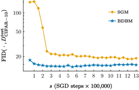
Figure 7: FID between samples generated from the SGM and BDBM models and CIFAR-10 test empirical distribution at $Δt=10^{-3}$; log-scale.

For each of the considered models and their 26 parameter states (checkpoints, at intervals of $50,000$ SGD steps), generating $5,000$ samples from either the SGM or the BDBM model using the Euler scheme with a discretization interval $Δt=10^{-4}$ necessitates approximately one day of computation on the NVIDIA RTX 3090 GPU utilized in this experiment. With the same discretization interval, the predictor-corrector scheme of Song et al. (2021) demands twice the computation time. As such, we have chosen to circumvent the intensive computations required to identify an “optimal” checkpoint through grid-search across parameter states using the predictor-corrector scheme and $Δt=10^{-4}$, as is done in Song et al. (2021). Our analysis is instead confined to the Euler scheme and a single “optimal” checkpoint is selected for both the SGM and BDBM models relying on the findings of Figure 7. For the BDBM model, we opt for the model trained for $250,000$ steps, while for the SGM model we select the model trained for $1,200,000$ steps, which aligns with the checkpoint chosen in Song et al. (2021). Subsequently, we calculate the FID values corresponding to $Δt=1/25,1/100,1/1000$, obtaining $93.7,14.0,12.1$ for the BDBM model and $420.3,18.3,12.0$ for the SGM model, respectively. Corresponding randomly selected samples are shown in Figure 8 and contrasted with the first $16$ CIFAR-10 training samples. Although the visual quality of the SGM and BDBM models is comparable at finer discretization steps, the BDBM model retains superior visual quality as the discretization interval increases.

Figure 8: Samples from the SGM and BDBM models with different discretization intervals, compared to samples from the CIFAR-10 training dataset.

6.4 Dataset Transfer

In this section, we investigate an application where both the initial and the terminal distributions are complex, rendering SGM approaches inapplicable. Following Bortoli et al. (2021), we explore the scenario where the initial distribution $Γ$ is represented by the MNIST dataset ($D_{\mathrm{MNIST}}$), whereas the terminal distribution $ϒ$ is derived from the first five lowercase and the first five uppercase characters, specifically, a,…,e,A,…,E, of the EMNIST dataset ($D_{\mathrm{EMNIST}}$). Consequently, $d=28{×}28$. The reference process law $R$ is associated to $dX_{t}=σdW_{t}$ over the time interval $[0,1]$. Our objective is to approximately solve $(\mathrm{S_{dyn}})$.

We evaluate the performance of the DIPF and IDBM procedures, alternating between solving the IDBM iterations in backward and forward time directions—a requirement for the DIPF procedure. As in Bortoli et al. (2021), we utilize a lightweight configuration of the U-Net neural network architecture as proposed by Dhariwal and Nichol (2021). We employ two neural network models $α(θ,x,t)$, $α(ϕ,x,t)$, which act as approximators to the drifts corresponding to the forward and backward iterations respectively.

Each of these models, $α(θ,x,t)$ and $α(ϕ,x,t)$, is associated with an independent instance of the Adam optimizer due to its adaptive nature, and a model copy ($α(\hat{θ},x,t)$ to $α(θ,x,t)$, $α(\hat{ϕ},x,t)$ to $α(ϕ,x,t)$). The parameters of these copies, $\hat{θ}$ and $\hat{ϕ}$, are updated according to the Exponential Moving Averaging (EMA) scheme. Models $α(\hat{θ},x,t)$ and $α(\hat{ϕ},x,t)$, whose parameters evolve more stably, are used to simulate the required SDE paths using the Euler scheme and a discretization interval of $Δt=1/30$. To increase efficiency, we implement caching of sampled paths. For the DIPF algorithm, entire discretized paths are cached, while for the IDBM algorithm, only the initial and terminal values are cached. Sampling from the reference diffusion bridge corresponding to $R$ at arbitrary time points can be performed quickly and exactly (Section 4).

We utilize the following training methods. For the DIPF procedure, we rely on the drift matching estimator 14. For the IDBM procedure, we employ the regression estimators 27. For the reference process $dX_{t}=σdW_{t}$, both the BDM 34 and BDBM 35 have the same target $(X_{1}-X_{t})/(1-t)$ entering the forward and backward losses in 27. Instead of using time-dependent regularizers as in Section 6.3, we limit the simulation of $t$ to $t∼𝒰(0,1-Δt/2)$, which allows us to recover the Rectified Flow loss with $σ=0$.

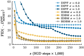
Figure 9: IDBM and DIPF test FID values as function of SGD steps for (left): $D_{\mathrm{EMNIST}}^{\mathrm{test}}\textrightarrow D_{\mathrm{MNIST}}^{\mathrm{test}}$, i.e. backward time; (right): $D_{\mathrm{MNIST}}^{\mathrm{test}}\textrightarrow D_{\mathrm{EMNIST}}^{\mathrm{test}}$, i.e. forward time; linear-scale, truncated at $60$.

Test FID values are calculated by initializing $X_{0}$ from $D_{\mathrm{EMNIST}}^{\mathrm{test}}$ ($D_{\mathrm{MNIST}}^{\mathrm{test}}$) and subsequently sampling the discretized path $X_{t}$ to obtain model samples that are approximately distributed as $D_{\mathrm{MNIST}}^{\mathrm{test}}$ ($D_{\mathrm{EMNIST}}^{\mathrm{test}}$). The specific procedures corresponding to the IDBM and DIPF methods are as follows. For the DIPF procedure, we remove the stochastic component from the terminal Euler discretization step as customary. For the IDBM procedure, we employ the estimator $E_{t}≔𝔼[X_{1}|X_{t}]$, which is directly obtained from $α(\hat{θ},x,t)$ and $α(\hat{ϕ},x,t)$. Evaluating $E_{1-Δt}$ is equivalent to removing the stochastic component from the terminal Euler discretization step, but we find that $E_{1-2Δt}$ empirically performs better.

We consider three different levels of regularization $σ=1.0,0.5,0.2$, and compare the IDBM and DIPF procedures over $60$ iterations, with each iteration comprising $5,000$ SGD steps. Additionally, we assess the simpler application of the BDBM procedure, which is trained for an equivalent amount of $300,000$ SGD steps. Detailed settings of all hyperparameters defining this experiment, along with implementation details, are provided in the accompanying code implementation.

Procedure	IDBM			DIPF			BDBM
Regularization $σ$	$1.0$	$0.5$	$0.2$	$1.0$	$0.5$	$0.2$	$1.0$
FID forward	10.9	6.1	6.8	29.2	23.4	9.8
FID backward	8.2	4.9	5.2	27.6	22.8	11.7	5.3
$𝕃_{\mathrm{OC}}(u,R^{u},Σ_{R})/d$ forward	4.0	5.2	12.5	65.9	31.2	22.5
$𝕃_{\mathrm{OC}}(u,R^{u},Σ_{R})/d$ backward	3.9	4.8	12.5	62.1	33.6	22.5	4.2

Table 2: Test FID and $𝕃_{\mathrm{OC}}(u,R^{u},Σ_{R})$ values for fully trained IDBM, DIPF and BDBM procedures.

The findings from this experiment are presented in Table 2 and Figure 9. The IDBM procedure consistently displays superior convergence properties and lower test FID values compared to the DIPF procedure. For both $σ=0.5$ and $σ=0.2$, the DIPF procedure fails to make significant progress, with model samples almost identical to the input samples. Indeed, a FID value around $30$ corresponds to $\mathrm{FID}(D_{\mathrm{MNIST}}^{\mathrm{test}},D_{\mathrm{EMNIST}}^{\mathrm{test}})$. Visualizations of trajectories of sampled paths $X_{t}$, and of estimators $E_{t}$ for the IDBM and BDBM approaches, are included in Appendix D.

The results from the IDBM procedure also illustrates a dependency on the regularization level $σ$, with performance deteriorating for the lowest regularization level $σ=0.2$. We were unable to achieve satisfactory results for the case $σ=0$, which corresponds to the Rectified Flow method. In this instance a valid transport is not achieved as well, with model samples strongly resembling the input samples. We hypothesize that while the RF method offers the advantageous feature of progressively straightening the inferred paths, the ensuing inference problem may present considerable difficulty. Indeed, the neural network model has to predict the terminal sample exactly at $t=0$ based on the initial sample, which commences to be the case at low levels of $σ$ (see $E_{t}$ in Appendix D).

The optimal SDE solving $(\mathrm{S_{dyn}})$ accomplishes a valid coupling while minimizing the drift norm functional $𝕃_{\mathrm{OC}}(u,R^{u},Σ_{R})$, as outlined in Section 3.2. Lower FID values serve as indicators of the accuracy of the inferred coupling. As demonstrated by the results presented in Table 2, the IDBM procedure not only infers an accurate coupling but also effectively minimizes $𝕃_{\mathrm{OC}}(u,R^{u},Σ_{R})$. Estimations of the test values for $𝕃_{\mathrm{OC}}(u,R^{u},Σ_{R})$ are computed through Monte Carlo sampling of the drift norm functional 20. In this process, the relevant neural network approximator is substituted for $μ(x,t)$. Finally, the simpler BDBM procedure yields FID and $𝕃_{\mathrm{OC}}(u,R^{u},Σ_{R})$ values that are comparable to those produced by the more complex IDBM procedure. This suggests that the BDBM crude approximation to $(\mathrm{S_{dyn}})$ might be acceptable within this context.

7 Discussion

This paper introduces a novel iterative algorithm, the IDBM procedure, aimed at solving the dynamic Schrödinger bridge problem $(\mathrm{S_{dyn}})$, and performs a preliminary theoretical analysis of its convergence properties. The theoretical findings are complemented by various numerical simulations and analytical results, demonstrating the competitive performance of the IDBM procedure in comparison to the IPF procedure.

As in Pavon et al. (2018); Bortoli et al. (2021); Vargas et al. (2021), we assume that samples from the target initial and terminal distributions are either readily available, belonging to some dataset of interest, or can be generated without further approximations. The IDBM procedure is particularly suitable in scenarios where the reference diffusion admits simple analytical transition densities. These considerations suggest that the IDBM procedure is ideally suited for current generative applications. Since the IDBM procedure produces a valid coupling at each iteration, we utilize the first IDBM iteration, i.e. the (backward) DBM transport, as an alternative to the approach of Song et al. (2021). This alternative achieves accelerated training and superior sample quality at larger discretization intervals. An additional advantage of this proposal is the simplicity of its implementation, which differs from the approach of Song et al. (2021) only in the training loss definition. The time-reversal sampling-based implementations of Bortoli et al. (2021); Vargas et al. (2021) suffer from the simulation-inference mismatch demonstrated in the present work, and might be difficult to scale to demanding generative applications due to the ensuing lower efficiency and higher computational cost.

The outcomes of our study give rise to additional avenues for future research. From a theoretical perspective, our initial analysis falls short of establishing the convergence in KL divergence of the IDBM procedure’s iterates to the solution to $(\mathrm{S_{dyn}})$. The numerical and analytical results of Section 6.1 support that, under suitable conditions, this stronger form of convergence is achieved. Non-asymptotic results would be particularly valuable, as they could elucidate the conditions under which either the IPF or IDBM methods are more favorable. Moreover, it would be desirable to introduce more easily verifiable conditions guaranteeing convergence of the IDBM procedure. Finally, when $d>1$, neither the IPF nor the IDBM procedures are robust to vanishing randomness in the reference diffusion $R$. Consequently, the design of an iterative procedure solving $(\mathrm{S_{dyn}})$, while being robust to a vanishing regularization level, remains an open problem.

On the empirical side, computational constraints limited the scope of our simulation study comparing the DBM transport to the time-reversal approach of Song et al. (2021). Specifically, no hyperparameter optimization was performed, neither for DBM-specific parameters, nor for the employed neural network architecture, while Figure 7 suggests that the tested configuration might suffer from overfitting later in training. This is conceivable, as the DBM transport approximates the solution to $(\mathrm{S_{dyn}})$, which is associated to an SDE that has a “simpler” optimal drift (Dai Pra, 1991). Since the exact solution to the DBM transport, and of the competing approaches, perfectly recovers the training data distribution, a less powerful architecture might be required for superior generalization properties. Overfitting to the CIFAR-10 dataset is not a novel concern (Nichol and Dhariwal, 2021), and it is typically addressed through hyperparameter search.

At one extreme, when the reference process’s dynamics imply a terminal value almost independent of the initial value, the DBM results in a generative model akin to that of Song et al. (2021), while rectifying the terminal distribution mismatch inherent in all time-reversal approaches (Bortoli et al., 2021). More generally, the DBM transport enlarges the space of feasible (exact) transports. Consequently, it is plausible that improvements in current state-of-the-art solutions can be attained by empirically exploring this enlarged space, optimizing for a given metric of interest, such as FID. In particular, high-resolution images pose challenges for time-reversal approaches and necessitate an increase in the reference process randomness, thus increasing the implicit integration time (Hoogeboom et al., 2023). The DBM transport, which precisely matches the initial and terminal marginal distributions, does not face this issue. Lastly, computational constraints precluded an evaluation of the application of further iterations of the IDBM procedure in generative modeling applications, which would trade off increased training time with a more efficient generation process.

The approaches of Bortoli et al. (2021); Vargas et al. (2021) are directly applicable to a broad spectrum of reference SDEs. Conversely, the IDBM procedure detailed in this work necessitates an analytically solvable reference SDE. However, we remark that the IDBM methodology can potentially be extended to accommodate complex reference dynamics. A promising approach involves harnessing the findings of De Bortoli et al. (2021) to construct neural network approximators for $∇_{x}\log(r_{τ|t}(y|x))$ and $∇_{y}\log(r_{t|0}(y|x))$. These approximators allow both the sampling of the reference diffusion bridge via a discretization of 17, and the calculation of the targets in the estimators 27. An alternative strategy employs the Exact Algorithm (EA) proposed by Beskos and Roberts (2005); Beskos et al. (2008) to sample exactly from the reference diffusion bridge 17. The unavailability of $∇_{x}\log(r_{τ|t}(y|x))$ and $∇_{y}\log(r_{t|0}(y|x))$ can be circumvented by performing drift inference as outlined in Section 2.4, rather than relying on 27. We refer to the discussion following LABEL:{eq:dbm_drift_inference} for more details. However, we must underscore that the application of the EA is restricted to reference SDEs with a “reducible” diffusion coefficient (Aït-Sahalia, 2008), and to low-dimensional spaces due to scalability concerns (Peluchetti and Roberts, 2012). We refer to Beskos et al. (2008) for the additional requirements on the drift coefficient of the reference SDE. The empirical evaluation of these extensions is left to future research.

Appendix A Proofs

Proof of Theorem 1

The following assumptions are sufficient for the application of Theorem 1. We assume that 23 and each member of 21 admit a unique solution, with strictly positive marginal densities over $ℝ^{d}$. We assume that each marginal density is the unique solution to the corresponding Fokker-Plank PDE, and that the exchanges of limits denoted with $(\star\star)$ hold. When Theorem 1 is applied to match $Π=CR_{\textbullet|0,τ}$ in Section 3.4, these conditions are satisfied if $R$ is given by 33 and the marginal distributions of $C$ are given by mixtures of Gaussian distributions, which covers the setting of generative modelling applications.

See 1

Proof  In this proof we make use of the following notation: for $f(x,t):ℝ^{d}×[0,τ]\textrightarrow ℝ$, ${(f(x,t))}_{t}≔\frac{d}{dt}f(x,t)$, for $f(x,t):ℝ^{d}×[0,τ]\textrightarrow ℝ^{d}$, ${(f(x,t))}_{x}≔\sum_{i=1}^{d}\frac{d}{dx_{i}}[f]_{i}(x,t)$, for $f(x,t):ℝ^{d}×[0,τ]\textrightarrow ℝ^{d}×ℝ^{d}$, ${(f(x,t))}_{xx}≔\sum_{i,j=1}^{d}\frac{d^{2}}{dx_{i}dx_{j}}[f]_{i,j}(x,t)$. Let $Σ^{λ}(x,t)≔σ^{λ}(x,t)σ^{λ}(x,t)ᵀ$. Then, for $0<t≤τ$,

$${(π_{t}(x))}_{t}={\left(∫_{Λ}p_{t}^{λ}(x)Ψ(dλ)\right)}_{t}$$

$$\quad=∫_{Λ}{\left(p_{t}^{λ}(x)\right)}_{t}Ψ(dλ) \star\star$$ ()

$$\quad=∫_{Λ}{\left(\mu^{λ}(x,t)p_{t}^{λ}(x)\right)}_{x}+\frac{1}{2}{\left(Σ^{λ}(x,t)p_{t}^{λ}(x)\right)}_{xx}Ψ(dλ)$$

$$\quad=∫_{Λ}{\left(\frac{\mu^{λ}(x,t)p_{t}^{λ}(x)}{π_{t}(x)}π_{t}(x)\right)}_{x}+\frac{1}{2}{\left(\frac{Σ^{λ}(x,t)p_{t}^{λ}(x)}{π_{t}(x)}π_{t}(x)\right)}_{xx}Ψ(dλ)$$

$$\quad={\left(∫_{Λ}\frac{\mu^{λ}(x,t)p_{t}^{λ}(x)}{π_{t}(x)}Ψ(dλ)π_{t}(x)\right)}_{x}+\frac{1}{2}{\left(∫_{Λ}\frac{Σ^{λ}(x,t)p_{t}^{λ}(x)}{π_{t}(x)}Ψ(dλ)π_{t}(x)\right)}_{xx}. \star\star$$ ()

The lines denoted with $(\star\star)$ consist of exchange of limits, the third line results from the application of the Fokker-Plank PDEs for $\{P^{λ}\}_{λ∈Λ}$. The Fokker-Plank PDE for 23 is

$${(p_{t}(x))}_{t}={\left(∫_{Λ}\frac{\mu^{λ}(x,t)p_{t}^{λ}(x)}{π_{t}(x)}Ψ(dλ)p_{t}(x)\right)}_{x}+\frac{1}{2}{\left(∫_{Λ}\frac{Σ^{λ}(x,t)p_{t}^{λ}(x)}{π_{t}(x)}Ψ(dλ)p_{t}(x)\right)}_{xx}.$$

As $P_{0}=Π_{0}$ and $p$ and $π$ satisfy the same Fokker-Plank PDE, it follows that $P$ and $Π$ share the same marginal distribution.  

Proof of Theorem 2

See 2

Proof  Let $P∈𝒫_{𝒞}$ be the law of the diffusion solving

$$dX_{t}=μ(X_{t},t)dt+σ_{R}(X_{t},t)dW_{t},\quad t∈[0,τ],$$

$$X_{0}∼P_{0}.$$

Let $C∈𝒫_{2}(Γ,ϒ)$. Within this proof, we use the following abbreviations: $Π(C)≔Π(C,R_{\textbullet|0,τ})$, $M(C)≔M(Π(C,R_{\textbullet|0,τ}))$, $S^{*}≔S^{*}(Γ,ϒ,R,𝒫_{𝒞})$. Assume that $D_{KL}(Π(C)\mathbin{\textbardbl}P)<∞$ and that the conditions required for the application of the Cameron-Martin-Girsanov theorem to obtain $dM(C)/dP$ are satisfied. As $M(C)≪P$ as well, following Csiszar (1975), it holds that

$$D_{KL}(Π(C)\mathbin{\textbardbl}P)-D_{KL}(Π(C)\mathbin{\textbardbl}M(C)) =𝔼_{Π(C)}\Big{[}\log\frac{dΠ(C)}{dP}\Big{]}-𝔼_{Π(C)}\Big{[}\log\frac{dΠ(C)}{dM(C)}\Big{]}$$

$$=𝔼_{Π(C)}\Big{[}\log\frac{dM(C)}{dP}\Big{]},$$

and we want to show that

$$𝔼_{Π(C)}\Big{[}\log\frac{dM(C)}{dP}\Big{]}=𝔼_{M(C)}\Big{[}\log\frac{dM(C)}{dP}\Big{]}.$$

As $Π_{0}(C)=M_{0}(C)=Γ$ it suffices to show that

$$𝔼_{Π(C)}\Big{[}\log\frac{dM_{\textbullet|0}(C)}{dP_{\textbullet|0}}\Big{]}=𝔼_{M(C)}\Big{[}\log\frac{dM_{\textbullet|0}(C)}{dP_{\textbullet|0}}\Big{]},$$

where

$$\log\frac{dM_{\textbullet|0}(C)}{dP_{\textbullet|0}}(x)=∫_{0}^{τ}[(μ_{M}-μ)ᵀΣ_{R}^{-1}](x_{t},t)dx_{t}-\frac{1}{2}∫_{0}^{τ}[(μ_{M}-μ)ᵀΣ_{R}^{-1}(μ_{M}+μ)](x_{t},t)dt$$

is given by 12. As $Π(δ_{x_{0}}{⊗}ϒ,R_{\textbullet|0,τ})=Π_{\textbullet|0}(C,R_{\textbullet|0,τ})$, from 25,

$$𝔼_{Π(C)}\Big{[}∫_{0}^{τ}[(μ_{M}-μ)ᵀΣ_{R}^{-1}](X_{t},t)dX_{t}\Big{]}$$

$$\quad=𝔼_{Π(C)}\Big{[}∫_{0}^{τ}[(μ_{M}-μ)ᵀΣ_{R}^{-1}](X_{t},t)\big{(}μ_{R}(X_{t},t)+Σ_{R}(X_{t},t)𝔼_{Π(C)}[∇_{X_{t}}\log r_{τ|t}(X_{τ}|X_{t})|X_{t},X_{0}]\big{)}dt\Big{]}$$

$$\quad=𝔼_{Π(C)}\Big{[}∫_{0}^{τ}[(μ_{M}-μ)ᵀΣ_{R}^{-1}](X_{t},t)\big{(}μ_{R}(X_{t},t)+Σ_{R}(X_{t},t)𝔼_{Π(C)}[∇_{X_{t}}\log r_{τ|t}(X_{τ}|X_{t})|X_{t}]\big{)}dt\Big{]},$$

by the tower property of conditional expectations. On the other hand, from 24,

$$𝔼_{M(C)}\Big{[}∫_{0}^{τ}[(μ_{M}-μ)ᵀΣ_{R}^{-1}](X_{t},t)dX_{t}\Big{]}$$

$$\quad=𝔼_{M(C)}\Big{[}∫_{0}^{τ}[(μ_{M}-μ)ᵀΣ_{R}^{-1}](X_{t},t)\big{(}μ_{R}(X_{t},t)+Σ_{R}(X_{t},t)𝔼_{Π(C)}[∇_{X_{t}}\log r_{τ|t}(X_{τ}|X_{t})|X_{t}]\big{)}dt\Big{]}$$

$$\quad=𝔼_{Π(C)}\Big{[}∫_{0}^{τ}[(μ_{M}-μ)ᵀΣ_{R}^{-1}](X_{t},t)\big{(}μ_{R}(X_{t},t)+Σ_{R}(X_{t},t)𝔼_{Π(C)}[∇_{X_{t}}\log r_{τ|t}(X_{τ}|X_{t})|X_{t}]\big{)}dt\Big{]},$$

as $M_{t}(C)=Π_{t}(C)$ for all $t∈[0,τ]$. In the same way, equality in expectations of $-\frac{1}{2}∫_{0}^{τ}[(μ_{M}-μ)ᵀΣ_{R}^{-1}(μ_{M}+μ)](X_{t},t)dt$ is established. We thus obtain a version of the Pythagorean law for (reverse) KL-projections (Csiszar, 1975; Nielsen, 2018),

$$D_{KL}(Π(C)\mathbin{\textbardbl}P)=D_{KL}(Π(C)\mathbin{\textbardbl}M(C))+D_{KL}(M(C)\mathbin{\textbardbl}P).$$

See also Liu et al. (2023b) for another derivation of this result. When $P=S^{*}$ ($S^{*}$ is law of the diffusion solving LABEL:eq:schrodinger_sde), under the same assumptions,

$$D_{KL}(Π(C)\mathbin{\textbardbl}S^{*})≥D_{KL}(M(C)\mathbin{\textbardbl}S^{*}),$$ (44)

with equality if and only if $Π(C)=M(C)$.

If $Π(C)=S^{*}$, then $M(C)=S^{*}$ as $Π(C)=CR_{\textbullet|0,τ}$ is equal in law to the diffusion process solving LABEL:eq:schrodinger_sde and Theorem 1 applied to a (single) diffusion results in that same diffusion. On the other hand, if $Π(C)≠S^{*}$, then $Π(C)$ is not a diffusion (it is an Ito process in the sense of Øksendal (2003)), see Section 3.2, and $M(C)≠Π(C)$ (Øksendal, 2003, Theorem 8.4.3). That is $Π(C)=M(C)$ if and only if $Π(C)=M(C)=S^{*}$.

For $i≥0$,

$$D_{KL}(Π^{(i)}\mathbin{\textbardbl}S^{*}) =D_{KL}(Π^{(i)}_{0,τ}\mathbin{\textbardbl}S^{*}_{0,τ})+𝔼_{Π^{(i)}_{0,τ}}[D_{KL}(Π^{(i)}_{\textbullet|0,τ}\mathbin{\textbardbl}S^{*}_{\textbullet|0,τ})]$$

$$=D_{KL}(Π^{(i)}_{0,τ}\mathbin{\textbardbl}S^{*}_{0,τ}),$$

as $Π^{(i)}_{\textbullet|0,τ}=S^{*}_{\textbullet|0,τ}=R_{\textbullet|0,τ}$, and

$$D_{KL}(M^{(i)}\mathbin{\textbardbl}S^{*}) =D_{KL}(M^{(i)}_{0,τ}\mathbin{\textbardbl}S^{*}_{0,τ})+𝔼_{M^{(i)}_{0,τ}}[D_{KL}(M^{(i)}_{\textbullet|0,τ}\mathbin{\textbardbl}S^{*}_{\textbullet|0,τ})]$$

$$≥D_{KL}(Π^{(i+1)}_{0,τ}\mathbin{\textbardbl}S^{*}_{0,τ}),$$

as $M^{(i)}_{0,τ}=Π^{(i+1)}_{0,τ}$. Thus,

$$D_{KL}(M^{(i)}\mathbin{\textbardbl}S^{*})≥D_{KL}(Π^{(i+1)}\mathbin{\textbardbl}S^{*}).$$ (45)

It is assumed that $D_{KL}(Π^{(0)}\mathbin{\textbardbl}S^{*})=D_{KL}(C^{(0)}\mathbin{\textbardbl}S^{*}_{0,τ})<∞$, and that the Cameron-Martin-Girsanov theorem applies to each $M^{(i)}$ yielding $dM^{(i)}/dS^{*}$. Therefore, we can iteratively apply 44 and 45 obtaining $D_{KL}(Π^{(i)}\mathbin{\textbardbl}S^{*})≥D_{KL}(M^{(i)}\mathbin{\textbardbl}S^{*})≥D_{KL}(Π^{(i+1)}\mathbin{\textbardbl}S^{*})$ for $i≥0$. Being non-increasing and bounded below, the sequence $D_{KL}(Π^{(i)}\mathbin{\textbardbl}S^{*}),D_{KL}(M^{(i)}\mathbin{\textbardbl}S^{*}),D_{KL}(Π^{(i+1)}\mathbin{\textbardbl}S^{*})$ converges, and $\lim_{i\textrightarrow∞}(D_{KL}(Π^{(i)}\mathbin{\textbardbl}S^{*})-D_{KL}(M^{(i)}\mathbin{\textbardbl}S^{*}))=\lim_{i\textrightarrow∞}D_{KL}(Π^{(i)}\mathbin{\textbardbl}M^{{i}})=0$.

The sequences $\{Π^{(i)}\}_{i≥0}$, $\{M^{(i)}\}_{i≥0}$ are tight. We consider $\{Π^{(i)}\}_{i≥0}$, the case of $\{M^{(i)}\}_{i≥0}$ being identical. By the conditional Jensen inequality, for any measurable set $K$,

$$D_{KL}(Π^{(i)}\mathbin{\textbardbl}S^{*}) =𝔼_{Π^{(i)}}\Big{[}-\log\frac{dS^{*}}{dΠ^{(i)}}\mathrel{\Big{|}}K^{c}\Big{]}Π^{(i)}[K^{c}]+𝔼_{Π^{(i)}}\Big{[}-\log\frac{dS^{*}}{dΠ^{(i)}}\mathrel{\Big{|}}K\Big{]}Π^{(i)}[K]$$

$$≥-\log(S^{*}[K^{c}]/Π^{(i)}[K^{c}])Π^{(i)}[K^{c}]+-\log(S^{*}[K]/Π^{(i)}[K])Π^{(i)}[K].$$

For $ε>0$, choose $K$ compact such $S^{*}[K^{c}]<ε$, $S^{*}[K]≥1-ε$ by the tightness of $S^{*}$ (as it is defined on a Polish space, see Léonard (2014a)). Assume that $Π^{(i)}$ is not tight. That is, there is $γ>0$ such that for each compact $K$ there is $i≥0$ with $Π^{(i)}[K^{c}]≥γ,Π^{(i)}[K]<1-γ$. Hence, for each $ε>0$, there is $i≥0$ such that

$$-\log(S^{*}[K^{c}]/Π^{(i)}[K^{c}])Π^{(i)}[K^{c}]≥-\log(ε/γ)γ,$$

which can be made arbitrarily large by a suitable small $ε>0$. On the other hand, $-\log(S^{*}[K]/x)x$ is bounded below for $x∈[0,1]$, so $-\log(S^{*}[K]/Π^{(i)}[K])Π^{(i)}[K]$ is bounded below. But we know that for $i$ large enough $D_{KL}(Π^{(i)}\mathbin{\textbardbl}S^{*})$ is bounded above, hence $Π^{(i)}$ must be tight.

Therefore, $\{Π^{(i)}\}_{i≥0}$ and $\{M^{(i)}\}_{i≥0}$ are relatively compact. Each subsequence of $\{Π^{(i)}\}_{i≥0}$ has a further subsequence $\{Π^{(l)}\}_{l≥1}$ which converges in law: $Π^{(l)}\overset{ℒ}{⟶}Π^{(∞)}$ as $l\textrightarrow∞$ for some $Π^{(∞)}∈𝒫_{𝒞}(Γ,ϒ)$. Each subsequence of $\{M^{(i)}\}_{i≥0}$ has a further subsequence $\{M^{(l)}\}_{l≥1}$ which converges in law: $M^{(l)}\overset{ℒ}{⟶}M^{(∞)}$ for some $M^{(∞)}∈𝒫_{𝒞}(Γ,ϒ)$. By the lower semi-continuity of the KL divergence with respect to the topology of weak convergence (van Erven and Harremos, 2014, Theorem 19), $0=\liminf_{l\textrightarrow∞}D_{KL}(Π^{(l)}\mathbin{\textbardbl}M^{{i}})≥D_{KL}(Π^{(∞)}\mathbin{\textbardbl}M^{{∞}})$ and therefore $Π^{(∞)}=M^{(∞)}$. Denote this common PM with $S^{(∞)}$.

Due to the convergence in law of $Π^{(l)}$, and the form of its disintegration, $S^{(∞)}$ is of the form $S^{(∞)}_{0,τ}R_{\textbullet|0,τ}$ for some $S^{(∞)}_{0,τ}∈𝒫_{2}(Γ,ϒ)$. If $S^{(∞)}$ is also diffusion, it follows that $S^{(∞)}_{0,τ}=S^{(*)}_{0,τ}$ (Section 3.2) and thus $S^{(∞)}=S^{*}$. It remains to show that $S^{(∞)}$ is a diffusion when $σ_{R}(x,t)=I$. Again by the lower semi-continuity of the KL divergence, we have that $D_{KL}(S^{(∞)}\mathbin{\textbardbl}S^{*})<∞$ and thus $S^{(∞)}≪S^{*}$. But $S^{*}≪R$ and $R≪R^{\circ}$ by assumption where $R^{\circ}$ is the $d$-dimensional Brownian measure on $[0,τ]$. Then, by Liptser and Shiriaev (1977, Theorem 7.11 and following Note 1), $S^{(∞)}$ is a diffusion.

As convergence in law to $S^{*}$ has been established for arbitrary convergent subsequences, $\{Π^{(i)}\}\overset{ℒ}{⟶}S^{(∞)}$ and $\{M^{(i)}\}\overset{ℒ}{⟶}S^{(∞)}$ by Billingsley (1999, Theorem 2.6).  

Appendix B Additional SDE Class Formulae

The linearity of 30 and 31 stands behind the form of the conditional expectations entering the drift coefficients that follow. The generative time reversal process 16 is given by

$$d\overline{X}_{t}=\Big{[}αβ_{𝔯}\overline{X}_{t}+β_{𝔯}\frac{𝔼_{R}[\overline{X}_{τ}|\overline{X}_{t}]a(0,b_{𝔯})-\overline{X}_{t}}{v(0,b_{𝔯})}\Big{]}dt+\sqrt{β_{𝔯}}Γ^{1/2}dW_{t},\quad t∈[0,τ],$$

$$\overline{X}_{0}∼R_{τ}≈ϒ,$$

the DBM transport 24 is given by

$$dX_{t}=\Big{[}-αβ_{t}X_{t}+β_{t}\frac{𝔼_{Π}[X_{τ}|X_{t}]a(b_{t},b_{τ})-X_{t}a(b_{t},b_{τ})^{2}}{v(b_{t},b_{τ})}\Big{]}dt+\sqrt{β_{t}}Γ^{1/2}dW_{t},\quad t∈[0,τ],$$

$$X_{0}∼Γ,$$

while the BDBM transport 26 is given by

$$d\overline{X}_{t}=\Big{[}αβ_{t}\overline{X}_{t}+β_{𝔯}\frac{𝔼_{Π}[\overline{X}_{τ}|\overline{X}_{t}]a(0,b_{𝔯})-\overline{X}_{t}}{v(0,b_{𝔯})}\Big{]}dt+\sqrt{β_{𝔯}}Γ^{1/2}dW_{t},\quad t∈[0,τ],$$

$$\overline{X}_{0}∼ϒ.$$

For $α=0$, the DBM and BDBM transports are symmetric in the following sense: the BDM transport based on $C∈𝒫_{2}(Γ,ϒ)$ and $β_{t}$ is equivalent in law to the BDBM transport based on $\overline{C}∈𝒫_{2}(ϒ,Γ)$ and $\overline{β}_{t}≔β_{𝔯}$.

Appendix C Generative Modeling Code

⬇

# requires:

# b_t(t): $b_t(t)$

# a_s_t(s, t): $a(s, t)$ from (29)

# v_s_t(s, t): $v(s, t)$ from (29)

# inputs:

# x_0: [B,C,H,W]

# model: ([B,C,H,W], [B]) -> [B,C,H,W]

# outputs:

# losses: [B]

def sgm_loss(x_0, model, T=1.0):

t = torch.rand(x_0.shape[0], device=x_0.device) * T # [B]

scaled_t = b_t(t) # [B]

z = torch.randn_like(x_0) # [B,C,H,W]

a_0_t, v_0_t = a_s_t(0.0, scaled_t), v_s_t(0.0, scaled_t) # [B]

s_0_t = torch.sqrt(v_0_t) # [B]

x_t = a_0_t[:, None, None, None] * x_0 + s_0_t[:, None, None, None] * z # [B,C,H,W]

score_t = (x_0 * a_0_t[:, None, None, None] - x_t) / v_0_t[:, None, None, None] # [B,C,H,W]

losses = (model(x_t, scaled_t) - score_t)**2 * v_0_t[:, None, None, None] # [B,C,H,W]

losses = torch.sum(losses.view(losses.shape[0], -1), dim=1) # [B]

return losses

Figure 10: SGM loss sampling; x_0 is a batch of B images, each of which has C channels, height H and width W.

⬇

# requires:

# b_t(t): $b_t(t)$

# a_s_t(s, t): $a(s, t)$ from (29)

# v_s_t(s, t): $v(s, t)$ from (29)

# al_s_t_u(s, t, u): $\hat{a}(s,t,u)$ from (32)

# ar_s_t_u(s, t, u): $\check{a}(s,t,u)$ from (32)

# vb_s_t_u(s, t, u): $\tilde{v}(s,t,u)$ from (32)

# inputs:

# x_0: [B,C,H,W]

# model: ([B,C,H,W], [B]) -> [B,C,H,W]

# outputs:

# losses: [B]

def bdbm_loss(x_0, model, T=1.0, sigma_T=1.0):

t = torch.rand(x_0.shape[0], device=x_0.device) * T # [B]

scaled_t, scaled_T = b_t(t), b_t(T) # [B]

z = torch.randn_like(x_0) # [B,C,H,W]

a_0_t, v_0_t = a_s_t(0.0, scaled_t), v_s_t(0.0, scaled_t) # [B]

x_T = torch.randn_like(x_0) * sigma_T # [B,C,H,W]

al_0_t_T, ar_0_t_T, = al_s_t_u(0.0, t, scaled_T), ar_s_t_u(0.0, t, scaled_T) # [B]

vb_0_t_T = vb_s_t_u(0.0, t, scaled_T) # [B]

sb_0_t_T = torch.sqrt(vb_0_t_T) # [B]

x_t = (

+ al_0_t_T[:, None, None, None] * x_0

+ ar_0_t_T[:, None, None, None] * x_T

+ sb_0_t_T[:, None, None, None] * z

) # [B,C,H,W]

score_t = (x_0 * a_0_t[:, None, None, None] - x_t) / v_0_t[:, None, None, None] # [B,C,H,W]

losses = (model(x_t, scaled_t) - score_t)**2 * v_0_t[:, None, None, None] # [B,C,H,W]

losses = torch.sum(losses.view(losses.shape[0], -1), dim=1) # [B]

return losses

Figure 11: BDBM loss sampling; x_0 is a batch of B images, each of which has C channels, height H and width W.

Appendix D Additional Experimental Results

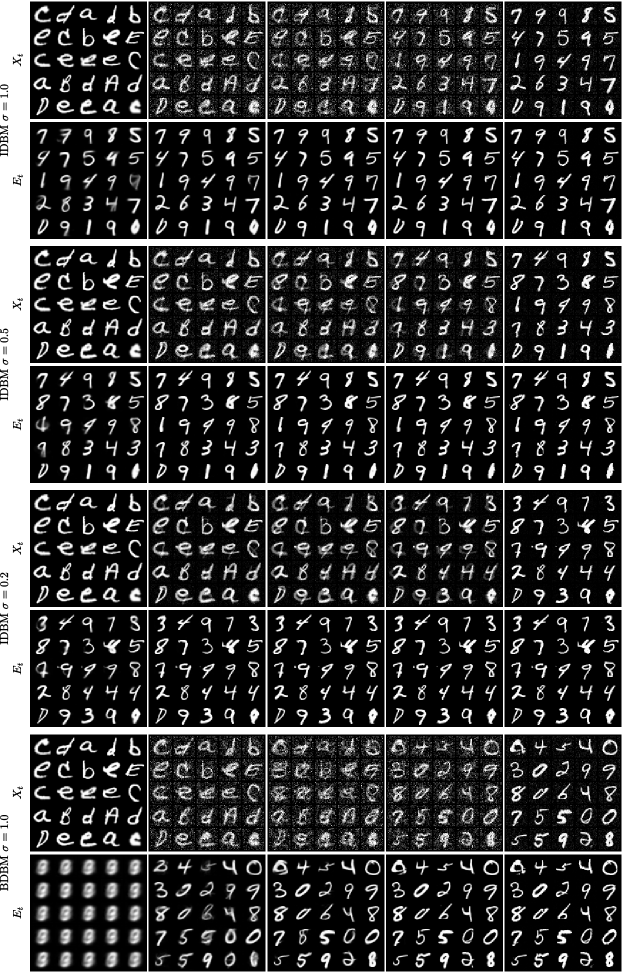
Figure 12: Random paths $X_{t}$ and corresponding terminal value estimators $E_{t}$ for fully trained BDBM and IDBM procedures corresponding to different regularization levels; backward time direction; $t$ uniformly spaced on $[0,1]$ for $X_{t}$, $[0,1-Δt]$ for $E_{t}$; $X_{0}∼D_{\mathrm{EMNIST}}^{\mathrm{test}}$ is fixed.

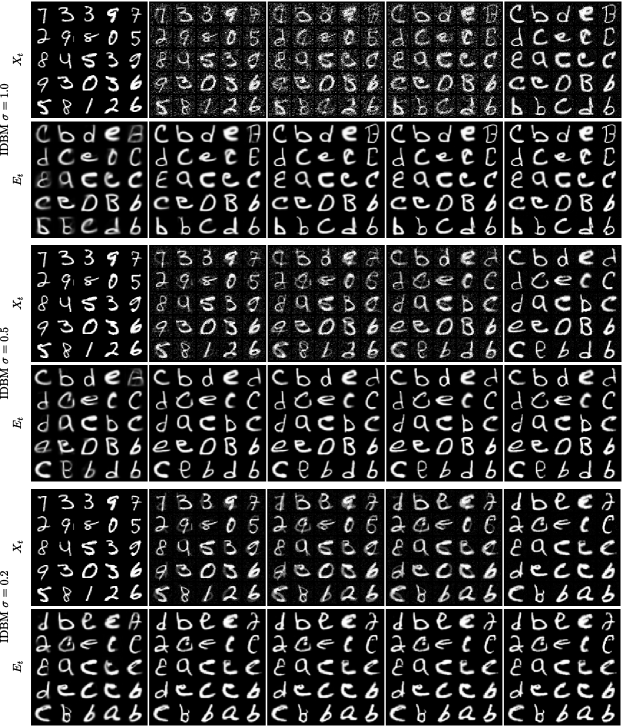
Figure 13: Random paths $X_{t}$ and corresponding terminal value estimators $E_{t}$ for fully trained IDBM procedures corresponding to different regularization levels; forward time direction; $t$ uniformly spaced on $[0,1]$ for $X_{t}$, $[0,1-Δt]$ for $E_{t}$; $X_{0}∼D_{\mathrm{MNIST}}^{\mathrm{test}}$ is fixed.

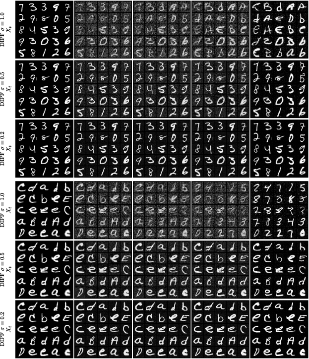
Figure 14: Random paths $X_{t}$ for fully trained DIPF procedures corresponding to different regularization levels; forward (first three rows) and backward (last three rows) time directions; $t$ uniformly spaced on $[0,1]$; $X_{0}∼D_{\mathrm{MNIST}}^{\mathrm{test}}$ (forward time) and $X_{0}∼D_{\mathrm{EMNIST}}^{\mathrm{test}}$ (backward time) are fixed.

Appendix E Notation

Notation	Description
$[0,τ]$	Time interval
$d$	Dimension of state space
$P$, $Q$, $…$	Probability measure (PM)
$𝒫_{𝒞}$	PMs over $𝒞([0,τ],ℝ^{d})$
$𝒫_{n}$	PMs over $ℝ^{d×n}$
$𝒫_{𝒞}(Γ,ϒ)$	PMs with initial-terminal distributions $Γ,ϒ$; $𝒫_{𝒞}(Γ,ϒ)⊆𝒫_{𝒞}$
$𝒫_{2}(Γ,ϒ)$	PMs with marginal distributions $Γ,ϒ$; $𝒫_{2}(Γ,ϒ)⊆𝒫_{2}$
$𝒰(0,τ)$	Uniform distribution on $(0,τ)$
$𝒩_{d}(μ,Σ)$	$d$-variate normal distribution with mean $μ$ and covariance $Σ$
$dP/dQ$	Density of PM $P$ with respect to PM $Q$
$p$	Lebesgue density of PM $P$
$P_{t_{1},…,t_{n}}$	Marginalization of $P∈𝒫_{𝒞}$ at $t_{1},…,t_{n}$
$P_{\textbullet|t_{1},…,t_{n}}$	Conditioning of $P∈𝒫_{𝒞}$ given values at $t_{1},…,t_{n}$
$P=P_{t_{1},…,t_{n}}P_{\textbullet|t_{1},…,t_{n}}$	Marginal-conditional decomposition of $P∈𝒫_{𝒞}$
$Q=ΨP_{\textbullet|t_{1},…,t_{n}}$	Mixing of $P∈𝒫_{𝒞}$ via $Ψ∈𝒫_{n}$ at times $t_{1},…,t_{n}$; $Q∈𝒫_{𝒞}$
$D_{KL}(S\mathbin{\textbardbl}R)$	Kullback-Leibler divergence from PM $S$ to PM $R$
$I$	Identity matrix
$Aᵀ$	Transposition of a square matrix $A$
$\textbardbl V\textbardbl$	Euclidean norm of a vector $V$
$\overline{X}$	Time reversal of stochastic process $X$
$\overline{P}$	Time reversal of PM $P$; $P∈𝒫_{𝒞}$
$𝔯$	Reverse timescale; $𝔯≔τ-t$
$W$	$d$-dimensional standard Brownian motion
$Γ$, $ϒ$	Target PMs; $Γ,ϒ∈𝒫_{1}$
$R$	Reference PM; $R∈𝒫_{𝒞}$
$μ_{R}(x,t)$, $σ_{R}(x,t)$	Reference SDE drift and diffusion coefficients
$Σ_{R}(x,t)$	Reference SDE covariance coefficient; $Σ_{R}≔σ_{R}σ_{R}ᵀ$
$S^{*}(Γ,ϒ,R,𝒫_{𝒞})$	Solution $(\mathrm{S_{dyn}})$ (dynamic)
$S^{*}(Γ,ϒ,R_{0,τ},𝒫_{2})$	Solution to $(\mathrm{S_{sta}})$ (static) (corresponding to $(\mathrm{S_{dyn}})$)
$S^{*}(Γ,□,Q,𝒫)$	Solution to forward $(\mathrm{H_{dyn}})$ ($𝒫=𝒫_{𝒞}$), $(\mathrm{H_{sta}})$ ($𝒫=𝒫_{2}$); $Q∈𝒫$
$S^{*}(□,ϒ,Q,𝒫)$	Solution to backward $(\mathrm{H_{dyn}})$ ($𝒫=𝒫_{𝒞}$), $(\mathrm{H_{sta}})$ ($𝒫=𝒫_{2}$); $Q∈𝒫$
$F^{(i)}$	$i$-th IPF iteration; $F^{(i)}∈𝒫_{𝒞}∪𝒫_{2}$, $i≥0$
$μ_{F^{(i)}}$	Drift corresponding to $F^{(i)}∈𝒫_{C}$
$Π(C,R_{\textbullet|0,τ})$	Diffusion mixture; $C∈𝒫_{2}(Γ,ϒ)$, $Π∈𝒫_{𝒞}(Γ,ϒ)$
$M(Π(C,R_{\textbullet|0,τ}))$	Forward DBM based on $C$; $C∈𝒫_{2}(Γ,ϒ)$, $M∈𝒫_{𝒞}(Γ,ϒ)$
$\overline{M}(Π(C,R_{\textbullet|0,τ}))$	Backward DBM based on $C$; $C∈𝒫_{2}(Γ,ϒ)$, $\overline{M}∈𝒫_{𝒞}(ϒ,Γ)$
$M^{(i)}$	$i$-th (forward) IDBM iteration; $M^{(i)}∈𝒫_{𝒞}$, $i≥0$
$C^{(i)}$	$i$-th IDBM coupling; $C^{(i)}∈𝒫_{2}(Γ,ϒ)$, $C^{(i)}≔M^{(i)}_{0,τ}$
$Π^{(i)}$	$i$-th IDBM diffusion mixture; $Π^{(i)}∈𝒫_{𝒞}$, $Π^{(i)}≔Π(C^{(i-1)},R_{\textbullet|0,τ})$
$μ_{M^{(i)}}$	Drift corresponding to $M^{(i)}∈𝒫_{𝒞}$

Table 3: Main notation summary.

References

- Anderson (1982) Brian D.O. Anderson. Reverse-Time Diffusion Equation Models. Stochastic Processes and their Applications, 12(3):313–326, May 1982.
- Aït-Sahalia (2008) Yacine Aït-Sahalia. Closed-form likelihood expansions for multivariate diffusions. The Annals of Statistics, 36(2):906–937, 2008. ISSN 0090-5364, 2168-8966.
- Bernton et al. (2019) Espen Bernton, Jeremy Heng, Arnaud Doucet, and Pierre E. Jacob. Schrödinger Bridge Samplers, 2019.
- Beskos and Roberts (2005) Alexandros Beskos and Gareth O. Roberts. Exact simulation of diffusions. The Annals of Applied Probability, 15(4):2422–2444, 2005. ISSN 1050-5164, 2168-8737.
- Beskos et al. (2008) Alexandros Beskos, Omiros Papaspiliopoulos, and Gareth O. Roberts. A Factorisation of Diffusion Measure and Finite Sample Path Constructions. Methodology and Computing in Applied Probability, 10(1):85–104, 2008. ISSN 1573-7713.
- Billingsley (1999) Patrick Billingsley. Convergence of Probability Measures. Wiley Series in Probability and Statistics. Probability and Statistics Section. Wiley, 2nd ed edition, 1999.
- Bortoli et al. (2021) Valentin De Bortoli, James Thornton, Jeremy Heng, and Arnaud Doucet. Diffusion Schrödinger Bridge with Applications to Score-Based Generative Modeling. In Thirty-Fifth Conference on Neural Information Processing Systems, 2021.
- Brigo (2002) Damiano Brigo. The General Mixture-Diffusion SDE and Its Relationship with an Uncertain-Volatility Option Model with Volatility-Asset Decorrelation, December 2002.
- Brooks et al. (2011) Steve Brooks, Andrew Gelman, Galin Jones, and Xiao-Li Meng. Handbook of Markov Chain Monte Carlo. CRC press, 2011.
- Chen et al. (2022) Tianrong Chen, Guan-Horng Liu, and Evangelos Theodorou. Likelihood Training of Schrödinger Bridge using Forward-Backward SDEs Theory. In International Conference on Learning Representations, 2022.
- Csiszar (1975) I. Csiszar. I-Divergence Geometry of Probability Distributions and Minimization Problems. The Annals of Probability, 3(1):146–158, 1975. ISSN 0091-1798.
- Dai Pra (1991) Paolo Dai Pra. A stochastic control approach to reciprocal diffusion processes. Applied Mathematics and Optimization, 23(1):313–329, 1991. ISSN 1432-0606.
- De Bortoli et al. (2021) Valentin De Bortoli, Arnaud Doucet, Jeremy Heng, and James Thornton. Simulating Diffusion Bridges with Score Matching, 2021.
- Deming and Stephan (1940) W. Edwards Deming and Frederick F. Stephan. On a Least Squares Adjustment of a Sampled Frequency Table When the Expected Marginal Totals are Known. The Annals of Mathematical Statistics, 11(4):427–444, 1940. ISSN 0003-4851.
- Dhariwal and Nichol (2021) Prafulla Dhariwal and Alexander Quinn Nichol. Diffusion Models Beat GANs on Image Synthesis. In A. Beygelzimer, Y. Dauphin, P. Liang, and J. Wortman Vaughan, editors, Advances in Neural Information Processing Systems, 2021.
- Dvurechensky et al. (2018) Pavel Dvurechensky, Alexander Gasnikov, and Alexey Kroshnin. Computational Optimal Transport: Complexity by Accelerated Gradient Descent Is Better Than by Sinkhorn’s Algorithm. In Proceedings of the 35th International Conference on Machine Learning, pages 1367–1376. PMLR, 2018.
- El Moselhy and Marzouk (2012) Tarek A. El Moselhy and Youssef M. Marzouk. Bayesian inference with optimal maps. Journal of Computational Physics, 231(23):7815–7850, 2012. ISSN 0021-9991.
- Fernandes et al. (2022) David Lopes Fernandes, Francisco Vargas, Carl Henrik Ek, and Neill D. F. Campbell. Shooting Schrödinger’s Cat. In Fourth Symposium on Advances in Approximate Bayesian Inference, 2022.
- Flamary et al. (2021) Rémi Flamary, Nicolas Courty, Alexandre Gramfort, Mokhtar Z. Alaya, Aurélie Boisbunon, Stanislas Chambon, Laetitia Chapel, Adrien Corenflos, Kilian Fatras, Nemo Fournier, Léo Gautheron, Nathalie T. H. Gayraud, Hicham Janati, Alain Rakotomamonjy, Ievgen Redko, Antoine Rolet, Antony Schutz, Vivien Seguy, Danica J. Sutherland, Romain Tavenard, Alexander Tong, and Titouan Vayer. POT: Python Optimal Transport. Journal of Machine Learning Research, 22(78):1–8, 2021. ISSN 1533-7928.
- Fortet (1940) Robert Fortet. Résolution d’un systeme d’équations de M. Schrödinger. J. Math. Pure Appl. IX, 1:83–105, 1940.
- Friedman (1975) Avner Friedman. Stochastic Differential Equations and Applications - Volume 1. Probability and Mathematical Statistics Series ; v. 28. Academic Press, 1975.
- Fuchs (2013) Christiane Fuchs. Inference for Diffusion Processes: With Applications in Life Sciences. Springer Science & Business Media, 2013.
- Haussmann and Pardoux (1986) U. G. Haussmann and E. Pardoux. Time Reversal of Diffusions. The Annals of Probability, 14(4):1188–1205, October 1986.
- Heusel et al. (2017) Martin Heusel, Hubert Ramsauer, Thomas Unterthiner, Bernhard Nessler, and Sepp Hochreiter. GANs Trained by a Two Time-Scale Update Rule Converge to a Local Nash Equilibrium. In Advances in Neural Information Processing Systems, volume 30. Curran Associates, Inc., 2017.
- Ho et al. (2020) Jonathan Ho, Ajay Jain, and Pieter Abbeel. Denoising Diffusion Probabilistic Models. In H. Larochelle, M. Ranzato, R. Hadsell, M. F. Balcan, and H. Lin, editors, Advances in Neural Information Processing Systems, volume 33, pages 6840–6851, 2020.
- Hoogeboom et al. (2023) Emiel Hoogeboom, Jonathan Heek, and Tim Salimans. Simple diffusion: End-to-end diffusion for high resolution images, 2023.
- Huang et al. (2021) Jian Huang, Yuling Jiao, Lican Kang, Xu Liao, Jin Liu, and Yanyan Liu. Schrödinger-Föllmer Sampler: Sampling without Ergodicity, 2021.
- Hurn et al. (2007) A. S. Hurn, J. I. Jeisman, and K. A. Lindsay. Seeing the Wood for the Trees: A Critical Evaluation of Methods to Estimate the Parameters of Stochastic Differential Equations. Journal of Financial Econometrics, 5(3):390–455, 2007. ISSN 1479-8409.
- Hyvärinen (2005) Aapo Hyvärinen. Estimation of Non-Normalized Statistical Models by Score Matching. Journal of Machine Learning Research, 6(24):695–709, 2005. ISSN 1533-7928.
- Jamison (1974) Benton Jamison. Reciprocal processes. Zeitschrift für Wahrscheinlichkeitstheorie und Verwandte Gebiete, 30(1):65–86, 1974. ISSN 1432-2064.
- Jamison (1975) Benton Jamison. The Markov processes of Schrödinger. Zeitschrift für Wahrscheinlichkeitstheorie und Verwandte Gebiete, 32(4):323–331, 1975. ISSN 1432-2064.
- Janati et al. (2020) Hicham Janati, Boris Muzellec, Gabriel Peyré, and Marco Cuturi. Entropic Optimal Transport between Unbalanced Gaussian Measures has a Closed Form. In H. Larochelle, M. Ranzato, R. Hadsell, M. F. Balcan, and H. Lin, editors, Advances in Neural Information Processing Systems, volume 33, pages 10468–10479. Curran Associates, Inc., 2020.
- Kessler et al. (2012) Mathieu Kessler, Alexander Lindner, and Michael Sorensen. Statistical Methods for Stochastic Differential Equations. Chapman and Hall/CRC, 2012.
- Kloeden and Platen (1992) Peter E. Kloeden and Eckhard Platen. Numerical Solution of Stochastic Differential Equations. Springer Berlin Heidelberg, Berlin, Heidelberg, 1992. ISBN 978-3-642-08107-1 978-3-662-12616-5.
- Lipman et al. (2023) Yaron Lipman, Ricky T. Q. Chen, Heli Ben-Hamu, Maximilian Nickel, and Matthew Le. Flow Matching for Generative Modeling. In The Eleventh International Conference on Learning Representations, 2023.
- Liptser and Shiriaev (1977) Robert Shevilevich Liptser and Al’bert Nikolaevich Shiriaev. Statistics of Random Processes: General Theory, volume 394. Springer, 1977.
- Liu et al. (2023a) Guan-Horng Liu, Arash Vahdat, De-An Huang, Evangelos A. Theodorou, Weili Nie, and Anima Anandkumar. I²SB: Image-to-Image Schrödinger Bridge, 2023a.
- Liu (2022) Qiang Liu. Rectified Flow: A Marginal Preserving Approach to Optimal Transport, 2022.
- Liu et al. (2022) Xingchao Liu, Chengyue Gong, and Qiang Liu. Flow Straight and Fast: Learning to Generate and Transfer Data with Rectified Flow, 2022.
- Liu et al. (2023b) Xingchao Liu, Lemeng Wu, Mao Ye, and Qiang Liu. Learning Diffusion Bridges on Constrained Domains. In The Eleventh International Conference on Learning Representations, 2023b.
- Léonard (2014a) Christian Léonard. Some Properties of Path Measures. In Catherine Donati-Martin, Antoine Lejay, and Alain Rouault, editors, Séminaire de Probabilités XLVI, Lecture Notes in Mathematics, pages 207–230. Springer International Publishing, 2014a.
- Léonard (2014b) Christian Léonard. A survey of the Schrödinger problem and some of its connections with optimal transport. Discrete & Continuous Dynamical Systems, 34(4):1533, 2014b.
- Mallasto et al. (2022) Anton Mallasto, Augusto Gerolin, and Hà Quang Minh. Entropy-regularized 2-Wasserstein distance between Gaussian measures. Information Geometry, 5(1):289–323, 2022. ISSN 2511-249X.
- Marzouk et al. (2016) Youssef Marzouk, Tarek Moselhy, Matthew Parno, and Alessio Spantini. Sampling via Measure Transport: An Introduction. In Roger Ghanem, David Higdon, and Houman Owhadi, editors, Handbook of Uncertainty Quantification, pages 1–41. Springer International Publishing, 2016.
- Millet et al. (1989) Annie Millet, David Nualart, and Marta Sanz. Integration by Parts and Time Reversal for Diffusion Processes. The Annals of Probability, pages 208–238, 1989.
- Nichol and Dhariwal (2021) Alexander Quinn Nichol and Prafulla Dhariwal. Improved Denoising Diffusion Probabilistic Models. In Proceedings of the 38th International Conference on Machine Learning, pages 8162–8171. PMLR, 2021.
- Nielsen (2018) Frank Nielsen. What is an information projection. Notices of the AMS, 65(3):321–324, 2018.
- Papamakarios et al. (2021) George Papamakarios, Eric Nalisnick, Danilo Jimenez Rezende, Shakir Mohamed, and Balaji Lakshminarayanan. Normalizing Flows for Probabilistic Modeling and Inference. Journal of Machine Learning Research, 22(57):1–64, 2021. ISSN 1533-7928.
- Pavon et al. (2018) Michele Pavon, Esteban G. Tabak, and Giulio Trigila. The data-driven Schrödinger bridge, 2018.
- Peluchetti (2021) Stefano Peluchetti. Non-Denoising Forward-Time Diffusions. 2021.
- Peluchetti and Roberts (2012) Stefano Peluchetti and Gareth O. Roberts. A Study of the Efficiency of Exact Methods for Diffusion Simulation. In Leszek Plaskota and Henryk Woźniakowski, editors, Monte Carlo and Quasi-Monte Carlo Methods 2010, Springer Proceedings in Mathematics & Statistics, pages 161–187. Springer, 2012.
- Peyré and Cuturi (2020) Gabriel Peyré and Marco Cuturi. Computational Optimal Transport. 2020.
- Rogers and Williams (2000) L Chris G Rogers and David Williams. Diffusions, Markov Processes and Martingales: Volume 2: Itô Calculus, volume 2. Cambridge university press, 2000.
- Rombach et al. (2022) Robin Rombach, Andreas Blattmann, Dominik Lorenz, Patrick Esser, and Björn Ommer. High-Resolution Image Synthesis with Latent Diffusion Models. In Proceedings of the IEEE Conference on Computer Vision and Pattern Recognition (CVPR), 2022.
- Ruschendorf (1995) Ludger Ruschendorf. Convergence of the Iterative Proportional Fitting Procedure. The Annals of Statistics, 23(4):1160–1174, 1995. ISSN 0090-5364.
- Ruzayqat et al. (2023) Hamza Ruzayqat, Alexandros Beskos, Dan Crisan, Ajay Jasra, and Nikolas Kantas. Unbiased estimation using a class of diffusion processes. Journal of Computational Physics, 472:111643, 2023. ISSN 0021-9991.
- Rüschendorf and Thomsen (1993) L. Rüschendorf and W. Thomsen. Note on the Schrödinger equation and I-projections. Statistics & Probability Letters, 17(5):369–375, 1993. ISSN 0167-7152.
- Shi et al. (2023) Yuyang Shi, Valentin De Bortoli, Andrew Campbell, and Arnaud Doucet. Diffusion Schrödinger Bridge Matching, 2023.
- Somnath et al. (2023) Vignesh Ram Somnath, Matteo Pariset, Ya-Ping Hsieh, Maria Rodriguez Martinez, Andreas Krause, and Charlotte Bunne. Aligned Diffusion Schrödinger Bridges. In Proceedings of the Thirty-Ninth Conference on Uncertainty in Artificial Intelligence, pages 1985–1995. PMLR, 2023.
- Song et al. (2021) Yang Song, Jascha Sohl-Dickstein, Diederik P Kingma, Abhishek Kumar, Stefano Ermon, and Ben Poole. Score-Based Generative Modeling through Stochastic Differential Equations. In International Conference on Learning Representations, 2021.
- Stroock and Varadhan (2006) Daniel W Stroock and S. R. S Varadhan. Multidimensional Diffusion Processes. 2006.
- Särkkä and Solin (2019) Simo Särkkä and Arno Solin. Applied Stochastic Differential Equations. Cambridge University Press, first edition, April 2019. ISBN 978-1-108-18673-5 978-1-316-51008-7 978-1-316-64946-6.
- Thornton et al. (2022) James Thornton, Michael Hutchinson, Emile Mathieu, Valentin De Bortoli, Yee Whye Teh, and Arnaud Doucet. Riemannian Diffusion Schrödinger Bridge, 2022.
- Tong et al. (2023) Alexander Tong, Nikolay Malkin, Guillaume Huguet, Yanlei Zhang, Jarrid Rector-Brooks, Kilian Fatras, Guy Wolf, and Yoshua Bengio. Conditional Flow Matching: Simulation-Free Dynamic Optimal Transport, 2023.
- Tzen and Raginsky (2019) Belinda Tzen and Maxim Raginsky. Theoretical guarantees for sampling and inference in generative models with latent diffusions. In Proceedings of the Thirty-Second Conference on Learning Theory, pages 3084–3114. PMLR, 2019.
- van Erven and Harremos (2014) Tim van Erven and Peter Harremos. Rényi Divergence and Kullback-Leibler Divergence. IEEE Transactions on Information Theory, 60(7):3797–3820, 2014. ISSN 1557-9654.
- Vargas et al. (2021) Francisco Vargas, Pierre Thodoroff, Austen Lamacraft, and Neil Lawrence. Solving Schrödinger Bridges via Maximum Likelihood. Entropy, 23(9):1134, September 2021.
- Vargas et al. (2022) Francisco Vargas, Andrius Ovsianas, David Fernandes, Mark Girolami, Neil D. Lawrence, and Nikolas Nüsken. Bayesian learning via neural Schrödinger–Föllmer flows. Statistics and Computing, 33(1):3, 2022. ISSN 1573-1375.
- Vincent (2011) Pascal Vincent. A Connection Between Score Matching and Denoising Autoencoders. Neural Computation, 23(7):1661–1674, July 2011.
- Wang et al. (2021) Gefei Wang, Yuling Jiao, Qian Xu, Yang Wang, and Can Yang. Deep Generative Learning via Schrödinger Bridge. In Marina Meila and Tong Zhang, editors, Proceedings of the 38th International Conference on Machine Learning, volume 139 of Proceedings of Machine Learning Research, pages 10794–10804. PMLR, 2021.
- Wu et al. (2022) Lemeng Wu, Chengyue Gong, Xingchao Liu, Mao Ye, and Qiang Liu. Diffusion-based Molecule Generation with Informative Prior Bridges. In Advances in Neural Information Processing Systems, 2022.
- Ye et al. (2022) Mao Ye, Lemeng Wu, and Qiang Liu. First Hitting Diffusion Models for Generating Manifold, Graph and Categorical Data. In Advances in Neural Information Processing Systems, 2022.
- Zhang and Chen (2022) Qinsheng Zhang and Yongxin Chen. Path Integral Sampler: A Stochastic Control Approach For Sampling. In International Conference on Learning Representations, 2022.
- Øksendal (2003) B. K. Øksendal. Stochastic Differential Equations: An Introduction with Applications. Universitext. Springer, Berlin ; New York, 6th ed. edition, 2003. ISBN 978-3-540-04758-2.