Three-dimensional buoyant hydraulic fractures: finite volume release

Three-dimensional buoyant hydraulic fractures: finite volume release

Abstract

In impermeable media, a hydraulic fracture can continue to expand even without additional fluid injection if its volume exceeds the limiting volume of a hydrostatically loaded radial fracture. This limit depends on the mechanical properties of the surrounding solid and the density contrast between the fluid and the solid. Self-sustained fracture growth is characterized by two dimensionless numbers. The first parameter is a buoyancy factor that compares the total released volume to the limiting volume to determine whether buoyant growth occurs. The second parameter is the dimensionless viscosity of a radial fracture at the time when buoyant effects become of order 1. This dimensionless viscosity notably depends on the rate at which the fluid volume is released, indicating that both the total volume and release history impact self-sustained buoyant growth. Six well-defined propagation histories can be identified based on these two dimensionless numbers. Their growth evolves between distinct limiting regimes of radial and buoyant propagation, resulting in different fracture shapes. We can identify two growth rates depending on the dominant energy dissipation mechanism (viscous flow vs fracture creation) in the fracture head. For finite values of material toughness, the toughness-dominated limit represents a late-time solution for all fractures in growth rate and head shape (possibly reached only at a very late time). The viscosity-dominated limit can appear at intermediate times. Our three-dimensional simulations confirm the predicted scalings and highlight the importance of considering the entire propagation and release history for accurate analysis of buoyant hydraulic fractures.

1 Introduction

This work investigates the growth of a planar three-dimensional (3-D) hydraulic fracture (HF) from the release of a finite volume of fluid from a point source and its possible transition to a self-sustained buoyant fracture. Hydraulic fractures are tensile, fluid-filled fractures driven by the internal fluid pressure exceeding the minimum compressive in-situ stress (Detournay, 2016). Natural occurrences of HFs are related to the transport of magma through the lithosphere by magmatic intrusions (Rivalta et al., 2015; Spence et al., 1987; Lister & Kerr, 1991) or pore pressure increases due to geochemical reactions during the formation of hydrocarbon reservoirs (Vernik, 1994). One of the most frequent engineering applications of HFs relates to the production stimulation of hydrocarbon wells (Economides & Nolte, 2000; Smith & Montgomery, 2015; Jeffrey et al., 2013).

In the absence of buoyancy, the propagation of radial hydraulic fractures upon the end of the release (denoted as ”shut-in” in industrial applications) has recently been analysed in detail (Möri & Lecampion, 2021). In an impermeable media, the final radius of the HF solely depends on the material parameters and the total amount of fluid volume injected/released. However, the HF does not necessarily stop its growth directly upon the end of the release. When dissipation through viscous fluid flow is important at the end of the release, the propagation continues for a while in a viscosity-dominated pulse regime before finally arresting at an arrest radius independent of the release rate.

When considering gravity, recent research has focussed on the derivation of the limiting volume necessary for the emergence of a three-dimensional buoyant fracture (Dahm, 2000; Davis et al., 2020; Salimzadeh et al., 2020; Smittarello et al., 2021). Neglecting fluid viscosity, Davis et al. (2020) identify a critical volume similar to previous two-dimensional (2-D) predictions (Weertman, 1971). It is, however, not possible to constrain the ascent rate of the fracture without accounting for the effect of fluid viscosity (as discussed in Garagash & Germanovich (2014)). The consensus of these studies is that the resulting buoyant fracture features a head and tail structure (Lister & Kerr, 1991), where the head dominates the overall fracture behaviour, but the tail dominates the ascent rate (Garagash & Germanovich, 2022) (see figure 1). Davis et al. (2023) estimate a maximum ascent velocity considering a viscosity-dominated tail. A similar solution has been derived by Garagash & Germanovich (2014) (see Garagash & Germanovich (2022) for details) for a finger-like fracture with a toughness-dominated head. In their work, they derive a three-dimensional (3-D) head similar to the limiting volume of Davis et al. (2020). This fracture ”head” is coupled to a tail of constant breath, providing a late-time solution after the end of the transition from radial to self-sustained buoyant propagation. Considering lubrication flow in the initially radially propagating fracture, Salimzadeh et al. (2020) performed a few simulations investigating the early phase of the transition to buoyant propagation. Equivalent to Davis et al. (2020) and Garagash & Germanovich (2014), a limiting value for the necessary volume released for a buoyant fracture to emerge is reported. All three estimates of the minimal/critical volume release have the same characteristic scale and only differ in pre-factors. A combined study of the limiting volume, considering not only the emergence of buoyancy-driven fractures but also their evolution towards their late-time characteristics, is not yet available.

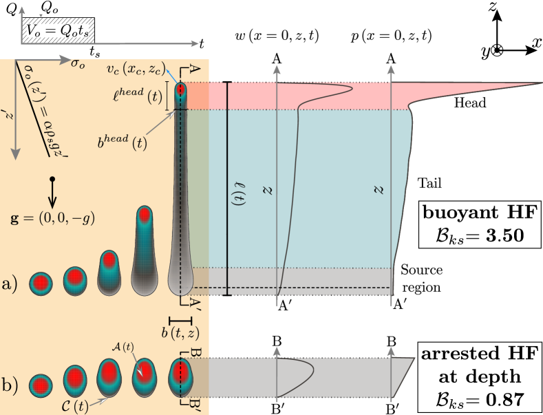
Figure 1: a) Buoyant self-sustained growth of a hydraulic fracture. b) Arrested hydraulic fracture at depth. Both fractures emerge from a finite fluid volume released from a point source through a block injection and propagate in a homogeneous linear elastic medium ($x|z$ plane) with the downwards oriented gravity vector ${\displaystyle\mathbf{g}}$ (in ${\displaystyle-z}$) creating a linear confining stress ${\displaystyle\sigma_{o}\left(z\right)}$. Fracture area is denoted by ${\displaystyle\mathcal{A}\left(t\right)}$ with a closed front ${\displaystyle\mathcal{C}\left(t\right)}$ and a local normal velocity ${\displaystyle v_{c}\left(x_{c},z_{c}\right)}$ (with ${\displaystyle\left({\displaystyle x_{c},}z_{c}\right)\in{\displaystyle\mathcal{C}\left(t\right)}}$). The fracture extent is defined by its local breadth ${\displaystyle b\left(z,t\right)}$ and total length ${\displaystyle\ell\left(t\right)}$.

2 Preliminaries

We investigate tensile (mode I) hydraulic fractures under the classical assumption of linear elastic fracture mechanics (LEFM) and laminar Newtonian lubrication flow (Detournay, 2016). The finite volume is released from a point source at depth into a linearly elastic and impermeable medium with uniform properties. The fracture orientation and stress state are equivalent to the one described in Möri & Lecampion (2022) and sketched in figure 1. We omit the detailed discussion of the mathematical formulation (see Möri & Lecampion (2022) for details) as the only difference pertains to the history of the fluid release.We consider here a simple injection history where the fluid volume is released at a constant rate until the end of the release at time $t=t_{s}$ (the shut-in time), where the rate suddenly drops to zero. We denote the constant release rate during the block injection as $Q_{o}$ such that the rate history is simply:

$$Q\left(t\right)=\begin{cases}Q_{o}&t\leq t_{s}\\ 0&t>t_{s}\end{cases}.$$ (1)

The coherent global volume balance in the case of an impermeable medium is

$$\mathcal{V}\left(t\right)=\int_{\mathcal{A}(t)}w\left(t,x,z\right)\text{d}x\text{d}z=\begin{cases}Q_{o}t&t<t_{s}\\ V_{o}=Q_{o}t_{s}&t\geq t_{s}\end{cases},$$ (2)

where $V_{o}=Q_{o}t_{s}$ is the total volume of fluid released.

In the following, we combine scaling arguments and numerical simulations using the fully-coupled planar 3-D hydraulic fracture solver PyFrac (Zia & Lecampion, 2020). We refer the reader to Zia & Lecampion (2020) and references therein for a detailed description of the numerical scheme. The documentation of the open-source code and examples of applications are available for download at PyFrac. The initial conditions and parameters used for the numerical simulations are detailed in section 2.2 of Möri & Lecampion (2022) as well as in the shared data of this article.

2.1 Arrest of a finite volume radial hydraulic fracture without buoyancy

In the absence of buoyant forces, considering the limiting case of an impermeable medium, hydraulic fractures finally arrest after the end of the injection when reaching an equilibrium between the injected volume and the linear elastic fracture mechanics propagation condition. This problem was investigated in Möri & Lecampion (2021). The fracture characteristics at arrest are independent of the shut-in time $t_{s}$. They only depend on the properties of the solid and the total amount of fluid released. For example, the arrest radius $R_{a}$ (subscript $a$ for arrest) is given by

$${\displaystyle R_{a}=\left(\frac{3}{8\sqrt{\pi}}\right)^{2/5}\left(\frac{E^{\prime}V_{o}}{K_{Ic}}\right)^{2/5}},$$ (3)

where $E^{\prime}=E/\left(1-\nu^{2}\right)$ is the plane-strain modulus with $E$ the materials Young’s modulus and $\nu$ its Poisson’s ratio, and ${\displaystyle K_{Ic}}$ the fracture toughness of the material.

Even though the arrest radius is independent of $t_{s}$, the growth history prior to arrest depends on it. In particular, the arrest is not necessarily immediate after the end of the release. This is notably the case when the hydraulic fracture propagates in the viscosity-dominated regime at the end of the release. The immediate arrest versus continuous growth is captured by the value of the dimensionless toughness at the shut-in time:

$$\mathcal{K}_{ms}=K_{Ic}\frac{t_{s}^{1/9}}{E^{\prime 13/18}\mu^{\prime 5/18}Q_{o}^{1/6}}.$$ (4)

where $\mu^{\prime}=12\mu$ and $\mu$ is the fracturing fluid viscosity. In (4), we have used the subscripts $m$ and $s$ to indicate respectively a viscous scaling and the end of the release. If the fracture is viscosity-dominated ( $\mathcal{K}_{ms}\ll 1$), it propagates in a viscosity-dominated pulse regime for a while until it finally arrests when reaching $R=R_{a}$. On the other hand, if fracture energy is already dominating ( $\mathcal{K}_{ms}\gg 1$), the arrest is immediate upon shut-in. The viscosity-dominated pulse regime has been shown to emerge for $\mathcal{K}_{ms}\lessapprox 0.3$ (for a detailed description of the viscosity-dominated pulse regime, see section 3.2 of Möri & Lecampion (2021)). A numerical estimation of the immediate arrest yields a value of $\mathcal{K}_{ms}\gtrapprox 0.8$ (note that Möri & Lecampion (2021) report a value of $2.5$ due to an alternative definition of (4) using $K^{\prime}=\sqrt{32/\pi}K_{Ic}$ instead of $K_{Ic}$).

2.2 Buoyant hydraulic fracture under a continuous release

In the case of a fluid release occurring at a constant volumetric rate $Q_{o}$, the fracture elongates in the direction of gravity in the presence of buoyant forces. Two dimensionless buoyancies related either to the viscosity dominated (subscript $m$) or the toughness-dominated regime (subscript $k$) emerge (Möri & Lecampion, 2022):

$$\mathcal{B}_{m}=\varDelta\gamma\frac{Q_{o}^{1/3}t^{7/9}}{E^{\prime 5/9}\mu^{\prime 4/9}},\quad\mathcal{B}_{k}=\varDelta\gamma\frac{E^{\prime 3/5}Q_{o}^{3/5}t^{3/5}}{K_{Ic}^{8/5}}.$$ (5)

These dimensionless buoyancies are related through the dimensionless viscosity of a radial fracture when buoyancy becomes of order $\mathcal{O}(1)$:

$$\mathcal{M}_{\widehat{k}}=\mu^{\prime}\frac{Q_{o}E^{\prime 3}\varDelta\gamma^{2/3}}{K_{Ic}^{14/3}}$$ (6)

as

$$\mathcal{B}_{k}=\mathcal{B}_{m}^{27/35}\mathcal{M}_{\widehat{k}}^{12/35}.$$ (7)

Similar to the dimensionless toughness at the end of the release $\mathcal{K}_{ms}$ (4), $\mathcal{M}_{\widehat{k}}$ defines if the transition from a radial to an elongated buoyant fracture occurs in the viscosity- ($\mathcal{M}_{\widehat{k}}\gg 1$) or toughness-dominated ($\mathcal{M}_{\widehat{k}}\ll 1$) phase of the radial hydraulic fracture propagation. A family of solutions emerges as a function of this dimensionless viscosity $\mathcal{M}_{\widehat{k}}$ as discussed in detail in Möri & Lecampion (2022). Notably, a limiting large toughness solution has been obtained in Garagash & Germanovich (2014) (see details in Garagash & Germanovich (2022)). This large toughness limit is observed for $\mathcal{M}_{\widehat{k}}\leq 10^{-2}$ (Möri & Lecampion, 2022) and shows a buoyant finger-like fracture with a constant breadth and a fixed-volume head. These attributes, combined with a constant injection rate, lead to a linear growth rate of the buoyant fracture. In an intermediate range of values for $\mathcal{M}_{\widehat{k}}\in\left[10^{-2},10^{2}\right]$, the fractures exhibit a uniform horizontal breadth and a finger-like shape. In this range of $\mathcal{M}_{\widehat{k}}$, the prefactors (for length, width etc.) become dependent on the dimensionless viscosity $\mathcal{M}_{\widehat{k}}$ (4). Particularly, an increase in fracture breadth and head volume is observed with increasing values of $\mathcal{M}_{\widehat{k}}$ . Even larger values of $\mathcal{M}_{\widehat{k}}\geq 10^{2}$ generate fractures exhibiting a negligible toughness, buoyant solution at intermediate times, where the growth of the fracture is sub-linear. The breadth of these fractures increases for a while before reaching an ultimately constant value in relation to the non-zero value of fracture toughness. The fracture’s growth rate then becomes constant. Concurrently, the head and tail structure stabilizes. In the strictly zero-toughness limit, the breadth continuously increases and the fracture height growth always remains sub-linear as a consequence of global volume balance.

2.3 Hydrostatically loaded radial fracture

The occurrence of the self-sustained buoyant growth of a finite volume fracture has been investigated by several authors from the point of view of the static linear elastic equilibrium of a radial fracture under a linearly varying load (Davis et al., 2020; Salimzadeh et al., 2020; Davis et al., 2023). Under the hypothesis of zero viscous flow, the net loading opening the fracture is equal to the hydrostatic fluid pressure minus the linearly varying background stress $\sigma_{o}\left(z\right)$. The elastic solution and the evolution of the stress intensity factor at the upper and lower tip are known analytically for this loading (Tada et al., 2000). Adopting a LEFM propagation condition, the stress-intensity factor (SIF) $K_{I}$ at the upper end is set to the material fracture toughness $K_{Ic}$. On the other hand, the lower tip SIF is set to zero, allowing the fracture to close and liberate the volume necessary for further upward propagation. Enforcing the conditions of $K_{I}=K_{Ic}$ at the upper and $K_{I}=0$ at the lower tip constrains the limiting volume to

$$V_{\textrm{limit}}\propto\frac{K_{Ic}^{8/3}}{E^{\prime}\varDelta\gamma^{3/5}}=V_{\widehat{k}}^{\textrm{head}}$$ (8)

This minimal volume for buoyant propagation has been independently identified in recent contributions (Davis et al., 2020; Salimzadeh et al., 2020; Davis et al., 2023). Interestingly, it corresponds to the volume $V_{\widehat{k}}^{\text{head}}$ of the toughness-dominated head of a buoyant hydraulic fracture in the case of a constant release (Garagash & Germanovich, 2014; Möri & Lecampion, 2022).

If the volume of fluid released in the radial fracture is slightly larger than this value, the upper tip would have a stress intensity $K_{I}>K_{Ic}$, indicating excess energy leading to upward propagation. Similarly, the lower end would have $K_{I}<0$ and hence pinch. Small perturbations of the released volume around this minimum would lead to either an arrest of the fracture (lower volume) or a departure of a buoyant fracture (larger volume). Note that when the fracture volume equals this minimal volume, and fluid viscosity is neglected, the previous derivation fails to predict how the fracture will subsequently propagate. Only the introduction of fluid viscosity can resolve the physical limitation of this approach.

In addition, the previous derivation of the minimum volume for the occurrence of a self-sustained propagation assumes a perfectly radial shape until the entire fluid volume has been released. This approach is equivalent to considering buoyant forces only after the emplacement of the total released fluid has finished. It does not cover the case where buoyant forces are non-negligible during the release. It is further unclear if it applies to the case where fracture growth continues after the end of the release while buoyant forces are still negligible.

3 Arrest at depth vs self-sustained propagation of buoyant hydraulic fractures

From the discussion of the arrest radius of a hydraulic fracture in the absence of buoyancy (see section 2.1) and the regimes of buoyant hydraulic fracture growth under a continuous release (see section 2.2), we can anticipate several scenarios with respect to the emergence of a self-sustained buoyant finite volume fracture. The transition towards buoyancy-driven growth can occur during the release of fluid or during the pulse propagation phase, when the propagation is viscosity-dominated at the end of the release. We investigate these different propagation histories in relation to the dimensionless buoyancies and dimensionless buoyant viscosity introduced in section 2 and discuss their relationship with the critical minimum volume (8).

3.1 Toughness-dominated at the end of the release

We first investigate the case where the fracture is toughness-dominated at the end of the release. In the absence of buoyancy, a constant fluid pressure establishes in the penny-shaped fracture which immediately stops at its arrest radius $R_{a}$ (see equation (3)). Due to the addition of buoyant effects, a linear pressure gradient develops and creates the configuration discussed above (see section 2.3). We anticipate that the total volume released must exceed $V_{\widehat{k}}^{\textrm{head}}$ (8) for a buoyant fracture to emerge. Neglecting the temporal evolution, the comparison $V_{o}/V_{\widehat{k}}^{\textrm{head}}$ is sufficient to assess the emergence of buoyant fractures. When considering a radial growth in time, the dimensionless buoyancy $\mathcal{B}_{k}\left(t\right)$ (5) indicates when buoyant forces become dominant. Estimating $\mathcal{B}_{k}\left(t\right)$ at the end of the release $t=t_{s}$, we obtain

$$\mathcal{B}_{ks}=\mathcal{B}_{k}\left(t=t_{s}\right)=\varDelta\gamma\frac{E^{\prime 3/5}Q_{o}^{3/5}t_{s}^{3/5}}{K_{Ic}^{8/5}}=\varDelta\gamma\frac{E^{\prime 3/5}V_{o}^{3/5}}{K_{Ic}^{8/5}}=\left(\frac{V_{o}}{V_{\widehat{k}}^{\textrm{head}}}\right)^{3/5}.$$ (9)

From this last relation (9), we see that the condition of a dimensionless buoyancy at the end of the release $\mathcal{B}_{ks}>1$ (under the hypothesis of a radial toughness-dominated fracture) is strictly equivalent to the condition of a released volume larger than the minimal volume for buoyant growth (8).

3.2 Viscosity-dominated at the end of the release $\mathcal{K}_{ms}\ll 1$

In contrast to toughness-dominated hydraulic fractures, radial viscosity-dominated fractures at the end of the release will continue to propagate in a viscous-pulse regime until they reach their arrest radius $R_{a}$ (3) (Möri & Lecampion, 2021). During that post-release propagation phase, the fracture may become buoyant and continue its growth as a result. In addition, we need to check if it remains buoyant when it is already so at the end of the release. This can be done by estimating the dimensionless buoyancy of a radial viscous fracture $\mathcal{B}_{m}\left(t\right)$ (5) at the end of the release $t=t_{s}$:

$$\mathcal{B}_{ms}=\mathcal{B}_{m}\left(t=t_{s}\right)=\varDelta\gamma\frac{Q_{o}^{1/3}t_{s}^{7/9}}{E^{\prime 5/9}\mu^{\prime 4/9}}=\varDelta\gamma\frac{V_{o}^{1/3}t_{s}^{4/9}}{E^{\prime 5/9}\mu^{\prime 4/9}}.$$ (10)

A value of $\mathcal{B}_{ms}\geq 1$ indicates that the fracture has already transitioned to buoyant propagation when the release stops and is already elongated. On the other hand, if ${\displaystyle\mathcal{B}_{ms}<1}$, buoyancy is not of primary importance at the end of the release, and the fracture still exhibits a radial shape.

3.2.1 Dominant buoyancy at the end of the release $\mathcal{B}_{ms}\geq 1$

In the case $\mathcal{B}_{ms}\geq 1$, the fracture is already buoyant at the end of the release. We must check if it remains buoyant or possibly arrests after the release ends. It is natural to compare the volume of the viscous head at the end of the release $V_{\widehat{m}}^{\textrm{head}}\left(t=t_{s}\right)$ to the limiting volume (equation (8)). The time-dependent volume of a viscous head is given in equation 5.6 of Möri & Lecampion (2022) and relates to equation (10) as

$$\mathcal{B}_{ms}=\left(\frac{V_{o}}{V_{\widehat{m}}^{\textrm{head}}\left(t=t_{s}\right)}\right)^{2/3}.$$ (11)

Using the relationship of equation (7), we obtain the following relation with the minimal limiting volume:

$$\frac{V_{o}}{V_{\widehat{k}}^{\textrm{head}}}=\left(\frac{V_{o}}{V_{\widehat{m}}^{\textrm{head}}\left(t=t_{s}\right)}\right)^{6/7}\mathcal{M}_{\widehat{k}}^{4/7}.$$

For a viscosity-dominated fracture, one necessarily has $\mathcal{M}_{\widehat{k}}\geq 1$ and to be buoyant at the end of the release, we necessarily have $V_{o}\geq V_{\widehat{m}}^{\textrm{head}}\left(t=t_{s}\right)$ as $\mathcal{B}_{ms}\geq 1$. As a result of the previous relations, we necessarily have $V_{o}\geq V_{\widehat{k}}^{\textrm{head}}$, respectively $\mathcal{B}_{ks}\geq 1$, and the volume released is larger than the minimum required for a toughness-dominated radial fracture subjected to a linear pressure gradient to become buoyant. After the release has ended, the viscous forces diminish in the head which ultimately becomes toughness-dominated. As a result, after the release, as buoyancy is of order one, the condition $\mathcal{B}_{ks}\geq 1$ is always satisfied and self-sustained buoyant growth will necessarily continue.

3.2.2 Viscosity-dominated fracture with negligible buoyant forces at the end of the release $\mathcal{B}_{ms}<1$

If buoyancy forces are negligible at the end of the release, and the propagation is viscosity-dominated (${\displaystyle\mathcal{B}_{ms}<1}$ and $\mathcal{K}_{ms}\ll 1$), the finite volume fracture will continue to grow radially in a viscous-pulse regime for a while before it finally arrests. In the presence of buoyant forces, it may be possible that buoyancy takes over as a driving mechanism before the fracture arrests. To incorporate such a possible growth history into the analysis, we use a dimensionless buoyancy in such a radial viscous pulse regime:

$$\mathcal{B}_{m}^{\left[V\right]}\left(t\right)=\varDelta\gamma\frac{V_{o}^{1/3}t^{4/9}}{E^{\prime 5/9}\mu^{\prime 4/9}}=\mathcal{B}_{ms}\left(t/t_{s}\right)^{4/9},$$ (12)

where the superscript $\left[V\right]$ indicates that the scaling is related to a finite volume release (replacing $Q_{o}$ by $V_{o}/t$ in the continuous release expression). From Möri & Lecampion (2021), we know that the radial viscous pulse fracture stops propagating when it becomes toughness-dominated. The corresponding time scale for which $\mathcal{\mathcal{K}}_{m}^{\left[V\right]}$ of a finite volume radial hydraulic fracture in the absence of buoyancy (see equation 10 of Möri & Lecampion (2021)) becomes of order one and the fracture arrests is given by

$$t_{mk}^{\left[V\right]}=\frac{E^{\prime 13/5}V_{o}^{3/5}\mu^{\prime}}{K_{Ic}^{18/5}}.$$ (13)

It is thus possible to check if buoyancy is of order one at this characteristic time of arrest by estimating the value of the dimensionless buoyancy $\mathcal{B}_{m}^{\left[V\right]}\left(t\right)$ (12) at $t=t_{mk}^{\left[V\right]}$:

$$\mathcal{B}_{m}^{\left[V\right]}\left(t=t_{mk}^{\left[V\right]}\right)=\varDelta\gamma\frac{E^{\prime 3/5}V_{o}^{3/5}}{K_{Ic}^{8/5}}=\left(\frac{V_{o}}{V_{\widehat{k}}^{\textrm{head}}}\right)^{3/5}=\mathcal{B}_{ks}.$$ (14)

Interestingly, this evaluation is strictly equivalent to the comparison of the limiting $V_{\widehat{k}}^{\textrm{head}}$ with the total released volume $V_{o}$ (see (9)). We conclude that regardless of the propagation history, the comparison of the released volume with the limiting volume for toughness-dominated buoyant growth is sufficient to characterize the emergence of a self-sustained buoyant hydraulic fracture. In what follows, we use the dimensionless buoyancy of a radial toughness-dominated finite volume hydraulic fracture $\mathcal{B}_{ks}$ to quantify the emergence of self-sustained growth ($\mathcal{B}_{ks}>1$). Similarly, the volume ratio $V_{o}/V_{\widehat{k}}^{\textrm{head}}=\mathcal{B}_{ks}^{5/3}$ could also be used.

3.3 Structure of the solution for a finite volume release

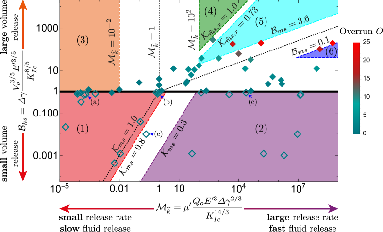
Figure 2: Structure of the solution for a finite volume release hydraulic fracture as a function of the dimensionless buoyancy $\mathcal{B}_{ks}$ (9) and viscosity ${\displaystyle\mathcal{M}_{\widehat{k}}}$ (6). Each symbol represents a simulation. Arrested fractures have empty symbols, filled symbols indicate self-sustained buoyancy-driven pulses. Numbered areas of different colours delimit distinct propagation histories. The colour of the symbols represents the value of the horizontal overrun $O$ (18). We indicate the simulations presented in figure 3 via blue arrows.

In the preceding subsections, the necessary and sufficient condition for the birth of a buoyant fracture $\mathcal{B}_{ks}\geq 1$ (see equation (9)) was derived. The fact that the birth (or not) of a buoyant hydraulic fracture solely depends on the total released volume and elastic parameters but is independent of how the volume is accumulated intrinsically derives from this statement. Furthermore, we discussed that the characteristics of self-sustained buoyant fractures depend additionally on the dimensionless viscosity $\mathcal{M}_{\widehat{k}}$ (see equation (6)), and hence on the specifics of the release (how the volume got released). These two parameters combined, encompass any possible configuration and thus form the parametric space of the entire problem (see figure 2).

First the parametric space can be split into an upper half ($\mathcal{B}_{ks}\geq 1$) where self-sustained buoyant propagation occurs and a lower part ($\mathcal{B}_{ks}<1$) where the fractures ultimately arrest at depth. We have numerically investigated this limit, where every symbol in figure 2 corresponds to a simulation. Empty symbols show simulations where the fracture ultimately arrests at depth, whereas filled symbols correspond to cases where self-sustained buoyant growth occurs. In general, figure 2 shows that the scaling argument that self-sustained buoyant growth occurs for $\mathcal{B}_{ks}\geq 1$ is correct without any prefactor. Only toughness-dominated fractures at the end of the release ($\mathcal{K}_{ms}\geq 0.8$ where no post-injection radial propagation occurs) sometimes lead to self-sustained buoyant growth for values of $\mathcal{B}_{ks}$ slightly smaller than 1. We use a value of $\mathcal{B}_{ks}=1$ as the limit for the birth of a self-sustained finite volume buoyant hydraulic fracture. This limit is close to the results obtained in previous contributions: $\mathcal{B}_{ks}\approx 0.90$ for Davis et al. (2020) and $\mathcal{B}_{ks}\approx 0.91$ for Salimzadeh et al. (2020). The equivalent value of $\mathcal{B}_{ks}$ calculated from the semi-analytically derived head volume of a propagating toughness-dominated buoyant fracture by Garagash & Germanovich (2014) is significantly higher: $\mathcal{B}_{ks}\approx 1.26$.

The parametric space of figure 2 captures more than the limit between fractures that ultimately arrest and self-sustained buoyant pulses.We distinguish six well-defined regions, corresponding to several limiting regimes of radial and buoyant growth: stagnant fractures with a toughness-dominated end of the release (region 1; bottom left - red, section 4), stagnant fractures with a viscosity-dominated end of the release (region 2; bottom right - purple, section 4), toughness-dominated buoyant fractures at the end of the release (region 3; top left - orange, section 5.1), viscosity-dominated buoyant fractures with a stabilized breadth at the end of the release (region 4; top centre - dark green, section 5.2.2), viscosity-dominated buoyant fractures without stabilization at the end of the release (region 5; top centre - light blue, section 5.2.1), and viscosity-dominated radial fractures at the end of the release (region 6; top right - dark blue, section 5.2.3). The distinction between regions 4 and 5 stems from the stagnation of lateral growth observed for viscosity-dominated buoyant hydraulic fractures under a constant release rate with a finite toughness (Möri & Lecampion, 2022) and will be detailed later.

4 Fractures arrested at depth $\mathcal{B}_{ks}<1$

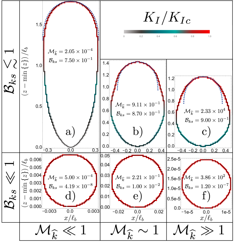
Figure 3: Final shape and stress intensity factors (SIF) along the front $\mathcal{C}\left(t\right)$ of ultimately arrested fractures at depth ($\mathcal{B}_{ks}<1$) as a function of $\mathcal{B}_{ks}$ and $\mathcal{M}_{\widehat{k}}$. Colours indicate the ratio between the local stress intensity factor $K_{I}$ and the material fracture toughness $K_{Ic}$ from 0 (light grey) to 1 (red). The blue dashed lines in a) to c) correspond to the shape of an expanding head of a propagating toughness-dominated buoyant fracture (Garagash & Germanovich, 2014).

Fractures which arrest at depth do not show self-sustained propagation in the buoyant direction. In the absence of any form of material or stress heterogeneities and assuming an infinite impermeable elastic medium, a fracture will arrest only if an insufficient volume is released: $\mathcal{B}_{ks}<1$. The lower part of figure 2 distinguishes two propagation histories for arresting fractures: a region where the fracture is toughness-dominated at the end of the release (region 1) and one where it is viscosity-dominated (region 2). As described in section 2.1, the characteristics of radially arresting fractures are independent of the propagation history. In the cases where $\mathcal{B}_{ks}\ll 1$, the fracture has a stress intensity factor (SIF) $K_{I}$ along the entire fracture front equal to the fracture toughness $K_{Ic}$ (c.f. figures 3d) - f)). In other words, as long as the final radius of the fracture $R_{a}$ (3) is small compared to the buoyancy length scale $\ell_{b}$ (Lister & Kerr, 1991), the fracture arrests radially, and the findings obtained in the absence of buoyancy are valid (Möri & Lecampion, 2021).

For larger released volumes which are still insufficient for the start of self-sustained growth ($\mathcal{B}_{ks}\lesssim 1$), fracture elongation occurs before it finally arrests. The fracture footprints of figures 3a) - c) indicate such elongated shapes as the dimensionless buoyancy approaches 1. In line with this, the stress intensity factor is smaller than the material toughness in the lower part of the fracture. The final elongation of the fracture is more pronounced for lower values of the dimensionless viscosity $\mathcal{M}_{\widehat{k}}$. The continuous release case has shown that toughness- and viscosity-dominated transitions present a distinct evolution of their shape (Möri & Lecampion, 2022). The different shapes of the arrested fractures as a function of the dimensionless viscosity when the released volume, approaches the limiting one is therefore not surprising.

5 Self-sustained finite volume buoyant fractures: $\mathcal{B}_{ks}>1$

5.1 Toughness-dominated, buoyant fractures at the end of the release (region 3): $\mathcal{M}_{k}\ll 1$

When the released volume is sufficient to create a buoyant hydraulic fracture ($\mathcal{B}_{ks}>1$), a set of possible propagation histories exists as function of the dimensionless viscosity $\mathcal{M}_{k}$. We first discuss toughness-dominated fractures which, according to the arguments of sections 2.1 and 3, must have a transition from radial to buoyant when the release is still ongoing. This results in a well-established, finger-like buoyant fracture with a constant volume, toughness-dominated head at the end of the release. The head characteristics in the case of a continuous release were obtained from the assumption that $\ell^{\textrm{head}}\left(t\right)\sim b^{\textrm{head}}\left(t\right)$ and elasticity, toughness, and buoyant forces are dominating. If we additionally restrict these derivations by the finiteness of the total release volume, the resulting length, opening, and pressure scales remain unchanged (see equations 4.1 of Möri & Lecampion (2021)) but a time-dependent dimensionless viscosity emerges

$$\mathcal{M}_{\widehat{k}}^{\left[V\right]}\left(t\right)=\mu^{\prime}\frac{V_{o}E^{\prime 3}\varDelta\gamma^{2/3}}{K_{Ic}^{14/3}t}=\mathcal{M}_{\widehat{k}}\frac{t_{s}}{t}.$$ (15)

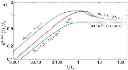
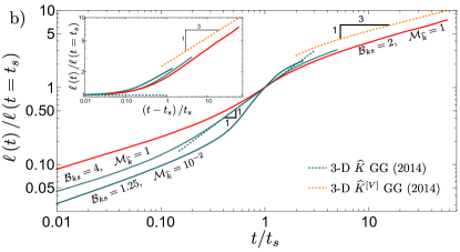
Figure 4: Toughness-dominated self-sustained buoyant fractures. Evolution of the dimensionless head breadth $b^{head}\left(t\right)/\ell_{b}$ (a) and fracture length $\ell\left(t\right)/\ell(t=t_{s})$ (b) as a function of the dimensionless shut-in time $t/t_{s}$. The green-dotted line corresponds to the limiting 3-D $\widehat{K}$ GG (2014) solution ($b^{head}\left(t\to\infty\right)=\pi^{-1/3}\ell_{b}$ in a), and the orange dashed line is the 3-D $\widehat{K}^{\left[V\right]}$ GG (2014) solution. The inset of figure (b) shows the same quantity on the y-axis with a shifted x-axis (e.g. $\left(t-t_{s}\right)/t_{s}$).

The decreasing nature of $\mathcal{M}_{\widehat{k}}^{\left[V\right]}$ with time indicates that the fracture head will necessarily become toughness-dominated at late time. Garagash & Germanovich (2014) similarly derived the finite volume limit and conclude that the head and tail breadth do not change compared to the continuous release case. Their solution is thus equivalently representative of any finite volume, buoyant hydraulic fracture with a finite toughness. We denote their result hereafter as the 3-D $\widehat{K}^{\left[V\right]}$ GG (2014) solution. For cases in the intermediate range of $\mathcal{M}_{\widehat{k}}\in\left[10^{-2},10^{2}\right]$, we check how their head breadth approaches the 3-D $\widehat{K}^{\left[V\right]}$ GG (2014) solution at late time (e.g. $b^{head}\left(t\to\infty\right)=\pi^{-1/3}\ell_{b}$). We show in figure 4a) the evolution of one toughness-dominated simulation with $\mathcal{M}_{\widehat{k}}=10^{-2}$ and two fractures with an intermediate value of $\mathcal{M}_{\widehat{k}}=1$. The head breadth of the toughness-dominated fracture validates the limiting solution during the release (dark green line in figure 4a)) and shows no change after the release has ended. In contrast to this constant value of the head breadth, the simulations with an intermediate value of $\mathcal{M}_{\widehat{k}}$ (light green and red lines in figure 4a)) have a maximum value exceeding the limiting breadth at the end of the release. Afterwards, the head breadth gradually reduces and approaches the limiting 3-D $\widehat{K}^{\left[V\right]}$ GG (2014) solution. In the continuous relese case, the limiting breadth is valid for $\mathcal{M}_{\widehat{k}}\leq 10^{-2}$, using equation (15) we can thus estimate the time for the fracture to reach the limit as $t\left(\mathcal{M}_{\widehat{k}}^{\left[V\right]}\left(t\right)=10^{-2}\right)=10^{2}\mathcal{M}_{\widehat{k}}t_{s}$ (Möri & Lecampion, 2022). For $\mathcal{M}_{\widehat{k}}\in\left[10^{-2},10^{2}\right]$, the simulations presented in figure 4 the 3-D $\widehat{K}^{\left[V\right]}$ GG (2014) solution would be reached once $t\sim 100t_{s}$. From the rate with which the breadth approaches the 3-D $\widehat{K}^{\left[V\right]}$ GG (2014) observed in figure 4a), this estimate seems reasonable. In fact, the fracture with $\mathcal{M}_{\widehat{k}}=1$ and $\mathcal{B}_{ks}=2$ is already within $15\%$ of the limiting solution at $t\sim 50t_{s}$.

We derive the scaling of the viscosity-dominated tail of such a late-time solution using the assumption of a constant frature breadth on the order of the breadth of the head $b\sim\ell_{b}=K_{Ic}^{2/3}/\varDelta\gamma^{2/3}$ as

$$\ell_{\widehat{k}}^{\left[V\right]}\left(t\right)=\frac{V_{o}^{2/3}\varDelta\gamma^{7/9}\,t^{1/3}}{K_{Ic}^{4/9}\mu^{\prime 1/3}},\quad b_{\widehat{k}}^{\left[V\right]}=\frac{K_{Ic}^{2/3}}{\varDelta\gamma^{2/3}}\equiv\ell_{b}$$ (16)

$$w_{\widehat{k}}^{\left[V\right]}\left(t\right)=\frac{V_{o}^{1/3}\mu^{\prime 1/3}}{K_{Ic}^{2/9}\varDelta\gamma^{1/9}t^{1/3}},\quad p_{\widehat{k}}^{\left[V\right]}\left(t\right)=E^{\prime}\frac{\varDelta\gamma^{5/9}V_{o}^{1/3}\mu^{\prime 1/3}}{t^{1/3}K_{Ic}^{8/9}}.$$ (17)

where we use $\widehat{\cdot}$ to refer to a buoyant scaling. These scales are obtained from the continuous release scales by replacing $Q_{o}$ with $V_{o}/t$, and reveal a sub-linear growth of the fracture height according to a power law of the form $\ell\left(t\right)\sim t^{1/3}$. Note that these scales have been obtained by Garagash & Germanovich (2014) when deriving their 3-D $\widehat{K}^{\left[V\right]}$ GG (2014) solution. We present in figure 4b) the evolution of dimensionless fracture length $\ell\left(t\right)/\ell\left(t=t_{s}\right)$ as a function of the dimensionless time $t/t_{s}$. The dark green line with a $1:1$ slope indicates the scaling derived temporal power-law for a toughness-dominated buoyant hydraulic fracture under a continuous fluid release. The two simulations with low $\mathcal{B}_{ks}$ (dark red and green) cannot reach this intermediate regime, as they are not propagating long enough in this $\widehat{K}$-regime (see the discussion in section 4.4 of Möri & Lecampion (2022)). The simulation with $\mathcal{B}_{ks}=4$ reaches this limit for about one order of magnitude in time before decelerating towards the late-time power law predicted by the scaling of equation (16). A similar deceleration is observed for the other two simulations without any of the simulations reaching the limitting $\ell\left(t\right)\sim t^{1/3}$ power-law. The orange dashed line indicates the 3-D $\widehat{K}^{\left[V\right]}$ GG (2014) for fracture length, which we would expect to be valid at late times. The inset of figure 4b) sets the time when the release ends as zero according to the hypothesis of Garagash & Germanovich (2014). This correction of the data highlights the tendency of the fracture length of all simulations to approach the limiting solution. A late-time validation of the solution can be expected as the relative difference between the predicted length and the simulation with $\mathcal{B}_{ks}=2$ and $\mathcal{M}_{\widehat{k}}=1$ at the end of the simulation is only on the order of $23\%$. These findings indicate that buoyant fractures with a finite toughness will have a late-time behaviour akin to the 3-D $\widehat{K}^{\left[V\right]}$ GG (2014) solution. Even though this late-time behaviour will be consistent, it also shows that the exact shape of the fracture will depend on both parameters, $\mathcal{M}_{\widehat{k}}$ and $\mathcal{B}_{ks}$. Only the breadth close to the head, the head itself, and the growth rate will be equivalent to the 3-D $\widehat{K}^{\left[V\right]}$ GG (2014) solution. To get an idea of the overall fracture shape, we define a shape parameter called the overrun as

$$O=\frac{\underset{z,t}{\text{max}}\left\{b\left(z,t\right)\right\}-\pi^{-1/3}\ell_{b}}{\pi^{-1/3}\ell_{b}}.$$ (18)

This parameter defines how much the maximum lateral extent exceeds the late-time head breadth $\pi^{-1/3}\ell_{b}$. $O$ has a lower bound of $0$, reached for fully toughness-dominated fractures with $\mathcal{M}_{\widehat{k}}\leq 10^{-2}$. This limit is validated by the simulation reported in this section with $\mathcal{M}_{\widehat{k}}=10^{-2}$ and $\mathcal{B}_{ks}=1.25$ which effectively has an overrun of $0.$ For the fractures in between the toughness and viscosity dominated limit of the continuous release with a uniform breadth (e.g. $\mathcal{M}_{\widehat{k}}\in\left[10^{-2},10^{2}\right]$), the overrun cannot be predicted by scaling laws. From the observation of figure 8 of Möri & Lecampion (2022), we can however derive that it will increase with increasing values of $\mathcal{M}_{\widehat{k}}$.The overrun of the two simulations reported here is respectively $0.88$ ($\mathcal{M}_{\widehat{k}}=1$ and $\mathcal{B}_{ks}=4$) and $0.80$ ($\mathcal{M}_{\widehat{k}}=1$ and $\mathcal{B}_{ks}=2$). We display the value of the overrun for simulations which lead to a buoyant hydraulic fracture in figure 2. Within the region of the toughness-dominated fractures with a buoyant end of the release (region 1), the values are effectively $0$. The overrun increases with the value of $\mathcal{M}_{\widehat{k}}$ towards the viscosity-dominated domain (regions 4 to 6) and will be estimated using scaling arguments later.

5.1.1 Numerical Limitations

The fact that no simulations propagating for longer times - which would ultimately exhibit the 3-D $\widehat{K}^{\left[V\right]}$ GG (2014) solution - are reported deserves discussion. These simulations have multiple numerical challenges: their overall computational cost and the numerical treatment of closing cells at the bottom of the fracture, among others. We illustrate the computational cost by the example of a toughness-dominated buoyant hydraulic fracture. Such fractures accelerate around the transition from radial to buoyant before slowing down to the ultimately constant velocity. Möri & Lecampion (2022) report that for their simulations, the acceleration terminates at a dimensionless time of approximately $t/t_{k\widehat{k}}\approx 3$, where $t_{k\widehat{k}}$ is the transition time from radial to buoyant (see equation 3.6 of Möri & Lecampion (2022)). Observation of figure 4b) shows that after the end of the release, additional time is required to transition to the late-time buoyant pulse solution. This figure gives an estimate of the time to reach the 3-D $\widehat{K}^{\left[V\right]}$ GG (2014) solution of $t\sim 100t_{s}$. An estimate of the fracture extent for a simulation with $\mathcal{M}_{\widehat{k}}=10^{-2}$ at this time, based on a growth according to the power law of equation (16), gives $\ell\sim 1600\ell_{b}$. The computational cost can now be estimated by taking a discretization of approximately $44$ elements per $\ell_{b}$ (see section 4.2 of Möri & Lecampion (2022)) and an approximation of the constant breadth of $b\left(t\right)\approx\pi^{-1/3}\ell_{b}$, yielding about $2\times 10^{6}$ elements in the fracture. Our current implementation of PyFrac (Zia & Lecampion, 2020) is able to handle buoyant simulations covering up to $20$ orders of magnitude in time and up to $15$ orders of magnitude in space within about $4$ weeks of computation time on a multithreaded Linux desktop system with twelve Intel®Core i7-8700 CPUs, using at most 30 GB of RAM, and arising to a discretization of up to $2\times 10^{5}$ elements within the fracture footprint.

An additional issue presents closing cells at the bottom of the fracture. As the opening continuously reduces (see $w_{\widehat{k}}^{\left[V\right]}$ in equation (16)) and we do not allow for complete fracture healing, a minimum width activates (Zia & Lecampion, 2020). From this arise two effects: First, elastic contact stress changes the stress distribution and the overall behaviour. Second, some volume gets trapped, reducing the one available for fracture propagation. The latter will artificially slow down propagation (Pezzulli, 2022) and ultimately arrest the fracture. Both phenomena increase the non-linearity of the system, such that convergence is challenging, which leads to a breakdown of the simulation at late time $t\gg t_{s}$.

5.2 Viscosity-dominated at the end of the release (regions 4 to 6): $\mathcal{M}_{k}\gg 1$

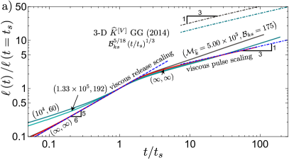
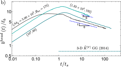
Figure 5: Evolution of fracture length $\ell\left(t\right)/\ell(t=t_{s})$ (a) and head breadth $b^{head}\left(t\right)/\ell_{b}$ for viscosity-dominated buoyant non-stabilized fractures at the end of the release as a function of the dimensionless shut-in time $t/t_{s}$: $\mathcal{M}_{\widehat{k}}\gg 1,\,\mathcal{B}_{ks}\geq 1,\,\mathcal{K}_{\widehat{m}x,s}<1$. Coloured dashed-dotted lines in (a) show the corresponding late-time, 3-D $\widehat{K}^{\left[V\right]}$ GG (2014) solution, the blue dashed line the continuous release buoyant scaling $\left(\ell\left(t\right)/\ell(t=t_{s})\sim t^{5/6}\right)$, the blue dashed-dotted line a numerical zero-toughness fit $\ell\left(t\right)/\ell\left(t=t_{s}\right)\approx 1.62\left(t/t_{s}\right)^{0.33}$ (matching the $\widehat{M}^{\left[V\right]}$-scaling). The green dashed line in (b) indicates the late-time limit of the 3-D $\widehat{K}$ GG (2014) solution for the corresponding simulation. The blue-dashed line indicates the scaling dependence in the $\widehat{M}^{\left[V\right]}$-scaling, $b^{head}\left(t\right)\sim t^{-1/6}$. Note that the two zero-toughness simulations differ by their value of $\mathcal{B}_{ms}$ ($100$ for the dark red and $25$ for the light red simulation).

The difference between a buoyant or radial end of the release has been shown to depend on the dimensionless viscosity at the end of the release $\mathcal{B}_{ms}$ (see equation (10), section 3.2). For an accurate evaluation of the emerging shape, an additional separation between two possible cases of buoyant fractures at the end of the release is required. Möri & Lecampion (2022) have shown that whenever a finite fracture toughness is present (e.g. $K_{Ic}\neq 0$), lateral growth stabilizes within a finite time at $\underset{z,t}{\text{max}}\left\{b\left(z,t\right)\right\}\propto\mathcal{M}_{\widehat{k}}^{2/5}\ell_{b}$. The time of stabilization is related to a dimensionless lateral toughness $\mathcal{K}_{\widehat{m},x}(t)$ (see their equation 6.1), which we can evaluate at the end of the release

$$\mathcal{K}_{\widehat{m}s,x}=\mathcal{K}_{\widehat{m},x}(t=t_{s})=K_{Ic}\frac{\varDelta\gamma^{1/8}\,t_{s}^{1/3}}{E^{\prime 19/24}V_{o}^{1/8}\mu^{\prime 1/3}}=\mathcal{M}_{\widehat{k}}^{1/3}\mathcal{B}_{ks}^{25/72}.$$ (19)

A value of $\mathcal{K}_{\widehat{m}s,x}\geq 1$ indicates that lateral growth has ceased, whereas a value below one means that the fracture is still growing laterally as $b\sim t^{1/4}$ (see equation 5.4 of Möri & Lecampion (2022)).

5.2.1 Viscosity-dominated, buoyant fracture at the end of the release without laterally stabilized breadth (region 5): $\mathcal{B}_{ms}\geq 1$ and$\mathcal{K}_{\widehat{m}s,x}\ll 1$

We consider first the case of zero-fracturing toughness by the development of a tail scaling. The principle hypotheses are buoyant forces, elasticity and viscous energy dissipation at first order and an aspect ratio scaling like the respective lateral and horizontal fluid velocities ($\ell\left(t\right)/b\left(t\right)\sim v_{z}\left(t\right)/v_{x}\left(t\right)$)

$$\ell_{\widehat{m}}^{\left[V\right]}=\frac{V_{o}^{1/2}\varDelta\gamma^{1/2}\,t^{1/3}}{E^{\prime 1/6}\mu^{\prime 1/3}},\quad b_{\widehat{m}}^{\left[V\right]}=\frac{E^{\prime 1/4}V_{o}^{1/4}}{\varDelta\gamma^{1/4}}$$ (20)

$$w_{\widehat{m}}^{\left[V\right]}=\frac{V_{o}^{1/4}\mu^{\prime 1/3}}{E^{\prime 1/12}\varDelta\gamma^{1/4}t^{1/3}},\quad p_{\widehat{m}}^{\left[V\right]}=\frac{E^{\prime 2/3}\mu^{\prime 1/3}}{t^{1/3}}.$$

Note that Davis et al. (2023) presented the same scaling for fracture length. The finite volume inherently prevents the infinite lateral growth observed for a continuous release and $b_{\widehat{m}}^{\left[V\right]}$ is time-independent. Figure 5c) shows limited lateral growth for all simulations. It is interesting to note, that the scaling predicts a fracture length evolution with a $\ell\sim t^{1/3}$ power-law, equivalent to the height evolution in the toughness-dominated case. Figure 5a) shows this evolution for various viscosity-dominated simulations. When $\mathcal{M}_{\widehat{k}}$ is sufficiently large and $\mathcal{K}_{\widehat{m}s}\ll 1$ (in other words when the fracture is sufficiently far from lateral stabilization) the $1:3$ slope predicted by the scaling of equation (20) emerges. However, the height growth quickly departs from the $t^{1/3}$ power-law. The reason is the time-dependent inflow rate of the head (derived from the scaling of equation (20))

$$\ell_{\hat{m}}^{head,\left[V\right]}=b_{\hat{m}}^{head,\left[V\right]}=\frac{E^{\prime 11/24}V_{o}^{1/8}\mu^{\prime 1/6}}{\varDelta\gamma^{5/8}t^{1/6}},\hskip 10.00002ptw_{\hat{m}}^{head,\left[V\right]}=\frac{V_{o}^{1/4}\mu^{\prime 1/3}}{E^{\prime 1/12}\varDelta\gamma^{1/4}t^{1/3}}$$ (21)

$$p_{\hat{m}}^{head,\left[V\right]}=\frac{E^{\prime 11/24}V_{o}^{1/8}\mu^{\prime 1/6}\varDelta\gamma^{3/8}}{t^{1/6}},\hskip 10.00002ptV_{\hat{m}}^{head,\left[V\right]}=\frac{E^{\prime 5/6}V_{o}^{1/2}\mu^{\prime 2/3}}{\varDelta\gamma^{3/2}t^{2/3}},$$

revealing a shrinking viscous head.

Considering now a finite fracture toughness, a dimensionless toughness can be obtained in the head

$$\mathcal{K}_{\widehat{m}}^{[V]}\left(t\right)=K_{Ic}\frac{t^{1/4}}{E^{\prime 11/16}V_{o}^{3/16}\varDelta\gamma^{1/16}\mu^{\prime 1/4}}=\mathcal{B}_{ks}^{5/48}\mathcal{M}_{\widehat{k}}^{[V]}\left(t\right)^{-1/4}=\mathcal{B}_{ks}^{5/48}\mathcal{M}_{\widehat{k}}^{-1/4}\left(\frac{t}{t_{s}}\right)^{1/4}.$$ (22)

Equation (22) indicates that the head will become toughness dominated at late times as $\mathcal{K}_{\widehat{m}}^{[V]}\left(t\right)$ increases with time. From this observation, we anticipate that the region close to the propagating head will ultimately follow the 3-D $\widehat{K}^{\left[V\right]}$ GG (2014) head solution (see section 5.1.1) and derive the characteristic time scale of the transition

$$t_{\widehat{m}\widehat{k}}^{[V]}=\frac{E^{\prime 11/4}V_{o}^{3/4}\varDelta\gamma^{1/4}\mu^{\prime}}{K_{Ic}^{4}}.$$ (23)

Evaluating the viscosity-dominated head scaling (see equations (21)) at this characteristic time gives the scales of the toughness-dominated head (see (16)). This observation implies that even though the shape further away from the head varies, the length scale $\ell\left(t\right)_{\widehat{k}}^{\left[V\right]}$ becomes applicable. Relating the two length scales of buoyant fractures from a finite volume release

$$\ell{}_{\widehat{k}}^{\left[V\right]}\left(t\right)=\mathcal{B}_{ks}^{5/18}\ell{}_{\widehat{m}}^{\left[V\right]}\left(t\right)$$ (24)

shows that $\ell{}_{\widehat{k}}^{\left[V\right]}\left(t\right)\geq\ell{}_{\widehat{m}}^{\left[V\right]}\left(t\right)$ for a buoyant fracture (as $\mathcal{B}_{ks}\geq 1$). The observation of figure 5a) shows the fracture deviation from the lower, viscosity-dominated solution towards the upper, toughness-dominated solution (shown by dashed-dotted lines for two simulations). The observed faster growth in height originates in the narrowingof the tail, creating a lateral inflow from the stagnant parts of the fracture into a central tube of the fixed breadth predicted by the 3-D $\widehat{K}^{\left[V\right]}$ GG (2014) solution. We do not present a simulation that finishes the transition to the toughness-dominated regime due to its excessive computational cost (see the discussion in section 5.1.1).

In equation (18), we have introduced the overrun as a characteristic of the fracture shape. In the case of viscous fractures with a buoyancy-dominated, laterally non-stabilized end of the release, such overrun can be estimated from the viscous scaling as

$$O_{\widehat{m}}=\frac{b_{\widehat{m}}^{\left[V\right]}-\pi^{-1/3}\ell_{b}}{\pi^{-1/3}\ell_{b}}=\pi^{1/3}\frac{E^{\prime 1/4}V_{o}^{1/4}\varDelta\gamma^{5/12}}{K_{Ic}^{2/3}}-1=\pi^{1/3}\mathcal{B}_{ks}^{5/12}-1.$$ (25)

The increase of the overrun with the value of the dimensionless buoyancy $\mathcal{B}_{ks}$ is observable in figure 2.

5.2.2 Viscosity-dominated, buoyant fracture at the end of the release with laterally stabilized breadth (region 4): $\mathcal{B}_{ms}\geq 1$ and $\mathcal{K}_{\widehat{m}s,x}\geq 1$

Lateral stabilization of buoyant, viscosity-dominated fractures occurs when the volume of the fracture head becomes constant, leading to two fixed points, the laterally stabilized breadth of $\underset{z,t}{\text{max}}\left\{b\left(z,t\right)\right\}\sim\mathcal{M}_{\widehat{k}}^{2/5}\ell_{b}$ and the constant volume, constant breadth head. The section of extending fracture breadth in between the two conserves its shape, creating a fracture where elongation concentrates within the zone of laterally stabilized breadth. From this observation, one can draw an analogy to a toughness-dominated buoyant fracture (see section 5.1). The scales of this equivalent toughness-dominated fracture are related through a factor of $\mathcal{M}_{\widehat{k}}^{2/5}$, such that the behaviour after the end of the release will be the same as presented in section 5.1, differing only by the starting point ($\mathcal{M}_{\widehat{k}}^{2/5}$ instead of $\mathcal{M}_{\widehat{k}}$).

Because the processes after the end of the release do not differ from toughness-dominated fractures, we omit a detailed discussion of this case hereafter and only list the difference in the shape parameter

$$O_{\widehat{m}}^{stab}=\frac{\mathcal{M}_{\widehat{k}}^{2/5}\ell_{b}-\pi^{-1/3}\ell_{b}}{\pi^{-1/3}\ell_{b}}=\pi^{1/3}\mathcal{M}_{\widehat{k}}^{2/5}-1.$$ (26)

The overrun in the non-stabilized case of viscosity-dominated fractures depends solely on the dimensionless buoyancy $\mathcal{B}_{ks}$ and, as such, on the total released volume and elastic parameters. In contrast, the governing parameter of the stabilized case is the dimensionless viscosity $\mathcal{M}_{\widehat{k}}$, and the history of the release (how the total volume gets accumulated) governs the overrun of the fracture.

5.2.3 Viscosity-dominated fracture with negligible buoyancy at the end of the release (region 6): $\mathcal{B}_{ms}\ll 1$

This type of fracture becomes buoyant in the pulse propagation phase as long as its dimensionless buoyancy $\mathcal{B}_{ks}$ (see (9)) is larger than one. This transition from radial to buoyant propagation is characterized by the dimensionless buoyancy of the viscous pulse $M^{\left[V\right]}$-scaling $\mathcal{B}_{m}^{\left[V\right]}\left(t\right)$ (see equation (12)) and has a characteristic transition time

$$t_{m\widehat{m}}^{\left[V\right]}=\frac{E^{\prime 5/4}\mu^{\prime}}{V_{o}^{3/4}\varDelta\gamma^{9/4}}=\mathcal{B}_{ks}^{-5/2}t_{\widehat{m}\widehat{k}}^{\left[V\right]}.$$ (27)

The corresponding transition length scale is equivalent to the constant breadth of a buoyant viscosity-dominated fracture $\ell_{m}^{\left[V\right]}\left(t=t_{m\widehat{m}}^{\left[V\right]}\right)=\ell_{m\widehat{m}}^{\left[V\right]}=b_{\widehat{m}}^{\left[V\right]}$, indicating that the maximum breadth is reached at the transition. Figure 6d) shows that for an increasing dimensionless buoyancy $\mathcal{B}_{ks}$ (see (9)), the growth of the maximal breadth continues (continuous lines) after transition but remains within the order of magnitude predicted by the scaling (20). Lateral growth ultimately tapers off at about $3\ell_{m\widehat{m}}^{\left[V\right]}$ at $t\approx 10^{3}t_{m\widehat{m}}^{\left[V\right]}$. The expected overrun becomes equivalent to the case of a non-stabilized, buoyant viscosity-dominated end of the release (see equation (25)).

The scaling for these fractures is given by equations (20) and (21). Despite the distinct propagation histories, the late-time fracture footprint does not vary significantly (see figure 7). Similar to the case of a constant release, the fracture first becomes somewhat elliptical with a peak in pressure and opening appearing in the fracture head. Propagation then deviates to the buoyant direction with a continuously shrinking head, and no saddle point develops between the maximum lateral extent and the head. In the case of finite fracture toughness, an inflexion point forms in this area, such that the evolution of the breadth towards the head becomes convex at the transition time $t_{\widehat{m}\widehat{k}}^{[V]}$ (see equation (23)). Note that the bottom end of the fractures in figure 6h), i) seem to be of uniform opening. This is a direct consequence of the numerical scheme where the minimum width was activated.

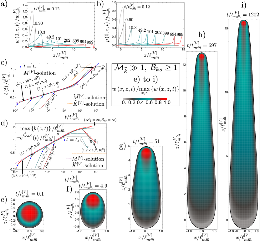
Figure 6: Viscosity-dominated, fractures with negligible buoyancy at the end of the release: $\mathcal{B}_{ks}\geq 1$ and $\mathcal{B}_{ms}\ll 1$. a) Opening along the centerline $w\left(0,z,t\right)/w_{m\widehat{m}}^{\left[V\right]}$ for $\mathcal{M}_{\widehat{k}}=\infty,\,\mathcal{B}_{ks}=\infty,$ and $\mathcal{B}_{ms}=10^{-3}$ (zero-toughness case). b) Net pressure along the centerline $p\left(0,z,t\right)/p_{m\widehat{m}}^{\left[V\right]}$ for the same case as in a). c) Fracture length $\ell\left(t\right)/\ell_{m\widehat{m}}^{\left[V\right]}$ for large viscosity $\mathcal{M}_{\widehat{k}}\in\left[5.1\times 10^{5},\infty\right]$ simulations. The blue dashed line is a fit of the zero-toughness simulation $\ell\left(t\right)\propto t^{0.33}$. d) Fracture breadth $b\left(t\right)/\ell_{m\widehat{m}}^{\left[V\right]}$ (continuous lines) and head breadth $b^{head}\left(t\right)/\ell_{m\widehat{m}}^{\left[V\right]}$ (dashed lines) for the same simulations. Purple dashed lines indicate the $M^{\left[V\right]}$-solution (Möri & Lecampion, 2021), orange dashed lines the 3-D $\widehat{K}^{\left[V\right]}$ GG (2014) solution for the highest value of $\mathcal{B}_{ks}$. e - i) Evolution of the fracture footprint from radial e) towards the late time shape h) and i)) for the zero-toughness simulation. For the definition of the transition scales $\cdot_{m\widehat{m}}^{\left[V\right]}$ see table 3.

When observing the evolution of the fracture length and head breadth, one observes that the simulations approach the 3-D $\widehat{K}^{\left[V\right]}$ GG (2014) solution for cases with a finite toughness. The breadth and length evolution of the 3-D $\widehat{K}^{\left[V\right]}$ GG (2014) in the viscous buoyant scaling (see equations (20) and (21)) depends on the value of $\mathcal{B}_{ks}$ such that we only indicate one of the possible late-time solutions. We pick the one which is most likely to be reached, corresponding to the smallest value of $\mathcal{B}_{ks}$ for the length and the largest for the breadth with dashed orange lines. The tendency towards those solutions is visible, reaching them exactly is however associated with too high computational costs (see the discussion in section 5.1.1). The evolution of fracture opening and net pressure is plotted along the centerline (e.g. $x=0$) in figures 6a) and b). The head is identified once it departs from the source before it subsequently shrinks. This shrinking makes the volume in the head become negligible in comparison to the overall fluid volume after sufficient buoyant propagation. When this moment is reached, the fracture propagates in the viscosity-dominated regime (see also the nearly self-similar footprint reported in the Supplementary Material). We show in the supplementary material that the opening along the centerline approaches the 2-D solution of Roper & Lister (2005). An approximated solution may be possible when combining the zero toughness head (c.f. figure 7 of Möri & Lecampion (2022)) with the tail solution of Roper & Lister (2007) (see their equation 6.7), but is left for further study.

5.3 Late time fracture shapes

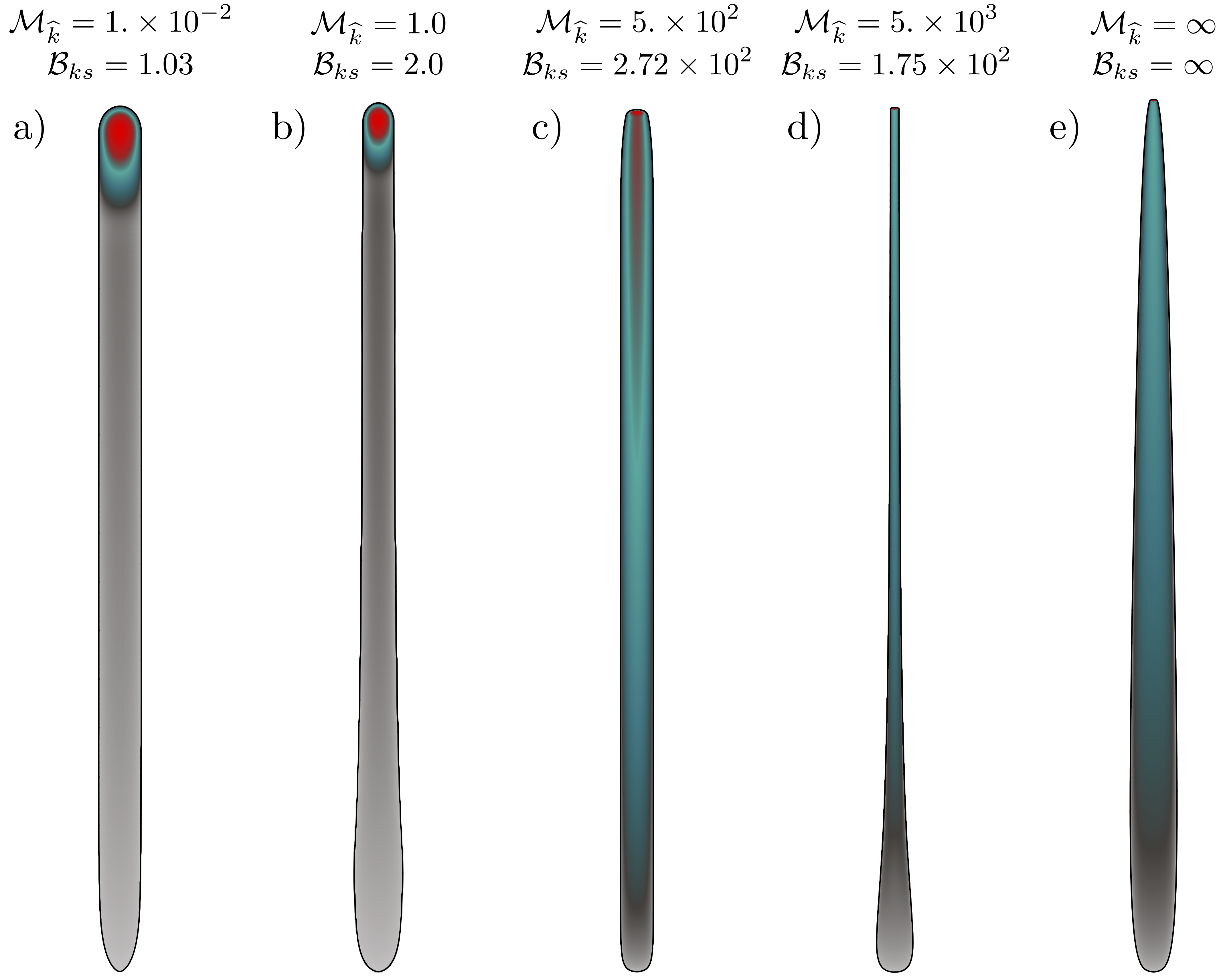
Figure 7: Phenotypes of possible buoyant hydraulic fractures of finite volume emerging from a point source $\left(\mathcal{B}_{ks}\geq 1\right)$. a) Toughness-dominated finger-like fracture (region 3 in figure 1). b) Intermediate fracture with a stable breadth and negligible overrun. c) Viscosity-dominated buoyant end of the release with stabilized breadth (region 4 in figure 1). d) Viscosity-dominated buoyant end of the release without stabilized breadth (region 5 in figure 1). e) Zero-toughness case with a buoyant end of the release $\left(\mathcal{B}_{ms}=10^{2}\right)$. a) and b) are scaled by $\ell_{b}$ (Lister & Kerr, 1991), c) to e) by $\ell_{m\widehat{m}}^{\left[V\right]}$ (see table 3).

The governing mechanisms delimiting the different regions of the parametric space of figure 2 give rise to different phenotypes of fracture shape. Figure 7 displays the late-time shape of buoyant fractures in the different regions (3-5) of the parametric space. Figure 7a) shows the characteristic shape of a toughness-dominated buoyant fracture at the end of the release (region 3). Their footprint is finger-like with a constant breadth and head volume. Already early in the propagation, the bulk of the released volume is located in the head (indicated by the colour code). Except in the source region and for the expanding head, no change in breadth is observed, and the overrun $O$ (see equation (18)) is zero. For fractures with a uniform breadth, not validating the toughness solution (e.g. $\mathcal{M}_{\widehat{k}}\in\left[10^{-2},10^{2}\right]$ and $\mathcal{B}_{ks}\geq 1$, between regions 3 and 4), the bulk of the fluid volume is similarly in the head. One difference is the change in breadth observed close to the source region related to the end of the release, giving rise to a small, non-zero overrun. When the fractures are more viscosity-dominated (see figures 7c-e)), the overrun becomes more pronounced, and the opening distribution is more homogeneous along the fracture length. For example, figure 7c) shows a viscosity-dominated, buoyant fracture with a stabilized breadth at the end of the release (region 4) with a barely visible head (light red area at the propagating edge). The red-coloured part extending long into the tail shows that the tail opening is much closer to the head opening than in the toughness-dominated cases of figures 7a) and b). The particularity of this phenotype is its uniform breadth over a finite height due to lateral stabilization (associated with a finite value of fracture toughness). Figure 7d) (region 5) emphasizes the approaching towards the late-time 3-D $K^{\left[V\right]}$ GG (2014) solution of viscosity-dominated fractures by the thinning of the breadth along the fracture length towards its head. The head breadth of this simulation still exceeds the limiting solution by a factor of about $4.7$ and the opening distribution along the fracture is still too homogeneous. In other words, a significant proportion of the volume remains in the tail (compare the grey colour in figure 7a) with the green colour in figure 7d)). The last phenotypein figure 7e), represents the case of a zero-toughness simulation with a buoyant end of the release. Comparing this shape to the zero toughness simulation with negligible buoyancy at the end of the release (c.f. figures 6h-i)) reveals no significant difference. All zero-toughness simulations, independent of the state at the end of the release, will show this particular shape. Only if a finite fracture toughness is present, the fracture will tend to the late-time 3-D $K^{\left[V\right]}$ GG (2014) solution and the shape will resemble figure 7d) (see also figure 1b) of Davis et al. (2023)).

6 Discussion

	Unit	Exp. 1837	Exp. 1945	Exp. 1967
$\mu_{f}$	$\textrm{Pa}\cdot\textrm{s}$	${\displaystyle 1.74\times 10^{-3}}$	${\displaystyle 48\times 10^{-3}}$	${\displaystyle 970\times 10^{-3}}$
$E$	Pa	$1345$	${\displaystyle 426}$	${\displaystyle 944}$
$\nu$		$0.5$	$0.5$	$0.5$
$K_{Ic}$	$\textrm{Pa}\cdot\textrm{m}^{1/2}$	${\displaystyle 23.1}$	$7.3$	${\displaystyle 16.2}$
$\varDelta\rho$	$\textrm{kg}\cdot\textrm{m}^{-3}$	${\displaystyle 260}$	${\displaystyle 160}$	${\displaystyle 150}$
$V_{o}$	$\textrm{m}^{3}$	${\displaystyle 2.\times 10^{-5}}$	${\displaystyle 1.\times 10^{-5}}$	${\displaystyle 1.\times 10^{-5}}$
$Q_{o}$	$\textrm{m}^{3}\cdot\textrm{s}^{-1}$	${\displaystyle 1.23\times 10^{-7}}$	$8.33\times 10^{-7}$	${\displaystyle 1.11\times 10^{-7}}$
$t_{s}$	s	$162$	${\displaystyle 12}$	${\displaystyle 90}$
$\mathcal{M}_{\widehat{k}}$		$1.20\times 10^{-3}$	$1.11$	$0.76$
$\mathcal{B}_{ks}$		$2.28$	$2.93$	$1.24$
$\mathcal{B}_{ms}$		$57.7$	$3.85$	$1.49$

Table 1: Material parameters and the released volume $V_{o}$ are taken from table 3 of Davis et al. (2023) (based on the work of Smitarello (2019)). We extract the shut-in time from figure 5a of Davis et al. (2023) and calculate the release rate as $Q_{o}=V_{o}/t_{s}$.

We compare recent laboratory experiments with our scalings and numerical simulations. We use three sets of parameters from experiments performed by Smitarello (2019) and reported in Davis et al. (2023) (see table 1). The resulting dimensionless parameters are listed in table 1. It appears that these fractures are either toughness-dominated (experiment 1827) or in the transition with a uniform breadth (experiments 1945 and 1967). We report the evolution of fracture height with time in figure 8 (data of the experiments from figure 5a of Davis et al. (2023)). Along with the three experiments, we show our simulation closest to experiments 1945 and 1967 as well as the limiting solutions derived by Garagash & Germanovich (2014). The toughness-dominated experiment (exp. 1837) display a linear fracture height growth with time, expected from the continuous release scaling. Surprisingly, the end of the release does not lead to a significant reduction in height growth (c.f. the simulation with $\mathcal{M}_{\widehat{k}}=10^{-2}$ in figure 4b)), which continues linearly until it reaches the top of the tank (end of the data stream). We expect this to be related to free-surface effects attracting the fracture, a hypothesis supported by observations of the other two experiments. The fractures of the other experiments grow without showing any scaling-based power laws. This behaviour is typical for many laboratory experiments which unfortunately appear to be “in-between” limiting regimes. Additionally, the extent of the hydraulic fractures created often suffers from detrimental effects associated with the finite size of the sample, making any comparison with theoretical and numerical predictions difficult. The fact that the release rate in laboratory experiments is often not constant, presents an additional inconvenience. Especially in viscosity-dominated fracture propagation regimes, this has a significant influence on fracture growth via $\mathcal{M}_{\widehat{k}}$.

The complete parametric space characterising 3-D finite volume buoyant hydraulic fractures described in this paper should help in better designing experiments within probing well-defined propagation history.

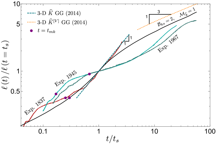
Figure 8: Fracture height evolution as a function of dimensionless time for the experiments listed in table 1. Data extracted from figure 5a of Davis et al. (2023) based on experiments reported in Smitarello (2019). The black line shows a simulation with similar dimensionless parameters to Exp. 1945 and Exp. 1967. Purple dots mark the moment when the fracture becomes toughness dominated (e.g. $t=t_{mk}$), and dashed lines indicate the limiting solutions derived by Garagash & Germanovich (2014) respectively (green for a continuous release, orange for the release of a finite volume).

7 Conclusions

We have shown that finite-volume hydraulic fractures are entirely characterized by a dimensionless buoyancy $\mathcal{B}_{ks}=\varDelta\gamma E^{\prime 3/5}V_{o}^{3/5}/K_{Ic}^{8/5}$ relating the total released $V_{o}$ to the minimum volume necessary for self-sustained buoyant propagation $V_{\widehat{k}}^{head}=K_{Ic}^{8/3}/\left(E^{\prime}\varDelta\gamma^{3/5}\right)$: $\mathcal{B}_{ks}=\left(V_{o}/V_{\widehat{k}}^{\textrm{head}}\right)^{3/5}$ and a dimensionless viscosity $\mathcal{M}_{\widehat{k}}=\mu^{\prime}Q_{o}E^{\prime 3}\varDelta\gamma^{2/3}/K_{Ic}^{14/3}$. Although the emergence (or not) of a self-sustained buoyant fracture solely depends on $\mathcal{B}_{ks}$, in other words, on the total volume released and material and fluid parameters, the details of the release (duration and injection rate) have a first order impact on the shape and propagation rates of the fracture through the dimensionless viscosity $\mathcal{M}_{\widehat{k}}$. Combining these two dimensionless numbers $(\mathcal{B}_{ks},\,\mathcal{M}_{\widehat{k}})$, reveals six regions corresponding to distinct propagation histories (see figure 2).

For a finite value of the material fracture toughness ($K_{Ic}\neq 0$), the toughness-dominated pulse solution of Garagash & Germanovich (2014) characterizes the late-time buoyant head and the fracture breadth in its vicinity ( $b^{head}=\pi^{-1/3}\ell_{b}$). Note that such a late-time solution may appear only at very late times. In the zero-toughness case ($K_{Ic}=0$), the fracture head shrinks eternally, and the maximum lateral breadth stabilizes at a finite value. It is thus possible to relate the limiting breadth close to the head to the stabilized maximum one. We define this parameter as the overrun $O$ and derive its value for the different regions of the parametric space. Note that this parameter gives only an idea of the shape: a similar overrun does not imply that the fracture has the same overall shape. When the fracturing toughness is zero, the head breadth tends to zero (e.g. $\ell_{b}=0\to b^{head}=0$), resulting in an infinite overrun. It is important to note that this does not imply unbounded lateral growth, as lateral growth is limited by the finite volume rather than fracture toughness.

The identified late-time behaviour further fixes the late-time ascent rate to the toughness-dominated solution as $\dot{\ell}_{\widehat{k}}^{\left[V\right]}\left(t\right)\sim V_{o}^{2/3}\varDelta\gamma^{7/9}/\left(K_{Ic}^{4/9}\mu^{\prime 1/3}t^{2/3}\right)\propto t^{1/3}$ . An important observation is that the time power-law dependence of the ascent rate for a viscosity-dominated buoyant fracture is equivalent (e.g. $\dot{\ell}_{\widehat{m}}^{\left[V\right]}\sim V_{o}^{1/2}\varDelta\gamma^{1/2}/\left(E^{\prime 1/6}\mu^{\prime 1/3}t^{2/3}\right)\propto t^{1/3}$). During its history, a buoyant hydraulic fracture can first ascent in a viscosity-dominated manner as $\dot{\ell}_{\widehat{m}}^{\left[V\right]}\left(t\right)$ and then transition to the limiting ascent rate dictated by the late toughness solution $\dot{\ell}_{\widehat{k}}^{\left[V\right]}\left(t\right)$. The late-time ascent rate of the toughness limit is always faster (or at least equal) than the one of the viscosity-dominated limit ($\dot{\ell}{}_{\widehat{k}}^{\left[V\right]}\left(t\right)=\mathcal{B}_{ks}^{5/18}\dot{\ell}{}_{\widehat{m}}^{\left[V\right]}\left(t\right)$, with $\mathcal{B}_{ks}\geq 1$ for a self-sustained buoyant fracture). Fractures transitioning when the fluid release is still ongoing can show even higher velocities during their propagation history. Estimations or averaging of vertical growth rates must be done with great care and must necessarily account for both $\mathcal{M}_{\widehat{k}}$ and $\mathcal{B}_{ks}$. In other words, both the details of the release history (rate and duration) do significantly impact the ascent rate even long after the end of the release. This implies that for realistic cases (as well as laboratory experiments), the detail of the released matter such that a more complicated evolution of the release (compared to the simple constant rate / finite duration) will certainly impact the growth of buoyant fractures.

It is noteworthy that most parameter combinations for natural or anthropogenic hydraulic fractures would lead to self-sustained buoyant propagation between the well-distinct regions of the parametric space depicted in 2. Additionally, the time required to reach the late-time solution at the propagating edge and the fracture size when doing so naturally clash with sample sizes in the laboratory or the scales of heterogeneities in the upper lithosphere. We emphasize that even though theoretically buoyant fractures emerge, nearly no cases of buoyant fractures from hydraulic fracturing treatments reaching the surface have been reported to our knowledge. We expect this contradiction to be related to the interaction of the growing fracture with heterogeneities, fluid leak-off, and other possible arrest mechanisms not accounted for in this contribution. Accounting for these effects is part of ongoing work and should elucidate why fractures ultimately arrest at depth, even when $\mathcal{B}_{ks}$ is above unity.

Acknowledgements. The authors gratefully acknowledge in-depth discussions with Dmitry Garagash.
Funding. This work was funded by the Swiss National Science Foundation under grant #192237.
Declaration of Interest. The authors report no conflict of interest.
Data availability statement. The data that support the findings of this study are openly available at 10.5281/zenodo.7788051 .
Author ORCID. A. Möri, 0000-0002-7951-1238; B. Lecampion, 0000-0001-9201-6592
Author contributions. Andreas Möri: Conceptualization, Methodology, Formal analysis, Investigation, Software, Validation, Visualization, Writing - original draft. Brice Lecampion: Conceptualization, Methodology, Formal analysis, Validation, Supervision, Funding acquisition, Writing - review & editing.

Appendix A Recapitulating tables of scales

For completeness, we list all the characteristic scales used within this contribution in the following tables. A Wolfram mathematica notebook containing their derivation and the different scalings is also provided as supplementary material.

	Radial		Elongated
	$\text{M}^{\left[V\right]}$	$\text{K}^{\left[V\right]}$	$\widehat{\text{M}}^{\left[V\right]}$ (tail)	$\widehat{\text{M}}^{\left[V\right]}$ (head)	$\widehat{\text{K}}^{\left[V\right]}$ (tail)	$\widehat{\text{K}}^{\left[V\right]}$ (head)
$\ell_{*}^{\left[V\right]}$	$\dfrac{E^{\prime 1/9}V_{o}^{1/3}t^{1/9}}{\mu^{\prime 1/9}}$	$\dfrac{E^{\prime 2/5}V_{o}^{2/5}}{K_{Ic}^{2/5}}$	$\dfrac{V_{o}^{1/2}\varDelta\gamma^{1/2}t^{1/3}}{E^{\prime 1/6}\mu^{\prime 1/3}}$	$\dfrac{E^{\prime 11/24}V_{o}^{1/8}\mu^{\prime 1/6}}{\varDelta\gamma^{5/8}t^{1/6}}$	$\dfrac{V_{o}^{2/3}\varDelta\gamma^{7/9}t}{K_{Ic}^{4/9}\mu^{\prime 1/3}}$	$\ell_{b}$
$b_{*}^{\left[V\right]}$	$\ell_{*}^{\left[V\right]}$	$\ell_{*}^{\left[V\right]}$	$\dfrac{E^{\prime 1/4}V_{o}^{1/4}}{\varDelta\gamma^{1/4}}$	$\ell_{*}^{head,\left[V\right]}$	$\ell_{b}=\dfrac{K_{Ic}^{2/3}}{\varDelta\gamma^{2/3}}$	$\ell_{*}$
$w_{*}^{\left[V\right]}$	$\dfrac{V_{o}^{1/3}\mu^{\prime 2/9}}{E^{\prime 2/9}t^{2/9}}$	$\dfrac{K_{Ic}^{4/5}V_{o}^{1/5}}{E^{\prime 4/5}}$	$\dfrac{V_{o}^{1/4}\mu^{\prime 1/3}}{E^{\prime 1/12}\varDelta\gamma^{1/4}t^{1/3}}$	$w_{*}^{tail,\left[V\right]}$	$\dfrac{V_{o}^{1/3}\mu^{\prime 1/3}}{K_{Ic}^{2/9}\varDelta\gamma^{1/9}t^{1/3}}$	$\dfrac{K_{Ic}^{4/3}}{E^{\prime}\varDelta\gamma^{1/3}}$
$V_{*}^{\left[V\right]}$	$V_{o}$	$V_{o}$	$V_{o}-V_{*}^{head,\left[V\right]}$	$\dfrac{E^{\prime 5/6}V_{o}^{1/2}\mu^{\prime 2/3}}{\varDelta\gamma^{3/2}t^{2/3}}$	$V_{o}-V_{*}^{head,\left[V\right]}$	$\dfrac{K_{Ic}^{8/3}}{E^{\prime}\varDelta\gamma^{5/3}}$
$p_{*}^{\left[V\right]}$	$\dfrac{E^{\prime 2/3}\mu^{\prime 1/3}}{t^{1/3}}$	$\dfrac{K_{Ic}^{6/5}}{E^{\prime 1/5}V_{o}^{1/5}}$	$\dfrac{E^{\prime 2/3}\mu^{\prime 1/3}}{t^{1/3}}$	$\dfrac{E^{\prime 11/24}V_{o}^{1/8}\mu^{\prime 1/6}\varDelta\gamma^{3/8}}{t^{1/6}}$	$\dfrac{E^{\prime}\varDelta\gamma^{5/9}V_{o}^{1/3}\mu^{\prime 1/3}}{K_{Ic}^{8/9}t^{1/3}}$	$K_{Ic}^{2/3}\varDelta\gamma^{1/3}$
$\mathcal{P}_{s}^{\left[V\right]}$	$\mathcal{K}_{m}^{\left[V\right]}=(t/t_{mk}^{\left[V\right]})^{5/18}$	$\mathcal{M}_{k}^{\left[V\right]}=(t/t_{mk}^{\left[V\right]})^{-1}$	$\mathcal{K}_{\widehat{m}}^{\left[V\right]}=\left(\mathcal{M}_{\widehat{k}}^{\left[V\right]}\right)^{-1/4}\mathcal{B}_{ks}^{5/48}$		$\mathcal{M}_{\widehat{k}}^{\left[V\right]}=\mu^{\prime}\dfrac{V_{o}E^{\prime 3}\varDelta\gamma^{2/3}}{K_{Ic}^{14/3}t}$
	$\mathcal{B}_{m}^{\left[V\right]}=(t/t_{m\widehat{m}}^{\left[V\right]})^{4/9}$	$\mathcal{B}_{k}^{\left[V\right]}=\varDelta\gamma\dfrac{E^{\prime 3/5}V_{o}^{3/5}}{K_{Ic}^{8/5}}$

Table 2: Characteristic scales (and governing dimensionless parameters) in the different scalings.

	$t^{\left[V\right]}$	$\ell_{*}^{\left[V\right]}=b_{*}^{\left[V\right]}$	$w_{*}^{\left[V\right]}$	$p_{*}^{\left[V\right]}$
$\text{M}^{\left[V\right]}\rightarrow\text{K}^{\left[V\right]}$	$t_{mk}^{\left[V\right]}=\dfrac{E^{\prime 13/5}V_{o}^{3/5}\mu^{\prime}}{K_{Ic}^{18/5}}$	$\ell_{mk}^{\left[V\right]}=\dfrac{E^{\prime 2/5}V_{o}^{2/5}}{K_{Ic}^{2/5}}$	$w_{mk}^{\left[V\right]}=\dfrac{K_{Ic}^{4/5}V_{o}^{1/5}}{E^{\prime 4/5}}$	$p_{mk}^{\left[V\right]}=\dfrac{K_{Ic}^{6/5}}{E^{\prime 1/5}V_{o}^{1/5}}$
$\text{M}^{\left[V\right]}\rightarrow\widehat{\text{M}}^{\left[V\right]}$	$t_{m\widehat{m}}^{\left[V\right]}=\dfrac{E^{\prime 5/4}\mu^{\prime}}{V_{o}^{3/4}\varDelta\gamma^{9/4}}$	$\ell_{m\widehat{m}}^{\left[V\right]}=\dfrac{E^{\prime 1/4}V_{o}^{1/4}}{\varDelta\gamma^{1/4}}$	$w_{m\widehat{m}}^{\left[V\right]}=\dfrac{V_{o}^{1/2}\varDelta\gamma^{1/2}}{E^{\prime 1/2}}$	$p_{m\widehat{m}}^{\left[V\right]}=E^{\prime 1/4}V_{o}^{1/4}\varDelta\gamma^{3/4}$
$\widehat{\text{M}}^{\left[V\right]}\rightarrow\text{$\widehat{\text{K}}$}^{\left[V\right]}$ (tail)	$t_{\widehat{m}\widehat{k}}^{\left[V\right]}=\dfrac{E^{\prime 11/4}V_{o}^{3/4}\varDelta\gamma^{1/4}\mu^{\prime}}{K_{Ic}^{4}}$	$\ell_{\widehat{m}\widehat{k}}^{\left[V\right]}=\dfrac{E^{\prime 1/4}V_{o}^{1/4}}{\varDelta\gamma^{1/4}}$	$w_{\widehat{m}\widehat{k}}^{\left[V\right]}=\dfrac{K_{Ic}^{4/3}}{E^{\prime}\varDelta\gamma^{1/3}}$	$p_{\widehat{m}\widehat{k}}^{\left[V\right]}=\frac{K_{Ic}^{4/3}}{E^{\prime 1/4}V_{o}^{1/4}\varDelta\gamma^{1/12}}$
$\widehat{\text{M}}^{\left[V\right]}\rightarrow\text{$\widehat{\text{K}}$}^{\left[V\right]}$ (head)		$\ell_{\widehat{m}\widehat{k}}^{head,\left[V\right]}=\ell_{b}=\dfrac{K_{Ic}^{2/3}}{\varDelta\gamma^{2/3}}$	$w_{\widehat{m}\widehat{k}}^{head,\left[V\right]}=w_{\widehat{m}\widehat{k}}^{\left[V\right]}$	$p_{\widehat{m}\widehat{k}}^{head,\left[V\right]}=K_{Ic}^{2/3}\varDelta\gamma^{1/3}$

Table 3: Transition scales between regimes. The transition scales of the $\text{M}^{\left[V\right]}\rightarrow\text{K}^{\left[V\right]}$ transition correspond to the $\text{K}^{\left[V\right]}$-scales, and the transition scales of the $\widehat{\text{M}}^{\left[V\right]}\rightarrow\text{$\widehat{\text{K}}$}^{\left[V\right]}$ (head) to the $\widehat{\text{K}}^{\left[V\right]}$ scales of the head, given respectively as the $\text{K}^{\left[V\right]}$ and $\widehat{\text{K}}^{\left[V\right]}$ (head) in table 2.

References

- Dahm (2000) Dahm, T. 2000 On the shape and velocity of fluid-filled fractures in the Earth. Geophys. J. Int. 142 (1), 181–192, arXiv: academic.oup.com.
- Davis et al. (2020) Davis, T., Rivalta, E. & Dahm, T. 2020 Critical fluid injection volumes for uncontrolled fracture ascent. Geophys. Res. Lett. 47 (14), e2020GL087774.
- Davis et al. (2023) Davis, T., Rivalta, E., Smittarello, D. & Katz, R. F. 2023 Ascent rates of 3-D fractures driven by a finite batch of buoyant fluid. J. Fluid Mech. 954, A12.
- Detournay (2016) Detournay, E. 2016 Mechanics of hydraulic fractures. Annu. Rev. Fluid Mech. 48, 311–339.
- Economides & Nolte (2000) Economides, M. J. & Nolte, K. G. 2000 Reservoir Stimulation. John Wiley & Sons.
- Garagash & Germanovich (2014) Garagash, D. I. & Germanovich, L. N. 2014 Gravity driven hydraulic fracture with finite breadth. In Proceedings of the Society of Engineering Science 51st Annual Technical Meeting (ed. A. Bajaj, P. Zavattieri, M. Koslowski & T. Siegmund). West Lafayette: Purdue University Libraries Scholarly Publishing Service.
- Garagash & Germanovich (2022) Garagash, D. I. & Germanovich, L. N. 2022 Notes on propagation of 3d buoyant fluid-driven cracks. arXiv:2208.14629.
- Jeffrey et al. (2013) Jeffrey, R. G., Chen, Z., Mills, K. W. & Pegg, S. 2013 Monitoring and Measuring Hydraulic Fracturing Growth During Preconditioning of a Roof Rock over a Coal Longwall Panel. In ISRM International Conference for Effective and Sustainable Hydraulic Fracturing, ISRM-ICHF-2013-019 019, p. 22. ISRM, Brisbane, Australia: International Society for Rock Mechanics and Rock Engineering.
- Lister & Kerr (1991) Lister, J. R. & Kerr, R. C. 1991 Fluid-mechanical models of crack propagation and their application to magma transport in dykes. J. Geophys. Res. Solid Earth 96 (B6), 10049–10077.
- Möri & Lecampion (2021) Möri, A. & Lecampion, B. 2021 Arrest of a radial hydraulic fracture upon shut-in of the injection. Int. J. Solids Struct. 219-220, 151–165.
- Möri & Lecampion (2022) Möri, A. & Lecampion, B. 2022 Three-dimensional buoyant hydraulic fractures: constant release from a point source. J. Fluid Mech. 950, A12.
- Pezzulli (2022) Pezzulli, E. 2022 Simulating hydraulic fracture propagation in crustal processes. PhD thesis, ETH Zürich.
- Rivalta et al. (2015) Rivalta, E., Taisne, B., Bunger, A. P. & Katz, R. F. 2015 A review of mechanical models of dike propagation: Schools of thought, results and future directions. Tectonophysics 638, 1–42.
- Roper & Lister (2005) Roper, S. M. & Lister, J. R. 2005 Buoyancy-driven crack propagation from an over-pressured source. J. Fluid Mech. 536, 79–98.
- Roper & Lister (2007) Roper, S. M. & Lister, J. R. 2007 Buoyancy-driven crack propagation: the limit of large fracture toughness. J. Fluid Mech. 580, 359–380.
- Salimzadeh et al. (2020) Salimzadeh, S., Zimmerman, R. W. & Khalili, N. 2020 Gravity Hydraulic Fracturing: A Method to Create Self-Driven Fractures. Geophys. Res. Lett. 47 (20), e2020GL087563.
- Smitarello (2019) Smitarello, D. 2019 Propagation des intrusions basaltiques. PhD thesis, Université Grenoble Alpes.
- Smith & Montgomery (2015) Smith, M. B. & Montgomery, C. T. 2015 Hydraulic Fracturing. CRC press.
- Smittarello et al. (2021) Smittarello, D., Pinel, V., Maccaferri, F., Furst, S., Rivalta, E. & Cayol, V. 2021 Characterizing the physical properties of gelatin, a classic analog for the brittle elastic crust, insight from numerical modeling. Tectonophysics 812, 228901.
- Spence et al. (1987) Spence, D. A., Sharp, P. W. & Turcotte, D. L. 1987 Buoyancy-driven crack propagation: a mechanism for magma migration. J. Fluid Mech. 174, 135–153.
- Tada et al. (2000) Tada, H., P.C., Paris & Irwin, G.R. 2000 The Stress Analysis of Cracks Handbook, 3rd edn.
- Vernik (1994) Vernik, Lev 1994 Hydrocarbon-generation-induced microcracking of source rocks. Geophysics 59 (4), 555–563, arXiv: pubs.geoscienceworld.org.
- Weertman (1971) Weertman, J. 1971 Theory of water-filled crevasses in glaciers applied to vertical magma transport beneath oceanic ridges. J. Geophys. Res. 76 (5), 1171–1183.
- Zia & Lecampion (2020) Zia, H. & Lecampion, B. 2020 PyFrac: A planar 3D hydraulic fracture simulator. Comput. Phys. Commun. 255, 107368.