Convergence of a finite volume scheme and
dissipative measure-valued–strong stability for
a hyperbolic–parabolic cross-diffusion system

Abstract.

This article is concerned with the approximation of hyperbolic–parabolic cross-diffusion systems modeling segregation phenomena for populations by a fully discrete finite-volume scheme. It is proved that the numerical scheme converges to a dissipative measure-valued solution of the PDE system and that, whenever the latter possesses a strong solution, the convergence holds in the strong sense. Furthermore, the “parabolic density part” of the limiting measure-valued solution is atomic and converges to its constant state for long times. The results are based on Young measure theory and a weak–strong stability estimate combining Shannon and Rao entropies. The convergence of the numerical scheme is achieved by means of discrete entropy dissipation inequalities and an artificial diffusion, which vanishes in the continuum limit.

1. Introduction

The segregation of multi-species populations can be modeled at a macroscopic level by cross-diffusion equations. Segregation typically requires the associated diffusion matrix to have a nontrivial kernel. In this situation, solutions may have spatial discontinuities; see, e.g., [2] for a two-species model. The segregation models have been derived, for an arbitrary number of species, from interacting particle systems in a mean-field-type limit [9]. The class considered here has recently been found to possess a symmetric hyperbolic–parabolic structure [17]. In this paper, we establish the global existence of dissipative measure-valued solutions as a limit of finite-volume approximations, the uniqueness of strong solutions among dissipative measure-valued solutions, and a result on the long-time asymptotic behavior.

1.1. Equations

The segregation cross-diffusion equations for the vector $u=(u_{1},\ldots,u_{n})$ of the population densities $u_{i}$ are systems of continuity equations

(1) $$\partial_{t}u_{i}+\operatorname{div}(u_{i}\mathsf{v}_{i})=0,\quad\mathsf{v}_{i}=-\nabla p_{i}(u),\quad\mbox{in }\Omega,\ t>0,\ i=1,\ldots,n,$$

where $p_{i}(u)=\sum_{j=1}^{n}a_{ij}u_{j}$ and $\Omega\subset{\mathbb{R}}^{d}$ ($d\geq 1$) is a bounded Lipschitz domain, supplemented with the no-flux boundary and initial conditions

(2) $$u_{i}\nabla p_{i}(u)\cdot\nu=0\quad\mbox{on }\partial\Omega,\ t>0,\quad u_{i}(0)=u_{i}^{\rm in}\quad\mbox{in }\Omega,\ i=1,\ldots,n,$$

where $\nu$ denotes the exterior unit normal vector to $\partial\Omega$. The variables $(u_{i})$ represent, for instance, densities of animal populations [2], healthy and tumor cell densities [39], or heights of thin fluid layers [14, 37].

The parameters $a_{ij}\geq 0$ are assumed to satisfy the following two conditions: The matrix $A=(a_{ij})\in{\mathbb{R}}^{n\times n}$ is semistable, i.e., the real parts of all its eigenvalues are nonnegative, and it satisfies the detailed-balance condition, i.e., there exist $\pi_{1},\ldots,\pi_{n}>0$ such that

(3) $$\pi_{i}a_{ij}=\pi_{j}a_{ji}\quad\mbox{for all }i,j=1,\ldots,n,\ i\neq j.$$

These equations can be recognized as the detailed-balance condition for the Markov chain associated to $A$, and the vector $(\pi_{i})$ is an invariant measure. Under condition (3), the change of variables $u_{j}\mapsto\pi_{j}u_{j}:=\widetilde{u}_{j}$ brings the equation in the form $\partial_{t}\widetilde{u}_{i}=\operatorname{div}(\widetilde{u}_{i}\nabla(B\widetilde{u})_{i})$, where the matrix $B=(a_{ij}\pi_{j}^{-1})_{ij}$ is symmetric and positive semidefinite. Thus, from now on we consider, without loss of generality, the equations

(4) $$\partial_{t}u_{i}=\operatorname{div}(u_{i}\nabla p_{i}(u)),\quad p_{i}(u)=\sum_{j=1}^{n}b_{ij}u_{j}\quad\mbox{in }\Omega,\ t>0,\ i=1,\ldots,n,$$

where $B=(b_{ij})\in{\mathbb{R}}^{n\times n}$ is symmetric positive semidefinite and $b_{ij}\geq 0$ for all $i,j=1,\dots,n$. We note that if $b_{ii}=0$ for some $i$, then $b_{ji}=b_{ij}=0$ for $j=1,\dots,n$ due to the positive semidefiniteness of $B$. Thus, in this case, the dynamics of $u_{i}$ become trivial and the $i$th species can be removed from the system. We may therefore further assume that $b_{ii}>0$ for all $i=1,\dots,n$. If $\operatorname{rank}B=n$ and $u_{i}>0$ for all $i=1,\dots,n$, equation (4) is parabolic in the sense of Petrovskii, which at the linear level is a minimal condition for the generation of an analytic semigroup on $L^{p}(\Omega)$ [1]. The existence of global weak solutions in the case $\operatorname{rank}B=n$ was investigated in [32, Theorem 17]. If $B$ has a nontrivial kernel, it is positive definite only on the subspace $(\operatorname{ker}B)^{\perp}$, and we lose the parabolic structure. This is the situation we are primarily concerned with in this paper.

1.2. State of the art

Equations (1) with $\ker A$ nontrivial have been studied in the literature in special cases. The first work is [2], where the global existence of segregated solutions for two species in one space dimension with $a_{11}=a_{12}=1$ and $a_{21}=a_{22}=k>0$ was shown. This result relies on a change to mass variables. The analysis was generalized in [3] to several space dimensions if $k=1$. The idea is to introduce new variables $w_{1}=u_{1}+u_{2}$ and $w_{2}=u_{1}/(u_{1}+u_{2})$. It turns out that $w_{1}$ solves a porous-medium equation with quadratic nonlinearity and $w_{2}$ solves a transport equation, demonstrating the hyperbolic–parabolic nature of the system. The same idea was used in [27] for a related system, where $p_{i}(u)=(u_{1}+u_{2})^{\gamma}$ for $\gamma>1$. Notice that the choice $k=1$ means that the corresponding velocity fields $\textsf{v}_{i}$ in (1) are independent of $i$, so that the motion of the two species is governed by a single velocity field.

The existence of an infinite family of minimizers of the entropy (or free energy) functional for different local and nonlocal variants was proved in [6], showing that both segregation and mixing of species is possible. If the pressure is the variational derivative of a certain functional, one may formulate (1) for $n=2$ as a formal gradient flow. This property has been exploited in [6, 15] to prove the convergence of a minimizing scheme.

The one-velocity two-species case was generalized to an arbitrary number of species in [18], proving the global existence of classical and weak solutions by decomposing the system into one decoupled porous-medium equation and $n-1$ transport equations. This approach was generalized in [17] to the case of multiple velocity fields and with associated diffusion matrices of arbitrary rank $r\in\{1,\dots,n\}$ to show the local-in-time existence of classical solutions. Segregating solutions for one-velocity multi-species reactive systems were constructed in [30].

There exist related cross-diffusion models with rank-deficient diffusion matrices in the literature, for instance the Maxwell–Stefan equations for fluid mixtures [4], where the diffusion matrix has a one-dimensional kernel. In contrast to the present problem, the kernel can be removed by taking into account the volume-filling assumption $\sum_{i=1}^{n}u_{i}=1$, which allows one to reduce the system for the densities $u_{1},\ldots,u_{n}$ to a parabolic one for the variables $u_{1},\ldots,u_{n-1}$ via $u_{n}=1-\sum_{i=1}^{n-1}u_{i}$ [33].

The analysis and the convergence of approximation schemes to equations (1) for general rank-deficient matrices $A$ is challenging, since the decomposition of the parabolic and hyperbolic parts is involved. Moreover, in view of the results of [2], we cannot expect weak solutions in $H^{1}(\Omega)$, and the hyperbolic part makes it difficult to obtain (entropy) solutions in the distributional sense. In the present paper, we choose to enlarge the solution space by considering dissipative measure-valued solutions, which allow us to encode information about the oscillation properties of the approximate solutions.

DiPerna introduced the concept of (entropy) measure-valued solutions to conservation laws [16]. In this framework, solutions are no longer integrable functions but Young measures (parametrized probability measures), which are able to capture the limiting behavior of sequences of oscillating functions. This concept is based on an earlier work by Tartar [44], who characterized weak limits of sequences of bounded functions. Due to the lack of uniqueness results, the framework of measure-valued solutions does not allow one to identify the physically relevant solutions, and further structural conditions on the solutions are necessary.

One idea to resolve this issue is to require an integrated form of the entropy or energy inequality, which leads to the concept of dissipative solutions. It has been introduced by P.-L. Lions [38, Sec. 4.4] in the context of the incompressible Euler equations. In [5] it is shown that dissipative measure-valued solutions to the incompressible Euler equations enjoy the weak–strong uniqueness property, i.e., the dissipative measure-valued solution is atomic and coincides with the strong or classical solution of the same initial-value problem if the latter exists. This idea was further applied to models from polyconvex elastodynamics [11], to the compressible Euler and Navier–Stokes equations [28, 21], to hyperbolic–parabolic systems in thermoviscoelasticity [10], and to various other, mainly fluid mechanical models.

In the present paper, we obtain dissipative measure-valued solutions to (4), (2) by passing to the limit from discrete finite-volume solutions. We further show that they enjoy the weak–strong uniqueness property (in the sense of measure-valued–strong uniqueness), which entails important consequences for the numerical approximation. Indeed, one may expect that reasonable structure-preserving approximation schemes generate a dissipative measure-valued solution. If this measure-valued solution turns out to be atomic, i.e. taking the form of a Dirac measure at each point in space-time, Young measure theory implies that the underlying approximate solutions converge in the strong sense. This idea has, for instance, been exploited in the proof of the convergence of finite-volume-type schemes for the compressible Navier–Stokes and Euler equations [22, 23]. For a further discussion on the use of measure-valued solutions in the numerical context, we refer to [24].

The novelty of this paper is the analysis of equations (4) with general rank-deficient matrices $B$ by combining the measure-valued framework, entropy methods, and finite-volume schemes.

1.3. Key tools, definitions, and overview

The analysis of (4) is based on the observation that the system possesses two Lyapunov functionals, respectively, the Shannon and Rao entropies

(5) $$H_{S}(u)=\int_{\Omega}h_{S}(u)\mathrm{d}x,\quad h_{S}(u)=\sum_{i=1}^{n}\big{(}u_{i}(\log u_{i}-1)+1\big{)},$$

(6) $$H_{R}(u)=\int_{\Omega}h_{R}(u)\mathrm{d}x,\quad h_{R}(u)=\frac{1}{2}\sum_{i,j=1}^{n}b_{ij}u_{i}u_{j}.$$

The Shannon (-Boltzmann) entropy is related to the thermodynamic entropy of the system, while the Rao entropy measures the functional diversity of the species [43].

The functionals have two important properties. First, a computation shows that, along smooth solutions to (4), (2),

(7) $$\frac{\mathrm{d}H_{S}}{\mathrm{d}t}(u)+\sum_{i,j=1}^{n}\int_{\Omega}b_{ij}\nabla u_{i}\cdot\nabla u_{j}\mathrm{d}x =0,$$

(8) $$\frac{\mathrm{d}H_{R}}{\mathrm{d}t}(u)+\sum_{i=1}^{n}\int_{\Omega}u_{i}|\nabla p_{i}(u)|^{2}\mathrm{d}x =0.$$

Since the matrix $B$ is positive semidefinite, the Shannon entropy dissipation term (the integral term in (7)) is nonnegative and consequently, $t\mapsto H_{S}(u(t))$ is nonincreasing. The expression $p_{i}(u)$ can be interpreted as the $i$th partial pressure and $-\nabla p_{i}(u)$ as the $i$th partial velocity (by Darcy’s law). Thus, we may interpret the Rao entropy dissipation integral as the total kinetic energy of the system, and $t\mapsto H_{R}(u(t))$ is also nonincreasing.

Second, the Shannon and Rao entropy densities $h_{S}$ and $h_{R}$ are convex, and their sum $h_{S}+h_{R}$ is strictly convex and has quadratic growth as $|u|\to\infty$, $u\in(0,\infty)^{n}$, as soon as $b_{ij}\geq 0$ and $b_{ii}>0$ for all $i,j=1,\dots,n$. These properties allow us to derive a weak–strong stability estimate based on the Bregman distance $h(u|v):=h(u)-h(v)-h^{\prime}(v)\cdot(u{-}v)$ associated with $h=h_{S}+h_{R}$.

Identities (7)–(8) provide estimates for $u_{i}$ in $L^{\infty}(0,T;L^{2}(\Omega))$ and for $(Bu)_{i}$ in $L^{2}(0,T;$ $H^{1}(\Omega))$, $T>0$. Thus, if $B$ is rank-deficient, these bounds do not ensure gradient estimates for the whole vector $u$. Notice that the weak convergence for $u_{m}$ and $\nabla p_{i}(u_{m})=\nabla(Bu_{m})_{i}$ in $L^{2}(\Omega\times(0,T))$, which may be expected for suitable approximating sequences $u_{m}$, does not allow us to identify the weak limit of $u_{m,i}\nabla(Bu_{m})_{i}$. This issue is overcome by a suitable concept of dissipative measure-valued solutions. Let us mention that the estimates coming from (8) lead to a control of $u_{m,i}\nabla(Bu_{m})_{i}$ in $L^{2}(0,T;L^{4/3}(\Omega))$, thus ruling out potential concentrations in this term.

Before giving the definition of the measure-valued solutions, we introduce some notations. We rewrite equation (4) as

$$\partial_{t}u_{i}=\operatorname{div}(u_{i}\nabla(Bu)_{i}),\quad i=1,\ldots,n,$$

and set $L:=\operatorname{ker}B\subsetneq\mathbb{R}^{n}$. Then $L^{\perp}=\operatorname{ran}B\supsetneq\{0\}$. Let $P_{L^{\perp}}$ be the projection onto $L^{\perp}$ and set $\widehat{s}:=P_{L^{\perp}}s$ for $s\in{\mathbb{R}}^{n}$. Any vector-valued function $u$ is written as $u=(u_{1},\ldots,u_{n})$. We define ${\mathbb{R}}_{\geq}=[0,\infty)$ and let $\mathcal{P}(W)$ be the space of probability measures on

$$W:={\mathbb{R}}_{\geq}^{n}\times(L^{\perp})^{d}.$$

The space $L^{\infty}_{w}(\Omega\times[0,\infty);\mathcal{P}(W))$ is the set of weakly^∗ measurable, essentially bounded functions of $\Omega\times[0,\infty)$ taking values in $\mathcal{P}(W)$. We henceforth use the notation

$$\langle\nu,f(s,p)\rangle:=\int_{W}f(s,p)\,\mathrm{d}\nu(s,p)\quad\text{for }\nu\in\mathcal{P}(W),f\in C_{0}(W),$$

where $C_{0}$ is the space of continuous functions vanishing at infinity. Whenever well defined, this notation will also be used for more general continuous functions $f$. Finally, we let $\Omega_{T}:=\Omega\times(0,T)$ for $T>0$.

Definition 1 (Dissipative measure-valued solution).

Suppose that $u^{\rm in}\in L^{2}(\Omega;{\mathbb{R}}_{\geq}^{n})$. We call a parametrized measure

$$\mu\in L^{\infty}_{w}(\Omega\times[0,\infty);\mathcal{P}(W))$$

with barycenters $u:=\langle\mu,s\rangle$, $y:=\langle\mu,p\rangle$ a dissipative measure-valued solution to (4), (2) if the following is satisfied for all $T>0$:

• Regularity: For $i=1,\ldots,n$

  $$\qquad u_{i}\in L^{\infty}(0,\infty;L^{2}(\Omega)),\quad\partial_{t}u\in L^{2}(0,\infty;W^{1,4}(\Omega)^{*}),\quad y\in L^{2}(\Omega_{T};(L^{\perp})^{d}),\quad y=\nabla\widehat{u}.$$

  Moreover, $\mu$ acts trivially on the $\widehat{s}$-component,

  (9) $$\langle\mu,f(s,p)\rangle=\langle\mu,f(\widehat{u}+P_{L}s,p)\rangle$$

  for all $f\in C_{0}({\mathbb{R}}_{\geq}^{n}\times(L^{\perp})^{d})$.

• Shannon and Rao entropy inequalities: It holds for a.e. $t>0$ that

  (10) $$H_{S}^{\rm mv}(u(t))+\int_{0}^{t}\int_{\Omega}\langle\mu_{x,\tau},|B^{1/2}p|^{2}\rangle\mathrm{d}x\mathrm{d}\tau \leq H_{S}(u^{\rm in}),$$

  (11) $$H_{R}(u(t))+\sum_{i=1}^{n}\int_{0}^{t}\int_{\Omega}\big{\langle}\mu_{x,\tau},s_{i}|Bp_{i}|^{2}\big{\rangle}\,\mathrm{d}x\mathrm{d}\tau \leq H_{R}(u^{\rm in}),$$

  where $H_{S}$ and $H_{R}$ are defined in (5)–(6) and $H_{S}^{\rm mv}(u(t)):=\int_{\Omega}\langle\mu_{x,t},h_{S}(s)\rangle\mathrm{d}x$.

• Evolution equation: It holds for all $i=1,\ldots,n$ and $\phi\in C^{1}_{c}(\overline{\Omega}\times[0,T))$ that

  (12) $$\int_{0}^{T}\int_{\Omega}u_{i}\partial_{t}\phi\mathrm{d}x\mathrm{d}t+\int_{\Omega}u_{i}^{\rm in}\phi(0)\mathrm{d}x=\int_{0}^{T}\int_{\Omega}\langle\mu_{x,t},s_{i}(Bp)_{i}\rangle\cdot\nabla\phi\mathrm{d}x\mathrm{d}t.$$

It is easy to see that, under the hypotheses of Definition 1, the functions $\langle\mu,p\rangle$ and $\langle\mu,s_{i}(Bp)_{i}\rangle$ are well defined (cf. Section 4.5). Moreover, $u_{i}=\langle\mu,s_{i}\rangle\geq 0$. Property (9) can be extended to a larger class of continuous functions $f$. In particular, it holds for all $f\in C(W)$ with $f\geq 0$. If ${\rm rank}\,B=n$, property (9) implies that $u$ fulfills (4), (2) in the usual weak sense, since then $P_{L}=0$. In Remark 5 we show that the definition of dissipative measure-valued solutions is consistent with the definition of weak solutions.

Our main results can be sketched as follows; we refer to Section 2.5 for the precise statements.

• Existence of finite-volume approximations: There exists a sequence of approximate solutions $(u_{m})$, where $m\in{\mathbb{N}}$ indicates the fineness of the mesh, to an implicit Euler finite-volume scheme. The numerical scheme preserves the structure of the equations, namely nonnegativity, conservation of mass, and entropy dissipation; see Theorem 3.

• Existence of global dissipative measure-valued solutions: Any Young measure $\mu$ generated by $(u_{m})$ is a dissipative measure-valued solution to (4), (2) in the sense of Definition 1, which further satisfies (9); see Theorem 4. For this result, we need to include some artificial diffusion in the scheme, which vanishes in the limit $m\to\infty$.

• Weak–strong uniqueness: If $v$ is a positive classical solution to (4), (2) with initial datum $v(0)=u^{\rm in}$ and $\mu$ is a dissipative measure-valued solution to (4), (2), then $\mu_{x,t}=\delta_{v(x,t)}\otimes\delta_{\nabla\widehat{v}(x,t)}$ for a.e. $(x,t)\in\Omega_{T}$; see Theorem 7.

• Long-time behavior: The density $\widehat{u}(t):=\langle\mu_{\boldsymbol{\cdot},t},\widehat{s}\rangle$ converges strongly in the $L^{2}(\Omega)$ norm as $t\to\infty$ to a function $\widehat{u}^{*}\in L^{2}(\Omega;[0,\infty)^{n})$ satisfying $\int_{\Omega}\widehat{u}^{*}\mathrm{d}x=\int_{\Omega}u^{\rm in}\mathrm{d}x$ and $\nabla(B\widehat{u}^{*})=0$ in $\Omega$; see Theorem 9.

If equations (4), (2) admit a classical solution, the weak–strong uniqueness property implies that the sequence of finite-volume solutions converges, in the strong $L^{1}$-sense, to this classical solution on the lifespan of the latter; see Corollary 8.

The paper is organized as follows. We introduce the numerical scheme and the precise statements of the theorems in Section 2. The four theorems are proved in Sections 3–6, and we conclude in Appendix A with some auxiliary lemmas.

2. Numerical scheme and main results

First, we introduce the notation necessary to formulate our numerical method. Then we state the numerical scheme and the main results.

2.1. Spatial domain and mesh

Let $d\geq 2$ and let $\Omega\subset{\mathbb{R}}^{d}$ be a bounded polygonal domain (or polyhedral if $d\geq 3$). We associate to this domain an admissible mesh, given by (i) a family ${\mathcal{T}}$ of open polygonal (or polyhedral) control volumes, which are also called cells, (ii) a family ${\mathcal{E}}$ of edges (or faces if $d\geq 3$), and (iii) a family of points $(x_{K})_{K\in{\mathcal{T}}}$ associated to the control volumes and satisfying [20, Definition 9.1]. This definition implies that the straight line $\overline{x_{K}x_{L}}$ between two centers of neighboring cells is orthogonal to the edge (or face) $\sigma=K|L$ between two cells. For instance, Voronoï meshes satisfy this condition [20, Example 9.2]. The size of the mesh is given by $\Delta x=\max_{K\in{\mathcal{T}}}\operatorname{diam}(K)$. The family of edges ${\mathcal{E}}$ is assumed to consist of interior edges ${\mathcal{E}}_{\rm int}$ satisfying $\sigma\subset\Omega$ and boundary edges $\sigma\in{\mathcal{E}}_{\rm ext}$ satisfying $\sigma\subset\partial\Omega$. For a given $K\in{\mathcal{T}}$, ${\mathcal{E}}_{K}$ denotes the set of edges of $K$, splitting into ${\mathcal{E}}_{K}={\mathcal{E}}_{{\rm int},K}\cup{\mathcal{E}}_{{\rm ext},K}$. For any $\sigma\in{\mathcal{E}}$, there exists at least one cell $K\in{\mathcal{T}}$ such that $\sigma\in{\mathcal{E}}_{K}$.

We need a regularity assumption of the mesh. For given $\sigma\in{\mathcal{E}}$, we define the distance

$${\operatorname{d}}_{\sigma}=\begin{cases}{\operatorname{d}}(x_{K},x_{L})&\quad\mbox{if }\sigma=K|L\in{\mathcal{E}}_{{\rm int},K},\\ {\operatorname{d}}(x_{K},\sigma)&\quad\mbox{if }\sigma\in{\mathcal{E}}_{{\rm ext},K},\end{cases}$$

where d is the Euclidean distance in ${\mathbb{R}}^{d}$, and the transmissibility coefficient

(13) $$\tau_{\sigma}=\frac{\mathfrak{\widetilde{m}}(\sigma)}{{\operatorname{d}}_{\sigma}},$$

where $\mathfrak{\widetilde{m}}(\sigma)$ denotes the $(d{-}1)$-dimensional Hausdorff measure of $\sigma$. We suppose the following mesh regularity condition: There exists $\zeta>0$ such that for all $K\in{\mathcal{T}}$ and $\sigma\in{\mathcal{E}}_{K}$,

(14) $${\operatorname{d}}(x_{K},\sigma)\geq\zeta{\operatorname{d}}_{\sigma}.$$

This condition means that the mesh is locally quasi-uniform. We also use the geometric property

(15) $$\sum_{\sigma\in{\mathcal{E}}_{{\rm int},K}}\mathfrak{\widetilde{m}}(\sigma){\operatorname{d}}(x_{K},\sigma)\leq d\mathfrak{m}(K)\quad\mbox{for any }K\in{\mathcal{T}},$$

where $\mathfrak{m}$ denotes the $d$-dimensional Lebesgue measure. Inequalities (14) and (15) are needed, for instance, to derive a uniform bound for the discrete time derivative of the approximate solution; see Lemma 13.

2.2. Function spaces

Let $T>0$, $N\in{\mathbb{N}}$ and introduce the time step size $\Delta t=T/N$ and the time steps $t_{k}=k\Delta t$ for $k=0,\ldots,N$. We denote by $\mathcal{D}$ the admissible space-time discretization of $\Omega_{T}=\Omega\times(0,T)$ composed of an admissible mesh ${\mathcal{T}}$ and the values $(\Delta t,N)$.

The space of piecewise constant functions is defined by

$$V_{\mathcal{T}}=\bigg{\{}v:\Omega\to{\mathbb{R}}:\exists(v_{K})_{K\in{\mathcal{T}}}\subset{\mathbb{R}},\ v(x)=\sum_{K\in{\mathcal{T}}}v_{K}\mathbf{1}_{K}(x)\bigg{\}},$$

where $\mathbf{1}_{K}$ is the characteristic function on $K$. To define a norm on this space, we define for $v\in V_{\mathcal{T}}$, $K\in{\mathcal{T}}$, and $\sigma\in{\mathcal{E}}_{K}$,

$$v_{K,\sigma}=\begin{cases}v_{L}&\quad\mbox{if }\sigma=K|L\in{\mathcal{E}}_{{\rm int},K},\\ v_{K}&\quad\mbox{if }\sigma\in{\mathcal{E}}_{{\rm ext},K},\end{cases}\quad\textrm{D}_{K,\sigma}v:=v_{K,\sigma}-v_{K},\quad\textrm{D}_{\sigma}v:=|\mathrm{D}_{K,\sigma}v|.$$

Let $1\leq q<\infty$ and $v\in V_{\mathcal{T}}$. The discrete $W^{1,q}(\Omega)$ norm on $V_{\mathcal{T}}$ is given by

$$\|v\|_{1,q,{\mathcal{T}}}=\big{(}\|v\|_{0,q,{\mathcal{T}}}^{q}+|v|_{1,q,{\mathcal{T}}}^{q}\big{)}^{1/q},\quad\mbox{where}$$

$$\|v\|_{0,q,{\mathcal{T}}}^{q}=\sum_{K\in{\mathcal{T}}}\mathfrak{m}(K)|v_{K}|^{q},\quad|v|_{1,q,{\mathcal{T}}}^{q}=\sum_{\sigma\in{\mathcal{E}}}\mathfrak{\widetilde{m}}(\sigma){\operatorname{d}}_{\sigma}\bigg{|}\frac{\text{D}_{\sigma}v}{{\operatorname{d}}_{\sigma}}\bigg{|}^{q},$$

where $v\in V_{\mathcal{T}}$. If $v=(v_{1},\ldots,v_{n})\in V_{\mathcal{T}}^{n}$ is a vector-valued function, we write for notational convenience

$$\|v\|_{1,q,{\mathcal{T}}}=\sum_{i=1}^{n}\|v_{i}\|_{1,q,{\mathcal{T}}}.$$

We associate to the discrete $W^{1,q}$ norm a dual norm with respect to the $L^{2}$ inner product:

$$\|v\|_{-1,q,{\mathcal{T}}}=\sup\bigg{\{}\int_{\Omega}vw\mathrm{d}x:w\in V_{\mathcal{T}},\ \|w\|_{1,q,{\mathcal{T}}}=1\bigg{\}}.$$

Then the following property holds:

$$\bigg{|}\int_{\Omega}vw\mathrm{d}x\bigg{|}\leq\|v\|_{-1,q,{\mathcal{T}}}\|w\|_{1,q,{\mathcal{T}}}\quad\mbox{for all }v,w\in V_{\mathcal{T}},\ 1<p<\infty.$$

Finally, we introduce the space $V_{{\mathcal{T}},\Delta t}$ of piecewise constant functions with values in $V_{\mathcal{T}}$,

$$V_{{\mathcal{T}},\Delta t}=\bigg{\{}v:\Omega\times[0,T]\to{\mathbb{R}}:\exists(v^{k})_{k=1,\ldots,N}\subset V_{\mathcal{T}},\ v(x,t)=\sum_{k=1}^{N}v^{k}(x)\mathbf{1}_{(t_{k-1},t_{k}]}(t)\bigg{\}},$$

equipped with the discrete $L^{2}(0,T;H^{1}(\Omega))$ norm

$$\left(\sum_{k=1}^{N}\Delta t\|v^{k}\|_{1,2,{\mathcal{T}}}^{2}\right)^{1/2}\quad\mbox{for all }v\in V_{{\mathcal{T}},\Delta t}.$$

2.3. Discrete gradient

The discrete gradient is defined on a dual mesh. For this, we define the cell $T_{K,\sigma}$ of the dual mesh for $K\in{\mathcal{T}}$ and $\sigma\in{\mathcal{E}}_{K}$:

• Diamond: Let $\sigma=K|L\in{\mathcal{E}}_{{\rm int},K}$. Then $T_{K,\sigma}$ is that cell whose vertices are given by $x_{K}$, $x_{L}$, and the end points of the edge $\sigma$.

• Triangle: Let $\sigma\in{\mathcal{E}}_{{\rm ext},K}$. Then $T_{K,\sigma}$ is that cell whose vertices are given by $x_{K}$ and the end points of the edge $\sigma$.

The union of all diamonds and triangles $T_{K,\sigma}$ equals the domain $\Omega$ (up to a set of measure zero). The property that the straight line $\overline{x_{K}x_{L}}$ between two neighboring centers of cells is orthogonal to the edge $\sigma=K|L$ implies that

$$\mathfrak{\widetilde{m}}(\sigma)\,{\operatorname{d}}(x_{K},x_{L})=d\,\mathfrak{m}(T_{K,\sigma})\quad\mbox{for all }\sigma=K|L\in{\mathcal{E}}_{\rm int}.$$

The approximate gradient of $v\in V_{{\mathcal{T}},\Delta t}$ is then defined by

$$\nabla^{\mathcal{D}}v(x,t)=\frac{\mathfrak{\widetilde{m}}(\sigma)}{\mathfrak{m}(T_{K,\sigma})}\mathrm{D}_{K,\sigma}(v^{k})\nu_{K,\sigma}\quad\mbox{for }x\in T_{K,\sigma},\ t\in[t_{k-1},t_{k}),$$

where $\nu_{K,\sigma}$ is the unit vector that is normal to $\sigma$ and points outwards of $K$.

2.4. Numerical scheme

The initial functions are approximated by $u^{0}\in V_{\mathcal{T}}^{n}$ defined via

(16) $$u_{i,K}^{0}=\frac{1}{\mathfrak{m}(K)}\int_{K}u_{i}^{\rm in}(x)dx\quad\mbox{for all }K\in{\mathcal{T}},\ i=1,\ldots,n.$$

Let $u^{k-1}=(u^{k-1}_{1},\dots,u^{k-1}_{n})\in V_{\mathcal{T}}^{n}$ be given. Then the values $u_{i,K}^{k}$ for all $K\in{\mathcal{T}}$ and $i=1,\ldots,n$ are determined by the implicit Euler finite-volume scheme

(17) $$\mathfrak{m}(K)\frac{u_{i,K}^{k}-u_{i,K}^{k-1}}{\Delta t}+\sum_{\sigma\in{\mathcal{E}}_{K}}\mathcal{F}_{i,K,\sigma}^{k}=0,$$

(18) $$\mathcal{F}_{i,K,\sigma}^{k}=-\tau_{\sigma}u_{i,\sigma}^{k}\textrm{D}_{K,\sigma}p_{i}(u^{k})-\eta^{\alpha}\tau_{\sigma}\textrm{D}_{K,\sigma}u_{i}^{k},$$

where $\eta=\max\{\Delta x,\Delta t\}$, $0<\alpha<2$, and $\tau_{\sigma}$ is given by (13). The mobility $u_{i,\sigma}^{k}$ is defined for $\sigma\in{\mathcal{E}}$ by the upwind scheme

(19) $$u_{i,\sigma}^{k}=\begin{cases}u_{i,K,\sigma}^{k}&\quad\mbox{if }\textrm{D}_{K,\sigma}p_{i}(u^{k})\geq 0,\\ u_{i,K}^{k}&\quad\mbox{if }\textrm{D}_{K,\sigma}p_{i}(u^{k})<0.\end{cases}$$

The upwind approximation allows us to derive the discrete Shannon entropy inequality; see Remark 1. We may also use a logarithmic mean function; see Remark 2.

We have added some artificial diffusion in the numerical flux $\mathcal{F}_{i,K,\sigma}^{k}$, which vanishes in the limit $\eta\to 0$. The term is needed to show the convergence of the scheme. In particular, it provides an $\eta$-dependent bound for the full gradient, compensating the incomplete gradient estimate. Note that the artificial diffusion is not needed to prove the existence of discrete solutions, and we may set $\eta=0$ in this case. Artificial diffusion/viscosity is used in numerical approximations of the Euler equations to stabilize the scheme; see, e.g., [23, (3.8)].

The numerical fluxes $\mathcal{F}_{i,K,\sigma}^{k}$ are consistent approximations of the exact fluxes through the edges, since $\mathcal{F}_{i,K,\sigma}+\mathcal{F}_{i,L,\sigma}=0$ for all edges $\sigma=K|L$ and $\mathcal{F}_{i,K,\sigma}=0$ for all ${\mathcal{E}}_{{\rm ext},K}$. The following discrete integration-by-parts formula holds for $v=(v_{K})\in V_{\mathcal{T}}$:

(20) $$\sum_{K\in{\mathcal{T}}}\sum_{\sigma\in{\mathcal{E}}_{K}}\mathcal{F}_{i,K,\sigma}v_{K}=-\sum_{\sigma\in{\mathcal{E}}_{\rm int}}\mathcal{F}_{i,K,\sigma}\mathrm{D}_{K,\sigma}v.$$

Notice that the terms $\mathcal{F}_{i,K,\sigma}\mathrm{D}_{K,\sigma}v$ on the right-hand side only depend on $\sigma$, but not on the specific control volume $K$ satisfying $\sigma\in\mathcal{E}_{K}$. Hence, to evaluate the sum on the right, we may pick for each $\sigma$ any $K$ with $\sigma\in\mathcal{E}_{K}$ as long as we keep $K$ fixed.

Remark 1 (Discrete gradient-flow property for upwind scheme).

The upwind approximation implies a discrete gradient-flow property. Indeed, we first observe that the concavity of the logarithm gives

$$b(\log a-\log b)\leq a-b\leq a(\log a-\log b)\quad\mbox{for all }a,b>0.$$

Combined with definition (19) of $u_{i,\sigma}^{k}$, this leads for $u_{i,K}^{k}>0$ and $u_{i,L}^{k}>0$ to

(21) $$u_{i,\sigma}^{k}(p_{i}(u_{L}^{k})-p_{i}(u_{K}^{k}))(\log u_{i,L}^{k}-\log u_{i,K}^{k})\geq(p_{i}(u_{L}^{k})-p_{i}(u_{K}^{k}))(u_{i,L}^{k}-u_{i,K}^{k})$$

and therefore, by discrete integration by parts (20),

(22) $$\sum_{i=1}^{n} \sum_{K\in{\mathcal{T}}}\sum_{\sigma\in{\mathcal{E}}_{K}}\tau_{\sigma}\mathcal{F}_{i,K,\sigma}^{k}\log u_{i,K}^{k}=-\sum_{i=1}^{n}\sum_{\sigma\in{\mathcal{E}}_{\rm int}}\tau_{\sigma}u_{i,\sigma}^{k}\textrm{D}_{K,\sigma}p_{i}(u^{k})\textrm{D}_{K,\sigma}\log u_{i}^{k}$$

$${}-\eta^{\alpha}\sum_{i=1}^{n}\sum_{\sigma\in{\mathcal{E}}_{\rm int}}\tau_{\sigma}\textrm{D}_{K,\sigma}u_{i}^{k}\textrm{D}_{K,\sigma}\log u_{i}^{k}\leq-\sum_{i=1}^{n}\sum_{\sigma\in{\mathcal{E}}_{\rm int}}\tau_{\sigma}b_{ij}\textrm{D}_{K,\sigma}u_{j}^{k}\textrm{D}_{K,\sigma}u_{i}^{k},$$

where we used the monotonicity of the logarithm implying that $\textrm{D}_{K,\sigma}u_{i}^{k}\textrm{D}_{K,\sigma}\log u_{i}^{k}\geq 0$. The right-hand side of (22) is nonpositive due to the positive semidefiniteness of $B=(b_{ij})$. We deduce from this inequality the discrete entropy inequality (25). ∎

Remark 2 (Discrete gradient flow property for logarithmic mean).

We may define $u_{i,\sigma}^{k}$ via the logarithmic mean

(23) $$u_{i,\sigma}^{k}=\begin{cases}\displaystyle\frac{u_{i,L}^{k}-u_{i,K}^{k}}{\log u_{i,L}^{k}-\log u_{i,K}^{k}}&\quad\mbox{if }u_{i,K}^{k}\neq u_{i,L}^{k}\mbox{ and }u_{i,K}^{k}>0,\ u_{i,L}^{k}>0,\\ u_{i,K}^{k}&\quad\mbox{if }u_{i,K}^{k}=u_{i,L}^{k}>0,\\ 0&\quad\mbox{else}.\end{cases}$$

We remark that the artificial diffusion in the numerical flux (18) allows us to show that $u_{i,K}^{k}$ is positive for all $K\in{\mathcal{T}}$ (see Section 3.5) such that $u_{i,\sigma}^{k}$ (for $\sigma=K|L$) is always defined by one of the first two cases. Definition (23) also leads to a discrete gradient-flow property. Indeed, observing that $u_{i,\sigma}^{k}\mathrm{D}_{K,\sigma}\log u_{i}^{k}=\mathrm{D}_{K,\sigma}u_{i}^{k}$ and multiplying (18) by $\log u_{i,K}^{k}$ and summing over all $i=1,\ldots,n$, $K\in{\mathcal{T}}$, and $\sigma\in{\mathcal{E}}_{K}$, we see that (22) holds too. Notice that (21) becomes an equality in this case. ∎

Finally, we observe that the mobility satisfies in both cases the following properties:

(24) $$u_{i,\sigma}^{k}\leq\max\{u_{i,K}^{k},u_{i,L}^{k}\},\quad|u_{i,\sigma}^{k}-u_{i,K}^{k}|\leq|u_{i,K}^{k}-u_{i,L}^{k}|\quad\mbox{for }\sigma=K|L.$$

2.5. Main results

We impose the following hypotheses.

• Data: $\Omega\subset{\mathbb{R}}^{d}$ is a bounded polygonal (or polyhedral if $d\geq 3$) domain, $T>0$, and $u^{\rm in}\in L^{2}(\Omega;{\mathbb{R}}_{\geq}^{n})$ such that $\|u^{\rm in}\|_{L^{1}(\Omega)}>0$. We set $\Omega_{T}=\Omega\times(0,T)$.

• Discretization: $\mathcal{D}$ is an admissible discretization of $\Omega_{T}$ satisfying (14).

• Diffusion coefficients: $B=(b_{ij})\in{\mathbb{R}}_{\geq}^{n\times n}$ is symmetric positive semidefinite with $\operatorname{rank}B\in\{1,\dots,n\}$ and $b_{ii}>0$ for $i=1,\dots,n$.

Note that since $B$ is positive semidefinite, its square root $B^{1/2}$ exists and $z^{T}Bz=|B^{1/2}z|^{2}$ for $z\in{\mathbb{R}}^{n}$. Moreover, with $\lambda>0$ being the smallest positive eigenvalue of $B$, we have $|B^{1/2}z|^{2}\geq\lambda|z|^{2}$.

Theorem 3.

Let Hypotheses (H1)–(H3) hold, $k\in{\mathbb{N}}$, $\eta\geq 0$, and let $u^{k-1}\in V_{\mathcal{T}}^{n}$ be given. Then there exists a solution $u^{k}=(u_{1}^{k},\ldots,u_{n}^{k})\in V_{\mathcal{T}}^{n}$ to scheme (16)–(18) satisfying $u_{i,K}^{k}>0$ for $i=1,\ldots,n$, $K\in{\mathcal{T}}$. Inductively, let $u^{j}\in V_{\mathcal{T}}^{n},j=1,\dots,k$, be the solution to scheme (16)–(18) with $u^{k-1}$ replaced by $u^{j-1}$. Then $\{u^{j}\}$ obey the discrete entropy inequalities

(25) $$H_{S}(u^{k})+\sum_{j=1}^{k}\Delta t|B^{1/2}u^{j}|_{1,2,{\mathcal{T}}}^{2}+4\eta^{\alpha}\sum_{j=1}^{k}\Delta t\sum_{i=1}^{n}|(u_{i}^{j})^{1/2}|_{1,2,{\mathcal{T}}}^{2} \leq H_{S}(u^{0}),$$

(26) $$H_{R}(u^{k})+\sum_{j=1}^{k}\Delta t\sum_{i=1}^{n}\sum_{\sigma\in{\mathcal{E}}}\tau_{\sigma}u_{i,\sigma}^{j}|\mathrm{D}_{\sigma}(Bu^{j})_{i}|^{2} \leq H_{R}(u^{0}).$$

Moreover, $H_{R}(u^{k})\leq H_{R}(u^{k-1})$.

The existence of finite-volume solutions to (16)–(18) was shown in [34] by using the Rao entropy only, but the proof needs matrices $B$ with full rank. We can avoid this condition since we exploit the estimates coming from the Shannon entropy. Theorem 3 is proved by adding a discrete version of the regularizing term $\varepsilon(-\Delta w_{i}+w_{i})$, where $w_{i}=\log u_{i}$ are the entropic variables [25, 31, 36], and a topological degree argument, similar as in [34]. Uniform estimates from the Shannon entropy inequality (25) allow us to perform the de-regularizing limit $\varepsilon\to 0$. Observe that the theorem is valid for $\eta=0$, i.e., no artificial diffusion is needed here.

Theorem 3 and the subsequent results also hold for domains $\Omega\subset{\mathbb{R}}^{d}$ with curved (Lipschitz) boundary. Indeed, one may triangulate $\Omega$ in such a way that the control volumes have a curved boundary [40], or one may cover $\Omega$ by additional cells and estimate the integral error; we refer to Remark 14 for details.

For the convergence result, we introduce a family $(\mathcal{D}_{m})_{m\in{\mathbb{N}}}$ of admissible space-time discretizations of $\Omega_{T}$ indexed by the size $\eta_{m}=\max\{\Delta x_{m},\Delta t_{m}\}$ of the mesh, where $\Delta x_{m}=\max_{K\in{\mathcal{T}}_{m}}\operatorname{diam}(K)$ and $\Delta t_{m}$ is the time step size of the mesh $\mathcal{D}_{m}$, satisfying $\eta_{m}\to 0$ as $m\to\infty$. We denote by ${\mathcal{T}}_{m}$ the corresponding meshes of $\Omega$ and set $\nabla^{m}:=\nabla^{\mathcal{D}_{m}}$.

Theorem 4 (Convergence of the scheme).

Let Hypotheses (H1)–(H3) hold, and let $(\mathcal{D}_{m})$ be a family of admissible meshes satisfying (14) uniformly in $m\in{\mathbb{N}}$. Let $(u_{m})$ be a sequence of finite-volume solutions to (16)–(18) with $\eta=\eta_{m}>0$, constructed in Theorem 3. Then, up to a subsequence, $(u_{m},\nabla^{m}\widehat{u}_{m})$ generates a Young measure $\mu$ which is a dissipative measure-valued solution to (4), (2) in the sense of Definition 1. Moreover, the function $t\mapsto H_{R}(u(t))$ is nonincreasing.

The strategy of the proof of Theorem 4 is as follows. The estimates from the discrete entropy inequalities and a uniform bound for the discrete time derivative of $u_{m}$ allow us to apply the compactness result of [26] to conclude the strong convergence of (a subsequence of) $\widehat{u}_{m}$ in $L^{2}(\Omega_{T})$ as $m\to\infty$. Moreover, $(u_{m})$ and $\nabla^{m}(B\widehat{u}_{m})$ are weakly converging in $L^{2}(\Omega_{T})$. Clearly, these convergences are too weak to conclude the convergence of the nonlinear flux (18). However, the sequence $(u_{m},\nabla^{m}\widehat{u}_{m})$ generates a parametrized measure $\mu$ [42, Chap. 6] such that $\langle\mu,s_{i}(Bp)_{i}\rangle$ is the distributional limit of $u_{m,i,\sigma}\nabla^{m}(B\widehat{u}_{m})_{i}$. Moreover, because of the strong convergence of $(\widehat{u}_{m})$, we can separate this part, leading to (9).

Remark 5 (Consistency of the definition).

The definition of dissipative measure-valued solutions is consistent with the definition of weak solutions. Indeed, any weak solution $u$ to (4), (2) satisfying the regularity statements of Definition 1 and the Shannon and Rao entropy inequalities gives rise to a dissipative measure-valued solution $\mu$ via $\mu_{x,t}=\delta_{u(x,t)}\otimes\delta_{\nabla\widehat{u}(x,t)}$. On the other hand, if a dissipative measure-valued solution $\mu$ is trivial in the sense that $\mu_{x,t}=\delta_{v(x,t)}\otimes\delta_{z(x,t)}$ for certain functions $v$ and $z$, then $v=\langle\mu,s\rangle=u$ and $z=\langle\mu,p\rangle=y=\nabla\widehat{u}$. We infer that

$$\langle\mu,s_{i}(Bp)_{i}\rangle=u_{i}(B\nabla\widehat{u})_{i}.$$

In this case, equation (12) reduces to the standard weak formulation of (4) for the density $u$ and the entropy inequalities (10) and (11) take the usual form of entropy inequalities for weak solutions. More generally, the conclusion $\langle\mu,s_{i}(Bp)_{i}\rangle=u_{i}(B\nabla\widehat{u})_{i}$ already holds if, for instance, $\mu$ is only atomic in the density component, i.e. $\mu_{x,t}=\delta_{v(x,t)}\otimes\nu_{x,t}$, where $\nu$ denotes the parametrized measure generated by $(\nabla^{m}\widehat{u}_{m})_{m}$. ∎

Remark 6 (Full-rank approximation).

Let $\Omega\subset\mathbb{R}^{d}$ be a bounded Lipschitz domain. An alternative to the finite-volume approach is to consider a suitable full-rank symmetric positive definite regularization $(B_{\rho})\in\mathbb{R}^{n\times n}$ of $B$ with $\lim_{\rho\to 0}B_{\rho}=B$, and to approximate (4) by

(27) $$\partial_{t}u_{i}=\operatorname{div}(u_{i}\nabla(B_{\rho}u)_{i}),\quad i=1,\ldots,n.$$

After an appropriate additional regularization, it is possible to apply the entropy method of [31, Sec. 4.4] (using the Rao entropy structure) and to establish the existence of a nonnegative weak solution to (27), (2) that satisfies both the Rao and Shannon entropy inequalities with $B$ replaced by $B_{\rho}$. The dissipative measure-valued solution to (4), (2) is then obtained in the limit $\rho\to 0$.

The statement of Theorem 4 is rather weak, since the Young measure may not be unique. However, we can prove a weak–strong uniqueness result. According to Remark 14, we can assume in the following that $\Omega$ is a general bounded domain with Lipschitz boundary.

Theorem 7 (Weak–strong uniqueness).

Let $\Omega\subset\mathbb{R}^{d}$ be a bounded Lipschitz domain. Let $v\in C^{1}(\overline{\Omega}\times[0,T];{\mathbb{R}}_{\geq}^{n})$ be a positive solution to (4), (2) (in the weak sense) with initial datum $v(0)=u^{\rm in}>0$, and let $\mu$ be a dissipative measure-valued solution to (4), (2). Then

$$\mu_{x,t}=\delta_{v(x,t)}\otimes\delta_{\nabla\widehat{v}(x,t)}\quad\mbox{for a.e. }(x,t)\in\Omega\times(0,T).$$

The assertion is deduced from a stability estimate based on the Bregman distance $f(u|v):=f(u)-f(v)-f^{\prime}(v)\cdot(u{-}v)$ associated with the convex function $f:=h_{S}+h_{R}$, which has to be adapted to the measure-valued framework. Loosely speaking, we consider the sum $H_{S}(u|v)+H_{R}(u|v)$, where

$$H_{k}(u|v)=\sum_{i=1}^{n}\int_{\Omega}\big{(}h_{k}(u)-h_{k}(v)-h_{k}^{\prime}(v)\cdot(u-v)\big{)}\mathrm{d}x,\quad k=S,R,$$

and compute its time derivative along solutions to (4). Certain error terms arising in this computation need to be estimated from above by $C\int_{\Omega}f(u|v)\mathrm{d}x$. For this step and in the absence of $L^{\infty}(\Omega)$-bounds on the densities $u_{i}$, we take advantage of the better coercivity properties at infinity of the Rao entropy.

As a consequence of Theorem 7, the finite-volume solution converges strongly to the classical solution if the latter exists.

Corollary 8.

Let $u\in C^{1}(\overline{\Omega}\times[0,T];{\mathbb{R}}_{\geq}^{n})$ be a positive solution to (4), (2). Let $(u_{m})$ be a sequence of finite-volume solutions to (16), (18) with $\eta=\eta_{m}>0$. Then, as $m\to\infty$,

$$(u_{m},\nabla^{m}\widehat{u}_{m})\to(u,\nabla\widehat{u})\quad\text{strongly in $L^{p}(\Omega_{T})$}$$

for all $p\in[1,2)$ and all $T>0$.

Indeed, the weak–strong uniqueness implies that the Young measure generated by $(u_{m},$ $\nabla^{m}\widehat{u}_{m})$ coincides at each point $(x,t)$ with the Dirac measure concentrated at the smooth solution. Since $|(u_{m},\nabla^{m}\widehat{u}_{m})|^{p}\subset L^{1}(\Omega_{T})$ is equi-integrable for every $p\in[1,2)$, the assertion in Corollary 8 thus follows from classical Young measure theory (cf. e.g. [42, Theorem 6.12]).

It is shown in [17, Theorem 2.6] for $\Omega=\mathbb{T}^{d}$ (with periodic boundary conditions) that problem (4), (2) possesses a positive classical solution on a short time interval if the initial data are positive and smooth. The main results in the present paper should equally be valid in the periodic setting.

If $B$ has a non-trivial kernel, steady states to (4), (2) are not necessarily constant in space and for any fixed mass vector $\mathsf{m}\in(0,\infty)^{n}$, there exist infinitely many steady states. Given such $\mathsf{m}$, we define the space of steady states as

$$\mathfrak{S}_{\mathsf{m}}=\bigg{\{}v\in L^{2}(\Omega;{\mathbb{R}}_{\geq}^{n}):\int_{\Omega}v\,\mathrm{d}x=\mathsf{m}\mbox{ and }\nabla(Bv)=0\mbox{ in }\Omega\bigg{\}}.$$

Theorem 9 (Long-time behavior).

Let $\mu$ be a dissipative measure-valued solution to (4), (2). Let $u=\langle\mu,s\rangle$ and set $\mathsf{m}:=\int_{\Omega}u^{\rm in}dx$. Then $\mathfrak{S}_{\mathsf{m}}\subset L^{\infty}(\Omega;{\mathbb{R}}_{\geq}^{n})$ and there exists $u^{*}\in\mathfrak{S}_{\mathsf{m}}$ such that, as $t\to\infty$,

$$\widehat{u}(t)\to\widehat{u}^{*}\quad\mbox{strongly in }L^{2}(\Omega;{\mathbb{R}}_{\geq}^{n}),$$

where $\widehat{u}^{*}=P_{L^{\perp}}u^{*}$. We recall that $P_{L^{\perp}}$ is the projection onto $L^{\perp}=\operatorname{ran}B$.

For the proof of Theorem 9, we argue as follows. The fact that $\int_{0}^{\infty}\|\nabla(B^{1/2}\widehat{u})\|^{2}_{L^{2}(\Omega)}\mathrm{d}t$ is finite implies the existence of a sequence $t_{k}\to\infty$ such that $k\mapsto(B^{1/2}u)(t_{k})$ converges strongly in $L^{2}(\Omega)$ to $B^{1/2}u^{*}$ as $k\to\infty$, where $u^{*}\in\mathfrak{S}_{\mathsf{m}}$. The monotonicity of $k\mapsto H_{R}(u(t_{k})|u^{*})$ then shows that $B^{1/2}\widehat{u}(t)$ converges and consequently, $\widehat{u}(t)$ converges to $\widehat{u}^{*}$ for all sequences $t\to\infty$. Such reasoning is classical in degenerate cases, where entropy–entropy dissipation estimates are not available; see for instance [7, 29].

3. Discrete problem

In this section, we prove Theorem 3. The existence proof uses a discrete analog of the entropy method for cross-diffusion systems [31]. We first introduce a regularized numerical scheme involving an approximation parameter $\varepsilon>0$, prove the existence of a solution to this scheme and suitable estimates coming from the Shannon entropy inequality, and apply a topological degree argument. The uniform estimates allow us to perform the limit $\varepsilon\to 0$.

3.1. Definition and continuity of the fixed-point operator

Let $u^{k-1}\in V_{\mathcal{T}}^{n}$ be given and let $R>0$, $\delta>0$. We set

$$Z_{R}=\big{\{}w=(w_{1},\ldots,w_{n})\in V_{\mathcal{T}}^{n}:\|w\|_{1,2,{\mathcal{T}}}<R\mbox{ for }i=1,\ldots,n\big{\}}$$

and define the mapping $F:Z_{R}\to{\mathbb{R}}^{\theta n}$ by $F(w)=w^{\varepsilon}$, where $\theta=\#{\mathcal{T}}$ and $w^{\varepsilon}=(w_{1}^{\varepsilon},\ldots,w^{\varepsilon}_{n})$ is the solution to the linear regularized problem

(28) $$\varepsilon\bigg{(}-\sum_{\sigma\in{\mathcal{E}}_{K}}\tau_{\sigma}\mathrm{D}_{K,\sigma}w_{i}^{\varepsilon}+\mathfrak{m}(K)w_{i,K}^{\varepsilon}\bigg{)}=-\bigg{(}\frac{\mathfrak{m}(K)}{\Delta t}(u_{i,K}-u_{i,K}^{k-1})+\sum_{\sigma\in{\mathcal{E}}_{K}}\mathcal{F}_{i,K,\sigma}\bigg{)},$$

where $u_{i,K}:=\exp(w_{i,K})$ and $\mathcal{F}_{i,K,\sigma}$ is defined as in (18) with $u_{i,K}^{k}$ replaced by $u_{i,K}$.

To show that $F$ is well defined, we write (28) as

(29) $$\begin{aligned} &Mw^{\varepsilon}=v,\quad\mbox{where }v=(v_{i,K})_{i=1,\ldots,n,\,K\in{\mathcal{T}}},\\ &v_{i,K}=\frac{\mathfrak{m}(K)}{\Delta t}(u_{i,K}-u_{i,K}^{k-1})+\sum_{\sigma\in{\mathcal{E}}_{K}}\mathcal{F}_{i,K,\sigma},\end{aligned}$$

and $M=\operatorname{diag}(M^{\prime},\ldots,M^{\prime})\in{\mathbb{R}}^{\theta n\times\theta n}$ is a block diagonal matrix with $M^{\prime}\in{\mathbb{R}}^{\theta\times\theta}$, which has the entries

$$M^{\prime}_{K,K}=-\varepsilon\mathfrak{m}(K)-\varepsilon\sum_{\sigma\in{\mathcal{E}}_{K}}\tau_{\sigma},\quad M^{\prime}_{K,L}=\begin{cases}\varepsilon\tau_{\sigma}&\quad\mbox{if }K\cap L\neq\emptyset,\ \sigma=K|L,\\ 0&\quad\mbox{if }K\cap L=\emptyset.\end{cases}$$

Therefore, the system $Mw^{\varepsilon}=v$ can be decomposed into the independent subsystems $M^{\prime}w_{i}^{\varepsilon}=v_{i}$ for $i=1,\ldots,n$. Since $M^{\prime}$ is strictly diagonally dominant, these subsystems possess a unique solution $w_{i}^{\varepsilon}$. Then $w^{\varepsilon}=(w_{1}^{\varepsilon},\ldots,w_{n}^{\varepsilon})$ is the unique solution to (29). Thus, the mapping $F$ is well defined.

Next, we prove that $F$ is continuous. We multiply (28) for some fixed $i\in\{1,\ldots,n\}$ by $w_{i,K}^{\varepsilon}$ and sum over all $i=1,\ldots,n$ and $K\in{\mathcal{T}}$:

(30) $$\begin{aligned} -\varepsilon&\sum_{i=1}^{n}\sum_{K\in{\mathcal{T}}}\sum_{\sigma\in{\mathcal{E}}_{K}}\tau_{\sigma}(\mathrm{D}_{K,\sigma}w_{i}^{\varepsilon})w_{i,K}^{\varepsilon}+\varepsilon\sum_{i=1}^{n}\sum_{K\in{\mathcal{T}}}\mathfrak{m}(K)(w_{i,K}^{\varepsilon})^{2}\\ &=-\sum_{i=1}^{n}\sum_{K\in{\mathcal{T}}}\frac{\mathfrak{m}(K)}{\Delta t}(u_{i,K}-u_{i,K}^{k-1})w_{i,K}^{\varepsilon}-\sum_{i=1}^{n}\sum_{K\in{\mathcal{T}}}\sum_{\sigma\in{\mathcal{E}}_{K}}\mathcal{F}_{i,K,\sigma}w_{i,K}^{\varepsilon}.\end{aligned}$$

Using discrete integration by parts analogous to (20), we can rewrite the left-hand side as

$$-\varepsilon \sum_{i=1}^{n}\sum_{K\in{\mathcal{T}}}\sum_{\sigma\in{\mathcal{E}}_{K}}\tau_{\sigma}(\mathrm{D}_{K,\sigma}w_{i}^{\varepsilon})w_{i,K}^{\varepsilon}+\varepsilon\sum_{i=1}^{n}\sum_{K\in{\mathcal{T}}}\mathfrak{m}(K)(w_{i,K}^{\varepsilon})^{2}$$

$$=\varepsilon\sum_{i=1}^{n}\sum_{\sigma\in{\mathcal{E}}_{\rm int}}\tau_{\sigma}(\mathrm{D}_{K,\sigma}w_{i}^{\varepsilon})^{2}+\varepsilon\sum_{i=1}^{n}\sum_{K\in{\mathcal{T}}}\mathfrak{m}(K)(w_{i,K}^{\varepsilon})^{2}=\varepsilon\sum_{i=1}^{n}\|w_{i}^{\varepsilon}\|_{1,2,{\mathcal{T}}}^{2}.$$

We turn to the terms on the right-hand side of (30). By definition, we have $\|w_{i}\|_{1,2,{\mathcal{T}}}<R$ and consequently $\|w_{i}\|_{0,\infty,{\mathcal{T}}}\leq C(R,{\mathcal{T}})$ and $\|u_{i}\|_{1,2,{\mathcal{T}}}\leq C(R,{\mathcal{T}})$ (since the problem is finite-dimensional). This shows that

$$-\sum_{i=1}^{n}\sum_{K\in{\mathcal{T}}}\frac{\mathfrak{m}(K)}{\Delta t}(u_{i,K}-u_{i,K}^{k-1})w_{i,K}^{\varepsilon} \leq\frac{1}{\Delta t}\sum_{i=1}^{n}\|u_{i}-u_{i}^{k-1}\|_{0,2,{\mathcal{T}}}\|w_{i}^{\varepsilon}\|_{0,2,{\mathcal{T}}}$$

$$\leq C(R,{\mathcal{T}},\Delta t)\sum_{i=1}^{n}\|w_{i}^{\varepsilon}\|_{1,2,{\mathcal{T}}}.$$

Finally, using definition (18) of the flux and discrete integration by parts,

$$-\sum_{i=1}^{n} \sum_{K\in{\mathcal{T}}}\sum_{\sigma\in{\mathcal{E}}_{K}}\mathcal{F}_{i,K,\sigma}w_{i,K}^{\varepsilon}=\sum_{i=1}^{n}\sum_{K\in{\mathcal{T}}}\sum_{\sigma\in{\mathcal{E}}_{K}}\tau_{\sigma}\bigg{(}\sum_{j=1}^{n}b_{ij}u_{i,\sigma}(\mathrm{D}_{K,\sigma}u_{j})+\eta^{\alpha}\mathrm{D}_{K,\sigma}u_{i}\bigg{)}w_{i,K}^{\varepsilon}$$

$$=-\sum_{i=1}^{n}\sum_{\sigma\in{\mathcal{E}}_{\rm int}}\tau_{\sigma}\bigg{(}\sum_{j=1}^{n}b_{ij}u_{i,\sigma}(\mathrm{D}_{K,\sigma}u_{j})(\mathrm{D}_{K,\sigma}w_{i}^{\varepsilon})+\eta^{\alpha}(\mathrm{D}_{K,\sigma}u_{i})(\mathrm{D}_{K,\sigma}w_{i}^{\varepsilon})\bigg{)}$$

$$\leq\max_{\sigma\in{\mathcal{E}}}\|u_{i,\sigma}\|_{0,\infty,{\mathcal{T}}}\sum_{i,j=1}^{n}b_{ij}|u_{j}|_{1,2,{\mathcal{T}}}|w_{i}^{\varepsilon}|_{1,2,{\mathcal{T}}}+\eta^{\alpha}\sum_{i=1}^{n}|u_{i}|_{1,2,{\mathcal{T}}}|w_{i}^{\varepsilon}|_{1,2,{\mathcal{T}}}$$

$$\leq C(R,{\mathcal{T}})\|w_{i}^{\varepsilon}\|_{1,2,{\mathcal{T}}}.$$

For the last inequality, we used the fact that $u_{i,\sigma}$ depends on $u_{i,K}$ and $u_{i,L}$ for $\sigma=K|L$, and their discrete $L^{\infty}(\Omega)$ norms can be bounded by the discrete $L^{\infty}(\Omega)$ norm of $w_{i}$, which in turn can be estimated by $C({\mathcal{T}})\|w_{i}\|_{0,\infty,{\mathcal{T}}}\leq C(R,{\mathcal{T}})$.

Inserting these estimates into (30) and dividing by $\|w_{i}^{\varepsilon}\|_{1,2,{\mathcal{T}}}$ if $\|w_{i}^{\varepsilon}\|_{1,2,{\mathcal{T}}}>0$, it follows that $\varepsilon\|w_{i}^{\varepsilon}\|_{1,2,{\mathcal{T}}}\leq C(R,{\mathcal{T}},\Delta t)$. This bound allows us to verify the continuity of $F$. Indeed, let $w^{\ell}\to w$ as $\ell\to\infty$ and set $w^{\varepsilon,\ell}=F(w^{\ell})$. Then $(w^{\varepsilon,\ell})_{\ell\in{\mathbb{N}}}$ is uniformly bounded in the discrete $H^{1}(\Omega)$ norm. Therefore, there exists a subsequence, which is not relabeled, such that $w^{\varepsilon,\ell}\to w^{\varepsilon}$ as $\ell\to\infty$. Passing to the limit $\ell\to\infty$ in scheme (28), we see that $w^{\varepsilon}$ is a solution to the scheme and $w^{\varepsilon}=F(w)$. Since the solution to the linear scheme (28) is unique, the entire sequence $(w^{\varepsilon,\ell})_{\ell\in{\mathbb{N}}}$ converges to $w^{\varepsilon}$, which shows the continuity of $F$.

3.2. Existence of a fixed point

We will now show that the map $F$ admits a fixed point by using a topological degree argument. We prove that $\operatorname{deg}(I-F,Z_{R},0)=1$, where deg is the Brouwer topological degree [12, Chap. 1]. Since deg is invariant by homotopy, it is sufficient to verify that any solution $(w^{\varepsilon},\rho)\in\overline{Z}_{R}\times[0,1]$ to the fixed-point equation $w^{\varepsilon}=\rho F(w^{\varepsilon})$ satisfies $(w^{\varepsilon},\rho)\not\in\partial Z_{R}\times[0,1]$ for sufficiently large values of $R>0$. Let $(w^{\varepsilon},\rho)$ be a fixed point. The case $\rho=0$ being clear, we assume that $\rho\neq 0$. Then $w_{i}^{\varepsilon}$ solves

(31) $$\varepsilon\bigg{(}-\sum_{\sigma\in{\mathcal{E}}_{K}}\tau_{\sigma}\mathrm{D}_{K,\sigma}w_{i}^{\varepsilon}+\mathfrak{m}(K)w_{i,K}^{\varepsilon}\bigg{)}=-\rho\bigg{(}\frac{\mathfrak{m}(K)}{\Delta t}(u_{i,K}^{\varepsilon}-u_{i,K}^{k-1})+\sum_{\sigma\in{\mathcal{E}}_{K}}\mathcal{F}_{i,K,\sigma}^{\varepsilon}\bigg{)}$$

for $i=1,\ldots,n$ and $K\in{\mathcal{T}}$, where $u_{i,K}^{\varepsilon}=\exp(w_{i,K}^{\varepsilon})$ and $\mathcal{F}_{i,K,\sigma}^{\varepsilon}$ is defined as in (18) with $u_{i,K}^{k}$ replaced by $u_{i,K}^{\varepsilon}$. The following inequality is the key argument.

Lemma 10 (Discrete Shannon entropy inequality).

Let $w^{\varepsilon}$ be a solution to (31) and $u_{i}^{\varepsilon}:=\exp(w_{i}^{\varepsilon})$. Then

(32) $$\begin{aligned} \rho H_{S}(u^{\varepsilon})&+\varepsilon\Delta t\sum_{i=1}^{n}\|w_{i}^{\varepsilon}\|_{1,2,{\mathcal{T}}}^{2}+\rho\Delta t\sum_{i,j=1}^{n}\sum_{\sigma\in{\mathcal{E}}_{\rm int}}\tau_{\sigma}b_{ij}\mathrm{D}_{K,\sigma}u^{\varepsilon}_{i}\mathrm{D}_{K,\sigma}u_{j}^{\varepsilon}\\ &{}+4\rho\eta^{\alpha}\Delta t\sum_{i=1}^{n}|(u_{i}^{\varepsilon})^{1/2}|_{1,2,{\mathcal{T}}}^{2}\leq\rho H_{S}(u^{k-1}).\end{aligned}$$

Proof.

We multiply (31) by $\Delta tw_{i,K}^{\varepsilon}$, sum over $i=1,\ldots,n$ and $K\in{\mathcal{T}}$, and use discrete integration by parts (cf. (20)). Then $\varepsilon\Delta t\sum_{i=1}^{n}\|w_{i}^{\varepsilon}\|_{1,2,{\mathcal{T}}}^{2}=I_{1}+I_{2}+I_{3}$, where

$$I_{1}=-\rho\sum_{i=1}^{n}\sum_{K\in{\mathcal{T}}}\mathfrak{m}(K)(u_{i,K}^{\varepsilon}-u_{i,K}^{k-1})w_{i,K}^{\varepsilon},$$

$$I_{2}=-\rho\Delta t\sum_{i=1}^{n}\sum_{\sigma\in{\mathcal{E}}_{\rm int}}\tau_{\sigma}u_{i,\sigma}^{\varepsilon}\mathrm{D}_{K,\sigma}p_{i}(u^{\varepsilon})\mathrm{D}_{K,\sigma}w_{i,K}^{\varepsilon},$$

$$I_{3}=-\rho\eta^{\alpha}\Delta t\sum_{i=1}^{n}\sum_{\sigma\in{\mathcal{E}}_{\rm int}}\tau_{\sigma}\mathrm{D}_{K,\sigma}u_{i}^{\varepsilon}\mathrm{D}_{K,\sigma}w_{i,K}^{\varepsilon}.$$

The definition $u_{i,K}^{\varepsilon}=\exp(w_{i,K}^{\varepsilon})$ and the convexity of the Shannon entropy imply that

$$I_{1}=-\rho\sum_{i=1}^{n}\sum_{K\in{\mathcal{T}}}\mathfrak{m}(K)(u_{i,K}^{\varepsilon}-u_{i,K}^{k-1})\log u_{i,K}^{\varepsilon}\leq-\rho\big{(}H_{S}(u^{\varepsilon})-H_{S}(u^{k-1})\big{)}.$$

For $I_{2}$, we rely on inequality (21):

$$I_{2} =-\rho\Delta t\sum_{i=1}^{n}\sum_{\sigma=K|L\in{\mathcal{E}}_{\rm int}}\tau_{\sigma}u_{i,\sigma}^{\varepsilon}(p_{i}(u_{L}^{\varepsilon})-p_{i}(u_{K}^{\varepsilon}))(\log u_{i,L}^{\varepsilon}-\log u_{i,K}^{\varepsilon})$$

$$\leq-\rho\Delta t\sum_{i,j=1}^{n}\sum_{\sigma=K|L\in{\mathcal{E}}_{\rm int}}\tau_{\sigma}b_{ij}(u_{j,L}^{\varepsilon}-u_{j,K}^{\varepsilon})(u_{i,L}^{\varepsilon}-u_{i,K}^{\varepsilon})$$

$$=-\rho\Delta t\sum_{i,j=1}^{n}\sum_{\sigma=K|L\in{\mathcal{E}}_{\rm int}}\tau_{\sigma}b_{ij}\mathrm{D}_{K,\sigma}u_{i}^{\varepsilon}\mathrm{D}_{K,\sigma}u_{j}^{\varepsilon}.$$

Finally, using the elementary inequality $(a-b)(\log a-\log b)\geq 4(\sqrt{a}-\sqrt{b})^{2}$,

$$I_{3} =-\rho\eta^{\alpha}\Delta t\sum_{i=1}^{n}\sum_{\sigma=K|L\in{\mathcal{E}}_{\rm int}}\tau_{\sigma}(u_{i,L}^{\varepsilon}-u_{i,K}^{\varepsilon})(\log u_{i,L}^{\varepsilon}-\log u_{i,K}^{\varepsilon})$$

$$\leq-4\rho\eta^{\alpha}\Delta t\sum_{i=1}^{n}\sum_{\sigma=K|L\in{\mathcal{E}}_{\rm int}}\tau_{\sigma}\big{(}(u_{i,L}^{\varepsilon})^{1/2}-(u_{i,K}^{\varepsilon})^{1/2}\big{)}^{2}=-4\rho\eta^{\alpha}\Delta t\sum_{i=1}^{n}|(u_{i}^{\varepsilon})^{1/2}|_{1,2,{\mathcal{T}}}^{2}.$$

Combining these estimates finishes the proof of Lemma 10. ∎

We now complete the topological degree argument. Lemma 10 implies that

$$\varepsilon\Delta t\sum_{i=1}^{n}\|w_{i}^{\varepsilon}\|_{1,2,{\mathcal{T}}}^{2}\leq\rho H_{S}(u^{k-1})\leq H_{S}(u^{k-1}).$$

With the choice $R:=(\varepsilon\Delta t)^{-1/2}H_{S}(u^{k-1})^{1/2}+1$ we find that $w^{\varepsilon}\not\in\partial Z_{R}$ and $\operatorname{deg}(I-F,Z_{R},0)=1$. We conclude that $F$ possesses a fixed point.

3.3. Limit $\varepsilon\to 0$

By Lemma 10, there exists $C>0$, independent of $\varepsilon$, such that

$$C\sum_{i=1}^{n}\sum_{K\in{\mathcal{T}}}\mathfrak{m}(K)(u_{i,K}^{\varepsilon}-1)\leq H_{S}(u^{\varepsilon})\leq H_{S}(u^{k-1}).$$

This gives a uniform discrete $L^{1}(\Omega)$ bound for $u_{i}^{\varepsilon}$. There exists a subsequence (not relabeled) such that $u_{i,K}^{\varepsilon}\to u_{i,K}$ as $\varepsilon\to 0$ for all $i=1,\ldots,n$ and $K\in{\mathcal{T}}$. Moreover, the discrete $H^{1}(\Omega)$ bound for $\sqrt{\varepsilon}w_{i}^{\varepsilon}$ implies that $\varepsilon w_{i,K}^{\varepsilon}\to 0$ for $i=1,\ldots,n$ and $K\in{\mathcal{T}}$. Then the limit $\varepsilon\to 0$ in (31) yields the existence of a solution $u^{k}:=(u_{i,K})_{i=1,\ldots,n,\,K\in{\mathcal{T}}}$ to (17). Observing that

$$\sum_{i,j=}^{n}\sum_{\sigma\in{\mathcal{E}}}\tau_{\sigma}b_{ij}\mathrm{D}_{K,\sigma}u_{i}^{\varepsilon}\mathrm{D}_{K,\sigma}u_{j}^{\varepsilon} =\sum_{\sigma\in{\mathcal{E}}}\tau_{\sigma}(\mathrm{D}_{K,\sigma}u^{\varepsilon})^{T}B(\mathrm{D}_{K,\sigma}u^{\varepsilon})$$

$$\geq\lambda\sum_{\sigma\in{\mathcal{E}}}\tau_{\sigma}|B^{1/2}\mathrm{D}_{K,\sigma}u^{\varepsilon}|^{2}=\lambda|B^{1/2}u^{\varepsilon}|_{1,2,{\mathcal{T}}}^{2},$$

the same limit in the regularized entropy inequality (32) directly leads to the discrete entropy inequality (25).

3.4. Discrete Rao entropy inequality

To verify (26), we multiply (17) by $\Delta tp_{i}(u^{k}_{K})$, sum over $i=1,\ldots,n$ and $K\in{\mathcal{T}}$, and use discrete integration by parts:

$$\sum_{i=1}^{n} \sum_{K\in{\mathcal{T}}}\mathfrak{m}(K)(u_{i,K}^{k}-u_{i,K}^{k-1})p_{i}(u^{k}_{K})$$

$$=\Delta t\sum_{i=1}^{n}\sum_{K\in{\mathcal{T}}}\sum_{\sigma\in{\mathcal{E}}_{K}}\tau_{\sigma}\big{(}u_{i,\sigma}^{k}\mathrm{D}_{K,\sigma}p_{i}(u^{k})+\eta^{\alpha}\mathrm{D}_{K,\sigma}u_{i}^{k}\big{)}p_{i}(u^{k}_{K})$$

$$=-\Delta t\sum_{i=1}^{n}\sum_{\sigma\in{\mathcal{E}}_{\rm int}}\tau_{\sigma}u_{i,\sigma}^{k}(\mathrm{D}_{\sigma}p_{i}(u^{k}))^{2}-\eta^{\alpha}\Delta t\sum_{i,j=1}^{n}\sum_{\sigma\in{\mathcal{E}}_{\rm int}}\tau_{\sigma}b_{ij}\mathrm{D}_{K,\sigma}u_{i}^{k}\mathrm{D}_{K,\sigma}u_{j}^{k}$$

$$=-\Delta t\sum_{i=1}^{n}\sum_{\sigma\in{\mathcal{E}}_{\rm int}}\tau_{\sigma}u_{i,\sigma}^{k}(\mathrm{D}_{\sigma}p_{i}(u^{k}))^{2}-\eta^{\alpha}\Delta t\sum_{i=1}^{n}|(B^{1/2}u^{k})_{i}|_{1,2,{\mathcal{T}}}^{2}.$$

By the definition of $p_{i}(u^{k})$ and the symmetry and positive semidefiniteness of $B$, the left-hand side becomes

$$\sum_{i=1}^{n} \sum_{K\in{\mathcal{T}}}\mathfrak{m}(K)(u_{i,K}^{k}-u_{i,K}^{k-1})p_{i}(u^{k}_{K})=\sum_{i,j=1}^{n}\sum_{K\in{\mathcal{T}}}\mathfrak{m}(K)b_{ij}(u_{i,K}^{k}-u_{i,K}^{k-1})u_{j,K}^{k}$$

$$=\frac{1}{2}\sum_{i,j=1}^{n}\sum_{K\in{\mathcal{T}}}\mathfrak{m}(K)b_{ij}\big{(}u_{i,K}^{k}u_{j,K}^{k}-u_{i,K}^{k-1}u_{j,K}^{k-1}+(u_{i,K}^{k}-u_{i,K}^{k-1})(u_{j,K}^{k}-u_{j,K}^{k-1})\big{)}$$

$$\geq H_{R}(u^{k})-H_{R}(u^{k-1}).$$

We infer the monotonicity of $k\mapsto H_{R}(u^{k})$. After summation over $k=1,\ldots,j$ and a renaming of the indices $k$ and $j$, this shows (26) and thus completes the proof of Theorem 3.

3.5. Positivity

Thanks to the artificial diffusion, the discrete solution $u_{i,K}^{k}$ is positive for $i=1,\ldots,n$ and $K\in{\mathcal{T}}$. Indeed, let $i\in\{1,\ldots,n\}$ be fixed and assume that there exists $K\in{\mathcal{T}}$ such that $u_{i,K}^{k}=0$. We infer from $I_{3}$ in Section 3.2 that

$$\eta^{\alpha}(u_{i,L}^{\varepsilon}-u_{i,K}^{\varepsilon})(\log u_{i,L}^{\varepsilon}-\log u_{i,K}^{\varepsilon})\leq C(\Delta t,u^{0}),$$

where $L\in K$ is a neighboring cell of $K$. If $u_{i,L}^{k}>0$, the limit $\varepsilon\to 0$ in the previous estimate leads to a contradiction since $\log u_{i,K}^{\varepsilon}$ diverges. Therefore, $u_{i,L}^{k}=0$. Let $L^{\prime}\in{\mathcal{T}}$ be a neighboring cell of $L$. Arguing in a similar way as before, it follows that $u_{i,L^{\prime}}^{k}=0$. Repeating this argument for all cells in ${\mathcal{T}}$, we find that $u_{i,K}^{k}=0$ for all $K\in{\mathcal{T}}$. This implies that $\sum_{K\in{\mathcal{T}}}\mathfrak{m}(K)u_{i,K}^{k}=0$ and, by mass conservation, $\sum_{K\in{\mathcal{T}}}\mathfrak{m}(K)u_{i,K}^{0}=0$, which contradicts the positivity of the $L^{1}(\Omega)$ norm of $u^{0}$ in Hypothesis (H1).

4. Convergence

In this section, we prove Theorem 4, that is, we show the asserted convergence of the numerical scheme. Uniform estimates are derived from the entropy inequalities (25) and (26). Lemma 16 in the appendix shows that $|\widehat{u}^{k}|\leq\lambda^{-1}|B^{1/2}u^{k}|$, where we recall that $\widehat{u}^{k}=P_{L^{\perp}}u^{k}$. Thus, we obtain a uniform estimate for $\widehat{u}^{k}$ in the seminorm $|\cdot|_{1,2,{\mathcal{T}}}$. Moreover, since $b_{ii}>0$ and $b_{ij}\geq 0$ for all $i,j$ (cf. Hypothesis (H3)), estimate (26) provides a uniform bound for $u^{k}$ in the discrete $L^{2}(\Omega)$ norm. Hence, there exists a constant $C>0$ which is independent of $\eta=\max\{\Delta x,\Delta t\}$ such that

(33) $$\sum_{k=1}^{N_{T}}\Delta t\big{(}\|\widehat{u}^{k}\|_{1,2,{\mathcal{T}}}^{2}+\|B^{1/2}u^{k}\|_{1,2,{\mathcal{T}}}^{2}\big{)}+\eta^{\alpha}\sum_{k=1}^{N_{T}}\Delta t|(u^{k})^{1/2}|_{1,2,{\mathcal{T}}}^{2} \leq C,$$

(34) $$\max_{k=1,\ldots,N_{T}}\|u^{k}\|_{0,2,{\mathcal{T}}}+\sum_{j=1}^{k}\Delta t\sum_{i=1}^{n}\sum_{\sigma\in{\mathcal{E}}_{\rm int}}\tau_{\sigma}u_{i,\sigma}^{j}|\mathrm{D}_{\sigma}(Bu^{j})_{i}|^{2} \leq C.$$

4.1. Compactness properties

We first prove a full gradient bound with a negative power of $\eta$ on the right-hand side.

Lemma 11.

There exists $C=C(\zeta)>0$ independent of $\eta$ such that

$$\sum_{k=1}^{N}\Delta t|u_{i}^{k}|_{1,4/3,{\mathcal{T}}}^{2}\leq C\eta^{-\alpha},\quad\sum_{k=1}^{N}\Delta t|u_{i}^{k}|_{1,1,{\mathcal{T}}}^{2}\leq C\eta^{-\alpha}.$$

Proof.

By the mesh regularity (14) and property (15),

(35) $$\sum_{\sigma\in{\mathcal{E}}_{K}}\frac{\mathfrak{\widetilde{m}}(\sigma){\operatorname{d}}_{\sigma}}{\mathfrak{m}(K)}\leq\sum_{\sigma\in{\mathcal{E}}_{K}}\frac{\mathfrak{\widetilde{m}}(\sigma){\operatorname{d}}(x_{K},\sigma)}{\zeta\mathfrak{m}(K)}\leq\frac{d}{\zeta}.$$

This yields, using Hölder’s inequality and the $L^{2}(\Omega)$ bound (34) for $u_{i}^{k}$,

$$|u_{i}^{k}|_{1,4/3,{\mathcal{T}}}^{4/3} =\sum_{\sigma\in{\mathcal{E}}_{\rm int}}\mathfrak{\widetilde{m}}(\sigma){\operatorname{d}}_{\sigma}\bigg{|}\frac{u_{i,L}^{k}-u_{i,K}^{k}}{{\operatorname{d}}_{\sigma}}\bigg{|}^{4/3}$$

$$=\sum_{\sigma\in{\mathcal{E}}_{\rm int}}\mathfrak{\widetilde{m}}(\sigma){\operatorname{d}}_{\sigma}^{-1/3}\big{|}(u_{i,L}^{k})^{1/2}-(u_{i,K}^{k})^{1/2}\big{|}^{4/3}\big{|}(u_{i,L}^{k})^{1/2}+(u_{i,K}^{k})^{1/2})\big{|}^{4/3}$$

$$\leq\bigg{(}\sum_{\sigma\in{\mathcal{E}}_{\rm int}}\mathfrak{\widetilde{m}}(\sigma){\operatorname{d}}_{\sigma}^{-1}\big{(}(u_{i,L}^{k})^{1/2}-(u_{i,K}^{k})^{1/2}\big{)}^{2}\bigg{)}^{2/3}$$

$$\phantom{xx}{}\times\bigg{(}\sum_{\sigma\in{\mathcal{E}}_{\rm int}}\mathfrak{\widetilde{m}}(\sigma){\operatorname{d}}_{\sigma}\big{(}(u_{i,L}^{k})^{1/2}+(u_{i,K}^{k})^{1/2}\big{)}^{4}\bigg{)}^{1/3}$$

$$\leq C|(u_{i}^{k})^{1/2}|_{1,2,{\mathcal{T}}}^{4/3}\bigg{(}\sum_{K\in{\mathcal{T}}}\mathfrak{m}(K)(u_{i,K}^{k})^{2}\sum_{\sigma\in{\mathcal{E}}_{K}}\frac{\mathfrak{\widetilde{m}}(\sigma){\operatorname{d}}_{\sigma}}{\mathfrak{m}(K)}\bigg{)}^{1/3}$$

$$\leq C(\zeta)|(u_{i}^{k})^{1/2}|_{1,2,{\mathcal{T}}}^{4/3}\|u_{i}^{k}\|_{0,2,{\mathcal{T}}}^{2/3}.$$

Taking the exponent $3/2$, multiplying by $\Delta t$, and summing over $k=1,\ldots,N$ proves the first inequality. The second inequality follows along the same lines (or by Hölder’s inequality). ∎

Lemma 12.

There exists $C=C(\zeta)>0$ independent of $\eta$ such that

$$\sum_{k=1}^{N}\Delta t\|u_{i,\sigma}^{k}(B\nabla^{\mathcal{D}}\widehat{u}^{k})_{i}\|_{0,4/3,{\mathcal{T}}}^{2}\leq C.$$

Proof.

We infer from the definition of the discrete gradient and Hölder’s inequality that

(36) $$\| u_{i,\sigma}^{k}(B\nabla^{\mathcal{D}}\widehat{u}^{k})_{i}\|_{0,4/3,{\mathcal{T}}}^{4/3}=\sum_{K\in{\mathcal{T}}}\sum_{\sigma\in{\mathcal{E}}_{{\rm int},K}}\mathfrak{m}(T_{K,\sigma})(u_{i,\sigma}^{k})^{4/3}\bigg{|}\frac{\mathfrak{\widetilde{m}}(\sigma)}{\mathfrak{m}(T_{K,\sigma})}\mathrm{D}_{K,\sigma}(B\widehat{u}^{k})_{i}\bigg{|}^{4/3}$$

$$=\sum_{K\in{\mathcal{T}}}\sum_{\sigma\in{\mathcal{E}}_{{\rm int},K}}\mathfrak{m}(T_{K,\sigma})^{1/3}(u_{i,\sigma}^{k})^{2/3}\frac{\mathfrak{\widetilde{m}}(\sigma)^{4/3}}{\mathfrak{m}(T_{K,\sigma})^{2/3}}\big{|}(u_{i,\sigma}^{k})^{1/2}\mathrm{D}_{K,\sigma}(B\widehat{u}^{k})_{i}\big{|}^{4/3}$$

$$\leq\bigg{(}\sum_{K\in{\mathcal{T}}}\sum_{\sigma\in{\mathcal{E}}_{{\rm int},K}}\mathfrak{m}(T_{K,\sigma})(u_{i,\sigma}^{k})^{2}\bigg{)}^{1/3}\bigg{(}\sum_{K\in{\mathcal{T}}}\sum_{\sigma\in{\mathcal{E}}_{{\rm int},K}}\frac{\mathfrak{\widetilde{m}}(\sigma)^{2}}{\mathfrak{m}(T_{K,\sigma})}u_{i,\sigma}^{k}\big{|}\mathrm{D}_{K,\sigma}(B\widehat{u}^{k})_{i}\big{|}^{2}\bigg{)}^{2/3}.$$

Because of $\mathfrak{m}(T_{K,\sigma})=\mathfrak{\widetilde{m}}(\sigma){\operatorname{d}}_{\sigma}/d$ for $\sigma\in{\mathcal{E}}_{{\rm int},K}$, mesh regularity (14), and property (15), we find for the first factor that

(37) $$\sum_{K\in{\mathcal{T}}}\sum_{\sigma\in{\mathcal{E}}_{{\rm int},K}}\mathfrak{m}(T_{K,\sigma})(u_{i,\sigma}^{k})^{2} \leq C(\zeta)\sum_{K\in{\mathcal{T}}}\bigg{(}\sum_{\sigma\in{\mathcal{E}}_{{\rm int},K}}\mathfrak{\widetilde{m}}(\sigma){\operatorname{d}}(x_{K},\sigma)\bigg{)}(u_{i,K}^{k})^{2}$$

$$\leq C(\zeta)\sum_{K\in{\mathcal{T}}}\mathfrak{m}(K)(u_{i,K}^{k})^{2}=C(\zeta)\|u_{i}\|_{0,2,{\mathcal{T}}}^{2},$$

where we also used (24). The second factor on the right-hand side of (36) becomes

$$\sum_{K\in{\mathcal{T}}}\sum_{\sigma\in{\mathcal{E}}_{{\rm int},K}}\frac{\mathfrak{\widetilde{m}}(\sigma)^{2}}{\mathfrak{m}(T_{K,\sigma})}u_{i,\sigma}^{k}\big{|}\mathrm{D}_{K,\sigma}(B\widehat{u}^{k})_{i}\big{|}^{2}=d\sum_{K\in{\mathcal{T}}}\sum_{\sigma\in{\mathcal{E}}_{{\rm int},K}}\tau_{\sigma}u_{i,\sigma}^{k}\big{|}\mathrm{D}_{K,\sigma}(B\widehat{u}^{k})_{i}\big{|}^{2}.$$

We take (36) to the power $3/2$, multiply by $\Delta t$, and sum over $k=1,\ldots,N$:

$$\sum_{k=1}^{N}\Delta t\|u_{i,\sigma}^{k}(B\nabla^{\mathcal{D}}\widehat{u}^{k})_{i}\|_{0,4/3,{\mathcal{T}}}^{2}\leq C\max_{k=1,\ldots,N}\|u_{i}^{k}\|^{2}_{0,2,{\mathcal{T}}}\sum_{k=1}^{N}\Delta t\sum_{\sigma\in{\mathcal{E}}_{\rm int}}\tau_{\sigma}u_{i,\sigma}^{k}|\mathrm{D}_{\sigma}(B\widehat{u}^{k})_{i}|^{2}\leq C,$$

where the uniform bound follows from (34). ∎

For the compactness argument, we need an estimate for the discrete time derivative, which is defined by

$$\partial_{t}^{\Delta t}v^{k}=\frac{v^{k}-v^{k-1}}{\Delta t}\quad\mbox{for }v\in V_{{\mathcal{T}},\Delta t},\ k=1,\ldots,N.$$

Lemma 13 (Discrete time derivative).

There exists a constant $C=C(\zeta)>0$ independent of $\eta$ such that

$$\sum_{k=1}^{N}\Delta t\|\partial_{t}^{\Delta t}u^{k}\|_{-1,4,{\mathcal{T}}}^{2}\leq C.$$

Proof.

Let $\phi\in V_{\mathcal{T}}$ be such that $\|\phi\|_{1,4,{\mathcal{T}}}=1$. We multiply (17) by $\phi_{K}$, sum over $K\in{\mathcal{T}}$, apply discrete integration by parts, and use Hölder’s inequality:

$$\bigg{|}\sum_{K\in{\mathcal{T}}} \frac{\mathfrak{m}(K)}{\Delta t}(u_{i,K}^{k}-u_{i,K}^{k-1})\phi_{K}\bigg{|}$$

$$=\bigg{|}-\sum_{\sigma\in{\mathcal{E}}_{\rm int}}\tau_{\sigma}u_{i,\sigma}^{k}\mathrm{D}_{K,\sigma}p_{i}(u^{k})\mathrm{D}_{K,\sigma}\phi-\eta^{\alpha}\sum_{\sigma\in{\mathcal{E}}_{\rm int}}\tau_{\sigma}\mathrm{D}_{K,\sigma}u_{i}^{k}\mathrm{D}_{K,\sigma}\phi\bigg{|}$$

$$\leq C\|u_{i,\sigma}^{k}(B\nabla^{\mathcal{D}}\widehat{u}^{k})_{i}\|_{0,4/3,{\mathcal{T}}}|\phi|_{1,4,{\mathcal{T}}}+\eta^{\alpha}|u_{i}^{k}|_{1,4/3,{\mathcal{T}}}|\phi|_{1,4,{\mathcal{T}}}.$$

Then we infer from Lemmas 11 and 12 that

$$\sum_{k=1}^{N}\Delta t\bigg{\|}\frac{u_{i}^{k}-u_{i}^{k-1}}{\Delta t}\bigg{\|}_{-1,4,{\mathcal{T}}}^{2}\leq C(\zeta)+C(\zeta)\eta^{\alpha},$$

which concludes the proof. ∎

The solution $u^{k}\in V_{\mathcal{T}}$ to (17) refers to a fixed mesh. Let $(\mathcal{D}_{m})_{m\in{\mathbb{N}}}$ be a sequence of meshes satisfying (14) such that the mesh size $\eta_{m}=\max\{\Delta x_{m},\Delta t_{m}\}$ converges to zero as $m\to\infty$ and set $N_{m}=T/\Delta t_{m}$. Let $u_{m}=(u_{m,1},\ldots,u_{m,n})$ be defined as the piecewise constant function $u_{m}(x,t)=u_{K}^{k}$ for $(x,t)\in K\times[t_{k-1},t_{k})$, where $u^{k}$ is a solution to (17) on the mesh $\mathcal{D}_{m}$, $K\in{\mathcal{T}}$, and $k=1,\ldots,N$, and set $u_{m}^{0}=(u_{m,i}^{0})_{i=1}^{n}$, where $u_{m,i}^{0}(x):=u^{0}_{i,K}(x)$ for $x\in K$. Notice that $u^{0}_{m}\to u^{\rm in}$ in $L^{2}(\Omega)$ as $m\to\infty$. Furthermore, we introduce the function $u_{m,\sigma}:=(u_{m,i,\sigma})_{i=1}^{n}$ defined by $u_{m,i,\sigma}(x,t)=u_{i,\sigma}^{k}$ for $(x,t)\in T_{K,\sigma}\times[t_{k-1},t_{k})$, where $K\in{\mathcal{T}}$, $\sigma\in{\mathcal{E}}$, and $k=1,\ldots,N$. This function is piecewise constant on the dual mesh.

Let $\phi\in V_{\mathcal{T}}$ be such that $\|\phi\|_{1,4,{\mathcal{T}}}=1$ and let $\widehat{u}_{m}=P_{L^{\perp}}u_{m}$. We write $(P_{ij})$ for the matrix associated to $P_{L^{\perp}}$. Then

$$\bigg{|}\sum_{K\in{\mathcal{T}}}\mathfrak{m}(K)\partial_{t}^{\Delta t}\widehat{u}_{m,i,K}\phi_{K}\bigg{|} =\bigg{|}\sum_{K\in{\mathcal{T}}}\sum_{j=1}^{n}\frac{\mathfrak{m}(K)}{\Delta t}P_{ij}(u_{j,K}^{k}-u_{j,K}^{k-1})\phi_{K}\bigg{|}$$

$$\leq C\|\partial_{t}^{\Delta t}u_{m}^{k}\|_{-1,4,{\mathcal{T}}}\|\phi\|_{1,4,{\mathcal{T}}}\leq C.$$

Together with estimate (33), this implies that

$$\sum_{k=1}^{N_{m}}\Delta t\|\partial_{t}^{\Delta t}\widehat{u}^{k}_{m}\|_{-1,4,{\mathcal{T}}}^{2}\leq C,\quad\sum_{k=1}^{N_{m}}\Delta t\|\widehat{u}^{k}_{m}\|_{1,2,{\mathcal{T}}}^{2}\leq C.$$

It is shown in [35, Sec. 6.1] that the discrete norms $\|\cdot\|_{1,2,{\mathcal{T}}}$ and $\|\cdot\|_{-1,4,{\mathcal{T}}}$ satisfy the assumptions of the compactness result in [26, Theorem 3.4]. Therefore, there exists a subsequence, which is not relabeled, such that $\widehat{u}_{m}\to v$ strongly in $L^{2}(\Omega_{T})$ as $m\to\infty$ for some $v\in L^{2}(\Omega_{T})$. Moreover, up to a subsequence, we have $u_{m}\rightharpoonup u$ weakly in $L^{2}(\Omega_{T})$ and consequently $\widehat{u}_{m}=P_{L^{\perp}}u_{m}\rightharpoonup P_{L^{\perp}}u=\widehat{u}$ weakly in $L^{2}(\Omega_{T})$. This shows that $\widehat{u}=v$.

Estimate (33) implies that $y_{m}:=\nabla^{m}\widehat{u}_{m}$ is uniformly bounded in $L^{2}(\Omega_{T})$. Hence, there exists a subsequence (not relabeled) such that $y_{m}\rightharpoonup y$ weakly in $L^{2}(\Omega_{T})$. We conclude as in [8, Lemma 4.4] that $y=\nabla\widehat{u}$. We summarize:

(38) $$u_{m}\rightharpoonup u,\quad y_{m}\rightharpoonup y=\nabla\widehat{u}\quad\mbox{weakly in }L^{2}(\Omega_{T}).$$

These convergences are not sufficient to pass to the limit in the term $u_{m,i,\sigma}\nabla^{m}(Bu_{m})_{i}$. The idea is to embed the problem in the larger space of Young measures. Let $\mathcal{P}(W)$ be the space of probability measures on $W:={\mathbb{R}}_{\geq}^{n}\times(L^{\perp})^{d}$. Since the sequences $(u_{m})$ and $(y_{m})$ are bounded in $L^{2}(\Omega_{T})$, we can apply [42, Theorem 6.2] to conclude the existence of a subsequence (not relabeled) and a family of probability measures $\mu=(\mu_{x,t})$ with $\mu_{x,t}\in\mathcal{P}(W)$ for a.e. $(x,t)\in\Omega_{T}$ such that the following holds:

If $f$ is a continuous function on $W$ vanishing at infinity and if the sequence $(f(u_{m},y_{m}))$ convergences weakly in $L^{1}(\Omega_{T})$, then its weak limit, which we denote by $\overline{f(u_{m},y_{m})}$, satisfies

$$\overline{f(u_{m},y_{m})}(x,t)=\langle\mu_{x,t},f(s,p)\rangle\quad\text{ for a.e.\ }(x,t)\in\Omega_{T}.$$

In the above reasoning $T\in(0,\infty)$ was arbitrary. Hence, a diagonal argument allows us to choose $\mu$ independent of $T\in(0,\infty)$ such that $\mu\in L_{w}^{\infty}(\Omega\times(0,\infty);\mathcal{P}(W))$ and the weak convergences (38) hold for all $T>0$. As a consequence,

$$u=\langle\mu,s\rangle,\quad\widehat{u}=\langle\mu,\widehat{s}\rangle,\quad y=\langle\mu,p\rangle\quad\mbox{a.e. in }\Omega\times(0,\infty),$$

where $\widehat{s}=P_{L^{\perp}}s$.

4.2. Convergence of the scheme

We show that $\mu$ is a dissipative measure-valued solution in the sense of Definition 1 satisfying (9). The proof adapts the strategy of [8] to the present situation, where only a weaker form of convergence is known to hold. Let $T\in(0,\infty)$, let $i\in\{1,\ldots,n\}$, $\psi\in C_{0}^{\infty}(\Omega\times[0,T))$, and let $\eta_{m}=\max\{\Delta x_{m},\Delta t_{m}\}$ be small enough such that $\operatorname{supp}(\psi)\subset\{x\in\Omega:{\operatorname{d}}(x,\partial\Omega)>\eta_{m}\}\times[0,T)$. We introduce

$$F_{10}^{m} =-\int_{0}^{T}\int_{\Omega}u_{m,i}\partial_{t}\psi\mathrm{d}x\mathrm{d}t-\int_{\Omega}u_{m,i}^{0}(x)\psi(x,0)\mathrm{d}x,$$

$$F_{20}^{m} =\int_{0}^{T}\int_{\Omega}u_{m,i,\sigma}\nabla^{m}(B\widehat{u}_{m})_{i}\cdot\nabla\psi\mathrm{d}x\mathrm{d}t.$$

The convergence results established above imply that, as $m\to\infty$,

$$F_{10}^{m}\to-\int_{0}^{T}\int_{\Omega}u_{i}\partial_{t}\psi\mathrm{d}x\mathrm{d}t-\int_{\Omega}u_{i}^{\rm in}(x)\psi(x,0)\mathrm{d}x.$$

The limit in $F_{20}^{m}$ is more involved. First, Lemma 12 implies that the term $u_{m,i,\sigma}(B\nabla^{m}\widehat{u}_{m})_{i}$ is weakly relatively compact in $L^{1}(\Omega_{T})$ and thus weakly convergent in $L^{1}(\Omega_{T})$ along a subsequence. Second, we assert that

(39) $$u_{m,\sigma}-u_{m}\to 0\quad\text{in }L^{1}(\Omega_{T})\text{ as }m\to\infty.$$

We proceed as in [41, Section 4.2], but since we cannot control the full gradient, we need to rely on the artificial diffusion. It follows from $\mathfrak{m}(T_{K,\sigma})={\operatorname{d}}_{\sigma}^{2}\tau_{\sigma}/d$ that

$$\|u_{m,i,\sigma}^{k}-u_{m,i}^{k}\|_{0,1,{\mathcal{T}}_{m}} \leq C\sum_{K\in{\mathcal{T}}_{m}}\sum_{\sigma\in{\mathcal{E}}_{{\rm int},K}}\mathfrak{m}(T_{K,\sigma})|u_{m,i,\sigma}^{k}-u_{m,i,K}^{k}|$$

$$\leq C\sum_{K\in{\mathcal{T}}_{m}}\sum_{\sigma\in{\mathcal{E}}_{{\rm int},K}}\mathfrak{m}(T_{K,\sigma})|u_{m,i,L}^{k}-u_{m,i,K}^{k}|$$

$$\leq C\sum_{\sigma=K|L\in{\mathcal{E}}_{\rm int}}\mathfrak{m}(T_{K,\sigma})|u_{m,i,L}^{k}-u_{m,i,K}^{k}|$$

$$\leq C\sum_{\sigma=K|L\in{\mathcal{E}}_{\rm int}}{\operatorname{d}}_{\sigma}^{2}\tau_{\sigma}|u_{m,i,L}^{k}-u_{m,i,K}^{k}|\leq C\eta_{m}|u_{m,i}^{k}|_{1,1,{\mathcal{T}}_{m}},$$

where the constant $C>0$ may change from line to line. We take the square, multiply by $\Delta t_{m}$, sum over $k=1,\ldots,N_{m}$, and use Lemma 11:

$$\sum_{k=1}^{N_{m}}\Delta t_{m}\|u_{m,i,\sigma}^{k}-u_{m,i}^{k}\|_{0,1,{\mathcal{T}}_{m}}^{2}\leq C\eta_{m}^{2-\alpha}.$$

The right-hand side goes to zero as soon as $\alpha<2$. Hence, $u_{m}-u_{m,\sigma}\to 0$ strongly in $L^{2}(0,T;L^{1}(\Omega))$, which implies (39). We note that, by interpolation, the strong convergence (39) together with the fact that the sequence $(u_{m}-u_{m,\sigma})_{m}$ is uniformly bounded in $L^{2}(\Omega_{T})$ implies that

$$u_{m}-u_{m,\sigma}\to 0\quad\text{strongly in }L^{p}(\Omega_{T})\mbox{ for every }p<2.$$

We now assert that, as a consequence of (39), the sequence $(u_{m,\sigma},\nabla^{m}\widehat{u}_{m})$ generates the same Young measure $\mu$ as $(u_{m},\nabla^{m}\widehat{u}_{m})$ (after possibly passing to another subsequence). Indeed, since $\mu$ is uniquely determined by its action on $C_{0}$-functions, to verify the assertion, it suffices to show that

$$\lim_{m\to\infty}\int_{\Omega_{T}}\big{(}f(u_{m,\sigma},\nabla^{m}\widehat{u}_{m})-f(u_{m},\nabla^{m}\widehat{u}_{m})\big{)}\phi\mathrm{d}x\mathrm{d}t=0$$

for all $f\in C_{0}(W)$ and $\phi\in L^{1}(\Omega_{T})$. This follows from (39) and the dominated convergence theorem, because functions $f\in C_{0}(W)$ are uniformly continuous. Since $u_{m,i,\sigma}(B\nabla^{m}\widehat{u}_{m})_{i}$ is weakly convergent in $L^{1}(\Omega_{T})$, we thus infer that

$$\overline{u_{m,i,\sigma}(B\nabla^{m}\widehat{u}_{m})_{i}}(x,t)=\int_{W}s_{i}(Bp)_{i}\mathrm{d}\mu_{x,t}(s,p)=\langle\mu_{x,t},s_{i}(Bp)_{i}\rangle.$$

We conclude that

$$F_{20}^{m}\to\int_{0}^{T}\int_{\Omega}\langle\mu_{x,t},s_{i}(Bp)_{i}\rangle\mathrm{d}x\mathrm{d}t.$$

Let $\psi_{K}^{k}=\psi(x_{K},t_{k})$ and multiply (17) by $\Delta t\psi_{K}^{k-1}$ and sum over $K\in{\mathcal{T}}_{m}$, $k=1,\ldots,N_{m}$. This gives $F_{1}^{m}+F_{2}^{m}+F_{3}^{m}=0$, where

$$F_{1}^{m} =\sum_{k=1}^{N_{m}}\sum_{K\in{\mathcal{T}}_{m}}\mathfrak{m}(K)(u_{i,K}^{k}-u_{i,K}^{k-1})\psi_{K}^{k-1},$$

$$F_{2}^{m} =-\sum_{k=1}^{N_{m}}\Delta t_{m}\sum_{K\in{\mathcal{T}}_{m}}\sum_{\sigma\in{\mathcal{E}}_{{\rm int},K}}\tau_{\sigma}u_{i,\sigma}^{k}\mathrm{D}_{K,\sigma}(Bu^{k})_{i}\psi_{K}^{k-1},$$

$$F_{3}^{m} =-\eta_{m}^{\alpha}\sum_{k=1}^{N_{m}}\Delta t_{m}\sum_{K\in{\mathcal{T}}_{m}}\sum_{\sigma\in{\mathcal{E}}_{{\rm int},K}}\tau_{\sigma}\mathrm{D}_{K,\sigma}u_{i}^{k}\psi_{K}^{k-1}.$$

We infer from the Cauchy–Schwarz inequality and Lemma 11 that

$$|F_{3}^{m}|\leq\eta_{m}^{\alpha}\bigg{(}\sum_{k=1}^{N_{m}}\Delta t_{m}|u_{i}^{k}|_{1,4/3,{\mathcal{T}}_{m}}^{2}\bigg{)}^{1/2}\bigg{(}\sum_{k=1}^{N_{m}}\Delta t_{m}|\psi^{k-1}|_{1,4,{\mathcal{T}}_{m}}^{2}\bigg{)}^{1/2}\leq C\eta_{m}^{\alpha/2}\to 0$$

as $m\to\infty$. We claim that $F_{j0}^{m}-F_{j}^{m}\to 0$ for $j=1,2$.

For the limit of $F_{10}^{m}-F_{1}^{m}$, we use as in the proof of [8, Theorem 5.2] discrete integration by parts in time:

$$F_{1}^{m} =-\sum_{k=1}^{N_{m}}\sum_{K\in{\mathcal{T}}_{m}}\mathfrak{m}(K)u_{i,K}^{k}(\psi_{K}^{k}-\psi_{K}^{k-1})-\sum_{K\in{\mathcal{T}}_{m}}\mathfrak{m}(K)u_{i,K}^{0}\psi_{K}^{0}$$

$$=-\sum_{k=1}^{N_{m}}\sum_{K\in{\mathcal{T}}_{m}}\int_{t_{k-1}}^{t_{k}}\int_{K}u_{i,K}^{k}\partial_{t}\psi(x_{K},t)\mathrm{d}x\mathrm{d}t-\sum_{K\in{\mathcal{T}}_{m}}\int_{K}u^{0}_{i,K}\psi(x_{K},0)\mathrm{d}x,$$

$$F_{10}^{m} =-\sum_{k=1}^{N_{m}}\sum_{K\in{\mathcal{T}}_{m}}\int_{t_{k-1}}^{t_{k}}\int_{K}u_{i,K}^{k}\partial_{t}\psi(x,t)\mathrm{d}x\mathrm{d}t-\sum_{K\in{\mathcal{T}}_{m}}\int_{K}u^{0}_{i,K}\psi(x,0)\mathrm{d}x.$$

It follows from the regularity of $\psi$ that

$$|F_{10}^{m}-F_{1}^{m}|\leq C(\Omega_{T})\|u_{i}^{k}\|_{L^{\infty}(0,T;L^{2}(\Omega))}\|\psi\|_{C^{2}(\overline{\Omega}_{T})}\Delta t_{m}\to 0\quad\mbox{as }m\to\infty.$$

We deduce from the definition of the discrete gradient that

$$F_{20}^{m} =\sum_{k=1}^{N_{m}}\int_{t_{k}}^{t_{k-1}}\sum_{\sigma\in{\mathcal{E}}_{\rm int}}\frac{\mathfrak{\widetilde{m}}(\sigma)}{\mathfrak{m}(T_{K,\sigma})}u_{i,\sigma}^{k}\mathrm{D}_{K,\sigma}(B\widehat{u}_{m})_{i}\int_{T_{K,\sigma}}\nabla\psi\cdot\nu_{K,\sigma}\mathrm{d}x\mathrm{d}t,$$

$$F_{2}^{m} =\sum_{k=1}^{N_{m}}\int_{t_{k}}^{t_{k-1}}\sum_{\sigma\in{\mathcal{E}}_{\rm int}}\frac{\mathfrak{\widetilde{m}}(\sigma)}{{\operatorname{d}}_{\sigma}}u_{i,\sigma}^{k}\mathrm{D}_{K,\sigma}(B\widehat{u}_{m})_{i}\mathrm{D}_{K,\sigma}\psi^{k-1}\mathrm{d}t.$$

This gives

$$|F_{20}^{m}-F_{2}^{m}| \leq\sum_{k=1}^{N_{m}}\sum_{\sigma\in{\mathcal{E}}_{\rm int}}\mathfrak{\widetilde{m}}(\sigma)u_{i,\sigma}^{k}|\mathrm{D}_{K,\sigma}(B\widehat{u}_{m}^{k})_{i}|$$

$$\phantom{xx}{}\times\bigg{|}\int_{t_{k-1}}^{t_{k}}\bigg{(}\frac{\mathrm{D}_{K,\sigma}\psi^{k-1}}{{\operatorname{d}}_{\sigma}}-\frac{1}{\mathfrak{m}(T_{K,\sigma})}\int_{T_{K,\sigma}}\nabla\psi\cdot\nu_{K,\sigma}\mathrm{d}x\bigg{)}\mathrm{d}t\bigg{|}.$$

By the proof of Theorem 5.1 in [8], there exists $C>0$, independent of $\eta_{m}$, such that

$$\bigg{|}\int_{t_{k-1}}^{t_{k}}\bigg{(}\frac{\mathrm{D}_{K,\sigma}\psi^{k-1}}{{\operatorname{d}}_{\sigma}}-\frac{1}{\mathfrak{m}(T_{K,\sigma})}\int_{T_{K,\sigma}}\nabla\psi\cdot\nu_{K,\sigma}\mathrm{d}x\bigg{)}\mathrm{d}t\bigg{|}\leq C\Delta t_{m}\eta_{m},$$

which shows, using the Cauchy–Schwarz inequality, that

$$|F_{20}^{m}-F_{2}^{m}| \leq C\eta_{m}\sum_{k=1}^{N_{m}}\Delta t_{m}\sum_{\sigma\in{\mathcal{E}}_{\rm int}}\mathfrak{\widetilde{m}}(\sigma)u_{i,\sigma}^{k}|\mathrm{D}_{\sigma}(B\widehat{u}_{m})_{i}|$$

$$\leq C\eta_{m}\sum_{k=1}^{N_{m}}\Delta t_{m}|(Bu_{m}^{k})_{i}|_{1,2,{\mathcal{T}}_{m}}\bigg{(}\sum_{K\in{\mathcal{T}}_{m}}\sum_{\sigma\in{\mathcal{E}}_{{\rm int},K}}\mathfrak{\widetilde{m}}(\sigma){\operatorname{d}}_{\sigma}(u_{i,\sigma}^{k})^{2}\bigg{)}^{1/2}.$$

We conclude from the Cauchy–Schwarz inequality, estimate (37), and the uniform bounds (33)–(34) that

$$|F_{20}^{m}-F_{2}^{m}| \leq C(\zeta)\eta_{m}\bigg{(}\sum_{k=1}^{N_{m}}\Delta t_{m}|(Bu^{k})_{i}|_{1,2,{\mathcal{T}}_{m}}^{2}\bigg{)}^{1/2}\bigg{(}\sum_{k=1}^{N_{m}}\Delta t_{m}\|u_{i}^{k}\|_{0,2,{\mathcal{T}}_{m}}^{2}\bigg{)}^{1/2}$$

$$\leq C(\zeta)\eta_{m}\to 0\quad\mbox{as }m\to\infty.$$

We deduce that $F_{10}^{m}+F_{20}^{m}\to 0$ as $m\to\infty$. Then, because of $F_{1}^{m}+F_{2}^{m}+F_{3}^{m}=0$,

$$F_{10}^{m}+F_{20}^{m}=(F_{10}^{m}-F_{1}^{m})+(F_{20}^{m}-F_{2}^{m})-F_{3}^{m}\to 0\quad\mbox{as }m\to\infty,$$

which proves that $u_{i}$ satisfies

$$\int_{0}^{T}\int_{\Omega}u_{i}\partial_{t}\psi\mathrm{d}x\mathrm{d}t+\int_{\Omega}u_{i}^{\rm in}\psi(0)\mathrm{d}x=\int_{0}^{T}\int_{\Omega}\langle\mu_{x,t},s_{i}(Bp)_{i}\rangle\cdot\nabla\psi\mathrm{d}x\mathrm{d}t.$$

Hence, in the sense of distributions,

(40) $$\partial_{t}u_{i}=\operatorname{div}\langle\mu,s_{i}(Bp)_{i}\rangle,\quad u_{i}(0)=u_{i}^{\rm in},\quad i=1,\ldots,n.$$

4.3. Entropy inequalities

We verify the entropy inequalities (10) and (11). The definition of $u^{0}_{m}$ and the regularity $u^{\rm in}\in L^{2}(\Omega)$ imply the strong convergence $u^{0}_{m}\to u^{\rm in}$ in $L^{2}(\Omega)$ as $m\to\infty$.

Re Shannon: Since $(u_{m})_{m}$ is bounded in $L^{2}(\Omega_{T})$, the sequence $(h_{S}(u_{m}))_{m}\subset L^{1}(\Omega_{T})$ is equi-integrable. After passing to a subsequence, we can therefore assume that $(h_{S}(u_{m}))_{m}$ is weakly convergent in $L^{1}(\Omega_{T})$, which implies that for a.e. $(x,t)\in\Omega_{T}$,

$$\langle\mu_{x,t},h_{S}(s)\rangle=\overline{h_{S}(u_{m})}(x,t).$$

The dual mesh allows us to rewrite the Shannon entropy dissipation in (25) as

$$\sum_{j=1}^{k}\Delta t_{m}|B^{1/2}u^{j}_{m}|^{2}_{1,2,{\mathcal{T}}_{m}}=\int_{0}^{t_{k}}\int_{\Omega}|\nabla^{m}(B^{1/2}u_{m})|^{2}\mathrm{d}x\mathrm{d}\tau.$$

Given $0<\delta\ll 1$, let $m$ be large enough such that $\Delta t_{m}<\delta$. Then (25) entails for all $t\in[\delta,T]$ that

(41) $$H_{S}(u_{m}(t))+\int_{0}^{t-\delta}\int_{\Omega}|\nabla^{m}(B^{1/2}u_{m})|^{2}\mathrm{d}x\mathrm{d}\tau \leq H_{S}(u^{0}_{m}).$$

Next, let $\xi\in C^{1}_{c}([0,T);\mathbb{R}_{\geq})$ with $\xi(0)=1$ and $\xi^{\prime}\leq 0$. We multiply the last inequality by the nonnegative function $-\xi^{\prime}(t)$ and integrate over $t\in[\delta,T]:$

$$\int_{\delta}^{T}\int_{\Omega}(-\xi^{\prime}(t))h_{S}(u_{m}(t))\mathrm{d}x\mathrm{d}t+\int_{\delta}^{T}(-\xi^{\prime}(t))\int_{0}^{t-\delta}\!\!\int_{\Omega}|\nabla^{m}(B^{1/2}\widehat{u}_{m})|^{2}\mathrm{d}x\mathrm{d}\tau\mathrm{d}t\leq\xi(\delta)\,H_{S}(u^{0}_{m}).$$

We take the $\liminf_{m\to\infty}$ in the above inequality, where we invoke [42, Theorem 6.11] for the second term on the left-hand side. This yields

$$\int_{\delta}^{T}(-\xi^{\prime}(t))\int_{\Omega}\langle\mu_{x,t},h_{S}(s)\rangle\mathrm{d}x\mathrm{d}t+\int_{\delta}^{T}(-\xi^{\prime}(t))\int_{0}^{t-\delta}\int_{\Omega}\langle\mu_{x,\tau},|B^{1/2}p|^{2}\rangle\mathrm{d}x\mathrm{d}\tau\mathrm{d}t\leq\xi(\delta)H_{S}(u^{\rm in}).$$

As $\delta\downarrow 0$, we infer

$$\int_{0}^{T}(-\xi^{\prime}(t))\int_{\Omega}\langle\mu_{x,t},h_{S}(s)\rangle\mathrm{d}x\mathrm{d}t+\int_{0}^{T}(-\xi^{\prime}(t))\int_{0}^{t}\int_{\Omega}\langle\mu_{x,\tau},|B^{1/2}p|^{2}\rangle\mathrm{d}x\mathrm{d}\tau\mathrm{d}t\leq H_{S}(u^{\rm in}).$$

This is true for all $\xi\in C^{1}_{c}([0,T);\mathbb{R}_{\geq})$ with $\xi(0)=1$ and $\xi^{\prime}\leq 0$. We then choose $\xi=\xi_{\ell}$ with $(\xi_{\ell})_{\ell}$ a suitable approximation of the Heaviside-type function $1_{[0,t_{0}]}$ and let $\ell\to\infty$ to deduce (10) at time $t=t_{0}$ for a.e. $t_{0}\in(0,T]$.

Re Rao: Next, we verify (11) and the time monotonicity of $H_{R}(u)$. Since $(\widehat{u}_{m})$ converges strongly to $\widehat{u}$ in $L^{2}(\Omega_{T})$, we find that

$$H_{R}(u(t))=\frac{1}{2}\int_{\Omega}|B^{1/2}\widehat{u}(t)|^{2}\mathrm{d}x=\frac{1}{2}\lim_{m\to\infty}\sum_{K\in{\mathcal{T}}_{m}}\mathfrak{m}(K)|B^{1/2}\widehat{u}_{m}(t)|^{2}=\lim_{m\to\infty}H_{R}(u_{m}(t)).$$

Together with the non-increase of $[0,\infty)\ni t\mapsto H_{R}(u_{m}(t))$ (cf. Theorem 3), this implies that the mapping $t\mapsto H_{R}(u(t))$ is nonincreasing. It remains to show (11). To this end, we let $0<\delta\ll 1$ and take $m$ large enough so that $\Delta t_{m}<\delta$. Then it follows from the discrete Rao entropy inequality (26) that

$$H_{R}(u_{m}(t))+\sum_{i=1}^{n}\int_{0}^{t-\delta}\int_{\Omega}u_{m,i,\sigma}|(B\nabla^{m}\widehat{u}_{m})_{i}|^{2}\mathrm{d}x\mathrm{d}\tau\leq H_{R}(u^{0}_{m}).$$

To estimate below the $\liminf_{m\to\infty}$ of the second term on the left-hand side, we recall that $\mu$ is also the Young measure associated with $(u_{m,\sigma},\nabla^{m}\widehat{u}_{m})$. We therefore infer from [42, Theorem 6.11] for every $i\in\{1,\dots,n\}$

$$\int_{0}^{t-\delta}\int_{\Omega}\langle\mu_{x,\tau},s_{i}|(Bp)_{i}|^{2}\rangle\mathrm{d}x\mathrm{d}\tau\leq\liminf_{m\to\infty}\int_{0}^{t-\delta}\int_{\Omega}u_{m,i,\sigma}|(B\nabla^{m}\widehat{u}_{m})_{i}|^{2}\mathrm{d}x\mathrm{d}\tau.$$

Thus, in the limit $m\to\infty$ we deduce

$$H_{R}(u(t))+\sum_{i=1}^{n}\int_{0}^{t-\delta}\int_{\Omega}\langle\mu_{x,\tau},s_{i}|(Bp)_{i}|^{2}\rangle\mathrm{d}x\mathrm{d}\tau\leq H_{R}(u^{\rm in}),$$

and sending $\delta\downarrow 0$ we obtain (11).

4.4. Separation of the $\widehat{s}$-component

For simplicity, we only prove identity (9) in the case where $f=f(s)\in C_{0}({\mathbb{R}}_{\geq}^{n})$. Let $g(s_{1},s_{2})=f(s_{1}+s_{2})$, defined on the convex set

$$Q=\{(s_{1},s_{2})\in L^{\perp}\times L:s_{1}+s_{2}\in{\mathbb{R}}_{\geq}^{n}\}.$$

Since the sequence $(\widehat{u}_{m})$ converges strongly in $L^{2}(\Omega_{T})$, the Young measure $\widetilde{\mu}$, generated by $(P_{L^{\perp}}u_{m},P_{L}u_{m})$, has the form $\widetilde{\mu}_{x,t}=\delta_{\widehat{u}(x,t)}\otimes\nu_{x,t}$, where $\nu=(\nu_{x,t})$ is the Young measure generated by the sequence $(P_{L}u_{m})$ [42, Prop. 6.13]. Hence, by construction of $\mu$ and $\widetilde{\mu}$,

$$\int_{{\mathbb{R}}_{\geq}^{n}}f(s)\mathrm{d}\mu_{x,t}(s) =\int_{Q}g(s_{1},s_{2})\mathrm{d}\widetilde{\mu}_{x,t}(s_{1},s_{2})=\int_{Q}g(\widehat{u}(x,t),s_{2})\mathrm{d}\widetilde{\mu}_{x,t}(s_{1},s_{2})$$

$$=\int_{Q}f(\widehat{u}(x,t)+s_{2})\mathrm{d}\widetilde{\mu}_{x,t}(s_{1},s_{2}).$$

It follows that $\langle\mu_{x,t},f(s)\rangle=\langle\mu_{x,t},f(\widehat{u}(x,t)+s_{2})\rangle$ for all $f=f(s)\in C_{0}({\mathbb{R}}_{\geq}^{n})$ and a.a. $(x,t)$.

4.5. Time regularity

The time regularity for the density part $u=\langle\mu,s\rangle$ of the barycenter of $\mu$ follows from the continuity equation (40). To see this, we first note that due to $b_{ii}>0,b_{ij}\geq 0$, and property (9),

(42) $$\bigg{\langle}\mu_{x,t},\sum_{i=1}^{n}s_{i}^{2}\bigg{\rangle}\leq C\big{\langle}\mu_{x,t},|B^{1/2}\widehat{s}|^{2}\big{\rangle}=C|B^{1/2}\widehat{u}(x,t)|^{2}=Ch_{R}(u(x,t))$$

for a.e. $(x,t)\in\Omega\times(0,\infty)$. Then we use Jensen’s inequality to estimate for $i=1,\dots,n$,

$$\|\langle\mu ,s_{i}(Bp)_{i}\rangle\|_{L^{2}(0,\infty;L^{4/3}(\Omega))}^{2}\leq\int_{0}^{\infty}\bigg{(}\int_{\Omega}\langle\mu_{x,t},|s_{i}(Bp)_{i}|^{4/3}\rangle\mathrm{d}x\bigg{)}^{3/2}\mathrm{d}t$$

$$\leq\int_{0}^{\infty}\bigg{(}\int_{\Omega}\langle\mu_{x,t},s_{i}^{2}\rangle^{1/3}\langle\mu_{x,t},s_{i}|(Bp)_{i}|^{2}\rangle^{2/3}\mathrm{d}x\bigg{)}^{3/2}\mathrm{d}t$$

$$\leq\int_{0}^{\infty}\bigg{(}\int_{\Omega}\langle\mu_{x,t},s_{i}^{2}\rangle\mathrm{d}x\bigg{)}^{1/2}\int_{\Omega}\langle\mu_{x,t},s_{i}|(Bp)_{i}|^{2}\rangle\mathrm{d}x\mathrm{d}t$$

$$\leq\bigg{(}\operatorname*{ess\,sup}_{0<t<\infty}\int_{\Omega}\langle\mu_{x,t},s_{i}^{2}\rangle\mathrm{d}x\bigg{)}^{1/2}\bigg{(}\int_{0}^{\infty}\int_{\Omega}\langle\mu_{x,t},s_{i}|(Bp)_{i}|^{2}\rangle\mathrm{d}x\mathrm{d}t\bigg{)},$$

where Hölder’s inequality was applied several times. It therefore follows from (40) that

$$\|\partial_{t}u_{i}\|_{L^{2}(0,\infty;W^{1,4}(\Omega)^{*})}\leq\|\langle\mu,s_{i}(Bp)_{i}\rangle\|_{L^{2}(0,\infty;L^{4/3}(\Omega))}\leq CH_{R}(u^{\rm in}),$$

where the last step also uses (11) and (42). This finishes the proof of Theorem 4.

Remark 14 (Curved domains).

We claim that Theorems 3 and 4 also hold for curved Lipschitz domains $\Omega\subset{\mathbb{R}}^{d}$. The triangulation then contains control volumes with curved segments that are part of $\partial\Omega$. The analysis of this section is still possible, since we consider no-flux boundary conditions and no boundary values need to be defined. The analysis has to be adapted in two points. First, the convergence of the scheme is typically proved on polygonal meshes and the error between the curved cell and the polygonal cell (which is of order $(\Delta x)^{d+1}$) needs to be taken into account. Second, as the compactness of the approximate sequence has been established for polygonal domains [26], the error between the approximate sequence and its extension by zero to the polygonal domain has to be estimated. In two space dimensions, it is of order $\Delta x$; see [40, Prop. 4.14] for details. The drawback of this approach is that one has to perform numerical integrations over the curved elements, which may be cumbersome in particular in three space dimensions.

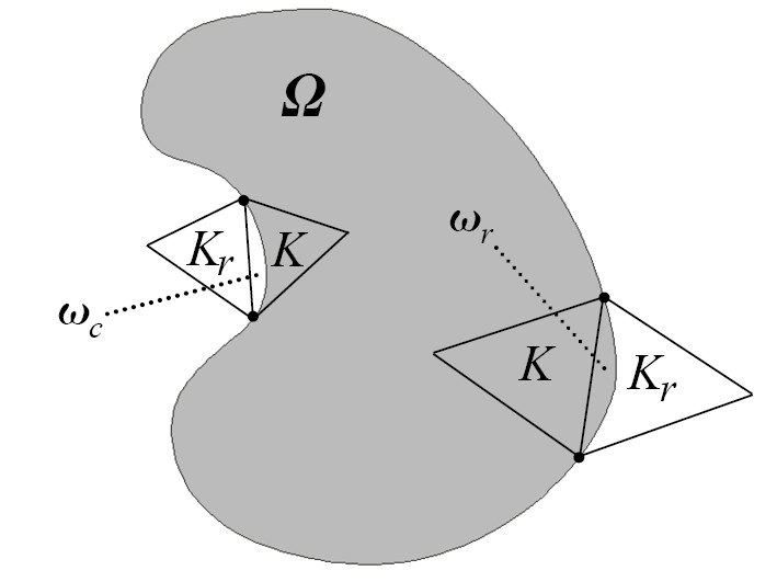
Figure 1. Triangulation of a curved domain.

Here we report on the simple approach of [19]. The idea is to cover $\Omega$ by additional control volumes and to estimate the integral error. To simplify the presentation, let $\Omega\subset{\mathbb{R}}^{2}$ and let ${\mathcal{T}}$ be a sufficiently fine triangulation of $\Omega$ into triangles. To each cell with two vertices on $\partial\Omega$, we add the reflected triangle to the triangulation such that $\Omega\subset\cup_{K\in{\mathcal{T}}^{*}}K$, where ${\mathcal{T}}^{*}$ consists of all cells $K\in{\mathcal{T}}$ and the associated reflected cells $K_{r}$ with nonempty intersection with $\Omega$; see Figure 1. Denoting by $\omega_{r}=K_{r}\cap\Omega$ if $K_{r}\cap\Omega\neq\emptyset$ and $\omega_{c}=K\setminus\Omega$ if $K_{r}\cap\Omega=\emptyset$, the domain splits into

$$\Omega=\Omega_{h}\cup\Omega_{r}\setminus\Omega_{c}:=\bigg{(}\bigcup_{K\in{\mathcal{T}}}K\bigg{)}\cup\bigg{(}\bigcup_{\omega_{r}}\omega_{r}\bigg{)}\setminus\bigg{(}\bigcup_{\omega_{c}}\omega_{c}\bigg{)}.$$

We can perform the numerical analysis on $V_{{\mathcal{T}}^{*}}$ as in Sections 3 and 4. For the convergence of the scheme, we need to show that the difference of the integrals over $\Omega_{h}$ and $\Omega$ vanishes when $\eta_{m}\to 0$. The difference consists of two contributions: the integral over $\Omega_{r}$ and the integral over $\Omega_{c}$. We illustrate the convergence for the integral

$$\bigg{|}\int_{\Omega_{r}}u_{m,i,\sigma}\nabla^{m}(B\widehat{u}_{m})_{i}\cdot\nabla\psi\mathrm{d}x\bigg{|}\leq C\sum_{\omega_{r}}\mathfrak{m}(\omega_{r})\|u_{m,i,\sigma}\|_{0,\infty,\omega_{r}}\|\nabla^{m}(B\widehat{u}_{m})_{i}\|_{0,\infty,\omega_{r}},$$

where $\psi$ is a smooth test function. By the inverse inequality [13, Section 21.1]

$$\|v\|_{0,\infty,\omega_{r}}\leq\|v\|_{0,\infty,K_{r}}\leq C(\Delta x)^{-d/2}\|v\|_{0,2,K_{r}},$$

the bound $\mathfrak{m}(\omega_{r})\leq C(\Delta x)^{d+1}$ (which is valid under certain regularity conditions on the mesh), and the Cauchy–Schwarz inequality, we have

$$\bigg{|}\int_{\Omega_{r}}u_{m,i,\sigma}\nabla^{m}(B\widehat{u}_{m})_{i}\cdot\nabla\psi\mathrm{d}x\bigg{|} \leq C\Delta x\bigg{(}\sum_{K_{r}}\|u_{m,i,\sigma}\|_{0,2,K_{r}}^{2}\bigg{)}^{1/2}\bigg{(}\sum_{K_{r}}\|\nabla^{m}(B\widehat{u}_{m})_{i}\|_{0,2,K_{r}}^{2}\bigg{)}^{1/2}$$

$$\leq C\Delta x\to 0\quad\mbox{as }\eta\to 0,$$

taking into account the uniform bounds from (25) and (26). In a similar way, the integral over $\Omega_{c}$ tends to zero as $\eta\to 0$. ∎

5. Stability

In this section, we prove Theorem 7. Let $\mu$ be a dissipative measure-valued solution and let $v\in C^{1}(\overline{\Omega}_{T})$ be a positive solution of (4), (2). We introduce the relative Shannon and Rao entropies by, respectively,

$$H_{S}^{\rm mv}(u(t)|v(t)) =\sum_{i=1}^{n}\int_{\Omega}\big{(}\langle\mu_{x,t},\mathfrak{h}(s_{i})\rangle-\mathfrak{h}(v_{i}(x,t))-\mathfrak{h}^{\prime}(v_{i}(x,t))\cdot(u_{i}-v_{i})(x,t)\big{)}\mathrm{d}x,$$

$$=\int_{\Omega}\sum_{i=1}^{n}\big{(}\langle\mu_{x,t},s_{i}\log s_{i}\rangle-u_{i}\log v_{i}-(u_{i}-v_{i})\big{)}\mathrm{d}x\geq 0,$$

$$H_{R}(u(t)|v(t)) =\frac{1}{2}\int_{\Omega}|B^{1/2}(u-v)(x,t)|^{2}\mathrm{d}x\geq 0,$$

where $\mathfrak{h}(z)=z(\log z-1)+1$ for $z\geq 0$. We further define the usual relative Shannon entropy $H_{S}(u|v)=\int_{\Omega}\sum_{i=1}^{n}\big{(}u_{i}\log u_{i}-u_{i}\log v_{i}-(u_{i}-v_{i})\big{)}\mathrm{d}x.$ Furthermore, we set

$$H_{\rm rel}^{\rm mv}(u|v)=H_{S}^{\rm mv}(u|v)+H_{R}(u|v),$$

$$H_{\rm rel}(u|v)=H_{S}(u|v)+H_{R}(u|v).$$

We first compute the relative entropy inequalities.

Lemma 15 (Relative entropy inequalities).

Suppose that $\Omega$ has a Lipschitz boundary. Let $\mu$ be a dissipative measure-valued solution, $u:=\langle\mu,s\rangle$, and let $v\in C^{1}(\overline{\Omega}_{T})$ be a positive solution to (4), (2) for $t\in(0,T)$ (in the weak sense). Then, for a.e. $t\in(0,T)$,

(43) $$H_{S}^{\rm mv}(u(t)|v(t))+\int_{0}^{t}\int_{\Omega}\big{\langle}\mu_{x,\tau},|B^{1/2}(p-\nabla v)|^{2}\big{\rangle}\mathrm{d}x\mathrm{d}\tau$$

$$\phantom{x}{}+\int_{0}^{t}\int_{\Omega}\bigg{\langle}\mu_{x,\tau},\sum_{i=1}^{n}(v_{i}-s_{i})\nabla\log v_{i}\cdot(B(p-\nabla v))_{i}\bigg{\rangle}\mathrm{d}x\mathrm{d}\tau\leq H_{S}(u^{\rm in}|v(0)),$$

(44) $$H_{R}(u(t)|v(t))+\int_{0}^{t}\int_{\Omega}\sum_{i=1}^{n}\langle\mu_{x,\tau},s_{i}|(B(p-\nabla v))_{i}|^{2}\rangle\mathrm{d}x\mathrm{d}\tau$$

$$\phantom{x}{}+\int_{0}^{t}\int_{\Omega}\bigg{\langle}\mu_{x,\tau},\sum_{i=1}^{n}(s_{i}-v_{i})\nabla(Bv)_{i}\cdot(B(p-\nabla v))_{i}\bigg{\rangle}\mathrm{d}x\mathrm{d}\tau\leq H_{R}(u^{\rm in}|v(0)).$$

Proof.

It follows from (12) that for all $i=1,\ldots,n$ and $\phi\in L^{2}(0,T;W^{1,4}(\Omega))$

(45) $$\int_{0}^{T}(\partial_{t}u_{i},\phi)_{W^{1,4}(\Omega)^{*}}\mathrm{d}t=-\int_{0}^{T}\int_{\Omega}\langle\mu_{x,t},s_{i}(Bp)_{i}\rangle\cdot\nabla\phi\mathrm{d}x\mathrm{d}t,$$

where $(\cdot,\cdot)_{W^{1,4}(\Omega)^{*}}$ denotes the duality pairing between $W^{1,4}(\Omega)^{*}$ and $W^{1,4}(\Omega)$.

Re Shannon: The solution property and positivity of $v$ imply that for every $\psi\in C^{1}(\overline{\Omega}_{T};{\mathbb{R}}^{n})$,

$$-\sum_{i=1}^{n}\int_{\Omega}(\partial_{t}\log v_{i})\psi_{i}\mathrm{d}x =\int_{\Omega}\sum_{i=1}^{n}v_{i}\nabla(Bv)_{i}\cdot\nabla\bigg{(}\frac{\psi_{i}}{v_{i}}\bigg{)}\mathrm{d}x$$

$$=\int_{\Omega}\nabla v:\nabla(B\widehat{\psi})\mathrm{d}x-\sum_{i=1}^{n}\int_{\Omega}\nabla(Bv)_{i}\cdot(\nabla\log v_{i})\psi_{i}\mathrm{d}x.$$

Let $t\in(0,T)$ be arbitrary. An integration over $\tau\in(0,t)$ and an approximation argument imply that for all $\psi\in L^{2}(\Omega_{T};{\mathbb{R}}^{n})$ with $\nabla B\widehat{\psi}\in L^{2}(\Omega_{T})$,

$$-\sum_{i=1}^{n}\int_{0}^{t}\int_{\Omega}(\partial_{t}\log v_{i})\psi_{i}\mathrm{d}x\mathrm{d}\tau =\int_{0}^{t}\int_{\Omega}\nabla v:\nabla B\widehat{\psi}\mathrm{d}x\mathrm{d}\tau$$

$$\phantom{xx}{}-\sum_{i=1}^{n}\int_{0}^{t}\int_{\Omega}\nabla(Bv)_{i}\cdot(\nabla\log v_{i})\,\psi_{i}\mathrm{d}x\mathrm{d}\tau.$$

The choice $\psi=u=\langle\mu,s\rangle$ and the property $\nabla B\widehat{u}=B\langle\mu,p\rangle=\langle\mu,Bp\rangle$ lead to

$$-\sum_{i=1}^{n} \int_{0}^{t}\int_{\Omega}(\partial_{t}\log v_{i})u_{i}\mathrm{d}x\mathrm{d}\tau=$$

$$=\int_{0}^{t}\int_{\Omega}\nabla v:\nabla B\widehat{u}\mathrm{d}x\mathrm{d}\tau-\sum_{i=1}^{n}\int_{0}^{t}\int_{\Omega}\nabla(Bv)_{i}\cdot(\nabla\log v_{i})u_{i}\mathrm{d}x\mathrm{d}\tau$$

$$=\int_{0}^{t}\int_{\Omega}\langle\mu_{x,\tau},B^{1/2}\nabla v:B^{1/2}p\rangle\mathrm{d}x\mathrm{d}\tau-\sum_{i=1}^{n}\int_{0}^{t}\int_{\Omega}\langle\mu_{x,\tau},s_{i}\nabla\log v_{i}\cdot\nabla(Bv)_{i}\rangle\mathrm{d}x\mathrm{d}\tau.$$

Next, we use $\phi_{i}=1_{[0,t]}\log v_{i}$ as a test function in the weak formulation (45), multiply by $-1$, and sum over $i=1,\dots,n$:

$$-\sum_{i=1}^{n}\int_{0}^{t}(\partial_{t}u_{i},\log v_{i})_{W^{1,4}(\Omega)^{*}}\mathrm{d}\tau=\sum_{i=1}^{n}\int_{0}^{t}\int_{\Omega}\langle\mu_{x,\tau},s_{i}(Bp)_{i}\rangle\cdot\nabla\log v_{i}\mathrm{d}x\mathrm{d}\tau.$$

We add the previous two equations:

$$-\int_{0}^{t}\frac{\mathrm{d}}{\mathrm{d}t}\int_{\Omega}\sum_{i=1}^{n}(\log v_{i})u_{i}\mathrm{d}x\mathrm{d}\tau =\int_{0}^{t}\int_{\Omega}\langle\mu_{x,\tau},B^{1/2}\nabla v:B^{1/2}p\rangle\mathrm{d}x\mathrm{d}\tau$$

$$\phantom{xx}{}+\int_{0}^{t}\int_{\Omega}\langle\mu_{x,\tau},\sum_{i=1}^{n}s_{i}\nabla\log v_{i}\cdot(B(p-\nabla v))_{i}\rangle\mathrm{d}x\mathrm{d}\tau.$$

Combined with the identity

$$\int_{0}^{t}\int_{\Omega}\langle\mu_{x,\tau},B^{1/2}\nabla v:B^{1/2}p\rangle\mathrm{d}x\mathrm{d}\tau -\int_{0}^{t}\int_{\Omega}\langle\mu_{x,\tau},|B^{1/2}\nabla v|^{2}\rangle\mathrm{d}x\mathrm{d}\tau$$

$$-\int_{0}^{t}\int_{\Omega}\bigg{\langle}\mu_{x,\tau},\sum_{i=1}^{n}v_{i}\nabla\log v_{i}\cdot(B(p-\nabla v))_{i}\bigg{\rangle}\mathrm{d}x\mathrm{d}\tau=0,$$

the Shannon entropy inequality (10), and mass conservation $(\mathrm{d}/\mathrm{d}t)\int_{\Omega}v_{i}\,\mathrm{d}x=0$, this gives (43).

Re Rao: Since $v_{i}\nabla(Bv)_{i}\in L^{2}(\Omega_{T})$, we can test the equation for $v$ with $1_{[0,t]}\,B(v-u)\in L^{2}(0,T;H^{1}(\Omega))$. This yields

$$\int_{0}^{t}\int_{\Omega}\partial_{t}v^{T}B(v-u)\mathrm{d}x\mathrm{d}\tau=-\int_{0}^{t}\int_{\Omega}\sum_{i=1}^{n}v_{i}\nabla(Bv)_{i}\cdot\nabla(B(v-u))_{i}\mathrm{d}x\mathrm{d}\tau.$$

Next, we choose $\phi=1_{[0,t]}(Bv)_{i}$ in equation (45) for $u$ and sum over $i=1,\dots,n$:

$$-\int_{0}^{t}(\partial_{t}u,Bv)_{W^{1,4}(\Omega)^{*}}\mathrm{d}\tau=\int_{0}^{t}\int_{\Omega}\sum_{i=1}^{n}\langle\mu_{x,\tau},s_{i}(Bp)_{i}\rangle\cdot(B\nabla v)_{i}\mathrm{d}x\mathrm{d}\tau.$$

Adding to these identities the Rao entropy inequality (11) and rearranging terms gives

$$\frac{1}{2}\int_{0}^{t}\frac{\mathrm{d}}{\mathrm{d}t}\int_{\Omega}(u-v)^{T}B(u-v)\mathrm{d}x\mathrm{d}\tau \leq-\int_{0}^{t}\int_{\Omega}\sum_{i=1}^{n}\langle\mu_{x,\tau},s_{i}|(B(p-\nabla v))_{i}|^{2}\rangle\mathrm{d}x\mathrm{d}\tau$$

$${}-\int_{0}^{t}\int_{\Omega}\sum_{i=1}^{n}\langle\mu_{x,\tau},(s_{i}-v_{i})(B\nabla v)_{i}\cdot(B(p-\nabla v))_{i}\mathrm{d}x\mathrm{d}\tau,$$

which implies (44), concluding the proof. ∎

We proceed with the proof of Theorem 7. To this end, we estimate the last integrals on the left-hand sides of (43) and (44). We infer from Young’s inequality that

(46) $$\bigg{|}\sum_{i=1}^{n} (v_{i}-s_{i})\nabla\log v_{i}\cdot(B(p-\nabla v))_{i}\bigg{|}$$

$$\leq\frac{1}{4}|B^{1/2}(p-\nabla v)|^{2}+C\sum_{i=1}^{n}|\nabla\log v_{i}|^{2}(s_{i}-v_{i})^{2}$$

$$\leq\frac{1}{4}|B^{1/2}(p-\nabla v)|^{2}+C|s-v|^{2},$$

(47) $$\bigg{|}\sum_{i=1}^{n} (s_{i}-v_{i})\nabla(Bv)_{i}\cdot(B(p-\nabla v))_{i}\bigg{|}$$

$$\leq\frac{1}{4}|B^{1/2}(p-\nabla v)|^{2}+C\sum_{i=1}^{n}|\nabla(Bv)_{i}|^{2}(s_{i}-v_{i})^{2}$$

$$\leq\frac{1}{4}|B^{1/2}(p-\nabla v)|^{2}+C|s-v|^{2},$$

where $C>0$ depends on the $L^{\infty}(\Omega_{T})$ norms of $|\nabla\log v_{i}|$ and $\nabla(Bv)_{i}$. Thus, adding the relative entropy inequalities (43) and (44), the first terms on the right-hand sides of (46) and (47) can be absorbed by the left-hand side of (43) such that

(48) $$\begin{aligned} H_{\rm rel}^{\rm mv}(u(t)|v(&t))+\int_{0}^{t}\int_{\Omega}\bigg{\langle}\mu_{x,\tau},\frac{1}{2}|B^{1/2}(p-\nabla v)|^{2}\bigg{\rangle}\mathrm{d}x\mathrm{d}\tau\\ &\leq C\int_{0}^{t}\int_{\Omega}\langle\mu_{x,\tau},|s-v|^{2}\rangle\mathrm{d}x\mathrm{d}\tau+H_{\rm rel}(u^{\rm in}|v(0)).\end{aligned}$$

The coercivity estimate from Lemma 17 in Appendix A implies that

$$\int_{\Omega}\langle\mu_{x,t},|s-v(x,t)|^{2}\rangle\mathrm{d}x\leq CH_{\rm rel}^{\rm mv}(u(t)|v(t)).$$

We insert this bound into (48) and invoke Gronwall’s inequality to deduce that

$$H_{\rm rel}^{\rm mv}(u(t)|v(t)) +\int_{0}^{t}\int_{\Omega}\bigg{\langle}\mu_{x,\tau},\frac{1}{2}|B^{1/2}(p-\nabla\widehat{v}(x,\tau))|^{2}\bigg{\rangle}\mathrm{d}x\mathrm{d}\tau\leq{\rm e}^{Ct}H_{\rm rel}(u^{\rm in}|v(0))=0,$$

where the last equality follows from $v(0)=u^{\rm in}$. Hence, $\mu_{x,t}=\delta_{v(x,t)}\otimes\delta_{\nabla\widehat{v}(x,t)}$ for a.e. $(x,t)\in\Omega\times(0,T)$, which finishes the proof of Theorem 7.

6. Long-time asymptotics

In this section, we prove Theorem 9. First, we verify that $\mathfrak{S}_{\mathsf{m}}\subset L^{\infty}(\Omega)$. Indeed, if $v\in\mathfrak{S}_{\mathsf{m}}$, the vector $Bv$ is constant and $\int_{\Omega}Bv\mathrm{d}x=B\mathsf{m}$, which implies that $Bv=(B\mathsf{m})/|\Omega|$. Since the entries of $B$ and the components of $v$ are nonnegative, $v_{i}\leq(B\mathsf{m})_{i}/(b_{ii}|\Omega|)$ for all $i=1,\ldots,n$. This proves the claim.

The entropy inequalities (10)–(11) and the bound $|\langle\mu,B^{1/2}p\rangle|^{2}\leq\langle\mu,|B^{1/2}p|^{2}\rangle$, which follows from Jensen’s inequality, show that

$$\int_{0}^{\infty}\|\nabla(B^{1/2}u)\|_{L^{2}(\Omega)}^{2}\mathrm{d}t<\infty,\quad\sup_{0<t<\infty}\|u(t)\|_{L^{2}(\Omega)}<\infty.$$

Thus, there exists a sequence $(t_{k})\subset(0,\infty)$ with $t_{k}\to\infty$ such that $u(t_{k})\rightharpoonup u^{*}$ weakly in $L^{2}(\Omega)$ and $B^{1/2}u(t_{k})\to B^{1/2}u^{*}$ strongly in $L^{2}(\Omega)$ as $k\to\infty$. Since $\int_{\Omega}u(t_{k})\mathrm{d}x=\mathsf{m}$ and the sequence $(\nabla(B^{1/2}u(t_{k})))$ converges to zero in the $L^{2}(\Omega)$ norm, we find that $\int_{\Omega}u^{*}\mathrm{d}x=\mathsf{m}$ and $\nabla(B^{1/2}u^{*})=0$. This implies that $u^{*}\in\mathfrak{S}_{\mathsf{m}}$. Moreover, we deduce from the strong convergence that

$$\lim_{k\to\infty}H_{R}(u(t_{k})|u^{*})=\frac{1}{2}\lim_{k\to\infty}\|B^{1/2}(u(t_{k})-u^{*})\|_{L^{2}(\Omega)}^{2}=0.$$

We assert that $t\mapsto H_{R}(u(t)|u^{*})$ is nonincreasing for a.e. $t>0$. Indeed, we know from Section 4.3 that $t\mapsto H_{R}(u(t))$ is nonincreasing. Furthermore, since $\int_{\Omega}u(t)\mathrm{d}x=\int_{\Omega}u^{*}\mathrm{d}x$ and $Bu^{*}$ is a constant vector, we have $\int_{\Omega}u(t)^{T}Bu^{*}\mathrm{d}x=\int_{\Omega}u(s)^{T}Bu^{*}\mathrm{d}x$ for $t\geq s$. Hence, for $t\geq s$,

$$H_{R}(u(t)|u^{*}) =H_{R}(u(t))+H_{R}(u^{*})-\int_{\Omega}u(t)^{T}Bu^{*}\mathrm{d}x$$

$$\leq H_{R}(u(s))+H_{R}(u^{*})-\int_{\Omega}u(s)^{T}Bu^{*}\mathrm{d}x=H_{R}(u(s)|u^{*}),$$

proving the claim.

We conclude that $H_{R}(u(t)|u^{*})\leq H_{R}(u(t_{k})|u^{*})\to 0$ for $t\geq t_{k}\to\infty$. It follows from the positive definiteness of $B^{1/2}$ on $L^{\perp}$ that

$$\|\widehat{u}(t)-\widehat{u}^{*}\|_{L^{2}(\Omega)}\leq C\|B^{1/2}(\widehat{u}(t)-\widehat{u}^{*})\|_{L^{2}(\Omega)}\leq 2H_{R}(u(t)|u^{*})\to 0$$

as $t\to\infty$. This finishes the proof of Theorem 9.

Appendix A Auxiliary results

Let the matrix $B=(b_{ij})\in{\mathbb{R}}^{n\times n}$ be symmetric positive semidefinite. Then the square root of $B^{1/2}$ exists and $z^{T}Bz=|B^{1/2}z|^{2}$ for $z\in{\mathbb{R}}^{n}$. Let $P_{L}$ and $P_{L^{\perp}}$ be the projection matrices onto $L=\operatorname{ker}B=\operatorname{ker}B^{1/2}\neq\{0\}$ and $L^{\perp}=\operatorname{ran}B$, respectively.

Lemma 16.

Let $\lambda>0$ be the smallest positive eigenvalue of $B^{1/2}$. Then

$$|P_{L^{\perp}}z|\leq\lambda^{-1}|B^{1/2}z|\quad\mbox{for }z\in{\mathbb{R}}^{n}.$$

Proof.

Let $z\in{\mathbb{R}}^{n}$ and $\widehat{z}=P_{L^{\perp}}z$. By definition of $\lambda$, $|B^{1/2}\widehat{z}|^{2}\geq\lambda|\widehat{z}|^{2}$. Then the conclusion follows from $B^{1/2}\widehat{z}=B^{1/2}z-B^{1/2}P_{L}z=B^{1/2}z$. ∎

We introduce the relative entropy densities

$$h_{S}(u|v) =\sum_{i=1}^{n}\big{(}\mathfrak{h}(u_{i})-\mathfrak{h}(v_{i})-\mathfrak{h}^{\prime}(v_{i})(u_{i}-v_{i})=\sum_{i=1}^{n}\bigg{(}u_{i}\log\frac{u_{i}}{v_{i}}-(u_{i}-v_{i})\bigg{)},$$

$$h_{R}(u|v) =\frac{1}{2}(u-v)^{T}B(u-v)=\frac{1}{2}|B^{1/2}(u-v)|^{2},\quad u,v\in[0,\infty)^{n},$$

where $\mathfrak{h}(z)=z(\log z-1)+1$. We denote by $\|A\|_{2}$ the norm of $A$ induced by the Euclidean norm $|\cdot|$ in ${\mathbb{R}}^{n}$.

Lemma 17 (Coercivity).

Let $a_{0}=\frac{1}{2}\min_{i\in\{1,\ldots,n\}}b_{ii}>0$, $a_{1}=\|B\|_{2}$, and let $K\geq 1$. Then there exists a constant $c_{*}>0$, only depending on $a_{0}$, $a_{1}/a_{0}$, and $M$, such that for all $u$, $v\in{\mathbb{R}}_{\geq}^{n}$ with $0<|v|\leq M$,

$$h_{S}(u|v)+h_{R}(u|v)\geq c_{*}|u-v|^{2}.$$

Proof.

By assumption, we have $\frac{1}{2}u^{T}Bu\geq\frac{1}{2}\sum_{i=1}^{n}b_{ii}u_{i}^{2}\geq a_{0}|u|^{2}$ for all $u\in{\mathbb{R}}_{\geq}^{n}$. If $(a_{0}/2)|u|\geq a_{1}|v|$ then

$$h_{R}(u|v) =\frac{1}{2}u^{T}Bv-v^{T}Bu+\frac{1}{2}v^{T}Bv\geq a_{0}|u|^{2}-a_{1}|u||v|+a_{0}|v|^{2}$$

$$\geq a_{0}|u|^{2}-\frac{a_{0}}{2}|u|^{2}+a_{0}|v|^{2}=\frac{a_{0}}{2}|u|^{2}+a_{0}|v|^{2}\geq\frac{a_{0}}{3}|u-v|^{2}.$$

Next let $(a_{0}/2)|u|<a_{1}|v|$. We find for $f(z)=z\log z$ that

$$u_{i}\log \frac{u_{i}}{v_{i}}-(u_{i}-v_{i})=f(u_{i})-f(v_{i})-f^{\prime}(v_{i})(u_{i}-v_{i})$$

$$=(u_{i}-v_{i})\int_{0}^{1}\big{(}f^{\prime}(s(u_{i}-v_{i})+v_{i})-f^{\prime}(v_{i})\big{)}\big{|}_{s=0}^{\theta}\mathrm{d}\theta$$

$$=(u_{i}-v_{i})^{2}\int_{0}^{1}\int_{0}^{\theta}f^{\prime\prime}(s(u_{i}-v_{i})+v_{i})\mathrm{d}s\mathrm{d}\theta.$$

Then we infer from $|u_{i}/v_{i}|<2a_{1}/a_{0}$ that

$$f^{\prime\prime}(s(u_{i}-v_{i})+v_{i})=\frac{1}{v_{i}(s(u_{i}/v_{i}-1)+1)}>\frac{1}{M(s(2a_{1}/a_{0}-1)+1)}$$

and consequently,

$$u_{i}\log\frac{u_{i}}{v_{i}}-(u_{i}-v_{i})\geq\frac{(u_{i}-v_{i})^{2}}{M}\int_{0}^{1}\int_{0}^{\theta}\frac{\mathrm{d}s\mathrm{d}\theta}{s(2a_{1}/a_{0}-1)+1},$$

which shows that $h_{S}(u|v)\geq c_{1}|u-v|^{2}$, where

$$c_{1}=\frac{1}{M}\min_{i=1,\ldots,n}\int_{0}^{1}\int_{0}^{\theta}\frac{\mathrm{d}s\mathrm{d}\theta}{s(2a_{1}/a_{0}-1)+1}.$$

Putting these estimates together and observing that $h_{S}(u|v)\geq 0$, $h_{R}(u|v)\geq 0$, we conclude the proof with $c_{*}=\min\{a_{0}/3,c_{1}\}$. ∎

References

• [1] H. Amann. Nonhomogeneous linear and quasilinear elliptic and parabolic boundary value problems. In: H. J. Schmeisser and H. Triebel (eds.), Funct. Spaces Diff. Oper. Nonlin. Anal., pp. 9–126. Teubner, Wiesbaden, 1993.
• [2] M. Bertsch, M. Gurtin, D. Hilhorst, and L. Peletier. On interacting populations that disperse to avoid crowding: preservation of segregation. J. Math. Biol. 23 (1985), 1–13.
• [3] M. Bertsch, D. Hilhorst, H. Izuhara, and M. Mumura. A nonlinear parabolic-hyperbolic system for contact inhibition of cell-growth. Diff. Eqs. Appl. 4 (2012), 137–157.
• [4] D. Bothe. On the Maxwell–Stefan equations to multicomponent diffusion. In: Progress in Nonlinear Differential Equations and their Applications, pp. 81–93. Springer, Basel, 2011.
• [5] Y. Brenier, C. De Lellis, L. Székelyhidi. Weak–strong uniqueness for measure-valued solutions. Commun. Math. Phys. 305 (2011), 351–361.
• [6] M. Burger, J. A. Carrillo, J.-F. Pietschmann, and M. Schmidtchen. Segregation effects and gap formation in cross-diffusion models. Interfaces Free Bound. 22 (2020), 175–203.
• [7] J. A. Cañizo, J. A. Carrillo, P. Laurençot, and J. Rosado. The Fokker–Planck equation for bosons in 2D: well-posedness and asymptotic behavior. Nonlin. Anal. 137 (2016), 291–305.
• [8] C. Chainais-Hillairet, J.-G. Liu, and Y.-J. Peng. Finite volume scheme for multi-dimensional drift-diffusion equations and convergence analysis. ESAIM Math. Model. Numer. Anal. 37 (2003), 319–338.
• [9] L. Chen, E. Daus, and A. Jüngel. Rigorous mean-field limit and cross diffusion. Z. Angew. Math. Phys. 70 (2019), no. 122, 21 pages.
• [10] C. Christoforou and A. Tzavaras. Relative entropy for hyperbolic–parabolic systems and application to the constitutive theory of thermoviscoelasticity. Arch. Ration. Mech. Anal. 229 (2018), 1–52.
• [11] S. Demoulini, D. Stuart, and A. Tzavaras. Weak–strong uniqueness of dissipative measure-valued solutions for polyconvex elastodynamics. Arch. Ration. Mech. Anal. 205 (2012), 927–961.
• [12] K. Deimling. Nonlinear Functional Analysis. Springer, Berlin, 1985.
• [13] A. Ern and J.-L. Guermond. Finite Elements I: Approximation and Interpolation. Springer, Cham, 2021.
• [14] J. Escher, A.-V. Matioc, and B.-V. Matioc. Modelling and analysis of the Muskat problem for thin fluid layers. J. Math. Fluid Mech. 14 (2012), 267–277.
• [15] M. Di Francesco, A. Esposito, and S. Fagioli. Nonlinear degenerate cross-diffusion systems with nonlocal interaction. Nonlin. Anal. 169 (2018), 94–117.
• [16] R. DiPerna. Measure-valued solutions to conservation laws. Arch. Ration. Mech. Anal. 88 (1985), 223–270.
• [17] P.-E. Druet, K. Hopf, and A. Jüngel.. Hyperbolic–parabolic normal form and local classical solutions for cross-diffusion systems with incomplete diffusion. Submitted for publication, 2022. arXiv:2210.17244.
• [18] P.-E. Druet and A. Jüngel. Analysis of cross-diffusion systems for fluid mixtures driven by a pressure gradient. SIAM J. Math. Anal. 52 (2020), 2179–2197.
• [19] C. Elliott and V. Janosvsky. An error estimate for a finite-element approximation of an elliptic variational inequality formulation of a Hele–Shaw moving-boundary problem. IMA J. Numer. Anal. 3 (1983), 1–9.
• [20] R. Eymard, T. Gallouët, and R. Herbin. Finite volume methods. In: P. G. Ciarlet and J.-L. Lions (eds.). Handbook of Numerical Analysis 7 (2000), 713–1018.
• [21] E. Feireisl, P. Gwiazda, A. Świerczewska-Gwiazda, and E. Wiedemann. Dissipative measure-valued solutions to the compressible Navier–Stokes system. Calc. Var. Partial Diff. Eqs. 55 (2016), no. 141, 20 pages.
• [22] E. Feireisl and M. Lukáčová-Medvid’ová. Convergence of a mixed finite element–finite volume scheme for the isentropic Navier–Stokes system via dissipative measure-valued solutions. Found. Comput. Math. 18 (2018), 703–730.
• [23] E. Feireisl, M. Lukáčová-Medvid’ová, and H. Mizerová. Convergence of finite volume schemes for the Euler equations via dissipative measure-valued solutions. Found. Comput. Math. 20 (2020), 923–966.
• [24] U. Fjordholm, R. and Käppeli, S. Mishra, and E. Tadmor. On the computation of measure-valued solutions. Acta Numerica 25 (2016), 567–679.
• [25] K. Friedrichs and P. Lax. Systems of conservation equations with a convex extension. Proc. Nat. Acad. Sci. USA 68 (1971), 1686–1688.
• [26] T. Gallouët and J.-C. Latché. Compactness of discrete approximate solutions to parabolic PDEs – Application to a turbulence model. Commun. Pure Appl. Anal. 11 (2012), 2371–2391.
• [27] P. Gwiazda, B. Perthame, and A. Świerczewska-Gwiazda. A two-species hyperbolic–parabolic model of tissue growth. Commun. Partial Diff. Eqs. 44 (2019), 1605–1618.
• [28] P. Gwiazda, A. Świerczewska-Gwiazda, and E. Wiedemann. Weak–strong uniqueness for measure-valued solutions of some compressible fluid models. Nonlinearity 28 (2015), 3873–3890.
• [29] K. Hopf. Singularities in $L^{1}$-supercritical Fokker–Planck equations: A qualitative analysis. arXiv:2107.08531. (Accepted for publication in Ann. Inst. H. Poincaré C, Anal. Non Lin.)
• [30] M. Jacobs. Non-mixing solutions to the multispecies porous media equation. Submitted for publication, 2022. arXiv:2208.01792.
• [31] A. Jüngel. Entropy Methods for Diffusive Partial Differential Equations. Springer Briefs Math., Springer, 2016.
• [32] A. Jüngel, S. Portisch, and A. Zurek. Nonlocal cross-diffusion systems for multi-species populations and networks. Nonlin. Anal. 219 (2022), 112800, 26 pages.
• [33] A. Jüngel and I. Stelzer. Existence analysis of Maxwell–Stefan systems for multicomponent mixtures. SIAM J. Math. Anal. 45 (2013), 2421–2440.
• [34] A. Jüngel and A. Zurek. A finite-volume scheme for a cross-diffusion model arising from interacting many-particle population systems. In: R. Klöfkorn, E. Keilegavlen, F. Radu, and J. Fuhrmann (eds.), Finite Volumes for Complex Applications IX, pp. 223–231. Springer, Cham, 2020.
• [35] A. Jüngel and A. Zurek. A convergent structure-preserving finite-volume scheme for the Shigesada–Kawasaki–Teramoto population system. SIAM J. Numer. Anal. 59 (2021), 2286–2309.
• [36] S. Kawashima and Y. Shizuta. On the normal form of the symmetric hyperbolic–parabolic systems associated with the conservation laws. Tohoku Math. J. 40 (1988), 449–464.
• [37] P. Laurençot and B. Matioc. Weak–strong uniqueness for a class of degenerate parabolic cross-diffusion systems. Arch. Math. (Brno) 59 (2023), 201–213.
• [38] P.-L. Lions. Mathematical topics in fluid dynamics. Vol. 1: Incompressible models. Oxford Science Publication, Oxford, 1996.
• [39] T. Lorenzi, A. Lorz, and B. Perthame. On interfaces between cell populations with different mobilities. Kinet. Relat. Models 10 (2017), 299–311.
• [40] F. Nabet. Convergence of a finite-volume scheme for the Cahn–Hilliard equation with dynamic boundary conditions. IMA J. Numer. Anal. 36 (2016), 1898–1942.
• [41] A. Oulhaj. Numerical analysis of a finite volume scheme for a seawater intrusion model with cross-diffusion in an unconfined aquifer. Numer. Meth. Partial Diff. Eqs. 34 (2018), 857–880.
• [42] P. Pedregal. Parametrized Measures and Variational Principles. Birkhäuser, Basel, 1997.
• [43] C. Rao. Diversity and dissimilarity coefficients: a unified approach. Theor. Popul. Biol. 21 (1982), 24–43.
• [44] L. Tartar. Compensated compactness and applications to partial differential equations. In: R. Knops (ed.), Nonlinear Analysis and Mechanics: Heriot–Watt Symposium, Res. Notes Math. 39, pp. 136–212. Pitman, Boston, 1979.