Petermann factors and phase rigidities near exceptional points
Abstract
The Petermann factor and the phase rigidity are convenient measures for various aspects of open quantum and wave systems, such as the sensitivity of energy eigenvalues to perturbations or the magnitude of quantum excess noise in lasers. We discuss the behavior of these two important quantities near non-Hermitian degeneracies, so-called exceptional points. For small generic perturbations, we derive analytically explicit formulas which reveal a relation to the spectral response strength of the exceptional point. These formulas shed light on the possibilities for enhanced sensing in passive systems. The predictions of the general theory are successfully compared to analytical solutions of a toy model. Moreover, it is demonstrated that the connection between the Petermann factor and the spectral response strength provides the basis for an efficient numerical scheme to calculate the latter. Our theory is also important in the presence of the unavoidable imperfections in the fabrication of exceptional points as it allows to determine of what is left of the sensitivity for such imperfect exceptional points studied in experiments.
I Introduction
Non-Hermitian effective Hamiltonians [1, 2] describing the dynamics of open quantum and wave systems have attracted considerable interest in recent years, in particular in the context of non-Hermitian photonics [3, 4]. One obvious consequence of the non-Hermiticity (or nonself-adjointness) of the Hamiltonian is that the energy eigenvalues can be complex-valued. The imaginary part has the clear physical interpretation as a decay or growth rate. Another consequence is that if, additionally, the Hamiltonian is nonnormal, , then one has to distinguish right eigenstates from the corresponding left eigenstates ; the quantum number labels the states uniquely. The difference of right and left eigenstates is an indicator of the strength of “non-Hermitian effects”, or better said, “nonnormal effects”. This can be made more precise in terms of the Petermann factor of a given pair of eigenstates
| (1) |
with the conventional inner product in Hilbert space. There exists a lower bound which follows from the Cauchy-Schwarz inequality . The Petermann factor has been introduced to quantify the linewidth broadening resulting from quantum excess noise in lasers [5, 6, 7, 8, 9, 10] and laser gyroscopes [11]. It is therefore also called excess-noise factor or excess-spontaneous emission factor. Moreover, the Petermann factor measures the enhanced response of the corresponding eigenstate to perturbations [12], which is important for non-Hermitian topological sensors [13] and appears also in the context of the non-Hermitian skin effect, see, e.g., Ref. [14]. In the mathematical literature on nonnormal eigenvalue problems, the enhanced response is equivalently discussed in terms of the condition number (square root of the Petermann factor) in the Bauer-Fike theorem [15] or in terms of the pseudospectrum [16]. Even though is defined as a quantity characterizing the individual eigenstate with quantum number it also describes mutual non-orthogonality of eigenstates in two-dimensional Hilbert spaces where the Petermann factors can be written as with normalized eigenstates [17].
Another but equivalent quantity to characterize the difference of right and left eigenstates is the phase rigidity
| (2) |
with . There are other, slightly different, definitions in the literature. Some agree with Eq. (2) provided that the normalization of the individual eigenstates are chosen appropriately [18, 19, 20]. Some other definitions agree only for (complex-) symmetric Hamiltonians and proper normalization [21, 22, 23, 24, 25]. The phase rigidity had been originally invented to quantify the complexness of wavefunctions in systems with partially broken time-reversal symmetry [21]. A related quantity has been used to observe signatures of quantum chaos in open billiard systems [26].
Of particular interest in the field of open systems are exceptional points (EPs) in parameter space [27, 28, 29, 30, 31]. At such an EP of order a variety of interesting phenomena appear. (i) Exactly eigenstates and their corresponding eigenvalues of the Hamiltonian coalesce. (ii) When the Hamiltonian is subjected to a small perturbation of strength then the resulting eigenvalue changes are generically proportional to the th root of [27]. This feature can be exploited for sensing applications [32, 33, 34, 35, 36, 37, 38]. The response of the system at the EP in terms of eigenvalue changes can be quantified by the spectral response strength [39]. (iii) The overlap of each involved eigenstate of the Hamiltonian vanishes [40, 41]. The latter implies that the corresponding Petermann factors [Eq. (1)] diverge to infinity [42, 43] and the phase rigidities [Eq. (2)] vanish [23] whenever an EP is approached. This has been exploited as an indicator for the appearance of an EP [18, 24, 20, 19, 25]. The scaling of the Petermann factors near a second-order EP have been studied numerically in Refs. [44, 45, 46]. For the phase rigidities such numerical studies have been performed for EPs also of higher order [18, 24, 19, 25]. For a generic perturbation with small perturbation strength , a power law with scaling exponent for the phase rigidities is expected [47]. The scaling exponent, and in particular deviations from the expected value, have been used to characterize the EP [18, 24, 20, 19, 25, 44, 46, 45].
In this paper, we present a theory for the Petermann factors and the phase rigidities near an EP of arbitrary order. This theory allows to accurately predict their behavior in this extreme situation. In particular, we determine the coefficient in the power law . We are able to relate this coefficient directly to the spectral response strength of the EP. This relation provides a basis for the calculation of the spectral response strength.
The outline of the paper is as follows. In Sec. II some necessary theoretical concepts are reviewed. The scaling properties of the Petermann factors and the phase rigidities near EPs are derived in Sec. III. Bounds for these quantities are introduced in Sec. IV. The results are briefly compared to the literature in Sec. V. An example and an application are presented in Secs. VI and VII. Section VIII provides a conclusion.
II Preliminaries
This section introduces the theoretical concepts necessary for understanding this paper.
II.1 Jordan vectors
We consider an -Hamiltonian at an EP of order with right eigenstate and eigenvalue . Clearly, a single state cannot span a basis in the -dimensional Hilbert space. A basis can be established by the linearly independent (right) Jordan vectors . We introduce the -matrix
| (3) |
which is nilpotent of index ; hence but . The operator is the identity. With the operator the Jordan chain (see, e.g., Ref. [48]) is defined as
| (4) | |||||
| (5) |
It is important to realize that only is a right eigenstate of the Hamiltonian. Note that Eqs. (4) and (5) do not uniquely determine the Jordan vectors. This can be fixed (up to a complex phase) by requiring [39]
| (6) | |||||
| (7) |
II.2 Spectral response strength
In Ref. [39] the spectral response strength of a system at an EP of order has been determined to be
| (8) |
with the -matrix defined in Eq. (3) and the spectral norm (see, e.g., Ref. [49])
| (9) |
We obey the conventional notation both for the spectral norm of a matrix [in the left-hand side of Eq. (9)] and the 2-norm of a vector [in the right-hand side of Eq. (9)]. The spectral response strength describes the response of the system at the EP to perturbations,
| (10) |
in terms of a factor in the bound of the eigenvalue change
| (11) |
where higher orders in the perturbation strength are ignored. The scaling of with the th root of is a manifestation of the enhanced sensitivity of the system at the EP with respect to perturbations. Inequality (11) is valid for generic perturbations, which means here . In very special situations, parameter variations can correspond to nongeneric perturbations leading to a different scaling behavior. This phenomenon is called anisotropic EP, see, e.g., Ref. [19]. It can happen that symmetries lead to nongeneric perturbations, see Refs. [50, 51]. The presence of a nongeneric perturbation would require to extend the theory presented in Ref. [39] by incorporating the next-order contribution in the Green’s function.
III Petermann factors and phase rigidities near an EP
In this section we derive explicit expressions for the Petermann factors [Eq. (1)] and the phase rigidities [Eq. (2)] valid near a given EP of order .
Let us first specify the definition of right and left eigenstates (see, e.g., Ref. [52]) of the Hamiltonian
| (13) |
There are different possibilities to normalize two of the three inner products , , and . Without loss of generality, we choose the normalization for all . In this case the Petermann factors are
| (14) |
and the phase rigidities
| (15) |
The central quantity to compute is therefore .
We start with the perturbed Hamiltonian (10) and add another perturbation with . For what follows it is crucial that the two perturbations can be combined to . The change in the eigenvalues can be evaluated in first-order non-Hermitian perturbation theory [13]
| (16) |
In the limit we can write
| (17) |
For a generic perturbation the eigenvalue change is with [27]. The -dependence of originates from the primitive th root of unity with . We deduce that
| (18) |
Moreover, in leading order we can approximate by
| (19) |
and therefore with Eqs. (17) and (18)
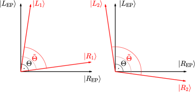
| (20) |
This equation is illustrated in Fig. 1.
To calculate the right-hand side of Eq. (20) we first expand in terms of the Jordan vectors
| (21) |
In conjunction with and for [see the Jordan chain in Eqs. (4) and (5)] we get
| (22) |
In Ref. [53] it has been shown that generically for small perturbations
| (23) |
In the leading order we replace by and back resulting with the help of Eq. (10) in
| (24) | |||||
In combination with Eq. (22) we then get
| (25) |
Next, we take advantage of the relation proven in Appendix A
| (26) |
with Kronecker delta . Together with Eqs. (20) and (21) we obtain
| (27) |
With Eqs. (12), (15), and (25) we get our central result for the phase rigidities
| (28) |
Since the absolute value of the eigenvalue change in the leading order is independent of the quantum number [53] we conclude that the same is true for the phase rigidities. Hence, in the following we speak about the phase rigidity in the vicinity of the EP. Of course, this also applies to the Petermann factor(s) [Eq. (14)]
| (29) |
In contrast to inequality (11), Eqs. (28) and (29) are really equations. Hence, the spectral response strength here does not just describe a bound but an exact relationship.
At first glance, it might be surprising that the Petermann factor and the phase rigidity are related to the spectral response strength and not to the eigenstate response strength defined in Ref. [39]. After all, the Petermann factor and the phase rigidity have been introduced as measures of the eigenstates. But both quantities are also related to spectral properties via the first-order non-Hermitian perturbation theory as visible in Eq. (16).
IV Bounds
We combine Eqs. (28) and (29) with inequality (11) leading to the bounds
| (30) |
and
| (31) |
These inequalities provide easy-to-calculate bounds for the phase rigidity and the Petermann factor provided that the spectral response strength of the EP is known and the size of the perturbation can be calculated or at least estimated.
For passive (no gain) systems Ref. [54] has derived an upper bound for the spectral response strength
| (32) |
Based on this inequality we derive an upper bound for the Petermann factor in Eq. (29)
| (33) |
An analog inequality for the phase rigidity can be easily derived.
The inequality (33) has an important consequence. Assume that we want to utilize our system as a sensor but in contrast to a conventional EP-based sensor where the energy (or frequency) splitting is detected we want to spoil the EP before the detection such that we have isolated peaks with linewidth of roughly in the spectrum. We want to carry out the sensing with one of these isolated peaks taking advantage of the enhanced sensitivity of the corresponding eigenvalue expressed by . To resolve the individual peaks experimentally by standard means we need a splitting (approximate maximum distance between two eigenvalues along the real axis, valid for a not too small order ) at least of the size of the linewidth . Inserting this into inequality (33) yields
| (34) |
For the right-hand side equals unity, hence the isolated peaks cannot be used for enhanced sensing. However, for the estimation of the splitting being is not a good one anyway since, in the worst case, the induced energy change may be only in the imaginary part. For this is impossible, so the estimation of the splitting makes sense in that case. Here, the right-hand side of the inequality (34) is and increases strongly with increasing . Therefore, for orders the isolated peaks can be exploited for enhanced sensing. Note that there is no limitation at all for systems with gain.
V Comparison to literature
Having in mind that for a generic perturbation with sufficiently small strength the eigenvalue change scales as , it is clear that our result in Eq. (28) is in full agreement with the expected power law with for generic perturbations [47]. Noteworthy, our approach goes well beyond that of Ref. [47] as we have explicitly determined the coefficient in front of the power law. In addition, we have related this coefficient to the spectral response strength of the EP.
The numerical studies in the literature [18, 24, 20, 19, 25] have utilized the vanishing of the phase rigidity as an indicator for the appearance of an EP. Once an EP is found, the scaling behavior of the phase rigidity has been employed to characterize the EP. Often the power law with generic scaling exponent has been confirmed but sometimes other exponents have been obtained. Such deviating exponents indicate parameter variations that belong to nongeneric perturbations of the Hamiltonian. For example, Ref. [18] has reported for a second-order EP and for a fourth-order EP. The former deviates from the generic behavior and the latter agrees with it. The same for Ref. [20] where for and for has been observed. Ref. [24] found for consistent with the generic behavior. For so-called anisotropic EPs with nongeneric eigenvalue changes usually nongeneric scaling of the phase rigidity has been observed, e.g. with exponents and [19]. Similarly, Ref. [25] has reported the scaling exponent for supersymmetric arrays. Also here the perturbation is not generic leading to a square-root eigenvalue change for the EP even for .
With the expected scaling behavior for the Petermann factor is with which is in full agreement with our result in Eq. (29). The numerical studies of the Petermann factor for a one-dimensional barrier [44], a disordered dimer chain [45], and a ring of coupled-dimer cavities with embedded parity-time symmetric defects [46] show an -scaling near a second-order EP which is consistent with our general result.
VI Example
We consider a simple model system where explicit results can be obtained enabling us to see clearly the validity of our general theory introduced in the previous section. The Hamiltonian of the unperturbed system is
| (35) |
This Hamiltonian is a nonperiodic, fully asymmetric limiting case of the Hatano-Nelson model [55]. It describes a directed hopping between nearest neighbors in a tight-binding chain. For a nonzero hopping parameter , the Hamiltonian is at an EP of order with eigenvalue . The spectral response strength has been calculated in Ref. [39] to be
| (36) |
We consider the perturbation in Eq. (10) with
| (37) |
This perturbation is simple enough to be dealt with analytically but still it is generic in the sense that it leads to an -scaling of the energy eigenvalue change. In fact, a short calculation shows
| (38) |
Together with Eq. (36) we obtain
| (39) |
This result is consistent with inequality (11) since the spectral norm of the perturbation in Eq. (37) is .
A more tedious but also straightforward calculation of the inner product yields for the phase rigidity
| (40) |
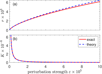
For small perturbation strength the eigenvalue change in Eq. (38) is small, therefore in Eq. (40) only the -term contributes, and consequently the denominator goes to unity. Hence, with Eq. (36) follows
| (41) |
in accordance with the general theoretical result in Eq. (28). Figure 2 shows a comparison of the exact result with the theoretical result for the phase rigidity and the Petermann factor . For small perturbation the agreement is nearly perfect.
VII Application
The computation of the spectral response strength of an EP of arbitrary order in Eq. (8) is easy and can be performed most of the time by hand. However, the equation requires the Hamiltonian to be an -matrix, which is a severe limitation. The same is true for the alternative computation based on the last Jordan vector in Eq. (12). For the more general case of an EP of order embedded in an Hilbert space of dimension no method of computation has been presented yet.
It is natural to assume that the revealed connection of and with the spectral response strength is a local property, even though we cannot provide an analytical proof here. This would offer a strategy for the computation of in the higher dimensional case. Let us consider an -Hamiltonian with an EP with order and eigenvalue . We perturb this system slightly by a randomly selected perturbation, which is with probability 1 a generic perturbation. The strength of which is a parameter of the method and has to be chosen to be large enough to move the system away from the EP. Otherwise would diverge and vanishes and therefore Eqs. (28) and (29) could not be used. At the same time the perturbation strength should be small enough such that the leading-order approximation which led to Eqs. (28) and (29) is still valid. Note that already the numerical implementation, even if double-precision floating-point arithmetic is used, can drive the system significant away from a higher-order EP [53]. In such a case no additional random perturbation is needed. For simplicity we assume that no other EP with eigenvalue close to exists. The method starts with computing all eigenvalues , right eigenstates , and left eigenstates of the Hamiltonian by a standard numerical routine. Next, the eigenstates and eigenvalues that are associated with the desired EP are selected. To do so, we determine from the set of eigenstates with small the quantum number for which the deviation is minimal. This minimum energy deviation we denote as . Finally, we plug and the corresponding phase rigidity into the equation for the numerically determined spectral response strength
| (42) |
which has been obtained from Eq. (28).
We demonstrate in the following that this simple scheme is quite efficient. To produce many numerical examples, we adopt the random-matrix approach invented in Ref. [39]. We introduce the matrix having an EP with order and eigenvalue via a similarity transformation , with being an matrix with an EP of order in Jordan normal form and is an, in general nonunitary, matrix consisting of complex random numbers with real and imaginary parts being drawn from a uniform distribution on the interval . We calculate the associated spectral response strength simply from Eq. (8) and save the value for later comparison. Subsequently, we create the -matrix with its elements to be complex random numbers with real and imaginary parts being drawn from a uniform distribution on . In the end, we combine these two matrices to obtain the Hamiltonian
| (43) |
The random unitary matrix is generated with the help of a QR decomposition of a random complex -matrix [56] constructed in the same way as above. The resulting Hamiltonian has an EP with the same eigenvalue , the same spectral response strength , and the same order than the original Hamiltonian . We find that the small numerical errors in the above procedure (double-precision floating-point arithmetic in MATLAB is used) drive slightly away from the EP. Hence, no additional random perturbation is needed here. The Hamiltonian is the input of the proposed scheme to compute the spectral response strength of the EP.
Using MATLAB the proposed procedure is illustrated in Fig. 3. In Fig. 3(a) the Hamiltonian in Eq. (43) is shown before the random unitary matrix is applied. In the colormap the submatrix appears darker than the submatrix because the former originates from the matrix where the matrix elements are 0 or 1 whereas the latter has random matrix elements in . Figure 3(b) depicts the Hamiltonian in Eq. (43) after the unitary transformation. The Hamiltonian looks random but it still possesses the EP inherited from with the same spectral response strength (up to numerical uncertainties).
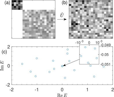
Figure 3(c) shows the eigenvalues of . The magnification in the inset reveals that the EP is slightly perturbed due to numerical uncertainties which lifts the degeneracy and results into a ring of five eigenvalues. This small splitting is essential for the proposed numerical scheme. As a side remark it is briefly mentioned that the appearance of the splitting of EP eigenvalues due to numerical uncertainties or fabrication imperfection is reminiscent to the vortex-splitting phenomenon [57] due to the instability of higher-order optical vortices.
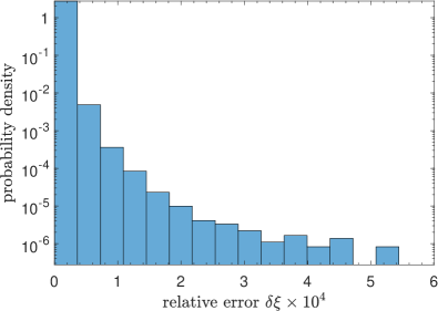
Figure 4 shows such a comparison for as many as realizations of Hamiltonians each very close to an EP of third order. The relative error is below one-tenth of a percent. The raw data (not shown) unveil that the largest deviations occur whenever the eigenvalue splitting due to the finite machine precision is relatively pronounced. Here the leading-order contribution may not always be sufficient for calculating the phase rigidity accurately enough. This happens in particular for larger order where small perturbations lead to large splittings. We observe relative errors around and below for (not shown). Our numerics demonstrate that the connection between phase rigidity and spectral response strength can be exploited to compute the latter even for the case where the dimension of the Hilbert space is larger than the order of the EP.
The introduced scheme for the computation of the spectral response strength could possibly be also applied to systems where no (effective) Hamiltonian is available but instead a wave equation, e.g., for optical microcavities [58], where the Petermann factors can be directly calculated from the spatial mode structure [10]. Based on the knowledge gained from the presented theory, we can interpret the fitting procedure in Ref. [59] to determine numerically the internal backscattering coefficient in a perturbed microdisk system (the absolute value is in this context) near a second-order EP as a special case of our scheme; the same for the recently published fitting procedure in Ref. [60]. Once again, it is emphasized that our approach is much more general as it applies to a wide range of systems and EPs of arbitrary order. A good test system for applying the above scheme would be the situation in Refs. [61, 62] where both a wave equation and an effective Hamiltonian are available simultaneously.
VIII Conclusion
We have derived explicit formulas for the Petermann factors and phase rigidities near EPs of arbitrary order. Our results not only confirm the known scaling behavior for generic perturbations but also provide the prefactor. Our theory has revealed an unexpected relation to the spectral response strength of the EP. Bounds for the Petermann factors and phase rigidities have been introduced that can be used for an easy estimation of the order of magnitude and in the case of passive systems allow for an assessment of the possibilities for enhanced sensing. We have discussed our results in the context of numerical studies in the literature. The predictions of our general theory have been compared to the solutions of an analytically solvable model and very good agreement has been observed.
We have demonstrated that the established connection of Petermann factors and phase rigidities with the spectral response strength can be exploited for the numerical computation of the latter even in the case of a higher-dimensional Hilbert space. The method is efficient and reliable for EPs with order up to five for double-precision floating-point arithmetic. EPs with even higher order are so sensitive to numerical imperfections that the highest-order contribution of the Green’s function is not always sufficient.
Realizing EPs experimentally is not an easy task in particular for EPs of higher order because of their extreme sensitivity to fabrication imperfections. In practice, the experimental setup is never located exactly on the EP but at best in its vicinity. Our theory of the Petermann factors and phase rigidities is able to predict of what is left of the sensitivity for such imperfect EPs. This is a valuable information for sensing applications. This applies in particular to experiments which are deliberately detuned from the EP to mitigate the harmful effects of quantum excess noise [38].
Moreover, our results can be beneficial for the study of extreme dynamics near higher-order EPs [63].
Acknowledgements.
Fruitful discussions with M. P. van Exter and H. Schomerus are acknowledged.Appendix A Computation of
This Appendix contains a short proof of Eq. (26). For the case we can write according to Eq. (5)
| (44) |
With the definition of the operator in Eq. (3) it is clear that
| (45) |
Hence,
| (46) |
In words, is orthogonal to all Jordan vectors for . The last Jordan vector is also orthogonal to all other Jordan vectors because of the chosen orthogonalization conditions in Eq. (7). We conclude that the unit vector is parallel (up to a complex phase) to and hence . Together with Eq. (46) this proves Eq. (26).
References
- Feshbach [1958] H. Feshbach, Unified theory of nuclear reactions, Ann. Phys. (N.Y.) 5, 357 (1958).
- Feshbach [1962] H. Feshbach, A unified theory of nuclear reactions. ii, Ann. Phys. (N.Y.) 19, 287 (1962).
- El-Ganainy et al. [2018] R. El-Ganainy, K. G. Makris, M. Khajavikhan, Z. H. Musslimani, and D. N. Christodoulides, Non-Hermitian physics and PT symmetry, Nat. Phys. 14, 11 (2018).
- Özdemir et al. [2019] Ş. K. Özdemir, S. Rotter, F. Nori, and L. Yang, Parity–time symmetry and exceptional points in photonics, Nat. Mater. 18, 783 (2019).
- Petermann [1979] K. Petermann, Calculated spontaneous emission factor for double-heterostructure injection lasers with gain-induced waveguiding, IEEE J. Quantum Electron. 15, 566 (1979).
- Siegman [1989a] A. E. Siegman, Excess spontaneous emission in non-Hermitian optical systems. I. Laser amplifiers, Phys. Rev. A 39, 1253 (1989a).
- Siegman [1989b] A. E. Siegman, Excess spontaneous emission in non-Hermitian optical systems. II. Laser oscillators, Phys. Rev. A 39, 1264 (1989b).
- Siegman [1995] A. E. Siegman, Lasers without photons - or should it be lasers with too many photons?, Appl. Phys. B 60, 247 (1995).
- van der Lee et al. [1998] A. M. van der Lee, M. P. van Exter, A. L. Mieremet, N. J. van Druten, and J. P. Woerdman, Excess Quantum Noise is Colored, Phys. Rev. Lett. 81, 5121 (1998).
- Schomerus [2009] H. Schomerus, Excess quantum noise due to mode nonorthogonality in dielectric microresonators, Phys. Rev. A 79, 061801(R) (2009).
- Wang et al. [2020] H. Wang, Y.-H. Lai, Z. Yuan, M.-G. Suh, and K. Vahala, Petermann-factor sensitivity limit near an exceptional point in a Brillouin ring laser gyroscope, Nat. Commun. 11, 1610 (2020).
- Schomerus [2020] H. Schomerus, Nonreciprocal response theory of non-Hermitian mechanical metamaterials: Response phase transition from the skin effect of zero modes, Phys. Rev. Res. 2, 013058 (2020).
- Budich and Bergholtz [2020] J. C. Budich and E. J. Bergholtz, Non-Hermitian Topological Sensors, Phys. Rev. Lett. 125, 180403 (2020).
- Nakai et al. [2023] Y. O. Nakai, N. Okuma, D. Nakamura, K. Shimomura, and M. Sato, Topological enhancement of non-normality in non-Hermitian skin effects, arXiv:2304.06689 10.48550/arXiv.2304.06689 (2023).
- Bauer and Fike [1960] F. L. Bauer and C. T. Fike, Norms and exclusion theorems, Numer. Math. 2, 137 (1960).
- Trefethen and Embree [2005] L. N. Trefethen and M. Embree, Spectra and Pseudospectra (Princeton University Press, Princeton, NJ, 2005).
- van der Lee et al. [1997] A. M. van der Lee, N. J. van Druten, A. L. Mieremet, M. A. van Eijkelenborg, Å. M. Lindberg, M. P. van Exter, and J. P. Woerdman, Excess Quantum Noise due to Nonorthogonal Polarization Modes, Phys. Rev. Lett. 79, 4357 (1997).
- Ding et al. [2016] K. Ding, G. Ma, M. Xiao, Z. Q. Zhang, and C. T. Chan, Emergence, Coalescence, and Topological Properties of Multiple Exceptional Points and Their Experimental Realization, Phys. Rev. X 6, 021007 (2016).
- Xiao et al. [2019a] Y.-X. Xiao, Z.-Q. Zhang, Z. H. Hang, and C. T. Chan, Anisotropic exceptional points of arbitrary order, Phys. Rev. B 99, 241403(R) (2019a).
- Jaiswal et al. [2023] R. Jaiswal, A. Banerjee, and A. Narayan, Characterizing and tuning exceptional points using Newton polygons, New J. Phys. 10.1088/1367-2630/acc1fe (2023).
- van Langen et al. [1997] S. A. van Langen, P. W. Brouwer, and C. W. J. Beenakker, Fluctuating phase rigidity for a quantum chaotic system with partially broken time-reversal symmetry, Phys. Rev. E 55, R1 (1997).
- Bulgakov et al. [2006] E. N. Bulgakov, I. Rotter, and A. F. Sadreev, Phase rigidity and avoided level crossings in the complex energy plane, Phys. Rev. E 74, 056204 (2006).
- Rotter [2015] I. Rotter, A review of progress in the physics of open quantum systems: theory and experiment, Rep. Prog. Phys. 78, 114001 (2015).
- Jin [2018] L. Jin, Parity-time-symmetric coupled asymmetric dimers, Phys. Rev. A 97, 012121 (2018).
- Zhang et al. [2020] S. M. Zhang, X. Z. Zhang, L. Jin, and Z. Song, Higher-order exceptional points in supersymmetric arrays, Phys. Rev. A 101, 033820 (2020).
- Sadreev and Berggren [2005] A. F. Sadreev and K.-F. Berggren, Signatures of quantum chaos in complex wave functions describing open billiards, J. Phys. A: Math. Gen. 38, 10787 (2005).
- Kato [1966] T. Kato, Perturbation Theory for Linear Operators (Springer, New York, 1966).
- Heiss [2000] W. D. Heiss, Repulsion of resonance states and exceptional points, Phys. Rev. E 61, 929 (2000).
- Berry [2004] M. V. Berry, Physics of nonhermitian degeneracies, Czech. J. Phys. 54, 1039 (2004).
- Heiss [2004] W. D. Heiss, Exceptional points of non-Hermitian operators, J. Phys. A: Math. Gen. 37, 2455 (2004).
- Miri and Alù [2019] M.-A. Miri and A. Alù, Exceptional points in optics and photonics, Science 363, eaar7709 (2019).
- Wiersig [2014] J. Wiersig, Enhancing the Sensitivity of Frequency and Energy Splitting Detection by Using Exceptional Points: Application to Microcavity Sensors for Single-Particle Detection, Phys. Rev. Lett. 112, 203901 (2014).
- Chen et al. [2017] W. Chen, Ş. K. Özdemir, G. Zhao, J. Wiersig, and L. Yang, Exceptional points enhance sensing in an optical microcavity, Nature (London) 548, 192 (2017).
- Hodaei et al. [2017] H. Hodaei, A. Hassan, S. Wittek, H. Carcia-Cracia, R. El-Ganainy, D. Christodoulides, and M. Khajavikhan, Enhanced sensitivity at higher-order exceptional points, Nature (London) 548, 187 (2017).
- Xiao et al. [2019b] Z. Xiao, H. Li, T. Kottos, and A. Alù, Enhanced sensing and nondegraded thermal noise performance based on PT-symmetric electronic circuits with a sixth-order exceptional point, Phys. Rev. Lett. 123, 213901 (2019b).
- Wiersig [2020a] J. Wiersig, Prospects and fundamental limits in exceptional point-based sensing, Nat. Commun. 11, 2454 (2020a).
- Wiersig [2020b] J. Wiersig, Review of exceptional point-based sensors, Photonics Res. 8, 1457 (2020b).
- Kononchuk et al. [2022] R. Kononchuk, J. Cai, F. Ellis, R. Thevamaran, and T. Kottos, Exceptional-point-based accelerometers with enhanced signal-to-noise ratio, Nature (London) 607, 697 (2022).
- Wiersig [2022a] J. Wiersig, Response strengths of open systems at exceptional points, Phys. Rev. Res. 4, 023121 (2022a).
- Moiseyev and Friedland [1980] N. Moiseyev and S. Friedland, Association of resonance states with the incomplete spectrum of finite complex-scaled Hamiltonian matrices, Phys. Rev. A 22, 618 (1980).
- Moiseyev [2011] N. Moiseyev, Non-Hermitian Quantum Mechanics (Cambridge University Press, Cambridge, 2011).
- Berry [2003] M. V. Berry, Mode degeneracies and the Petermann excess-noise factor for unstable lasers, J. Mod. Optics 50, 63 (2003).
- Lee et al. [2008] S.-Y. Lee, J.-W. Ryu, J.-B. Shim, S.-B. Lee, S. W. Kim, and K. An, Divergent Petermann factor of interacting resonances in a stadium-shaped microcavity, Phys. Rev. A 78, 015805 (2008).
- Lee [2009] S.-Y. Lee, Decaying and growing eigenmodes in open quantum systems: Biorthogonality and the Petermann factor, Phys. Rev. A 80, 042104 (2009).
- Zheng et al. [2010] M. C. Zheng, D. N. Christodoulides, R. Fleischmann, and T. Kottos, PT optical lattices and universality in beam dynamics, Phys. Rev. A 82, 010103(R) (2010).
- Mostafavi et al. [2020] F. Mostafavi, C. Yuce, O. S. Maganã-Loaiza, H. Schomerus, and H. Ramezani, Robust localized zero-energy modes from locally embedded PT-symmetric defects, Phys. Rev. Res. 2, 032057(R) (2020).
- Heiss [2008] W. D. Heiss, Chirality of wavefunctions for three coalescing levels, J. Phys. A: Math. Theor. 41, 244010 (2008).
- Seyranian and Mailybaev [2003] A. P. Seyranian and A. A. Mailybaev, Multiparameter Stability Theory with Mechanical Applications (Singapore, World Scientific, 2003).
- Horn and Johnson [2013] R. A. Horn and C. R. Johnson, Matrix Analysis (Cambridge University Press, Cambridge, 2013).
- Mandal and Bergholtz [2021] I. Mandal and E. J. Bergholtz, Symmetry and Higher-Order Exceptional Points, Phys. Rev. Lett. 127, 186601 (2021).
- Sayyad and Kunst [2022] S. Sayyad and F. K. Kunst, Realizing exceptional points of any order in the presence of symmetry, Phys. Rev. Res. 4, 023130 (2022).
- Chalker and Mehlig [1998] J. T. Chalker and B. Mehlig, Eigenvector Statistics in Non-Hermitian Random Matrix Ensembles, Phys. Rev. Lett. 81, 3367 (1998).
- Wiersig [2022b] J. Wiersig, Revisiting the hierarchical construction of higher-order exceptional points, Phys. Rev. A 106, 063526 (2022b).
- Wiersig [2022c] J. Wiersig, Distance between exceptional points and diabolic points and its implication for the response strength of non-Hermitian systems, Phys. Rev. Research 4, 033179 (2022c).
- Hatano and Nelson [1996] N. Hatano and D. R. Nelson, Localization Transitions in Non-Hermitian Quantum Mechanics, Phys. Rev. Lett. 77, 570 (1996).
- Mezzadri [2007] F. Mezzadri, How to generate random matrices from the classical compact groups, Not. Am. Math. Soc. 54, 592 (2007).
- Ricci et al. [2012] F. Ricci, W. Löffler, and M. P. van Exter, Instability of higher-order optical vortices analyzed with a multi-pinhole interferometer, Opt. Express 20, 22961 (2012).
- Wiersig [2003] J. Wiersig, Boundary element method for resonances in dielectric microcavities, J. Opt. A: Pure Appl. Opt. 5, 53 (2003).
- Wiersig [2016] J. Wiersig, Sensors operating at exceptional points: General theory, Phys. Rev. A 93, 033809 (2016).
- Kim et al. [2023] H. Kim, S. Gwak, H.-H. Yu, J. Ryu, C.-M. Kim, and C.-H. Yi, Maximization of frequency splitting on continuous exceptional points in asymmetric optical microdisks, Opt. Express 31, 12634 (2023).
- Kullig et al. [2018] J. Kullig, C.-H. Yi, and J. Wiersig, Exceptional points by coupling of modes with different angular momenta in deformed microdisks: A perturbative analysis, Phys. Rev. A 98, 023851 (2018).
- Kullig and Wiersig [2019] J. Kullig and J. Wiersig, High-order exceptional points of counterpropagating waves in weakly deformed microdisk cavities, Phys. Rev. A 100, 043837 (2019).
- Zhong et al. [2018] Q. Zhong, D. N. Christodoulides, M. Khajavikhan, K. G. Makris, and R. El-Ganainy, Power-law scaling of extreme dynamics near higher-order exceptional points, Phys. Rev. A 97, 020105(R) (2018).