Improving Autoencoder-based Outlier Detection with Adjustable Probabilistic Reconstruction Error and Mean-shift Outlier Scoring

Abstract

Autoencoders were widely used in many machine learning tasks thanks to their strong learning ability which has drawn great interest among researchers in the field of outlier detection. However, conventional autoencoder-based methods lacked considerations in two aspects. This limited their performance in outlier detection. First, the mean squared error used in conventional autoencoders ignored the judgment uncertainty of the autoencoder, which limited their representation ability. Second, autoencoders suffered from the abnormal reconstruction problem: some outliers can be unexpectedly reconstructed well, making them difficult to identify from the inliers. To mitigate aforementioned issues, two novel methods were proposed in this paper. First, a novel loss function named Probabilistic Reconstruction Error (PRE) was constructed to factor in both reconstruction bias and judgment uncertainty. To further control the trade-off of these two factors, two weights were introduced in PRE producing Adjustable Probabilistic Reconstruction Error (APRE), which benefited the outlier detection in different applications. Second, a conceptually new outlier scoring method based on mean-shift (MSS) was proposed to reduce the false inliers caused by the autoencoder. Experiments on 32 real-world outlier detection datasets proved the effectiveness of the proposed methods. The combination of the proposed methods achieved 41% of the relative performance improvement compared to the best baseline. The MSS improved the performance of multiple autoencoder-based outlier detectors by an average of 20%. The proposed two methods have the potential to advance autoencoder’s development in outlier detection. The code is available on www.OutlierNet.com for reproducibility.

I Introduction

Outlier detection (OD), also known as anomaly detection, is a fundamental technique in the field of data mining. An outlier can be defined as ”one that appears to deviate markedly from other members of the sample in which it occurs” [1]. Outliers exhibit two main properties: (1) different from the norm with respect to their features; (2) rare in a dataset compared to normal samples [2]. The target of OD is to identify the outliers from the normal samples (inliers), to keep the data clean and safe, or identify the abnormal situations and behaviors. OD is widely used in many applications, such as fraud detection [3, 4, 5], network intrusion detection [6, 7], medical anomaly diagnosis [8, 9, 10], video surveillance [11, 12, 13] and trajectory analysis [14, 15, 16].

Numerous OD methods have been proposed over the years. They could be categorized into different classes. Proximity-based methods [17, 18, 19, 20, 21, 22] measured the similarities between inliers and outliers in the original data space. Statistical-based methods [23, 24, 25] modeled the statistic distribution of inliers. Classification-based methods [26, 27, 28] transformed the data to another space before identifying outliers by dividing the space. Ensemble-based methods [29, 30, 31, 32] utilized the stochasticity and diversity of data, then combined several weak outlier detectors into a strong detector. Probabilistic-based methods [33, 34] analyzed the probabilistic distribution of the attributes of the data.

In recent years, deep learning techniques have piqued the curiosity of experts in many fields including OD. Learning-based methods, such as autoencoder-based (AE-based) [35, 36, 37, 38, 39, 40] and generative-adversarial-network-based (GAN-based) [9, 41, 42, 43], utilized the strong learning ability of the neural network to learn the inherent pattern of the inliers. AE-based methods assumed that the inliers could be reconstructed better than the outliers. GAN-based methods learned to create outliers through the generator or distinguish between inliers and outliers through the discriminator. Generally, GAN-based methods are hard to train because of their adversarial property, thus AE-based methods are the most popular among all learning-based methods at present [44]. However, conventional AE-based methods lacked considerations in two aspects, which limited their performance in outlier detection.

Firstly, almost all the AE-based methods utilized the reconstruction error, such as the mean square error, to detect outliers. However, these methods discounted the concept of uncertainty in AE, which is critical for AE’s training and judgment on outliers, and will be explained in detail in Sec. III-A. In this paper, we reveal the probabilistic nature of the AE, and provide a novel explanation of the AE-based OD methods: the fundamental assumptions made by AE were that outliers had larger reconstruction bias and greater judgment uncertainty than inliers. Specifically, the mean squared error (MSE) was derived using the probability theory. Then it was found that, the optimization of MSE was equivalent to the maximization of the logarithmic probability density function, assuming that the reconstruction variance of each attribute was one. The assumption simplified the optimization of the loss function, but limited the learning ability of the AE: a well-learned AE should reconstruct the input with both minimal bias and uncertainty.

To tackle the limitation, we propose a novel loss function Probabilistic Reconstruction Error (PRE), which considers the bias and uncertainty simultaneously, to maximize AE’s potential for learning to output a more precise reconstruction. PRE also improves AE’s ability of detecting outliers, since outliers may be identified with greater ease when considering both bias and uncertainty, as compared to just bias. To further adjust the effects of the bias and uncertainty in different OD applications, two adjustable scaling hyper-parameters were added to modify PRE, producing a scoring function. This method was termed Adjustable Probabilistic Reconstruction Error (APRE). The flexibility of the weights adjusting makes it effective for different OD scenarios.

Secondly, conventional AE-based OD methods suffered from the abnormal reconstruction problem. That is, some outliers can be unexpectedly reconstructed well, making them difficult to identify from the inliers [45]. This phenomenon can be explained by the fact that conventional AE only captured global features of data, lacking explicit consideration of local information. In this paper, we mitigate the issue by modifying the scoring strategy of AE, producing the Mean-Shift outlier Scoring (MSS) method. This method uses the mean-shifted data point instead of the original data point to calculate the outlier scores. Thus, when an outlier is reconstructed with a relatively high probability, the reconstruction result will not appear to the mean-shifted result of the input, leading to a high outlier score. This method is convenient and effective, and is quite generalized that it can be applied to most AE-based methods easily, which will be shown in Sec. IV.

A demonstration of the complete outlier scoring process of the typical AE-based OD methods, AE with the proposed APRE, and AE with the proposed MSS was shown in Fig. 1. The AE with APRE used APRE as the score function, and the AE-based model was trained using PRE. The AE with MSS used the mean-shifted data to compute the score function, and the final function depended on the base function, such as MSE or APRE.

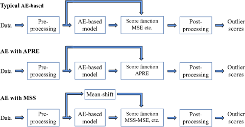
Figure 1: A demonstration of the complete outlier scoring process of the typical AE-based methods, AE with the proposed APRE, and AE with the proposed MSS.

In summary, the main contributions of this work are as follows:

• Proposing the PRE, a novel loss function for AE-based methods that can improve the learning ability of the AE.

• Proposing the APRE, the weighted version of PRE. The flexibility of the weights adjusting makes it effective for different OD applications.

• Proposing the MSS, which is a convenient and effective scoring method that can improve the robustness and accuracy of AE. In addition to its efficacy, it can be easily applied to most AE-based methods.

• Conducting experiments on 32 real-world OD datasets, comparing the proposed methods with 5 typical AE-based OD methods and 5 classic state-of-the-art (SOTA) OD methods. The experimental results proved the effectiveness and superiority of our methods.

The rest of the paper is organized as follows: In Sec. II, the concept of AE for OD and some typical AE-based outlier detection methods proposed in recent years are reviewed. In Sec. III, the proposed PRE, APRE, and MSS method are introduced in detail, and their theoretical advantages are analyzed. The practical implementation details are also described in this section. Then the experimental settings are described and the results are reported in Sec. IV. A discussion of the proposed methods is presented in Sec. V. Finally, a conclusion is drown in Sec. VI.

II Related Work

II-A Autoencoder for outlier detection

An AE is a neural network that is trained to reproduce its input to its output [46]. It comprises of two main components: the encoder and the decoder. Considering a traditional fully-connected AE, given a multivariate data vector $\mathbf{x}\in\mathbb{R}^{D}$ as the input, the encoder transforms it to a lower-dimensional latent representation, which retains the most critical features of the input data. The latent representation $\mathbf{z}$ output by the encoder is given as

$$\mathbf{z}={\rm Encoder}(\mathbf{x},\theta),$$ (1)

where $\theta$ denotes the network parameters of the encoder. Then, the decoder reconstructs the input using the latent representation and the decoder output is expressed as

$$\hat{\mathbf{x}}={\rm Decoder}(\mathbf{z},\phi),$$ (2)

where $\hat{\mathbf{x}}$ denotes the output of AE and $\phi$ denotes the network parameters of the decoder.

Since the fully-connected layer can be viewed as the linear dimensionality reduction transformation, the effect of the encoder is similar to the principle components analysis, which aims to find the main components reflecting the features of the original data [47]. However, the complicated real-world data are difficult to analyze linearly, so a nonlinear activation function is applied after each fully-connected layer to increase the expressiveness of the network. Common typical activation functions are Sigmoid, Tanh, Rectified Linear Unit (ReLU), and ReLU’s variants.

The optimization and outlier score computation of an AE both relies on its loss function. Since the target of the AE is to reconstruct the input data as the output, the bias between the input and output can naturally be used as the loss function. This is also known as the reconstruction error. The most popular loss function of the conventional AE is the Mean Squared Error (MSE) loss, which is established as

$${\rm MSE}(\mathbf{x},\hat{\mathbf{x}})=||\mathbf{x}-\hat{\mathbf{x}}||_{2}^{2},$$ (3)

where $||\cdot||_{2}$ denotes the L2-norm.

As introduced above, an AE first transforms the input $\mathbf{x}$ to the latent $\mathbf{z}$, then transforms $\mathbf{z}$ to the output $\hat{\mathbf{x}}$. The dimension of the latent presentation $\mathbf{z}$ is designed to be smaller than the input layer. It served as a bottleneck layer, allowing only the most important information to pass through [48]. Thus, the AE is forced to capture the most critical features of the data to better reconstruct the input.

Considering a dataset that contains both inliers and outliers. Inliers are abundant and generally showed similar patterns, thus their features can easily be learned by an AE. Outliers are few and different in the dataset, hence their features are difficult for an AE to summarize. As a consequence, inliers can be reconstructed with low errors by the AE, but high reconstruction errors for outliers.

II-B Autoencoder-based outlier detection methods

In this section, some typical AE-based outlier detection methods proposed in recent years are reviewed.

Zhou et al. proposed the Robust Deep Autoencoders (RDA) [36], motivated by the robust principal component analysis. RDA split the input data $\mathbf{X}$ into two parts $\mathbf{X}=\mathbf{L}_{D}+\mathbf{S}$, where $\mathbf{L}_{D}$ represented the part that could be well-reconstructed by the AE, and $\mathbf{S}$ contained the noise and outliers which were difficult to reconstruct. The loss function of RDA had two parts: the reconstruction error of $\mathbf{L}_{D}$ and the sparse penalty on $\mathbf{S}$, which were optimized alternately during training. This ensured that anomalous components were iteratively removed from the training set. By isolating the noise or outliers and putting them into $\mathbf{S}$, RDA kept the AE training from the contaminated data components, making the model robust. In addition, the outlier score of a sample could be measured by the length of its noise component $||\mathbf{s}||$. The authors also proposed the $l_{2,1}$ regularization, which could penalize the outliers and anomalous features in the training data simultaneously.

Chen et al. proposed the Randomized Neural Network for Outlier Detection (RandNet) [49] to improve the robustness of AE. RandNet generated several randomly connected AEs, i.e., some of the neural connections in the network were randomly dropped. Then, the AEs were trained with different sampling sets of the full dataset to overfit the subsets. Finally, the outlier scores (i.e., the reconstruction error generated by these AEs) were combined into the final score. RandNet was a typical ensemble learning method that combined several weak but different detectors to form a strong detector. The randomness of the network architectures and the composition of the training sets increased the diversity of the sub-detectors.

An et al. proposed a variational-autoencoder-based (VAE-based) OD method with a novel loss function [37]. A VAE was a probabilistic graphical model that combined variational inference with deep learning. The model induced the latent representation of an AE to map a prior disentangled distribution, such as the centered isotropic multivariate Gaussian distribution, to get disentangled features in the latent space. Apart from using the VAE, the authors also proposed to estimate the reconstruction probability of the reconstruction data, which was more principled and objective than the general reconstruction error.

Ishii et al. proposed the Low-Cost Autoencoder (LCAE), introducing a training trick for AE-based OD methods. It incorporated the concepts of the least trimmed squares (LTS) estimator [50]. The trick restricted the reconstruction capability and ensured the robustness of the AE. In addition, LTS also reduced the computational cost. Samples with higher reconstruction errors were more likely to be outliers, detrimental to AE training. Thus, samples with high reconstruction errors (e.g. top 30% of the highest errors) were not used for updating parameters during training. To achieve this, these samples had their losses annulled and reset to 0.

Gong et al. proposed a Memory-augmented Autoencoder (MemAE) [51]. The purpose of the method was to improve the robustness of the AE by reconstructing samples from a limited number of recorded representative normal patterns. To achieve that, the authors added a size-restricted memory module between the encoder and decoder. Then, the decoder took the combination of the items in the memory module as input, instead of the encoded features. In the training phase, the memory module was trained to record several representative prototypical patterns by using only inliers. In the testing phase, the memory was fixed to ensure that only the recorded normal patterns can be retrieved for reconstruction. Thus, the inliers could naturally be reconstructed well, but the outliers were obviously more difficult to reconstruct from the normal patterns.

Lai et al. proposed an AE model based on the Robust Subspace Recovery layer (RSRAE) [38]. The RSR layer was a linear transformation added between the general encoder and decoder, which further reduced the dimension of the latent representation generated by the encoder. The effect of the RSR layer could be viewed as an orthogonal projection that projected latent features into a subspace. From this subspace, latent features could be recovered again, especially normal features. The authors observed that recovery of outliers from the subspace was more difficult compared to inliers, thus improving the AE’s ability of distinguishing between the outliers and inliers.

Similarly, Yu et al. also utilized the subspace technique to propose an improved AE based on orthogonal projection constraints (OPCAE)[52]. Specifically, the authors used the anomaly-free data to compute a Kautlr-Thomas transformation (also known as K-T transformation, Tctasseled cap transformation), and induced a network (comprised of two consecutive linear transformation layers) to approach the K-T transformation. The network was added between the general encoder and decoder, which could be viewed as an extra transformation applied to the latent representation generated by the encoder. The authors highlighted that, the feature after the transformation was expected to contain only the normal information, thus providing an advantage for distinguishing outliers and inliers.

Guo et al. proposed an AE architecture called Feature Decomposition Autoencoder (FDAE) [39], which integrated the RDA [36] and RSRAE [38]. FDAE had one encoder followed by two sub-nets. The first sub-net contained an RSR layer and a decoder, while the second sub-net contained a noise extractor and another decoder. The RSR layer and noise extractor divided the encoding representation into normal features and abnormal features. Then, two decoders output the normal component and abnormal component of the input data respectively, which were similar to $\mathbf{L}_{D}$ and $\mathbf{S}$ in [36]. The loss function of FDAE was complicated, which included the optimization of the reconstruction error, the RSR layer, and the complementarity of the normal and abnormal parts.

Angiulli et al. proposed a novel AE-based framework called LatentOut [40], which considered the relative position relationship of data in the latent space. Specifically, LatentOut concatenated the latent representation and the reconstruction error of the AE as a new feature vector, and computed its $k$-nearest-neighbors ($k$-NN) distance as the outlier score. The framework was effective in circumstances where the reconstruction errors of some regions (including inliers and outliers) were higher than that in other regions.

TABLE I: Main improved components and features of the recent typical AE-based OD methods and the proposed methods.

Method	Model	Training	Score	Feature
RDA	✓	✓	✓	Component decomposition
RandNet	✓	✓		Ensemble
VAE	✓	✓	✓	Variational Inference
LCAE		✓		Least trimmed
MemAE	✓	✓		Pattern storage
RSRAE	✓	✓		Feature subspace
OPCAE	✓	✓	✓	Latent transformation
FDAE	✓	✓		Feature decomposition
LatentOut			✓	Latent analysis
PRE+APRE	✓	✓	✓	Probability analysis
MS-			✓	Auxiliary scoring

To summarize, the majority of recent AE-based methods have focused on enhancing AE’s robustness and ability to represent data, enabling easier differentiation between inliers and outliers. These methods have various improved components and distinct features, which were summarized in Table I. However, they have mostly neglected the uncertainty factor discussed earlier. An et al. [37] integrated reconstruction mean and variance to the reconstruction probability, but they did not analyze them theoretically or decompose the two factors to balance their impact in different applications. Moreover, these methods are often complex in their mechanisms, hindering collaborative efforts with other techniques.

In this paper, two methods were proposed to mitigate the aforementioned issues and improve AE’s OD ability. First, the PRE considering the reconstruction bias and judgment uncertainty of the AE simultaneously was proposed with a theoretical analysis. A weighting strategy was applied to PRE producing APRE which was flexible for different applications. Second, the MSS was proposed as a universal scoring method that could be easily plugged into other AE-based OD methods to improve their performance. They are introduced in detail in Sec. III.

III Methodology

In this section, the proposed PRE, APRE, and MSS method will be introduced in detail.

III-A Adjustable Probabilistic Reconstruction Error

To introduce the proposed PRE and APRE function, the loss function of the conventional AE will be derived from the probability perspective. Then it will be proved that the mechanism of AE can be explained as predicting the reconstruction probability distribution of the input $\mathbf{x}$ as follows. Assuming the distribution is the isotropic multivariate Gaussian distribution, Eq. 4 is established:

$$\left\{\begin{aligned} &\mathbf{x}^{\rm rec}\sim{\rm N}(\bm{\mu},\bm{\Sigma}),\\ &\bm{\mu}=[\mu_{1},\mu_{2},\cdots,\mu_{D}]^{T},\\ &\bm{\sigma}^{2}=[\sigma_{1}^{2},\sigma_{2}^{2},\cdots,\sigma_{D}^{2}]^{T},\\ &\bm{\Sigma}={\rm diag}(\bm{\sigma}^{2}),\end{aligned}\right.$$ (4)

where $\mathbf{x}^{\rm rec}$ denotes the reconstruction random variable of input $\mathbf{x}$; ${\rm diag}(\cdot)$ denotes the diagonal matrix; $\bm{\mu}$ denotes the reconstruction mean of AE, which reflects the reconstruction result of AE; $\bm{\sigma}$ denotes the reconstruction standard deviation, which reflects AE’s uncertainty for the accuracy of the reconstruction result. This gives rise to Eq. 5:

$$P(\mathbf{x}^{\rm rec})=\frac{1}{(2\pi)^{D/2}}\frac{1}{|\bm{\Sigma}|^{1/2}}e^{-\frac{1}{2}(\mathbf{x}^{\rm rec}-\bm{\mu})^{T}\bm{\Sigma}^{-1}(\mathbf{x}^{\rm rec}-\bm{\mu})},$$ (5)

where $P(\cdot)$ denotes the probability density function, $|\bm{\Sigma}|$ denotes the determinant of the matrix $\bm{\Sigma}$, and $\bm{\Sigma}^{-1}$ denotes the inverse matrix of $\bm{\Sigma}$. The logarithmic probability density function may be expressed as Eq. 6:

$$\ln P(\mathbf{x}^{\rm rec})=-\frac{D}{2}\ln 2\pi-\frac{1}{2}\sum_{d=1}^{D}{\ln\sigma_{d}}-\frac{1}{2}\sum_{d=1}^{D}{\frac{(x_{d}^{\rm rec}-\mu_{d})^{2}}{\sigma_{d}}}.$$ (6)

If all standard deviation values are assumed to be 1, then

$$\sigma_{1}=\sigma_{2}=\cdots =\sigma_{D}=1,$$ (7)

$$\bm{\Sigma}= \mathbf{I},$$

where $\mathbf{I}$ denotes the identity matrix. Therefore, the logarithmic probability density function, also known as the log-likelihood of $\mathbf{x}^{\rm rec}$ can be expressed by Eq. 8:

$$\ln P(\mathbf{x}^{\rm rec}) =-\frac{D}{2}\ln 2\pi-\frac{1}{2}\sum_{d=1}^{D}{(x_{d}^{\rm rec}-\mu_{d})^{2}}$$ (8)

$$=C-\frac{1}{2}||\mathbf{x}^{\rm rec}-\bm{\mu}||_{2}^{2},$$

where $C$ denotes a constant which will not affect the optimization process.

Conventional AEs aim to reconstruct the input $\mathbf{x}$, which implies maximizing the log-likelihood $\ln P(\mathbf{x}^{\rm rec})$ when $\mathbf{x}^{\rm rec}=\mathbf{x}$, and the mean value $\bm{\mu}$ is treated as the output $\hat{\mathbf{x}}$ of AE. Therefore, the optimization objective is to maximize $C-\frac{1}{2}||\mathbf{x}-\hat{\mathbf{x}}||_{2}^{2}$. Evidently, it is equivalent to minimizing $||\mathbf{x}-\hat{\mathbf{x}}||_{2}^{2}$, which is just the component of the general MSE. So given the training set $\mathbf{X}\in\mathbb{R}^{N\times D}$, the loss function of the conventional AE can be represented by Eq. 9:

$${\rm MSE}(\mathbf{X},\hat{\mathbf{X}})=\sum_{i=1}^{N}{||\mathbf{x}_{i}-\hat{\mathbf{x}_{i}}||_{2}^{2}},$$ (9)

where $N$ denotes the number of samples in the training set.

AE                                       PAE

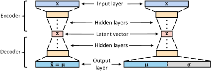
Figure 2: The typical structure of the AE and proposed PAE. For AE, the structure is symmetrical and the units of the hidden layers in the encoder decrease with successive layers. The difference is that PAE has a output layer twice the size of its input layer.

Experts on AE predominantly used the form of Eq. 8 or its variants, such as $||\cdot||_{2}$ (root mean squared error) or $||\cdot||_{1}$ (mean absolute error) as the loss function. However, as established prior in this text, the usage of the MSE loss is under the assumption that the standard deviation values $\bm{\sigma}$ of all the reconstruction probability distributions are 1. With this assumption, AE only estimates the mean values $\bm{\mu}$ of the distribution. The assumption simplifies the optimization of the loss function, but it also limits the AE’s learning ability: a well-learned AE should reconstruct the input with both minimal reconstruction bias and judgment uncertainty. Therefore, to fully explore the potential for AE to provide a good representation, this AE study estimates $\bm{\sigma}$ and combines it into a loss function simultaneously. To achieve this, the constant terms and coefficients in Eq. 6 were removed, forming Eq. 10, called PRE.

$${\rm PRE}(\mathbf{X},\bm{\mu},\bm{\sigma})=\sum_{i=1}^{N}{\sum_{d=1}^{D}{\frac{(x_{i,d}-\mu_{i,d})^{2}}{\sigma_{i,d}}}}+\sum_{i=1}^{N}{\sum_{d=1}^{D}{\ln\sigma_{i,d}}}.$$ (10)

where $x_{i,d}$, $\mu_{i,d}$ and $\sigma_{i,d}$ denote the $d$-th attribute of the sample $\mathbf{x}_{i}$, output mean values $\bm{\mu}_{i}$, and output standard deviation values $\bm{\sigma}_{i}$, respectively. The first term of PRE is referred to as the bias term, being similar to the squared mahalanobis distance, which measures the bias between the input data and the reconstruction distribution output by the AE. The second term is referred to as the uncertainty term, being the logarithmic output standard deviation, which measures the AE’s uncertainty on the reconstruction result ($\bm{\mu}$), thus termed as the uncertainty term. With this training loss function, AE not only aims to narrow the gap between the input data and the estimated mean values, but also tries to reduce the estimated variance to improve the certainty of the result.

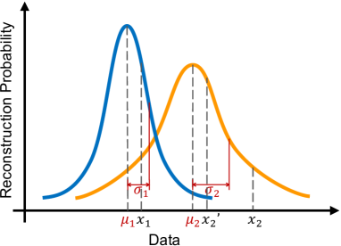
Figure 3: The reconstruction probability distribution of an inlier and an outlier. The blue curve denotes the inlier distribution and the orange curve denotes the outlier distribution. $x_{1}$ and $x_{2}$ denote the original inlier and outlier data respectively; $\mu_{1}$ and $\mu_{2}$ denote the reconstruction mean of the inlier and outlier respectively; $\sigma_{1}$ and $\sigma_{2}$ denote the reconstruction standard deviation of the inlier and outlier respectively. The outlier is expected to have larger bias ($||x_{2}-\mu_{2}||$ vs. $||x_{1}-\mu_{1}||$) and larger uncertainty ($\sigma_{2}$ vs. $\sigma_{1}$). Even if the outlier has similar bias compared to an inlier (e.g. $x_{2}^{\prime}$), it may be distinguishable by the uncertainty.

 

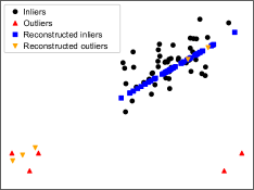
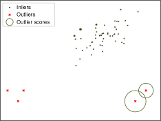
(a) Original data                     (b) Outlier scores computed

and data reconstructed by PAE.              by the bias term of APRE.

 

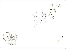
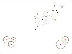
(c) Outlier scores computed              (d) Outlier scores computed

by the uncertainty term of APRE.       by APRE with {$\alpha=0.5$, $\beta=2$}.

Figure 4: A 2-D example of the effect of PRE and APRE. The original data included 50 2-D Gaussian-distributed inliers (black dots) and 5 outliers (red dots), as shown in (a). Then, PAE was trained using the data with the loss function of PRE. The reconstruction results for inliers (blue squares) and outliers (orange triangles) are reflected in (a). (b)-(d) showed the outlier scores generated by different scoring functions. The larger the radius of the green circle, the higher the outlier score. APRE succeed in detecting all outliers.

PRE also helps researchers understand AE’s ability of identifying outliers more deeply. Intuitively, AE is trained to capture the features of inliers, thus when AE tries to reconstruct an outlier, it can neither output the reconstruction accurately nor have sufficient faith in the result. Fig. 3 shows a demonstration of the reconstruction probability distribution of an inlier and an outlier. The blue curve denotes the inlier’s distribution and the orange curve denotes the outlier’s distribution. It is observed that the outlier is expected to have larger bias ($||\mathbf{x}_{2}-\mathbf{\mu}_{2}||$ vs. $||\mathbf{x}_{1}-\mathbf{\mu}_{1}||$) and larger uncertainty ($\mathbf{\sigma}_{2}$ vs. $\mathbf{\sigma}_{1}$). Moreover, even if an outlier has similar bias compared to an inlier, it may be distinguishable by the uncertainty and vice versa.

During the scoring phase, the bias term and uncertainty term both contributed to OD, but they had varying importance and thus different weightage for different applications. The two weighting hyper-parameters were added to control the trade-off of the two terms:

$$\text{APRE}(\mathbf{x},\bm{\mu},\bm{\sigma})=\alpha\sum_{d=1}^{D}{\frac{(x_{d}-\mu_{d})^{2}}{\sigma_{d}}}+\beta\sum_{d=1}^{D}{\ln\sigma_{d}},$$ (11)

where $x_{d}$, $\mu_{d}$ and $\sigma_{d}$ denote the $d$-th attribute of the test sample $\mathbf{x}$, output mean values $\bm{\mu}$, and output standard deviation values $\bm{\sigma}$, respectively; $\alpha$ and $\beta$ are two positive hyper-parameters. A larger value of $\alpha$ places more focuses on the bias term while a larger value of $\beta$ places more emphasis on the uncertainty term. The scoring function is termed as APRE. The empirical evaluation in Sec. IV-C1 showed that APRE is essential to improve AE’s performance on different OD applications.

Since the computation of PRE and APRE required two variables $\bm{\mu}_{i}$ and $\bm{\sigma}_{i}$, it required a network that has two outputs correspondingly. Therefore, the conventional AE was modified to Probabilistic AutoEncoder (PAE) as shown in Fig. 2. The difference is that the dimension of the output layer of the network is twice the size of the input layer, which consists of the mean output $\bm{\mu}_{i}$ and the variance output $\bm{\sigma}_{i}$. An activation function such as Softplus is followed by the variance output to ensure positive values.

Fig. 4 illustrates a simple 2-Dimensional (2-D) example of the effect of the proposed PRE and APRE. The outliers, represented in each box by the bottom right red triangles, can be reconstructed by PAE with large bias and small uncertainty, while the outliers shown at the bottom left can be reconstructed by PAE with large uncertainty and small bias. They can be identified by APRE with proper hyper-parameters (in this case, $\alpha=0.5$ and $\beta=2$).

III-B Mean-shift outlier scoring for autoencoders

AE was trained to learn the normal patterns of the data, and outliers are intuitively expected to have higher reconstruction errors. Although the reconstruction error such as MSE or APRE could be used as the outlier score directly, the score might be less reliable in certain situations. First, if the training dataset was contaminated by outliers, AE would be misled to learn abnormal patterns of the data, resulting in lower reconstruction errors of outliers and increasing difficulty of distinguishing outliers from inliers. Second, if there were several underlying normal patterns in the data, the AE’s presentation ability may vary with each pattern, resulting in abnormality high reconstruction error of some inliers which might exceed the reconstruction error of outliers [40].

The issue raised might be explained by conventional AEs’ capturing global features of data, which lacked explicit consideration of local information. Therefore, to tackle this inadequacy, the local relationship of the data was considered as auxiliary information for AE. The mean-shift method could serve as a viable solution. The concept of the mean-shift was first proposed by Fukunaga et al. in 1975 [53], with the application of the estimation of the gradient of a density function. Then it has been used in a variety of applications including clustering [54], image segmentation [55], and target tracking[56]. Recently, Yang et al. proposed to use mean-shift (or medoid-shift) to filter and detect outliers (MOD) [22]. The method was suitable for datasets containing large number of outliers.

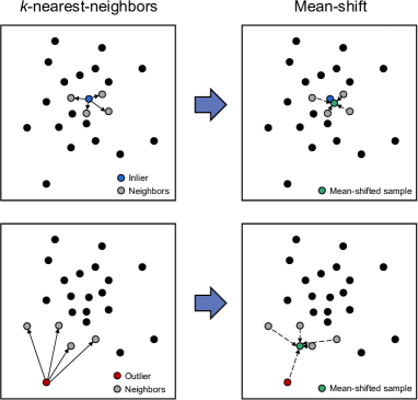
Figure 5: A 2-D illustration of the mean-shift with $m=1$ and $k=4$ for an inlier (top) and an outlier (bottom).

The process of the mean-shift could be described as follows. Given a dataset $\mathbf{X}=\{\mathbf{x}_{1},\mathbf{x}_{2},\cdots,\mathbf{x}_{N}\}$, mean-shift first calculated each sample’s $k$-nearest-neighbors in $\mathbf{X}$. For example, for the sample $\mathbf{x}_{i}$, its $k$-nearest-neighbors set was $\text{NL}_{i}=\{\mathbf{x}_{i}^{1},\mathbf{x}_{i}^{2},\cdots,\mathbf{x}_{i}^{k}\}$. Mean-shift then added the sample itself to the neighboring set $\text{NL}_{i}=\{\mathbf{x}_{i},\mathbf{x}_{i}^{1},\mathbf{x}_{i}^{2},\cdots,\mathbf{x}_{i}^{k}\}$ and calculated the mean value of the list, as expressed in Eq. 12.

$$\left\{\begin{aligned} &\mathbf{x}_{i}^{{\rm MS}(1,k)}=\frac{1}{|\text{NL}_{i}|}\sum_{\mathbf{x}\in\text{NL}_{i}}{\mathbf{x}},\\ &\mathbf{X}^{{\rm MS}(1,k)}=\{\mathbf{x}_{1}^{{\rm MS}(1,k)},\mathbf{x}_{2}^{{\rm MS}(1,k)},\cdots,\mathbf{x}_{N}^{{\rm MS}(1,k)}\}.\end{aligned}\right.$$ (12)

Yang et al. [22] proposed to repeat the above process several times to get a better OD result. For example, the same process could be applied to $\mathbf{X}^{{\rm MS}(1,k)}$ to get $\mathbf{X}^{{\rm MS}(2,k)}$, in which ${\rm MS}(m,k)$ denotes the process of mean-shift with $k$ neighbors and $m$ shift times. A 2-D illustration of mean-shift is shown in Fig. 5.

To apply the mean-shift on the AE-based OD method, the following procedure was proposed: the AE could be trained using the loss function Eq. 9 or Eq. 10 during the training phase. During the scoring phase, the outlier score of a test sample $\mathbf{x}$ could be computed using the score function as illustrated in Eq. 13 and Eq. 14.

$$\text{MSS-MSE}(\mathbf{x})=||\mathbf{x}^{{\rm MS}(m,k)}-\hat{\mathbf{x}}||_{2}^{2},$$ (13)

$$\text{or},$$

$$\text{MSS-APRE}(\mathbf{x})=\alpha\sum_{d=1}^{D}{\frac{(x_{d}^{{\rm MS}(m,k)}-\mu_{d})^{2}}{\sigma_{d}}}+\beta\sum_{d=1}^{D}{\ln\sigma_{d}},$$ (14)

where $\mathbf{x}^{{\rm MS}(m,k)}$ denotes the mean-shifted result of the test sample $\mathbf{x}$.

 

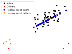
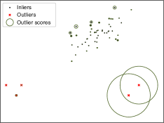
(a) Original data                     (b) Outlier scores computed

and data reconstructed by AE.                          by MSE.

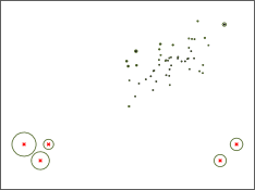
(c) Outlier scores computed by MSS-MSE with $m=1,k=6$

.

Figure 6: A 2-D example of the effect of the MSS. The original data was identical to Fig. 4. Then, an AE was trained using these data with the loss function of MSE. (b) and (c) showed the outlier scores generated by MSE and MSS-MSE with $m=1,k=6$ respectively. The larger the radius of the green circle, the higher the outlier score.

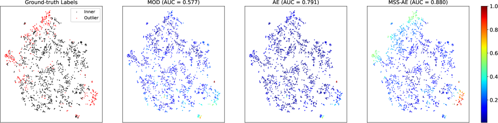
(a)                                   (b)                                   (c)                                    (d)

Figure 7: An illustration of the MSS method on the Cardiotocography dataset. The data in Cardiotocography were dimension-reduced to 2-D utilizing t-SNE. (a) showed the ground-truth label map of the data, in which the black points denote the inliers and the red points denote the outliers. (b)(c) and (d) showed the outlier score map generated by MOD, AE, and MSS-AE respectively.

This concept might be analyzed from two perspectives. Upon analysis of the distance measurement, the reconstruction error could be viewed as the deviation of the object’s position in the original data space. The reconstruction error of the inlier was relatively small if AE was well-trained, which means the reconstructed inlier lies within close proximity to the original position. Meanwhile, the mean-shifted result of an inlier was also close to its original position, hence the distance between the reconstructed inlier and the mean-shifted inlier would be small. For the outliers, the mean-shifted result was generally closer to inliers and further from its original locality. The outliers’ reconstruction result deviated in a larger magnitude for distance, and with a random direction, since AE learning was inadequate. Thus, the distance between an outlier’s mean-shifted result and reconstruction result would be especially large compared to an inlier, which made them simple to distinguish. Upon analysis of the reconstruction probability, even though an outlier was reconstructed with a relatively high probability, its mean-shifted result was not similar to the reconstruction. This resulted in a high outlier score as the mean-shifted result fell into the position with low probability within the probability distribution.

In theory, usage of the distance between the mean of $k$-NN instead of the original data and the reconstructed data had two benefits. First, some data shared common mean values, hence similar data in the feature space could have similar outlier scores [57]. Therefore, it avoided local variance in outlier score space. Second, the mean values were seen as the representatives of $k$-NN, thus it considered both object-level and group-level factors when scoring [58]. Therefore, it provided a robust method for the detection of both point outliers and collective outliers.

An example of the effect of the MSS is shown in Fig. 6. The reconstruction errors of the outliers lying on the bottom left were small, making identification of these outliers from inliers challenging. However, they were easily identified after applying the MSS with $m=1$ and $k=6$.

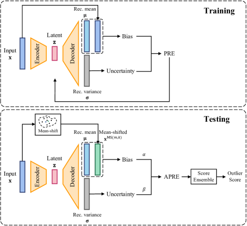
Figure 8: An illustration of the training and testing procedure of MSS-PAE. “Rec.” in the figure denotes “Reconstruction”.

Fig. 7 demonstrates an example of the MSS method on the Cardiotocography dataset. In this case, the MSS was applied to the conventional AE, termed MSS-AE. For better presentation, the data in Cardiotocography were dimension-reduced to 2-D utilizing t-distributed stochastic neighbor embedding (t-SNE) [59]. Fig. 7. (a) shows the ground-truth label map of the data, where the black points denote the inliers and the red points denote the outliers. The outliers were observed to be distributed in the top left region and bottom right region of the map. Figs. 7. (b), (c), and (d) illustrate the outlier score map generated by MOD, AE, and MSS-AE respectively. The color scale corresponds to the outlier score of each object. The performance is evaluated by the Area Under Curve (AUC) of Receiver Operating Characteristic (ROC). MOD was observed to excel at distinguishing outliers at the bottom right of the map, but was unable to distinguish outliers at the top left and had poor accuracy for inliers. The inadequacies were reflected by its abysmal AUC of 0.577. AE could distinguish the part of the outliers lying at the bottom right and achieve a better AUC of 0.791, but could not distinguish the outliers at the top left either. The outlier scores were also not differentiable enough. In contrast, MSS-AE could distinguish both outliers lying at the bottom right and top left. MSS-AE provided more differentiable outlier scores and a significant improvement in AUC performance to 0.880.

The MSS could also be applied to the PAE proposed in Sec. III-A, producing MSS-PAE. An illustration of the training and testing procedure of MSS-PAE was shown in Fig. 8. The performance of MSS-PAE was evaluated in the Sec. IV.

III-C Practical implementation

In order to bring the proposed methods from theory to practice, several processing tricks were necessary to apply. Thus, the salient practical implementation details are introduced in this section, including the semi-supervised model evaluation and AEs score ensemble. Finally, a two-step procedure for the MSS is summarized.

III-C1 Semi-supervised model evaluation

Although the AE training was unsupervised, the optimal stopping point of the training procedure was hard to determine since contamination of training set by outliers would result in AE adapting and reconstructing outliers with the further iterations of training [60, 51, 45]. This challenge remains a scope for further study. In this study, a semi-supervised training method was adopted to avoid the issue.

Specifically, the data were divided into three sets: training set, validation set, and test set. All three sets contained similar proportions of inliers and outliers, but only the validation set contained the corresponding ground-truth label (0 for inliers and 1 for outliers). Then, the training set was used to train the AE, the validation set was used to pick the optimal stopping points and hyper-parameters, and the test set was used to report the final result.

For the proposed MSS method, all samples’ mean-shifted results were computed in advance. The result of mean-shifting depended on the visible dataset and the hyper-parameter $k$, which denotes the number of the nearest neighbors used in the mean-shift computation. In addition, $k$ was sensitive to the scale of the dataset, hence the computation for mean-shifting is different for different sets. For the training set, the mean-shifted result could be directly computed. For the validation and test set, each sample was added to the training set then computing the mean-shifted result, to simulate the practical scenario. To reduce the computational complexity, a $k$-d tree was built [61] based on the training set. Then, for a test sample, it was inserted into the $k$-d tree as a leaf node and its $k$-nearest-neighbors could be obtained following the tree algorithms. The building and searching time complexity were $O(\log N)$ and $O(k\log N)$ respectively.

III-C2 Autoencoders score ensemble

The instability of the optimization of the AE-based method was a problem. With insufficient training data, the optimization could easily terminate at a local optimum, producing poor results. In this case, the direction of the gradient descent relied on the initial state of AE. Ishii et al. [50] generated 20 initial states for AE and computed the average AUC as the evaluation result. This approach reflected nearly the true performance of the model, but it might not be practical as it did not give the final outlier scores explicitly. In this study, the final score was reported in a format of the score ensemble. Specifically, $S$ initial states were generated for AEs and trained separately. After training, $S$ trained models were applied to the validation set and their performances were computed via AUC to find the best $S_{b}$ models. The best models were used as the final detectors. Finally, the test sample was delivered to the aforementioned detectors to produce $S_{b}$ scores. The scores were then normalized and an average score was computed as the ensemble result, i.e.,

$${\rm score}=\frac{1}{S_{b}}\sum_{i=1}^{S_{b}}{\frac{{\rm score}_{i}-b}{a-b}},$$ (15)

where ${\rm score}_{i}$ denotes the score of the $i$-th AE, $a$ and $b$ are two scaling factors, and ${\rm score}$ denotes the final ensemble score.

III-C3 A two-step procedure

The MSS for AE consisted of two steps. The first step was to find the optimal number of nearest neighbors used in the mean-shift, i.e. $k$, which was a critical hyper-parameter in the proposed method, and relied on the structure and scale of the specific dataset. To calculate this, a candidate list of $k$ was evaluated at each epoch of the AE training using the AUC metric with the validation set. The best AUC for each $k$ was recorded. Repeating the above training procedure using $S_{1}$ initial states, $S_{1}$ AUC results for each $k$ were obtained. The average of the $S_{1}$ AUC results was calculated, and the $k$ with the best average AUC was selected as the optimal $k$.

The second step was to obtain the final ensemble outlier scores. $S_{2}$ initial states were generated to train the AEs. It is worth noting that $S_{1}$ was smaller to reduce the time complexity of computing the optimal $k$, and $S_{2}$ was larger to improve the final ensemble performance and stability. At each training epoch, the outlier scores of the validation dataset were computed with the optimal $k$, and the AUC performance was evaluated. The model with the best AUC over all epochs was recorded for each initial state. Then, the outlier scores of the test data were computed using the top $S_{b}$ models and integrated via Eq. 15.

IV Experiments

To show the effectiveness of the proposed methods, experiments were conducted on 32 commonly used real-world outlier detection datasets. The proposed methods were compared with 5 typical AE-based OD methods (including AE itself), and proved the efficacy of applying the MSS. A comparison was made against 5 classic non-AE-based SOTA OD methods.

The experiments answered the following questions:

1) How effective and flexible is the APRE? (Sec. IV-C1)

2) How do hyper-parameters $k$ and $m$ affect the MSS? (Sec. IV-C2)

3) Is the MSS beneficial for other AE-based methods? (Sec. IV-C3)

4) Comparing the proposed methods with 5 AE-based and 5 non-AE-based OD methods, which one yields the best performance? (Sec. IV-C3 and Sec. IV-C4)

TABLE II: Information of 32 real-world outlier detection datasets.

Name	Dimension	Instances	Outliers	Ratio
ALOI	27	49,534	1,508	3.0%
Annthyroid	21	7,129	534	7.5%
Arrhythmia	259	450	206	45.8%
Breastw	9	683	239	35.0%
Cardiotocography	21	2,114	466	22.0%
Glass	7	214	9	4.2%
HeartDisease	13	270	120	44.4%
InternetAds	1,555	1,966	368	18.7%
Ionosphere	32	351	126	35.9%
Letter	32	1,600	100	6.3%
Lymphography	3	148	6	4.1%
Mammography	6	11,183	260	2.3%
Mnist	100	7,603	700	9.2%
Musk	166	3,062	97	3.2%
Optdigits	64	5,216	150	2.9%
PageBlocks	10	5,393	510	9.5%
Parkinson	22	195	147	75.4%
PenDigits	16	9,868	20	0.2%
Pima	8	768	268	34.9%
Satellite	36	6,435	2,036	31.6%
Satimage-2	36	5,803	71	1.2%
Shuttle	9	1,013	13	1.3%
SpamBase	57	4,207	1,679	39.9%
Speech	400	3,686	61	1.7%
Stamps	9	340	31	9.1%
Thyroid	6	3,772	93	2.5%
Vertebral	6	240	30	12.5%
Vowels	12	1,456	50	3.4%
Waveform	21	3,443	100	2.9%
Wilt	5	4,819	257	5.3%
Wine	13	129	10	7.8%
WPBC	33	198	47	23.7%

TABLE III: Architecture setting of the AE-based methods.

Dimsension (D)	Number of layers	Number of units
<20	3	[D, D // 2, D]
$\geq$20, <100	5	[D, D // 2, D // 4, D // 2, D]
$\geq$100, <200	7	[D, D // 2, D // 4, D // 8, D // 4, D // 2, D]
$\geq$200	7	[D, D // 2, D // 4, D // 16, D // 4, D // 2, D]

TABLE IV: AUC results of AE and PAE with different {$\alpha$,$\beta$}.

Dataset	AE[35]	PAE*
		$\alpha=0.5,\beta=2$	$\alpha=0.5,\beta=1$	$\alpha=1,\beta=1$	$\alpha=1,\beta=0.5$	$\alpha=2,\beta=0.5$
ALOI	0.563	0.545	0.559	0.562	0.556	0.564
Annthyroid	0.608	0.799	0.793	0.790	0.850	0.835
Arrhythmia	0.714	0.736	0.740	0.624	0.706	0.649
Breastw	0.972	0.994	0.995	0.994	0.971	0.971
Cardiotocography	0.811	0.818	0.818	0.819	0.858	0.870
Glass	0.804	0.961	0.980	0.873	0.912	0.882
HeartDisease	0.813	0.865	0.871	0.859	0.831	0.768
InternetAds	0.706	0.685	0.681	0.671	0.674	0.697
Ionosphere	0.971	0.985	0.971	0.914	0.957	0.956
Letter	0.857	0.855	0.768	0.808	0.764	0.807
Lymphography	0.971	0.914	0.914	0.914	0.914	0.914
Mammography	0.893	0.884	0.882	0.891	0.877	0.874
Mnist	0.882	0.948	0.945	0.931	0.906	0.891
Musk	1.000	1.000	1.000	1.000	1.000	1.000
Optdigits	0.760	0.936	0.912	0.865	0.850	0.874
PageBlocks	0.952	0.962	0.946	0.949	0.942	0.953
Parkinson	0.627	0.815	0.662	0.711	0.611	0.576
PenDigits	0.879	0.951	0.929	0.913	0.897	0.907
Pima	0.651	0.756	0.736	0.698	0.696	0.683
Satellite	0.750	0.855	0.845	0.817	0.777	0.740
Satimage-2	0.993	0.983	0.983	0.988	0.988	0.988
Shuttle	0.995	0.996	0.988	0.992	0.992	0.992
SpamBase	0.565	0.847	0.793	0.712	0.646	0.650
Speech	0.551	0.541	0.532	0.561	0.597	0.495
Stamps	0.931	0.844	0.952	0.950	0.948	0.948
Thyroid	0.975	0.973	0.991	0.977	0.979	0.982
Vertebral	0.607	0.676	0.772	0.349	0.747	0.758
Vowels	0.937	0.968	0.976	0.972	0.955	0.931
Waveform	0.781	0.881	0.790	0.776	0.771	0.771
Wilt	0.383	0.822	0.823	0.818	0.861	0.879
Wine	0.914	0.879	0.897	0.897	0.914	0.914
WPBC	0.499	0.548	0.516	0.501	0.484	0.479
AVG.	0.791(7)	0.851(13)	0.843(9)	0.815(1)	0.826(3)	0.819(5)

• a. The number in parentheses in the AVG. row denotes the number of datasets on which the method achieves the best performance.

• b. * denotes the proposed method.

IV-A Datasets and baselines

32 real-world outlier detection datasets were obtained from DAMI and ODDS dataset repositories. The summary of these datasets was shown in TABLE II. We divided each dataset into the training set and test set with a ratio of 3:1. Then, one-third of the samples in the training set were selected to form the validation set. The outlier ratios were kept constant in all three sets, and the validation set and test set included the data labels but the training set did not. In addition, each attribute of the data was normalized to zero-mean and unit-variance using the Mean-SD normalization [62]. The mean value and the standard deviation value were obtained from the training set. This operation was essential for the AE-based methods because it balanced the scale of each attribute of the data, lest the attributes with relatively large scale of values had unexpectedly bigger impacts on the model optimization.

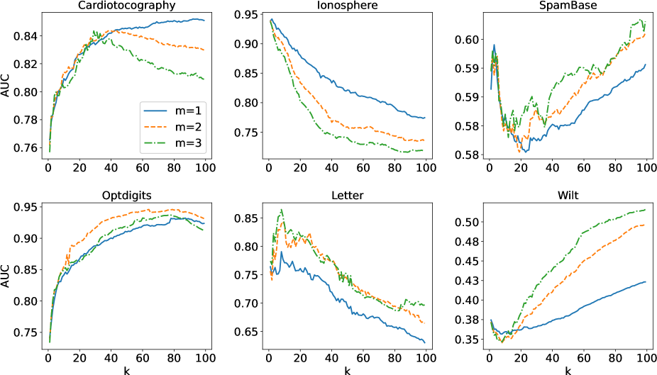
Figure 9: The performance curves as $k$ was increased from 1 to 99 on 6 datasets (Cardiotocography, Ionosphere, SpameBase, Optdigits, Letter and Wilt). Each individual graph has three curves with different $m$ denoting the time of mean-shifting. For each dataset, the $k$-NN relationships were computed on the corresponding training set ($\frac{3}{4}$ size of the complete set) and the AUC results were evaluated on the corresponding validation set.

To show the superiority of the proposed methods, 5 typical AE-based methods and 5 classic SOTA OD methods were used as the baselines. The 5 typical AE-based methods were AE [35], RDA [36], LCAE [50], RSRAE [52] and FDAE [39]. The details of these methods were introduced in Sec. II-B. The 5 classic non-AE-based SOTA OD methods were proximity-based Local Outlier Factor (LOF) [18], classification-based One-Class Support Vector Machines (OCSVM) [26], ensemble-based Isolation Forest (iForest) [29], probabilistic-based Empirical-Cumulative-distribution-based Outlier Detection (ECOD) [34] and MOD [22]. The AE-based methods were reproduced, compared to their original results, and the proposed MSS method was applied to improve the performance. All the methods were implemented using Python, and the implementation from PyOD [63] toolkit with default hyper-parameters found in literature was used for non-AE-based methods. AUC was used as the evaluation metric.

IV-B Experimental setup

The architecture of PAE had been introduced in Sec. III-A. The model used PRE as the training loss function and APRE as the scoring function. The MSS is a universal scoring method that can be applied to most AE-based methods including the proposed PAE. As notations, application to AE produced MSS-AE and application to RSRAE produced MSS-RSRAE, and so on.

TABLE V: AUC results of AE vs. MSS-AE, PAE vs. MSS-PAE and MOD.

Dataset	AE[35]	MSS-AE*			PAE*	MSS-PAE*			MOD[22]
		$m=1$	$m=2$	$m=3$		$m=1$	$m=2$	$m=3$	$m=1$	$m=2$	$m=3$
ALOI	0.563	0.558	0.563	0.561	0.545	0.630	0.658	0.664	0.769	0.751	0.738
Annthyroid	0.608	0.603	0.630	0.641	0.799	0.856	0.886	0.893	0.716	0.712	0.704
Arrhythmia	0.714	0.720	0.724	0.730	0.736	0.716	0.761	0.762	0.711	0.715	0.718
Breastw	0.972	0.994	0.987	0.987	0.994	0.994	0.996	0.992	0.985	0.980	0.987
Cardiotocography	0.811	0.875	0.888	0.877	0.818	0.841	0.844	0.844	0.584	0.591	0.598
Glass	0.804	0.922	0.863	0.951	0.961	0.804	0.824	0.843	0.941	0.931	0.941
HeartDisease	0.813	0.859	0.869	0.799	0.865	0.892	0.883	0.886	0.726	0.745	0.758
InternetAds	0.706	0.724	0.801	0.783	0.685	0.797	0.797	0.797	0.660	0.621	0.619
Ionosphere	0.971	0.978	0.975	0.973	0.985	0.962	0.964	0.962	0.932	0.927	0.926
Letter	0.857	0.844	0.860	0.853	0.855	0.748	0.742	0.798	0.893	0.905	0.890
Lymphography	0.971	1.000	1.000	1.000	0.914	0.971	1.000	1.000	1.000	1.000	1.000
Mammography	0.893	0.876	0.885	0.885	0.884	0.882	0.885	0.882	0.844	0.838	0.832
Mnist	0.882	0.876	0.881	0.882	0.948	0.949	0.949	0.948	0.860	0.859	0.855
Musk	1.000	1.000	1.000	1.000	1.000	1.000	1.000	1.000	0.991	0.990	0.997
Optdigits	0.760	0.957	0.970	0.981	0.936	0.994	0.993	0.992	0.494	0.430	0.414
PageBlocks	0.952	0.955	0.948	0.953	0.962	0.958	0.957	0.954	0.921	0.920	0.914
Parkinson	0.627	0.639	0.769	0.736	0.815	0.766	0.796	0.819	0.606	0.641	0.669
PenDigits	0.879	0.887	0.974	0.973	0.951	0.963	0.977	0.971	0.948	0.971	0.976
Pima	0.651	0.689	0.691	0.699	0.756	0.757	0.740	0.722	0.606	0.625	0.634
Satellite	0.750	0.788	0.789	0.763	0.855	0.856	0.857	0.857	0.695	0.677	0.671
Satimage-2	0.993	0.993	0.991	0.989	0.983	0.981	0.975	0.967	0.996	0.996	0.998
Shuttle	0.995	0.997	1.000	0.997	0.996	1.000	0.997	0.997	0.989	0.989	0.989
SpamBase	0.565	0.580	0.622	0.623	0.847	0.886	0.879	0.878	0.530	0.532	0.538
Speech	0.551	0.567	0.586	0.651	0.541	0.658	0.477	0.527	0.734	0.700	0.721
Stamps	0.931	0.961	0.915	0.950	0.844	0.954	0.942	0.837	0.935	0.937	0.935
Thyroid	0.975	0.972	0.963	0.960	0.973	0.994	0.991	0.990	0.955	0.960	0.963
Vertebral	0.607	0.755	0.750	0.745	0.676	0.687	0.712	0.703	0.533	0.536	0.522
Vowels	0.937	0.906	0.925	0.958	0.968	0.945	0.940	0.943	0.931	0.984	0.981
Waveform	0.781	0.792	0.826	0.872	0.881	0.895	0.897	0.901	0.713	0.734	0.700
Wilt	0.383	0.427	0.478	0.511	0.822	0.884	0.873	0.676	0.667	0.621	0.622
Wine	0.914	0.948	1.000	1.000	0.879	0.948	0.966	0.966	0.931	0.931	0.914
WPBC	0.499	0.506	0.413	0.477	0.548	0.415	0.428	0.450	0.491	0.489	0.509
AVG.	0.791(6)	0.817(9)	0.829(11)	0.836(14)	0.851(8)	0.862(11)	0.862(12)	0.857(12)	0.790(16)	0.789(8)	0.788(14)

TABLE VI: AUC results of 6 AE-based methods and their MSS- versions.

Dataset	AE	MSS-AE	PAE	MSS-PAE	RDA	MSS-RDA	LCAE	MSS-LCAE	RSRAE	MSS-RSRAE	FDAE	MSS-FDAE
	[35]	*	*	*	[36]	*	[50]	*	[52]	*	[39]	*
ALOI	0.563	0.563	0.564	0.706	0.562	0.557	0.553	0.584	0.549	0.571	0.547	0.540
Annthyroid	0.608	0.641	0.850	0.893	0.608	0.617	0.749	0.689	0.611	0.606	0.623	0.617
Arrhythmia	0.714	0.730	0.740	0.762	0.714	0.729	0.724	0.713	0.711	0.724	0.709	0.639
Breastw	0.972	0.994	0.995	0.996	0.972	0.995	0.988	0.993	0.995	0.996	0.993	0.989
Cardiotocography	0.811	0.888	0.870	0.899	0.811	0.888	0.812	0.883	0.812	0.901	0.812	0.901
Glass	0.804	0.951	0.980	0.853	0.863	0.980	0.922	0.863	0.745	0.941	0.755	0.951
HeartDisease	0.813	0.869	0.871	0.905	0.813	0.885	0.770	0.909	0.799	0.845	0.750	0.848
InternetAds	0.706	0.801	0.697	0.839	0.707	0.801	0.702	0.765	0.653	0.754	0.665	0.711
Ionosphere	0.971	0.978	0.985	0.978	0.968	0.968	0.980	0.977	0.965	0.962	0.949	0.952
Letter	0.857	0.860	0.855	0.798	0.820	0.833	0.855	0.832	0.867	0.794	0.829	0.793
Lymphography	0.971	1.000	0.914	1.000	0.971	1.000	0.971	1.000	1.000	1.000	1.000	1.000
Mammography	0.893	0.885	0.891	0.901	0.892	0.890	0.896	0.895	0.907	0.907	0.890	0.890
Mnist	0.882	0.882	0.948	0.949	0.882	0.889	0.925	0.919	0.891	0.886	0.892	0.882
Musk	1.000	1.000	1.000	1.000	1.000	1.000	1.000	1.000	1.000	1.000	1.000	1.000
Optdigits	0.760	0.981	0.936	0.995	0.760	0.981	0.759	0.950	0.795	0.998	0.818	0.990
PageBlocks	0.952	0.955	0.962	0.958	0.952	0.956	0.944	0.948	0.959	0.961	0.958	0.961
Parkinson	0.627	0.769	0.815	0.861	0.620	0.769	0.755	0.725	0.690	0.778	0.653	0.764
PenDigits	0.879	0.974	0.951	0.993	0.841	0.970	0.925	0.976	0.764	0.946	0.831	0.960
Pima	0.651	0.699	0.756	0.757	0.651	0.693	0.677	0.677	0.681	0.723	0.661	0.667
Satellite	0.750	0.789	0.855	0.857	0.745	0.791	0.830	0.858	0.817	0.829	0.840	0.847
Satimage-2	0.993	0.993	0.988	0.987	0.993	0.993	0.994	0.993	0.992	0.990	0.993	0.978
Shuttle	0.995	1.000	0.996	1.000	0.995	0.997	0.960	1.000	0.989	1.000	0.977	0.987
SpamBase	0.565	0.623	0.847	0.886	0.554	0.623	0.548	0.734	0.594	0.771	0.570	0.716
Speech	0.551	0.651	0.597	0.673	0.525	0.651	0.529	0.634	0.507	0.528	0.563	0.488
Stamps	0.931	0.961	0.952	0.954	0.957	0.961	0.941	0.974	0.941	0.957	0.941	0.918
Thyroid	0.975	0.972	0.991	0.994	0.976	0.972	0.980	0.980	0.982	0.982	0.971	0.970
Vertebral	0.607	0.755	0.772	0.841	0.593	0.755	0.676	0.808	0.602	0.745	0.703	0.695
Vowels	0.937	0.958	0.976	0.945	0.925	0.939	0.919	0.929	0.901	0.886	0.727	0.707
Waveform	0.781	0.872	0.881	0.901	0.781	0.817	0.834	0.758	0.783	0.859	0.802	0.812
Wilt	0.383	0.511	0.879	0.891	0.388	0.503	0.483	0.559	0.529	0.529	0.529	0.536
Wine	0.914	1.000	0.914	1.000	0.914	1.000	0.897	0.983	0.914	1.000	0.966	1.000
WPBC	0.499	0.506	0.548	0.484	0.499	0.506	0.526	0.575	0.612	0.521	0.585	0.764
AVG.	0.791(1)	0.844(4)	0.868(4)	0.889(19)	0.789(1)	0.841(4)	0.813(2)	0.846(6)	0.799(4)	0.840(9)	0.797(2)	0.827(6)

TABLE VII: AUC results of the proposed methods and SOTA baselines.

Dataset	ECOD[34]	iForest[29]	LOF[18]	OCSVM[26]	MOD[22]	AE[35]	PAE*	MSS-AE*	MSS-PAE*
ALOI	0.540	0.544	0.768	0.540	0.769	0.563	0.564	0.563	0.706
Annthyroid	0.739	0.652	0.677	0.600	0.716	0.608	0.850	0.641	0.893
Arrhythmia	0.732	0.740	0.712	0.706	0.718	0.714	0.740	0.730	0.762
Breastw	0.992	0.989	0.417	0.949	0.987	0.972	0.995	0.994	0.996
Cardiotocography	0.802	0.706	0.545	0.718	0.598	0.811	0.870	0.888	0.899
Glass	0.853	0.922	0.637	0.882	0.941	0.804	0.980	0.951	0.853
HeartDisease	0.687	0.721	0.667	0.696	0.758	0.813	0.871	0.869	0.905
InternetAds	0.722	0.764	0.606	0.653	0.660	0.706	0.697	0.801	0.839
Ionosphere	0.789	0.895	0.862	0.885	0.932	0.971	0.985	0.978	0.978
Letter	0.549	0.575	0.846	0.566	0.905	0.857	0.855	0.860	0.798
Lymphography	1.000	1.000	0.857	1.000	1.000	0.971	0.914	1.000	1.000
Mammography	0.914	0.864	0.718	0.873	0.844	0.893	0.891	0.885	0.901
Mnist	0.751	0.819	0.724	0.855	0.860	0.882	0.948	0.882	0.949
Musk	0.967	1.000	0.716	1.000	0.997	1.000	1.000	1.000	1.000
Optdigits	0.615	0.799	0.527	0.511	0.494	0.760	0.936	0.981	0.995
PageBlocks	0.914	0.905	0.676	0.917	0.921	0.952	0.962	0.955	0.958
Parkinson	0.350	0.414	0.380	0.382	0.669	0.627	0.815	0.769	0.861
PenDigits	0.392	0.758	0.907	0.366	0.976	0.879	0.951	0.974	0.993
Pima	0.537	0.592	0.567	0.578	0.634	0.651	0.756	0.699	0.757
Satellite	0.608	0.724	0.534	0.694	0.695	0.750	0.855	0.789	0.857
Satimage-2	0.969	0.992	0.507	0.996	0.998	0.993	0.988	0.993	0.987
Shuttle	0.723	0.820	0.992	0.949	0.989	0.995	0.996	1.000	1.000
SpamBase	0.679	0.622	0.437	0.524	0.538	0.565	0.847	0.623	0.886
Speech	0.507	0.527	0.524	0.504	0.734	0.551	0.597	0.651	0.673
Stamps	0.870	0.931	0.720	0.887	0.937	0.931	0.952	0.961	0.954
Thyroid	0.977	0.977	0.685	0.956	0.963	0.975	0.991	0.972	0.994
Vertebral	0.596	0.552	0.552	0.555	0.536	0.607	0.772	0.755	0.841
Vowels	0.632	0.767	0.962	0.792	0.984	0.937	0.976	0.958	0.945
Waveform	0.674	0.759	0.752	0.738	0.734	0.781	0.881	0.872	0.901
Wilt	0.350	0.437	0.654	0.281	0.667	0.383	0.879	0.511	0.891
Wine	0.897	0.862	0.879	0.741	0.931	0.914	0.914	1.000	1.000
WPBC	0.482	0.479	0.514	0.509	0.509	0.499	0.548	0.506	0.484
AVG.	0.713(2)	0.753(2)	0.672(0)	0.713(2)	0.800(6)	0.791(1)	0.868(5)	0.844(4)	0.889(22)

Considering all the data were tabular data, fully-connected layers were used to construct the AE. The number of the layers depended on the dimension of the input data. The detailed setting of the network architecture was shown in TABLE III. Then, the rectified linear unit (ReLU) activation was added after each layer of the AE except the last layer to increase the nonlinearity of the network. ReLU is widely used as an activation function in deep neural networks [64]. It mimics neuronal mechanisms in the human brain, and demonstrated good performance in many tasks while requiring only a few computational resources. The settings were applied to all the AE-based methods in this experiment. Additionally, the settings of different methods’ individual hyper-parameters were established as such: the percentile value in LCAE was set to 70; the size of the RSR layer in RSRAE and FDAE was set to half of the latent layer’s size. For RDA, the number of inner training epochs was set to 500 and the number of outer training epochs was set to 10. For other AE-based methods, the number of training epochs was set to 5,000. All these methods were optimized using the Adam optimizer [65] with a learning rate of 0.001.

The proposed methods had certain unique settings. Firstly, the variance estimated by PAE should be positive, hence a Softplus action was added after the variance output. Secondly, there were two scaling hyper-parameters in APRE. Five distinct groups were tested: {$\alpha=0.5,\beta=2$}, {$\alpha=0.5,\beta=1$}, {$\alpha=1,\beta=1$}, {$\alpha=1,\beta=0.5$} and {$\alpha=2,\beta=0.5$}. The results are shown in Sec. IV-C1. Thirdly, similar to MOD, the mean-shift time $m$ also affected the performance of the MSS significantly. The value of $m$ was varied from 1 to 3, and the performance was reported in Sec. IV-C2. Fourthly, the number of nearest neighbors $k$ was also an essential parameter for MSS. We proposed selecting the optimal $k$ from a candidate list $\mathbf{k}$. In our experiments, $\mathbf{k}=[1,2,\cdots,\min(99,N-1)]$, where $N$ denotes the number of the instances in the training set. Lastly, for the two-step procedure mentioned in Sec. III-C3, $S_{1}=20$ for the first step, $S_{2}=20$ and $S_{b}=5$ for the second step. The code is available on www.OutlierNet.com for reproducibility.

IV-C Experimental results

IV-C1 Evaluation of the probabilistic autoencoder

In this section, the performance of PAE was evaluated. As shown in TABLE IV, the average performance over 32 real-world datasets of PAE with all five groups of {$\alpha$, $\beta$} was better than the general AE. The largest relative improvement of the average AUC was 29% (0.851 vs. 0.791), comparing PAE ($\alpha=0.5$, $\beta=2$) and AE. Moreover, PAE significantly outperformed AE on some datasets, such as Annothyroid (0.850 vs. 0.608), Glass (0.980 vs. 0.804), Optdigits (0.936 vs. 0.760), SpamBase (0.847 vs. 0.565) and Wilt (0.879 vs. 0.383), which showed its superiority for specific applications.

The optimal values of $\alpha$ and $\beta$ were application-dependent. For example, on dataset ALOI, Cardiotocography, Wilt and Wine, the performance improved as $\alpha$ increased, which implied that the bias term was more critical in these applications. In contrast, for datasets on dataset Optdigits, PenDigits, Satellite and Waveform, the performance improved as $\beta$ increased, which implied that the uncertainty term was more critical in these applications. The logical deduction was that a suitable group of {$\alpha$, $\beta$} should be selected based on the specific application to achieve the best OD performance.

The experiments illustrated that the average performance of all the other groups was better than the group of {$\alpha=1,\beta=1$} (which was equivalent to PRE), which proved the importance of the adjustable parameters in APRE. In addition, the group of {$\alpha=0.5,\beta=2$} achieved the best performance on 13 datasets (41%) and the best average AUC performance (0.851). This clearly demonstrated that the uncertainty of AE was critical for OD, and even more important than the commonly used bias measurement in many applications. Insufficient emphasis had been placed on this variable, and significant change could be brought about by the discovery in this experiment. This finding has potential to facilitate the AE-based methods in OD applications.

IV-C2 Evaluation of the mean-shift outlier scoring

The number of nearest neighbors $k$ and the time of mean-shifting $m$ were two important parameters for the MSS method. In reality, they were all application-dependent. The effect of $k$ was demonstrated for MSS-AE on several datasets in Fig. 9. The figure illustrated the variation in performance as $k$ was increased for different datasets, and the distinct optimal $k$ for each dataset. Similar to all the $k$-NN-based methods, this factor depended on the data structure of the specific application.

The AUC results for MSS-AE, MSS-PAE ($\alpha=0.5,\beta=2$), and MOD were listed in TABLE V. Variation of the time of mean-shifting $m=1,2,3$ was tested for all three methods, and the optimal $k$ for each case was found in the first step. The average results on 32 datasets demonstrated that MSS-AE and MSS-PAE triumphed their counterparts AE and PAE respectively. Moreover, MSS-AE and MSS-PAE also outperformed MOD, a SOTA detector. The best average AUC performance for MSS-AE was 0.836 when $m=3$, and for MSS-PAE, it was 0.858 when $m=1$, which was the best among all competitors. For a total of 32 datasets, MSS-AE was better on 27 datasets (84%) compared with AE, and MSS-PAE was better on 24 datasets (75%) compared with PAE, which proved the effectiveness of the MSS. TABLE V illustrated that, the MSS significantly improved the performance on the datasets where AE (or PAE) and MOD had poor performance, such as InternetAds, Optidigits, Speech and Vertebral. This proved that the combination of the AE-based method and the MSS was effective.

IV-C3 Comparison with other AE-based OD methods

To show the superiority of the proposed APRE function and the versatility of the MSS method, the performance of PAE, 5 AE-based OD methods, and their mean-shifted versions were compared in TABLE VI. The results of all MSS- versions were obtained with the optimal value of $m$, and the results of PAE and MSS-PAE were obtained using the best group of {$\alpha$, $\beta$}. The table conclusively showed that all MSS- versions outperformed their original counterpart with average 20% of the relative performance improvement on the average AUC, proving the versatility of the MSS method. Then among all standard versions, PAE achieved the best average AUC performance, which gained a 29% relative improvement comparing to the second best method LCAE (0.868 vs. 0.813). Among all MSS- versions, MSS-PAE also achieved the best average AUC performance, which gained a 28% relative improvement comparing to the second best method MSS-LCAE (0.889 vs. 0.846). This result suggested that the proposed APRE was effective, especially when jointly incorporated with the MSS method.

IV-C4 Comparison with non-AE-based SOTA OD methods

The relative performance of the proposed method against 5 non-AE-based SOTA OD methods were summarized in TABLE VII. The results showed that the proposed PAE, MSS-AE, and MSS-PAE outperformed all the baselines on average AUC, where MSS-PAE achieved the best performance on 22 datasets among all 32 datasets (69%) and had the best average AUC of 0.889 (45% relative improvement comparing with MOD which was the best of 5 baselines).

V Discussion

Experimental results proved the superiority of the proposed methods. As shown in TABLE IV, TABLE V and Fig. 9, the performance gained great improvement with proper hyper-parameters, including $\alpha,\beta$ for APRE and $m,k$ for the MSS. In this paper, the hyper-parameters were selected with the auxiliary of a small set of labeled data. It is worth noting that the label information was only used to validate the model performance instead of training the model directly, which made the proposed methods different from the existing semi-supervised OD methods. Besides, a limit amount of labeled data are unreachable in many practical applications [66, 28, 67].

The proposed loss function PRE and scoring function APRE demonstrated great effectiveness in OD as shown in Sec. IV-C1 and Sec. IV-C3. In this paper, they were applied to the conventional AE producing PAE. The architecture design of PAE was simple in this work but could be more delicate in future, such as using two different decoders to generate two outputs. In addition, speculatively, the two functions may be applied to improve the performance of other AE-based OD methods, even other machine learning tasks, which was not evaluated in this paper but can be experimented in the future work.

The proposed MSS method improved the performance of all AE-based OD baselines as shown in Sec. IV-C3, utilizing the $k$-NN information. But it could be less effective and efficient confronting extremely high-dimensional and large-scale data. This may be mitigated by coupling with the dimensional-reduction and sub-sampling techniques.

VI Conclusion

In this paper, we first proposed the PRE and APRE, which considers both the reconstruction bias and judgment uncertainty of AE’s result. PRE improved AE’s learning ability and APRE further promoted AE’s performance on OD tasks. We also proposed the MSS method, which increases AE’s robustness when some outliers are reconstructed well unexpectedly. The experimental results on 32 real-world OD datasets showed that the proposed methods significantly improved AE’s performance on OD. Specifically, APRE was quite effective and flexible when adapting to different OD applications, and the proposed MSS method could be effectively applied to other AE-based OD methods. Furthermore, MSS-PAE, which was the combination of the proposed two methods, performed best among all baselines. Therefore, we recommend to use the proposed APRE and MSS simultaneously to get the best performance in practice. We believe that the MSS method can be used as a general plugin for most AE-based OD methods. PRE or APRE may also be applied to improve the performance of other AE-based methods, which was not evaluated in this paper but can be validated in the future work.

References

- [1] F. E. Grubbs, “Procedures for detecting outlying observations in samples,” Technometrics, vol. 11, no. 1, pp. 1–21, 1969.
- [2] M. Goldstein and S. Uchida, “A comparative evaluation of unsupervised anomaly detection algorithms for multivariate data,” PLoS ONE, vol. 11, no. 4, p. e0152173, 2016.
- [3] U. Fiore, A. De Santis, F. Perla, P. Zanetti, and F. Palmieri, “Using generative adversarial networks for improving classification effectiveness in credit card fraud detection,” Inf. Sci., vol. 479, pp. 448–455, 2019.
- [4] S. Shehnepoor, R. Togneri, W. Liu, and M. Bennamoun, “Spatio-temporal graph representation learning for fraudster group detection,” IEEE Trans. Neural Netw. Learn. Syst., vol. Early Access, pp. 1–15, 2022.
- [5] J. Yang, S. Rahardja, and S. Rahardja, “Click fraud detection: Hk-index for feature extraction from variable-length time series of user behavior,” in Proc. of the IEEE Int. Workshop on Mach. Learn. for Signal Process. (MLSP), 2022, pp. 1–6.
- [6] S. Zhang, B. Li, J. Li, M. Zhang, and Y. Chen, “A novel anomaly detection approach for mitigating web-based attacks against clouds,” in Proc. of the IEEE Int. Conf. on Cyber Secur. and Cloud Comput. (CSCloud), 2015, pp. 289–294.
- [7] P. Ghosh, A. Losalka, and M. J. Black, “Resisting adversarial attacks using gaussian mixture variational autoencoders,” in Proc. of the AAAI Conf. Artif. Intell., vol. 33, no. 01, 2019, pp. 541–548.
- [8] W.-K. Wong, A. W. Moore, G. F. Cooper, and M. M. Wagner, “Bayesian network anomaly pattern detection for disease outbreaks,” in Proc. of the Int. Conf. on Mach. Learn. (ICML), 2003, pp. 808–815.
- [9] T. Schlegl, P. Seeböck, S. M. Waldstein, U. Schmidt-Erfurth, and G. Langs, “Unsupervised anomaly detection with generative adversarial networks to guide marker discovery,” in Proc. of the Int. Conf. on Inf. Process. in Med. Imaging (IPMI), 2017, pp. 146–157.
- [10] J. Yang, G. I. Choudhary, S. Rahardja, and P. Franti, “Classification of interbeat interval time-series using attention entropy,” IEEE Trans. Affect. Comput., vol. 14, no. 1, pp. 321–330, 2023.
- [11] S. Wang, Y. Zeng, Q. Liu, C. Zhu, E. Zhu, and J. Yin, “Detecting abnormality without knowing normality: A two-stage approach for unsupervised video abnormal event detection,” in Proc. of the ACM Int. Conf. on Multimedia (MM), 2018, pp. 636–644.
- [12] N. Li and F. Chang, “Video anomaly detection and localization via multivariate gaussian fully convolution adversarial autoencoder,” Neurocomputing, vol. 369, pp. 92–105, 2019.
- [13] X. Wang, Z. Che, B. Jiang, N. Xiao, K. Yang, J. Tang, J. Ye, J. Wang, and Q. Qi, “Robust unsupervised video anomaly detection by multipath frame prediction,” IEEE Trans. Neural Netw. Learn. Syst., vol. 33, no. 6, pp. 2301–2312, 2022.
- [14] D. Zhang, N. Li, Z.-H. Zhou, C. Chen, L. Sun, and S. Li, “ibat: detecting anomalous taxi trajectories from gps traces,” in Proc. of the Int. Conf. on Ubiquitous Comput. (UbiComp), 2011, pp. 99–108.
- [15] J. Yang, R. Mariescu-Istodor, and P. Fränti, “Three rapid methods for averaging gps segments,” Appl. Sci., vol. 9, no. 22, p. 4899, 2019.
- [16] J. Yang, X. Tan, and S. Rahardja, “Mipo: How to detect trajectory outliers with tabular outlier detectors,” Remote Sens., vol. 14, no. 21, p. 5394, 2022.
- [17] S. Ramaswamy, R. Rastogi, and K. Shim, “Efficient algorithms for mining outliers from large data sets,” in Proc. of the ACM SIGMOD Int. Conf. on Management of Data, 2000, pp. 427–438.
- [18] M. M. Breunig, H.-P. Kriegel, R. T. Ng, and J. Sander, “Lof: identifying density-based local outliers,” in Proc. of the ACM SIGMOD Int. Conf. on Management of Data, 2000, pp. 93–104.
- [19] J. Tang, Z. Chen, A. W.-C. Fu, and D. W. Cheung, “Enhancing effectiveness of outlier detections for low density patterns,” in Proc. of the Pacific-Asia Conf. on Knowl. Discov. and Data Mining (PAKDD), 2002, pp. 535–548.
- [20] Z. He, X. Xu, and S. Deng, “Discovering cluster-based local outliers,” Pattern Recognit. Lett., vol. 24, no. 9-10, pp. 1641–1650, 2003.
- [21] H. Du, S. Zhao, D. Zhang, and J. Wu, “Novel clustering-based approach for local outlier detection,” in Proc. of the IEEE Conf. on Comput. Commun. Workshops (INFOCOM WKSHPS), 2016, pp. 802–811.
- [22] J. Yang, S. Rahardja, and P. Fränti, “Mean-shift outlier detection and filtering,” Pattern Recognit., vol. 115, p. 107874, 2021.
- [23] X.-m. Tang, R.-x. Yuan, and J. Chen, “Outlier detection in energy disaggregation using subspace learning and gaussian mixture model,” Int. J. Control Autom., vol. 8, no. 8, pp. 161–170, 2015.
- [24] P. I. Dalatu, A. Fitrianto, and A. Mustapha, “A comparative study of linear and nonlinear regression models for outlier detection,” in Proc. of the Int. Conf. on Soft Comput. and Data Mining (SCDM), 2017, pp. 316–326.
- [25] L. J. Latecki, A. Lazarevic, and D. Pokrajac, “Outlier detection with kernel density functions,” in Proc. of the Int. Workshop on Mach. Learn. and Data Mining in Pattern Recognit. (MLDM), 2007, pp. 61–75.
- [26] B. Schölkopf, J. C. Platt, J. Shawe-Taylor, A. J. Smola, and R. C. Williamson, “Estimating the support of a high-dimensional distribution,” Neural Comput., vol. 13, no. 7, pp. 1443–1471, 2001.
- [27] D. M. Tax and R. P. Duin, “Support vector data description,” Mach. Learn., vol. 54, no. 1, pp. 45–66, 2004.
- [28] L. Ruff, R. A. Vandermeulen, N. Görnitz, A. Binder, E. Müller, K.-R. Müller, and M. Kloft, “Deep semi-supervised anomaly detection,” arXiv preprint arXiv:1906.02694, 2019.
- [29] F. T. Liu, K. M. Ting, and Z.-H. Zhou, “Isolation forest,” in Proc. of the IEEE Int. Conf. on Data Mining (ICDM), 2008, pp. 413–422.
- [30] X. Tan, J. Yang, and S. Rahardja, “Sparse random projection isolation forest for outlier detection,” Pattern Recognit. Lett., vol. 163, pp. 65–73, 2022.
- [31] T. Pevnỳ, “Loda: Lightweight on-line detector of anomalies,” Mach. Learn., vol. 102, no. 2, pp. 275–304, 2016.
- [32] Y. Zhao, X. Hu, C. Cheng, C. Wang, C. Wan, W. Wang, J. Yang, H. Bai, Z. Li, C. Xiao et al., “Suod: Accelerating large-scale unsupervised heterogeneous outlier detection,” Proc. of the Mach. Learn. Syst. (MLSys), vol. 3, pp. 463–478, 2021.
- [33] M. Goldstein and A. Dengel, “Histogram-based outlier score (hbos): A fast unsupervised anomaly detection algorithm,” KI-2012: poster and demo track, vol. 9, 2012.
- [34] Z. Li, Y. Zhao, X. Hu, N. Botta, C. Ionescu, and G. Chen, “Ecod: Unsupervised outlier detection using empirical cumulative distribution functions,” IEEE Trans. Knowl. Data Eng., 2022.
- [35] S. Hawkins, H. He, G. Williams, and R. Baxter, “Outlier detection using replicator neural networks,” in Proc. of the Int. Conf. on Data Warehousing and Knowl. Discov. (DaWaK), 2002, pp. 170–180.
- [36] C. Zhou and R. C. Paffenroth, “Anomaly detection with robust deep autoencoders,” in Proc. of the ACM SIGKDD Int. Conf. on Knowl. Discov. and Data Mining (KDD), 2017, pp. 665–674.
- [37] J. An and S. Cho, “Variational autoencoder based anomaly detection using reconstruction probability,” Special Lecture on IE, vol. 2, no. 1, pp. 1–18, 2015.
- [38] C.-H. Lai, D. Zou, and G. Lerman, “Robust subspace recovery layer for unsupervised anomaly detection,” in Proc. of the Eighth Int. Conf. on Learn. Representations (ICLR), 2020, pp. 1–28.
- [39] Y. Guo, X. Zhu, Z. Hu, and Z. Zhan, “Unsupervised anomaly detection by autoencoder with feature decomposition,” in Proc. of the Int. Conf. on Mach. Learn. and Comput. (ICMLC), 2022, pp. 258–265.
- [40] F. Angiulli, F. Fassetti, and L. Ferragina, “Latent out: an unsupervised deep anomaly detection approach exploiting latent space distribution,” Mach. Learn., pp. 1–27, 2022.
- [41] S. Akcay, A. Atapour-Abarghouei, and T. P. Breckon, “Ganomaly: Semi-supervised anomaly detection via adversarial training,” in Proc. of the Asian Conf. on Comput. Vis. (ACCV), 2018, pp. 622–637.
- [42] B. I. Ibrahim, D. C. Nicolae, A. Khan, S. I. Ali, and A. Khattak, “Vae-gan based zero-shot outlier detection,” in Proc. of the Int. Symp. on Comput. Sci. and Intell. Control (ISCSIC), 2020, pp. 1–5.
- [43] Z. Yang, T. Zhang, I. S. Bozchalooi, and E. Darve, “Memory-augmented generative adversarial networks for anomaly detection,” IEEE Trans. Neural Netw. Learn. Syst., vol. 33, no. 6, pp. 2324–2334, 2022.
- [44] R. Chalapathy and S. Chawla, “Deep learning for anomaly detection: A survey,” arXiv preprint arXiv:1901.03407, 2019.
- [45] N. Merrill and A. Eskandarian, “Modified autoencoder training and scoring for robust unsupervised anomaly detection in deep learning,” IEEE Access, vol. 8, pp. 101 824–101 833, 2020.
- [46] I. Goodfellow, Y. Bengio, and A. Courville, Deep learning. MIT press, 2016.
- [47] S. Wold, K. Esbensen, and P. Geladi, “Principal component analysis,” Chemom. Intell. Lab. Syst., vol. 2, no. 1-3, pp. 37–52, 1987.
- [48] B. B. Thompson, R. J. Marks, J. J. Choi, M. A. El-Sharkawi, M.-Y. Huang, and C. Bunje, “Implicit learning in autoencoder novelty assessment,” in Proc. of the Int. Joint Conf. on Neural Netw. (IJCNN), vol. 3, 2002, pp. 2878–2883.
- [49] J. Chen, S. Sathe, C. Aggarwal, and D. Turaga, “Outlier detection with autoencoder ensembles,” in Proc. of the SIAM Int. Conf. on Data Mining (SDM), 2017, pp. 90–98.
- [50] Y. Ishii and M. Takanashi, “Low-cost unsupervised outlier detection by autoencoders with robust estimation,” J. Inf. Process., vol. 27, pp. 335–339, 2019.
- [51] D. Gong, L. Liu, V. Le, B. Saha, M. R. Mansour, S. Venkatesh, and A. v. d. Hengel, “Memorizing normality to detect anomaly: Memory-augmented deep autoencoder for unsupervised anomaly detection,” in Proc. of the IEEE/CVF Int. Conf. on Comput. Vis. (ICCV), 2019, pp. 1705–1714.
- [52] Q. Yu, M. Kavitha, and T. Kurita, “Autoencoder framework based on orthogonal projection constraints improves anomalies detection,” Neurocomputing, vol. 450, pp. 372–388, 2021.
- [53] K. Fukunaga and L. Hostetler, “The estimation of the gradient of a density function, with applications in pattern recognition,” IEEE Trans. Inf. Theory, vol. 21, no. 1, pp. 32–40, 1975.
- [54] Y. Cheng, “Mean shift, mode seeking, and clustering,” IEEE Trans. on Pattern Anal. Mach. Intell., vol. 17, no. 8, pp. 790–799, 1995.
- [55] D. Comaniciu and P. Meer, “Mean shift: A robust approach toward feature space analysis,” IEEE Trans. Pattern Anal. Mach. Intell., vol. 24, no. 5, pp. 603–619, 2002.
- [56] R. T. Collins, “Mean-shift blob tracking through scale space,” in Proc. of the IEEE Int. Conf. on Comput. Vis. and Pattern Recognit. (CVPR), vol. 2, 2003, pp. II–234.
- [57] J. Yang, “Outlier detection techniques,” Ph.D. dissertation, University of Eastern Finland, 2020.
- [58] J. Yang, Y. Chen, and S. Rahardja, “Neighborhood representative for improving outlier detectors,” Inf. Sci., 2022.
- [59] L. Van der Maaten and G. Hinton, “Visualizing data using t-sne.” J. Mach. Learn. Res., vol. 9, no. 11, 2008.
- [60] L. Beggel, M. Pfeiffer, and B. Bischl, “Robust anomaly detection in images using adversarial autoencoders,” in Proc. of the European Conf. on Mach. Learn. and Principles and Practice of Knowledge Discovery in Databases (ECML-PKDD), 2020, pp. 206–222.
- [61] J. L. Bentley, “Multidimensional divide-and-conquer,” Communications of the ACM, vol. 23, no. 4, pp. 214–229, 1980.
- [62] S. Kandanaarachchi, M. A. Muñoz, R. J. Hyndman, and K. Smith-Miles, “On normalization and algorithm selection for unsupervised outlier detection,” Data Min. Knowl. Discov., vol. 34, no. 2, pp. 309–354, 2020.
- [63] Y. Zhao, Z. Nasrullah, and Z. Li, “Pyod: A python toolbox for scalable outlier detection,” J. Mach. Learn. Res., vol. 20, pp. 1–7, 2019.
- [64] P. Ramachandran, B. Zoph, and Q. V. Le, “Searching for activation functions,” arXiv preprint arXiv:1710.05941, 2017.
- [65] D. P. Kingma and J. Ba, “Adam: A method for stochastic optimization,” arXiv preprint arXiv:1412.6980, 2014.
- [66] G. Pang, C. Shen, and A. van den Hengel, “Deep anomaly detection with deviation networks,” in Proc. of the ACM SIGKDD Int. Conf. on Knowl. Discov. and Data Mining, 2019, pp. 353–362.
- [67] C. Huang12, F. Ye, P. Zhao13, Y. Zhang, Y. Wang12, and Q. Tian, “Esad: end-to-end semi-supervised anomaly detection,” Restoration, vol. 69, no. 70, p. 71, 2021.