PowerModelsADA: A Framework for Solving Optimal Power Flow using Distributed Algorithms

Abstract

This letter presents PowerModelsADA, an open-source framework for solving Optimal Power Flow (OPF) problems using Alternating Distributed Algorithms (ADA). PowerModelsADA provides a framework to test, verify, and benchmark both existing and new ADAs. This letter demonstrates use cases for PowerModelsADA and validates its implementation with multiple OPF formulations.

I Introduction

Alternating Distributed Algorithms (ADA) decompose large optimization problems into smaller subproblems to share calculations among multiple computing agents [1, 2]. ADAs have potential advantages in scalability, reliability, and communication requirements. These advantages motivate using ADAs to solve power system optimization problems [1]. However, there is no standard framework for benchmarking ADAs, leading to implementation, comparison, and replicability challenges that are compounded by different formulations, data structures, and communication requirements among ADAs.

To address these challenges, we present an open-source Julia package called PowerModelsADA (Power Models Alternating Distributed Algorithms) that provides a framework for solving Optimal Power Flow (OPF) problems using ADAs. PowerModelsADA uses the power system optimization package PowerModels [3] and the optimization modeling package JuMP [4] to solve the subproblems. PowerModels uses JuMP to build an optimization model based on a user-selected OPF formulation, and JuMP then passes this optimization model to a user-selected solver. PowerModelsADA adds a layer to these tools that permits selecting among multiple ADAs.

As shown in Fig. 1, PowerModelsADA enables the “plug-and-play” selection among several ADAs, initializations, power flow models, and solvers. With standardized data, communication, and computational structures, PowerModelsADA currently implements four ADAs: Alternating Direction Method of Multipliers (ADMM) [5], Analytical Target Cascading (ATC) [6], Auxiliary Problem Principle (APP) [7], and Augmented Lagrangian Alternating Direction Inexact Newton (ALADIN) [8].

This letter demonstrates the implementation and use cases of PowerModelsADA. Section II provides the OPF problem formulation and overviews the ADAs. Section III explains the architecture of PowerModelsADA. Section IV illustrates PowerModelsADA’s benchmarking capabilities. Section V presents conclusions and future directions.

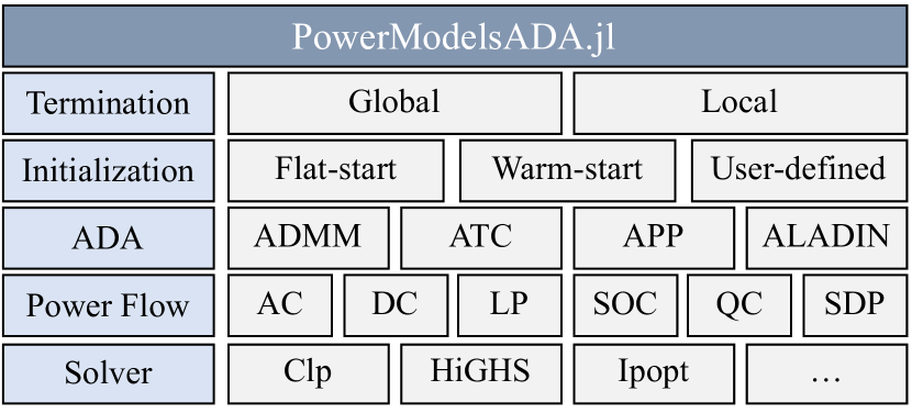
Figure 1: Illustration of PowerModelsADA options of termination methods, initializations, ADAs, power flow models, and solvers.

II Optimal Power Flow

II-A Problem Formulation

The OPF problem minimizes an objective, typically generation cost, subject to power flow and engineering constraints. While PowerModelsADA implements most of the OPF formulations supported by PowerModels, we present the AC OPF formulation for illustrative purposes:

$$\mbox{minimize}\;f_{G}:=\sum_{g\in\mathcal{G}}c_{g_{2}}\Re(S^{G}_{g})^{2}+c_{g_{1}}\Re(S^{G}_{g})+c_{g_{0}}$$ (1a)

subject to:

$$\sum_{\begin{subarray}{c}g\in\mathcal{G}_{i}\end{subarray}}\!S^{G}_{g}\!-\!\sum_{\begin{subarray}{c}l\in\mathcal{L}_{i}\end{subarray}}\!S^{L}_{l}\!-\!\sum_{\begin{subarray}{c}h\in\mathcal{H}_{i}\end{subarray}}\!\!(Y^{s}_{h})^{*}|V_{i}|^{2}\!=\!\sum_{\begin{subarray}{c}(i,j)\in\mathcal{E}\end{subarray}}\!\!\!\!S_{ij},\!\!\!\!\!\!\!\!\!\!\!\!\!\!\!\!\!\!\!\!\!\! \forall i\in\mathcal{N},$$ (1b)

$$S_{ij}=Y_{ij}^{*}V_{i}V_{i}^{*}-Y_{ij}^{*}V_{i}V_{j}^{*},\;\;\qquad\qquad\quad \forall(i,j)\in\mathcal{E},$$ (1c)

$$V_{i}^{min}\leq|V_{i}|\leq V_{i}^{max},\;\; \forall i\in\mathcal{N},$$ (1d)

$$S_{g}^{min}\leq S^{G}_{g}\leq S_{g}^{max},\;\; \forall g\in\mathcal{G},$$ (1e)

$$|S_{ij}|\leq S^{max}_{ij},\;\; \forall(i,j)\in\mathcal{E},$$ (1f)

$$\angle V_{r}=0,\;\;$$ (1g)

where $\mathcal{N}$, $\mathcal{G}$, $\mathcal{L}$, and $\mathcal{H}$ are the sets of buses, generators, loads, and shunts. The set $\mathcal{E}$ consists of branches connecting two buses with both the forward and backward directions. The subsets $\mathcal{G}_{i}\subset\mathcal{G}$, $\mathcal{L}_{i}\subset\mathcal{L}$, and $\mathcal{H}_{i}\subset\mathcal{H}$ are the corresponding elements at bus $i\in\mathcal{N}$. The decision variables are the buses’ voltage phasors $V_{i}\in\mathbb{C}$, $\forall i\in\mathcal{N}$, the generators’ power outputs $S^{G}_{g}\in\mathbb{C}$, $\forall g\in\mathcal{G}$, and the branches’ power flows $S_{ij}\in\mathbb{C}$, $\forall(i,j)\in\mathcal{E}$. The load demands are $S^{L}_{l}\in\mathbb{C}$, $\forall l\in\mathcal{L}$, branch admittances are $Y_{ij}\in\mathbb{C}$, $\forall(i,j)\in\mathcal{E}$, and shunt admittances are $Y^{s}_{h}\in\mathbb{C}$, $\forall h\in\mathcal{H}$. Each generator $g\in\mathcal{G}$ has a quadratic cost function with coefficients $c_{g_{2}}$, $c_{g_{1}}$, and $c_{g_{0}}$. We use $\Re(\,\cdot\,)$, $|\,\cdot\,|$, $\angle(\,\cdot\,)$, and $(\,\cdot\,)^{*}$ to denote the real part, magnitude, phase angle, and conjugate of complex variables. Complex-valued inequalities are interpreted element-wise on the real and imaginary parts.

Objective (1a) minimizes total generation cost. The equalities (1b)–(1c) model AC power flow. The inequalities (1d)–(1f) bound voltage magnitudes, generator outputs, and apparent power flows. Constraint (1g) sets the reference bus $r$ voltage phase angle.

The formulation in (1) is commonly called the ACOPF problem since it uses the AC power flow equations. The ACOPF (1) is non-convex and generally NP-hard [9]. Nonetheless, local non-linear solvers can often find good solutions. There are also many OPF approximations and relaxations that are more tractable than (1) [10]. PowerModelsADA builds on PowerModels’s flexibility to select the OPF formulation among the polar (ACP) and rectangular (ACR) forms, various approximations (e.g., DC power flow), and relaxations (e.g., second-order cone (SOC) and quadratic convex (QC)) [3].

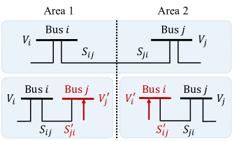
Figure 2: Two connected areas separated by the dashed line before (top) and after (bottom) decomposition.

II-B Alternating Distributed Algorithms

ADAs solve large problems by iteratively solving smaller subproblems associated with each area in the set of areas $\mathcal{A}$. An area $a\in\mathcal{A}$ is defined by a set of buses, denoted with $\mathcal{N}^{a}$, and contains the generators $\mathcal{G}^{a}$, loads $\mathcal{L}^{a}$, shunts $\mathcal{H}^{a}$, and branches $\mathcal{E}^{a}$ connected to the buses in $\mathcal{N}^{a}$. There are several decomposition strategies with differing implications for the number of variables and the convergence rate [11]. PowerModelsADA decomposes the OPF problem by introducing fictitious buses and generators at branch terminals connecting two areas as shown in Fig. 2. The fictitious generators can inject or absorb arbitrary amounts of active and reactive power with zero-cost unbounded outputs. We then impose consistency constraints between the fictitious and the original variables:

$$V_{i} =V^{\prime}_{i}, \forall i\in\mathcal{N}_{B},$$ (2a)

$$S_{ij} =S^{\prime}_{ij}, \forall(i,j)\in\mathcal{E}_{B},$$ (2b)

where the sets $\mathcal{N}_{B}$ and $\mathcal{E}_{B}$ are the boundary buses and branches. To separate the subproblems, we relax the consistency constraints (2) using an augmented Lagrangian method with a penalty on the consistency constraints’ violations multiplied by a hyperparameter and evaluate the fictitious variables with values shared by neighbors. The ADAs then 1) solve the subproblems, 2) share the boundary variable values with neighboring areas, 3) update the relaxed consistency constraints with the shared boundary variables, and 4) repeat this process until achieving consensus.

III PowerModelsADA Architecture

PowerModelsADA solves distributed OPF problems via the function solve_dopf. This function takes the system data, algorithm-specific functions and parameters, the power flow model, and the optimization solver as inputs, and returns the optimal solution of each area. The initial release of PowerModelsADA implements four ADAs: ADMM, ATC, APP, and ALADIN.

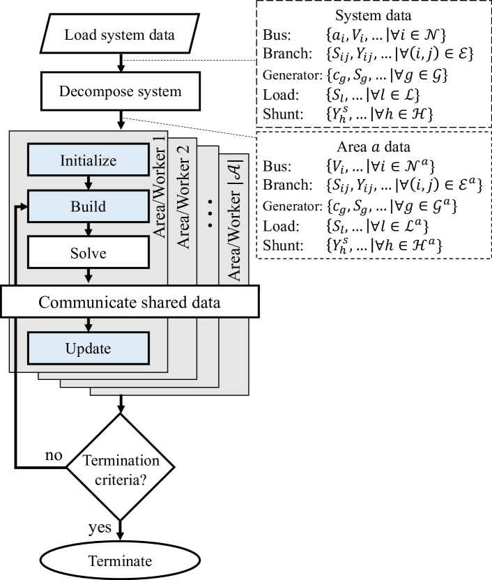
Figure 3: PowerModelsADA implementation flowchart. The boxes on the right show the data passed to the next block. The stacked Area/Worker blocks run in parallel. The light-blue blocks indicate algorithm-specific blocks.

Fig. 3 shows the PowerModelsADA algorithmic flowchart. The first two blocks denote the loading and decomposition of system data into multiple areas. The next blocks comprise the agents’ local computation, communication, and termination. The light-blue blocks in Fig. 3 are algorithm-specific blocks, while the white blocks are common to all ADAs. Implementing new ADAs with a similar algorithmic flow only requires defining the algorithm-specific blocks.

Although the algorithmic flow in Fig. 3 is used by many ADAs, PowerModelsADA also implements another algorithmic flow with a central coordinator. Further, the framework can be extended to consider other algorithmic flows (e.g., multiple hierarchical levels) by defining new solve functions. Thus, PowerModelsADA facilitates benchmarking both existing and new ADAs by defining a solve function and algorithm-specific blocks. Next, we explain the PowerModelsADA data loading, local computation, communication, and termination criteria.

III-A Data Loading and Decomposition

PowerModelsADA inherits PowerModels’ ability to load data in Matpower [12] and PTI formats, and includes a decomposition function to separate the system data into multiple areas based on the assigned area for each bus as described in Section II-B. PowerModelsADA uses dictionaries of key-value pairs for data structures, both internally and to interface with PowerModels. The inputs and outputs of the next blocks use the same data structure.

III-B Local Computation and Communication

The agents receive the area data structure, perform the local computations in parallel using the Distributed library in Julia, and synchronize by communicating their results until achieving the termination criteria. Local computations consist of four functions: initialize, build, solve, and update for the local subproblem.

Initialize is an algorithm-specific function that defines the ADA’s shared variables, iteration counter, and status (mismatches and termination criteria) as well as the shared variables’ initial values via a flat-start, a warm-start, or a user-defined method. In each iteration, the agents build their local subproblems by defining the variables, constraints, and objective. Most ADAs have the same variables and constraints, while the objective is algorithm-specific. The agents then solve their subproblem using PowerModels and store the results in the area data structure. Each agent then exchanges shared data with the neighboring areas in the communication block and stores the received data. Then, the agents update their area data structure for the next iteration.

III-C Termination

The algorithm terminates after reaching a maximum number of iterations or achieving shared variable mismatches below a specified tolerance, measured via either an $\ell_{2}$- or $\ell_{\infty}$-norm. Upon termination, the agents store the results in the area data structure. PowerModelsADA can check the termination criteria using either central or distributed methods. The central method uses a global variable to store the termination status. The distributed method requires additional iterations to allow agents to communicate the termination status with other agents and terminate the local computations simultaneously.

TABLE I: ACOPF Test Case Results

Test case	$\!\!|\mathcal{A}|$	ADMM		ATC		APP		ALADIN
		Time	Itr.	Time	Itr.	Time	Itr.	Time	Itr.
14_ieee	2	$2.1$	$28$	$2.5$	$28$	$2.4$	$31$	$2.0$	$9$
24_rts	4	$9.3$	$97$	$6.7$	$68$	$20.0$	$207$	$7.1$	$16$
30_ieee	3	$2.2$	$24$	$3.1$	$33$	$2.4$	$25$	$3.2$	$10$
30_pwl	3	$2.5$	$24$	$3.9$	$36$	$5.1$	$49$	NA	NA
39_epri	3	$9.9$	$89$	$103.0$	$761$	$101.7$	$873$	$8.4$	$20$
73_rts	3	$10.5$	$61$	$10.5$	$58$	$14.8$	$83$	$73.9$	$35$
179_goc	3	$27.0$	$66$	$16.9$	$41$	$64.6$	$166$	NC	NC
300_ieee	4	$21.4$	$65$	$30.6$	$85$	$28.5$	$77$	$1255.2$	$60$
588_sdet	8	$301.8$	$870$	$441.3$	$1136$	$462.4$	$1277$	NC	NC
2000_goc	3	$3956.2$	$671$	$9374.3$	$1353$	$5863.2$	$1006$	NC	NC
2853_sdet	38	$8293.8$	$5737$	$3973.2$	$2674$	$4901.4$	$3384$	NC	NC
4661_sdet	22	$13\,193.1$	$2951$	$14\,170.4$	$2662$	$17\,245.4$	$3747$	NC	NC

IV Test Case and Benchmarking

This section presents two use cases demonstrating the capabilities of PowerModelsADA. We first benchmarked four ADAs solving ACOPF problems (1) with 12 test systems from PGLib-OPF [13]. We then solved OPF problems using the ADMM algorithm with five power flow formulations for the 588-bus system with eight areas from PGLib-OPF [13]. See the PowerModelsADA repository [14] for the results from other ADAs with additional test cases. The results here were created with PowerModelsADA v0.3 in Julia v1.8 with the Ipopt solver on a high-performance computing platform with 16-cores and 16 GB of memory.

An ADA’s performance depends on the choice of hyperparameters that can be challenging to tune. We tuned the hyperparameters of the ADAs by starting with a large value ($10^{6}$ for ADMM and APP, and $1.2$ for ATC) and then reducing the hyperparameters gradually (dividing by $10$ for ADMM and APP, and subtracting $0.05$ for ATC) until we found a good setting. For ALADIN, we selected the hyperparameters by iterating through a range of values. We used the central termination method with an $l_{2}$-norm of the mismatch less than $0.01$ (radians and per unit), and reported the results that achieved an objective function value within $1\%$ of the solution from PowerModels.

For the ADAs benchmarked with the ACOPF formulation (1), PowerModelsADA produces the results in Table I. The columns $|\mathcal{A}|$ and “Itr.” denote the number of areas and iterations. Wall-clock computation times are given in seconds without including the data loading and code precompilation time. ALADIN failed to converge for the six cases marked with “NC”, likely due to the inherent difficulty in finding appropriate values for this algorithm’s ten hyperparameters. Also, ALADIN is inapplicable to “30_pwl” due to non-differentiability of the generators’ piecewise-linear cost functions. For the converged test cases, ALADIN has the lowest number of iterations but not necessarily the lowest computation time. Comparing across the ADAs, none of the algorithms outperform the others in all test cases.

We then solved OPF problems with five power flow formulations using the ADMM algorithm for the 588-bus system with eight areas. We repeatedly ran the test case with varying numbers of parallel computations from 1 to 10 processors. We set the value of the hyperparameter to $10^{5}$ and calculated the computation time by taking the average time of five runs. The computation time of solving the OPF problem with five power flow formulations while varying the number of processors is shown in Fig. 4. As we increase the number of processors, the computation time decreases until reaching eight processors. In some cases, the computation time increases with more processors due to the uneven assignment of the subproblems to the processors. The computation time reduces by a factor of four when using eight processors compared to a single processor. Increasing the number of processors beyond eight does not reduce the computation time because the test case has eight areas/workers such that the additional processors are not used. Comparing the power flow formulations, the DC approximation and the SOC relaxation have the fastest convergence rate.

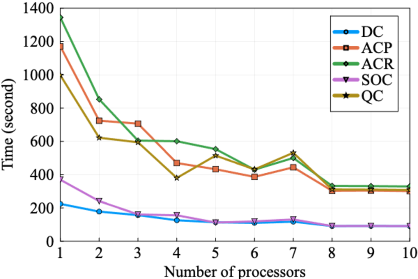
Figure 4: Computation time of solving OPF using five power flow formulations with various number of processors.

V Conclusion and Future Work

PowerModelsADA provides a plug-and-play modular framework to test and benchmark ADAs for solving OPF problems. The framework makes it straightforward to implement newly developed ADAs by defining three blocks of code (initialization, building, and updating functions). Users can then solve the OPF problem using ADAs with multiple power flow formulations and optimization solvers. Facilitating the implementation of ADAs provides many advantages to the research community for development and benchmarking.

We are pursuing several directions for extending PowerModelsADA. We intend to consider other power system optimization problems besides OPF and complete the functionality that is in PowerModels. Other possible extensions include incorporating additional decomposition and initialization methods as well as adding more ADAs.

LA-UR-23-30591

References

- [1] D. K. Molzahn et al., “A survey of distributed optimization and control algorithms for electric power systems,” IEEE Trans. Smart Grid, vol. 8, no. 6, pp. 2941–2962, 2017.
- [2] M. Alkhraijah, C. Menendez, and D. K. Molzahn, “Assessing the impacts of nonideal communications on distributed optimal power flow algorithms,” Electric Power Syst. Res., vol. 212, p. 108297, 2022, presented at 22nd Power Syst. Comput. Conf. (PSCC 2022).
- [3] C. Coffrin, R. Bent, K. Sundar, Y. Ng, and M. Lubin, “PowerModels.jl: An open-source framework for exploring power flow formulations,” in 20th Power Syst. Comput. Conf. (PSCC), 2018.
- [4] I. Dunning, J. Huchette, and M. Lubin, “JuMP: A modeling language for mathematical optimization,” SIAM Rev., vol. 59, no. 2, 2017.
- [5] S. Boyd, N. Parikh, E. Chu, B. Peleato, and J. Eckstein, “Distributed optimization and statistical learning via the alternating direction method of multipliers,” Found. Trends Mach. Learn., vol. 3, no. 1, 2010.
- [6] A. Kargarian, Y. Fu, and Z. Li, “Distributed security-constrained unit commitment for large-scale power systems,” IEEE Trans. Power Syst., vol. 30, no. 4, pp. 1925–1936, 2015.
- [7] B. Kim and R. Baldick, “Coarse-grained distributed optimal power flow,” IEEE Trans. Power Syst., vol. 12, no. 2, pp. 932–939, 1997.
- [8] A. Engelmann, Y. Jiang, T. Muhlpfordt, B. Houska, and T. Faulwasser, “Toward distributed OPF using ALADIN,” IEEE Trans. Power Syst., vol. 34, no. 1, pp. 584–594, 2019.
- [9] D. Bienstock and A. Verma, “Strong NP-hardness of AC power flows feasibility,” Oper. Res. Lett., vol. 47, no. 6, pp. 494–501, 2019.
- [10] D. K. Molzahn and I. A. Hiskens, “A survey of relaxations and approximations of the power flow equations,” Found. Trends Electric Energy Syst., vol. 4, no. 1-2, pp. 1–221, 2019.
- [11] R. Harris, M. Alkhraijah, D. Huggins, and D. K. Molzahn, “On the impacts of different consistency constraint formulations for distributed optimal power flow,” in IEEE Texas Power Energy Conf. (TPEC), 2022.
- [12] R. D. Zimmerman, C. E. Murillo-Sánchez, and R. J. Thomas, “Matpower: Steady-state operations, planning, and analysis tools for power systems research and education,” IEEE Trans. Power Syst., vol. 26, no. 1, pp. 12–19, 2011.
- [13] S. Babaeinejadsarookolaee et al., “The power grid library for benchmarking AC optimal power flow algorithms,” arXiv:1908.02788, 2019.
- [14] M. Alkhraijah, R. Harris, C. Coffrin, and D. K. Molzahn, “PowerModelsADA.jl,” https://github.com/mkhraijah/PowerModelsADA.jl, 2022.