JrCUP: Joint RIS Calibration and User Positioning for 6G Wireless Systems

Abstract

Reconfigurable intelligent surface (RIS)-assisted localization has attracted extensive attention as it can enable and enhance localization services in extreme scenarios. However, most existing works treat RISs as anchors with known positions and orientations, which is not realistic in applications with mobile or uncalibrated RISs. This work considers the joint RIS calibration and user positioning (JrCUP) problem with an active RIS. We propose a novel two-stage method to solve the considered JrCUP problem. The first stage comprises a tensor-estimation of signal parameters via rotational invariance techniques (tensor-ESPRIT), followed by a channel parameters refinement using least-squares. In the second stage, a two-dimensional search algorithm is proposed to estimate the three-dimensional user and RIS positions, one-dimensional RIS orientation, and clock bias from the estimated channel parameters. The Cramér-Rao lower bounds of the channel parameters and localization parameters are derived to verify the effectiveness of the proposed tensor-ESPRIT-based algorithms. In addition, simulation results reveal that the active RIS can significantly improve the localization performance compared to the passive case under the same system power supply in practical regions. Moreover, we observe the presence of blind areas with limited JrCUP localization performance, which can be mitigated by either leveraging more prior information or deploying extra base stations.

I Introduction

ris is an emerging technology for 5G/6G and beyond, which consists of an array of reflecting elements and offers distinctive characteristics that make the propagation environment controllable [1, 2]. With the flexibility to reshape wireless channels and the low cost of deployment, ris has become one of the key enablers for future mmwave and thz band communication systems [3, 4, 5]. Over the years, different types of ris have been proposed and widely studied, including passive ris, active ris, hybrid ris, and simultaneous transmitting and receiving (STAR) ris [6, 7, 8].

Apart from the benefits to communication, the inclusion of ris also opens new opportunities for radio localization. Radio location via wireless networks has been regarded as an indispensable function in advanced 5G/6G systems, which plays an increasingly important role in various applications. For example, radio and network localization systems in scenarios where the global positioning system (GPS) is insufficient or not available are well-studied [9, 10, 11]. A significant advantage that ris offer in radio localization is reducing the number of bs required to perform localization. A ris can not only act as a new synchronized location reference but also provide additional geometric measurements thanks to its high angular resolution. With ris being introduced properly, it is possible to perform localization using a single bs [12] or even without any bs [13, 14, 15] at all. Recent studies have shown the potential of ris-assisted localization systems in various scenarios, e.g., localization under user mobility [16], simultaneous indoor and outdoor localization [17], received-signal-strength based localization [18], etc. Besides, the position and orientation estimation error bounds for the ris-assisted localization are derived in [19]. A few ris beamforming design optimization works can be found in [20, 21, 22].

Although promising results on ris-assisted localization are shown in the literature, most of the existing works regard ris as an anchor with known position and orientation, which is not realistic in some application scenarios involving ris with calibration errors or mobile ris. As a matter of fact, calibration errors in the ris placement and geometric layout are unavoidable in practice, making ris calibration a necessity for performing a high-precision localization. The results in [23] reveal that a minor calibration error on ris geometry can cause a non-negligible model mismatch and result in performance degradation, especially in a high snr scenarios. In this context, Bayesian analysis for a ris-aided localization problem under ris position and orientation offsets is carried out in [24], which discussed the possibility of correcting the ris position and orientation under the near-field and far-field models. Recently, some efforts have also been directed towards the integration of uav and riss [25, 26], which extends the application scenarios where riss locations vary with time. In such scenarios, the localization of the ris becomes a newly introduced issue that needs to be tackled. As a consequence, localizing the ris itself while localizing the user has become an increasingly important problem to solve today.

The jrcup problem refers to localizing the ris and user simultaneously (with or without a priori information about the ris position and orientation). The 3d jrcup localization problem was first formulated in [27], which explored the relationship between the channel parameters and localization unknowns, with the corresponding Fisher information matrix derived and analyzed. Nonetheless, the adopted passive RIS in [27] limits the localization performance, and the design of an efficient channel estimator for jrcup is still missing. In [28], a multi-stage solution for the 2d jrcup problem in a hybrid ris-assisted system is reported. However, the hybrid ris setup requires an extra central processing unit (CPU) for the receiver and ris to share observations, which increases the system complexity. Recently, active ris, which can simultaneously reflect and amplify the incident signals without requiring extra CPU, has shown the potential to provide better localization performance compared to the passive ris, as it enhances the reflected signals thus avoiding the overwhelming dominance of the TX-RX los channel [29, 30, 13].

In this work, we extend the 3d jrcup problem in [27] by developing an efficient channel estimation algorithm and utilizing active ris to improve localization performance. The contributions of this work can be summarized as follows:

• We formulate the jrcup problem in an uplink simo scenario with an active ris. Motivated by the mobile ris with vertical attitude adjustment capability, we define the unknown localization parameters as the 3D position of ue, the 3D position and 1D orientation of the ris, and the clock bias between the ue and bs. By performing a localizability analysis, we show that this problem is solvable and that more dimensions of ris orientation can be estimated by introducing more ue.

• We propose a two-stage solution to the jrcup problem. In the first stage, we perform a coarse channel estimation via tensor-esprit followed by a channel parameter refinement through a ls-based algorithm. In the second stage, a 2d-search-based algorithm is proposed to estimate the localization parameters.

• The fundamental crlb for the jrcup problem are derived, which consist of the crlb for the estimations of the channel parameters and localization parameters. We show that the received noise in the active ris-involved system is colored and unknown which causes the proposed algorithm to fail to reach the theoretical bounds. However, the very minor gaps between the tested rmse and the derived crlb still show the effectiveness of our algorithms.

• Based on the derived crlb, we compare the active ris and the passive ris setups. It is shown that the active ris can outperform the passive ris within practical power supply regions. The localization performance of the active ris setup is improved with the power supply increasing up to a certain level where the performance saturates. Furthermore, we show that blind areas exist in the jrcup problem, which can be restrained by leveraging prior geometric information and/or deploying more bs.

The remainder of this paper is organized as follows. Section II introduces the system model and formulates the jrcup problem. Section III reviews the necessary mathematical preliminaries for the tensor decomposition and esprit algorithms, based on which a two-stage solution for the jrcup problem is proposed in Section IV. The crlb of the underlying estimation problems are derived in Section V. Simulation results are presented in Section VI followed by the conclusion of this work in Section VII.

Notations: Italic letters denote scalars (e.g., $a$), bold lower-case letters denote vectors (e.g., $\mathbf{a}$), bold upper-case letters denote matrices (e.g., $\mathbf{A}$), and bold calligraphic letters denote tensors (e.g., $\bm{\mathcal{A}}$). The notations $(\cdot)^{\mathsf{T}}$, $(\cdot)^{\mathsf{*}}$, $(\cdot)^{\mathsf{H}}$, $(\cdot)^{-1}$, $(\cdot)^{\dagger}$, and $\text{tr}(\cdot)$ are reserved for the transpose, conjugate, conjugate transpose, inverse, Moore-Penrose pseudo-inverse, and the matrix trace operations. The notation $\otimes$ denotes the Kronecker product, $\circ$ denotes the outer product, and $\odot$ denotes the Hadamard product. We use $[\mathbf{x}]_{i}$ to represent the $i$th entry of a vector $\mathbf{x}$, and $[\mathbf{X}]_{i,j}$ to represent the entry in the $i$th row and $j$th column of a matrix $\mathbf{X}$. The notations $\mathfrak{R}(\cdot)$ and $\mathfrak{I}(\cdot)$ denote the operations of taking the real and imaginary parts of a complex quantity, respectively.

II System Model

II-A Active ris

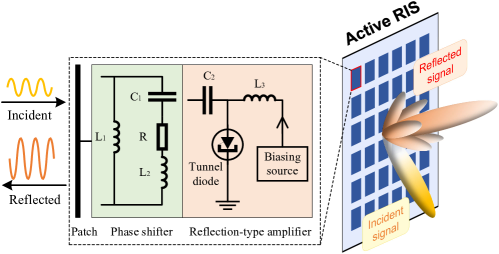
Figure 1: Schematic diagram of the hardware architecture of a typical active ris. Each ris element integrates a phase shifter [31] and a reflection-type amplifier [32].

Active ris is an array of active elements that can scatter the incident signals with both amplification and tunable phases. Fig. 1 presents a schematic diagram of the hardware architecture of a typical active ris, where the ris element consists of a phase shifter and a reflection-type amplifier [6]. Many circuit implements have been proposed to achieve the function of phase shift and amplification. For example, the phase shift can be realized through a parallel resonant circuit [31], and the amplification can be realized by a tunnel diode circuit [32], as depicted in Fig. 1. Usually, the circuit network in an active ris element can be modeled as a two-port component whose characteristics can be described by an S-parameter matrix [33]. By modulating the load impedance of each ris element, the desired amplitude and phase change can be obtained (examples can be found in, e.g., [32, 31]).

Consider an active ris of size $N_{\text{R},1}\times N_{\text{R},2}$. Assuming all the ris elements keep the same amplification coefficient, the ris profile for a transmission can be denoted as $\bm{\gamma}=p\tilde{\bm{\gamma}}$, where $p>1$ is the amplification coefficient and $\tilde{\bm{\gamma}}\in\mathbb{C}^{N_{\text{R},1}N_{\text{R},2}}$ is the phase-shift vector with unit-modulus entries. We define the incident signal power per ris element (assumed identical across ris elements) as $P_{\text{in}}$. Then the required power supply of the active ris can be calculated as [34]

$$P_{\text{R}}=(p^{2}-1)N_{\text{R},1}N_{\text{R},2}(P_{\text{in}}+\sigma_{r}^{2}),$$ (1)

where $\sigma_{r}^{2}$ denotes the power of the thermal noise introduced in each active ris element. Note that (1) is an idealized model, and the actual energy consumption of an active RIS needs to further account for the RIS mutual coupling (MC) effect, electronic circuit energy consumption, energy efficiency, etc.

II-B Geometry Model

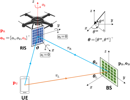
Figure 2: Illustration of an uplink simo jrcup scenario, where the states of the ue and ris are unknown. The ris is deployed on a drone with gravity sensors, where the ris is always perpendicular to the ground; hence, only one orientation angle ($[\mathbf{o}_{\text{R}}]_{3}$) needs to be estimated.

This subsection describes the geometric relationship among the system devices. Here, we only focus on the los components of the ue-bs and the ue-ris-bs paths which are used for localization, while the nlos multipath will be discussed in Subsection II-D.

We consider an uplink simo wireless system consisting of a single-antenna ue, an $N_{\text{R},1}\times N_{\text{R},2}$-element active ris, and an $N_{\text{B},1}\times N_{\text{B},2}$-element bs located at $\mathbf{p}_{\text{U}}\in\mathbb{R}^{3}$, $\mathbf{p}_{\text{R}}\in\mathbb{R}^{3}$, and $\mathbf{p}_{\text{B}}\in\mathbb{R}^{3}$, respectively, as shown in Fig. 2. The orientations of the ris and the bs are denoted as Euler angles $\mathbf{o}_{\text{R}}\in\mathbb{R}^{3}$ and $\mathbf{o}_{\text{B}}\in\mathbb{R}^{3}$. Note that the orientations can also be represented by the rotation matrices $\mathbf{R}_{\text{R}}\in\text{SO}(3)$ and $\mathbf{R}_{\text{B}}\in\text{SO}(3)$, which is constrained in the group of 3d rotations defined as $\text{SO}(3)=\{\mathbf{R}|\mathbf{R}^{\mathsf{T}}\mathbf{R}=\mathbf{I}_{3},\det(\mathbf{R})=1\}.$ The mapping between a rotation matrix and its Euler angles can be found in [5]. In this work, the states of the ue and the ris are the unknowns to be estimated, while the bs is used as the reference point in the considered coordinate system with known states. Specifically, we consider a scenario where the ris is mobile and has vertical attitude adjustment capability, making a single degree of freedom in the ris’s orientation. For example, the ris can be deployed on a drone with gravity sensors/accelerometers [37, 26]. Then we can assume the ris plane to always be perpendicular to the ground (fixed pitch and yaw angles) and only a 1D orientation (roll angle) in the horizontal plane needs to be estimated, as depicted in Fig. 2. Hence, the unknown geometric parameters consist of the 3D position of ue, the 3D position, and the 1D orientation of ris.

In the bs’s lcs, the aoa for the los path and the ris reflection path are denoted as $\bm{\theta}_{\text{L}}$ and $\bm{\theta}_{\text{R}}$. Note that each aoa pair consists of an azimuth angle and an elevation angle, i.e., $\bm{\theta}_{\text{L}}=[\theta_{\text{L}}^{\text{az}},\theta_{\text{L}}^{\text{el}}]^{\mathsf{T}}$ and $\bm{\theta}_{\text{R}}=[\theta_{\text{R}}^{\text{az}},\theta_{\text{R}}^{\text{el}}]^{\mathsf{T}}$. Those angles are related to the geometric parameters as follows:

$$\theta_{\text{L}}^{\text{az}} =\arctan 2\left([\mathbf{R}_{\text{B}}^{\mathsf{T}}(\mathbf{p}_{\text{U}}-\mathbf{p}_{\text{B}})]_{2},[\mathbf{R}_{\text{B}}^{\mathsf{T}}(\mathbf{p}_{\text{U}}-\mathbf{p}_{\text{B}})]_{1}\right),$$ (2)

$$\theta_{\text{L}}^{\text{el}} =\arcsin\left({[\mathbf{R}_{\text{B}}^{\mathsf{T}}(\mathbf{p}_{\text{U}}-\mathbf{p}_{\text{B}})]_{3}}/{\|\mathbf{p}_{\text{U}}-\mathbf{p}_{\text{B}}\|_{2}}\right).$$ (3)

A similar relationship holds for $\theta_{\text{R}}^{\text{az}}$ and $\theta_{\text{R}}^{\text{el}}$. Analogously, in the ris’s lcs, the aoa from the ue can be denoted as $\bm{\phi}_{\text{A}}=[\phi_{\text{A}}^{\text{az}},\phi_{\text{A}}^{\text{el}}]^{\mathsf{T}}$ and the aod towards the bs is $\bm{\phi}_{\text{D}}=[\phi_{\text{D}}^{\text{az}},\phi_{\text{D}}^{\text{el}}]^{\mathsf{T}}$. Furthermore, we assume an unknown clock bias $\Delta\in\mathbb{R}$ exists between the ue and bs [20, 5]. Therefore, delays over the ue-bs and the ue-ris-bs paths are given by

$$\tau_{\text{L}} ={\|\mathbf{p}_{\text{B}}-\mathbf{p}_{\text{U}}\|_{2}}/{c}+\Delta,$$ (4)

$$\tau_{\text{R}} ={\|\mathbf{p}_{\text{R}}-\mathbf{p}_{\text{U}}\|_{2}/{c}+\|\mathbf{p}_{\text{B}}-\mathbf{p}_{\text{R}}\|_{2}}/{c}+\Delta,$$ (5)

where $c$ is the speed of light.

II-C Signal Model

The bs observes and processes the uplink signals received through the ue-bs channel and the ue-ris-bs channel simultaneously. We consider the transmission of $G$ ofdm pilot symbols with $K$ subcarriers. The frequency of the $k$th subcarrier is denoted as $f_{k}=f_{c}+\frac{(2k-1-K)}{2}\Delta_{f},k=1,\dots,K$, where $f_{c}$ is the carrier frequency, $\Delta_{f}=B/K$ is the subcarrier spacing, and $B$ is the bandwidth. With reflection-type amplifiers supported by a power supply, the active ris profile at the $g$th transmission is denoted by $\bm{\gamma}_{g}=[pe^{j\beta_{1,g}},\dots,pe^{j\beta_{N_{\text{R},1}N_{\text{R},2},g}}]^{\mathsf{T}}\in\mathbb{C}^{N_{\text{R},1}N_{\text{R},2}}$, $g=1,\dots,G$, where $p>1$ denotes the amplification factor and $\beta_{n,g}$ denotes the phase shift of the $n$th ris element at the $g$th transmission. Again, here we assume that each active ris element keeps the same amplification factor. The reflection matrix of the active ris can be defined as $\bm{\Gamma}_{g}=\text{diag}(\bm{\gamma}_{g})$. Suppose that all the bs antennas are connected to an $N_{1}\times N_{2}$ rfc array. We assume $N_{1}>1$ and $N_{2}>1$. The received baseband signal for the $g$th transmission and the $k$th subcarrier, $\mathbf{y}_{g,k}\in\mathbb{C}^{N_{1}N_{2}\times 1}$, can be expressed as

$$\mathbf{y}_{g,k}=\mathbf{W}^{\mathsf{H}}\left(\mathbf{h}_{\text{L}}^{k}x_{g,k}+\mathbf{H}_{\text{R},2}^{k}\bm{\Gamma}_{g}\mathbf{h}_{\text{R},1}^{k}x_{g,k}+\mathbf{H}_{\text{R},2}^{k}\bm{\Gamma}_{g}\mathbf{n}_{r}+\mathbf{n}_{0}\right),$$ (6)

where $x_{g,k}\in\mathbb{C}$ is the transmitted signal with average transmission power $|x_{g,k}|^{2}={P_{\text{T}}}$, $\mathbf{h}_{\text{L}}^{k}$ is the ue-bs channel vector, $\mathbf{h}_{\text{R},1}^{k}$ is the ue-ris channel vector, $\mathbf{H}_{\text{R},2}^{k}$ is the ris-bs channel matrix, $\mathbf{n}_{r}\sim\mathcal{CN}(\mathbf{0},\sigma_{r}^{2}\mathbf{I})$ denotes the thermal noise introduced in the active ris, $\mathbf{n}_{0}\sim\mathcal{CN}(\mathbf{0},\sigma_{0}^{2}\mathbf{I})$ denotes the thermal noise at the receiver, and $\mathbf{W}\in\mathbb{C}^{N_{\text{B},1}N_{\text{B},2}\times N_{1}N_{2}}$ is the combiner matrix which will be specified in Subsection IV-A. Note that model (6) is reduced to the passive ris case when $p=1$ and $\sigma_{r}=0$.

According to (6), we have the total received noise for the $g$th transmission and the $k$th subcarrier as

$$\mathbf{n}_{g,k}=\mathbf{W}^{\mathsf{H}}(\mathbf{H}_{\text{R},2}^{k}\bm{\Gamma}_{g}\mathbf{n}_{r}+\mathbf{n}_{0}).$$ (7)

Here we notice the received noise $\mathbf{n}_{g,k}$ is colored and related to the unknown ris-bs channel $\mathbf{H}_{\text{R},2}^{k}$. The statistics of $\mathbf{n}_{g,k}$ will be derived in Subsection V-A. The channel model (6) can be rewritten as

$$\mathbf{y}_{g,k}=\mathbf{W}^{\mathsf{H}}\mathbf{h}_{g,k}x_{g,k}+\mathbf{n}_{g,k},$$ (8)

where $\mathbf{h}_{g,k}=\mathbf{h}_{\text{L}}^{k}+\mathbf{H}_{\text{R},2}^{k}\bm{\Gamma}_{g}\mathbf{h}_{\text{R},1}^{k}$.

II-D Channel Model

By introducing the nlos multipath, the ue-bs channel $\mathbf{h}_{\text{L}}^{k}$, the ue-ris channel $\mathbf{h}_{\text{R},1}^{k}$, and the ris-bs channel $\mathbf{H}_{\text{R},2}^{k}$ are given by [5]

$$\mathbf{h}_{\text{L}}^{k} =\sum_{i=0}^{I_{\text{L}}}\alpha_{\text{L}}^{i}e^{-j2\pi(k-1)\Delta_{f}\tau_{\text{L}}^{i}}\mathbf{a}_{\text{B}}(\bm{\theta}_{\text{L}}^{i}),$$ (9)

$$\mathbf{h}_{\text{R},1}^{k} =\sum_{i=0}^{I_{\text{R},1}}\alpha_{\text{R},1}^{i}\mathbf{a}_{\text{R}}(\bm{\phi}_{\text{A}}^{i}),$$ (10)

$$\mathbf{H}_{\text{R},2}^{k} =\sum_{i=0}^{I_{\text{R},2}}\alpha_{\text{R},2}^{i}e^{-j2\pi(k-1)\Delta_{f}\tau_{\text{R}}^{i}}\mathbf{a}_{\text{B}}(\bm{\theta}_{\text{R}}^{i})\mathbf{a}_{\text{R}}^{\mathsf{T}}(\bm{\phi}_{\text{D}}^{i}),$$ (11)

where $\mathbf{a}_{\text{B}}(\bm{\theta})\in\mathbb{C}^{N_{\text{B},1}N_{\text{B},2}}$ and $\mathbf{a}_{\text{R}}(\bm{\phi})\in\mathbb{C}^{N_{\text{R},1}N_{\text{R},2}}$ denote the array response vectors of the bs and the ris, and $\alpha_{\text{L}}^{i}$, $\alpha_{\text{R},1}^{i}$ and $\alpha_{\text{R},2}^{i}$ are the complex channel gains for the ue-bs, the ue-ris, and the ris-bs channels, respectively. Here, $i=0$ represents the los channel and the rest are the nlos multipath channels reflected by sp. The numbers of the nlos paths of the ue-bs, the ue-ris and the ris-bs channels are denoted as $I_{\text{L}}$, $I_{\text{R},1}$, and $I_{\text{R},2}$.

In this work, the multipath components are not used to perform localization, thus, it acts as a negative effect that generates additional noise. Given that, the algorithm development in this paper is based on the multipath-free model; however, the impact of the multipath effect will be evaluated in Section VI. Ignoring the multipath, the channel models (9)–(11) are reduced to

$$\mathbf{h}_{\text{L}}^{k} =\alpha_{\text{L}}e^{-j2\pi(k-1)\Delta_{f}\tau_{\text{L}}}\mathbf{a}_{\text{B}}(\bm{\theta}_{\text{L}}),$$ (12)

$$\mathbf{h}_{\text{R},1}^{k} =\alpha_{\text{R},1}\mathbf{a}_{\text{R}}(\bm{\phi}_{\text{A}}),$$ (13)

$$\mathbf{H}_{\text{R},2}^{k} =\alpha_{\text{R},2}e^{-j2\pi(k-1)\Delta_{f}\tau_{\text{R}}}\mathbf{a}_{\text{B}}(\bm{\theta}_{\text{R}})\mathbf{a}_{\text{R}}^{\mathsf{T}}(\bm{\phi}_{\text{D}}),$$ (14)

where $\alpha_{\text{L}}$, $\alpha_{\text{R},1}$ and $\alpha_{\text{R},2}$ are the complex channel gains for the corresponding los channels. The array response vectors of the bs and the ris are defined as

$$\left[\mathbf{a}_{\text{B}}(\bm{\theta})\right]_{i} =e^{j\frac{2\pi f_{c}}{c}\mathbf{t}(\bm{\theta})^{\mathsf{T}}\mathbf{p}_{\text{B},i}},$$ (15)

$$\left[\mathbf{a}_{\text{R}}(\bm{\phi})\right]_{i} =e^{j\frac{2\pi f_{c}}{c}\mathbf{t}(\bm{\phi})^{\mathsf{T}}\mathbf{p}_{\text{R},i}},$$ (16)

where $\mathbf{p}_{\text{B},i}$ and $\mathbf{p}_{\text{R},i}$ are respectively the positions of the $i$th element of the bs and the ris given in their lcs, and $\mathbf{t}(\bm{\theta})$ is the direction vector defined as $\mathbf{t}(\bm{\theta})\triangleq\begin{bmatrix}\cos(\theta^{\text{az}})\cos(\theta^{\text{el}}),\sin(\theta^{\text{az}})\cos(\theta^{\text{el}}),\sin(\theta^{\text{el}})\end{bmatrix}^{\mathsf{T}}.$ For later derivation, we assume both the antenna arrays in the bs and the ris to be upa and their element spacings are denoted as $d_{\text{B}}$ and $d_{\text{R}}$.

We assume that all the bs and ris elements are deployed on the YOZ plane of their lcs, i.e., the $x$-coordinates of these elements’ positions are zeros. Since the first entry of the $\mathbf{p}_{\text{R},i}$ is zero, we introduce the intermediate ris-related angles $\bm{\vartheta}=[\vartheta_{2},\vartheta_{3}]^{\mathsf{T}}$ as [27]

$$\vartheta_{2} =\sin(\phi_{\text{A}}^{\text{az}})\cos(\phi_{\text{A}}^{\text{el}})+\sin(\phi_{\text{D}}^{\text{az}})\cos(\phi_{\text{D}}^{\text{el}}),$$ (17)

$$\vartheta_{3} =\sin(\phi_{\text{A}}^{\text{el}})+\sin(\phi_{\text{D}}^{\text{el}}).$$ (18)

Then, the total ris array response for both signal arrival and departure can be represented through $\vartheta_{2}$ and $\vartheta_{3}$ as $\left[\mathbf{a}_{\text{R}}(\bm{\phi}_{\text{A}})\odot\mathbf{a}_{\text{R}}(\bm{\phi}_{\text{D}})\right]_{i}=e^{j\frac{2\pi f_{c}}{c}\left(\mathbf{t}(\bm{\phi}_{\text{A}})+\mathbf{t}(\bm{\phi}_{\text{D}})\right)^{\mathsf{T}}\mathbf{p}_{\text{R},i}}=e^{j\frac{2\pi f_{c}}{c}\left(\vartheta_{2}[\mathbf{p}_{\text{R},i}]_{2}+\vartheta_{3}[\mathbf{p}_{\text{R},i}]_{3}\right)}.$ Thus, a more compact formulation for the ue-ris-bs channel can be represented as

$$\mathbf{H}_{\text{R},2}^{k}\bm{\Gamma}_{g}\mathbf{h}_{\text{R},1}^{k}=\alpha_{\text{R}}\left[(\mathbf{a}_{\text{R}}(\bm{\phi}_{\text{A}})\odot\mathbf{a}_{\text{R}}(\bm{\phi}_{\text{D}}))^{\mathsf{T}}\bm{\gamma}_{g}\right]\\ \times e^{-j2\pi(k-1)\Delta_{f}\tau_{\text{R}}}\mathbf{a}_{\text{B}}(\bm{\theta}_{\text{R}}),$$ (19)

where $\alpha_{\text{R}}=\alpha_{\text{R},1}\alpha_{\text{R},2}$.

II-E Localizability Analysis and Problem Formulation

This work aims to jointly estimate the ris position and orientation, the ue position, and the clock bias based on the received signals. We adopt a two-stage estimation framework consisting of a channel parameters estimation followed by a ris and ue states estimation from the obtained channel parameters. Based on (12)–(14), we define the vector $\bm{\eta}_{\text{ch}}$ of all unknown channel parameters and the vector $\bm{\eta}$ that contains only localization-related channel parameters as

$$\bm{\eta}_{\text{ch}} \triangleq[\bm{\eta}^{\mathsf{T}},\mathfrak{R}(\alpha_{\text{L}}),\mathfrak{I}(\alpha_{\text{L}}),\mathfrak{R}(\alpha_{\text{R}}),\mathfrak{I}(\alpha_{\text{R}})]^{\mathsf{T}}\in\mathbb{R}^{12},$$ (20)

$$\bm{\eta} \triangleq[\theta_{\text{L}}^{\text{az}},\theta_{\text{L}}^{\text{el}},\theta_{\text{R}}^{\text{az}},\theta_{\text{R}}^{\text{el}},\tau_{\text{L}},\tau_{\text{R}},\vartheta_{2},\vartheta_{3}]^{\mathsf{T}}\in\mathbb{R}^{8}.$$ (21)

Note that the parameters $\alpha_{\text{L}}$ and $\alpha_{\text{R}}$ that contribute to $\bm{\eta}_{\text{ch}}$ are nuisance parameters that will not be used for solving the jrcup problem. As an objective of the general jrcup problem, the localization parameter vector that contains the ris and ue states is defined as

$$\bm{\xi}_{\text{Loc}}\triangleq[\mathbf{p}_{\text{U}}^{\mathsf{T}},\mathbf{p}_{\text{R}}^{\mathsf{T}},\mathbf{o}_{\text{R}}^{\mathsf{T}},\Delta]^{\mathsf{T}}\in\mathbb{R}^{10}.$$ (22)

The jrcup problem refers to using estimates of the channel parameters $\bm{\eta}$ to determine the state vector $\bm{\xi}_{\text{Loc}}$. However, in an estimation problem, the number of unknowns cannot exceed the number of observations $\bm{\eta}$. In the general case, it is unlikely to find a unique value of $\bm{\xi}_{\text{Loc}}$ based solely on the observations $\bm{\eta}$. The restriction of the ris orientation as highlighted in Subsection II-B reduces the unknowns pertaining to the ris orientation to a single parameter, making the number of observations equal to the number of unknowns. Consequently, the localization parameters to be estimated in this work can be redefined as

$$\bm{\xi}\triangleq[\mathbf{p}_{\text{U}}^{\mathsf{T}},\mathbf{p}_{\text{R}}^{\mathsf{T}},o_{3},\Delta]^{\mathsf{T}}\in\mathbb{R}^{8},$$ (23)

where $o_{3}=[\mathbf{o}_{\text{R}}]_{3}$ is the Euler angles of the ris orientation around the $Z$-axis; the rest of Euler angles (i.e., $o_{1}$ and $o_{2}$) are assumed to be known.

In this work, we focus on developing a solution to the jrcup problem with a single ue and 1D ris orientation. When the bs received the ofdm symbols from the ue through both los and ris reflected channels, we first estimate $\bm{\eta}$ based on the received signals $\mathbf{y}_{g,k},k=1,\dots,K,g=1,\dots,G$. Afterwards, $\bm{\xi}$ is estimated based on $\bm{\eta}$.

III Mathematical Preliminaries

To make the paper self-contained, we provide a brief review of the cp decomposition of tensors and the fundamentals of the esprit method. More details on these topics can be found in [38, 39, 40, 41].

III-A Tensors & cp Decomposition

A tensor, also known as multi-way array, is a generalization of data arrays to three or higher dimensions. Let $\bm{\mathcal{T}}\in\mathbb{C}^{I_{1}\times I_{2}\times\dots\times I_{N}}$ denote an $N$th-order tensor. The order $N$ indicates the number of dimensions, and each dimension is called a mode.

The polyadic decomposition approximates a tensor with a sum of $R$ rank-one tensors. If the number of rank-one terms $R$ is minimum, the corresponding decomposition is called a cp decomposition and the minimum achievable $R$ is referred to as the rank of the tensor. Suppose $\bm{\mathcal{T}}$ is a rank-$R$ tensor, the cp decomposition decomposes $\bm{\mathcal{T}}$ as

$$\bm{\mathcal{T}}=\sum_{r=1}^{R}\lambda_{r}\mathbf{u}_{r}^{(1)}\circ\mathbf{u}_{r}^{(2)}\circ\dots\circ\mathbf{u}_{r}^{(N)}.$$ (24)

Here, $[\mathbf{u}^{(n)}_{1},\dots,\mathbf{u}^{(n)}_{R}]=\mathbf{U}^{(n)}\in\mathbb{C}^{I_{n}\times R}$ is the factor matrix along the $n$th mode. Each matrix $\mathbf{U}^{(n)}$ has orthonormal columns. A visual representation of (24) in the third-order case ($N=3$) is shown in Fig. 3.

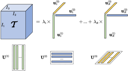
Figure 3: A cp decomposition of a rank-$R$ third-order tensor.

III-B Tensor-esprit

esprit is a search-free signal subspace-based parameter estimation technique for multidimensional harmonic retrieval, which has been widely used in channel estimation [42], spectrum sensing [43], sub-Nyquist sampling [44], etc. This subsection recaps two esprit variants, namely, element-space and beamspace tensor esprit.

Element-Space Tensor esprit: Consider a multidimensional harmonic retrieval problem with an observation tensor $\bm{\mathcal{T}}$ whose elements are given by

$$[\bm{\mathcal{T}}]_{i_{1},i_{2},\dots,i_{N}}=\sum_{r=1}^{R}\lambda_{r}\prod_{n=1}^{N}e^{j(i_{n}-1)\omega_{n,r}}.$$ (25)

To estimate the unknown angular frequencies $\omega_{n,r}$, we define

$$\mathbf{a}^{(I_{n})}(\omega_{n,r})=[1,e^{j\omega_{n,r}},\dots,e^{j(I_{n}-1)\omega_{n,r}}]^{\mathsf{T}}\in\mathbb{C}^{I_{n}},$$ (26)

$$\mathbf{A}_{n}=\big{[}\mathbf{a}^{(I_{n})}(\omega_{n,1}),\dots,\mathbf{a}^{(I_{n})}(\omega_{n,R})\big{]}\in\mathbb{C}^{I_{n}\times R}.$$ (27)

Then (25) can be rewritten as

$$\bm{\mathcal{T}}=\sum_{r=1}^{R}\lambda_{r}\mathbf{a}^{(I_{1})}(\omega_{1,r})\circ\mathbf{a}^{(I_{2})}(\omega_{2,r})\circ\dots\circ\mathbf{a}^{(I_{N})}(\omega_{N,r}).$$ (28)

We define two selection matrices $\mathbf{J}_{n,1}=\left[\mathbf{I}_{I_{n}-1},\mathbf{0}_{(I_{n}-1)\times 1}\right]\in\mathbb{R}^{(I_{n}-1)\times I_{n}},\ \mathbf{J}_{n,2}=\left[\mathbf{0}_{(I_{n}-1)\times 1},\mathbf{I}_{I_{n}-1}\right]\in\mathbb{R}^{(I_{n}-1)\times I_{n}},$ and let $\bm{\Phi}_{n}=\text{diag}\left\{[e^{j\omega_{n,1}},\dots,e^{j\omega_{n,R}}]^{\mathsf{T}}\right\}\in\mathbb{C}^{R\times R}$. To estimate the angular frequency, ESPRIT relies on the shift-invariance property of $\mathbf{A}_{n}$, which is given by

$$\mathbf{J}_{n,1}\mathbf{A}_{n}\bm{\Phi}_{n}=\mathbf{J}_{n,2}\mathbf{A}_{n}.$$ (29)

Then the associated frequencies $\omega_{n,r},r=1,\dots,R,n=1,\dots,N$, can be estimated as follows. By applying the cp decomposition to $\bm{\mathcal{T}}$, we obtain the factor matrices $\mathbf{U}^{(n)},n=1,\dots,N$. Since $\mathbf{a}^{(I_{n})}(\omega_{n,r})$ lies in the column space of $\mathbf{U}^{(n)}$, we replace $\mathbf{A}_{n}$ by $\mathbf{A}_{n}=\mathbf{U}^{(n)}\mathbf{D}_{n}$, where $\mathbf{D}_{n}\in\mathbb{C}^{R\times R}$ is a non-singular matrix. Then (29) becomes

$$\mathbf{J}_{n,1}\mathbf{U}^{(n)}\bm{\Theta}_{n}=\mathbf{J}_{n,2}\mathbf{U}^{(n)},$$ (30)

where $\bm{\Theta}_{n}=\mathbf{D}_{n}\bm{\Phi}_{n}\mathbf{D}_{n}^{-1}$. Based on (30), the ls estimate of $\bm{\Theta}_{n}$ reads [40]

$$\hat{\bm{\Theta}}_{n}=\big{(}\mathbf{J}_{n,1}\mathbf{U}^{(n)}\big{)}^{\dagger}\mathbf{J}_{n,2}\mathbf{U}^{(n)}.$$ (31)

Since the $r$th eigenvalue of ${\bm{\Theta}}_{n}$ is given by $e^{j\omega_{n,r}}$, the angular frequencies $\hat{\omega}_{n,r},r=1,\dots,R$, can be obtained from the phase components of the eigenvalues of $\hat{\bm{\Theta}}_{n}$.

Beamspace Tensor esprit: For beamspace measurements, after the $n$th-mode product of $\bm{\mathcal{T}}$ with a linear transformation matrix [45], the model (28) is modified to

$$\bm{\mathcal{T}}_{b}=\sum_{r=1}^{R}\lambda_{r}\mathbf{b}^{(J_{1})}(\omega_{1,r})\circ\mathbf{b}^{(J_{2})}(\omega_{2,r})\circ\dots\circ\mathbf{b}^{(J_{N})}(\omega_{N,r}),$$ (32)

where $\mathbf{b}^{(J_{n})}(\omega_{n,r})=\mathbf{T}_{n}^{\mathsf{H}}\mathbf{a}^{(I_{n})}(\omega_{n,r})$ with $\mathbf{T}_{n}\in\mathbb{C}^{I_{n}\times J_{n}}$. The beamspace array manifold becomes $\mathbf{B}_{n}=\big{[}\mathbf{b}^{(J_{n})}(\omega_{n,1}),\dots,\mathbf{b}^{(J_{n})}(\omega_{n,R})\big{]}\in\mathbb{C}^{J_{n}\times R}$ and $\bm{\mathcal{T}}_{b}\in\mathbb{C}^{J_{1}\times J_{2}\times\dots\times J_{n}}$.

In the beamspace model with the transformation matrix $\mathbf{T}_{n}$, generally the shift-invariance property (29) does not hold, i.e., $\mathbf{J}_{n,1}\mathbf{B}_{n}\bm{\Phi}_{n}\neq\mathbf{J}_{n,2}\mathbf{B}_{n}$. However, if $\mathbf{T}_{n}$ has a proper structure, the following proposition [46, 47] shows that the lost shift-invariance property can be restored.

Proposition 1.

Assume that $\mathbf{T}_{n}$ has a shift-invariant structure that satisfies $\mathbf{J}_{n,1}\mathbf{T}_{n}=\mathbf{J}_{n,2}\mathbf{T}_{n}\mathbf{F}_{n}$ where $\mathbf{F}_{n}\in\mathbb{C}^{J_{n}\times J_{n}}$ is a non-singular matrix and $\mathbf{T}_{n}^{\mathsf{H}}=[\mathbf{t}_{1},\dots,\mathbf{t}_{I_{n}}]^{\mathsf{T}}$. If there exists a matrix $\mathbf{Q}_{n}\in\mathbb{C}^{J_{n}\times J_{n}}$ such that

$$\begin{cases}\mathbf{Q}_{n}\mathbf{t}_{I_{n}}=\mathbf{0}_{J_{n}\times 1},\\ \mathbf{Q}_{n}\mathbf{F}_{n}^{\mathsf{H}}\mathbf{t}_{1}=\mathbf{0}_{J_{n}\times 1},\end{cases}$$ (33)

then we have

$$\mathbf{Q}_{n}\mathbf{B}_{n}\bm{\Phi}_{n}^{\mathsf{H}}=\mathbf{Q}_{n}\mathbf{F}_{n}^{\mathsf{H}}\mathbf{B}_{n},$$ (34)

where the shift-invariance property is restored.

Proof.

See Appendix A in [48]. ∎

The matrices $\mathbf{Q}_{n}$ and $\mathbf{F}_{n}$ can be estimated as [46]

$$\hat{\mathbf{Q}}_{n} =\mathbf{I}_{J_{n}}-\mathbf{t}_{I_{n}}\mathbf{t}_{I_{n}}^{\mathsf{H}}-\left(\mathbf{F}_{n}^{\mathsf{H}}\mathbf{t}_{1}\right)\left(\mathbf{F}_{n}^{\mathsf{H}}\mathbf{t}_{1}\right)^{\mathsf{H}},$$ (35)

$$\hat{\mathbf{F}}_{n} =\left(\mathbf{J}_{n,2}\mathbf{T}_{n}\right)^{\dagger}\mathbf{J}_{n,1}\mathbf{T}_{n}.$$ (36)

Then, similarly, after obtaining $\mathbf{U}^{(n)}$ by applying the cp decomposition, we can replace $\mathbf{B}_{n}$ by $\mathbf{B}_{n}=\mathbf{U}^{(n)}\mathbf{D}_{n}$, thus (34) becomes $\mathbf{Q}_{n}\mathbf{U}^{(n)}\bm{\Theta}_{n}=\mathbf{Q}_{n}\mathbf{F}_{n}^{\mathsf{H}}\mathbf{U}^{(n)}.$ Therefore,

$$\hat{\bm{\Theta}}_{n}=\big{(}\mathbf{Q}_{n}\mathbf{U}^{(n)}\big{)}^{\dagger}\mathbf{Q}_{n}\mathbf{F}_{n}^{\mathsf{H}}\mathbf{U}^{(n)}.$$ (37)

Finally, the unknown angular frequencies are obtained from the phase of the eigenvalues of $\hat{\bm{\Theta}}_{n}$.

IV Proposed Localization Method

This section develops a two-stage localization method to solve the jrcup problem formulated in Subsection II-E based on the preliminaries in Section III.

IV-A Coarse Channel Estimation via Tensor-esprit

Given $\mathbf{y}_{g,k}$ in (10), we can obtain the beamspace channel estimates by multiplying the received signals by the conjugate of the pilot symbols and dividing them by the average power as

$$\hat{\mathbf{h}}_{g,k}^{(\text{b})}=\frac{\mathbf{y}_{g,k}x_{g,k}^{*}}{P_{\text{T}}} ={\mathbf{W}^{\mathsf{H}}\mathbf{h}_{g,k}}+\Delta{\mathbf{h}}_{g,k}^{(\text{b})},$$ (38)

where $\Delta{\mathbf{h}}_{g,k}^{(\text{b})}$ is the noise term. We organize the beamspace channels as

$$\hat{\mathbf{H}} =\begin{bmatrix}\hat{\mathbf{h}}_{1,1}^{(\text{b})}&\cdots&\hat{\mathbf{h}}_{G,1}^{(\text{b})}\\ \vdots&\ddots&\vdots\\ \hat{\mathbf{h}}_{1,K}^{(\text{b})}&\cdots&\hat{\mathbf{h}}_{G,K}^{(\text{b})}\end{bmatrix}=[\hat{\mathbf{h}}_{1}^{(\text{b})},\dots,\hat{\mathbf{h}}_{G}^{(\text{b})}]\in\mathbb{C}^{KN_{1}N_{2}\times G}.$$ (39)

The goal of this subsection is to estimate the localization-related channel parameters in $\bm{\eta}$ defined in (21) given $\hat{\mathbf{H}}$.

To apply the tensor-esprit method, we design the combiner matrix $\mathbf{W}$ and the total ris profile matrix $\bm{\Gamma}$ to follow the structure

$$\mathbf{W} =\mathbf{T}_{1}\otimes\mathbf{T}_{2}\in\mathbb{C}^{N_{\text{B},1}N_{\text{B},2}\times N_{1}N_{2}},$$ (40)

$$\bm{\Upsilon} =[\bm{\gamma}_{1},\bm{\gamma}_{2},\dots,\bm{\gamma}_{G}]=\mathbf{T}_{3}\otimes\mathbf{T}_{4}\in\mathbb{C}^{N_{\text{R},1}N_{\text{R},2}\times G},$$ (41)

where $\mathbf{T}_{1}\in\mathbb{C}^{N_{\text{B},1}\times N_{1}}$, $\mathbf{T}_{2}\in\mathbb{C}^{N_{\text{B},2}\times N_{2}}$, $\mathbf{T}_{3}\in\mathbb{C}^{N_{\text{R},1}\times\sqrt{G}}$, and $\mathbf{T}_{4}\in\mathbb{C}^{N_{\text{R},2}\times\sqrt{G}}$ with $G$ thus set to a square number. Note that we utilize a fixed combiner $\mathbf{W}$ over different transmissions while the ris profile $\bm{\gamma}_{g}$ changes with $g$. Considering the structure of the array response vectors in (15), and according to (26), we can write

$$\mathbf{a}_{\text{B}}(\bm{\theta}_{\text{L}}) =\mathbf{a}^{(N_{\text{B},1})}(\omega_{\text{L},1})\otimes\mathbf{a}^{(N_{\text{B},2})}(\omega_{\text{L},2}),$$ (42)

$$\mathbf{a}_{\text{B}}(\bm{\theta}_{\text{R}}) =\mathbf{a}^{(N_{\text{B},1})}(\omega_{\text{R},1})\otimes\mathbf{a}^{(N_{\text{B},2})}(\omega_{\text{R},2}),$$ (43)

where

$$\omega_{\text{L},1} =({2\pi f_{c}d_{\text{B}}}/{c})\sin(\theta_{\text{L}}^{\text{az}})\cos(\theta_{\text{L}}^{\text{el}}),$$ (44)

$$\omega_{\text{L},2} =({2\pi f_{c}d_{\text{B}}}/{c})\sin(\theta_{\text{L}}^{\text{el}}),$$ (45)

$$\omega_{\text{R},1} =({2\pi f_{c}d_{\text{B}}}/{c})\sin(\theta_{\text{R}}^{\text{az}})\cos(\theta_{\text{R}}^{\text{el}}),$$ (46)

$$\omega_{\text{R},2} =({2\pi f_{c}d_{\text{B}}}/{c})\sin(\theta_{\text{R}}^{\text{el}}).$$ (47)

Furthermore, we define

$$\omega_{\tau_{\text{L}}}=-2\pi\Delta_{f}\tau_{\text{L}},\quad\omega_{\tau_{\text{R}}}=-2\pi\Delta_{f}\tau_{\text{R}}.$$ (48)

IV-A1 Estimating $\theta_{\text{L}}^{\text{az}},\theta_{\text{L}}^{\text{el}},\theta_{\text{R}}^{\text{az}},\theta_{\text{R}}^{\text{el}},\tau_{\text{L}},\tau_{\text{R}}$

We first use the sum of the channels over $g=1,\dots,G$, which is $\hat{\mathbf{h}}^{(\text{b})}=\sum_{g=1}^{G}\hat{\mathbf{h}}_{g}^{(\text{b})}\in\mathbb{C}^{KN_{1}N_{2}}.$ Suppose $\hat{\mathbf{h}}^{(\text{b})}=\mathbf{h}^{(\text{b})}+\Delta{\mathbf{h}}^{(\text{b})}$ with $\mathbf{h}^{(\text{b})}$ represents the true beamspace channels. The true beamspace channel $\mathbf{h}^{(\text{b})}$ can be naturally represented by a tensor $\bm{\mathcal{H}}^{{(b)}}\in\mathbb{C}^{K\times N_{1}\times N_{2}}$ as

$$\bm{\mathcal{H}}^{{(b)}}=G\alpha_{\text{L}}\mathbf{a}^{(K)}(\omega_{\tau_{\text{L}}})\circ\mathbf{T}_{1}^{\mathsf{H}}\mathbf{a}^{(N_{\text{B},1})}(\omega_{\text{L},1})\circ\mathbf{T}_{2}^{\mathsf{H}}\mathbf{a}^{(N_{\text{B},2})}(\omega_{\text{L},2})\\ +(\sum_{g=1}^{G}\beta_{\text{R},g})\mathbf{a}^{(K)}(\omega_{\tau_{\text{R}}})\circ\mathbf{T}_{1}^{\mathsf{H}}\mathbf{a}^{(N_{\text{B},1})}(\omega_{\text{R},1})\circ\mathbf{T}_{2}^{\mathsf{H}}\mathbf{a}^{(N_{\text{B},2})}(\omega_{\text{R},2}),$$ (49)

where ${{\beta}_{\text{R},g}}=\alpha_{\text{R}}\left[(\mathbf{a}_{\text{R}}(\bm{\phi}_{\text{A}})\odot\mathbf{a}_{\text{R}}(\bm{\phi}_{\text{D}}))^{\mathsf{T}}\bm{\gamma}_{g}\right].$ We can see that $\bm{\mathcal{H}}^{(\text{b})}$ is a rank-two third-order tensor based on the definition in Subsection III-A, as it is the sum of two rank-one tensors (i.e., the UE-BS channel and the UE-RIS-BS channel) and each of them is an outer product of three vectors. The first mode of $\bm{\mathcal{H}}^{(\text{b})}$ lies in the element-space while the rest of modes lie in the beamspace generated by the transformation matrices $\mathbf{T}_{1}$ and $\mathbf{T}_{2}$. Further, we can define $\bm{\Phi}_{1}=\text{diag}\left\{[e^{j\omega_{\tau_{\text{L}}}},e^{j\omega_{\tau_{\text{R}}}}]^{\mathsf{T}}\right\}$, $\bm{\Phi}_{2}=\text{diag}\left\{[e^{j\omega_{\text{L},1}},e^{j\omega_{\text{R},1}}]^{\mathsf{T}}\right\}$, and $\bm{\Phi}_{3}=\text{diag}\left\{[e^{j\omega_{\text{L},2}},e^{j\omega_{\text{R},2}}]^{\mathsf{T}}\right\}$.

To estimate the underlying angular frequencies, we first apply the cp decomposition to $\hat{\bm{\mathcal{H}}}$ (generated from $\hat{\mathbf{h}}^{(\text{b})}$) and obtain the factor matrices $\mathbf{U}^{(n)},n=1,2,3$. Then $\bm{\Theta}_{1}$ can be estimated by (31) while $\bm{\Theta}_{2}$ and $\bm{\Theta}_{3}$ can be estimated through (35), (36), and (37). Next, the estimated angular frequencies $\hat{\omega}_{\tau_{\text{L}}}$, $\hat{\omega}_{\tau_{\text{R}}}$, $\hat{\omega}_{\text{L},1}$, $\hat{\omega}_{\text{R},1}$, $\hat{\omega}_{\text{L},2}$, and $\hat{\omega}_{\text{R},2}$ can be obtained from the phases of the eigenvalues of $\hat{\bm{\Theta}}_{1}$, $\hat{\bm{\Theta}}_{2}$, and $\hat{\bm{\Theta}}_{3}$, and the corresponding channel parameters can be recovered based on (44)–(48).

IV-A2 Estimating $\vartheta_{2}$ and $\vartheta_{3}$

Based on the estimated parameters, we construct a matrix $\mathbf{R}$ as

$$\mathbf{R}=\begin{bmatrix}\mathbf{a}^{(K)}(\hat{\omega}_{\tau_{\text{L}}})\otimes\mathbf{W}^{\mathsf{H}}\mathbf{a}_{\text{B}}(\hat{\bm{\theta}}_{\text{L}})&\mathbf{a}^{(K)}(\hat{\omega}_{\tau_{\text{R}}})\otimes\mathbf{W}^{\mathsf{H}}\mathbf{a}_{\text{B}}(\hat{\bm{\theta}}_{\text{R}})\end{bmatrix}.$$

Then, we have the following system of equations:

$$\mathbf{R}[\alpha_{\text{L}},\beta_{\text{R},g}]^{\mathsf{T}}=\mathbf{h}_{g}^{(\text{b})},\ g=1,\dots,G.$$ (50)

Thus, we have a set of ls estimates $\{\hat{\alpha}_{\text{L}},\hat{\beta}_{\text{R},g}\},g=1,\dots,G$ given by

$$[\hat{\alpha}_{\text{L}},\hat{\beta}_{\text{R},g}]^{\mathsf{T}}=(\mathbf{R}^{\mathsf{H}}\mathbf{R})^{-1}\mathbf{R}^{\mathsf{H}}\mathbf{h}_{g}^{(\text{b})}.$$ (51)

Now, let

$$\hat{\mathbf{s}}_{\text{R}} =[\hat{\beta}_{\text{R},1},\hat{\beta}_{\text{R},2},\dots,\hat{\beta}_{\text{R},G}]^{\mathsf{T}}={\mathbf{s}}_{\text{R}}+\Delta{\mathbf{s}}_{\text{R}}\in\mathbb{C}^{G},$$ (52)

where ${\mathbf{s}}_{\text{R}}=[{\beta}_{\text{R},1},{\beta}_{\text{R},2},\dots,{\beta}_{\text{R},G}]^{\mathsf{T}}\in\mathbb{C}^{G}$ and $\Delta{\mathbf{s}}_{\text{R}}$ is the estimation error of $\hat{\mathbf{s}}_{\text{R}}$. By defining

$$\omega_{\vartheta_{2}}=({2\pi f_{c}d_{\text{R}}}/{c})\vartheta_{2},\quad\omega_{\vartheta_{3}}=({2\pi f_{c}d_{\text{R}}}/{c})\vartheta_{3},$$ (53)

the noise-free vector $\mathbf{s}_{\text{R}}$ can be represented as a second-order tensor (matrix) $\bm{\mathcal{S}}^{(b)}\in\mathbb{C}^{\sqrt{G}\times\sqrt{G}}$ as

$$\bm{\mathcal{S}}^{(b)} =\alpha_{\text{R}}(\mathbf{T}_{3}\otimes\mathbf{T}_{4})\Big{(}\mathbf{a}^{(N_{\text{R},1})}(\omega_{\vartheta_{2}})\otimes\mathbf{a}^{(N_{\text{R},2})}(\omega_{\vartheta_{3}})\Big{)}$$ (54)

$$=\alpha_{\text{R}}\mathbf{T}_{3}\mathbf{a}^{(N_{\text{R},1})}(\omega_{\vartheta_{2}})\circ\mathbf{T}_{4}\mathbf{a}^{(N_{\text{R},2})}(\omega_{\vartheta_{3}}).$$ (55)

Therefore, the parameters $\vartheta_{2}$ and $\vartheta_{3}$ can be estimated from $\hat{\mathbf{s}}_{\text{R}}$ using the same routine given by (35), (36), and (37).

As a summary, the complete steps of the coarse channel estimation process are presented in Algorithm 1.

Algorithm 1 Coarse Channel Estimation via Tensor-ESPRIT

0:  $\mathbf{y}_{g,k},g=1,\dots,G,k=1,\dots,K$.

0:  channel parameters estimate $\hat{\bm{\eta}}$.

1:  Obtain $\mathbf{H}=[{{\mathbf{h}}_{1}^{(\text{b})}},\dots,{{\mathbf{h}}_{G}^{(\text{b})}}]$ based on (38) and (39).

2:  Calculate $\mathbf{h}^{(\text{b})}=\sum_{g=1}^{G}{{\mathbf{h}}_{g}^{(\text{b})}}$ and form tensor $\bm{\mathcal{H}}^{(b)}$ in (49).

3:  Apply cp decomposition to $\bm{\mathcal{H}}^{(b)}$ and obtain the factor matrices $\mathbf{U}^{(n)},n=1,\dots,3$.

4:  Estimate $\hat{\bm{\Theta}}_{1}$ through (31) and obtain $\{\hat{\omega}_{\tau_{\text{L}}},\hat{\omega}_{\tau_{\text{R}}}\}$ from the phases of the eigenvalues of $\hat{\bm{\Theta}}_{1}$.

5:  Estimate $\hat{\bm{\Theta}}_{2}$ and $\hat{\bm{\Theta}}_{3}$ through (35)–(37), and obtain $\{\hat{\omega}_{\text{L},1},\hat{\omega}_{\text{R},1},\hat{\omega}_{\text{L},2},\hat{\omega}_{\text{R},2}\}$ from the phases of the eigenvalues of $\hat{\bm{\Theta}}_{2}$ and $\hat{\bm{\Theta}}_{3}$.

6:  Recover $\{\hat{\theta}_{\text{L}}^{\text{az}},\hat{\theta}_{\text{L}}^{\text{el}},\hat{\theta}_{\text{R}}^{\text{az}},\hat{\theta}_{\text{R}}^{\text{el}},\hat{\tau}_{\text{L}},\hat{\tau}_{\text{R}}\}$ based on (44)–(48).

7:  Obtain $\mathbf{s}_{\text{R}}$ by (51) and form tensor $\bm{\mathcal{S}}^{(b)}$ in (54).

8:  Obtain $\{\hat{\omega}_{\vartheta_{2}},\hat{\omega}_{\vartheta_{3}}\}$ by applying cp decomposition and repeating Step 5 to $\bm{\mathcal{S}}^{(b)}$.

9:  Recover $\{\hat{\vartheta}_{2},\hat{\vartheta}_{3}\}$ based on (53).

10:  Return $\hat{\bm{\eta}}=[\hat{\theta}_{\text{L}}^{\text{az}},\hat{\theta}_{\text{L}}^{\text{el}},\hat{\theta}_{\text{R}}^{\text{az}},\hat{\theta}_{\text{R}}^{\text{el}},\hat{\tau}_{\text{L}},\hat{\tau}_{\text{R}},\hat{\vartheta}_{2},\hat{\vartheta}_{3}]^{\mathsf{T}}$.

IV-B Channel Parameters Refinement via Least Squares

Channel parameter estimates $\tilde{\bm{\eta}}$ are refined based on the ls criterion initialized using the coarse estimates from Subsection IV-A. By defining

$$\bm{\mu}_{\text{L}}^{g,k} =\mathbf{W}^{\mathsf{H}}e^{-j2\pi(k-1)\Delta_{f}\tau_{\text{L}}}\mathbf{a}_{\text{B}}(\bm{\theta}_{\text{L}})x_{g,k},$$ (56)

$$\bm{\mu}_{\text{R}}^{g,k} =\mathbf{W}^{\mathsf{H}}\left[(\mathbf{a}_{\text{R}}(\bm{\phi}_{\text{A}})\odot\mathbf{a}_{\text{R}}(\bm{\phi}_{\text{D}}))^{\mathsf{T}}\bm{\gamma}_{g}\right]$$ (57)

$$\qquad\qquad\times e^{-j2\pi(k-1)\Delta_{f}\tau_{\text{R}}}\mathbf{a}_{\text{B}}(\bm{\theta}_{\text{R}})x_{g,k},$$ (58)

we have the noise-free signals given by

$${\bm{\mu}}_{g,k}=\alpha_{\text{L}}\bm{\mu}_{\text{L}}^{g,k}+\alpha_{\text{R}}\bm{\mu}_{\text{R}}^{g,k}.$$ (59)

We further define vectors $\{\mathbf{y},\bm{\mu}_{\text{L}},\bm{\mu}_{\text{R}}\}\in\mathbb{C}^{GKN_{1}N_{2}}$ as the concatenation of $\mathbf{y}_{g,k}$, $\bm{\mu}_{\text{L}}^{g,k}$ and $\bm{\mu}_{\text{R}}^{g,k}$ over $g=1,\dots,G,k=1,\dots,K.$ Since the noise in (8) is colored with unknown statistics, we perform a sub-optimal estimator based on the ls criterion as

$$\hat{\bm{\eta}}_{\text{LS}}=\arg\min_{\bm{\eta}}\ \|\mathbf{y}-\alpha_{\text{L}}\bm{\mu}_{\text{L}}(\bm{\eta})-\alpha_{\text{R}}\bm{\mu}_{\text{R}}(\bm{\eta})\|_{2}^{2}.$$ (60)

The value of the complex channel gains $\alpha_{\text{L}}$ and $\alpha_{\text{R}}$ can be obtained as a function of $\mathbf{y}$, $\bm{\mu}_{\text{L}}$ and $\bm{\mu}_{\text{R}}$ by solving

$$\left\{\begin{array}[]{l}{\partial\|\mathbf{y}-\alpha_{\text{L}}\bm{\mu}_{\text{L}}(\bm{\eta})-\alpha_{\text{R}}\bm{\mu}_{\text{R}}(\bm{\eta})\|_{2}^{2}}/{\partial\mathfrak{R}(\alpha_{\text{L}})}=0,\\ {\partial\|\mathbf{y}-\alpha_{\text{L}}\bm{\mu}_{\text{L}}(\bm{\eta})-\alpha_{\text{R}}\bm{\mu}_{\text{R}}(\bm{\eta})\|_{2}^{2}}/{\partial\mathfrak{R}(\alpha_{\text{R}})}=0,\end{array}\right.$$ (61)

which give

$$\hat{\alpha}_{\text{L}} =\frac{\bm{\mu}_{\text{L}}^{\mathsf{H}}\mathbf{y}\|\bm{\mu}_{\text{R}}\|_{2}^{2}-\bm{\mu}_{\text{R}}^{\mathsf{H}}\mathbf{y}\bm{\mu}_{\text{L}}^{\mathsf{H}}\bm{\mu}_{\text{R}}}{\|\bm{\mu}_{\text{L}}\|_{2}^{2}\|\bm{\mu}_{\text{R}}\|_{2}^{2}-|\bm{\mu}_{\text{L}}^{\mathsf{H}}\bm{\mu}_{\text{R}}|^{2}},$$ (62)

$$\hat{\alpha}_{\text{R}} =\frac{\bm{\mu}_{\text{R}}^{\mathsf{H}}\mathbf{y}\|\bm{\mu}_{\text{L}}\|_{2}^{2}-\bm{\mu}_{\text{L}}^{\mathsf{H}}\mathbf{y}\bm{\mu}_{\text{R}}^{\mathsf{H}}\bm{\mu}_{\text{L}}}{\|\bm{\mu}_{\text{L}}\|_{2}^{2}\|\bm{\mu}_{\text{R}}\|_{2}^{2}-|\bm{\mu}_{\text{L}}^{\mathsf{H}}\bm{\mu}_{\text{R}}|^{2}}.$$ (63)

Then, (60) can be solved by using, e.g., gradient descent method given the initialization $\hat{\bm{\eta}}$. We denote the refined localization-related channel parameters as $\tilde{\bm{\eta}}$.

IV-C Conversion to the Localization Domain

Based on the refined channel parameters estimates $\tilde{\bm{\eta}}$, the localization parameters $\bm{\xi}$ can be recovered by carrying out a 2D search over $o_{3}$ and $\Delta$; the rest of the localization parameters can be determined from each search point $[o_{3},\Delta]^{\mathsf{T}}$ and a cost metric can be defined to compare the fitness of different search points, as will be explained imminently.

Given channel parameters $[\theta_{\text{L}}^{\text{az}},\theta_{\text{L}}^{\text{el}},\theta_{\text{R}}^{\text{az}},\theta_{\text{R}}^{\text{el}},\tau_{\text{L}},\tau_{\text{R}},\vartheta_{2},\vartheta_{3}]^{\mathsf{T}}$ and any $\check{o}_{3}$ and $\check{\Delta}$, we can first determine the propagation distance of the los ue-bs path and ris reflection path as

$$\check{d}_{\text{L}}=c(\tau_{\text{L}}-\check{\Delta}),\qquad\check{d}_{\text{R}}=c(\tau_{\text{R}}-\check{\Delta}).$$ (64)

which further determine the ue position as

$$\check{\mathbf{p}}_{\text{U}}=\mathbf{p}_{\text{B}}+\check{d}_{\text{L}}\mathbf{R}_{\text{B}}\mathbf{t}(\theta_{\text{L}}^{\text{az}},\theta_{\text{L}}^{\text{el}}).$$ (65)

The ris position can be obtained as the intersection of the ellipsoid $\|\check{\mathbf{p}}_{\text{R}}-\mathbf{p}_{\text{B}}\|_{2}+\|\check{\mathbf{p}}_{\text{R}}-\check{\mathbf{p}}_{\text{U}}\|_{2}=\check{d}_{\text{R}}$ and the line $\check{\mathbf{p}}_{\text{R}}=\mathbf{p}_{\text{B}}+x\mathbf{R}_{\text{B}}\mathbf{t}(\theta_{\text{R}}^{\text{az}},\theta_{\text{R}}^{\text{el}})$, with $x>0$ being the distance between bs and ris. The intersection is determined by solving for $x$ to obtain

$$x=\frac{\check{d}_{\text{R}}^{2}-\|\mathbf{p}_{\text{B}}-\check{\mathbf{p}}_{\text{U}}\|_{2}^{2}}{2\left(\check{d}_{\text{R}}+(\mathbf{R}_{\text{B}}\mathbf{t}(\theta_{\text{R}}^{\text{az}},\theta_{\text{R}}^{\text{el}}))^{\mathsf{T}}(\mathbf{p}_{\text{B}}-\check{\mathbf{p}}_{\text{U}})\right)}.$$ (66)

Then, we can predict the intermediate measurements $\{\check{\vartheta}_{2},\check{\vartheta}_{3}\}$ according to (17) and (18) based on $\check{o}_{3}$, $\check{\mathbf{p}}_{\text{U}}$, $\check{\mathbf{p}}_{\text{R}}$ and ${\mathbf{p}}_{\text{B}}$. Thus, we can compute the cost metric as

$$f(\check{o}_{3},\check{\Delta})=\big{\|}[\check{\vartheta}_{2},\check{\vartheta}_{3}]^{\mathsf{T}}-[\hat{\vartheta}_{2},\hat{\vartheta}_{3}]^{\mathsf{T}}\big{\|}_{2}^{2},$$ (67)

which allows us to perform a 2d search over all the $\{o_{3},\Delta\}$ candidates in a pre-defined search space. The optimal values that minimize $f(\check{o}_{3},\check{\Delta})$ in (67) are then returned as the estimated $\hat{o_{3}}$ and $\hat{\Delta}$, and the corresponding $\hat{\mathbf{p}}_{\text{U}}$ and $\hat{\mathbf{p}}_{\text{R}}$ can be determined accordingly.

Let $\{\mathcal{P}_{o_{3}},\mathcal{P}_{\Delta}\}$ denotes the search spaces and $\{d_{o_{3}},d_{\Delta}\}$ denotes the search resolutions. We can further perform multiple rounds of search grid refinement. As an example, for the $i$th round refined search over the search space $\{\mathcal{P}_{o_{3}}^{i},\mathcal{P}_{\Delta}^{i}\}$ and resolution $\{d_{o_{3}}^{i},d_{\Delta}^{i}\}$ that returns estimates $\{\hat{o}_{3}^{i},\hat{\Delta}^{i}\}$, we can shrink the resolution and the search space in round $i+1$ such that

$$d_{o_{3}}^{i+1} =\kappa d_{o_{3}}^{i},\qquad d_{\Delta}^{i+1}=\kappa d_{\Delta}^{i},$$ (68)

$$\mathcal{P}_{o_{3}}^{i+1} =\{\dots,\hat{o}_{3}^{i}-d_{o_{3}}^{i+1},\hat{o}_{3}^{i},\hat{o}_{3}^{i}+d_{o_{3}}^{i+1},\dots\},$$ (69)

$$\mathcal{P}_{\Delta}^{i+1} =\{\dots,\hat{\Delta}^{i}-d_{\Delta}^{i+1},\hat{\Delta}^{i},\hat{\Delta}^{i}+d_{\Delta}^{i+1},\dots\},$$ (70)

where $\kappa\in(0,1)$ and the cardinalities of $\mathcal{P}_{o_{3}}^{i}$ and $\mathcal{P}_{\Delta}^{i}$ are fixed as $\mathrm{card}(\mathcal{P}_{o_{3}}^{i})=C_{o_{3}}$ and $\mathrm{card}(\mathcal{P}_{\Delta}^{i})=C_{\Delta}$ for all $i$ values. The pseudo-code of the proposed search method is summarized in Algorithm 2.

Algorithm 2 2D Search-Based Localization Algorithm

0:  refined channel parameters $\tilde{\bm{\eta}}$, number of refinement $Q$.

0:  localization parameters estimates $\hat{\bm{\xi}}$.

1:  Initialize search space and resolution $\{\mathcal{P}_{o_{3}}^{0},\mathcal{P}_{\Delta}^{0},d_{o_{3}}^{0},d_{\Delta}^{0}\}$.

2:  for $i=0,\dots,Q$ do

3:     for every candidate $\check{o}_{3}\in\mathcal{P}_{o_{3}}^{i}$ do

4:        for every candidate $\check{\Delta}\in\mathcal{P}_{\Delta}^{i}$ do

5:           Compute $\check{d}_{\text{L}}$ and $\check{d}_{\text{R}}$ through (64).

6:           Estimate ue position $\check{\mathbf{p}}_{\text{U}}$ through (65) and estimate ris position $\check{\mathbf{p}}_{\text{R}}$ through (66).

7:           Predict the intermediate measurements $\{\check{\vartheta}_{2},\check{\vartheta}_{3}\}$ based on $\check{o}_{3}$, $\check{\mathbf{p}}_{\text{U}}$, $\check{\mathbf{p}}_{\text{R}}$ and ${\mathbf{p}}_{\text{B}}$.

8:           Compute the cost metric $f(\check{o}_{3},\check{\Delta})$ based on (67).

9:        end for

10:     end for

11:     Select the candidate pair $\{\hat{o}_{3}^{i},\hat{\Delta}^{i}\}$ that minimize $f({o}_{3},{\Delta})$ and determine $\hat{\mathbf{p}}_{\text{U}}^{i}$ and $\hat{\mathbf{p}}_{\text{R}}^{i}$ based on $\{\hat{o}_{3}^{i},\hat{\Delta}^{i}\}$.

12:     Shrink $\{\mathcal{P}_{o_{3}}^{i+1},\mathcal{P}_{\Delta}^{i+1},d_{o_{3}}^{i+1},d_{\Delta}^{i+1}\}$ by (68)–(70).

13:  end for

14:  Return $\hat{\bm{\xi}}=[(\hat{\mathbf{p}}_{\text{U}}^{Q})^{\mathsf{T}},(\hat{\mathbf{p}}_{\text{R}}^{Q})^{\mathsf{T}},\hat{o}_{3}^{Q},\hat{\Delta}^{Q}]^{\mathsf{T}}$.

IV-D Complexity Analysis

This subsection evaluates the computational complexity of the proposed algorithms. Among the proposed method, Algorithm 1 involves the channel matrix recovery with a complexity $\mathcal{O}(KGN_{1}N_{2})$, the cp decomposition of $\bm{\mathcal{H}}^{(b)}$ and the corresponding matrix multiplications with a complexity $\mathcal{O}(KN_{1}N_{2})+\mathcal{O}(K^{2})+\mathcal{O}(N_{1}^{2})+\mathcal{O}(N_{2}^{2})$, and the cp decomposition of $\bm{\mathcal{S}}^{(b)}$ and the corresponding matrix multiplications with a complexity $\mathcal{O}(G)$. The ls refinement of the channel parameters performs an iterative procedure, which gives a complexity $\mathcal{O}(TKGN_{1}N_{2})$ where $T$ denotes the total number of iterations. Finally, a complexity of $\mathcal{O}(QC_{o_{3}}C_{\Delta})$ is introduced by Algorithm 2. In summary, the overall complexity of the proposed solution for the jrcup problem is given by

$$\mathcal{O}_{\text{total}}=\mathcal{O}(K^{2})+\mathcal{O}(N_{1}^{2})+\mathcal{O}(N_{2}^{2})\\ +\mathcal{O}(TKGN_{1}N_{2})+\mathcal{O}(QC_{o_{3}}C_{\Delta}).$$ (71)

V Localization Error Bounds Derivation

V-A crlb for Channel Parameters Estimation

Considering the fact that the received noise (7) is zero-mean noncircular complex Gaussian random variables, the fim of all the unknown channel parameters $\bm{\eta}_{\text{ch}}$ is given by the following Proposition 2.

Proposition 2.

Based on the channel model (7), (8) and (59), the fim of channel parameters $\bm{\eta}_{\text{ch}}$ can be computed as

$$\mathbf{J}({\bm{\eta}}_{\text{ch}}) =\sum^{G}_{g=1}\sum^{K}_{k=1}\mathbf{D}_{g,k}^{\mathsf{T}}\left[\mathbf{C}_{0}+\mathbf{C}_{r}^{g,k}\right]^{-1}\mathbf{D}_{g,k},$$ (72)

where

$$\mathbf{D}_{g,k} =\bigg{[}\mathfrak{R}\left(\frac{\partial{\bm{\mu}}_{g,k}}{\partial{\bm{\eta}}_{\text{ch}}}\right)^{\mathsf{T}},\ \mathfrak{I}\left(\frac{\partial{\bm{\mu}}_{g,k}}{\partial{\bm{\eta}}_{\text{ch}}}\right)^{\mathsf{T}}\bigg{]}^{\mathsf{T}},$$ (73)

$$\mathbf{C}_{0} =\frac{\sigma_{0}^{2}}{2}\begin{bmatrix}\mathfrak{R}\left(\mathbf{A}_{0}\mathbf{A}_{0}^{\mathsf{H}}\right)&\mathfrak{I}\left(\mathbf{A}_{0}\mathbf{A}_{0}^{\mathsf{H}}\right)^{\mathsf{T}}\vspace{0.3em}\\ \mathfrak{I}\left(\mathbf{A}_{0}\mathbf{A}_{0}^{\mathsf{H}}\right)&\mathfrak{R}\left(\mathbf{A}_{0}\mathbf{A}_{0}^{\mathsf{H}}\right)\end{bmatrix},$$ (74)

$$\mathbf{C}_{r}^{g,k} =\frac{\sigma_{r}^{2}}{2}\begin{bmatrix}\mathfrak{R}\left(\mathbf{A}_{r}^{g,k}(\mathbf{A}_{r}^{g,k})^{\mathsf{H}}\right)&\mathfrak{I}\left(\mathbf{A}_{r}^{g,k}(\mathbf{A}_{r}^{g,k})^{\mathsf{H}}\right)^{\mathsf{T}}\vspace{0.3em}\vspace{0.2em}\\ \mathfrak{I}\left(\mathbf{A}_{r}^{g,k}(\mathbf{A}_{r}^{g,k})^{\mathsf{H}}\right)&\mathfrak{R}\left(\mathbf{A}_{r}^{g,k}(\mathbf{A}_{r}^{g,k})^{\mathsf{H}}\right)\end{bmatrix},$$ (75)

with $\mathbf{A}_{0}=\mathbf{W}^{\mathsf{H}}$ and $\mathbf{A}_{r}^{g,k}=\mathbf{W}^{\mathsf{H}}\mathbf{H}_{\text{R},2}^{k}\bm{\Gamma}_{g}$.

Proof.

See Appendix A ∎

Remark 1.

Note that in (72), the covariance matrix $\mathbf{C}_{r}^{g,k}$ is a function of ${\bm{\eta}}_{\text{ch}}$, which also contributes to the fim of ${\bm{\eta}}_{\text{ch}}$ in principle [49, B.3.3]. Nonetheless, since the noise statistics information is not used in the channel estimation processes in Subsection IV-A and IV-B, we ignore this relationship in this work.

Based on (72), we can compute the fim of localization-related parameters $\bm{\eta}$ using Schur’s complement: we partition $\mathbf{J}(\bm{\eta}_{\text{ch}})=[\mathbf{X},\mathbf{Y};\mathbf{Y}^{\mathsf{T}},\mathbf{Z}]$, where $\mathbf{X}\in\mathbb{R}^{8\times 8}$ so that $\mathbf{J}(\bm{\eta})=\mathbf{X}-\mathbf{Y}\mathbf{Z}^{-1}\mathbf{Y}^{\mathsf{T}}$. Then the estimation error bounds for $\bm{\theta}_{\text{L}}$, $\bm{\theta}_{\text{R}}$, $\tau_{\text{L}}$, $\tau_{\text{R}}$ and $\bm{\vartheta}$ can be derived as

$$\mathrm{EB}(\bm{\theta}_{\text{L}}) =\sqrt{\text{tr}([\mathbf{J}({\bm{\eta}})^{-1}]_{1:2,1:2})},$$ (76)

$$\mathrm{EB}(\bm{\theta}_{\text{R}}) =\sqrt{\text{tr}([\mathbf{J}({\bm{\eta}})^{-1}]_{3:4,3:4})},$$ (77)

$$\mathrm{EB}(\tau_{\text{L}}) =\sqrt{[\mathbf{J}({\bm{\eta}})^{-1}]_{5,5}},$$ (78)

$$\mathrm{EB}(\tau_{\text{R}}) =\sqrt{[\mathbf{J}({\bm{\eta}})^{-1}]_{6,6}},$$ (79)

$$\mathrm{EB}(\bm{\vartheta}) =\sqrt{\text{tr}([\mathbf{J}({\bm{\eta}})^{-1}]_{7:8,7:8})},$$ (80)

which lower bound the estimation rmse for the corresponding parameters.

V-B crlb for Localization Parameters Estimation

Based on the calculated $\mathbf{J}({\bm{\eta}})$ and the geometric model in (2)–(5) and (17)–(18), we can further derive the fim of the localization parameters $\bm{\xi}$ using the chain rule of the fim transformation as [50]

$$\mathbf{J}({\bm{\xi}})=\mathbf{T}^{\mathsf{T}}\mathbf{J}({\bm{\eta}})\mathbf{T},$$ (81)

where $\mathbf{T}=\partial\bm{\eta}/\partial\bm{\xi}\in\mathbb{R}^{8\times 8}$ is the Jacobian matrix. Then the lower bounds for the estimation rmse of $\mathbf{p}_{\text{U}}$, $\mathbf{p}_{\text{R}}$, $o_{3}$ are

$$\mathrm{EB}(\mathbf{p}_{\text{U}}) =\sqrt{\text{tr}([\mathbf{J}({\bm{\xi}})^{-1}]_{1:3,1:3})},$$ (82)

$$\mathrm{EB}(\mathbf{p}_{\text{R}}) =\sqrt{\text{tr}([\mathbf{J}({\bm{\xi}})^{-1}]_{4:6,4:6})},$$ (83)

$$\mathrm{EB}(o_{3}) =\sqrt{[\mathbf{J}({\bm{\xi}})^{-1}]_{7,7}}.$$ (84)

VI Numerical Results

VI-A Evaluation Setup

TABLE I: Default Simulation Parameters

Parameter	Value
Propagation Speed $c$	$2.9979\times 10^{8}\,\mathrm{m/s}$
Carrier Frequency $f_{c}$	$28\,\mathrm{GHz}$
Bandwidth $B$	$100\,\mathrm{MHz}$
# Subcarriers $K$	$32$
# Transmissions $G$	$9$
Clock Offset $\rho$	$100\,\mathrm{ns}$
Transmission Power $P_{\text{T}}$	$10\,\mathrm{dBm}$
Active RIS Power $P_{\text{R}}$	$7\,\mathrm{dBm}$
Noise PSD of Receiver & RIS	$-174\,\mathrm{dBm/Hz}$
Noise Figure of Receiver & ris	$10\,\mathrm{dB}$
Array Size of bs / rfc / ris	$10\times 10$ / $5\times 5$ / $15\times 15$
Position & Orientation of bs	$\mathbf{p}_{\text{B}}=[0,5,3]^{\mathsf{T}}$, $\mathbf{o}_{\text{B}}=[0,0,-\pi/2]^{\mathsf{T}}$
Position & Orientation of ris	$\mathbf{p}_{\text{R}}=[-5,0,3]^{\mathsf{T}}$, $\mathbf{o}_{\text{R}}=[0,0,0]^{\mathsf{T}}$
Position of ue	$\mathbf{p}_{\text{B}}=[3,2,1]^{\mathsf{T}}$

We consider an indoor localization scenario within a $10\,\mathrm{m}\times 10\,\mathrm{m}\times 3\,\mathrm{m}$ space. We use random signal symbols $x_{g,k}$ with the power constraint $|x_{g,k}|=\sqrt{P_{\text{T}}}$, and random precoder $\mathbf{W}$ and ris profiles $\bm{\Upsilon}$ satisfying the structure constraints (40) and (41). Based on (1), the active ris amplification factor $p$ is calculated as

$$p=\sqrt{\frac{P_{\text{R}}}{N_{\text{R},1}N_{\text{R},2}(P_{\text{T}}|\alpha_{\text{R},1}|^{2}+\sigma_{r}^{2})}+1}.$$ (85)

The channel gains of the los ue-bs, ue-ris and ris-bs paths are generated by $\alpha_{\text{L}}=\frac{\lambda_{c}}{4\pi\|\mathbf{p}_{\text{U}}-\mathbf{p}_{\text{B}}\|_{2}}e^{j\psi_{\text{L}}},\ \alpha_{\text{R},1}=\frac{\lambda_{c}}{4\pi\|\mathbf{p}_{\text{U}}-\mathbf{R}_{\text{R}}\|_{2}}e^{j\psi_{\text{R},1}},\ \alpha_{\text{R},2}=\frac{\lambda_{c}}{4\pi\|\mathbf{p}_{\text{R}}-\mathbf{R}_{\text{B}}\|_{2}}e^{j\psi_{\text{R},2}},$ where $\lambda_{c}=c/f_{c}$ and $\psi_{\text{L}}$, $\psi_{\text{R},1}$ and $\psi_{\text{R},2}$ are independently generated from a uniform distribution $\mathcal{U}(0,2\pi)$. When the multipath effect is introduced, as an example, the channel gains of the nlos paths between the ue and bs in (9) are set as $\alpha_{\text{L}}^{i}=\frac{\sqrt{4\pi c_{\text{L},i}}\lambda_{c}}{16\pi^{2}d_{\text{U},i}d_{\text{B},i}}e^{j\psi_{\text{L},i}},\ i=1,\dots,I_{\text{L}}$, where $c_{\text{L},i}$ represents the radar cross section (RCS) coefficient and $\psi_{\text{L},i}$ is the random phase. Here, $d_{\text{U},i}$ and $d_{\text{B},i}$ are the distances between the ue and the $i$th sp and the distance between the bs and the $i$th sp. The channel gains $\alpha_{\text{R},1}^{i}$ and $\alpha_{\text{R},2}^{i}$ in (10) and (11) are defined in a similar manner. In addition, we define the received snr as

$$\mathrm{SNR}\triangleq\frac{\sum_{g=1}^{G}\sum_{k=1}^{K}\|{\bm{\mu}}_{g,k}\|_{2}^{2}}{\sum_{g=1}^{G}\sum_{k=1}^{K}\text{tr}(\mathbf{C}_{0}+\mathbf{C}_{r}^{g,k})}.$$ (86)

In this paper, the three Euler angles, i.e. $[\mathbf{o}]_{1}$, $[\mathbf{o}]_{2}$ and $[\mathbf{o}]_{3}$, represent the rotations around $X$-axis, $Y$-axis and $Z$-axis, respectively. The default orientation $\mathbf{o}=[0,0,0]^{\mathsf{T}}$ is set to face the positive $X$-axis. The element spacings of the bs and ris are set as $0.5\,\mathrm{\lambda_{c}}$ and $0.2\,\mathrm{\lambda_{c}}$, respectively. Other default simulation parameters are listed in Table I. Throughout the simulation examples, all the involved rmse are computed over 500 Monte Carlo trials. The channel delays and the clock bias are presented in units of meters by multiplying them by the constant propagation speed $c$ for better intuition.

VI-B Performance Evaluation of the Proposed Algorithms

Figure 4: The evaluation of rmse of $\bm{\theta}_{\text{L}}$, $\bm{\theta}_{\text{R}}$, $\tau_{\text{L}}$, $\tau_{\text{R}}$ and $\bm{\vartheta}$ versus received snr for the existing SOMP algorithm, the proposed tensor-ESPRIT coarse estimation, and the proposed ls-based refinement.

Figure 5: The evaluation of rmse of $\mathbf{p}_{\text{U}}$, $\mathbf{p}_{\text{R}}$ and $o_{3}$ versus received snr for different numbers ($0,1,2,3$) of grid refinements.

VI-B1 Channel Estimation Performance

We first evaluate the performance of the proposed channel estimators. To provide a benchmark in addition to the crlb, the proposed channel estimator is compared with the existing simultaneous orthogonal matching pursuit (SOMP) algorithm which has been verified to offer better channel estimation performance than the original orthogonal matching pursuit (OMP) algorithm [51]. We use SOMP to estimate the two strongest paths as the ue-bs and the ue-ris-bs channels. For implementation details of SOMP, the readers are referred to [51, 52]. To meet the restricted isometry property [53] that SOMP requires, we use random combiner $\mathbf{W}$ and random ris profile $\bm{\Upsilon}$ when performing SOMP, while the proposed $\{\mathbf{W},\bm{\Upsilon}\}$ in (40) and (41) are used when evaluating the proposed methods. We derive and present the crlb for both cases. The SOMP dictionary sizes for each parameter in $\{\bm{\theta}_{\text{L}},\bm{\theta}_{\text{R}},\tau_{\text{L}},\tau_{\text{R}},\bm{\vartheta}\}$ are set equally as $D$, where $D=\{2^{12},2^{14},2^{16}\}$. Besides, the ls refinement in (60) is solved using the trust-region method, which is implemented through Manopt toolbox [54] and the number of iterations is set as $T=40$.

Fig. 4 shows the evaluation of the rmse of $\bm{\theta}_{\text{L}}$, $\bm{\theta}_{\text{R}}$, $\tau_{\text{L}}$, $\tau_{\text{R}}$ and $\bm{\vartheta}$ versus the received snr for the SOMP algorithm, the proposed tensor-ESPRIT coarse estimation, and the proposed ls-based refinement. It is observed that the proposed algorithm performs better in high-SNR regions compared to the existing SOMP algorithm but is inferior in low-SNR regions. While the rmse of both coarse estimation methods exhibit large gaps from the crlb, the proposed ls refinement can significantly reduce the distance to the crlb in high-snr regions for both methods. Nevertheless, there are still non-negligible gaps between the results of LS refinement (especially for $\bm{\theta}_{\text{L}}$, $\bm{\theta}_{\text{R}}$ and $\tau_{\text{L}}$) and the theoretical bounds, which result from the mismatch between the used ls criterion (60) and the actual statistics of the noise (7). By comparing the crlb of the random and the proposed $\{\bm{\Upsilon},\mathbf{W}\}$, we can observe that the proposed design offers lower bounds on channel parameter estimation, especially for $\bm{\theta}_{\text{R}}$, $\tau_{\text{R}}$, and $\bm{\vartheta}$. Consequently, it is noticed that the proposed method (i.e., tensor-esprit+ls refinement) provides more accurate estimation of most channel parameters ($\bm{\theta}_{\text{R}}$, $\tau_{\text{R}}$, and $\bm{\vartheta}$) than the SOMP+ls solution in high-SNR regions.

For reference, the computational complexity of the SOMP algorithm used in this paper is provided as $\mathcal{O}(DN_{1}N_{2}N_{\text{B},1}N_{\text{B},2})+\mathcal{O}(DKN_{1}N_{2})+\mathcal{O}(DKG)+\mathcal{O}(DGN_{\text{R},1}N_{\text{R},2})$. According to (71), the computational complexity of the proposed tensor-esprit solution is $\mathcal{O}(KGN_{1}N_{2})+\mathcal{O}(K^{2})+\mathcal{O}(N_{1}^{2})+\mathcal{O}(N_{2}^{2})$, which is not a function of $D$ (i.e., search-free). The performance of SOMP relies on the dictionary size $D$. A large dictionary that brings heavy computation is needed for the SOMP to offer satisfactory performance, making tensor-ESPRIT preferred in scenarios that require a fast response and low computational load (e.g., as an initialization).

VI-B2 Localization Performance

Then, we assess the performance of Algorithm 2 for the second stage of localization parameters estimation. As the second stage in JrCUP is a specialized problem, there exists no corresponding benchmark method, and only crlb are compared. Fig. 5 presents the rmse of estimating $\mathbf{p}_{\text{U}}$, $\mathbf{p}_{\text{R}}$ and $o_{3}$ versus the received snr for different numbers $(0,1,2,3)$ of grid-search refinement iterations and $\kappa=0.1$. Here, the input of Algorithm 2 is the result of the proposed tensor-esprit+ls refinement in the first stage. It can be observed that in the low snr regions (lower than 10 dB), the rmse stay far from the theoretical bound. In these regions, the input channel parameter estimates contain large errors that lead to localization failure. Thus, increasing the number of grid-search refinements does not improve performance. In the high snr regions (10 dB or higher), however, we can see that the rmse decrease as more search refinements are carried out, which indicates localization success. The rmse follow the crlb closely after two or more search iterations are performed. These results confirm that our proposed algorithms can achieve a nearly efficient localization performance at practical snrs (higher than 10 dB). The refinement dependence of performance presents an unavoidable trade-off between localization accuracy and computational complexity in practice.

  (a) rmse evaluation of channel parameter $\bm{\theta}_{\text{R}}$

  (b) rmse evaluation of localization parameters $\mathbf{p}_{\text{U}}$ and $\mathbf{p}_{\text{R}}$

Figure 6: The evaluation of rmse of the estimated channel parameters and localization parameters under the multipath effect. The tested numbers of sp are set as $I=\{0,6,12,18\}$. (a) rmse of $\bm{\theta}_{\text{R}}$ by SOMP ($D=\{2^{12},2^{14},2^{16}\}$), SOMP+ls refinement, the proposed tensor-esprit, and the proposed tensor-esprit+ls refinement; (b) rmse of $\mathbf{p}_{\text{U}}$ and $\mathbf{p}_{\text{R}}$ by SOMP ($D=2^{16}$)+ls refinement+ Algorithm 2 and the proposed method (i.e., tensor-esprit+ls refinement+ Algorithm 2).

VI-B3 Impact of Multipath

The impact of the multipath effect is evaluated in Fig. 6. In this trial, we set the number of sp in different channels as $I_{\text{L}}=I_{\text{R},1}=I_{\text{R},2}=I$. For each of the ue-bs, the ue-ris, and the ris-bs channel, we randomly generate $I$ sp within the space defined by $-5\,\mathrm{m}<x<5\,\mathrm{m},-5\,\mathrm{m}<y<5\,\mathrm{m},0\,\mathrm{m}<z<5\,\mathrm{m}$, to produce a total of $3I$ sp. The RCS coefficients of all nlos paths are fixed as $c_{L,i}=c_{\text{R},1,i}=c_{\text{R},2,i}=0.5\,\mathrm{m^{2}},\ i=1,\dots,I$ [15]. The received SNR is set as $30$ dB.

Fig. 6-(a) illustrates the multipath effect on the channel estimation performance of the proposed method together with benchmark methods. The parameter $\bm{\theta}_{\text{R}}$ is considered as a representative. From Fig. 6-(a), we can see that the SOMP algorithm is more robust to the multipath effect, as its estimation error remains stable with the increase of sp. On the other hand, the estimation error of the tensor-esprit increases with the increase of sp. This can be attributed to the SOMP’s strategy that involves matching the atoms with the highest correlation in the dictionary, making the matching results less sensitive to weak multipath noise. However, since the proposed tensor-ESPRIT approach is based on tensor decomposition, the structured noise introduced by nlos multipath can increase the rank of the channel tensor, which in turn directly affects the decomposition result. Nonetheless, both the performance of SOMP and tensor-esprit can be effectively improved (to a similar level) by applying the ls refinement. The corresponding rmse of $\mathbf{p}_{\text{U}}$ and $\mathbf{p}_{\text{R}}$ are shown in Fig. 6-(b). It is clearly shown that after the proposed ls refinement and running the localization algorithm, the SOMP and tensor-esprit reach a similar localization accuracy. The more severe the multipath effect, the higher the estimation errors for both methods. It is worth noting that in environments with sparse nlos multipath (e.g., $I<6$) that most mmWave/THz wireless systems can satisfy [4, 3], the final positioning accuracy remains very close to that of the multipath-free case (i.e., $I=0$), which demonstrates the robustness of the proposed ls refinement and localization algorithm in both cases of initialization using SOMP and tensor-esprit.

Figure 7: Evaluation of rmse of $\mathbf{p}_{\text{U}}$ versus RIS element spacing considering MC. Different active RIS powers $P_{\text{R}}=\{-20,-10,0\}\ \text{dBm}$ are tested.

VI-B4 Impact of RIS Mutual Coupling

As previously mentioned in Subsection II-A, the utilization of active RIS amplifies the impact of the MC among RIS elements, rendering it unignorable. When MC is taken into account, the reflection matrix of RIS (denoted as $\tilde{\bm{\Gamma}}_{g}$) is given by [56, 57]

$$\tilde{\bm{\Gamma}}_{g}=(\bm{\Gamma}_{g}^{-1}-\mathbf{S})^{-1},\ g=1,\dots,G,$$ (87)

where $\mathbf{S}$ denotes the scattering matrix of RIS elements. According to microwave network theory [58, 56], the scattering matrix $\mathbf{S}$ is given by $\mathbf{S}=(\mathbf{Z}+Z_{0}\mathbf{I})^{-1}(\mathbf{Z}-Z_{0}\mathbf{I})$, where $\mathbf{Z}$ denotes the impedance matrix of RIS elements and $Z_{0}$ is the reference impedance (typically $Z_{0}=50\,\mathrm{\Omega}$). In general, the matrices $\mathbf{S}$ and $\mathbf{Z}$ can be acquired through standard electromagnetic solvers such as CST Microwave Studio [33]. For the sake of simulation convenience, we adopt the analytical model in [59]. By assuming all the RIS antennas are cylindrical thin wires of perfectly conducting material, the mutual impedances between every pair of scattering elements of RIS can be explicitly calculated using [59, Eq. (2)] or [60, Eq. (3)]. The results in [61, 60] reveal that a denser integration of RIS elements generally generates a greater impact on, e.g., received signal power and channel estimation performance.

Fig. 7 presents the rmse of $\mathbf{p}_{\text{U}}$ versus RIS element spacings for different active RIS powers $P_{\text{R}}=\{-20,-10,0\}\ \text{dBm}$. The cases with MC use the reflection matrix $\tilde{\bm{\Gamma}}_{g}$ in (87), while the cases without MC use $\bm{\Gamma}_{g}$. To obtain the best performance, we perform both tensor-ESPRIT and SOMP at the coarse channel estimation stage and choose the result with lower residual error in (60) to initialize the LS refinement; then the localization parameters are obtained through Algorithm 2. We fix the received SNR as $30\,\mathrm{dB}$, and the other parameters are set according to Table I. It can be observed that the shorter the RIS element spacing, the higher the estimation rmse, which coincides with the results in [61, 60]. Furthermore, the gap between the cases with and without MC increases as we enlarge $P_{\text{R}}$ at fixed RIS element spacing, revealing that a higher active RIS power accentuates the impact of MC. A noteworthy phenomenon is that in the absence of MC, the higher the active RIS power, the lower the estimation error. But this rule no longer holds when MC is considered. Higher RIS power helps to increase the signal strength but also amplifies the impact of MC, which implies that increasing the RIS power is not always beneficial. For instance, the case with $P_{\text{R}}=-10\,\mathrm{dBm}$ can provide better localization accuracy than $P_{\text{R}}=0\,\mathrm{dBm}$ when the RIS element spacing is less than $\lambda_{c}$. This result reveals that an optimal active RIS power exists when MC is taken into account.

VI-C Active ris versus passive ris

  (a) $\mathrm{EB}(\mathbf{p}_{\text{U}})$ evaluations for different $K,G$

  (b) $\mathrm{EB}(\mathbf{p}_{\text{U}})$ evaluations for different ris size

Figure 8: The evaluation of $\mathrm{EB}(\mathbf{p}_{\text{U}})$ versus active ris power supply level for the active and passive ris setups. (a) Evaluation for the cases $\{K=32,G=9\}$, $\{K=32,G=169\}$, and $\{K=128,G=169\}$ while other parameters are fixed as in Table I; (b) Evaluation for the cases $N_{\text{R},1}\times N_{\text{R},2}=5\times 5,10\times 10,15\times 15$ while other parameters are fixed as in Table I.

Based on the channel model (6), the active ris provides power gain while also introducing additional noise. Therefore, the combined effect needs to be evaluated and compared with the passive case. As a representation of the localization performance, we evaluate the value of $\mathrm{EB}(\mathbf{p}_{\text{U}})$ over different power supplies in a multipath-free and MC-free scenario. In this trial, we define $P_{\text{var}}$ denoting the additional system power. For active RIS cases, we fix the transmission power as $P_{\text{T}}$ in Table I, and set $P_{\text{R}}=P_{\text{var}}$. The passive ris cases are simulated by setting RIS power $P_{\text{R}}=0$ (thus $p=1$ according to (85)) and $\sigma_{r}=0$. To guarantee a fair comparison, we set the transmission power in the passive RIS cases as $P_{\text{T}}+P_{\text{var}}$, thus the total power supply of the system stays the same as in active cases. We evaluate $\mathrm{EB}(\mathbf{p}_{\text{U}})$ over different values of $P_{\text{var}}$ from -80 dBm to 40 dBm.

Fig. 8 (a) demonstrates the results for different numbers of subcarriers ($K=\{32,128\}$) and transmissions ($G=\{9,169\}$). It is clearly shown that $\mathrm{EB}(\mathbf{p}_{\text{U}})$ of the active ris decreases with the increase of RIS power supply until saturating at around $P_{\text{var}}=0\,\mathrm{dBm}$. This shows that, even with the introduction of more noise, the power gain from active RIS can still provide a positive improvement in localization performance. The performance saturation for the active RIS can be explained by analyzing the noise pattern. When the ris power is large, the noise introduced by active ris $\mathbf{n}_{r}$ dominates $\mathbf{n}_{0}$. As the noise and signal powers at the ris channel are boosted equally, the estimation performance saturates. In contrast, allocating the additional power to the transmitter (i.e., the passive RIS case) can continuously improve localization performance when $P_{\text{var}}>0\,\mathrm{dBm}$. However, it is also noted that in the passive RIS case, increasing $P_{\text{var}}$ offers little improvement to localization performance when $P_{\text{var}}<0\,\mathrm{dBm}$. The comparison concludes that in a practical region (i.e., $-60\,\mathrm{dBm}<P_{\text{var}}<30\,\mathrm{dBm}$), allocating an extra power budget to the RIS can provide a higher localization accuracy than allocating the same power to the transmitter. Additionally, Fig. 8 (a) shows that increasing the number of subcarriers $K$ and transmissions $G$ helps to improve the localization performance for both the active and passive ris cases. Furthermore, larger $\{K,G\}$ enables the passive RIS to outperform the active RIS starting from a lower $P_{\text{var}}$ value. Fig. 8 (b) demonstrates the results for different ris sizes, which reveal that increasing the ris size can also improve the localization performance for both ris types.

VI-D The Blind Areas Analysis

VI-D1 Blind Areas Visualization and Interpretation

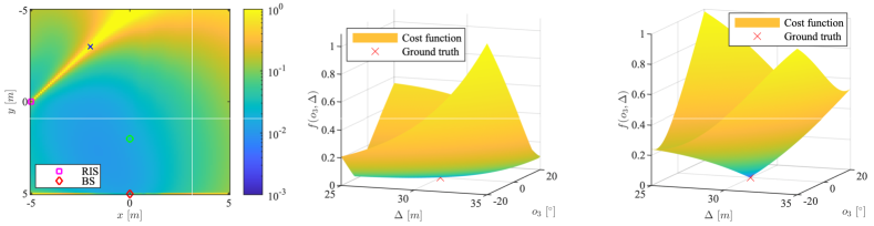
                              (a)                                                  (b)                                                       (c)

Figure 9: The visualization of the blind areas. (a) $\mathrm{EB}(\mathbf{p}_{\text{U}})$ versus $\mathbf{p}_{\text{U}}$, where the geometries of the bs and the ris are fixed as in Table I. In addition, two sample locations of the blind area (blue cross) and non-blind area (green circle) are shown; (b) $f(o_{3},\Delta)$ of the blind location in (a); (c) $f(o_{3},\Delta)$ of the non-blind location in (a).

So far we have presented results for scenarios with fixed ue and ris positions and orientations. In this subsection, we examine the spatial variability of performance. To this end, the localization crlb (take $\mathrm{EB}(\mathbf{p}_{\text{U}})$ as a representative) are computed over different ue positions while the bs and ris positions and orientations are kept fixed. We assume the ue to be placed across a $10\,\mathrm{m}\times 10\,\mathrm{m}$ space at a fixed height of 1 m, and the bs and ris are deployed as default parameters in Table I. The corresponding results are shown in Fig. 9 (a). From Fig. 9 (a), we can observe the presence of areas with extremely high crlb (yellow areas). Since these areas with high crlb yield a poor localization performance or are even unable to perform localization because of the existence of the ambiguity [27], we name those areas as the blind areas. In Fig. 9 (a), we select two sample locations of the blind area (blue cross) and non-blind area (green circle), respectively, for further investigation.

Fig. 9 (b) and (c) visualize the cost function $f({o}_{3},{\Delta})$ in (67) with the noise-free observations $\bm{\eta}$ for the selected blind and non-blind locations of the ue as marked in Fig. 9 (a). The ground-truth values of ${o}_{3}$ and ${\Delta}$ are marked with a red cross. In both cases, we can see that the ground truth coincides with a local minimum point, which indicates that Algorithm 2 can converge to the ground truth given a proper initialization search of the interval. However, the cost function of the blind location is flat around the ground truth, while the non-blind location shows a sharper descending structure. This implies that the uncertainty in the blind location is much higher than that in the non-blind location, and so the blind locations would produce a larger estimation error than the non-blind locations in the noisy case, which results in the extremely high crlb in Fig. 9 (a). To avoid localization in blind areas, we propose two strategies, namely, leveraging more prior information and adding extra bs.

VI-D2 Evaluation of the Impact of Extra Prior Information

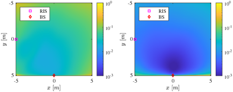
(a)                                    (b)

Figure 10: $\mathrm{EB}(\mathbf{p}_{\text{U}})$ versus $\mathbf{p}_{\text{U}}$. (a) The ris’s orientation $o_{3}$ is known; (b) The clock bias $\Delta$ is known.

We first assess the impact of using extra prior information on unknown localization parameters. We test two types of prior information, i.e., the ris’s orientation $o_{3}$ and the clock bias $\Delta$. Assume that we know the values of these two parameters in advance. Then, we remove the corresponding columns in the Jacobian matrix $\mathbf{J}$ in (81) and calculate a new crlb accordingly. The results are shown in Fig. 10. It can be seen that with prior knowledge of $o_{3}$ or $\Delta$, the blind area is greatly reduced. Furthermore, prior knowledge of $\Delta$ seems to provide a better performance in eliminating the blind area effect compared to using $o_{3}$. This can be explained by the fact that $\Delta$ contains more information than $o_{3}$ regarding the geometry of the ue and the ris. For example, once we know the clock bias $\Delta$, we can determine the positions of the ue and the ris immediately through (64)–(66), while the ris orientation $o_{3}$ cannot provide further information other than itself.

VI-D3 Evaluation of the Impact of Additional bs

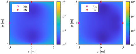
(a)                                    (b)

Figure 11: $\mathrm{EB}(\mathbf{p}_{\text{U}})$ versus $\mathbf{p}_{\text{U}}$. (a) Add one bs at $[0,-5,3]^{\mathsf{T}}$ with orientation $[0,0,\pi/2]^{\mathsf{T}}$; (b) Add two bs at $\{[0,-5,3]^{\mathsf{T}},[5,0,3]^{\mathsf{T}}\}$ with orientation $\{[0,0,\pi/2]^{\mathsf{T}},[0,0,\pi]^{\mathsf{T}}\}$.

Finally, we evaluate the impact of adding more bs. Fig. 11 demonstrates the value of $\mathrm{EB}(\mathbf{p}_{\text{U}})$ for ue at different positions under different amount of bs. In Fig. 11 (a), an additional bs is introduced at $[0,-5,3]^{\mathsf{T}}$ with orientation $[0,0,\pi/2]^{\mathsf{T}}$, while one more bs is added at $[5,0,3]^{\mathsf{T}}$ with orientation $[0,0,\pi]^{\mathsf{T}}$ in Fig. 11 (b). For each case, we collect parallel observations $\mathbf{y}_{g,k}$ from multiple bs, which is dependent on the same geometric parameters of the ue and the ris. Then the crlb are rederived and evaluated. We can observe that adding more bs can significantly reduce the blind areas. The more bs we deploy, the lower the overall localization bounds.

VII Conclusion

In this paper, we formulated and solved a joint ris calibration and user positioning problem for an active RIS-assisted uplink simo system, where the 3D user position, 3D RIS position, 1D RIS orientation, and clock bias were estimated. A two-stage localization method has been proposed, which consists of a coarse channel parameter estimation using tensor-esprit, a channel parameters refinement via ls estimation, and a 2d search-based localization algorithm. The fundamental crlb for the channel parameter and localization parameter estimation were derived. Through simulation studies, we demonstrated the effectiveness of the proposed algorithms by comparing their estimation rmse with those of the existing SOMP algorithm and the derived crlb. In addition, a comparison between the performance of the active and passive ris was carried out, which showed that active ris outperform the passive riss in terms of localization accuracy within practical power supply regions. Furthermore, we show that blind areas exist in the jrcup problem, which can be interpreted by the uncertainty in the cost function. Two strategies are proposed to combat blind areas, namely, using additional prior information (e.g., from extra sensors) or deploying more bs. These strategies have been verified by numerical simulations. Future research on the jrcup problem includes extending the formulation to multi-user/multi-ris scenarios, addressing 3d ris orientation estimation, as well as developing the ris mutual coupling-aware estimators.

Appendix A

Consider estimating the deterministic unknowns $\mathbf{x}\in\mathbb{R}^{l}$ from $\tilde{\mathbf{y}}\in\mathbb{C}^{m}$ based on the noisy observation model

$$\tilde{\mathbf{y}}=\tilde{\mathbf{f}}(\mathbf{x})+\tilde{\mathbf{A}}\tilde{\mathbf{n}},$$ (88)

where $\tilde{\mathbf{A}}\in\mathbf{C}^{m\times n}$, $\tilde{\mathbf{n}}\in\mathbb{C}^{n}$ and $\tilde{\mathbf{n}}\sim\mathcal{C}\mathcal{N}(\mathbf{0},\sigma^{2}\mathbf{I}_{n})$. Suppose $\tilde{\mathbf{y}}=\mathbf{y}_{\mathrm{R}}+j\mathbf{y}_{\mathrm{I}}$, $\tilde{\mathbf{f}}(\mathbf{x})=\mathbf{f}_{\mathrm{R}}(\mathbf{x})+j\mathbf{f}_{\mathrm{I}}(\mathbf{x})$, $\tilde{\mathbf{A}}=\mathbf{A}_{\mathrm{R}}+j\mathbf{A}_{\mathrm{I}}$ and $\tilde{\mathbf{n}}=\mathbf{n}_{\mathrm{R}}+j\mathbf{n}_{\mathrm{I}}$. By separating the real and imaginary parts of the observations $\tilde{\mathbf{y}}$, we can rewrite the model (88) as

$$\begin{bmatrix}\mathbf{y}_{\mathrm{R}}\\ \mathbf{y}_{\mathrm{I}}\end{bmatrix}=\underbrace{\begin{bmatrix}\mathbf{f}_{\mathrm{R}}(\mathbf{x})\\ \mathbf{f}_{\mathrm{I}}(\mathbf{x})\end{bmatrix}}_{\mathbf{f}(\mathbf{x})}+\underbrace{\begin{bmatrix}\mathbf{A}_{\mathrm{R}}\mathbf{n}_{\mathrm{R}}-\mathbf{A}_{\mathrm{I}}\mathbf{n}_{\mathrm{I}}\\ \mathbf{A}_{\mathrm{R}}\mathbf{n}_{\mathrm{I}}+\mathbf{A}_{\mathrm{I}}\mathbf{n}_{\mathrm{R}}\end{bmatrix}}_{\mathbf{n}}.$$ (89)

Since

$$\mathbf{A}_{\mathrm{R}}\mathbf{n}_{\mathrm{R}}-\mathbf{A}_{\mathrm{I}}\mathbf{n}_{\mathrm{I}}\sim\mathcal{N}\Big{(}\mathbf{0},\frac{\sigma^{2}}{2}(\mathbf{A}_{\mathrm{R}}\mathbf{A}_{\mathrm{R}}^{\mathsf{T}}+\mathbf{A}_{\mathrm{I}}\mathbf{A}_{\mathrm{I}}^{\mathsf{T}})\Big{)},$$ (90)

$$\mathbf{A}_{\mathrm{R}}\mathbf{n}_{\mathrm{I}}+\mathbf{A}_{\mathrm{I}}\mathbf{n}_{\mathrm{R}}\sim\mathcal{N}\Big{(}\mathbf{0},\frac{\sigma^{2}}{2}(\underbrace{\mathbf{A}_{\mathrm{R}}\mathbf{A}_{\mathrm{R}}^{\mathsf{T}}+\mathbf{A}_{\mathrm{I}}\mathbf{A}_{\mathrm{I}}^{\mathsf{T}}}_{=\mathfrak{R}(\tilde{\mathbf{A}}\tilde{\mathbf{A}}^{\mathsf{H}})})\Big{)},$$ (91)

and

$$\mathbb{E}\left[(\mathbf{A}_{\mathrm{R}}\mathbf{n}_{\mathrm{R}}-\mathbf{A}_{\mathrm{I}}\mathbf{n}_{\mathrm{I}})(\mathbf{A}_{\mathrm{R}}\mathbf{n}_{\mathrm{I}}+\mathbf{A}_{\mathrm{I}}\mathbf{n}_{\mathrm{R}})^{\mathsf{T}}\right]$$

$$= \frac{\sigma^{2}}{2}(\mathbf{A}_{\mathrm{R}}\mathbf{A}_{\mathrm{I}}^{\mathsf{T}}-\mathbf{A}_{\mathrm{I}}\mathbf{A}_{\mathrm{R}}^{\mathsf{T}})=\frac{\sigma^{2}}{2}\mathfrak{I}(\tilde{\mathbf{A}}\tilde{\mathbf{A}}^{\mathsf{H}})^{\mathsf{T}},$$ (92)

we have

$$\mathbf{n}\sim\mathcal{N}\Bigg{(}\mathbf{0},\underbrace{\frac{\sigma^{2}}{2}\begin{bmatrix}\mathfrak{R}\left(\mathbf{A}\mathbf{A}^{\mathsf{H}}\right)&\mathfrak{I}\left(\mathbf{A}\mathbf{A}^{\mathsf{H}}\right)^{\mathsf{T}}\vspace{0.3em}\\ \mathfrak{I}\left(\mathbf{A}\mathbf{A}^{\mathsf{H}}\right)&\mathfrak{R}\left(\mathbf{A}\mathbf{A}^{\mathsf{H}}\right)\end{bmatrix}}_{\mathbf{C}_{n}}\Bigg{)}.$$ (93)

Then the fim of $\mathbf{x}$ can be derived as [49, B.3.3]

$$\mathbf{J}(\mathbf{x})=\begin{bmatrix}\mathfrak{R}(\frac{\partial\tilde{\mathbf{f}}(\mathbf{x})}{\partial\mathbf{x}})\\ \mathfrak{I}(\frac{\partial\tilde{\mathbf{f}}(\mathbf{x})}{\partial\mathbf{x}})\end{bmatrix}^{\mathsf{T}}\mathbf{C}_{n}^{-1}\begin{bmatrix}\mathfrak{R}(\frac{\partial\tilde{\mathbf{f}}(\mathbf{x})}{\partial\mathbf{x}})\\ \mathfrak{I}(\frac{\partial\tilde{\mathbf{f}}(\mathbf{x})}{\partial\mathbf{x}})\end{bmatrix}.$$ (94)

Letting $\mathbf{A}_{0}=\mathbf{W}^{\mathsf{H}}$, $\mathbf{A}_{r}^{g,k}=\mathbf{W}^{\mathsf{H}}\mathbf{H}_{\text{R},2}^{k}\bm{\Gamma}_{g}$ and adding up the fim over all the transmissions $g=1,\dots,G$ and subcarriers $k=1,\dots,K$ yield Proposition 2.

References

• [1] Y. Liu, X. Liu, X. Mu, T. Hou, J. Xu, M. Di Renzo, and N. Al-Dhahir, “Reconfigurable intelligent surfaces: Principles and opportunities,” IEEE Communications Surveys & Tutorials, vol. 23, no. 3, pp. 1546–1577, 2021.
• [2] C. Pan, G. Zhou, K. Zhi, S. Hong, T. Wu, Y. Pan, H. Ren, M. D. Renzo, A. Lee Swindlehurst, R. Zhang, and A. Y. Zhang, “An overview of signal processing techniques for RIS/IRS-Aided wireless systems,” IEEE Journal of Selected Topics in Signal Processing, vol. 16, no. 5, pp. 883–917, 2022.
• [3] J. He, F. Jiang, K. Keykhosravi, J. Kokkoniemi, H. Wymeersch, and M. Juntti, “Beyond 5G RIS mmWave systems: Where communication and localization meet,” IEEE Access, vol. 10, pp. 68 075–68 084, 2022.
• [4] H. Sarieddeen, M.-S. Alouini, and T. Y. Al-Naffouri, “An overview of signal processing techniques for terahertz communications,” Proceedings of the IEEE, vol. 109, no. 10, pp. 1628–1665, 2021.
• [5] H. Chen, H. Sarieddeen, T. Ballal, H. Wymeersch, M.-S. Alouini, and T. Y. Al-Naffouri, “A tutorial on terahertz-band localization for 6G communication systems,” IEEE Communications Surveys & Tutorials, vol. 24, no. 3, pp. 1780–1815, 2022.
• [6] Z. Zhang, L. Dai, X. Chen, C. Liu, F. Yang, R. Schober, and H. Vincent Poor, “Active RIS vs. passive RIS: Which will prevail in 6G?” IEEE Transactions on Communications, vol. 71, no. 3, pp. 1707–1725, 2023.
• [7] R. Schroeder, J. He, G. Brante, and M. Juntti, “Two-stage channel estimation for hybrid RIS assisted MIMO systems,” IEEE Transactions on Communications, vol. 70, no. 7, pp. 4793–4806, 2022.
• [8] X. Mu, Y. Liu, L. Guo, J. Lin, and R. Schober, “Simultaneously transmitting and reflecting (STAR) RIS aided wireless communications,” IEEE Transactions on Wireless Communications, vol. 21, no. 5, pp. 3083–3098, 2022.
• [9] J. A. del Peral-Rosado, R. Raulefs, J. A. López-Salcedo, and G. Seco-Granados, “Survey of cellular mobile radio localization methods: From 1G to 5G,” IEEE Communications Surveys & Tutorials, vol. 20, no. 2, pp. 1124–1148, 2018.
• [10] P. Zheng, X. Liu, T. Ballal, and T. Y. Al-Naffouri, “5G-aided RTK positioning in GNSS-deprived environments,” in IEEE European Signal Processing Conference (EUSIPCO), 2023.
• [11] X. Fang, X. Li, and L. Xie, “3-D distributed localization with mixed local relative measurements,” IEEE Transactions on Signal Processing, vol. 68, pp. 5869–5881, 2020.
• [12] E. Björnson, H. Wymeersch, B. Matthiesen, P. Popovski, L. Sanguinetti, and E. de Carvalho, “Reconfigurable intelligent surfaces: A signal processing perspective with wireless applications,” IEEE Signal Processing Magazine, vol. 39, no. 2, pp. 135–158, 2022.
• [13] H. Chen, H. Kim, M. Ammous, G. Seco-Granados, G. C. Alexandropoulos, S. Valaee, and H. Wymeersch, “RISs and sidelink communications in smart cities: The key to seamless localization and sensing,” accepted by IEEE Communications Magazine, 2023.
• [14] H. Kim, H. Chen, M. F. Keskin, Y. Ge, K. Keykhosravi, G. C. Alexandropoulos, S. Kim, and H. Wymeersch, “RIS-enabled and access-point-free simultaneous radio localization and mapping,” preprint arXiv:2212.07141, 2022.
• [15] H. Chen, P. Zheng, M. F. Keskin, T. Al-Naffouri, and H. Wymeersch, “Multi-RIS-enabled 3D sidelink positioning,” preprint arXiv:2302.12459, 2023.
• [16] K. Keykhosravi, M. F. Keskin, G. Seco-Granados, P. Popovski, and H. Wymeersch, “RIS-Enabled SISO localization under user mobility and spatial-wideband effects,” IEEE Journal of Selected Topics in Signal Processing, vol. 16, no. 5, pp. 1125–1140, 2022.
• [17] J. He, A. Fakhreddine, and G. C. Alexandropoulos, “Simultaneous indoor and outdoor 3D localization with STAR-RIS-assisted millimeter wave systems,” in IEEE Vehicular Technology Conference (VTC), 2022.
• [18] H. Zhang, H. Zhang, B. Di, K. Bian, Z. Han, and L. Song, “Metalocalization: Reconfigurable intelligent surface aided multi-user wireless indoor localization,” IEEE Transactions on Wireless Communications, vol. 20, no. 12, pp. 7743–7757, 2021.
• [19] A. Elzanaty, A. Guerra, F. Guidi, and M.-S. Alouini, “Reconfigurable intelligent surfaces for localization: Position and orientation error bounds,” IEEE Transactions on Signal Processing, vol. 69, pp. 5386–5402, 2021.
• [20] A. Fascista, M. F. Keskin, A. Coluccia, H. Wymeersch, and G. Seco-Granados, “RIS-aided joint localization and synchronization with a single-antenna receiver: Beamforming design and low-complexity estimation,” IEEE Journal of Selected Topics in Signal Processing, vol. 16, no. 5, pp. 1141–1156, 2022.
• [21] P. Gao, L. Lian, and J. Yu, “Wireless area positioning in RIS-Assisted mmWave systems: Joint passive and active beamforming design,” IEEE Signal Processing Letters, vol. 29, pp. 1372–1376, 2022.
• [22] M. F. Keskin, F. Jiang, F. Munier, G. Seco-Granados, and H. Wymeersch, “Optimal spatial signal design for mmWave positioning under imperfect synchronization,” IEEE Transactions on Vehicular Technology, vol. 71, no. 5, pp. 5558–5563, 2022.
• [23] P. Zheng, H. Chen, T. Ballal, H. Wymeersch, and T. Y. Al-Naffouri, “Misspecified Cramér-Rao bound of RIS-aided localization under geometry mismatch,” in IEEE International Conference on Acoustics, Speech, & Signal Processing (ICASSP), 2023.
• [24] D.-R. Emenonye, H. S. Dhillon, and R. M. Buehrer, “RIS-Aided localization under position and orientation offsets in the near and far field,” preprint arXiv:2210.03599, 2022.
• [25] M. Samir, M. Elhattab, C. Assi, S. Sharafeddine, and A. Ghrayeb, “Optimizing age of information through aerial reconfigurable intelligent surfaces: A deep reinforcement learning approach,” IEEE Transactions on Vehicular Technology, vol. 70, no. 4, pp. 3978–3983, 2021.
• [26] L. Ge, H. Zhang, J.-B. Wang, and G. Y. Li, “Reconfigurable wireless relaying with Multi-UAV-carried intelligent reflecting surfaces,” IEEE Transactions on Vehicular Technology, vol. 72, no. 4, pp. 4932–4947, 2023.
• [27] Y. Lu, H. Chen, J. Talvitie, H. Wymeersch, and M. Valkama, “Joint RIS calibration and multi-user positioning,” in IEEE Vehicular Technology Conference (VTC), 2022.
• [28] R. Ghazalian, H. Chen, G. C. Alexandropoulos, G. Seco-Granados, H. Wymeersch, and R. Jäntti, “Joint user localization and location calibration of a hybrid reconfigurable intelligent surface,” preprint arXiv:2210.10150, 2022.
• [29] G. Mylonopoulos, C. D’Andrea, and S. Buzzi, “Active reconfigurable intelligent surfaces for user localization in mmWave MIMO systems,” in IEEE International Workshop on Signal Processing Advances in Wireless Communications (SPAWC), 2022.
• [30] G. Mylonopoulos, L. Venturino, S. Buzzi, and C. D’Andrea, “Maximum-likelihood user localization in active-RIS empowered mmWave wireless networks,” in 17th European Conference on Antennas and Propagation, 2023.
• [31] S. Abeywickrama, R. Zhang, Q. Wu, and C. Yuen, “Intelligent reflecting surface: Practical phase shift model and beamforming optimization,” IEEE Transactions on Communications, vol. 68, no. 9, pp. 5849–5863, 2020.
• [32] R. Long, Y.-C. Liang, Y. Pei, and E. G. Larsson, “Active reconfigurable intelligent surface-aided wireless communications,” IEEE Transactions on Wireless Communications, vol. 20, no. 8, pp. 4962–4975, 2021.
• [33] J. Rao, Y. Zhang, S. Tang, Z. Li, C.-Y. Chiu, and R. Murch, “An active reconfigurable intelligent surface utilizing phase-reconfigurable reflection amplifiers,” IEEE Transactions on Microwave Theory and Techniques, vol. 71, no. 7, pp. 3189–3202, 2023.
• [34] Z. Peng, X. Liu, C. Pan, L. Li, and J. Wang, “Multi-pair D2D communications aided by an active RIS over spatially correlated channels with phase noise,” IEEE Wireless Communications Letters, vol. 11, no. 10, pp. 2090–2094, 2022.
• [35] S. Saab, A. Mezghani, and R. W. Heath, “Optimizing the mutual information of frequency-selective multi-port antenna arrays in the presence of mutual coupling,” IEEE Transactions on Communications, vol. 70, no. 3, pp. 2072–2084, 2022.
• [36] M. Di Renzo, F. H. Danufane, and S. Tretyakov, “Communication models for reconfigurable intelligent surfaces: From surface electromagnetics to wireless networks optimization,” Proceedings of the IEEE, vol. 110, no. 9, pp. 1164–1209, 2022.
• [37] Y. Mitikiri and K. Mohseni, “Acceleration compensation for gravity sense using an accelerometer in an aerodynamically stable UAV,” in IEEE Conference on Decision and Control, 2019, pp. 1177–1182.
• [38] A. Cichocki, D. Mandic, L. De Lathauwer, G. Zhou, Q. Zhao, C. Caiafa, and H. A. PHAN, “Tensor decompositions for signal processing applications: From two-way to multiway component analysis,” IEEE Signal Processing Magazine, vol. 32, no. 2, pp. 145–163, 2015.
• [39] N. D. Sidiropoulos, L. De Lathauwer, X. Fu, K. Huang, E. E. Papalexakis, and C. Faloutsos, “Tensor decomposition for signal processing and machine learning,” IEEE Transactions on Signal Processing, vol. 65, no. 13, pp. 3551–3582, 2017.
• [40] M. Haardt, F. Roemer, and G. Del Galdo, “Higher-order SVD-Based subspace estimation to improve the parameter estimation accuracy in multidimensional harmonic retrieval problems,” IEEE Transactions on Signal Processing, vol. 56, no. 7, pp. 3198–3213, 2008.
• [41] R. Roy and T. Kailath, “ESPRIT-estimation of signal parameters via rotational invariance techniques,” IEEE Transactions on acoustics, speech, and signal processing, vol. 37, no. 7, pp. 984–995, 1989.
• [42] J. Zhang, D. Rakhimov, and M. Haardt, “Gridless channel estimation for hybrid mmWave MIMO systems via Tensor-ESPRIT algorithms in DFT beamspace,” IEEE Journal of Selected Topics in Signal Processing, vol. 15, no. 3, pp. 816–831, 2021.
• [43] S. Jiang, N. Fu, Z. Wei, X. Li, L. Qiao, and X. Peng, “Joint spectrum, carrier, and DOA estimation with beamforming MWC sampling system,” IEEE Transactions on Instrumentation and Measurement, vol. 71, pp. 1–15, 2022.
• [44] N. Fu, Z. Wei, L. Qiao, and Z. Yan, “Short-observation measurement of multiple sinusoids with multichannel sub-Nyquist sampling,” IEEE Transactions on Instrumentation and Measurement, vol. 69, no. 9, pp. 6853–6869, 2020.
• [45] T. G. Kolda and B. W. Bader, “Tensor decompositions and applications,” SIAM review, vol. 51, no. 3, pp. 455–500, 2009.
• [46] F. Wen, H. C. So, and H. Wymeersch, “Tensor decomposition-based beamspace ESPRIT algorithm for multidimensional harmonic retrieval,” in IEEE International Conference on Acoustics, Speech, & Signal Processing (ICASSP), 2020, pp. 4572–4576.
• [47] F. Jiang, F. Wen, Y. Ge, M. Zhu, H. Wymeersch, and F. Tufvesson, “Beamspace multidimensional ESPRIT approaches for simultaneous localization and communications,” preprint arXiv:2111.07450, 2021.
• [48] F. Wen, N. Garcia, J. Kulmer, K. Witrisal, and H. Wymeersch, “Tensor decomposition based beamspace ESPRIT for millimeter wave MIMO channel estimation,” in IEEE Global Communications Conference (GLOBECOM), 2018.
• [49] P. Stoica, R. L. Moses et al., Spectral analysis of signals.   Pearson Prentice Hall Upper Saddle River, NJ, 2005, vol. 452.
• [50] S. M. Kay, Fundamentals of statistical signal processing: estimation theory.   Prentice-Hall, Inc., 1993.
• [51] S. Tarboush, A. Ali, and T. Y. Al-Naffouri, “Compressive estimation of near field channels for ultra massive-MIMO wideband THz systems,” in IEEE International Conference on Acoustics, Speech, & Signal Processing (ICASSP), 2023.
• [52] ——, “Cross-field channel estimation for ultra massive-MIMO THz systems,” preprint arXiv:2305.13757, 2023.
• [53] E. J. Candes and T. Tao, “Near-optimal signal recovery from random projections: Universal encoding strategies?” IEEE Transactions on Information Theory, vol. 52, no. 12, pp. 5406–5425, 2006.
• [54] N. Boumal, B. Mishra, P.-A. Absil, and R. Sepulchre, “Manopt, a Matlab toolbox for optimization on manifolds,” Journal of Machine Learning Research, vol. 15, no. 42, pp. 1455–1459, 2014. [Online]. Available: https://www.manopt.org
• [55] F. Athley, “Threshold region performance of maximum likelihood direction of arrival estimators,” IEEE Transactions on Signal Processing, vol. 53, no. 4, pp. 1359–1373, 2005.
• [56] S. Shen, B. Clerckx, and R. Murch, “Modeling and architecture design of reconfigurable intelligent surfaces using scattering parameter network analysis,” IEEE Transactions on Wireless Communications, vol. 21, no. 2, pp. 1229–1243, 2022.
• [57] D. Wijekoon, A. Mezghani, and E. Hossain, “Beamforming optimization in RIS-aided MIMO systems under multiple-reflection effects,” in IEEE International Conference on Acoustics, Speech, & Signal Processing (ICASSP), 2023.
• [58] D. M. Pozar, Microwave engineering.   John wiley & sons, 2011.
• [59] M. Di Renzo, V. Galdi, and G. Castaldi, “Modeling the mutual coupling of reconfigurable metasurfaces,” in 17th European Conference on Antennas and Propagation, 2023.
• [60] P. Zheng, X. Ma, and T. Y. Al-Naffouri, “On the impact of mutual coupling on RIS-assisted channel estimation,” preprint arXiv:2309.04990, 2023.
• [61] X. Qian and M. D. Renzo, “Mutual coupling and unit cell aware optimization for reconfigurable intelligent surfaces,” IEEE Wireless Communications Letters, vol. 10, no. 6, pp. 1183–1187, 2021.