Multivariate probability distribution for categorical and ordinal random variables

Abstract

We propose a multivariate probability distribution for categorical and ordinal random variables. To this end, we use the Grassmann distribution in conjunction with dummy encoding of categorical and ordinal variables. To realize the co-occurrence probabilities of dummy variables required for categorical and ordinal variables, we propose a parsimonious parameterization for the Grassmann distribution that ensures the positivity of probability distribution. As an application of the proposed distribution, we develop a factor analysis for categorical and ordinal variables and show the validity of the model using a real dataset.

I Introduction

In data analysis, qualitative data such as categorical and ordinal variables often appear. Examples include demographic attributes such as gender and occupation, questionnaire responses in the Likert scale Likert (1932), and the presence of mutations in DNA and amino acid sequences. When qualitative variables appear as objective variables, multiclass logistic regression or probit regression can be applied Murphy (2012), however, it is difficult to construct a probabilistic generative model for qualitative variables. An example of a generative model for qualitative variables is a naive Bayes classifier using a categorical distribution Murphy (2012), but this model assumes independence between variables and cannot account for correlation. A possible method is to express correlation by latent variables, such as binary Factor Analysis (Tipping, 1998) and exponential family PCA (Collins et al., 2001; Mohamed et al., 2008). However, in general, introducing latent variables has the disadvantage that the induced probability distribution cannot be expressed analytically. This drawback causes difficulty in estimating the parameters of the model, and one has to resort to a computationally-demanding and time-consuming approximation technique. Therefore, dealing with qualitative data quantitatively is a challenging task.

The easiest way to handle multivariate categorical and ordinal variables is to treat them as continuous variables, ignoring their qualitative nature. For example, in questionnaire responses of the five-point scale, response variables, $\{1/5,2/5,\dots,1\}$, are treated as continuous numeric variables. Such treatment of qualitative variables is called methods of quantification. The quantification, however, treats variables of ordinal scale as ratio scale, that is, rudely assumes the intervals between ordinal responses as equally spaced. Hence the quantification has been criticized for being unreflective. One of the reasons that qualitative data are difficult to treat quantitatively stems from the fact that, unlike the continuous variables for which arithmetic operations can be defined, qualitative variables cannot be subjected to arithmetic operations such as addition, subtraction, multiplication, and division. Sensible analysis of qualitative data has often been limited to statistical testing of a contingency table, such as Fisher’s exact test or the Cochran-Armitage test. Therefore, in order to develop a sensible statistical model for qualitative data, a probability distribution that preserves the nature of the level of measurement is required.

Among categorical variables, multivariate binary random variables are represented by the Grassmann distribution Arai (2021). Also, recently, a probability distribution that models correlation between binary and continuous variables has been developed Arai (2022). The Grassmann distribution has nice theoretical properties similar to the multivariate normal distribution and has a computational advantage over the Ising model, a conventional multivariate Bernoulli distribution, in that there is no need to sum over all possible states explicitly when computing the partition function. This paper proposes a method to represent multivariate categorical and ordinal random variables using the Grassmann distribution in conjunction with the dummy encoding of categorical and ordinal variables.

This paper is organized as follows. In Sec. II, we summarize the proposed distribution and then explain the reasoning that the proposed distribution reproduces the co-occurrence probabilities of dummy variables required for categorical and ordinal variables. In Sec. III, we propose a parsimonious parametrization that enforces positive probabilities of the Grassmann distribution. This parametrization is a variant of the diagonally dominant parametrization and is necessary for the proposed distribution. In Sec. IV, we develop factor analysis for categorical and ordinal random variables as an application of the proposed probability distribution. The validity of the proposed factor analysis is demonstrated by analyzing a real dataset. A biplot visualization and its interpretation are given. Sec. V is devoted to conclusions.

II Proposed distribution

We first give a brief summary of the Grassmann distribution. It should be noted that the definition of the Grassmann distribution in this paper differs from the Grassmann distribution in the previous studies Arai (2021, 2022) in that the effect of dummy variables is inverted. This change of definition is intended to make the parameter matrix of the Grassmann distribution regular. Since the effect of the dummy variables is something like the definition of the sign (plus/minus) of the electric current, such a change is allowable, and it is not the essence of the problem. Therefore, we give a summary of the Grassmann distribution used in this paper, which is denoted by $\mathcal{G}^{(1)}$.

We denote $q$-dimensional dummy variables by a column vector $\mathbf{y}$, where each element takes the value $0$ or $1$. That is, the vector $\mathbf{y}$ is a bit vector with each element taking the value $0$ or $1$. We denote the set of whole indices of dummy variables as $R\equiv\{1,2,\dots,q\}$. An index label for dummy variables is divided into two parts with subscripts $1$ and $0$, for variables that take the value $1$ and $0$, respectively. For example, an index label for binary variables $R$ is divided into a subset $R_{1}\subseteq R$ and its set difference $R_{0}=R\setminus R_{1}$. Then, the joint distribution of the Grassmann distribution is expressed as follows:

$$p(\mathbf{y}_{R_{1}}=\bm{1},\mathbf{y}_{R_{0}}=\bm{0})= \mathcal{G}^{(1)}(\mathbf{y}_{R_{1}}=\bm{1},\mathbf{y}_{R_{0}}=\bm{0}\mid\Sigma),$$

$$= \det\begin{bmatrix}I-\Sigma_{R_{1}R_{1}}&\Sigma_{R_{1}R_{0}}\\ -\Sigma_{R_{0}R_{1}}&\Sigma_{R_{0}R_{0}}\end{bmatrix}=\frac{\det(\Lambda_{R_{1}R_{1}}-I)}{\det\Lambda},$$ (1)

where the indexed notation $\Sigma_{R_{1}R_{1}}$ expresses the submatrix of $\Sigma$, and $I$ is the identity matrix.

To express the marginal and conditional distributions, we first define the notation of index. We divide the sets of whole indices of dummy variables into two subset parts; $R=(S,T)$. The number of elements in these sets of indices is represented by $q_{S}$ and $q_{T}$, these of course satisfy $q_{S}+q_{T}=q$. Then, the subvector comprising the subset of indices $S$ is represented as $\mathbf{y}_{S}$. An index label for dummy variables is further divided into two parts with subscripts $1$ and $0$, for variables that take the value $1$ and $0$, respectively. For example, an index label for binary variables $S\subseteq R$ is divided into a subset $S_{1}\subseteq S$ and its set difference $S_{0}=S\setminus S_{1}$, where the subvectors $\mathbf{y}_{S_{1}}$ and $\mathbf{y}_{S_{0}}$ take the values as $\mathbf{y}_{S_{1}}=\bm{1}$ and $\mathbf{y}_{S_{0}}=\bm{0}$, respectively. Using the index notation described above, the marginal distribution is expressed as

$$p(\mathbf{y}_{T})=\mathcal{G}^{(1)}(\mathbf{y}_{T}\mid\Sigma_{TT}).$$ (2)

The conditional distribution is given by

$$p(\mathbf{y}_{S}\mid\mathbf{y}_{T})= \mathcal{G}^{(1)}(\mathbf{y}_{S}\mid\tilde{\Sigma}_{S|T}),$$ (3)

$$\tilde{\Sigma}= \begin{bmatrix}\tilde{\Sigma}_{SS}&\tilde{\Sigma}_{ST}\\ \tilde{\Sigma}_{TS}&\tilde{\Sigma}_{TT}\end{bmatrix}\equiv\begin{bmatrix}\Sigma_{SS}&-\Sigma_{ST_{1}}&\Sigma_{ST_{0}}\\ \Sigma_{T_{1}S}&I-\Sigma_{T_{1}T_{1}}&\Sigma_{T_{1}T_{0}}\\ \Sigma_{T_{0}S}&-\Sigma_{T_{0}T_{1}}&\Sigma_{T_{0}T_{0}}\end{bmatrix},$$ (4)

$$\tilde{\Sigma}_{S|T}\equiv \tilde{\Sigma}_{SS}-\tilde{\Sigma}_{ST}\tilde{\Sigma}_{TT}^{-1}\tilde{\Sigma}_{TS},$$

$$= [\Lambda_{SS}-\Lambda_{ST_{1}}(\Lambda_{T_{1}T_{1}}-I)^{-1}\Lambda_{T_{1}S}]^{-1},$$ (5)

where $\Sigma_{TT}^{-1}$ denotes the inverse matrix of the submatrix, $\Sigma_{TT}^{-1}\equiv(\Sigma_{TT})^{-1}$, and $\Sigma_{S|T}$ is the Schur complement.

The mean and covariance of dummy variables are given by

$$E[y_{r}]= 1-\Sigma_{rr},$$ (6)

$$\mathrm{Cov}[y_{r}\,y_{s}]= -\Sigma_{rs}\Sigma_{sr},\hskip 14.22636pt(r,s\in R).$$ (7)

That is, the diagonal element of $\Sigma$ expresses the marginal probability that the dummy variable takes the value of $0$. On the other hand, the conditional mean and covariance with all the other conditioned variables observed as $0$ are given by

$$E[y_{r}\mid\mathbf{y}_{R\setminus r}=\bm{0}]= 1-\frac{1}{\Lambda_{rr}}=\Bigl{(}\frac{\Lambda_{rr}}{\Lambda_{rr}-1}\Bigr{)}^{-1},$$ (8)

$$\mathrm{Cov}[y_{r}\,y_{s}\mid\mathbf{y}_{R\setminus\{r,s\}}=\bm{0}]= \frac{-\Lambda_{rs}\Lambda_{sr}}{(\Lambda_{rr}\Lambda_{ss}-\Lambda_{rs}\Lambda_{sr})^{2}}.$$ (9)

That is, the diagonal element of $\Lambda$ expresses the conditional probability that the dummy variable takes the value of $0$ with all the other conditioned variables observed as $0$.

The probability distribution that describes a correlation between continuous and dummy variables is summarized in Appendix A.

II.1 Statement of the result

First, we represent categorical and ordinal variables by dummy encoding.

For categorical variables, we use one-hot encoding; we represent a categorical variable with $(q_{C}+1)$ categories, $\delta\in\{0,1,2,\dots,q_{C}\}$, by using $q_{C}$ dummy variables, $y_{l}\in\{0,1\},\,(l=1,2,\dots,q_{C})$, each dummy variable is exclusively turned on. That is, we exclude a dummy variable for the base category. Table 2 shows an example of one-hot encoding with four categories.

For ordinal variables, we use dummy encoding similar to one-hot encoding. We represent an ordinal variable with $(q_{O}+1)$ levels, $\eta\in\{0,1,2,\dots,q_{O}\}$, by using $q_{O}$ dummy variables, $y_{l}\in\{0,1\},\,(l=1,2,\dots,q_{O})$, each dummy variable represents the flag meaning equal to or greater than one, two, etc. For example, the ordinal variable $\eta=2$ in the case of four levels can be expressed as $y_{1}=1$, $y_{2}=1$ and $y_{3}=0$, since it is greater than two and less than three. The dummy encoding for the case of four levels is shown in Table 2.

Note that in both the case of categorical and ordinal variables, a single dummy variable alone does not make sense, but the combination of multiple dummy variables makes sense. Binary variables can be treated as categorical variables with two categories, or as ordinal variables with two levels. We, therefore, treat binary variables as a special case of categorical variables.

Table 1: Categorical dummy variable.

$\delta$	$y_{1}$	$y_{2}$	$y_{3}$
$\delta=0$	0	0	0
$\delta=1$	1	0	0
$\delta=2$	0	1	0
$\delta=3$	0	0	1

Table 2: Ordinal dummy variable.

$\eta$	$y_{1}$	$y_{2}$	$y_{3}$
$\eta=0$	0	0	0
$\eta=1$	1	0	0
$\eta=2$	1	1	0
$\eta=3$	1	1	1

Let us consider the case where there are multiple categorical and ordinal variables. First, we define a notation to represent these variables collectively. We denote the number of categorical and ordinal variables as $c$ and $o$, respectively. The number of $j$th categorical variable $\delta_{j}$ is denoted by $q_{C_{j}}$. That is, the categorical variable $\delta_{j}$ takes the value in $\delta_{j}\in\{0,1,2,\dots,q_{C_{j}}\},\,(j=1,2,\dots,c)$. Similarly, the number of $j$th ordinal variable $\eta_{j}$ is denoted by $q_{O_{j}}$. That is, the ordinal variable $\eta_{j}$ takes the value in $\eta_{j}\in\{0,1,2,\dots,q_{O_{j}}\},\,(j=1,2,\dots,o)$. The categorical variable $\delta_{j}$ is encoded by the column vector of dummy variables $\mathbf{y}_{C_{j}}$, where $\mathbf{y}_{C_{j}}$ is a $q_{C_{j}}$-dimensional bit vector in which at most only one element can be turned on and all the other elements are zero. Similarly, the ordinal variable $\eta_{j}$ is encoded by the column vector of dummy variables $\mathbf{y}_{O_{j}}$, where

$$\mathbf{y}_{O_{j}}=[1,1,\dots,1,0,0,\dots,0]^{T}$$ (10)

is a $q_{O_{j}}$-dimensional bit vector in which all elements that take the value of one are flushed left. The dummy vectors of categorical and ordinal variables are combined into a single dummy vector $\mathbf{y}$,

$$\mathbf{y}=[\mathbf{y}_{C}^{T},\,\mathbf{y}_{O}^{T}]=[\mathbf{y}_{C_{1}}^{T},\,\mathbf{y}_{C_{2}}^{T},\,\dots,\,\mathbf{y}_{C_{c}}^{T},\,\mathbf{y}_{O_{1}}^{T},\,\mathbf{y}_{O_{2}}^{T},\,\dots,\,\mathbf{y}_{O_{o}}^{T}]^{T},$$ (11)

where the number of dimensions of the combined dummy vector $\mathbf{y}$ is $q=q_{C}+q_{O}\equiv q_{C_{1}}+q_{C_{2}}+\cdots+q_{C_{c}}+q_{O_{1}}+q_{O_{2}}+\cdots+q_{O_{o}}$. We denote the set of whole indices $\{1,2,\dots,q\}$ by $R$. Of the index set $R$, we denote the set of indices corresponding to categorical and ordinal variables as $C$ and $O$, respectively. These indices set satisfy $O=R\setminus C$. The set of these indices is partitioned into those of individual variables as $C=(C_{1},C_{2},\dots,C_{c})$ and $O=(O_{1},O_{2},\dots,O_{o})$.

The above categorical and ordinal dummy variables are modeled by the Grassmann distribution,

$$p(\mathbf{y})=\mathcal{G}^{(1)}(\mathbf{y}\mid\Sigma=\Lambda^{-1}),$$ (12)

where the parameters of the Grassmann distribution are represented by the following parsimonious expression:

$$\Lambda-I=\Psi^{-1}-I+W\Omega V^{T},$$ (13)

where $T$ stands for matrix transposition. The parameter $V$ is a $q\times a$ matrix, where the positive integer $a\in\{1,2,\dots,q\}$ represents the number of auxiliary latent dimensions and controls the representability of the model; larger values increase the representability of the model. $\Omega$ is a diagonal matrix of order $q$ whose diagonal elements take values between zero and one. The $q\times q$ matrix $\Psi$ must be a block-diagonal matrix such that each block element of $\Psi^{-1}-I$ is a quasi-diagonal matrix with nonnegative principal minors defined below from the requirement that certain co-occurrence probabilities of categorical and ordinal dummy variables be exactly zero:

$$\Psi^{-1}-I= \begin{bmatrix}(\Psi^{-1}-I)_{CC}&O\\ O&(\Psi^{-1}-I)_{OO}\end{bmatrix},$$ (14)

$$(\Psi^{-1}-I)_{CC}= \begin{bmatrix}(\Psi^{-1}-I)_{C_{1}C_{1}}&O&\cdots&O\\ O&(\Psi^{-1}-I)_{C_{2}C_{2}}&{}&\vdots\\ \vdots&{}&\ddots&O\\ O&\cdots&O&(\Psi^{-1}-I)_{C_{c}C_{c}}\end{bmatrix},$$ (15)

$$(\Psi^{-1}-I)_{C_{j}C_{j}}= \begin{bmatrix}(\bm{\psi}^{(C_{j})})^{T}\\ (\bm{\psi}^{(C_{j})})^{T}\\ \vdots\\ (\bm{\psi}^{(C_{j})})^{T}\end{bmatrix}=\begin{bmatrix}e^{b_{1}^{(C_{j})}}&e^{b_{2}^{(C_{j})}}&\cdots&e^{b_{q_{C_{j}}}^{(C_{j})}}\\ e^{b_{1}^{(C_{j})}}&e^{b_{2}^{(C_{j})}}&\cdots&e^{b_{q_{C_{j}}}^{(C_{j})}}\\ \vdots&\vdots&\cdots&\vdots\\ e^{b_{1}^{(C_{j})}}&e^{b_{2}^{(C_{j})}}&\cdots&e^{b_{q_{C_{j}}}^{(C_{j})}}\\ \end{bmatrix},\hskip 8.5359pt(j=1,2,\dots,c),$$ (16)

where $\bm{\psi}^{(C_{j})}$ and $\mathbf{b}^{(C_{j})}$ are $q_{C_{j}}$-dimensional column vectors, and

$$(\Psi^{-1}-I)_{OO}= \begin{bmatrix}(\Psi^{-1}-I)_{O_{1}O_{1}}&O&\cdots&O\\ O&(\Psi^{-1}-I)_{O_{2}O_{2}}&{}&\vdots\\ \vdots&{}&\ddots&O\\ O&\cdots&O&(\Psi^{-1}-I)_{O_{o}O_{o}}\end{bmatrix},$$ (18)

$$(\Psi^{-1}-I)_{O_{j}O_{j}}= L_{O_{j}}+\begin{bmatrix}\bm{\psi}^{(O_{j})},\;\;&\bm{0},\;\;&\dots,\;\;&\bm{0}\end{bmatrix}^{T},$$

$$= L_{O_{j}}+\begin{bmatrix}e^{b_{1}^{(O_{j})}}&e^{b_{1}^{(O_{j})}+b_{2}^{(O_{j})}}&\cdots&\prod_{l=1}^{q_{O_{j}}}e^{b_{l}^{(O_{j})}}\\ 0&0&\cdots&0\\ \vdots&\ddots&\ddots&\vdots\\ 0&\cdots&0&0\end{bmatrix},\hskip 8.5359pt(j=1,2,\dots,o),$$ (19)

where $\bm{\psi}^{(O_{j})}$ and $\mathbf{b}^{(O_{j})}$ are $q_{O_{j}}$-dimensional column vectors, and

$$L_{O_{j}}=\begin{bmatrix}0&0&0&\cdots&0\\ -1&0&0&\cdots&0\\ 0&-1&\ddots&\ddots&\vdots\\ \vdots&\ddots&\ddots&0&0\\ 0&0&0&-1&0\end{bmatrix}$$ (20)

is a lower triangular matrix of order $q_{O_{j}}$ with elements minus one. The $q\times a$ matrix $W$ must have the following form due to the requirement that the co-occurrence probabilities for categorical and ordinal dummy variables must be zero:

$$W= \begin{bmatrix}W_{CA}^{T},\;\;&W_{OA}^{T}\end{bmatrix}^{T},$$ (21)

$$W_{CA}= \begin{bmatrix}W_{C_{1}A}^{T},&W_{C_{2}A}^{T},&\dots,&W_{C_{c}A}^{T}\end{bmatrix}^{T},\hskip 2.84544ptW_{C_{j}A}=\begin{bmatrix}\mathbf{w}^{(C_{j})},&\mathbf{w}^{(C_{j})},&\dots,&\mathbf{w}^{(C_{j})}\end{bmatrix}^{T},\hskip 2.84544pt(j=1,2,\dots,c),$$ (22)

$$W_{OA}= \begin{bmatrix}W_{O_{1}A}^{T},&W_{O_{2}A}^{T},&\dots,&W_{O_{o}A}^{T}\end{bmatrix}^{T},\hskip 8.5359ptW_{O_{j}A}=\begin{bmatrix}\mathbf{w}^{(O_{j})},&\bm{0},&\dots,&\bm{0}\end{bmatrix}^{T},\hskip 8.5359pt(j=1,2,\dots,o),$$ (23)

where $W_{C_{j}A}$ is a $q_{C_{j}}\times a$ matrix and $\mathbf{w}^{(C_{j})}$ is an $a$-dimensional column vector. Also, $W_{O_{j}A}$ is a $q_{O_{j}}\times a$ matrix and $\mathbf{w}^{(O_{j})}$ is an $a$-dimensional column vector.

The Grassmann distribution is parametrized by the explicit model parameter $\theta_{m}=(\Psi,W,V,\Omega)$ as well as by an auxiliary parameter $\theta_{a}=(C)=(C_{RR},C_{RA},C_{AR},C_{AA})$. This auxiliary parameter does not affect the likelihood of the model directly. The $(q+a)\times(q+a)$ parameter matrix $C$ is block partitioned as follows:

$$C= \begin{bmatrix}C_{RR}&C_{RA}\\ C_{AR}&C_{AA}\end{bmatrix},$$ (24)

and must be a strictly diagonally dominant matrix. Also, the following matrix $B$, represented by the combination of model parameters, must be a diagonally dominant matrix:

$$B= \begin{bmatrix}B_{RR}&B_{RA}\\ B_{AR}&B_{AA}\end{bmatrix}=\begin{bmatrix}(\Psi^{-1}-I+WV^{T})C_{RR}-WC_{AR},\hskip 36.98866pt&(\Psi^{-1}-I+WV^{T})C_{RA}-WC_{AA}\\ C_{AR}-V^{T}C_{RR},&C_{AA}-V^{T}C_{RA}\end{bmatrix}.$$ (25)

These diagonally dominant and strictly diagonally dominant conditions are necessary for the parameter matrix of the Grassmann distribution $\Lambda-I$ to be a $P_{0}$-matrix. That is, the Grassmann distribution is parametrized by $\theta=(\theta_{m},\theta_{a})$.

II.2 Co-occurrence probabilities of dummy variables

It is not appropriate to model the categorical and ordinal dummy variables by the Grassmann distribution naively. This is because the probability of multiple dummies turning on at the same time, co-occurrence probabilities, can become nonzero in such a straightforward method. In this section, we explain how the parameterization of the Grassmann distribution in the previous section renders the undesired co-occurrence probabilities to exactly zero. In this paper, we sometimes refer to the probability that the dummy variable takes the value of one as excitation probability.

II.2.1 Excitation probabilities of categorical variable

In the one-hot encoding of categorical variables, multiple dummy variables do not turn on simultaneously, and at most one of the dummy variables turns on. Since the observation probability of dummy variables is expressed by the determinant of the parameter matrix $\tilde{\Sigma}$ as shown in Eq. (4), the matrix $\Sigma$ should be parametrized so that some row vectors of the parameter matrix coincide when multiple dummy variables are observed as one, in order to make the co-occurrence probability zero. In the specific example of four categories, the following parametrization realizes the desired excitation probabilities:

$$\Sigma=\begin{bmatrix}\Sigma_{11}&\Sigma_{22}-1&\Sigma_{33}-1\\ \Sigma_{11}-1&\Sigma_{22}&\Sigma_{33}-1\\ \Sigma_{11}-1&\Sigma_{22}-1&\Sigma_{33}\end{bmatrix},\hskip 14.22636pt\Lambda=\begin{bmatrix}\Lambda_{11}&\Lambda_{22}-1&\Lambda_{33}-1\\ \Lambda_{11}-1&\Lambda_{22}&\Lambda_{33}-1\\ \Lambda_{11}-1&\Lambda_{22}-1&\Lambda_{33}\end{bmatrix}.$$ (26)

In the above parametrization, only the four different excitation probabilities as represented in Table 2 become nonzero. These four probabilities can be expressed by the following categorical distribution:

$$p(\delta)= \mathrm{Cat}(\mathbf{y}|\mathbf{b})\equiv\frac{\exp(\mathbf{y}^{T}\mathbf{b})}{1+\sum_{l=1}^{q_{C}}\exp(b_{l})},\hskip 14.22636ptb_{l}=\log(\Lambda_{ll}-1).$$ (27)

II.2.2 Excitation probabilities of ordinal variable

In the dummy encoding of ordinal variables, the elements of the dummy vector that is turned on are flushed left as in Eq. (10). This means that the co-occurrence probability of the lower level of the dummy variable being zero while the upper level of the dummy variable is one must be exactly zero, e.g., $y_{l-1}=0$ and $y_{l}=1$ cannot occur simultaneously. Let us consider a specific example of four levels, i.e., $q_{O}=3$. The parametrization that enforces the aforementioned co-occurrence probabilities can be expressed as follows:

$$\Sigma=\begin{bmatrix}\Sigma_{11}&\Sigma_{22}-1&\Sigma_{33}-1\\ \Sigma_{11}&\Sigma_{22}&\Sigma_{33}-1\\ \Sigma_{11}&\Sigma_{22}&\Sigma_{33}\\ \end{bmatrix},\hskip 14.22636pt\Lambda=\begin{bmatrix}\Lambda_{11}&\Lambda_{12}&\Lambda_{13}\\ -1&1&0\\ 0&-1&1\end{bmatrix}.$$ (28)

In the above parametrization, only the four different excitation probabilities as represented in Table 2 become nonzero. These four probabilities are expressed by the ordinal distribution defined as follows:

$$p(\eta)= \mathrm{Ord}(\mathbf{y}|\mathbf{b})\equiv\frac{\exp(\mathbf{y}^{T}\mathbf{b})}{1+\sum_{l=1}^{q_{O}}\prod_{m=1}^{l}\exp(b_{m})},\hskip 11.38092pt\Lambda_{11}-1=e^{b_{1}},\hskip 5.69046pt\Lambda_{12}=e^{b_{1}+b_{2}},\hskip 5.69046pt\Lambda_{13}=e^{b_{1}+b_{2}+b_{3}}.$$ (29)

We shall call the matrices $\Lambda-I$ of the form as expressed in Eqs. (26, 28) a quasi-diagonal matrix with nonnegative principal minors.

II.2.3 Mixture of categorical and ordinal variables

When there is a mixture of a categorical variable and an ordinal variable with the number of levels four, the results of the previous section can be summarized in a block matrix as follows:

$$\Sigma= \begin{bmatrix}\Sigma_{CC}&\Sigma_{CO}\\ \Sigma_{OC}&\Sigma_{OO}\end{bmatrix}=\begin{bmatrix}\Sigma_{11}&\Sigma_{22}-1&\Sigma_{33}-1&\Sigma_{1O}\\ \Sigma_{11}-1&\Sigma_{22}&\Sigma_{33}-1&\Sigma_{1O}\\ \Sigma_{11}-1&\Sigma_{22}-1&\Sigma_{33}&\Sigma_{1O}\\ \Sigma_{O1}&\Sigma_{O2}&\Sigma_{O3}&\Sigma_{OO}\end{bmatrix}=\begin{bmatrix}\Sigma_{CC}&\Sigma_{C4}&\Sigma_{C5}&\Sigma_{C6}\\ \Sigma_{4C}&\Sigma_{44}&\Sigma_{55}-1&\Sigma_{66}-1\\ \Sigma_{4C}&\Sigma_{44}&\Sigma_{55}&\Sigma_{66}-1\\ \Sigma_{4C}&\Sigma_{44}&\Sigma_{55}&\Sigma_{66}\end{bmatrix},$$ (30)

$$\Lambda-I= \begin{bmatrix}\Lambda_{CC}-I&\Lambda_{CO}\\ \Lambda_{OC}&\Lambda_{OO}-I\end{bmatrix}=\begin{bmatrix}\Lambda_{11}-1&\Lambda_{22}-1&\Lambda_{33}-1&\Lambda_{1O}\\ \Lambda_{11}-1&\Lambda_{22}-1&\Lambda_{33}-1&\Lambda_{1O}\\ \Lambda_{11}-1&\Lambda_{22}-1&\Lambda_{33}-1&\Lambda_{1O}\\ \Lambda_{O1}&\Lambda_{O2}&\Lambda_{O3}&\Lambda_{OO}\end{bmatrix}=\begin{bmatrix}\Lambda_{CC}&\Lambda_{C4}&\Lambda_{C5}&\Lambda_{C6}\\ \Lambda_{4C}&\Lambda_{44}&\Lambda_{45}&\Lambda_{46}\\ \bm{0}^{T}&-1&0&0\\ \bm{0}^{T}&0&-1&0\end{bmatrix}.$$ (31)

The model parameter $\Lambda-I$ should be expressed as

$$\Lambda-I= \begin{bmatrix}(\Lambda-I)_{CR}\\ (\Lambda-I)_{OR}\end{bmatrix},\hskip 5.69046pt(\Lambda-I)_{CR}=\begin{bmatrix}(\bm{\lambda}^{(C)})^{T}\\ (\bm{\lambda}^{(C)})^{T}\\ (\bm{\lambda}^{(C)})^{T}\end{bmatrix},\hskip 5.69046pt(\Lambda-I)_{OR}=\begin{bmatrix}(\bm{\lambda}^{(O)})^{T}\\ \bm{0}^{T}\\ \bm{0}^{T}\end{bmatrix}+\begin{bmatrix}O,\;\;L\end{bmatrix},$$ (32)

where $O$ is a matrix with all elements zero, $L$ is the following lower triangular matrix,

$$L=\begin{bmatrix}0&0&0\\ -1&0&0\\ 0&-1&0\end{bmatrix},$$ (33)

and $\bm{\lambda}^{(C)}$ and $\bm{\lambda}^{(O)}$ are six-dimensional column vectors.

The case of multiple categorical and ordinal variables can also be represented using a block matrix. In fact, we see that $\Lambda-I$ can be parametrized as follows:

$$(\Lambda-I)_{CR}= \begin{bmatrix}(\Lambda-I)_{C_{1}R}\\ (\Lambda-I)_{C_{2}R}\\ \vdots\\ (\Lambda-I)_{C_{c}R}\end{bmatrix},\hskip 2.84544pt(\Lambda-I)_{C_{j}R}=\begin{bmatrix}(\bm{\lambda}^{(C_{j})})^{T}\\ (\bm{\lambda}^{(C_{j})})^{T}\\ \vdots\\ (\bm{\lambda}^{(C_{j})})^{T}\end{bmatrix},\hskip 8.5359pt(j=1,2,\dots,c),$$ (34)

$$(\Lambda-I)_{OR}= \begin{bmatrix}(\Lambda-I)_{O_{1}R}\\ (\Lambda-I)_{O_{2}R}\\ \vdots\\ (\Lambda-I)_{O_{o}R}\end{bmatrix}=\begin{bmatrix}(\Lambda-I)_{O_{1}C},&(\Lambda-I)_{O_{1}O}\\ (\Lambda-I)_{O_{2}C},&(\Lambda-I)_{O_{2}O}\\ \vdots,&\vdots\\ (\Lambda-I)_{O_{o}C},&(\Lambda-I)_{O_{o}O}\end{bmatrix}=\begin{bmatrix}\tilde{\Lambda}_{O_{1}R}\\ \tilde{\Lambda}_{O_{2}R}\\ \vdots\\ \tilde{\Lambda}_{O_{o}R}\end{bmatrix}+\begin{bmatrix}O&L_{O_{1}}&O&\cdots&O\\ O&O&L_{O_{2}}&\ddots&\vdots\\ \vdots&\vdots&\ddots&\ddots&O\\ O&O&\cdots&O&L_{O_{o}}\end{bmatrix},$$ (35)

$$\tilde{\Lambda}_{O_{j}R}= \begin{bmatrix}\bm{\lambda}^{(O_{j})},\;\;&\bm{0},\;\;&\dots,\;\;&\bm{0}\end{bmatrix}^{T},\hskip 8.5359pt(j=1,2,\dots,o),$$ (36)

where $L_{O_{j}}$ is a lower triangular matrix of order $q_{O_{j}}$ with elements minus zero as defined by Eq. (20).

III Parsimonious parametrization for Grassmann distribution

The parametrization of the Grassmann distribution in the previous section cannot be realized by the conventional diagonally dominant parametrization Arai (2021). Therefore, in this section, we propose a novel parsimonious parametrization for the Grassmann distribution.

III.1 Derivation of parsimonious parametrization

The parsimonious parametrization is a parametrization inspired by the idea of conventional factor analysis of continuous variables. We introduce the latent dimension of auxiliary dummy variables and represent the model parameter matrix, which should be a $P_{0}$-matrix, by a partitioned matrix. We denote the whole set of indices for observed dummy variables and latent dummy variables as $R$ and $A$, and also denote these dimensions as $q$ and $a$, respectively. The set of complete indices of observed and latent variables combined is denoted as $K=(R,A)$. Then, the matrix of model parameter $\Lambda-I$ with complete indices is defined by the product of the block upper triangular matrices as follows:

$$(\Lambda-I)_{KK}= \begin{bmatrix}I&O\\ O&(\Omega^{-1}-I)^{1/2}\end{bmatrix}\begin{bmatrix}\Psi^{-1}-I&-W\\ O&I\end{bmatrix}\begin{bmatrix}I&O\\ -V^{T}&I\end{bmatrix}\begin{bmatrix}I&O\\ O&(\Omega^{-1}-I)^{1/2}\end{bmatrix},$$

$$= \begin{bmatrix}I&O\\ O&(\Omega^{-1}-I)^{1/2}\end{bmatrix}\begin{bmatrix}\Psi^{-1}-I+WV^{T}&-W\\ -V^{T}&I\end{bmatrix}\begin{bmatrix}I&O\\ O&(\Omega^{-1}-I)^{1/2}\end{bmatrix},$$

$$= \begin{bmatrix}\Psi^{-1}-I+WV^{T},&-W(\Omega^{-1}-I)^{1/2}\\ -(\Omega^{-1}-I)^{1/2}V^{T}&\Omega^{-1}-I\end{bmatrix},$$ (37)

$$\Sigma_{KK}= \begin{bmatrix}\Lambda_{R|A}^{-1},&\Lambda_{R|A}^{-1}W\Omega^{1/2}(I-\Omega)^{1/2}\\ \Omega^{1/2}(I-\Omega)^{1/2}V^{T}\Lambda_{R|A}^{-1},&\Omega+\Omega^{1/2}(I-\Omega)^{1/2}V^{T}\Lambda_{R|A}^{-1}W\Omega^{1/2}(I-\Omega)^{1/2}\end{bmatrix},$$ (38)

$$\Lambda_{R|A}= \Psi^{-1}+W\Omega V^{T},$$ (39)

where $\Omega$ is a diagonal matrix with diagonal elements satisfying $0\leq\mathrm{diag}(\Omega)\leq 1$. $\Psi^{-1}-I$ is a block-diagonal matrix of quasi-diagonal matrices with nonnegative principal minors as defined in Sec. II.2, which is a square matrix that realizes the co-occurrence probabilities of categorical and ordinal dummy variables. In the above parametrization, conditional independence holds among observed variables as well as among latent variables. In fact, when the observed variables all take the value of one, the model parameter of the Grassmann distribution for latent variables conditioned on observed variables is given by $p(\mathbf{y}_{A}\mid\mathbf{y}_{R}=\bm{1})=\mathcal{G}^{(1)}(\mathbf{y}_{A}\mid\Omega)$, which means conditional independence among latent variables given observed variables. On the other hand, when the latent variables all take the value of zero, the model parameter of the Grassmann distribution for observed variables conditioned on latent variables is given by $p(\mathbf{y}_{R}\mid\mathbf{y}_{A}=\bm{0})=\mathcal{G}^{(1)}(\mathbf{y}_{R}\mid\Psi)$, which again means conditional independence among observed variables given latent variables.

A $P_{0}$-matrix is expressed by the product of row diagonally dominant matrices $B$ and $C$ of the form $BC^{-1}$ Tsatsomeros (2002). Since multiplying a nonnegative diagonal matrix does not change the $P_{0}$-matrix nature, we assume that the middle part of the right-hand side in Eq. (37) is decomposed to the product of row diagonally dominant matrix $B$ and strictly row diagonally dominant matrix $C$,

$$\begin{bmatrix}\Psi^{-1}-I+WV^{T}&-W\\ -V^{T}&I\end{bmatrix},$$

$$= \begin{bmatrix}B_{RR}&B_{RA}\\ B_{AR}&B_{AA}\end{bmatrix}\begin{bmatrix}C_{RR}&C_{RA}\\ C_{AR}&C_{AA}\end{bmatrix}^{-1},$$

$$= \begin{bmatrix}B_{RR}&B_{RA}\\ B_{AR}&B_{AA}\end{bmatrix}\begin{bmatrix}C_{RR}^{-1}+C_{RR}^{-1}C_{RA}C_{A|R}^{-1}C_{AR}C_{RR}^{-1},&-C_{RR}^{-1}C_{RA}C_{A|R}^{-1}\\ -C_{A|R}^{-1}C_{AR}C_{RR}^{-1},&C_{A|R}^{-1}\end{bmatrix},$$

$$= \begin{bmatrix}B_{RR}C_{RR}^{-1}-(B_{RA}-B_{RR}C_{RR}^{-1}C_{RA})C_{A|R}^{-1}C_{AR}C_{RR}^{-1},&(B_{RA}-B_{RR}C_{RR}^{-1}C_{RA})C_{A|R}^{-1}\\ B_{AR}C_{RR}^{-1}-(B_{AA}-B_{AR}C_{RR}^{-1}C_{RA})C_{A|R}^{-1}C_{AR}C_{RR}^{-1},&(B_{AA}-B_{AR}C_{RR}^{-1}C_{RA})C_{A|R}^{-1}\end{bmatrix}.$$ (40)

Comparing the $A$th column in the above equation, we see that the following two equations must hold,

$$\begin{cases}(B_{RA}-B_{RR}C_{RR}^{-1}C_{RA})=-WC_{A|R},\\ (B_{AA}-B_{AR}C_{RR}^{-1}C_{RA})=C_{A|R}.\end{cases}$$ (41)

Plugging the above equations into $R$th column in Eq. (40), we see the following two relations,

$$\begin{cases}B_{RR}C_{RR}^{-1}+WC_{AR}C_{RR}^{-1}=\Psi^{-1}-I+WV^{T},\\ B_{AR}C_{RR}^{-1}-C_{AR}C_{RR}^{-1}=-V^{T},\end{cases}\Rightarrow\begin{cases}B_{RR}C_{RR}^{-1}=\Psi^{-1}-I+WV^{T}-WC_{AR}C_{RR}^{-1},\\ B_{AR}C_{RR}^{-1}=C_{AR}C_{RR}^{-1}-V^{T}.\end{cases}$$ (42)

So, plugging the above expressions for $B_{RR}C_{RR}^{-1}$ and $B_{AR}C_{RR}^{-1}$ into Eq. (41), we obtain

$$\begin{cases}B_{RA}=(\Psi^{-1}-I+WV^{T})C_{RA}-WC_{AA},\\ B_{AA}=C_{AA}-V^{T}C_{RA}.\end{cases}$$ (43)

From the above calculus, the diagonally dominant matrix $B$ must have the following form,

$$B= \begin{bmatrix}(\Psi^{-1}-I+WV^{T})C_{RR}-WC_{AR},\hskip 36.98866pt&(\Psi^{-1}-I+WV^{T})C_{RA}-WC_{AA}\\ C_{AR}-V^{T}C_{RR},&C_{AA}-V^{T}C_{RA}\end{bmatrix}.$$ (44)

Marginalizing the latent variables, we obtain the parsimonious model parametrization of the Grassmann distribution for observed variables, $\theta=(\Psi,W,V,\Omega,C)$:

$$\Sigma_{RR}=[\Psi^{-1}+W\Omega V^{T}]^{-1},$$ (45)

with the row diagonally dominant condition for $B$, Eq. (44), and strictly row diagonally dominant condition for $C$.

III.2 Realization for categorical and ordinal parametrization

In the parsimonious parametrization of the Grassmann distribution, the model parameter $\Lambda-I$ is expressed as

$$\Lambda-I=\Psi^{-1}-I+W\Omega V^{T}.$$ (46)

We see that the parametrization required for categorical and ordinal variables as explained in Sec. II.2 can be realized by imposing the constraints on $\Psi$ and $W$.

III.2.1 Categorical variables only

Using the parsimonious parametrization, the parametrization for the categorical dummy variables in Sec. II.2.1,

$$\Lambda-I=\begin{bmatrix}\Lambda_{11}-1&\Lambda_{22}-1&\Lambda_{33}-1\\ \Lambda_{11}-1&\Lambda_{22}-1&\Lambda_{33}-1\\ \Lambda_{11}-1&\Lambda_{22}-1&\Lambda_{33}-1\end{bmatrix}=\Psi^{-1}-I+W\Omega V^{T},$$ (47)

can be realized by imposing constraints on $\Psi$ as $W$ as follows:

$$\Psi^{-1}-I=\begin{bmatrix}e^{b_{1}}&e^{b_{2}}&e^{b_{3}}\\ e^{b_{1}}&e^{b_{2}}&e^{b_{3}}\\ e^{b_{1}}&e^{b_{2}}&e^{b_{3}}\end{bmatrix},\hskip 14.22636ptW=\begin{bmatrix}\mathbf{w}^{T}\\ \mathbf{w}^{T}\\ \mathbf{w}^{T}\end{bmatrix},$$ (48)

where $\Psi^{-1}-I$ is a quasi-diagonal matrix with nonnegative principal minors, and $\mathbf{b}$ and $\mathbf{w}$ are three-dimensional column vectors.

III.2.2 Ordinal variable only

In a similar way, the parametrization for the ordinal dummy variables in Sec. II.2.2,

$$\Lambda-I=\begin{bmatrix}\Lambda_{11}-1&\Lambda_{12}&\Lambda_{13}\\ -1&0&0\\ 0&-1&0\end{bmatrix}=\Psi^{-1}-I+W\Omega V^{T},$$ (49)

can be realized by imposing constraints on $\Psi$ as $W$ as follows:

$$\Psi^{-1}-I=\begin{bmatrix}e^{b_{1}}&e^{b_{1}+b_{2}}&e^{b_{1}+b_{2}+b_{3}}\\ -1&0&0\\ 0&-1&0\end{bmatrix},\hskip 14.22636ptW=\begin{bmatrix}\mathbf{w}^{T}\\ \bm{0}^{T}\\ \bm{0}^{T}\end{bmatrix},$$ (50)

where $\Psi^{-1}-I$ is a quasi-diagonal matrix with nonnegative principal minors, and $\mathbf{b}$ and $\mathbf{w}$ are three-dimensional column vectors.

III.2.3 Mixture of categorical and ordinal variables

Parametrization for the case of a mixture of categorical and ordinal variables can be realized by representing $\Psi$ and $W$ in a partitioned matrix as follows:

$$\Lambda-I=\Psi^{-1}-I+W\Omega V^{T}=\begin{bmatrix}(\Psi^{-1}-I)_{CC}&O\\ O&(\Psi^{-1}-I)_{OO}\end{bmatrix}+\begin{bmatrix}W_{CA}\\ W_{OA}\end{bmatrix}\Omega V^{T}.$$ (51)

The parametrization for single categorical and ordinal variables each with the number of levels four can be realized by imposing constraints on $\Psi$ and $W$ as follows:

$$(\Psi^{-1}-I)_{CC}= \begin{bmatrix}(\bm{\psi}^{(C)})^{T}\\ (\bm{\psi}^{(C)})^{T}\\ (\bm{\psi}^{(C)})^{T}\end{bmatrix}=\begin{bmatrix}e^{b_{1}^{(C)}}&e^{b_{2}^{(C)}}&e^{b_{3}^{(C)}}\\ e^{b_{1}^{(C)}}&e^{b_{2}^{(C)}}&e^{b_{3}^{(C)}}\\ e^{b_{1}^{(C)}}&e^{b_{2}^{(C)}}&e^{b_{3}^{(C)}}\\ \end{bmatrix},$$ (52)

$$(\Psi^{-1}-I)_{OO}= L+\begin{bmatrix}(\bm{\psi}^{(O)})^{T}\\ \bm{0}^{T}\\ \bm{0}^{T}\end{bmatrix}=\begin{bmatrix}0&0&0\\ -1&0&0\\ 0&-1&0\end{bmatrix}+\begin{bmatrix}e^{b_{1}^{(O)}}&e^{b_{1}^{(O)}+b_{2}^{(O)}}&e^{b_{1}^{(O)}+b_{2}^{(O)}+b_{3}^{(O)}}\\ 0&0&0\\ 0&0&0\end{bmatrix},$$ (53)

$$W_{CA}= \begin{bmatrix}\mathbf{w}^{(C)},\;\;&\mathbf{w}^{(C)},\;\;&\mathbf{w}^{(C)}\end{bmatrix}^{T},\hskip 25.6073ptW_{OA}=\begin{bmatrix}\mathbf{w}^{(O)},\;\;&\bm{0},\;\;&\bm{0}\end{bmatrix}^{T}.$$ (54)

The case of multiple categorical and ordinal variables can be parametrized as in Sec. II.1.

III.3 Validation with real data

In this section, we numerically confirm that the proposed parsimonious parametrization successfully reproduces correlation and co-occurrence probabilities for categorical and ordinal dummy variables using a real dataset. The data used in this analysis is the reader data from catdata package of R (programming language) Gunther Schauberger (2020). The reader data contains information on the reading behavior of women referring to a specific woman’s journal and consists of four variables: is the woman a regular reader? ($\text{yes}=1,\,\text{no}=0$), is the woman working? ($\text{yes}=1,\,\text{no}=0$), their age group ($18\text{--}29:\text{years}=1,\,30\text{--}39:\text{years}=2,\,40\text{--}49:\text{years}=3$), and their education level from L1 to L4. The sample size of the dataset is $N=941$. We considered age group as a categorical variable and education level as an ordinal variable. We sampled one binary variable, Working, one categorical variable, Age category, and one ordinal variable, Education level, for analysis.

Model parameters were estimated by maximum likelihood estimation, where the number of auxiliary latent dimensions was selected to be two, since the value of the likelihood function almost saturated there. The estimated parameters are shown as

$$\Lambda-I= \begin{bmatrix}0.62&0.12&-0.14&-2.12&-0.63&-0.14\\ -1.76&1.73&2.57&-3.29&-4.49&-1.84\\ -1.76&1.73&2.57&-3.29&-4.49&-1.84\\ 0.83&-0.36&-0.98&2.36&2.05&0.78\\ 0.00&0.00&0.00&-1.00&0.00&0.00\\ 0.00&0.00&0.00&0.00&-1.00&0.00\end{bmatrix},$$ (55)

$$\Sigma= \begin{bmatrix}0.52&-0.10&0.20&0.41&-0.08&-0.05\\ 0.08&0.62&-0.30&0.54&0.59&0.19\\ 0.08&-0.38&0.70&0.54&0.59&0.19\\ -0.05&-0.01&0.07&0.22&-0.32&-0.08\\ -0.05&-0.01&0.07&0.22&0.68&-0.08\\ -0.05&-0.01&0.07&0.22&0.68&0.92\end{bmatrix},$$ (56)

where the values are rounded to two decimal places for presentation. In this model parameter, although there are $2^{6}=64$ excitation probabilities as the Grassmann distribution for the dummy variables, all undesirable co-occurrence probabilities become exactly zero, and the desirable 12 excitation probabilities survive. The proposed distribution exactly reproduced the empirical mean of the data. Fig. 1 represents the empirical correlation as well as the correlation reproduced by the model. We see that the proposed distribution successfully reproduces the correlation between categorical and ordinal dummy variables.

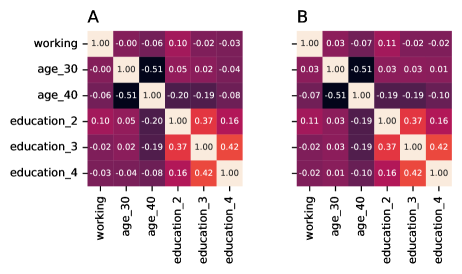
Figure 1: Pearson correlation matrix of the reader data, empirically computed from the data (A) and reproduced by the model (B).

IV Categorical factor analysis

As an application of multivariate categorical and ordinal variables, this section consider factor analysis for categorical and ordinal variables. The proposed factor analysis is achieved by setting the parameter $\Lambda$ for the Grassmann distribution by a block-diagonal matrix such that each block element of $\Lambda-I$ is a quasi-diagonal matrix with nonnegative principal minors, $\Psi^{-1}-I$ defined in Sec. II.2. This setting means that there is no correlation among categorical and ordinal variables given the latent variable. The positivity of probability distribution can be confirmed by direct calculations of principal minors of the matrix $\Lambda-I$, rather than diagonal dominance of parsimonious parametrization.

We denote observed continuous and binary dummy variables by $\mathbf{x}$ and $\mathbf{y}$ and denote continuous latent variables by $\mathbf{z}$. Each variable is a column vector and its dimensions are $p_{x}$, $q$, and $p_{z}$, respectively. Here, the states of the dummy vector $\mathbf{y}$ are limited to the state that are allowed for categorical and ordinal variables as described in Sec. II.1. We give the conditional distribution for the observed variables given the latent variable as a product of an uncorrelated normal distribution and uncorrelated Categorical and Ordinal distribution as follows:

$$p(\mathbf{x},\mathbf{y}|\mathbf{z})= \mathcal{N}\bigl{(}\mathbf{x}\mid\bm{\mu}_{x}+W(\mathbf{z}-\bm{\mu}_{z}),\Psi\bigr{)}\prod_{j=1}^{c}\mathrm{Cat}(\mathbf{y}_{C_{j}}\mid\bm{\beta}_{C_{j}})\;\prod_{k=1}^{o}\mathrm{Ord}(\mathbf{y}_{O_{k}}\mid\bm{\beta}_{O_{k}}),$$ (57)

$$\bm{\beta}= \mathbf{b}+G(\mathbf{z}-\bm{\mu}_{z}),\hskip 14.22636ptG\equiv\begin{bmatrix}\mathbf{g}_{1},\;\;\mathbf{g}_{2},\;\;\dots,\;\;\mathbf{g}_{q}\end{bmatrix}^{T},$$ (58)

where we define the categorical and ordinal distribution as follows:

$$\mathrm{Cat}(\mathbf{y}_{C_{j}}\mid\bm{\beta}_{C_{j}})=\frac{\exp(\mathbf{y}_{C_{j}}^{T}\bm{\beta}_{C_{j}})}{1+\sum_{l=1}^{q_{C_{j}}}\exp([\bm{\beta}_{C_{j}}]_{l})},\hskip 14.22636pt\mathrm{Ord}(\mathbf{y}_{O_{j}}\mid\bm{\beta}_{O_{j}})=\frac{\exp(\mathbf{y}_{O_{j}}^{T}\bm{\beta}_{O_{j}})}{1+\sum_{l=1}^{q_{O_{j}}}\prod_{m=1}^{l}\exp([\bm{\beta}_{O_{j}}]_{m})}.$$ (59)

The above conditional distribution is parameterized by $(\bm{\mu}_{x},\Psi,W)$ for continuous variables and $(\mathbf{b},G)$ for categorical and ordinal dummy variables. The $p_{x}$-dimensional column vector $\bm{\mu}_{x}$ parameterizes the mean of observed continuous variables, and the $p_{x}\times p_{x}$ diagonal matrix $\Psi$ is a covariance matrix of observational noise. The $p_{x}\times p_{z}$ matrix $W$ is a factor loading matrix for continuous variables Murphy (2012). The $q$-dimensional column vector $\mathbf{b}$ represents a bias term of the categorical and ordinal distributions, and the $q\times p_{z}$ matrix $G$ is a factor loading matrix for categorical and ordinal dummy variables. We shall call each row vector of factor loading matrix $G$ a factor loading vector $\mathbf{g}_{r}$.

The prior distribution of the latent variable is given by a mixture of normal distributions,

$$p(\mathbf{z})= \sum_{R_{1}\subseteq R}\pi_{R_{1}}(\Sigma_{z})\,\mathcal{N}(\mathbf{z}\mid\bm{\mu}_{z}+\Sigma_{z}G^{T}\bm{1}_{R_{1}},\Sigma_{z}),$$ (60)

$$\pi_{R_{1}}(\Sigma_{z})\equiv \frac{\exp\Bigl{(}\bm{1}_{R_{1}}^{T}\mathbf{b}+\frac{1}{2}\bm{1}_{R_{1}}^{T}G\Sigma_{z}G^{T}\bm{1}_{R_{1}}\Bigr{)}}{\sum_{R_{1}^{\prime}\subseteq R}\exp\Bigl{(}\bm{1}_{R_{1}^{\prime}}^{T}\mathbf{b}+\frac{1}{2}\bm{1}_{R_{1}^{\prime}}^{T}G\Sigma_{z}G^{T}\bm{1}_{R_{1}^{\prime}}\Bigr{)}},$$ (61)

where the summation $\sum_{R_{1}\subseteq R}$ runs over all states of the dummy variables allowed for the categorical and ordinal variables, not the states of all possible dummy variables, and $\bm{1}_{R_{1}}$ is a $q$-dimensional constant vector with each element taking the value $0$ or $1$,

$$[\bm{1}_{R_{1}}]_{s}\equiv\begin{cases}1,\hskip 14.22636pt\text{if}\;\;s\in R_{1},\\ 0,\hskip 14.22636pt\text{if}\;\;s\in R_{0},\end{cases}\;\;(s=1,2,\dots,q).$$ (62)

The parameters $(\bm{\mu}_{z},\Sigma_{z})$ are the mean and covariance of the prior distribution of the latent variable.

Then, the distribution for observed variables is given by

$$p(\mathbf{x},\mathbf{y})= \pi_{R_{1}}(\Sigma_{z})\,\mathcal{N}(\mathbf{x}\mid\bm{\mu}_{x}+W\Sigma_{z}G^{T}\mathbf{y},\Sigma_{x}),$$ (63)

$$\Sigma_{x}= \Psi+W\Sigma_{z}W^{T}.$$ (64)

When the observed variables consist exclusively of dummy variables, the observed distribution is nothing but the Ising model Ising (1925).

The posterior distribution of the latent variable given the observed variables is a normal distribution:

$$p(\mathbf{z}|\mathbf{x},\mathbf{y})= \mathcal{N}(\mathbf{z}\mid\mathbf{m},\Sigma_{z|x}),$$ (65)

$$\mathbf{m}= \bm{\mu}_{z}+\Sigma_{z|x}\bigl{\{}W^{T}\Psi^{-1}(\mathbf{x}-\bm{\mu}_{x})+G^{T}\mathbf{y}\bigr{\}},$$ (66)

$$\Sigma_{z|x}= \bigl{(}\Sigma_{z}^{-1}+W^{T}\Psi^{-1}W\bigr{)}^{-1}.$$ (67)

We call $\mathbf{m}$ in the above expression a factor score.

IV.1 Biplot analysis

In the biplot of factor analysis, we first plot the factor scores, Eq. (66), as a scatterplot. Without loss of generality, we set $\bm{\mu}_{z}=\bm{0}$ and $\Sigma_{z}=I$. Since categorical and ordinal variables are expressed by the combination of dummy variables, it is appropriate to express the factor loading vector, which is depicted by an arrow in the biplot, by a combination of factor loading vectors rather than by a single factor loading vector. We define the combined factor loading vectors for categorical and ordinal variables as follows:

$$\mathbf{g}_{l}^{(C_{j})}= -\frac{1}{q_{C_{j}}+1}\mathbf{g}_{C_{j}}+\mathbf{g}_{\mathrm{min}(C_{j})+l-1},\hskip 14.22636pt(l=1,2,\dots,q_{C_{j}}),$$ (68)

$$\mathbf{g}_{0}^{(C_{j})}= -\frac{1}{q_{C_{j}}+1}\mathbf{g}_{C_{j}},$$ (69)

$$\mathbf{g}_{l}^{(O_{j})}= -\frac{1}{2}\mathbf{g}_{O_{j}}+\sum_{m=1}^{l}\mathbf{g}_{\mathrm{min}(O_{j})+m-1},\hskip 14.22636pt(l=1,2,\dots,q_{O_{j}}),$$ (70)

$$\mathbf{g}_{0}^{(O_{j})}= -\frac{1}{2}\mathbf{g}_{O_{j}}.$$ (71)

New combined factor loading vectors, $\mathbf{g}_{0}^{(C_{j})}$ and $\mathbf{g}_{0}^{(O_{j})}$, correspond to the base category and the base level, where all dummy variables belonging to certain categorical or ordinal variable, take the value of zero, and satisfies

$$\mathbf{g}_{0}^{(C_{j})}=-\sum_{l=1}^{q_{C_{j}}}\mathbf{g}_{l}^{(C_{j})},\hskip 25.6073pt\mathbf{g}_{0}^{(O_{j})}=-\mathbf{g}_{q_{O_{j}}}^{(O_{j})}.$$ (72)

The inner product of the combined factor loading vectors and the factor scores represents the relative magnitude of the arguments of the categorical and ordinal distributions. That is, the large value of the inner product means that the corresponding categorical or ordinal feature is likely to occur than the mean value at that factor score.

We impose the norm constraints that all the combined factor loading vectors have the same norm, in order to avoid improper solutions, or Heywood cases, of maximum likelihood estimation in factor analysis, which has been devised in Ref. Arai (2022). Also, as in the previous paper Arai (2022), we fixed the rotational degrees of freedom of the latent space so that the matrix $GG^{T}$ is diagonalized. We defined the contribution ratio of the latent space, the principal component axes, by the eigenvalues of $GG^{T}$, and sorted the principal component axes in descending order of the contribution ratio.

We performed factor analysis on the reader data analyzed in the previous section. Model parameters were estimated by maximum likelihood estimation. The number of latent dimensions was selected by the Bayesian information criterion Schwarz (1978). The number of latent dimensions selected was two. Fig. 2 shows the biplot of factor analysis. The first and second principal component axes (PC1, PC2), the latent dimensions, are displayed, and the percentages in the axis labels represent the contribution ratio, When compressed into two dimensions, inequal intervals of the ordinal variable are visualized as angles of a protractor. We see that the first principal component axis can be interpreted as representing educated knowledge, and is related to the reading behavior of the women’s journal.

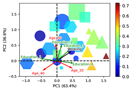
Figure 2: Biplot of factor analysis for reader data. The point characters in the scatterplot have been changed depending on the quarter value of the percentage of regular readers to a specific woman’s journal: the circles denote the data with a percentage smaller than the value of one-quarter, the hexagons are between one-quarter and two-quarter, the squares are between two-quarter and three quarter, and the triangles are larger than the value of three-quarter. Those markers are colored from blue to red according to small to large percentages. The areas of the point characters in the scatterplot are proportional to the number of data points corresponding to those point characters.

V Conclusion

We proposed a method to express correlations of multivariate categorical and ordinal variables in the framework of the Grassmann distribution in conjunction with dummy encoding of categorical and ordinal variables. The proposed distribution allows undesirable co-occurrence probabilities of categorical and ordinal dummy variables to be exactly zero. Furthermore, unlike the method of quantification, the proposed method works retaining the nature of the scale of categorical and ordinal variables, i.e., nominal and ordinal scales. As an application of the proposed distribution, we develop a factor analysis for categorical and ordinal variables. Our biplot of factor analysis can be used as an alternative to correspondence analysis Hirschfeld (1935).

A series of studies from the previous research Arai (2021, 2022) to this paper has produced probability distributions that describe linear correlations for the major three of the four statistical data types: ratio scale, nominal scale, and ordinal scale Stevens (1946). These distributions allow us to construct probabilistic generative models for a mixture of continuous and qualitative variables. We expect that the results of these studies open new directions for the quantitative analysis of qualitative data and provide the basis for building more advanced statistical learning methods.

Appendix A Inverted Grassmann distribution

In this appendix, we summarize the probability distribution in which the effect of dummy variables is inverted from that of the previous studies Arai (2021, 2022), to avoid possible confusion.

We denote $p$-dimensional continuous variables and $q$-dimensional dummy variables by column vectors $\mathbf{x}$ and $\mathbf{y}$, respectively. The dummy vector $\mathbf{y}$ is a bit vector with each element taking the value $0$ or $1$. Model parameters of our distribution consist of mean and covariance parameters of a multivariate normal distribution $(\bm{\mu},\Sigma)$, a $q\times q$ matrix of the Grassmann distribution $\Lambda$ (Arai, 2021), and a $q\times p$ matrix $G$ representing interaction between continuous and binary variables. The matrix $\Lambda-I$ must be a $P_{0}$-matrix (Tsatsomeros, 2002), where $I$ is an identity matrix. Each element of the matrix $G$, $[G]_{sj},\;(s=1,2,\dots,q,\;\text{and}\;\;j=1,2,\dots,p)$, is also represented by a $p$-dimensional column vector $\mathbf{g}_{s}$ as

$$G\equiv\begin{bmatrix}\mathbf{g}_{1},\;\;\mathbf{g}_{2},\;\;\dots,\;\;\mathbf{g}_{q}\end{bmatrix}^{T},\hskip 14.22636pt[G]_{sj}=[\mathbf{g}_{s}^{T}]_{j},$$ (73)

where $T$ stands for matrix transposition. We denote the set of whole indices of continuous and binary variables as $I\equiv\{1,2,\dots,p\}$ and $R\equiv\{1,2,\dots,q\}$, respectively. An index label for binary variables is divided into two parts with subscripts $1$ and $0$, for variables that take the value $1$ and $0$, respectively. For example, an index label for binary variables $R$ is divided into a subset $R_{1}\subseteq R$ and its set difference $R_{0}=R\setminus R_{1}$. We denote a $q$-dimensional constant vector $\bm{1}_{R_{1}}$ with each element taking the value $0$ or $1$,

$$[\bm{1}_{R_{1}}]_{s}\equiv\begin{cases}1,\hskip 14.22636pt\text{if}\;\;s\in R_{1}\\ 0,\hskip 14.22636pt\text{if}\;\;s\in R_{0}\end{cases},\;\;(s=1,2,\dots,q).$$ (74)

Then, the proposed jont distribution is expressed as

$$p(\mathbf{x},\mathbf{y}=\bm{1}_{R_{1}})= \pi_{R_{1}}(\Sigma)\,\mathcal{N}(\mathbf{x}\mid\bm{\mu}+\Sigma G^{T}\bm{1}_{R_{1}},\Sigma),$$

$$\equiv \pi_{R_{1}}(\Sigma)\frac{1}{(2\pi)^{p/2}\det\Sigma^{1/2}}\,\exp\left\{-\frac{1}{2}(\mathbf{x}-\bm{\mu}-\Sigma G^{T}\bm{1}_{R_{1}})^{T}\Sigma^{-1}(\mathbf{x}-\bm{\mu}-\Sigma G^{T}\bm{1}_{R_{1}})\right\},$$ (75)

$$\pi_{R_{1}}(\Sigma)\equiv \frac{\det(\Lambda_{R_{1}R_{1}}-I)\exp\Bigl{(}\frac{1}{2}\bm{1}_{R_{1}}^{T}G\Sigma G^{T}\bm{1}_{R_{1}}\Bigr{)}}{\sum_{R_{1}^{\prime}\subseteq R}\det(\Lambda_{R_{1}^{\prime}R_{1}^{\prime}}-I)\exp\Bigl{(}\frac{1}{2}\bm{1}_{R_{1}^{\prime}}^{T}G\Sigma G^{T}\bm{1}_{R_{1}^{\prime}}\Bigr{)}},$$ (76)

where $\Lambda_{R_{1}R_{1}}$ is a submatrix of $\Lambda$, and summation $\sum_{R_{1}^{\prime}\subseteq R}$ runs over all possible states of binary variables. The partition function, the normalization constant, of this distribution is not given analytically, and thus, one has to sum over all possible states of the binary variables to calculate the partition function. As we will see below, the coefficient $\pi_{R_{1}}(\Sigma)$ corresponds to mixing weight of a mixture of Gaussian distributions with equal covariance. That is, the above joint distribution corresponds to one normal distribution out of $2^{q}$ mixture of normal distributions.

To express the marginal and conditional distributions, we first define the notation of index. We denote the index label of a subset of whole indices as $J\subseteq I$. Then, the subvector comprising the subset of indices $J$ is represented as $\mathbf{x}_{J}$. We divide the sets of whole indices of continuous and binary variables into three subset parts; $I=(J,L,K)$ and $R=(S,U,T)$, where the index labels $L$ and $U$ are introduced to handle missing values. The number of elements in these sets of indices is represented by $p_{J}$, $p_{L}$, $p_{K}$ and $q_{S}$, $q_{U}$, $q_{T}$, these of course satisfy $p_{J}+p_{L}+p_{K}=p$ and $q_{S}+q_{U}+q_{T}=q$. Then, the vectors $\mathbf{x}$ and $\mathbf{y}$ can be partitioned into subvectors as $\mathbf{x}=\mathbf{x}_{I}=(\mathbf{x}_{J},\mathbf{x}_{L},\mathbf{x}_{K})$ and $\mathbf{y}=\mathbf{y}_{R}=(\mathbf{y}_{S},\mathbf{y}_{U},\mathbf{y}_{T})$, respectively. Again, an index label for binary variables is further divided into two parts with subscripts $1$ and $0$, for variables that take the value $1$ and $0$, respectively. For example, an index label for binary variables $S\subseteq R$ is divided into a subset $S_{1}\subseteq S$ and its set difference $S_{0}=S\setminus S_{1}$, where the subvectors $\mathbf{y}_{S_{1}}$ and $\mathbf{y}_{S_{0}}$ take the values as $\mathbf{y}_{S_{1}}=\bm{1}$ and $\mathbf{y}_{S_{0}}=\bm{0}$, respectively. The union of the index label $J$ and $K$ is denoted as $J+K\equiv J\cup K$. Using the index notation described above, the marginal distribution is expressed as

$$p(\mathbf{x}_{K}=\mathbf{x}_{I\setminus(J+L)},\mathbf{y}_{T}=\mathbf{y}_{R\setminus(S+U)})= \sum_{S_{1}+U_{1}\subseteq R\setminus T}\pi_{R_{1}}(\Sigma)\,\mathcal{N}(\mathbf{x}_{K}\mid\bm{\mu}_{K}+\Sigma_{KI}G^{T}\bm{1}_{R_{1}},\Sigma_{KK}).$$ (77)

In particular, when all binary variables are marginalized, the marginal distribution is precisely a $2^{q}$ mixture of Gaussian distributions with equal covariance, where mixing weights are given by $\pi_{R_{1}}(\Sigma)$ and the mean of the normal distributions is shifted by $\Sigma G^{T}\bm{1}_{R_{1}}$. On the other hand, when all continuous variables are marginalized, the marginal distribution is no longer in the same form as the Grassmann distribution.

The conditional distribution with missing values for $\mathbf{x}_{L}$ and $\mathbf{y}_{U}$ is given by

$$p(\mathbf{x}_{J},\mathbf{y}_{S}|\mathbf{x}_{K},\mathbf{y}_{T})= \frac{\sum_{U_{1}\subseteq R\setminus(S+T)}\pi_{R_{1}}\bigl{(}\Sigma_{(J+L)|K}\bigr{)}\exp\Bigl{\{}\bm{1}_{R_{1}}^{T}G\Sigma_{IK}\Sigma_{KK}^{-1}(\mathbf{x}_{K}-\bm{\mu}_{K})\Bigr{\}}}{\sum_{S_{1}^{\prime}+U_{1}^{\prime}\subseteq R\setminus T}\pi_{R_{1}^{\prime}}\bigl{(}\Sigma_{(J+L)|K}\bigr{)}\exp\Bigl{\{}\bm{1}_{R_{1}^{\prime}}^{T}G\Sigma_{IK}\Sigma_{KK}^{-1}(\mathbf{x}_{K}-\bm{\mu}_{K})\Bigr{\}}}$$

$$\mathcal{N}\bigl{(}\mathbf{x}_{J}\mid\bm{\mu}_{J}+\Sigma_{JK}\Sigma_{KK}^{-1}(\mathbf{x}_{K}-\bm{\mu}_{K})+(\Sigma_{J(J+L)}-\Sigma_{JK}\Sigma_{KK}^{-1}\Sigma_{K(J+L)})G_{(J+L)R}^{T}\bm{1}_{R_{1}},\Sigma_{J|K}\bigr{)},$$ (78)

where $\Sigma_{KK}^{-1}$ denotes the inverse matrix of the submatrix $\Sigma_{KK}$, the matrix $\Sigma_{J|K}\equiv\Sigma_{JJ}-\Sigma_{JK}\Sigma_{KK}^{-1}\Sigma_{KJ}$ is the Schur complement, and the mixing weight is defined as previously mentioned,

$$\pi_{R_{1}}\bigl{(}\Sigma_{(J+L)|K}\bigr{)}\equiv\frac{\det(\Lambda_{R_{1}R_{1}}-I)\exp\Bigl{\{}\frac{1}{2}\bm{1}_{R_{1}}^{T}G_{R(J+L)}\Sigma_{(J+L)|K}G_{(J+L)R}^{T}\bm{1}_{R_{1}}\Bigr{\}}}{\sum_{R_{1}^{\prime}\subseteq R}\det(\Lambda_{R_{1}^{\prime}R_{1}^{\prime}}-I)\exp\Bigl{\{}\frac{1}{2}\bm{1}_{R_{1}^{\prime}}^{T}G_{R(J+L)}\Sigma_{(J+L)|K}G_{(J+L)R}^{T}\bm{1}_{R_{1}^{\prime}}\Bigr{\}}}.$$ (79)

When there are no missing values, the conditional distribution is expressed more concisely:

$$p(\mathbf{x}_{J},\mathbf{y}_{S}|\mathbf{x}_{K}=\mathbf{x}_{I\setminus J},\mathbf{y}_{T}=\mathbf{y}_{R\setminus S})= \frac{\pi_{R_{1}}(\Sigma_{J|K})\exp\Bigl{\{}\bm{1}_{S_{1}}^{T}G\Sigma_{IK}\Sigma_{KK}^{-1}(\mathbf{x}_{K}-\bm{\mu}_{K})\Bigr{\}}}{\sum_{S_{1}^{\prime}\subseteq R\setminus T}\pi_{R_{1}^{\prime}}(\Sigma_{J|K})\exp\Bigl{\{}\bm{1}_{S_{1}^{\prime}}^{T}G\Sigma_{IK}\Sigma_{KK}^{-1}(\mathbf{x}_{K}-\bm{\mu}_{K})\Bigr{\}}}$$

$$\mathcal{N}\bigl{(}\mathbf{x}_{J}\mid\bm{\mu}_{J}+\Sigma_{JK}\Sigma_{KK}^{-1}(\mathbf{x}_{K}-\bm{\mu}_{K})+\Sigma_{J|K}G_{JR}^{T}\bm{1}_{R_{1}},\Sigma_{J|K}\bigr{)}.$$ (80)

In particular, when observed variables consist exclusively of binary variables, the conditional distribution is expressed as a normal distribution,

$$p(\mathbf{x}_{J}|\mathbf{x}_{K}=\mathbf{x}_{I\setminus J},\mathbf{y}_{R})= \mathcal{N}\left(\mathbf{x}_{J}\mid\bm{\mu}_{J}+\Sigma_{JK}\Sigma_{KK}^{-1}(\mathbf{x}_{K}-\bm{\mu}_{K})+\Sigma_{J|K}G^{T}\bm{1}_{R_{1}},\Sigma_{J|K}\right),$$ (81)

there, the mean of the distribution is shifted depending on the value of the binary variables conditioned. On the other hand, when observed variables consist exclusively of continuous variables, the conditional distribution is expressed as a Grassmann distribution:

$$p(\mathbf{y}_{S}|\mathbf{x}_{I},\mathbf{y}_{T}=\mathbf{y}_{R\setminus S})= \mathcal{G}^{(1)}\bigl{(}\mathbf{y}_{S}\mid I+(\Lambda-I)_{S|T_{1}}\,\mathrm{Exp}\bigl{\{}G_{SI}(\mathbf{x}_{I}-\bm{\mu}_{I})\bigr{\}}\bigr{)},$$

$$\equiv \frac{\det\bigl{[}(\Lambda-I)_{S_{1}|T_{1}}\,\mathrm{Exp}\bigl{\{}G_{S_{1}I}(\mathbf{x}_{I}-\bm{\mu}_{I})\bigr{\}}\bigr{]}}{\det\bigl{[}I+(\Lambda-I)_{S|T_{1}}\,\mathrm{Exp}\bigl{\{}G_{SI}(\mathbf{x}_{I}-\bm{\mu}_{I})\bigr{\}}\bigr{]}},$$ (82)

$$(\Lambda-I)_{S|T_{1}}\equiv \Lambda_{SS}-I-\Lambda_{ST_{1}}(\Lambda_{T_{1}T_{1}}-I)^{-1}\Lambda_{T_{1}S},$$ (83)

where

$$\mathrm{Exp}\bigl{\{}G_{SI}(\mathbf{x}_{I}-\bm{\mu}_{I})\bigr{\}}\equiv E^{G_{SI}(\mathbf{x}_{I}-\bm{\mu}_{I})}\equiv\mathrm{diag}\bigl{[}\exp\bigl{\{}\mathbf{g}_{s}^{T}(\mathbf{x}_{I}-\bm{\mu}_{I})\bigr{\}}\bigr{]},\hskip 14.22636pts\in S$$ (84)

is a diagonal matrix with nonnegative diagonal elements.

References