Improving Few-Shot Inductive Learning on Temporal Knowledge Graphs using Confidence-Augmented Reinforcement Learning

Abstract

Temporal knowledge graph completion (TKGC) aims to predict the missing links among the entities in a temporal knwoledge graph (TKG). Most previous TKGC methods only consider predicting the missing links among the entities seen in the training set, while they are unable to achieve great performance in link prediction concerning newly-emerged unseen entities. Recently, a new task, i.e., TKG few-shot out-of-graph (OOG) link prediction, is proposed, where TKGC models are required to achieve great link prediction performance concerning newly-emerged entities that only have few-shot observed examples. In this work, we propose a TKGC method FITCARL that combines few-shot learning with reinforcement learning to solve this task. In FITCARL, an agent traverses through the whole TKG to search for the prediction answer. A policy network is designed to guide the search process based on the traversed path. To better address the data scarcity problem in the few-shot setting, we introduce a module that computes the confidence of each candidate action and integrate it into the policy for action selection. We also exploit the entity concept information with a novel concept regularizer to boost model performance. Experimental results show that FITCARL achieves stat-of-the-art performance on TKG few-shot OOG link prediction. Code and supplementary appendices are provided.

1 Introduction

Knowledge graphs (KGs) store knowledge by representing facts in the form of triples, i.e, $(s,r,o)$, where $s$ and $o$ are the subject and object entities, and $r$ denotes the relation between them. To further specify the time validity of the facts, temporal knowledge graphs (TKGs) are introduced by using a quadruple $(s,r,o,t)$ to represent each fact, where $t$ is the valid time of this fact. In this way, TKGs are able to capture the ever-evolving knowledge over time. It has already been extensively explored to use KGs and TKGs to assist downstream tasks, e.g., question answering [48, 30, 12] and natural language generation [2, 22].

Since TKGs are known to be incomplete [21], a large number of researches focus on proposing methods to automatically complete TKGs, i.e., temporal knowledge graph completion (TKGC). In traditional TKGC, models are given a training set consisting of a TKG containing a finite set of entities during training, and they are required to predict the missing links among the entities seen in the training set. Most previous TKGC methods, e.g., [34, 21, 19, 11], achieve great success on traditional TKGC, however, they still have drawbacks. (1) Due to the ever-evolving nature of world knowledge, new unseen entities always emerge in a TKG and traditional TKGC methods fail to handle them. (2) Besides, in real-world scenarios, newly-emerged entities are usually coupled with only a few associated edges [13]. Traditional TKGC methods require a large number of entity-related data examples to learn expressive entity representations, making them hard to optimally represent newly-emerged entities. To this end, recently, Ding et al. [13] propose the TKG few-shot out-of-graph (OOG) link prediction (LP) task based on traditional TKGC, aiming to draw attention to studying how to achieve better LP results regarding newly-emerged TKG entities.

In this work, we propose a TKGC method to improve few-shot inductive learning over newly-emerged entities on TKGs using confidence-augmented rein-forcement learning (FITCARL). FITCARL is developed to solve TKG few-shot OOG LP [13]. It is a meta-learning based method trained with episodic training [39]. For each unseen entity, FITCARL first employs a time-aware Transformer [38] to adaptively learn its expressive representation. Then it starts from the unseen entity and sequentially takes actions by transferring to other entities according to the observed edges associated with the current entity, following a policy parameterized by a learnable policy network. FITCARL traverses the TKG for a fixed number of steps and stops at the entity that is expected to be the LP answer. To better address the data scarcity problem in the few-shot setting, we introduce a confidence learner that computes the confidence of each candidate action and integrate it into the policy for action selection. Following [13], we also take advantage of the concept information presented in the temporal knowledge bases (TKBs) and design a novel concept regularizer. We summarize our contributions as follows: (1) This is the first work using reinforcement learning-based method to reason over newly-emerged few-shot entities in TKGs and solve the TKG few-shot OOG LP task. (2) We propose a time-aware Transformer using a time-aware positional encoding method to better utilize few-shot information in learning representations of new-emerged entities. (3) We design a novel confidence learner to alleviate the negative impact of the data scarcity problem brought by the few-shot setting. (4) We propose a parameter-free concept regularizer to utilize the concept information provided by the TKBs and it demonstrates strong effectiveness. (5) FITCARL achieves state-of-the-art performance on all datasets of TKG few-shot OOG LP and provides explainability.

2 Related Work

2.1 Knowledge Graph & Temporal Knowledge Graph Completion

Knowledge graph completion (KGC) methods can be summarized into two types. First type of methods focus on designing KG score functions that directly compute the plausibility scores of KG triples [5, 24, 1, 27, 46, 35, 4]. Second type of KGC methods are neural-based models [31, 37]. Neural-based models are built by coupling KG score functions with neural structures, e.g., graph neural network (GNN). It is shown that neural structures make great contributions to enhancing the performance of KGC methods. TKGC methods are developed by incorporating temporal reasoning techniques. A line of work aims to design time-aware KG score functions that are able to process time information [21, 45, 29, 25, 7, 47]. Another line of work employs neural structures to encode temporal information, where some work uses recurrent neural structures, e.g., Transformer [38], to model the temporal dependencies in TKGs [42], and other work designs time-aware GNNs to achieve temporal reasoning by computing time-aware entity representations through aggregation [19, 11]. Reinforcement learning (RL) has already been used to reason TKGs, e.g., [33, 23]. TITer [33] and CluSTeR [23] achieves temporal path modeling with RL. However, they are traditional TKG reasoning models and are not designed to deal with few-shot unseen entities.

2.2 Inductive Learning on KGs & TKGs

In recent years, inductive learning on KGs and TKGs has gained increasing interest. A series of work [43, 8, 32, 26, 10] focuses on learning strong inductive representations of few-shot unseen relations using meta-learning-based approaches. These methods achieve great effectiveness, however, they are unable to deal with newly-emerged entities. Some work tries to deal with unseen entities by inductively transferring knowledge from seen to unseen entities with an auxiliary set provided during inference [15, 40, 17]. Their performance highly depends on the size of the auxiliary set. [13] shows that with a tiny auxiliary set, these methods cannot achieve ideal performance. Besides, these methods are developed for static KGs, thus without temporal reasoning ability. On top of them, Baek et al. [3] propose a more realistic task, i.e., KG few-shot OOG LP, aiming to draw attention to better studying few-shot OOG entities. They propose a model GEN that contains two GNNs and train it with a meta-learning framework to adapt to the few-shot setting. Same as [15, 40, 17], GEN does not have a temporal reasoning module, and therefore, it cannot reason TKGs. Ding et al. [13] propose the TKG few-shot OOG LP task that generalizes [3] to the context of TKGs. They develop a meta-learning-based model FILT that achieves temporal reasoning with a time difference-based graph encoder and mines concept-aware information from the entity concepts specified in TKBs. Recently, another work [41] proposes a task called few-shot TKG reasoning, aiming to ask TKG models to predict future facts for newly-emerged few-shot entities. In few-shot TKG reasoning, for each newly-emerged entity, TKG models are asked to predict the unobserved associated links happening after the observed few-shot examples. Such restriction is not imposed in TKG few-shot OOG LP, meaning that TKG models should predict the unobserved links happening at any time along the time axis. In our work, we only consider the task setting of TKG few-shot OOG LP and do not consider the setting of [41].

3 Task Formulation and Preliminaries

3.1 TKG Few-Shot Out-of-Graph Link Prediction

Definition 1 (TKG Few-Shot OOG LP). Assume we have a background TKG $\mathcal{G}_{\text{back}}=\{(s,r,o,t)|s,o\in\mathcal{E}_{\text{back}},r\in\mathcal{R},t\in\mathcal{T}\}\subseteq\mathcal{E}_{\text{back}}\times\mathcal{R}\times\mathcal{E}_{\text{back}}\times\mathcal{T}$, where $\mathcal{E}_{\text{back}}$, $\mathcal{R}$, $\mathcal{T}$ denote a finite set of seen entities, relations and timestamps, respectively. An unseen entity $e^{\prime}$ is an entity $e^{\prime}\in\mathcal{E^{\prime}}$ and $\mathcal{E}^{\prime}\cap\mathcal{E}_{\text{back}}=\emptyset$. For each $e^{\prime}\in\mathcal{E}^{\prime}$, given $K$ observed $e^{\prime}$ associated TKG facts $(e^{\prime},r,\tilde{e},t)$ (or $(\tilde{e},r,e^{\prime},t)$), where $\tilde{e}\in(\mathcal{E}_{\text{back}}\cup\mathcal{E}^{\prime})$, $r\in\mathcal{R}$, $t\in\mathcal{T}$, TKG few-shot OOG LP asks models to predict the missing entities of LP queries $(e^{\prime},r_{q},?,t_{q})$ (or $(?,r_{q},e^{\prime},t_{q})$) derived from unobserved TKG facts containing $e^{\prime}$ ($r_{q}\in\mathcal{R}$, $t_{q}\in\mathcal{T}$). $K$ is a small number denoting shot size, e.g., 1 or 3.

Ding et al. [13] formulate TKG few-shot OOG LP into a meta-learning problem and uses episodic training [39] to train its model. For a TKG $\mathcal{G}\subseteq\mathcal{E}\times\mathcal{R}\times\mathcal{E}\times\mathcal{T}$, they split its entities into background (seen) entities $\mathcal{E}_{\text{back}}$ and unseen entities $\mathcal{E}^{\prime}$, where $\mathcal{E}^{\prime}\cap\mathcal{E}_{\text{back}}=\emptyset$ and $\mathcal{E}=(\mathcal{E}_{\text{back}}\cup\mathcal{E}^{\prime})$. A background TKG $\mathcal{G}_{\text{back}}\subseteq\mathcal{E}_{\text{back}}\times\mathcal{R}\times\mathcal{E}_{\text{back}}\times\mathcal{T}$ is constructed by including all the TKG facts that do not contain unseen entities. Then, unseen entities $\mathcal{E}^{\prime}$ are further split into three non-overlapped groups $\mathcal{E}^{\prime}_{\text{meta-train}}$, $\mathcal{E}^{\prime}_{\text{meta-valid}}$ and $\mathcal{E}^{\prime}_{\text{meta-test}}$. The union of all the facts associated to each group’s entities forms the corresponding meta-learning set, e.g., the meta-training set $\mathbb{T}_{\text{meta-train}}$ is formulated as $\{(e^{\prime},r,\tilde{e},t)|\tilde{e}\in\mathcal{E},r\in\mathcal{R},e^{\prime}\in\mathcal{E}^{\prime}_{\text{meta-train}},t\in\mathcal{T}\}\cup\{(\tilde{e},r,e^{\prime},t)|\tilde{e}\in\mathcal{E},r\in\mathcal{R},e^{\prime}\in\mathcal{E}^{\prime}_{\text{meta-train}},t\in\mathcal{T}\}$. Ding et al. ensure that there exists no link between every two of the meta-learning sets. During meta-training, models are trained over a number of episodes, where a training task $T$ is sampled in each episode. For each task $T$, $N$ unseen entities $\mathcal{E}_{T}$ are sampled from $\mathcal{E}^{\prime}_{\text{meta-train}}$. For each $e^{\prime}\in\mathcal{E}_{T}$, $K$ associated facts are sampled to form a support set $Sup_{e^{\prime}}=\{(e^{\prime},r_{i},\tilde{e}_{i},t_{i})\ \text{or}\ (\tilde{e}_{i},r_{i},e^{\prime},t_{i})|\tilde{e}_{i}\in(\mathcal{E}_{\text{back}}\cup\mathcal{E}^{\prime}),r_{i}\in\mathcal{R},t_{i}\in\mathcal{T}\}^{K}_{i=1}$, and the rest of its associated facts are taken as its query set $Que_{e^{\prime}}=\{(e^{\prime},r_{i},\tilde{e}_{i},t_{i})\ \text{or}\ (\tilde{e}_{i},r_{i},e^{\prime},t_{i})|\tilde{e}_{i}\in(\mathcal{E}_{\text{back}}\cup\mathcal{E}^{\prime}),r_{i}\in\mathcal{R},t_{i}\in\mathcal{T}\}^{M_{e^{\prime}}}_{i=K+1}$, where $M_{e^{\prime}}$ denotes the number of $e^{\prime}$’s associated facts. Models are asked to simultaneously perform LP over $Que_{e^{\prime}}$ for each $e^{\prime}\in\mathcal{E}_{T}$, given their $Sup_{e^{\prime}}$ and $\mathcal{G}_{\text{back}}$. After meta-training, models are validated with a meta-validation set $\mathbb{T}_{\text{meta-valid}}$ and tested with a meta-test set $\mathbb{T}_{\text{meta-test}}$. In our work, we also train FITCARL in the same way as [13] with episodic training on the same meta-learning problem.

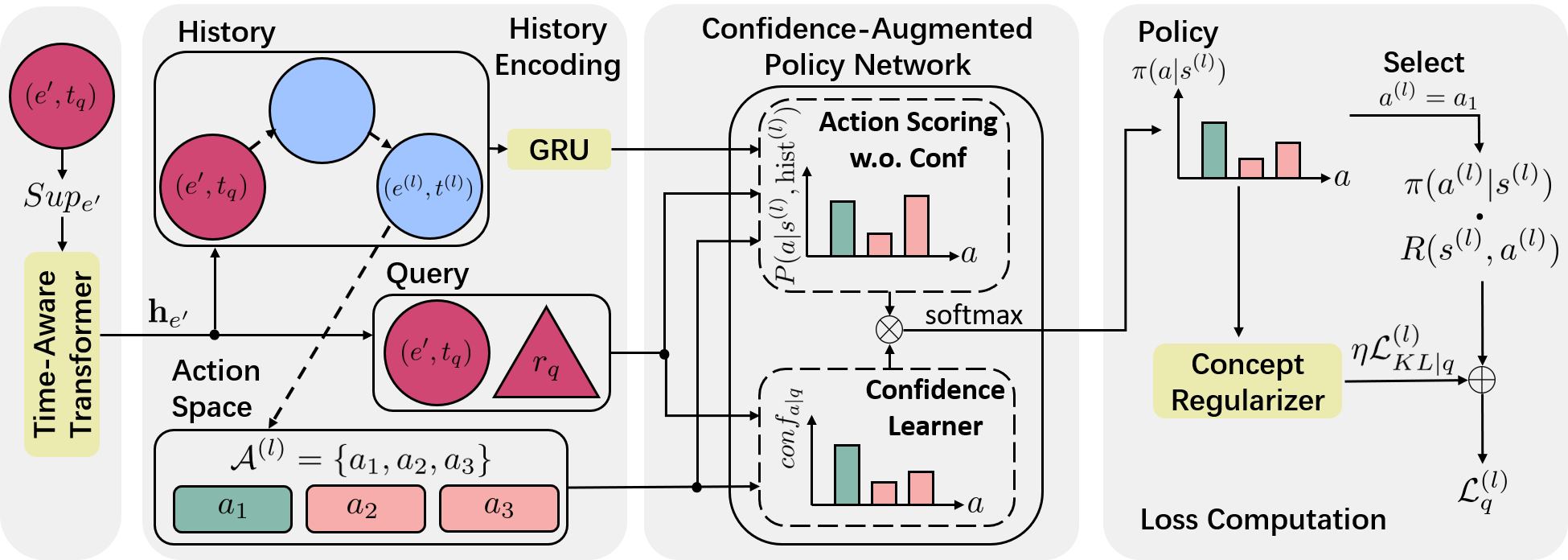
Figure 1: Overview of FITCARL. To do prediction over the LP query $q=(e^{\prime},r_{q},?,t_{q})$, FITCARL first learns $\mathbf{h}_{e^{\prime}}$ from a time-aware Transformer. It is then used in history encoding (with GRU) and policy network. To search for the answer, FITCARL starts from node $(e^{\prime},t_{q})$. It goes to $(e^{(l)},t^{(l)})$, state $s^{(l)}$, at step $l$. It computes a policy using a confidence-augmented policy network. Assume FITCARL selects action $a_{1}$ in current action space $\mathcal{A}^{(l)}$ as the current action $a^{(l)}$. We compute a loss $\mathcal{L}_{q}^{(l)}$ at step $l$, considering $a_{1}$’s probability in policy and reward $R(s^{(l)},a^{(l)})$, as well as an extra regularization loss $\eta\mathcal{L}_{KL|q}^{(l)}$ computed by a concept regularizer. Please refer to Section 4.1, 4.2 and 4.3 for details.

3.2 Concepts for Temporal Knowledge Graph Entities

[13] extracts the concepts of TKG entities by exploring the associated TKBs. Entity concepts describe the characteristics of entities. For example, in the Integrated Crisis Early Warning System (ICEWS) database [6], the entity Air Force (Canada) is described with the following concepts: Air Force, Military and Government. Ding et al. propose three ICEWS-based datasets for TKG few-shot OOG LP and manage to couple every entity with its unique concepts. We use $\mathcal{C}$ to denote all the concepts existing in a TKG and $\mathcal{C}_{e}$ to denote $e$’s concepts.

4 The Proposed FITCARL Model

Given the support set $Sup_{e^{\prime}}=\{(e^{\prime},r_{i},\tilde{e}_{i},t_{i})\ \text{or}\ (\tilde{e}_{i},r_{i},e^{\prime},t_{i})\}^{K}_{i=1}$ of $e^{\prime}\in\mathcal{E}^{\prime}$, assume we want to predict the missing entity from the LP query $q=(e^{\prime},r_{q},?,t_{q})$ derived from a query quadruple $(e^{\prime},r_{q},\tilde{e}_{q},t_{q})\in Que_{e^{\prime}}$. To achieve this, FITCARL first learns a representation $\mathbf{h}_{e^{\prime}}\in\mathbb{R}^{d}$ ($d$ is dimension size) for $e^{\prime}$ (Section 4.1). Then it employs an RL agent that starts from the node $(e^{\prime},t_{q})$ and sequentially takes actions by traversing to other nodes (in the form of (entity, timestamp)) following a policy (Section 4.2 and 4.3). After $L$ traverse steps, the agent is expected to stop at a target node containing $\tilde{e}_{q}$. Fig. 1 shows an overview of FITCARL during training, showing how it computes loss $\mathcal{L}_{q}^{(l)}$ at step $l$.

4.1 Learning Unseen Entities with Time-Aware Transformer

We follow FILT [13] and use the entity and relation representations pre-trained with ComplEx [35] for model initialization. Note that pre-training only considers all the background TKG facts, i.e., $\mathcal{G}_{\text{back}}$.

To learn $\mathbf{h}_{e^{\prime}}$, we start from learning $K$ separate meta-representations. Given $Sup_{e^{\prime}}$, we transform every support quadruple whose form is $(e^{\prime},r_{i},\tilde{e}_{i},t_{i})$ to $(\tilde{e}_{i},r_{i}^{-1},e^{\prime},t_{i})$, where $r_{i}^{-1}$ denotes the inverse relation of $r_{i}$. Then we create a temporal neighborhood $\mathcal{N}_{e^{\prime}}=\{(\tilde{e}_{i},r_{i},t_{i})|(\tilde{e}_{i},r_{i},e^{\prime},t_{i})\in Sup_{e^{\prime}}\ \text{or}\ (e^{\prime},r_{i}^{-1},\tilde{e}_{i},t_{i})\in Sup_{e^{\prime}}\}$ for $e^{\prime}$ based on $Sup_{e^{\prime}}$, where $|\mathcal{N}_{e^{\prime}}|=K$. We compute a meta-representation $\mathbf{h}_{e^{\prime}}^{i}$ from each temporal neighbor $(\tilde{e}_{i},r_{i},t_{i})$ as $\mathbf{h}_{e^{\prime}}^{i}=f(\mathbf{h}_{\tilde{e}_{i}}\|\mathbf{h}_{r_{i}})$, where $\mathbf{h}_{r_{i}}\in\mathbb{R}^{d}$ is the representation of the relation $r_{i}$ and $\|$ is the concatenation operation.

We collect $\{\mathbf{h}_{e^{\prime}}^{i}\}_{i=1}^{K}$ and use a time-aware Transformer to compute a contextualized representation $\mathbf{h}_{e^{\prime}}$. We treat each temporal neighbor $(\tilde{e}_{i},r_{i},t_{i})\in\mathcal{N}_{e^{\prime}}$ as a token and the corresponding meta-representation $\mathbf{h}_{e^{\prime}}^{i}$ as its token representation. We concatenate the classification ([CLS]) token with the temporal neighbors in $\mathcal{N}_{e^{\prime}}$ as a sequence and input it into a Transformer, where the sequence length is $K+1$. The order of temporal neighbors is decided by the sampling order of support quadruples.

To better utilize temporal information from temporal neighbors, we propose a time-aware positional encoding method. For any two tokens $u,v$ in the input sequence, we compute the time difference $t_{u}-t_{v}$ between their associated timestamps, and then map it into a time-difference representation $\mathbf{h}_{t_{u}-t_{v}}\in\mathbb{R}^{d}$,

$$\mathbf{h}_{t_{u}-t_{v}}=\sqrt{\frac{1}{d}}[cos(\omega_{1}(t_{u}-t_{v})+\phi_{1}),...,cos(\omega_{d}(t_{u}-t_{v})+\phi_{d}))].$$ (1)

$\omega_{1}$ to $\omega_{d}$ and $\phi_{1}$ to $\phi_{d}$ are trainable parameters. The timestamp for each temporal neighbor is $t_{i}$ and we set the timestamp of the [CLS] token to the query timestamp $t_{q}$ since we would like to use the learned $\mathbf{h}_{e^{\prime}}$ to predict the LP query happening at $t_{q}$. The attention $\text{att}_{u,v}$ of any token $v$ to token $u$ in an attention layer of our time-aware Transformer is written as

$$\text{att}_{u,v}=\frac{\text{exp}(\alpha_{u,v})}{\sum_{k=1}^{K+1}\text{exp}(\alpha_{u,k})},$$ (2)

$$\alpha_{u,v}=\frac{1}{\sqrt{d}}(\mathbf{W}_{TrQ}\mathbf{h}_{u})^{\top}(\mathbf{W}_{TrK}\mathbf{h}_{v})+{\mathbf{w}_{Pos}}^{\top}\mathbf{h}_{t_{u}-t_{v}}.$$

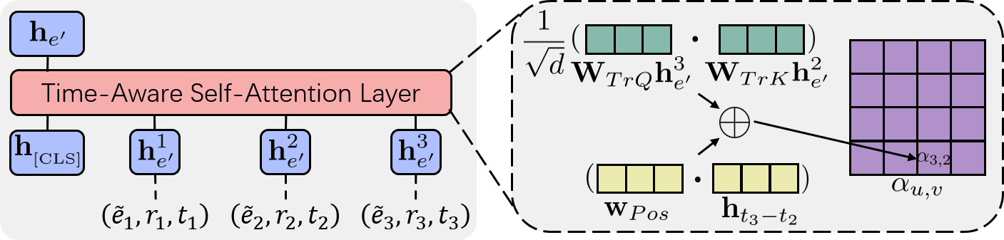
Figure 2: Time-aware Transformer with one attention layer for learning unseen entity representation in the 3-shot case.

$\mathbf{h}_{u},\mathbf{h}_{v}\in\mathbb{R}^{d}$ are the input representations of token $u,v$ into this attention layer. $\mathbf{W}_{TrQ},\mathbf{W}_{TrK}\in\mathbb{R}^{d\times d}$ are the weight matrices following original definition in [38]. $\mathbf{w}_{Pos}\in\mathbb{R}^{d}$ is a parameter that maps $\mathbf{h}_{t_{u}-t_{v}}$ to a scalar representing time-aware relative position from token $v$ to $u$. We use several attention layers and also employ multi-head attention to increase model expressiveness. The output representation of the [CLS] token from the last attention layer is taken as $\mathbf{h}_{e^{\prime}}$. Fig. 2 illustrates how the time-aware Transformer learns $\mathbf{h}_{e^{\prime}}$ in the 3-shot case.

4.2 Reinforcement Learning Framework

We formulate the RL process as a Markov Decision Process and we introduce its elements as follows. (1) States: Let $\mathcal{S}$ be a state space. A state is denoted as $s^{(l)}=(e^{(l)},t^{(l)},e^{\prime},r_{q},t_{q})\in\mathcal{S}$. $(e^{(l)},t^{(l)})$ is the node that is visited by the agent at step $l$ and $e^{\prime},r_{q},t_{q}$ are taken from the LP query $(e^{\prime},r_{q},?,t_{q})$. The agent starts from $(e^{\prime},t_{q})$, and thus $s^{(0)}=(e^{\prime},t_{q},e^{\prime},r_{q},t_{q})$. (2) Actions: Let $\mathcal{A}$ denote an action space and $\mathcal{A}^{(l)}\subset\mathcal{A}$ denotes the action space at step $l$. $\mathcal{A}^{(l)}$ is sampled from all the possible outgoing edges starting from $(e^{(l)},t^{(l)})$, i.e., $\{a=(r,e,t)|(e^{(l)},r,e,t)\in(\mathcal{G}_{\text{back}}\cup\bigcup_{e^{\prime\prime}\in\mathcal{E}_{T}}Sup_{e^{\prime\prime}}),r\in\mathcal{R},e\in(\mathcal{E}_{\text{back}}\cup\mathcal{E}_{T}),t\in\mathcal{T}\}$. We do sampling because if $e^{(l)}\in\mathcal{E}_{\text{back}}$, there probably exist lots of outgoing edges in $\mathcal{G}_{\text{back}}$. If we include all of them into $\mathcal{A}^{(l)}$, they will lead to an excessive consumption of memory and cause out-of-memory problem on hardware devices. We sample $\mathcal{A}^{(l)}$ in a time-adaptive manner. For each outgoing edge $(r,e,t)$, we compute a score ${\mathbf{w}_{\Delta t}}^{\top}\mathbf{h}_{t_{q}-t}$, where $\mathbf{w}_{\Delta t}\in\mathbb{R}^{d}$ is a time modeling weight and $\mathbf{h}_{t_{q}-t}$ is the representation denoting the time difference $t_{q}-t$. $\mathbf{h}_{t_{q}-t}$ is computed as in Equation 1 with shared parameters. We rank the scores of outgoing edges in the descending order and take a fixed number of top-ranked edges as $\mathcal{A}^{(l)}$. We also include one self-loop action in each $\mathcal{A}^{(l)}$ that makes the agent stay at the current node. (3) Transition: A transition fuction $\delta$ is used to transfer from one state to another, i.e., $\delta(s^{(l)},a^{(l)})=s^{(l+1)}=(e^{(l+1)},t^{(l+1)},e^{\prime},r_{q},t_{q})$, according to the selected action $a^{(l)}$. (4) Rewards: We give the agent a reward at each step of state transition and consider a cumulative reward for the whole searching process. The reward of doing a candidate action $a\in\mathcal{A}^{(l)}$ at step $l$ is given as $R(s^{(l)},a)=\text{Sigmoid}\left(\theta-\left\|\mathbf{h}_{\tilde{e}_{q}}-\mathbf{h}_{e_{a}}\right\|_{2}\right).$ $\theta$ is a hyperparameter adjusting the range of reward. $\mathbf{h}_{e_{a}}$ denotes the representation of entity $e_{a}$ selected in the action $a=(r_{a},e_{a},t_{a})$. $\|\cdot\|_{2}$ is the L2 norm. The closer $e_{a}$ is to $\tilde{e}_{q}$, the greater reward the agent gets if it does action $a$.

4.3 Confidence-Augmented Policy Network

We design a confidence-augmented policy network that calculates the probability distribution over all the candidate actions $\mathcal{A}^{(l)}$ at the search step $l$, according to the current state $s^{(l)}$, the search history $\text{hist}^{(l)}=((e^{\prime},t_{q}),r^{(1)},(e^{(1)},t^{(1)}),...,r^{(l)},\\ (e^{(l)},t^{(l)}))$, and the confidence $\text{conf}_{a|q}$ of each $a\in\mathcal{A}^{(l)}$. During the search, we represent each visited node with a time-aware representation related to the LP query $q$. For example, for the node $(e^{(l)},t^{(l)})$ visited at step $l$, we compute its representation as $\mathbf{h}_{(e^{(l)},t^{(l)})}=\mathbf{h}_{e^{(l)}}\|\mathbf{h}_{t_{q}-t^{(l)}}$. $\mathbf{h}_{t_{q}-t^{(l)}}$ is computed as same in Equation 1 and parameters are shared.

4.3.1 Encoding Search History

The search history $\text{hist}^{(l)}$ is encoded as

$$\mathbf{h}_{\text{hist}^{(l)}}=\text{GRU}\left(\left(\mathbf{h}_{{r}^{(l)}}\|\mathbf{h}_{(e^{(l)},t^{(l)})}\right),\mathbf{h}_{\text{hist}^{(l-1)}}\right),$$ (3)

$$\mathbf{h}_{\text{hist}^{(0)}}=\text{GRU}\left(\left(\mathbf{h}_{{r}_{\text{dummy}}}\|\mathbf{h}_{(e^{\prime},t_{q})}\right),\mathbf{0}\right).$$

GRU is a gated recurrent unit [9]. $\mathbf{h}_{\text{hist}^{(0)}}\in\mathbb{R}^{3d}$ is the initial hidden state of GRU and $\mathbf{h}_{{r}_{\text{dummy}}}\in\mathbb{R}^{d}$ is the representation of a dummy relation for GRU initialization. $\mathbf{h}_{(e^{\prime},t_{q})}$ is the time-aware representation of the starting node $(e^{\prime},t_{q})$.

4.3.2 Confidence-Aware Action Scoring

We design a score function for computing the probability of selecting each candidate action $a\in\mathcal{A}^{(l)}$. Assume $a=(r_{a},e_{a},t_{a})$, where $(e^{(l)},r_{a},e_{a},t_{a})\in(\mathcal{G}_{\text{back}}\cup\bigcup_{e^{\prime\prime}\in\mathcal{E}_{T}}Sup_{e^{\prime\prime}})$. We first compute an attentional feature $\mathbf{h}_{\text{hist}^{(l)},q|a}$ that extracts the information highly-related to action $a$ from the visited search history $\text{hist}^{(l)}$ and the LP query $q$.

$$\mathbf{h}_{\text{hist}^{(l)},q|a}=\text{att}_{\text{hist}^{(l)},a}\cdot\bar{\mathbf{h}}_{\text{hist}^{(l)}}+\text{att}_{q,a}\cdot\bar{\mathbf{h}}_{q},$$ (4)

$$\bar{\mathbf{h}}_{\text{hist}^{(l)}}={\mathbf{W}_{1}}^{\top}\mathbf{h}_{\text{hist}^{(l)}},\quad\bar{\mathbf{h}}_{q}={\mathbf{W}_{2}}^{\top}\left(\mathbf{h}_{r_{q}}\|\mathbf{h}_{(e^{\prime},t_{q})}\right).$$

$\mathbf{W}_{1},\mathbf{W}_{2}\in\mathbb{R}^{2d\times 3d}$ are two weight matrices. $\mathbf{h}_{r_{q}}$ is the representation of the query relation $r_{q}$. $\text{att}_{\text{hist}^{(l)},a}$ and $\text{att}_{q,a}$ are two attentional weights that are defined as

$$\text{att}_{\text{hist}^{(l)},a}=\frac{\text{exp}(\phi_{\text{hist}^{(l)},a})}{\text{exp}(\phi_{\text{hist}^{(l)},a})+\text{exp}(\phi_{q,a})},\text{att}_{q,a}=\frac{\text{exp}(\phi_{q,a})}{\text{exp}(\phi_{\text{hist}^{(l)},a})+\text{exp}(\phi_{q,a})},$$ (5)

where

$$\phi_{\text{hist}^{(l)},a}={\bar{\mathbf{h}}_{a}}^{\top}\bar{\mathbf{h}}_{\text{hist}^{(l)}} +\mathbf{w}_{\Delta t}^{\top}\mathbf{h}_{t_{a}-t^{(l)}},\ \phi_{q,a}={\bar{\mathbf{h}}_{a}}^{\top}\bar{\mathbf{h}}_{q}+\mathbf{w}_{\Delta t}^{\top}\mathbf{h}_{t_{a}-t_{q}},$$ (6)

$$\bar{\mathbf{h}}_{a}={\mathbf{W}_{3}}^{\top}\left(\mathbf{h}_{r_{a}}\|\mathbf{h}_{(e_{a},t_{a})}\right).$$

$\mathbf{W}_{3}\in\mathbb{R}^{2d\times 3d}$ is a weight matrix. $\mathbf{h}_{r_{a}}$ is the representation of $r_{a}$. $\mathbf{h}_{(e_{a},t_{a})}$ is the time-aware representation of node $(e_{a},t_{a})$ from action $a$. $\mathbf{w}_{\Delta t}$ maps time differences to a scalar indicating how temporally important is the action $a$ to the history and the query $q$. We take $t^{(l)}$ as search history’s timestamp because it is the timestamp of the node where the search stops. Before considering confidence, we compute a probability for each candidate action $a\in\mathcal{A}^{(l)}$ at step $l$

$$P(a|s^{(l)},\text{hist}^{(l)})=\frac{\text{exp}({\bar{\mathbf{h}}_{a}}^{\top}\mathbf{W}_{4}\mathbf{h}_{\text{hist}^{(l)},q|a})}{\sum_{a^{\prime}\in\mathcal{A}^{(l)}}\text{exp}({\bar{\mathbf{h}}_{a^{\prime}}}^{\top}\mathbf{W}_{4}\mathbf{h}_{\text{hist}^{(l)},q|a^{\prime}})},$$ (7)

where $\mathbf{W}_{4}\in\mathbb{R}^{2d\times 2d}$ is a weight matrix. The probability of each action $a$ is decided by its associated node $(e_{a},t_{a})$ and the attentional feature $\mathbf{h}_{\text{hist}^{(l)},q|a}$ that adaptively selects the information highly-related to $a$.

In TKG few-shot OOG LP, only a small number of $K$ edges associated to each unseen entity are observed. This leads to an incomprehensive action space $\mathcal{A}^{(0)}$ at the start of search because our agent starts travelling from node $(e^{\prime},t_{q})$ and $|\mathcal{A}^{(0)}|=K$ is extremely tiny. Besides, since there exist plenty of unseen entities in $\mathcal{E}_{T}$, it is highly probable that the agent travels to the nodes with other unseen entities during the search, causing it sequentially experience multiple tiny action spaces. As the number of the experienced incomprehensive action spaces increases, more noise will be introduced in history encoding. From Equation 4 to 7, we show that we heavily rely on the search history for computing candidate action probabilities. To address this problem, we design a confidence learner that learns the confidence $\text{conf}_{a|q}$ of each $a\in\mathcal{A}^{(l)}$, independent of the search history. The form of confidence learner is inspired by a KG score function TuckER [4].

$$\text{conf}_{a|q}=\frac{\text{exp}(\psi_{a|q})}{\sum_{a^{\prime}\in\mathcal{A}^{(l)}}\text{exp}(\psi_{a^{\prime}|q})},\ \text{where}\ \psi_{a|q}=\mathcal{W}\times_{1}\mathbf{h}_{(e^{\prime},t_{q})}\times_{2}\mathbf{h}_{r_{q}}\times_{3}\mathbf{h}_{(e_{a},t_{a})}.$$ (8)

$\mathcal{W}\in\mathbb{R}^{2d\times d\times 2d}$ is a learnable core tensor introduced in [4]. As defined in tucker decomposition [36], $\times_{1},\times_{2},\times_{3}$ are three operators indicating the tensor product in three different modes (see [4, 36] for detailed explanations). Equation 8 can be interpreted as another action scoring process that is irrelevant to the search history. If $\psi_{a|q}$ is high, then it implies that choosing action $a$ is sensible and $e_{a}$ is likely to resemble the ground truth missing entity $\tilde{e}_{q}$. Accordingly, the candidate action $a$ will be assigned a great confidence. In this way, we alleviate the negative influence of cascaded noise introduced by multiple tiny action spaces in the search history. The policy $\pi(a|s^{(l)})$ at step $l$ is defined as

$$\pi(a|s^{(l)})=\frac{\text{exp}(P(a|s^{(l)},\text{hist}^{(l)})\cdot\text{conf}_{a|q})}{\sum_{a^{\prime}\in\mathcal{A}^{(l)}}\text{exp}(P(a^{\prime}|s^{(l)},\text{hist}^{(l)})\cdot\text{conf}_{a^{\prime}|q})}$$ (9)

4.4 Concept Regularizer

In the background TKG $\mathcal{G}_{\text{back}}$, the object entities of each relation conform to a unique distribution. For each relation $r\in\mathcal{R}$, we track all the TKG facts containing $r$ in $\mathcal{G}_{\text{back}}$, and pick out all their object entities $\mathcal{E}_{r}$ ($\mathcal{E}_{r}\in\mathcal{E}_{\text{back}}$) together with their concepts $\{\mathcal{C}_{e}|e\in\mathcal{E}_{r}\}$. We sum up the number of appearance $n_{c}$ of each concept $c$ and compute a probability $P(c|r)$ denoting how probable it is to see $c$ when we perform object prediction over the LP queries concerning $r$. For example, for $r$, $\mathcal{E}_{r}=\{e_{1},e_{2}\}$ and $\mathcal{C}_{e_{1}}=\{c_{1},c_{2}\}$, $\mathcal{C}_{e_{2}}=\{c_{2}\}$. The probability $P(c_{1}|r)=n_{c_{1}}/\sum_{c\in\mathcal{C}}n_{c}=1/3$, $P(c_{2}|r)=n_{e_{2}}/\sum_{c\in\mathcal{C}}n_{c}=2/3$. Assume we have an LP query $q=(e^{\prime},r_{q},?,t_{q})$, and at search step $l$, we have an action probability from policy $\pi(a|s^{(l)})$ for each candidate action $a\in\mathcal{A}^{(l)}$. We collect the concepts $\mathcal{C}_{e_{a}}$ of $e_{a}$ in each action $a$ and compute a concept-aware action probability

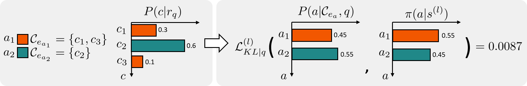
Figure 3: Concept regularizer. $P(a_{1}|\mathcal{C}_{e_{a_{1}}},q)=\text{exp}(0.3+0.1)/(\text{exp}(0.3+0.1)+\text{exp}(0.6))=0.45$. $P(a_{2}|\mathcal{C}_{e_{a_{2}}},q)=\text{exp}(0.6)/(\text{exp}(0.3+0.1)+\text{exp}(0.6))=0.55$.

$$P(a|\mathcal{C}_{e_{a}},q)=\frac{\text{exp}(\sum_{c\in\mathcal{C}_{e_{a}}}P(c|r_{q}))}{\sum_{a^{\prime}\in\mathcal{A}^{(l)}}\text{exp}(\sum_{c^{\prime}\in\mathcal{C}_{e_{a^{\prime}}}}P(c^{\prime}|r_{q}))}$$ (10)

We then compute the Kullback-Leibler (KL) divergence between $P(a|\mathcal{C}_{e_{a}},q)$ and $\pi(a|s^{(l)})$ and minimize it during parameter optimization.

$$\mathcal{L}_{\text{KL}|q}^{(l)}=\sum_{a\in\mathcal{A}^{(l)}}\pi(a|s^{(l)})\log\left(\frac{\pi(a|s^{(l)})}{P(a|\mathcal{C}_{e_{a}},q)}\right).$$ (11)

Note that $r_{q}\in\mathcal{R}$ is observable in $\mathcal{G}_{\text{back}}$. $\mathcal{G}_{\text{back}}$ is huge and contains a substantial number of facts of $r_{q}$. As stated in FILT [13], although we have only $K$ associated edges for each unseen entity $e^{\prime}$, its concepts $\mathcal{C}_{e^{\prime}}$ is known. Our concept regularizer enables a parameter-free approach to match the concept-aware action probability $P(a|\mathcal{C}_{e_{a}},q)$ with the action probability taken from the policy $\pi(a|s^{(l)})$. It can be taken as guiding the policy to conform to the distribution of $r_{q}$’s objects’ concepts observed in $\mathcal{G}_{\text{back}}$. We illustrate our concept regularizer in Fig. 3.

4.5 Parameter Learning

Following [13], we train FITCARL with episodic training. In each episode, a training task $T$ is sampled, where we sample a $Sup_{e^{\prime}}$ for every unseen entity $e^{\prime}\in\mathcal{E}^{\prime}_{\text{meta-train}}$ ($\mathcal{E}_{T}=\mathcal{E}^{\prime}_{\text{meta-train}}$) and calculate loss over $Que_{e^{\prime}}$. For each LP query $q$, we aim to maximize the cumulative reward along $L$ steps of search. We write our loss function (we minimize our loss) for each training task $T$ as follows.

$a^{(l)}$ is the selected action at search step $l$. $\gamma^{l}$ is the $l^{\text{th}}$ order of a discount factor $\gamma\in[0,1)$. $\eta$ is a hyperparameter deciding the magnitude of concept regularization. We use Algorithm 1 in Appendix E to further illustrate our meta-training process.

5 Experiments

We compare FITCARL with baselines on TKG few-shot OOG LP (Section 5.2). In Section 5.3.1, we first do several ablation studies to study the effectiveness of different model components. We then plot the performance over time to show FITCARL’s robustness and present a case study to show FITCARL’s explainability and the importance of learning confidence. We provide implementation details in Appendix A.

5.1 Experimental Setting

We do experiments on three datasets proposed in [13], i.e., ICEWS14-OOG, ICEWS18-OOG and ICEWS0515-OOG. They contain the timestamped political facts in 2014, 2018 and from 2005 to 2015, respectively. All of them are constructed by taking the facts from the ICEWS [6] TKB. Dataset statistics are shown in Table 1. We employ two evaluation metrics, i.e., mean reciprocal rank (MRR) and Hits@1/3/10. We provide detailed definitions of both metrics in Appendix D. We use the filtered setting proposed in [5] for fairer evaluation. For baselines, we consider the following methods. (1) Two traditional KGC methods, i.e., ComplEx [35] and BiQUE [14]. (2) Three traditional TKGC methods, i.e., TNTComplEx [20], TeLM [44], and TeRo [45]. (3) Three inductive KGC methods, i.e., MEAN [15], LAN [40], and GEN [3]. Among them, only GEN is trained with a meta-learning framework. (4) Two inductive TKG reasoning methods, including an inductive TKG forecasting method TITer [33], and a meta-learning-based inductive TKGC method FILT [13] (FILT is the only previous work developed to solve TKG few-shot OOG LP). We take the experimental results of all baselines (except TITer) from [13]. Following [13], we train TITer over all the TKG facts in $\mathcal{G}_{\text{back}}$ and $\mathbb{T}_{\text{meta-train}}$. We constrain TITer to only observe support quadruples of each test entity in $\mathcal{E}^{\prime}_{\text{meta-test}}$ for inductive learning during inference. All methods are tested over exactly the same test examples.

Table 1: Dataset statistics.

Dataset	$|\mathcal{E}|$	$|\mathcal{R}|$	$|\mathcal{T}|$	$|\mathcal{E}^{\prime}_{\text{meta-train}}|$	$|\mathcal{E}^{\prime}_{\text{meta-valid}}|$	$|\mathcal{E}^{\prime}_{\text{meta-test}}|$	$|\mathcal{G}_{\text{back}}|$	$|\mathbb{T}_{\text{meta-train}}|$	$|\mathbb{T}_{\text{meta-valid}}|$	$|\mathbb{T}_{\text{meta-test}}|$
ICEWS14-OOG	7128	230	365	385	48	49	83448	5772	718	705
ICEWS18-OOG	23033	256	304	1268	160	158	444269	19291	2425	2373
ICEWS0515-OOG	10488	251	4017	647	80	82	448695	10115	1217	1228

5.2 Main Results

Table 2 shows the experimental results of TKG 1-shot/3-shot OOG LP. We observe that traditional KGC and TKGC methods are beaten by inductive learning methods. It is because traditional methods cannot handle unseen entities. Besides, we also find that meta-learning-based methods, i.e., GEN, FILT and FITCARL, show better performance than other inductive learning methods. This is because meta-learning is more suitable for dealing with few-shot learning problems. FITCARL shows superior performance over all metrics on all datasets. It outperforms the previous stat-of-the-art FILT with a huge margin. We attribute it to several reasons. (1) Unlike FILT that uses KG score function over all the entities for prediction, FITCARL is an RL-based method that directly searches the predicted answer through their multi-hop temporal neighborhood, making it better capture highly-related graph information through time. (2) FITCARL takes advantage of its confidence learner. It helps to alleviate the negative impact from the few-shot setting. (3) Concept regularizer serves as a strong tool for exploiting concept-aware information in TKBs and adaptively guides FITCARL to learn a policy that conforms to the concept distribution shown in $\mathcal{G}_{\text{back}}$.

Table 2: Experimental results of TKG 1-shot and 3-shot OOG LP. Evaluation metrics are MRR and Hits@1/3/10 (H@1/3/10). Best results are marked bold.

Datasets	ICEWS14-OOG								ICEWS18-OOG								ICEWS0515-OOG
	MRR		H@1		H@3		H@10		MRR		H@1		H@3		H@10		MRR		H@1		H@3		H@10
Model	1-S	3-S	1-S	3-S	1-S	3-S	1-S	3-S	1-S	3-S	1-S	3-S	1-S	3-S	1-S	3-S	1-S	3-S	1-S	3-S	1-S	3-S	1-S	3-S
ComplEx	.048	.046	.018	.014	.045	.046	.099	.089	.039	.044	.031	.026	.048	.042	.085	.093	.077	.076	.045	.048	.074	.071	.129	.120
BiQUE	.039	.035	.015	.014	.041	.030	.073	.066	.029	.032	.022	.021	.033	.037	.064	.073	.075	.083	.044	.049	.072	.077	.130	.144
TNTComplEx	.043	.044	.015	.016	.033	.042	.102	.096	.046	.048	.023	.026	.043	.044	.087	.082	.034	.037	.014	.012	.031	.036	.060	.071
TeLM	.032	.035	.012	.009	.021	.023	.063	.077	.049	.019	.029	.001	.045	.013	.084	.054	.080	.072	.041	.034	.077	.072	.138	.151
TeRo	.009	.010	.002	.002	.005	.002	.015	.020	.007	.006	.003	.001	.006	.003	.013	.006	.012	.023	.000	.010	.008	.017	.024	.040
MEAN	.035	.144	.013	.054	.032	.145	.082	.339	.016	.101	.003	.014	.012	.114	.043	.283	.019	.148	.003	.039	.017	.175	.052	.384
LAN	.168	.199	.050	.061	.199	.255	.421	.500	.077	.127	.018	.025	.067	.165	.199	.344	.171	.182	.081	.068	.180	.191	.367	.467
GEN	.231	.234	.162	.155	.250	.284	.378	.389	.171	.216	.112	.137	.189	.252	.289	.351	.268	.322	.185	.231	.308	.362	.413	.507
TITer	.144	.200	.105	.148	.163	.226	.228	.314	.064	.115	.038	.076	.075	.131	.011	.186	.115	.228	.080	.168	.130	.262	.173	.331
FILT	.278	.321	.208	.240	.305	.357	.410	.475	.191	.266	.129	.187	.209	.298	.316	.417	.273	.370	.201	.299	.303	.391	.405	.516
FITCARL	.418	.481	.284	.329	.522	.646	.681	.696	.297	.370	.156	.193	.386	.559	.584	.627	.345	.513	.202	.386	.482	.618	.732	.700

5.3 Further Analysis

5.3.1 Ablation Study

We conduct several ablation studies to study the effectiveness of different model components. (A) Action Space Sampling Variants: To prevent oversized action space $\mathcal{A}^{(l)}$, we use a time-adaptive sampling method (see Section 4.2). We show its effectiveness by switching it to random sample (ablation A1) and time-proximity sample (ablation A2). In time-proximity sample, we take a fixed number of outgoing edges temporally closest to the current node at $t^{(l)}$ as $\mathcal{A}^{(l)}$. We keep $|\mathcal{A}^{(l)}|$ unchanged. (B) Removing Confidence Learner: In ablation B, we remove the confidence learner. (C) Removing Concept Regularizer: In ablation C, we remove concept regularizer. (D) Time-Aware Transformer Variants: We remove the time-aware positional encoding method by deleting the second term of Equation 2. (E) Removing Temporal Reasoning Modules: In ablation E, we study the importance of temporal reasoning. We first combine ablation A1 and D, and then delete every term related to time difference representations computed with Equation 1. We create a model variant without using any temporal information (see Appendix C for detailed setting). We present the experimental results of ablation studies in Table 3. From ablation A1 and A2, we observe that time-adaptive sample is effective. We also see a great performance drop in ablation B and C, indicating the strong importance of our confidence learner and concept regularizer. We only do ablation D for 3-shot model because in 1-shot case our model does not need to distinguish the importance of multiple support quadruples. We find that our time-aware positional encoding makes great contribution. Finally, we observe that ablation E shows poor performance (worse than A1 and D in most cases), implying that incorporating temporal information is essential for FITCARL to solve TKG few-shot OOG LP.

Table 3: Ablation study results. Best results are marked bold.

Datasets	ICEWS14-OOG								ICEWS18-OOG								ICEWS0515-OOG
	MRR		H@1		H@3		H@10		MRR		H@1		H@3		H@10		MRR		H@1		H@3		H@10
Model	1-S	3-S	1-S	3-S	1-S	3-S	1-S	3-S	1-S	3-S	1-S	3-S	1-S	3-S	1-S	3-S	1-S	3-S	1-S	3-S	1-S	3-S	1-S	3-S
A1	.404	.418	.283	.287	.477	.494	.647	.667	.218	.260	.153	.167	.220	.296	.404	.471	.190	.401	.108	.289	.196	.467	.429	.624
A2	.264	.407	.241	.277	.287	.513	.288	.639	.242	.265	.126	.168	.337	.291	.444	.499	.261	.414	.200	.267	.298	.545	.387	.640
B	.373	.379	.255	.284	.454	.425	.655	.564	.156	.258	.106	.191	.162	.271	.273	.398	.285	.411	.198	.336	.328	.442	.447	.567
C	.379	.410	.265	.236	.489	.570	.667	.691	.275	.339	.153	.190	.346	.437	.531	.556	.223	.411	.130	.243	.318	.544	.397	.670
D	-	.438	-	.262	-	.626	-	.676	-	.257	-	.160	-	.280	-	.500	-	.438	-	.262	-	.610	-	.672
E	.270	.346	.042	.178	.480	.466	.644	.662	.155	.201	.012	.117	.197	.214	.543	.429	.176	.378	.047	.239	.194	.501	.506	.584
FITCARL	.418	.481	.284	.329	.522	.646	.681	.696	.297	.370	.156	.193	.386	.559	.584	.627	.345	.513	.202	.386	.482	.618	.732	.700

5.3.2 Performance over Time

To demonstrate the robustness of FITCARL, we plot its MRR performance over prediction time (query time $t_{q}$). We compare FITCARL with two meta-learning-based strong baselines GEN and FILT. From Figure LABEL:fig:_ICEWS14-1 to LABEL:fig:_ICEWS05-15-3, we find that our model can constantly outperform baselines. This indicates that FITCARL improves LP performance for examples existing at almost all timestamps, proving its robustness. GEN is not designed for TKG reasoning, and thus it cannot show optimal performance. Although FILT is designed for TKG few-shot OOG LP, we show that our RL-based model is much stronger.

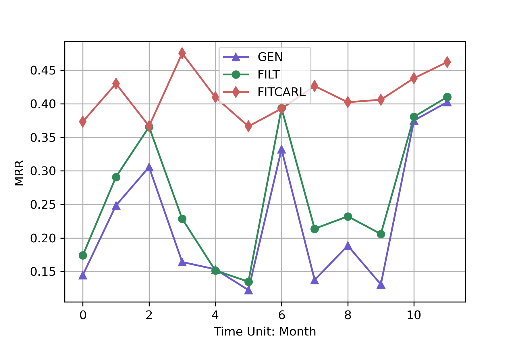
(a)

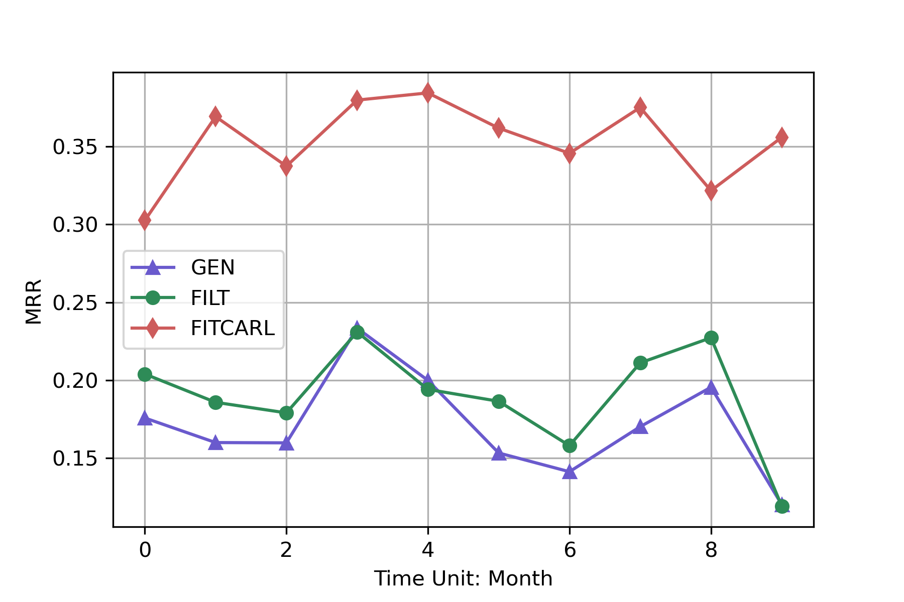
(b)

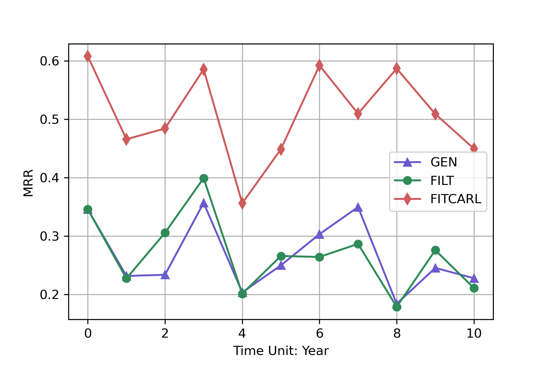
(c)

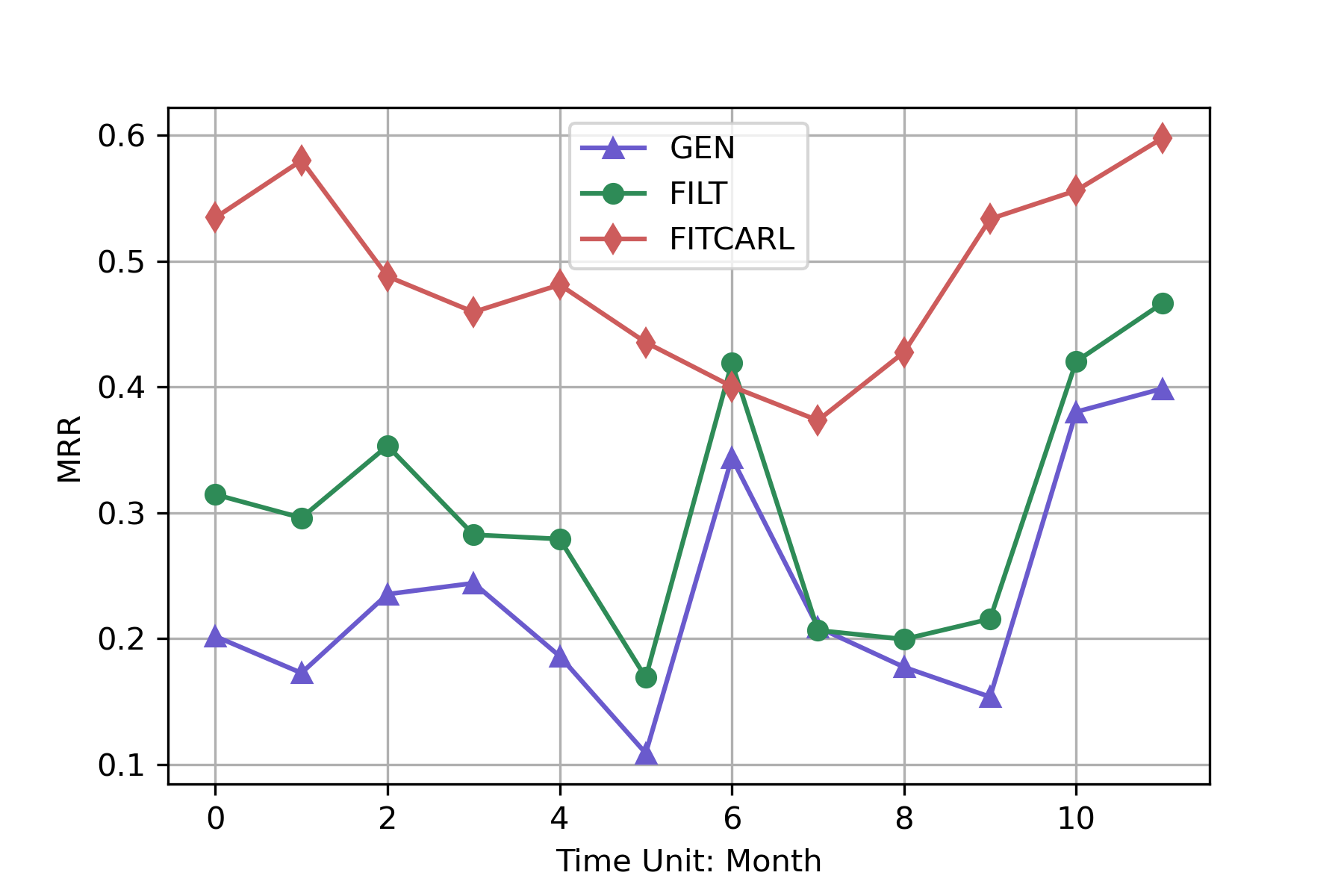
(d)

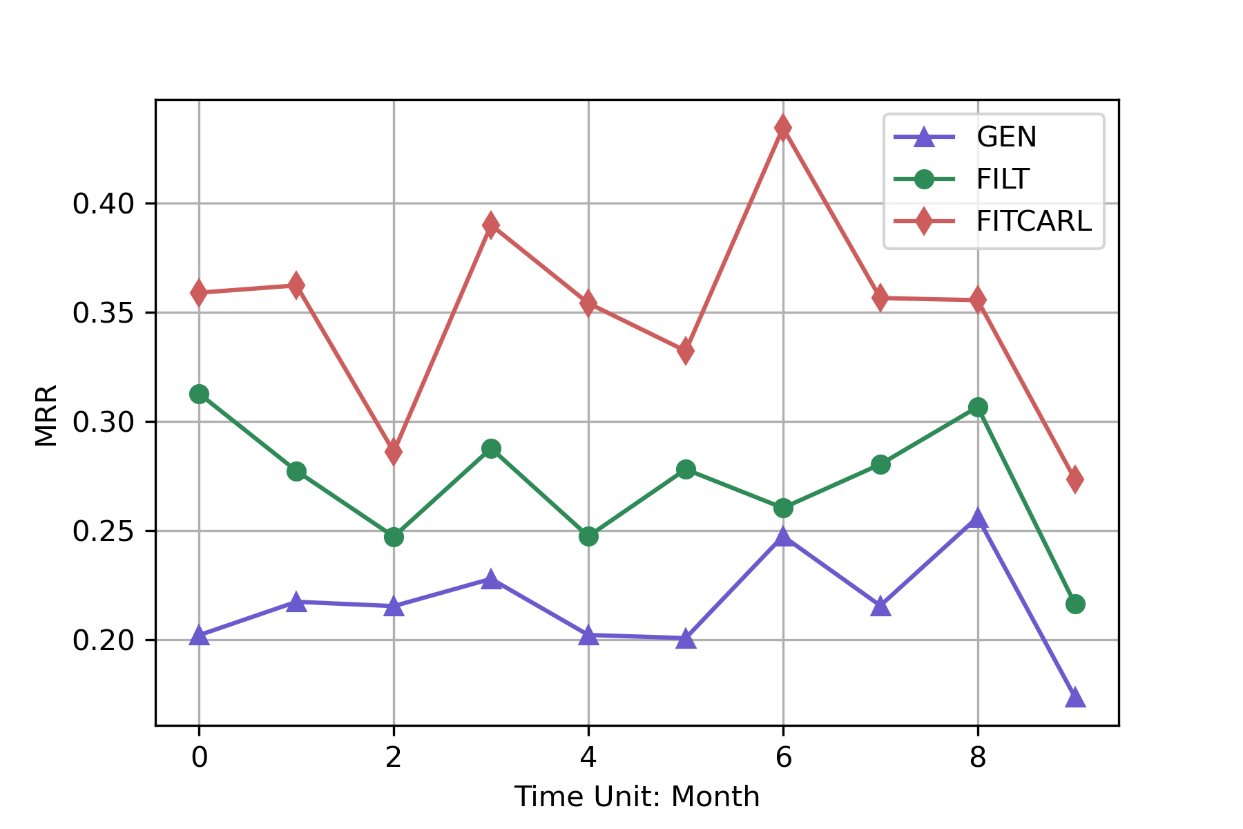
(e)

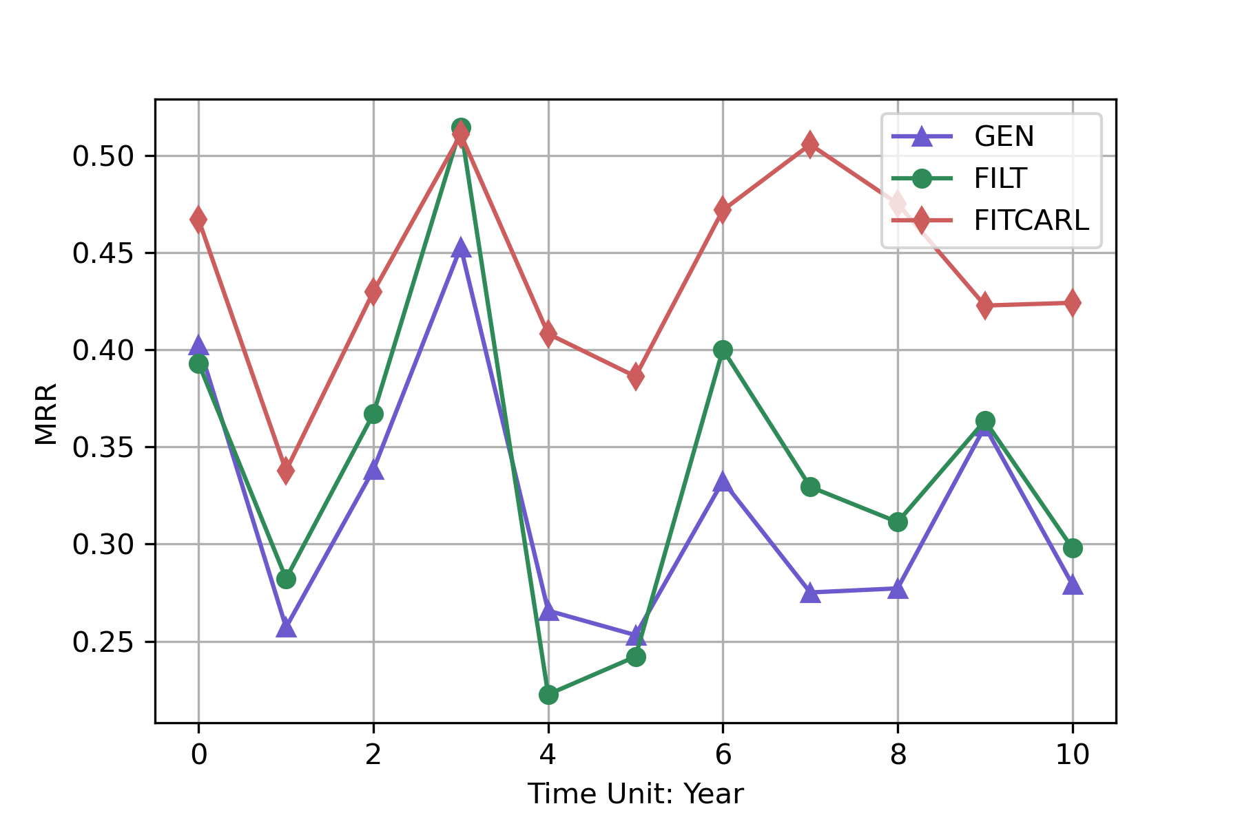
(f)

Figure 4: Performance comparison among FITCARL, FILT and GEN over different query time $t_{q}$. Horizontal axis of each subfigure denotes how temporally faraway from the first timestamp. We aggregate the performance of each month to one point in ICEWS14-OOG and ICEWS18-OOG. A point for ICEWS0515-OOG denotes the aggregated performance in each year.

5.3.3 Case Study

We do a case study to show how FITCARL provides explainability and how confidence learner helps in reasoning. We ask 3-shot FITCARL and its variant without the confidence learner (both trained on ICEWS14-OOG) to predict the missing entity of the LP query (Future Movement, Express intent to cooperate on intelligence, $?$, 2014-11-12), where Future Movement is a newly-emerged entity that is unseen during training and the answer to this LP query is Miguel Ángel Rodríguez. We visualize a specific reasoning path of each model and present them in Fig. 5. The relation Express intent to cooperate on intelligence indicates a positive relationship between subject and object entities. FITCARL performs a search with length $L=3$, where it finds an entity Military Personnel (Nigeria) that is in a negative relationship with both Future Movement and Miguel Ángel Rodríguez. FITCARL provides explanation by finding a reasoning path representing the proverb: The enemy of the enemy is my friend. For FITCARL without confidence learner, we find that it can also provide similar explanation by finding another entity that is also an enemy of Military Personnel (Nigeria). However, it fails to find the ground truth answer because it neglects the confidence of each action. The confidence learner assigns high probability to the ground truth entity, leading to a correct prediction.

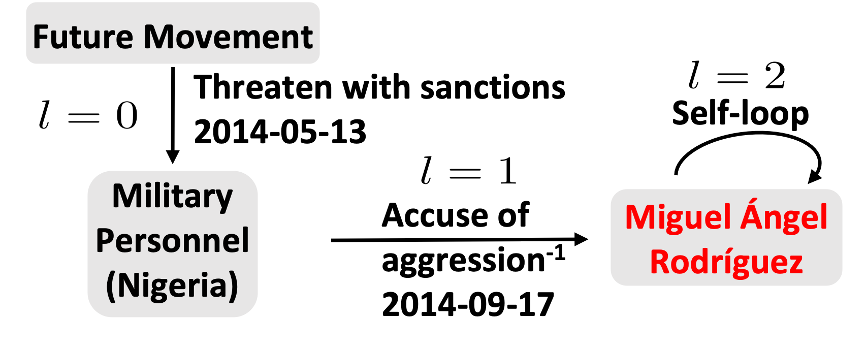
(a)

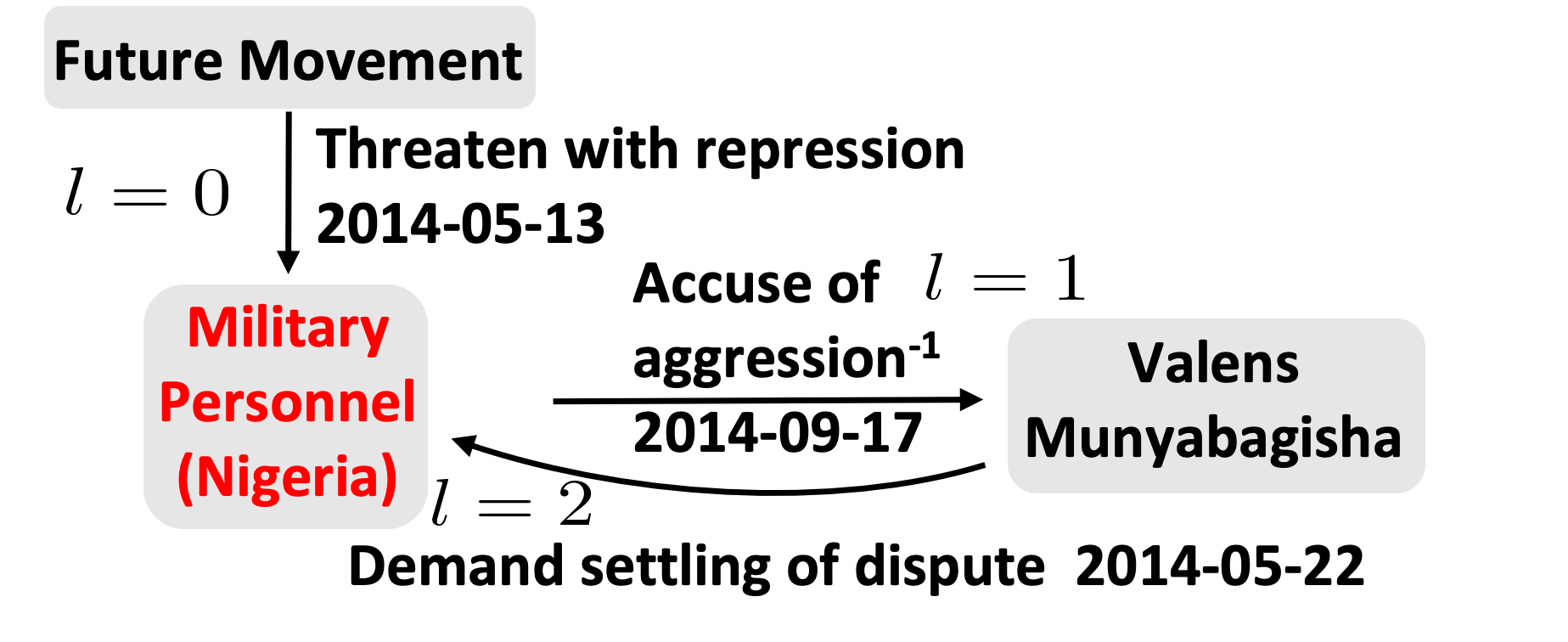
(b)

Figure 5: Case study reasoning path visualization. The entity marked in red are the answer predicted by the model. w.o. means without.

6 Conclusion

We present an RL-based TKGC method FITCARL to solve TKG few-shot OOG LP, where models are asked to predict the links concerning newly-emerged entities that have only a few observed associated facts. FITCARL is a meta-learning-based model trained with episodic training. It learns representations of newly-emerged entities by using a time-aware Transformer. To further alleviate the negative impact of the few-shot setting, a confidence learner is proposed to be coupled with the policy network for making better decisions. A parameter-free concept regularizer is also developed to better exploit concept-aware information in TKBs. Experimental results show that FITCARL achieves a new state-of-the-art and provides explainability.

Appendix 0.A Implementation Details

All experiments are implemented with PyTorch [28] on a single NVIDIA A40 with 48GB memory. We search hyperparameters following Table 4. For each dataset, we do 108 trials to try different hyperparameter settings. We run 1000 episodes for each trail and compare their meta-validation results. We choose the setting leading to the best meta-validation result and take it as the best hyperparameter setting. The best hyperparameter setting is reported in Table 5. Our time-aware Transformer uses two heads and two attention layers for all experiments. The results of FITCARL is the average of five runs. The GPU memory usage, training time and the number of parameters are presented in Table 6, 7 and 8, respectively. For all datasets, we use all meta-training entities $\mathcal{E}^{\prime}_{\text{meta-train}}$ as the considered unseen entities in each meta-training task $T$. This also applies during meta-validation and meta-test, where all the entities in $\mathcal{E}^{\prime}_{\text{meta-valid}}$/$\mathcal{E}^{\prime}_{\text{meta-test}}$ are considered appearing simultaneously in one evaluation task. All the datasets are taken from FILT’s official repository. We also take the pre-trained representations from it for our experiments. During evaluation, we follow previous RL-based TKG reasoning models TITer and CluSTeR and use beam search for answer searching. The beam size is 100 for all experiments.

We implement TITer with its official code. We give it the whole background graph $\mathcal{G}_{\text{back}}$ as well as all meta-training quadruples $\mathbb{T}_{\text{meta-train}}$ for training. During meta-validation and meta-test, it is further given support quadruples for predicting the query quadruples.

Table 4: Hyperparameter searching strategy.

Hyperparameter	Search Space
Embedding Size $d$	{100, 200}
Sampled Action Space Size	{25, 50, 100}
Search Step $L$	{3, 4}
Regularizer Coefficient $\eta$	{1e-11, 1e-9, 1e-7}
Margin of Reward $\theta$	{1, 5, 10}

Table 5: Best hyperparameter settings.

Datasets	ICEWS14-OOG	ICEWS18-OOG	ICEWS0515-OOG
Hyperparameter
Embedding Size $d$	100	100	100
Sampled Action Space Size	50	50	50
Search Step $L$	3	3	3
Regularizer Coefficient $\eta$	1e-9	1e-9	1e-9
Margin of Reward $\theta$	5	5	5

Table 6: GPU memory usage (MB).

Datasets	ICEWS14-OOG		ICEWS18-OOG		ICEWS0515-OOG
	GPU Memory		GPU Memory		GPU Memory
Model	1-S	3-S	1-S	3-S	1-S	3-S
FITCARL	10729	11153	14761	15419	14765	15475

Table 7: Training time (min).

Datasets	ICEWS14-OOG		ICEWS18-OOG		ICEWS0515-OOG
	Time		Time		Time
Model	1-S	3-S	1-S	3-S	1-S	3-S
FITCARL	225	85	305	764	1059	297

Table 8: Number of parameters.

Datasets	ICEWS14-OOG		ICEWS18-OOG		ICEWS0515-OOG
	# Param		# Param		# Param
Model	1-S	3-S	1-S	3-S	1-S	3-S
FITCARL	8271206	8271410	14633206	10006710	9615206	9615410

Appendix 0.B Difference between TKGC and TKG forecasting

Assume we have a TKG $\mathcal{G}=\{(s,r,o,t)|s,o\in\mathcal{E},r\in\mathcal{R},t\in\mathcal{T}\}\subseteq\mathcal{E}\times\mathcal{R}\times\mathcal{E}\times\mathcal{T}$, where $\mathcal{E}$, $\mathcal{R}$, $\mathcal{T}$ denote a finite set of entities, relations and timestamps, respectively. We define the TKG forecasting task (also known as TKG extrapolation) as follows. Assume we have an LP query $(s_{q},r_{q},?,t_{q})$ (or $(?,r_{q},o_{q},t_{q})$) derived from a query quadruple $(s_{q},r_{q},o_{q},t_{q})$. TKG forecasting aims to predict the missing entity in the LP query, given the observed past TKG facts $\mathcal{O}=\{(s_{i},r_{i},o_{i},t_{i})|t_{i}<t_{q}\}$. Such temporal restriction is not imposed in TKGC (also known as TKG interpolation), where the observed TKG facts from any timestamp, including $t_{q}$ and the timestamps after $t_{q}$, can be used for prediction.

TITer is designed for TKG forecasting, therefore it only performs its RL search process in the direction pointing at the past. This leads to a great loss of information along the whole time axis. TITer also does not use a meta-learning framework for adapting to the few-shot setting, which is also a reason for its weak performance on TKG few-shot OOG LP. Please refer to the papers studying TKG forecasting, e.g., [18, 16], for more details.

Appendix 0.C Ablation E Details

We describe here how we change equations in ablation E to build a model variant without using any temporal information. First, we change the action space sampling method to random sample, which corresponds to ablation A1. This means we do not use temporal information to compute time-adaptive sampling probabilities. Next, we neglect the last term in Equation 2 of the main paper. It thus becomes

$$\text{att}_{u,v}=\frac{\text{exp}(\alpha_{u,v})}{\sum_{k=1}^{K+1}\text{exp}(\alpha_{u,k})},$$ (13)

$$\alpha_{u,v}=\frac{1}{\sqrt{d}}(\mathbf{W}_{TrQ}\mathbf{h}_{u})^{\top}(\mathbf{W}_{TrK}\mathbf{h}_{v}),$$

which corresponds to ablation D. Finally, we remove every term in all equations containing time-difference representations. For a node $(e,t)$, its representation becomes $\mathbf{h}_{e}$. Thus, Equation 3 of the main paper becomes

$$\mathbf{h}_{\text{hist}^{(l)}}=\text{GRU}\left(\left(\mathbf{h}_{{r}^{(l)}}\|\mathbf{h}_{e^{(l)}}\right),\mathbf{h}_{\text{hist}^{(l-1)}}\right),$$ (14)

$$\mathbf{h}_{\text{hist}^{(0)}}=\text{GRU}\left(\left(\mathbf{h}_{{r}_{\text{dummy}}}\|\mathbf{h}_{e^{\prime}}\right),\mathbf{0}\right).$$

Equation 4 of the main paper becomes

$$\mathbf{h}_{\text{hist}^{(l)},q|a}=\text{att}_{\text{hist}^{(l)},a}\cdot\bar{\mathbf{h}}_{\text{hist}^{(l)}}+\text{att}_{q,a}\cdot\bar{\mathbf{h}}_{q},$$ (15)

$$\bar{\mathbf{h}}_{\text{hist}^{(l)}}={\mathbf{W}_{1}}^{\top}\mathbf{h}_{\text{hist}^{(l)}},\quad\bar{\mathbf{h}}_{q}={\mathbf{W}_{2}}^{\top}\left(\mathbf{h}_{r_{q}}\|\mathbf{h}_{e^{\prime}}\right).$$

Equation 5 and 6 of the main paper become

$$\text{att}_{\text{hist}^{(l)},a}=\frac{\text{exp}(\phi_{\text{hist}^{(l)},a})}{\text{exp}(\phi_{\text{hist}^{(l)},a})+\text{exp}(\phi_{q,a})},\text{att}_{q,a}=\frac{\text{exp}(\phi_{q,a})}{\text{exp}(\phi_{\text{hist}^{(l)},a})+\text{exp}(\phi_{q,a})},$$ (16)

where

$$\phi_{\text{hist}^{(l)},a}={\bar{\mathbf{h}}_{a}}^{\top}\bar{\mathbf{h}}_{\text{hist}^{(l)}},\ \phi_{q,a}={\bar{\mathbf{h}}_{a}}^{\top}\bar{\mathbf{h}}_{q},$$ (17)

$$\bar{\mathbf{h}}_{a}={\mathbf{W}_{3}}^{\top}\left(\mathbf{h}_{r_{a}}\|\mathbf{h}_{e_{a}}\right).$$

Equation 8 of the main paper becomes

$$\text{conf}_{a|q}=\frac{\text{exp}(\psi_{a|q})}{\sum_{a^{\prime}\in\mathcal{A}^{(l)}}\text{exp}(\psi_{a^{\prime}|q})},\ \text{where}\ \psi_{a|q}=\mathcal{W}\times_{1}\mathbf{h}_{e^{\prime}}\times_{2}\mathbf{h}_{r_{q}}\times_{3}\mathbf{h}_{e_{a}}.$$ (18)

The other equations remain unchanged. To this end, we create a model variant that uses no temporal information.

Appendix 0.D Evaluation Metrics

We use two evaluation metrics, i.e., mean reciprocal rank (MRR) and Hits@1/3/10. For every LP query $q$, we compute the rank $rank_{q}$ of the ground truth missing entity. We define MRR as: $\frac{1}{\sum_{e^{\prime}\in\mathcal{E}^{\prime}_{\text{meta-test}}}|Que_{e^{\prime}}|}\sum_{e^{\prime}\in\mathcal{E}^{\prime}_{\text{meta-test}}}\sum_{q\in Que_{e^{\prime}}}\frac{1}{rank_{q}}$. Hits@1/3/10 denote the proportions of the predicted links where ground truth missing entities are ranked as top 1, top3, top10, respectively. We also use the filtered setting proposed in [5] for fairer evaluation.

Appendix 0.E Meta-Training Algorithm of FITCARL

1

Input: Meta-training entities $\mathcal{E}^{\prime}_{\text{meta-train}}$, background TKG $\mathcal{G}_{\text{back}}$, shot size $K$

2

3for episode = 1: M do

4       for $e^{\prime}\in\mathcal{E}^{\prime}_{\text{meta-train}}$ do

5             Sample a support set $Sup_{e^{\prime}}$ and a query set $Que_{e^{\prime}}$

6            Learn meta-representations $\{\mathbf{h}_{e^{\prime}}^{i}\}_{i=1}^{K}$

7      for $e^{\prime}\in\mathcal{E}^{\prime}_{\text{meta-train}}$ do

8             for query $\in Que_{e^{\prime}}$ do

9                   Derive LP query $q$ from $query$

10                  Compute $\mathbf{h}_{e^{\prime}}$ using time-aware Transformer // Section 4.1

11                  Initialize $s^{(0)}\leftarrow(e^{\prime},t_{q},e^{\prime},r_{q},t_{q})$

12                  $\{R(s^{(l)},a^{(l)})\}_{l=0}^{L-1},\{\mathcal{L}_{\text{KL}|q}^{(l)}\}_{l=0}^{L-1},\{\pi(a^{(l)}|s^{(l)})\}_{l=0}^{L-1}\leftarrow$ Search$(L,s^{(0)})$

13            

14      

15      Compute loss $\mathcal{L}_{T}$ // Equation 12

16      Update model parameters using gradient of $\bigtriangledown\mathcal{L}_{T}$

17

18Procedure Search$(L,s^{(0)})$

19       for l = 0:L-1 do

20             Sample action space $\mathcal{A}^{(l)}$ from all observed outgoing edges of node $(e^{(l)},t^{(l)})$

21            Compute $P(a|s^{(l)},\text{hist}^{(l)})$ and $\text{conf}_{a|q}$ for $a\in\mathcal{A}^{(l)}$ // Equation 7, 8

22            Compute $\pi(a|s^{(l)})$ for each $a\in\mathcal{A}^{(l)}$ // Equation 9

23            Compute $\mathcal{L}_{\text{KL}|q}^{(l)}$ // Equation 11

24            Sample $a^{(l)}=(e_{a^{(l)}},r_{a^{(l)}},t_{a^{(l)}})$ according to policy $\pi$

25            Compute reward $R(s^{(l)},a^{(l)})$

26            Execute $a^{(l)}$, agent transfers to state $s^{(l+1)}=(e^{(l+1)},r^{(l+1)},e^{\prime},r_{q},t_{q})$

27      return $\{R(s^{(l)},a^{(l)})\}_{l=0}^{L-1},\{\mathcal{L}_{\text{KL}|q}^{(l)}\}_{l=0}^{L-1},\{\pi(a^{(l)}|s^{(l)})\}_{l=0}^{L-1}$

28      

Algorithm 1 FITCARL Meta-Training

We train FITCARL with episodic training. We present our meta-training process in Algorithm 1.

References

- [1] Abboud, R., Ceylan, İ.İ., Lukasiewicz, T., Salvatori, T.: Boxe: A box embedding model for knowledge base completion. In: NeurIPS (2020)
- [2] Ammanabrolu, P., Hausknecht, M.J.: Graph constrained reinforcement learning for natural language action spaces. In: ICLR. OpenReview.net (2020)
- [3] Baek, J., Lee, D.B., Hwang, S.J.: Learning to extrapolate knowledge: Transductive few-shot out-of-graph link prediction. In: NeurIPS (2020)
- [4] Balazevic, I., Allen, C., Hospedales, T.M.: Tucker: Tensor factorization for knowledge graph completion. In: EMNLP/IJCNLP (1). pp. 5184–5193. Association for Computational Linguistics (2019)
- [5] Bordes, A., Usunier, N., García-Durán, A., Weston, J., Yakhnenko, O.: Translating embeddings for modeling multi-relational data. In: NIPS. pp. 2787–2795 (2013)
- [6] Boschee, E., Lautenschlager, J., O’Brien, S., Shellman, S., Starz, J., Ward, M.: ICEWS Coded Event Data (2015)
- [7] Chen, K., Wang, Y., Li, Y., Li, A.: Rotateqvs: Representing temporal information as rotations in quaternion vector space for temporal knowledge graph completion. In: ACL (1). pp. 5843–5857. Association for Computational Linguistics (2022)
- [8] Chen, M., Zhang, W., Zhang, W., Chen, Q., Chen, H.: Meta relational learning for few-shot link prediction in knowledge graphs. In: EMNLP/IJCNLP (1). pp. 4216–4225. Association for Computational Linguistics (2019)
- [9] Cho, K., van Merrienboer, B., Gülçehre, Ç., Bahdanau, D., Bougares, F., Schwenk, H., Bengio, Y.: Learning phrase representations using RNN encoder-decoder for statistical machine translation. In: EMNLP. pp. 1724–1734. ACL (2014)
- [10] Ding, Z., He, B., Ma, Y., Han, Z., Tresp, V.: Learning meta representations of one-shot relations for temporal knowledge graph link prediction. CoRR abs/2205.10621 (2022)
- [11] Ding, Z., Ma, Y., He, B., Han, Z., Tresp, V.: A simple but powerful graph encoder for temporal knowledge graph completion. In: NeurIPS 2022 Temporal Graph Learning Workshop
- [12] Ding, Z., Qi, R., Li, Z., He, B., Wu, J., Ma, Y., Meng, Z., Han, Z., Tresp, V.: Forecasting question answering over temporal knowledge graphs. CoRR abs/2208.06501 (2022)
- [13] Ding, Z., Wu, J., He, B., Ma, Y., Han, Z., Tresp, V.: Few-shot inductive learning on temporal knowledge graphs using concept-aware information. In: 4th Conference on Automated Knowledge Base Construction (2022)
- [14] Guo, J., Kok, S.: Bique: Biquaternionic embeddings of knowledge graphs. In: EMNLP (1). pp. 8338–8351. Association for Computational Linguistics (2021)
- [15] Hamaguchi, T., Oiwa, H., Shimbo, M., Matsumoto, Y.: Knowledge transfer for out-of-knowledge-base entities : A graph neural network approach. In: IJCAI. pp. 1802–1808. ijcai.org (2017)
- [16] Han, Z., Ding, Z., Ma, Y., Gu, Y., Tresp, V.: Learning neural ordinary equations for forecasting future links on temporal knowledge graphs. In: EMNLP (1). pp. 8352–8364. Association for Computational Linguistics (2021)
- [17] He, Y., Wang, Z., Zhang, P., Tu, Z., Ren, Z.: VN network: Embedding newly emerging entities with virtual neighbors. In: CIKM. pp. 505–514. ACM (2020)
- [18] Jin, W., Zhang, C., Szekely, P.A., Ren, X.: Recurrent event network for reasoning over temporal knowledge graphs. CoRR abs/1904.05530 (2019)
- [19] Jung, J., Jung, J., Kang, U.: Learning to walk across time for interpretable temporal knowledge graph completion. In: KDD. pp. 786–795. ACM (2021)
- [20] Lacroix, T., Obozinski, G., Usunier, N.: Tensor decompositions for temporal knowledge base completion. In: ICLR. OpenReview.net (2020)
- [21] Leblay, J., Chekol, M.W.: Deriving validity time in knowledge graph. In: WWW (Companion Volume). pp. 1771–1776. ACM (2018)
- [22] Li, J., Tang, T., Zhao, W.X., Wei, Z., Yuan, N.J., Wen, J.: Few-shot knowledge graph-to-text generation with pretrained language models. In: ACL/IJCNLP (Findings). Findings of ACL, vol. ACL/IJCNLP 2021, pp. 1558–1568. Association for Computational Linguistics (2021)
- [23] Li, Z., Jin, X., Guan, S., Li, W., Guo, J., Wang, Y., Cheng, X.: Search from history and reason for future: Two-stage reasoning on temporal knowledge graphs. In: ACL/IJCNLP (1). pp. 4732–4743. Association for Computational Linguistics (2021)
- [24] Lin, Y., Liu, Z., Sun, M., Liu, Y., Zhu, X.: Learning entity and relation embeddings for knowledge graph completion. In: AAAI. pp. 2181–2187. AAAI Press (2015)
- [25] Messner, J., Abboud, R., Ceylan, İ.İ.: Temporal knowledge graph completion using box embeddings. In: AAAI. pp. 7779–7787. AAAI Press (2022)
- [26] Mirtaheri, M., Rostami, M., Ren, X., Morstatter, F., Galstyan, A.: One-shot learning for temporal knowledge graphs. In: 3rd Conference on Automated Knowledge Base Construction (2021)
- [27] Nickel, M., Tresp, V., Kriegel, H.: A three-way model for collective learning on multi-relational data. In: ICML. pp. 809–816. Omnipress (2011)
- [28] Paszke, A., Gross, S., Massa, F., Lerer, A., Bradbury, J., Chanan, G., Killeen, T., Lin, Z., Gimelshein, N., Antiga, L., Desmaison, A., Köpf, A., Yang, E.Z., DeVito, Z., Raison, M., Tejani, A., Chilamkurthy, S., Steiner, B., Fang, L., Bai, J., Chintala, S.: Pytorch: An imperative style, high-performance deep learning library. In: NeurIPS. pp. 8024–8035 (2019)
- [29] Sadeghian, A., Armandpour, M., Colas, A., Wang, D.Z.: Chronor: Rotation based temporal knowledge graph embedding. In: AAAI. pp. 6471–6479. AAAI Press (2021)
- [30] Saxena, A., Tripathi, A., Talukdar, P.P.: Improving multi-hop question answering over knowledge graphs using knowledge base embeddings. In: ACL. pp. 4498–4507. Association for Computational Linguistics (2020)
- [31] Schlichtkrull, M.S., Kipf, T.N., Bloem, P., van den Berg, R., Titov, I., Welling, M.: Modeling relational data with graph convolutional networks. In: ESWC. Lecture Notes in Computer Science, vol. 10843, pp. 593–607. Springer (2018)
- [32] Sheng, J., Guo, S., Chen, Z., Yue, J., Wang, L., Liu, T., Xu, H.: Adaptive attentional network for few-shot knowledge graph completion. In: EMNLP (1). pp. 1681–1691. Association for Computational Linguistics (2020)
- [33] Sun, H., Zhong, J., Ma, Y., Han, Z., He, K.: Timetraveler: Reinforcement learning for temporal knowledge graph forecasting. In: EMNLP (1). pp. 8306–8319. Association for Computational Linguistics (2021)
- [34] Tresp, V., Esteban, C., Yang, Y., Baier, S., Krompaß, D.: Learning with memory embeddings. arXiv preprint arXiv:1511.07972 (2015)
- [35] Trouillon, T., Welbl, J., Riedel, S., Gaussier, É., Bouchard, G.: Complex embeddings for simple link prediction. In: ICML. JMLR Workshop and Conference Proceedings, vol. 48, pp. 2071–2080. JMLR.org (2016)
- [36] Tucker, L.R.: The extension of factor analysis to three-dimensional matrices. In: Gulliksen, H., Frederiksen, N. (eds.) Contributions to mathematical psychology., pp. 110–127. Holt, Rinehart and Winston, New York (1964)
- [37] Vashishth, S., Sanyal, S., Nitin, V., Talukdar, P.P.: Composition-based multi-relational graph convolutional networks. In: ICLR. OpenReview.net (2020)
- [38] Vaswani, A., Shazeer, N., Parmar, N., Uszkoreit, J., Jones, L., Gomez, A.N., Kaiser, L., Polosukhin, I.: Attention is all you need. In: NIPS. pp. 5998–6008 (2017)
- [39] Vinyals, O., Blundell, C., Lillicrap, T., Kavukcuoglu, K., Wierstra, D.: Matching networks for one shot learning. In: NIPS. pp. 3630–3638 (2016)
- [40] Wang, P., Han, J., Li, C., Pan, R.: Logic attention based neighborhood aggregation for inductive knowledge graph embedding. In: AAAI. pp. 7152–7159. AAAI Press (2019)
- [41] Wang, R., Li, Z., Sun, D., Liu, S., Li, J., Yin, B., Abdelzaher, T.F.: Learning to sample and aggregate: Few-shot reasoning over temporal knowledge graphs. In: NeurIPS (2022)
- [42] Wu, J., Cao, M., Cheung, J.C.K., Hamilton, W.L.: Temp: Temporal message passing for temporal knowledge graph completion. In: EMNLP (1). pp. 5730–5746. Association for Computational Linguistics (2020)
- [43] Xiong, W., Yu, M., Chang, S., Guo, X., Wang, W.Y.: One-shot relational learning for knowledge graphs. In: EMNLP. pp. 1980–1990. Association for Computational Linguistics (2018)
- [44] Xu, C., Chen, Y., Nayyeri, M., Lehmann, J.: Temporal knowledge graph completion using a linear temporal regularizer and multivector embeddings. In: NAACL-HLT. pp. 2569–2578. Association for Computational Linguistics (2021)
- [45] Xu, C., Nayyeri, M., Alkhoury, F., Yazdi, H.S., Lehmann, J.: Tero: A time-aware knowledge graph embedding via temporal rotation. In: COLING. pp. 1583–1593. International Committee on Computational Linguistics (2020)
- [46] Yang, B., Yih, W., He, X., Gao, J., Deng, L.: Embedding entities and relations for learning and inference in knowledge bases. In: ICLR (Poster) (2015)
- [47] Zhang, F., Zhang, Z., Ao, X., Zhuang, F., Xu, Y., He, Q.: Along the time: Timeline-traced embedding for temporal knowledge graph completion. In: CIKM. pp. 2529–2538. ACM (2022)
- [48] Zhang, Y., Dai, H., Kozareva, Z., Smola, A.J., Song, L.: Variational reasoning for question answering with knowledge graph. In: AAAI. pp. 6069–6076. AAAI Press (2018)