High Probability and Risk-Averse Guarantees
for a Stochastic Accelerated Primal-Dual Method

Abstract

We consider stochastic strongly-convex-strongly-concave (SCSC) saddle point (SP) problems which frequently arise in applications ranging from distributionally robust learning to game theory and fairness in machine learning. We focus on the recently developed stochastic accelerated primal-dual algorithm (SAPD), which admits optimal complexity in several settings as an accelerated algorithm. We provide high probability guarantees for convergence to a neighborhood of the saddle point that reflects accelerated convergence behavior. We also provide an analytical formula for the limiting covariance matrix of the iterates for a class of stochastic SCSC quadratic problems where the gradient noise is additive and Gaussian. This allows us to develop lower bounds for this class of quadratic problems which show that our analysis is tight in terms of the high probability bound dependency to the parameters. We also provide a risk-averse convergence analysis characterizing the “Conditional Value at Risk”, the “Entropic Value at Risk”, and the $\chi^{2}$-divergence of the distance to the saddle point, highlighting the trade-offs between the bias and the risk associated with an approximate solution obtained by terminating the algorithm at any iteration.

1 Introduction

We consider strongly convex/strongly concave (SCSC) saddle point problems of the form:

$$\min_{x\in\operatorname{\mathcal{X}}}\max_{y\in\operatorname{\mathcal{Y}}}\operatorname{\mathcal{L}}(x,y)\triangleq f(x)+\operatorname{\Phi}(x,y)-g(y),$$ (1.1)

where $\mathcal{X}$ and $\mathcal{Y}$ are finite-dimensional Euclidean spaces, $f:\mathcal{X}\to\mathbb{R}{\color[rgb]{0,0,0}\cup\{+\infty\}}$ and $g:\mathcal{Y}\times\mathbb{R}{\color[rgb]{0,0,0}\cup\{+\infty\}}$ are closed convex functions, and $\Phi:\mathcal{X}\times\mathcal{Y}\to\mathbb{R}$ is a smooth convex-concave function such that $\mathcal{L}(x,y)$ is strongly convex in $x$ and strongly concave in $y$, i.e., SCSC – see Assumption 1 for details. Throughout the paper, we assume that $f$ and $g$ are strongly convex; since $\mathcal{L}$ is SCSC, we emphasize that this assumption is without loss of generality as strong convexity/concavity can be transferred from $\Phi$ to $f$ and $g$ by adding and subtracting simple quadratics.

Such saddle point (SP) problems arise in many applications and different contexts. In unconstrained and constrained optimization problems, saddle-point formulations arise naturally when the problems are reformulated as a minimax problem based on the Lagrangian duality. Furthermore, the SP formulation in (1.1) encompasses many key problems such as robust optimization (Ben-Tal et al., 2009) – here $g$ is selected to be the indicator function of an uncertainty set from which nature (adversary) picks an uncertain model parameter $y$, and the objective is to choose $x\in\mathcal{X}$ that minimizes the worst-case cost $\max_{y\in\mathcal{Y}}\mathcal{L}(x,y)$, i.e., a two-player zero-sum game. Other applications involving SCSC problems include but are not limited to supervised learning with non-separable regularizers (where $\Phi(x,y)$ may not be bilinear) (Palaniappan and Bach, 2016), fairness in machine learning (Liu et al., 2022), unsupervised learning (Palaniappan and Bach, 2016) and various image processing problems, e.g., denoising, (Chambolle and Pock, 2011).

In this work, we are interested in SCSC problems where the partial gradients $\nabla_{x}\Phi$ and $\nabla_{y}\Phi$ are not deterministically available; but, instead we postulate that their stochastic estimates $\widetilde{\nabla}_{x}\Phi$ and $\widetilde{\nabla}_{y}\Phi$ are accessible. Such a setting arises frequently in large-scale optimization and machine learning applications where the gradients are estimated from either streaming data or from random samples of data (see e.g. (Zhu et al., 2023; Gürbüzbalaban et al., 2022; Bottou et al., 2018)). First-order (FO) methods that rely on stochastic estimates of the gradient information have been the leading computational approach for computing low-to-medium-accuracy solutions for these problems because of their cheap iterations and mild dependence on the problem dimension and data size. In this paper, our focus will be on first-order primal-dual algorithms that rely on stochastic gradient estimates for solving (1.1).

Existing relevant work.

Stochastic primal-dual algorithms for solving SP problems generate a sequence of primal and dual iterate pairs $z_{n}=(x_{n},y_{n})\in\mathcal{X}\times\mathcal{Y}\triangleq\mathcal{Z}$ starting from an initial point $(x_{0},y_{0})\in\operatorname{\mathbf{dom}}f\times\operatorname{\mathbf{dom}}g\triangleq Z$. Two popular metrics to assess the quality of a random solution $(\hat{x},\hat{y})$ returned by a stochastic algorithm are the expected gap and the expected squared distance defined as

$$\mathcal{G}(\hat{x},\hat{y})\triangleq\mathbb{E}\big{[}\sup_{(x,y)\in\mathcal{X}\times\mathcal{Y}}\big{\{}\mathcal{L}(\hat{x},y)-\mathcal{L}(x,{\color[rgb]{0,0,0}\hat{y}})\big{\}}\big{]},\quad{\mathcal{D}(\hat{x},\hat{y})\triangleq\mathbb{E}[\|\hat{x}-\operatorname{x^{\star}}\|^{2}+\|\hat{y}-\operatorname{y^{\star}}\|^{2}]},$$ (1.2)

respectively, where $(\operatorname{x^{\star}},\operatorname{y^{\star}})$ denotes the unique saddle point of (1.1), due to the strong convexity of $f$ and $g$. The iteration complexity of FO-methods in these two metrics depend naturally on the block Lipschitz constants $L_{xx}$, $L_{xy}$, $L_{yy}$ and $L_{yx}$, i.e., Lipschitz constants of $\nabla_{x}\Phi(\cdot,y)$, $\nabla_{x}\Phi(x,\cdot)$, $\nabla_{y}\Phi(x,\cdot)$ and $\nabla_{y}\Phi(\cdot,y)$ as well as on the strong convexity constants $\mu_{x}$ and $\mu_{y}$ of the functions $f$ and $g$. In particular, Fallah et al. (2020) show that a multi-stage variant of Stochastic Gradient Descent Ascent (SGDA) algorithm generates $(x_{\epsilon},y_{\epsilon})$ such that $\mathcal{D}(x_{\epsilon},y_{\epsilon})\leq\epsilon$ within $\mathcal{O}(\kappa^{2}\ln(1/\epsilon)+\frac{\delta^{2}}{{\mu^{2}}}\frac{1}{\epsilon})$ gradient oracle calls, where $\delta^{2}=\max{\color[rgb]{0,0,0}\{}\delta_{x}^{2},\delta_{y}^{2}{\color[rgb]{0,0,0}\}}$, while $\delta_{x}^{2}$ and $\delta_{y}^{2}$ are bounds on the variance of the stochastic gradients $\widetilde{\nabla}_{x}\Phi$ and $\widetilde{\nabla}_{y}\Phi$, respectively; $\mu\triangleq\min\{\mu_{x},\mu_{y}\}$ and $L\triangleq\max\{L_{xx},{\color[rgb]{0,0,0}L_{xy},L_{yx}},L_{yy}\}$ are the worst-case strong convexity and Lipschitz constants and $\kappa\triangleq L/\mu$ is defined as the condition number. SGDA analyzed in (Fallah et al., 2020) consists of Jacobi-type updates in the sense that stochastic gradient descent and ascent steps are taken simultaneously. Jacobi-type updates are easier to analyze than Gauss-Seidel updates in general, and can be viewed as solving a structured variational inequality (VI) problem, for which there are many existing techniques that directly apply, e.g., (Gidel et al., 2018; Chen et al., 2017). Zhang et al. (2022) consider deterministic SCSC problems, when gradient descent ascent (GDA) with Gauss-Seidel-type updates is considered, i.e., the primal and dual variables are updated in an alternating fashion using the most recent information obtained from the previous update step. Their results show that an accelerated asymptotic convergence rate, i.e., iteration complexity scales linearly with $\kappa$ instead of $\kappa^{2}$, can be obtained for the Gauss-Seidel variant of GDA. However, as discussed in (Zhang et al., 2022), this comes with the price that Gauss-Seidel style updates greatly complicate the analysis because every iteration of an alternating algorithm is a composition of two half updates. Furthermore, extending the acceleration result to non-asymptotic rates requires using momentum terms in either the primal or the dual updates, and this further complicates the convergence analysis. Fallah et al. (2020) also considered using momentum terms both in the primal and dual updates, and show that the multi-stage Stochastic Optimistic Gradient Descent Ascent (OGDA) algorithm using Jacobi-type updates achieves an iteration complexity of $\mathcal{O}(\kappa\ln(1/\epsilon)+\frac{\delta^{2}}{{\color[rgb]{0,0,0}\mu^{2}}\epsilon})$ in expected squared distance. There are also several other algorithms that can achieve the accelerated rate, i.e., $\log(1/\epsilon)$ has the coefficient $\kappa$ instead of $\kappa^{2}$ - see, e.g. (Beznosikov et al., 2022). We call this term that depend on the condition number as initialization bias since it captures how fast the error due to initial conditions decay and reflects the behavior of the algorithm in the noiseless setting. Among the algorithms that achieve an accelerated rate, the most closely related work to ours is (Zhang et al., 2023) which develops a stochastic accelerated primal-dual (SAPD) algorithm with Gauss-Seidel type updates. SAPD using a momentum acceleration only in the dual variable can generate $(x_{\epsilon},y_{\epsilon})$ such that $\mathbb{E}[\mu_{x}\|x_{\epsilon}-\operatorname{x^{\star}}\|^{2}+\mu_{y}\|y_{\epsilon}-\operatorname{y^{\star}}\|^{2}]\leq\epsilon$ within $\mathcal{O}\Big{(}\Big{(}\frac{L_{xx}}{\mu_{x}}+\frac{L_{yx}}{\sqrt{\mu_{x}\mu_{y}}}+\frac{L_{yy}}{\mu_{y}}+\Big{(}\frac{\delta_{x}^{2}}{{\mu_{x}}}+\frac{\delta_{y}^{2}}{{\mu_{y}}}\Big{)}\frac{1}{\epsilon}\Big{)}\log(\frac{1}{\varepsilon})\Big{)}$ iterations; this result implies ${\tilde{\mathcal{O}}(\kappa\ln(\varepsilon^{-1})+{\color[rgb]{0,0,0}\mu^{-2}}\delta^{2}\varepsilon^{-1})}$ in expected squared distance. This complexity is optimal for bilinear problems. To our knowledge, SAPD is also the fastest single-loop algorithm for solving stochastic SCSC problems in the form of (1.1) that are non-bilinear. Furthermore, using acceleration only in one update, as opposed to in both variables (Fallah et al., 2020), leads to smaller variance accumulation (see Zhang et al. (2023) for more details).

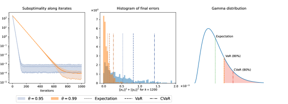
Figure 1: (Left) Convergence of SAPD on the saddle point problem $\min_{x\in\mathbb{R}}\max_{y\in\mathbb{R}}x^{2}/2+xy+y^{2}/2$, initialized at $x_{0}=y_{0}=10$ with momentum parameters $\theta=0.95$ and $\theta=0.99$. (Middle) Histogram of the distribution of the SAPD iterates $(x_{n},y_{n})$ after $n=1000$ iterations for 500 runs, with corresponding momentum parameters $\theta=0.95$ and $\theta=0.99$. (Right) Illustration of the expectation $\mathbb{E}(X)$, $p$-th quantile ($\mbox{VaR}_{1-p}(X)$) and $\mbox{CVaR}_{p}(X)$ of a gamma distributed random variable $X$ with shape parameter $3$ and scale parameter $5$ for $p=80\%$.

While the aforementioned results provide performance guarantees in expectation based on the metrics defined in (1.2) and their variants, unfortunately having guarantees in these metrics do not allow us to control tail events, i.e., the expected gap and distance can be smaller than a given target threshold $\varepsilon>0$; but, the iterates can still be arbitrarily far away from the saddle point with a non-zero probability. In this context, high probability guarantees are key in the sense that they allow us to control tail probabilities and quantify how many iterations are needed for the iterates to be in a neighborhood of the saddle point with a given probability level $p\in(0,1)$. This is illustrated on the right panel of Figure 1 where we run the SAPD algorithm for two different values of the momentum parameter $\theta=0.95$ and $\theta=0.99$ for a toy problem $\min_{x\in\mathbb{R}}\max_{y\in\mathbb{R}}\frac{1}{2}x^{2}+xy+\frac{1}{2}y^{2}$ with strong convexity parameters $\mu_{x}=\mu_{y}=1$ admitting a saddle point at $\operatorname{x^{\star}}=\operatorname{y^{\star}}=0$. SAPD is initialized at $(x_{0},y_{0})=(10,10)$, primal and dual stepsizes are chosen according to the Chambolle-Pock parametrization as suggested in (Zhang et al., 2023). For simplicity, the stochastic gradients $\widetilde{\nabla}_{x}\Phi$ and $\widetilde{\nabla}_{y}\Phi$ are set to $\nabla_{x}\Phi$ and $\nabla_{y}\Phi$ perturbed with additive i.i.d. Gaussian $\mathcal{N}(0,0.1)$ noise, and we assume that $\widetilde{\nabla}_{x}\Phi$ and $\widetilde{\nabla}_{y}\Phi$ are independent from each other and also from the past history of the algorithm. For each parameter choice, we run SAPD for 500 runs, and for $n=1000$ iterations for every run –see Figure 1 (Left), and plot the distribution of the squared distance of $(x_{n},y_{n})$ to the unique saddle point $(\operatorname{x^{\star}},\operatorname{y^{\star}})$, i.e., $E_{n}\triangleq{\color[rgb]{0,0,0}\|x_{n}-\operatorname{x^{\star}}\|^{2}+\|y_{n}-\operatorname{y^{\star}}\|^{2}}$, in Figure 1 (Middle). As we can see, the random error $E_{n}$ can take significantly larger values than its expectation $\mathcal{D}(x_{n},y_{n})=\mathbb{E}[E_{n}]$. This motivates estimating the $p$-th quantile of the error $E_{n}$, which is also called the value at risk at level $p$, traditionally abbreviated as $\operatorname{VaR}_{p}(E_{n})$ in the financial literature. While $\operatorname{VaR}_{p}(E_{n})$ represents a worst-case error $E_{n}$ associated with a probability $p$, it does not capture the behavior if that worst-case threshold is ever crossed. Conditional value at risk (CVaR) at level $p$, on the other hand, is an alternative risk measure that can be used characterizing the expected error if that worst-case threshold is ever crossed. CVaR is in fact a coherent risk measure with some desirable properties (Rockafellar and Royset, 2013). In Fig. 1(Middle), we report $\operatorname{VaR}_{p}(E_{n})$ and $\operatorname{CVaR}_{p}(E_{n})$ for $p=80\%$ and $n=1000$. We can see that $\operatorname{VaR}$ and $\operatorname{CVaR}$ capture the tail behavior better compared to expectation. Similar behavior can be seen on other distributions, e.g., in Figure 1(Right), we illustrate the expectation, $\operatorname{VaR}_{p}$, i.e., $p$-th quantile, and $\operatorname{CVaR}_{p}$ of a gamma-distributed random variable with shape parameter $3$, and scale parameter $5$ corresponding to $p=\%80$. We see that $\operatorname{CVaR}$ estimates the average of the tails after the $p$-th quantile; therefore, it is useful for capturing the average risk associated to tail events beyond the $p$-th quantile. In addition to CVaR, there are also other coherent risk measures such as entropic value at risk (EVaR) and $\chi^{2}$-divergence which have been of interest in the study of stochastic optimization algorithms as they can provide risk-averse guarantees capturing the worst-case tail behavior and deviations from the mean performance (Can and Gürbüzbalaban, 2022).

While high-probability guarantees (VaR guarantees) and risk guarantees in terms of risk measures such as CVaR and EVaR are available in the optimization setting for the iterates of stochastic gradient descent-like methods (Harvey et al., 2019; Rakhlin et al., 2012; Davis and Drusvyatskiy, 2020; Can and Gürbüzbalaban, 2022), results in a similar nature are considerably more limited in the SP setting. Among existing results, Juditsky et al. (2011) obtained high-probability guarantees for the stochastic mirror-prox algorithm for solving stochastic VIs with Lipschitz and monotone operators. This algorithm can be used to solve smooth stochastic convex/concave SP problems (which corresponds to the case $f=g=0$ with $\Phi(x,y)$ being smooth, convex in $x$ and concave in $y$) and implies that with probability $p\in(0,1)$, after $n$ iterations, the gap metric for the VI will be bounded by $\mathcal{O}(\frac{1}{\sqrt{n}}+\log(\frac{1}{1-p})\frac{1}{n})$ assuming that the domain is bounded and the stochastic gradient noise is light-tailed with a sub-Gaussian distribution. In (Gorbunov et al., 2022), it is shown that the same high-probability results as in (Juditsky et al., 2011) can be attained by clipping the gradients properly without the sub-Gaussian and bounded domain assumptions. In another line of work (Yan et al., 2020), it is shown for the SGDA algorithm that the expected gap $\mathcal{G}(x_{n},y_{n})\leq\varepsilon$ with probability at least $p\in(0,1)$ after $n=\mathcal{O}\left(\frac{1}{\varepsilon}\log(\frac{1}{1-p})+\frac{\delta^{2}}{\mu\varepsilon}\log(\frac{1}{1-p})\right)$ oracle calls for possibly non-smooth SCSC problems. Also, in (Wood and Dall’Anese, 2022), high probability bounds are given for online algorithms applied to stochastic saddle point problems where the objective is time-varying and is revealed in a sequential manner, and the data distribution over which stochastic gradients are estimated depends on the decision variables. However, these high-probability guarantees are obtained for non-accelerated algorithms with Jacobi-style updates; therefore, the high probability bounds do not exhibit accelerated decay of the initialization bias, and scale as $\kappa^{2}$, i.e., quadratically with the condition number $\kappa$, instead of a linear scaling. Also, to our knowledge, high-probability bounds for SP algorithms with Gauss-Seidel style updates are not available in the literature even if they do not incorporate momentum, see e.g. the survey by Beznosikov et al. (2022)). Similarly, we are not aware of any risk guarantees (in terms of CVaR and EVaR of the performance metric over iterations) for any primal-dual algorithm for solving stochastic SP problems.

Contributions.

In this paper, we present a risk-averse analysis of the SAPD method (Zhang et al., 2023) to solve saddle point problems of the form (1.1). A key novelty of our work lies in providing the first analysis of an accelerated algorithm for SCSC problems with high probability guarantees, where our bounds reflect the accelerated decay of the initialization bias scaling linearly with the condition number $\kappa$. More specifically, our high-probability bounds provided in Section 3 imply that given target accuracy $\varepsilon>0$, SAPD, with a proper choice of parameters that we explicit, can generate a solution $(x_{n},y_{n})$ that satisfies $\mu_{x}\|x_{n}-\operatorname{x^{\star}}\|^{2}+\mu_{y}\|y_{n}-\operatorname{y^{\star}}\|^{2}\leq\varepsilon$ with probability $p\in(0,1)$ after

iterations where $\mathcal{W}_{0}\triangleq\mu_{x}\|x_{0}-\operatorname{x^{\star}}\|^{2}+\mu_{y}\|y_{0}-\operatorname{y^{\star}}\|^{2}$. When the partial gradients $\nabla_{x}\Phi$ and $\nabla_{y}\Phi$ are continuously differentiable (which is the case for bilinear problems and for many SCSC problems arising in practice (Zhang et al., 2023; Palaniappan and Bach, 2016; Chambolle and Pock, 2011)), then we can take $\operatorname{L_{xy}}=\operatorname{L_{yx}}$ (as discussed in Remark 9) and the complexity (1.3) simplifies to

$$\scalebox{1.0}{$n=\mathcal{O}\left(\left[\frac{\operatorname{L_{xx}}}{\mu_{x}}+\frac{\operatorname{L_{yx}}}{\sqrt{\mu_{x}\mu_{y}}}+\frac{\operatorname{L_{yy}}}{\mu_{y}}+\max\left(\frac{\delta_{x}^{2}}{\mu_{x}},\frac{\delta_{y}^{2}}{\mu_{y}}\right)\frac{{\color[rgb]{0,0,0}1+\log\left(\frac{1}{1-p}\right)}}{\varepsilon}\right]\log\left(\frac{1}{\varepsilon}\right)\right)$},$$

hiding constants depending on the initialization. Simplifying the terms further, this implies $n=\mathcal{O}\left(\kappa\log(\frac{1}{\varepsilon})+(1+\log(\frac{1}{1-p}))\frac{\delta^{2}\log(1/\varepsilon)}{\mu\varepsilon}\right)$ iterations are sufficient where $\delta^{2}=\max(\delta_{x}^{2},\delta_{y}^{2})$. To achieve this, under a light-tail (subGaussian) assumption for the norm of the gradient noise, we develop concentration inequalities tailored to the specific Gauss-Seidel structure of  SAPD. In particular, the Gauss-Seidel type updates and the use of a momentum term complicate the analysis significantly where the evolution of the iterates and the performance metric over the iterations need to be studied with respect to a non-standard filtration for having the right measurability properties (as discussed in Section 5.2 in detail). A crucial step for the development of these results is a new Lyapunov function $V_{n}$ we construct that has favorable contraction properties. To our knowledge, these are the first high-probability guarantees for a SP algorithm with Gauss-Seidel style updates and first high-probability guarantees that are accelerated in the sense that the dependency of the iteration complexity to the initialization bias scales linearly with the condition number $\kappa$. We also provide finite-time risk guarantees, where we measure the risk in terms of the CVaR, EVaR and $\chi^{2}$-divergence of the distance to the saddle point. In addition, we provide an in-depth analysis of the behavior of SAPD on a class of quadratic problems subject to i.i.d. isotropic Gaussian noise where we can characterize the behavior of the distribution of the iterates explicitly. In particular, we derive an analytical formula for the limiting covariance matrix of SAPD’s iterates, which demonstrates the tightness of our high probability bounds with respect to several parameter choices in SAPD. To our knowledge, these are the first risk-averse guarantees that quantify the risk associated with an approximate solution generated by a primal-dual algorithm for SP problems.

Notations.

Throughout this manuscript, $\mathcal{X}=\operatorname{\mathbb{R}^{n}}$ and $\mathcal{Y}=\operatorname{\mathbb{R}^{m}}$ denote finite dimensional vector spaces equipped with the Euclidean norm $\|u\|\operatorname{\triangleq}\langle u,u\rangle^{\frac{1}{2}}$, and $\mathcal{Z}\triangleq\mathcal{X}\times\mathcal{Y}$. We adopted $\mathbb{Z}_{++}$ for positive integers and $\mathbb{Z}_{+}=\mathbb{Z}_{++}\cup\{0\}$. For $A,B\in\operatorname{\mathbb{R}}^{n\times n}$, we denote $\operatorname{\text{Vec}}(A)\in\operatorname{\mathbb{R}}^{n^{2}}$ the vector composed of the vertical concatenation of the columns of $A$, and $A\otimes B$ the Kronecker product of $A$ and $B$. We let $\|A\|$ denote the spectral norm of $A$ and let $\rho(A)$ denote the spectral radius of $A$, i.e., the largest modulus of the eigenvalues of $A$. For a finite sequence of reals $x_{1},\dots,x_{n}$ (resp. matrices $X_{1},\dots,X_{n}$), we denote $\operatorname{\text{Diag}}(x_{1}\dots,x_{n})$ (resp. $\operatorname{\text{Diag}}(X_{1}\dots,X_{n})$) the associated (block) diagonal matrix. If $A$ is diagonalizable, $\operatorname{\text{Sp}}(A)$ denotes the set of the eigenvalues of $A$. For any convex set $C$, $\operatorname{\mathcal{I}}_{C}$ denotes the indicator function of $C$, i.e., $\operatorname{\mathcal{I}}_{C}(x)=0$ if $x\in C$, and equal to $+\infty$ otherwise. For a given proper, closed and convex function $\varphi\colon\operatorname{\mathcal{X}}\to\operatorname{\mathbb{R}}\cup\{+\infty\}$, $\text{prox}_{\varphi}(\cdot)$ denotes the associated proximal operator: $x\mapsto\operatorname*{arg\,min}_{u\in\operatorname{\mathcal{X}}}\varphi(u)+\frac{1}{2}\|u-x\|^{2}$. We use the Landau notation to describe the asymptotic behavior of functions. That is, for $u\in\operatorname{\mathbb{R}}\cup\{\pm\infty\}$, a function $f(x)=o(g(x))$ in a neighborhood of $u$ if $\frac{f(x)}{g(x)}\to 0$ as $x\to u$, whereas $f(x)=\mathcal{O}(g(x))$ if there exist a positive constant $C$ such that $|f(x)|\leq C|g(x)|$ in some neighborhood of $u$. Similarly, we say $f(x)=\Theta(g(x))$, if $f(x)=\mathcal{O}(g(x))$ and $g(x)=\mathcal{O}(f(x))$. Given random vectors $U_{n}:\Omega\to\operatorname{\mathbb{R}}^{d}$ for $n\geq 0$, we let $U_{n}\operatorname{\overset{\mathcal{D}}{\longrightarrow}}U$ if $U_{n}$ converges in distribution to another random vector $U:\Omega\to\mathbb{R}^{d}$.

2 Preliminaries and Background

2.1 Stochastic Accelerated Primal-Dual (SAPD) Method

SAPD, displayed in Algorithm 1, is a stochastic accelerated primal-dual method developed in (Zhang et al., 2023) which uses stochastic estimates $\tilde{\nabla}_{x}\Phi$ and $\tilde{\nabla}_{y}\Phi$ of the partial gradients $\nabla_{x}\Phi$ and $\nabla_{y}\Phi$. SAPD extends the accelerated primal-dual method (APD) proposed in (Hamedani and Aybat, 2021) to the stochastic setting, which itself is an extension of the Chambolle-Pock (CP) method developed for bilinear couplings $\Phi$. Given primal and dual stepsizes $\tau$ and $\sigma$ and a number of iterations $n$, SAPD applies momentum averaging to the partial gradients with respect to the dual variable, and updates the primal and the dual variables in an alternating fashion computing proximal-gradient steps.

Algorithm 1 SAPD Algorithm

1:Parameters $\tau,\sigma,\theta$. Starting point $(x_{0},y_{0})$. Horizon $n$.

2:Initialize:

3:      $x_{-1}\leftarrow x_{0}$, $y_{-1}\leftarrow y_{0}$, $\operatorname{\tilde{q}}_{0}\leftarrow\mathbf{0}$

4:for $k\geq 0$ do

5:     $\operatorname{\tilde{s}}_{k}\leftarrow\operatorname{\tilde{\nabla}_{y}\operatorname{\Phi}}(x_{k},y_{k},\omega^{y}_{k})+\theta\operatorname{\tilde{q}}_{k}$ $\triangleright$ Momentum averaging

6:     $y_{k+1}\leftarrow\text{prox}_{\sigma g}(y_{k}+\sigma\operatorname{\tilde{s}}_{k})$

7:     $x_{k+1}\leftarrow\text{prox}_{\tau f}(x_{k}-\tau\operatorname{\tilde{\nabla}_{x}\operatorname{\Phi}}(x_{k},y_{k+1},\omega^{x}_{k}))$

8:     $\operatorname{\tilde{q}}_{k+1}\leftarrow\operatorname{\tilde{\nabla}_{y}\operatorname{\Phi}}(x_{k+1},y_{k+1},\omega^{y}_{k+1})-\operatorname{\tilde{\nabla}_{y}\operatorname{\Phi}}(x_{k},y_{k},\omega^{y}_{k})$ return $(x_{n},y_{n})$

The high-probability convergence guarantees of SAPD derived in this paper rely on several standard assumptions on $f$, $g$, $\Phi$, and the noisy estimates $\tilde{\nabla}_{x}\Phi$ and $\tilde{\nabla}_{y}\Phi$ of the partial gradients of $\Phi$. The first assumption on the smoothness properties of the coupling function $\Phi$ is standard for first-order methods (see e.g.. (Mokhtari et al., 2020; Gidel et al., 2018; Zhang et al., 2021)).

Assumption 1.

$f\colon\mathcal{X}\to\operatorname{\mathbb{R}}\cup\{+\infty\}$ and $g\colon\mathcal{Y}\to\operatorname{\mathbb{R}}\cup\{+\infty\}$ are strongly convex with convexity modulii $\mu_{x},\mu_{y}>0$, respectively; and $\operatorname{\Phi}\colon\operatorname{\mathbb{R}^{d}}\times\operatorname{\mathbb{R}^{d}}\to\operatorname{\mathbb{R}}$ is continuously differentiable on an open set containing $\operatorname{\mathbf{dom}}f\times\operatorname{\mathbf{dom}}g$ such that

1. $\operatorname{\Phi}(\cdot,y)$ is convex on $\operatorname{\mathbf{dom}}f$, for all $y\in\operatorname{\mathbf{dom}}g$;

2. $\operatorname{\Phi}(x,\cdot)$ is concave on $\operatorname{\mathbf{dom}}g$, for all $x\in\operatorname{\mathbf{dom}}f$;

3. there exist $\operatorname{L_{xx}},\operatorname{L_{yy}}\geq 0$ and $\operatorname{L_{xy}},\operatorname{L_{yx}}>0$ such that

   $$\begin{split}\|\operatorname{\nabla_{x}\operatorname{\Phi}}(x,y)-\operatorname{\nabla_{x}\operatorname{\Phi}}(\bar{x},\bar{y})\|&\leq\operatorname{L_{xx}}\|x-\bar{x}\|+\operatorname{L_{xy}}\|y-\bar{y}\|,\\ \|\operatorname{\nabla_{y}\operatorname{\Phi}}(x,y)-\operatorname{\nabla_{y}\operatorname{\Phi}}(\bar{x},\bar{y})\|&\leq\operatorname{L_{yx}}\|x-\bar{x}\|+\operatorname{L_{yy}}\|y-\bar{y}\|,\end{split}$$

   for all $(x,y),(\bar{x},\bar{y})\in\operatorname{\mathbf{dom}}f\times\operatorname{\mathbf{dom}}g$.

By strong convexity/strong concavity of $\mathcal{L}$ from Assumption 1, the problem in (1.1) admits a unique saddle point $\operatorname{z^{\star}}\operatorname{\triangleq}(\operatorname{x^{\star}},\operatorname{y^{\star}})$ which satisfies

$$\operatorname{\mathcal{L}}(\operatorname{x^{\star}},y)\leq\operatorname{\mathcal{L}}(\operatorname{x^{\star}},\operatorname{y^{\star}})\leq\operatorname{\mathcal{L}}(x,\operatorname{y^{\star}})\quad\forall(x,y)\in\mathcal{X}\times\mathcal{Y}.$$ (2.1)

Following the literature on stochastic saddle-point algorithms (Nemirovski et al., 2009; Juditsky et al., 2011; Chen et al., 2017), we assume that only (noisy) stochastic estimates $\operatorname{\tilde{\nabla}_{y}\operatorname{\Phi}}(x_{k},y_{k},\omega_{k}^{y}),\operatorname{\tilde{\nabla}_{x}\operatorname{\Phi}}(x_{k},y_{k+1},\omega_{k}^{x})$ of the partial gradients $\operatorname{\nabla_{y}\operatorname{\Phi}}(x_{k},y_{k}),\operatorname{\nabla_{x}\operatorname{\Phi}}(x_{k},y_{k+1})$ are available, where $\omega_{k}^{x},\omega_{k}^{y}$ are random variables that are being revealed sequentially. Specifically, we let $\left(\omega^{x}_{k}\right)_{k\geq 0}$, $\left(\omega^{y}_{k}\right)_{k\geq 0}$ be two sequences of random variables revealed in the following order in time which is the natural order for the SAPD updates:

$$\omega_{0}^{y}\rightarrow\omega_{0}^{x}\rightarrow\omega_{1}^{y}\rightarrow\omega_{1}^{x}\rightarrow\omega_{2}^{y}\rightarrow\cdots\;,$$

and we let $(\operatorname{\mathcal{F}}_{k}^{y})_{k\geq 0}$ and $(\operatorname{\mathcal{F}}_{k}^{x})_{k\geq 0}$ denote the associated filtrations, i.e., $\operatorname{\mathcal{F}}_{0}^{y}=\sigma(\omega_{0}^{y})$ is the sigma algebra generated by the random variable $\omega_{0}^{y}$, $\operatorname{\mathcal{F}}_{0}^{x}=\sigma(\omega_{0}^{y},\omega_{0}^{x})$ and

$$\begin{split}\operatorname{\mathcal{F}}_{k}^{y}=\sigma(\operatorname{\mathcal{F}}_{k-1}^{x},\sigma(\omega_{k}^{y})),\quad\operatorname{\mathcal{F}}_{k}^{x}=\sigma(\operatorname{\mathcal{F}}_{k}^{y},\sigma(\omega_{k}^{x})),\quad\forall\leavevmode\nobreak\ k\geq 1.\end{split}$$

For any $k\geq 0$, we introduce the following random variables to represent the gradient noise:

$$\Delta_{k}^{y}\triangleq\operatorname{\tilde{\nabla}_{y}\operatorname{\Phi}}(x_{k},y_{k},\omega_{k}^{y})-\operatorname{\nabla_{y}\operatorname{\Phi}}(x_{k},y_{k}),\quad\Delta_{k}^{x}\triangleq\operatorname{\tilde{\nabla}_{x}\operatorname{\Phi}}(x_{k},y_{k+1},\omega_{k}^{x})-\operatorname{\nabla_{x}\operatorname{\Phi}}(x_{k},y_{k+1}).$$

Often times, stochastic gradients are assumed to be unbiased with a bounded variance conditional on the history of the iterates. Such an assumption is standard in the study of stochastic optimization algorithms and stochastic approximation theory (Harold et al., 1997) and frequently arises in the context of stochastic gradient methods that estimate the gradients from randomly sampled subsets of data (Bottou et al., 2018).

Assumption 2.

For any $k\geq 0$, there exists scalars ${\color[rgb]{0,0,0}\nu_{x}},{\color[rgb]{0,0,0}\nu_{y}}>0$ such that

$$\operatorname{\mathbb{E}}\left[\Delta_{k}^{y}|\operatorname{\mathcal{F}}_{k-1}^{x}\right]=0,\quad\operatorname{\mathbb{E}}\left[\Delta_{k}^{x}|\operatorname{\mathcal{F}}_{k}^{y}\right]=0,\quad\operatorname{\mathbb{E}}\left[\|\Delta_{k}^{y}\|^{2}|\operatorname{\mathcal{F}}_{k-1}^{x}\right]\leq{\color[rgb]{0,0,0}\nu_{y}}^{2},\quad\operatorname{\mathbb{E}}\left[\|\Delta_{k}^{x}\|^{2}|\operatorname{\mathcal{F}}_{k}^{y}\right]\leq{\color[rgb]{0,0,0}\nu_{x}}^{2}.$$

Under Assumptions 1 and 2, given a set of parameters $(\tau,\sigma,\theta)$, SAPD iterates $(x_{k},y_{k})$ were shown to converge to a neighborhood of the solution linearly in expectation where the size of the neighborhood gets smaller when the gradient noise levels ${\color[rgb]{0,0,0}\nu_{x}},{\color[rgb]{0,0,0}\nu_{y}}\geq 0$ gets smaller (Zhang et al., 2023); in particular, in the absence of noise (when ${\color[rgb]{0,0,0}\nu_{x}}={\color[rgb]{0,0,0}\nu_{y}}=0$), the iterates $(x_{k},y_{k})$ converges to $(\operatorname{x^{\star}},\operatorname{y^{\star}})$ at a linear rate $\rho\in(0,1)$ provided that there exists some $\alpha\in[0,\sigma^{-1})$ for which the following inequality holds:

$$\left(\begin{array}[]{ccccc}\frac{1}{\tau}+\mu_{x}-\frac{1}{\rho\tau}&0&0&0&0\\ 0&\frac{1}{\sigma}+\mu_{y}-\frac{1}{\rho\sigma}&\left(\frac{\theta}{\rho}-1\right)L_{yx}&\left(\frac{\theta}{\rho}-1\right)L_{yy}&0\\ 0&\left(\frac{\theta}{\rho}-1\right)L_{yx}&\frac{1}{\tau}-L_{xx}&0&-\frac{\theta}{\rho}L_{yx}\\ 0&\left(\frac{\theta}{\rho}-1\right)L_{yy}&0&\frac{1}{\sigma}-\alpha&-\frac{\theta}{\rho}L_{yy}\\ 0&0&-\frac{\theta}{\rho}L_{yx}&-\frac{\theta}{\rho}L_{yy}&\frac{\alpha}{\rho}\end{array}\right)\succeq 0.$$ (2.2)

An important class of solutions to the matrix inequality in (2.2) takes the following form: Given an arbitrary $c\in(0,1]$, choose

$$\tau=\frac{1-\theta}{\theta\mu_{x}},\quad\sigma=\frac{1-\theta}{\theta\mu_{y}},\quad\theta\geq{\color[rgb]{0,0,0}\bar{\theta}_{c}},$$ (2.3)

for some ${\color[rgb]{0,0,0}\bar{\theta}_{c}}\in(0,1)$ explicitly given in (Zhang et al., 2023, Corollary 1) – $(\tau,\sigma,\theta)$ satisfying (2.3) solves (2.2) with $\rho=\theta$ and $\alpha=\frac{c}{\sigma}-\sqrt{\theta}L_{yy}$ with $c\in(0,1]$. SAPD generalizes the primal-dual algorithm CP proposed in (Chambolle and Pock, 2011) – CP algorithm can solve SP problems with a bilinear coupling function $\Phi$ when a deterministic first-order oracle for $\Phi$ exists; indeed, for bilinear coupling functions with deterministic first-order oracles, SAPD reduces to the CP algorithm. It is shown in (Chambolle and Pock, 2011) that for a particular value of $\theta$, the choice of primal and stepsizes $(\tau,\sigma)$ according to (2.3) achieves acceleration of the CP algorithm proposed in (Chambolle and Pock, 2011). For SAPD, Zhang et al. (2023) study the squared distance of iterates to the saddle point in expectation and extends the same acceleration result to the case when $\Phi$ is not bilinear and when one has only access to a stochastic first-order oracle rather than a deterministic one.

As we focus on SCSC problems, we can rely on the squared distance of the iterates $(x_{n},y_{n})$ to the solution $(\operatorname{x^{\star}},\operatorname{y^{\star}})$ to quantify sub-optimality. Precisely, sub-optimality will be measured in terms of a weighted squared distance to the solution, i.e.,

$$\mathcal{D}_{n}\operatorname{\triangleq}\frac{1}{2\tau}\|x_{n}-\operatorname{x^{\star}}\|^{2}+\frac{1}{2}\Big{(}\frac{1}{\sigma}-\alpha\Big{)}\|y_{n}-\operatorname{y^{\star}}\|^{2},$$ (2.4)

for some $\alpha\in[0,\sigma^{-1})$. This weighted metric turns out to be more convenient for the convergence analysis of SAPD, but it is clearly equivalent to the unweighted squared distance $E_{n}=\|x_{n}-\operatorname{x^{\star}}\|^{2}+\|y_{n}-\operatorname{y^{\star}}\|^{2}$ up to a constant that depends on the choice of $(\tau,\sigma,\alpha)$. For the sake of completeness of the paper, we first recall the convergence of SAPD in expected weighted squared distance, established in (Zhang et al., 2023).

Theorem 1 ((Zhang et al., 2023), Theorem 1).

Suppose Assumptions 1 and 2 hold and let $z_{n}=(x_{n},y_{n})_{n\geq 1}$ be the iterates generated by SAPD, starting from an arbitrary tuple $(x_{0},y_{0})\in\operatorname{\mathcal{X}}\times\operatorname{\mathcal{Y}}$. For all $n\in\operatorname{\mathbb{N}}$, $p\in(0,1)$ and $\tau,\sigma>0,$ and $\theta\geq 0$ satisfying (2.2) for some $\rho\in(0,1)$ and $\alpha\in[0,\sigma^{-1})$, it holds that

$$\operatorname{\mathbb{E}}\left[\mathcal{D}_{n}\right]\leq\rho^{n}\;\mathcal{D}_{\tau,\sigma}+\frac{\rho}{1-\rho}\left(\frac{\tau}{1+\tau\mu_{x}}\Xi_{\tau,\sigma,\theta}^{x}{\color[rgb]{0,0,0}\nu_{x}}^{2}+\frac{\sigma}{1+\sigma\mu_{y}}\Xi_{\tau,\sigma,\theta}^{y}{\color[rgb]{0,0,0}\nu_{y}}^{2}\right),$$ (2.5)

where $\mathcal{D}_{\tau,\sigma}\operatorname{\triangleq}\frac{1}{2\tau}\|x_{0}-\operatorname{x^{\star}}\|^{2}+\frac{1}{2\sigma}\|y_{n}-\operatorname{y^{\star}}\|^{2}$ denotes the initial bias, and $\Xi_{\tau,\sigma,\theta}^{x}\operatorname{\triangleq}1+\frac{\sigma\theta(1+\theta)L_{yx}}{2\left(1+\sigma\mu_{y}\right)}$ $\Xi_{\tau,\sigma,\theta}^{y}\triangleq\frac{\tau\theta(1+\theta)L_{yx}}{2\left(1+\tau\mu_{x}\right)}+\left(1+2\theta+\frac{\theta+\sigma\theta(1+\theta)L_{yy}}{1+\sigma\mu_{y}}+\frac{\tau\sigma\theta(1+\theta)L_{yx}L_{xy}}{\left(1+\tau\mu_{x}\right)\left(1+\sigma\mu_{y}\right)}\right)(1+2\theta)$ are noise related constants that depend on the problem and algorithm parameters.

As stated above, the convergence of SAPD in expected squared distance presents the classical bias-variance trade-off, which can be controlled through adjusting the SAPD parameter choice. The bias term $\rho^{n}\mathcal{D}_{\tau,\sigma}$, captures the rate at which the error due to initialization (bias) decays, ignoring the noise. It is shown in (Zhang et al., 2023) that for certain choice of parameters, convergence of initialization bias to $0$ occurs at an accelerated rate $\rho=1-\Theta(\frac{1}{\kappa})$ instead of the non-accelerated rate $\rho=1-\Theta(\frac{1}{\kappa^{2}})$ of methods such as (Jacobi-style) SGDA. The variance term constitutes the (remaining part) second term at the right-hand side of (2.5) and is due to noise accumulation that scales with the stepsize and the noise variance. For a particular choice of SAPD parameters, it is shown that SAPD exhibits an optimal complexity in expectation, up to logarithmic factors, and achieves an accelerated decay rate for the bias term; however, in a number of risk-sensitive situations, convergence in expectation can prove to be insufficient. In this paper, we further investigate the properties of SAPD for several measures of risks, that we detail in Section 2.3.

2.2 Assumptions on the gradient noise

Although according to Theorem 1, (2.2) describes a general set of parameters for which SAPD will admit guarantees in terms of the expected weighted distance squared to the solution, risk-sensitive guarantees for SAPD, including high-probability bounds are not known. In the forthcoming sections, we study SAPD for parameters satisfying (2.2), and we obtain convergence guarantees in high probability, in $\operatorname{CVaR}$, in $\operatorname{EVaR}$, and also in the $\chi^{2}$-divergence-based risk measures, which are properly defined in Section 2.3. In other words, our focus here is to obtain high probability guarantees as well as bounds on the risk associated with ${\color[rgb]{0,0,0}E_{n}^{1/2}}=\|z_{n}-\operatorname{z^{\star}}\|$. To this end, we will make a “light-tail" assumption on the magnitude of the gradient noise adopting a subGaussian structure. Before giving our assumption on the gradient noise precisely, we start with introducing the family of norm-subGaussian random variables, and recall their basic properties.

Definition 2.1.

A random vector $X\colon\Omega\to\operatorname{\mathbb{R}^{d}}$ is norm-subGaussian with proxy $\sigma>0$, denoted by $X\in nSG\left(\sigma\right)$, if we have $\operatorname{\mathbb{P}}\Big{[}\|X-\operatorname{\mathbb{E}}[X]\|\leavevmode\nobreak\ \geq t\Big{]}\leq 2e^{\frac{-t^{2}}{2\sigma^{2}}},\quad\forall t\in\operatorname{\mathbb{R}}$.

Random vectors with Norm-subGaussian distribution were introduced in (Jin et al., 2019), and encompass a large class of random vectors including subGaussian random vectors. First, note that given an arbitrary $\alpha>0$ and a random variable $X\colon\Omega\to\operatorname{\mathbb{R}^{d}}$ such that $X\in nSG\left(\sigma\right)$ for some $\sigma>0$, we immediately have the following implication:

$$X\in nSG\left(\sigma\right)\implies\alpha X\in nSG\left(\alpha\sigma\right).$$ (2.6)

For instance, $X:\Omega\to\mathbb{R}^{d}$ is norm-subGaussian when $X$ is subGaussian, or it is bounded, i.e., $\exists B>0$ such that $\|X\|\leq B$ with probability $1$. As discussed in (Jin et al., 2019, Lemma 3), the squared norm of a norm-subGaussian vector admits a sub-Exponential distribution, which is defined next.

Definition 2.2.

A random variable $\mathcal{U}\colon\Omega\to\operatorname{\mathbb{R}}$ is subExponential with proxy $K>0$ if it satisfies

$$\operatorname{\mathbb{E}}\left[e^{\lambda|\mathcal{U}|}\right]\leq e^{\lambda K},\quad\forall\lambda\in[0,K^{-1}].$$

In particular, if we take $U=\|X\|^{2}$ for $X\in nSG\left(\sigma\right)$ with $\operatorname{\mathbb{E}}[X]=0$, then, the following result shows that $U$ is subExponential with proxy $K=8\sigma^{2}$.

Lemma 2.

Let $X\in nSG\left(\sigma\right)$ be such that $\operatorname{\mathbb{E}}[X]=0$. Then, for any $\lambda\in\left[0,{\color[rgb]{0,0,0}\frac{1}{4\sigma^{2}}}\right]$,

$$\mathbb{E}\left[e^{\lambda\|X\|^{2}}\right]\leq{\color[rgb]{0,0,0}2e^{4\lambda\sigma^{2}}-1}\leq e^{8\lambda\sigma^{2}}.$$ (2.7)

Lemma 3.

Let $X\in nSG\left(\sigma\right)$ such that $\operatorname{\mathbb{E}}[X]=0$. Then, for any $u\in\operatorname{\mathbb{R}^{d}}$ and $\lambda\geq 0$, it holds that $\mathbb{E}\left[e^{\lambda\langle u,X\rangle}\right]\leq e^{8\lambda^{2}\|u\|^{2}\sigma^{2}}$.

For completeness, the proofs of these two elementary results are provided in Section A.1 of the appendix. Next, we will introduce an assumption which says that gradient noise terms $\Delta_{k}^{x}$ and $\Delta_{k}^{y}$ are light-tailed admitting a norm-subGaussian structure when conditioned on the natural filtration of the past iterates.

Assumption 3.

For any $k\geq 0$ the random variables $\Delta_{k}^{x}$ and $\Delta_{k}^{y}$ are conditionally unbiased and norm-subGaussians with respective proxy parameters $\delta_{x},\delta_{y}>0$. More precisely, for all $t\geq 0$, we have $\operatorname{\mathbb{E}}\left[\Delta_{k}^{y}|\operatorname{\mathcal{F}}_{k-1}^{x}\right]=0,\operatorname{\mathbb{E}}\left[\Delta_{k}^{x}|\operatorname{\mathcal{F}}_{k}^{y}\right]=0,$ and

$$\operatorname{\mathbb{P}}[\|\Delta_{k}^{y}\|\geq t|{\color[rgb]{0,0,0}\mathcal{F}_{k-1}^{x}}]\leq 2e^{\frac{-t^{2}}{2\delta_{y}^{2}}},\quad\operatorname{\mathbb{P}}[\|\Delta_{k}^{x}\|\geq t|{\color[rgb]{0,0,0}\mathcal{F}_{k}^{y}}]\leq 2e^{\frac{-t^{2}}{2\delta_{x}^{2}}}.$$

We note that such subGaussian noise assumptions are common in the study of stochastic optimization algorithms (Rakhlin et al., 2012; Ghadimi and Lan, 2012; Harvey et al., 2019). In machine learning applications, where stochastic gradients are often estimated on sampled batches, noisy estimates typically behave Gaussian for moderately high sample sizes, as a consequence of the central limit theorem (Panigrahi et al., 2019). Furthermore, there are applications in data privacy where i.i.d. subGaussian noise is added to the gradients for privacy reasons (Levy et al., 2021; Varshney et al., 2022). In such settings, we expect Assumption 3 to hold naturally. In the rest of the paper, together with Assumption 1, we will assume that Assumption 3 holds in lieu of Assumption 2.

2.3 VaR, CVaR, EVaR and $\chi^{2}$-divergences

For any given $n\geq 0$, to quantify the risk associated with ${\color[rgb]{0,0,0}\|z_{n}-\operatorname{z^{\star}}\|}$, i.e., the distance to the unique saddle point, we will resort to $\phi$-divergence-based risk measures borrowed from the risk measure theory (Ben-Tal and Teboulle, 2007), including $\operatorname{CVaR}$, $\operatorname{EVaR}$ and $\chi^{2}$-divergence. The first risk measure of interest is the quantile function, also known as value at risk, defined for any random variable ${\color[rgb]{0,0,0}\mathcal{U}}\colon\Omega\to\operatorname{\mathbb{R}}$ as

$$Q_{p}(\mathcal{U}){\color[rgb]{0,0,0}\triangleq\operatorname{VaR}_{p}(\mathcal{U})}\triangleq\inf_{t\in\operatorname{\mathbb{R}}}\operatorname{\mathbb{P}}[\mathcal{U}\leq t]\geq p.$$

Quantile upper bounds correspond to high-probability results, which have been already fairly studied to assess the robustness of stochastic algorithms (Ghadimi and Lan, 2012; Rakhlin et al., 2012; Harvey et al., 2019). One key contribution of this paper is the derivation of an upper bound on the quantiles of the weighted distance metric $\mathcal{D}_{n}$, defined in (2.4), such that this upper bound exhibits a tight bias-variance trade-off –see Section 4.2.

Furthermore, we investigate the robustness of SAPD with respect to three convex risk measures based on $\varphi$-divergences (Ben-Tal and Teboulle, 2007). Generally speaking, for a given proper convex function $\varphi:\operatorname{\mathbb{R}}_{+}\to\operatorname{\mathbb{R}}$ satisfying $\varphi(1)=0$ and $\lim_{t\to 0^{+}}\varphi(t)=\varphi(0)$, the associated $\varphi$-divergence, is defined as $D_{\varphi}(\mathbb{Q}\|\mathbb{P})\triangleq\int_{\Omega}\varphi\left(\frac{\operatorname{\mathrm{d}}\mathbb{Q}}{\operatorname{\mathrm{d}}\mathbb{P}}\right)\operatorname{\mathrm{d}}\mathbb{P}$, for any input probability measures $\mathbb{Q},\mathbb{P}$ such that $\mathbb{Q}\ll\mathbb{P}$, i.e., $\mathbb{Q}$ is absolutely continuous with respect to $\mathbb{P}$. Different choices of $\varphi$-divergence result in different risk measures as discussed next.

Definition 2.3.

For any $r\geq 0$, the $\varphi$-divergence based risk measure at level $r$ is defined as

$$\operatorname{\mathcal{R}}_{\varphi,r}(\mathcal{U})\triangleq\sup_{\begin{subarray}{c}\mathbb{Q}\ll\mathbb{P},\leavevmode\nobreak\ D_{\varphi}(\mathbb{Q}\|\mathbb{P})\leq r\end{subarray}}\operatorname{\mathbb{E}}_{\mathbb{Q}}\left[\mathcal{U}\right],$$ (2.8)

where $\mathbb{P}$ denotes an arbitrary reference probability measure.

We refer the reader to (Ben-Tal and Teboulle, 2007; Shapiro, 2017) for more on $\varphi$-divergence based risk measures. In this paper, we investigate the performances of SAPD under three $\varphi$-divergence based risk measures, summarized in Table 2.3.

o X[c] X[c] X[c] Risk measure	Formulation	Divergence
$\operatorname{CVaR}_{p}$, $p\in[0,1)$	$\frac{1}{1-p}\int_{p^{\prime}=p}^{1}Q_{p^{\prime}}(\mathcal{U})\mathrm{d}p^{\prime}$	$\varphi(t)=\operatorname{\mathcal{I}}_{[0,\frac{1}{1-p}]}(t)$
$\operatorname{EVaR}_{p}$, $p\in[0,1)$	$\inf_{\eta>0}\left\{\frac{-\log(1-p)}{\eta}+\leavevmode\nobreak\ \frac{1}{\eta}\log(\operatorname{\mathbb{E}}(e^{\eta\mathcal{U}}))\right\}$	$\varphi(t)=t\log t-t+1$
$\operatorname{\mathcal{R}}_{\chi^{2},r}$, $r\geq 0$	$\inf_{\eta\geq 0}\left\{\sqrt{1+2r}\sqrt{\operatorname{\mathbb{E}}(\mathcal{U}-\eta)_{+}^{2}}+\eta\right\}$	$\varphi(t)=\frac{1}{2}(t-1)^{2}$

Table 1: Three examples of $\varphi$-divergence based risk measures studied in this paper.

First, given $p\in[0,1)$, we consider the conditional value at risk at level $p$, i.e., $\operatorname{CVaR}_{p}$, defined as

$$\operatorname{CVaR}_{p}(\mathcal{U})\operatorname{\triangleq}\frac{1}{1-p}\int_{p^{\prime}=p}^{1}Q_{p^{\prime}}(\mathcal{U})\;\mathrm{d}p^{\prime}{\color[rgb]{0,0,0}.}$$ (2.9)

The CVaR measure admits the variational representation (2.8) with $\varphi:t\mapsto\operatorname{\mathcal{I}}_{[0,(1-p)^{-1}]}(t)$ for any $r>0$. As an average of the higher quantiles of $\mathcal{U}$, $\operatorname{CVaR}_{p}(\mathcal{U})$ holds intuitively as a statistical summary of the tail of $\mathcal{U}$, beyond its $p$-quantile. While high-probability bounds do not take into account the price of failure tied to the event $\mathcal{U}\geq Q_{p}(\mathcal{U})$, the CVaR presents the advantage of averaging the whole tail of the distribution; therefore, it can quantify the risk associated with tail events in a robust fashion.

The second convex risk measure we investigate is the Entropic Value at Risk (Ahmadi-Javid, 2012), denoted $\operatorname{EVaR}$, and is defined as $\operatorname{EVaR}_{p}(\mathcal{U})\triangleq\inf_{\eta>0}\left\{-\eta^{-1}\log(1-p)+\eta^{-1}\log(\operatorname{\mathbb{E}}(\exp(\eta\mathcal{U})))\right\}$. The $\operatorname{EVaR}$ admits the variational representation (2.8) with $\varphi:t\mapsto t\log(t)-t+1$ and the parameter $r$ is set to $-\log(1-p)$ for given $p\in[0,1)$ –see e.g. (Shapiro, 2017). $\operatorname{EVaR}$ exhibits a higher tail-sensitivity than $\operatorname{CVaR}$, in the sense that $\operatorname{CVaR}_{p}(\mathcal{U})\leq\operatorname{EVaR}_{p}(\mathcal{U})$ for all $p\in[0,1)$ whenever $\operatorname{EVaR}_{p}(\mathcal{U})<\infty$. Finally we will also derive results in terms of the $\chi^{2}$-divergence based risk measure, defined as (2.8) with $\varphi:t\mapsto\frac{1}{2}(t-1)^{2}$.

3 Main Results

In this section, we present the main results of this paper, which consists of convergence analysis of SAPD in high-probability and provide guarantees in terms of the three convex risk measures presented in Table 2.3. Later in Section 4, we derive analytical expressions related to convergence behavior of SAPD applied on quadratic SP problems, and in Section 4.2 we discuss some tight characteristics of our main results provided in this section. Finally, in Section 5, we provide the proofs of our main result stated in Theorem 4.

Theorem 4.

Suppose Assumption 1 and Assumption 3 hold. Given $\tau,\sigma>0,$ and $\theta\geq 0$ satisfying (2.2) for some $\rho\in(0,1)$ and $\alpha\in[0,\sigma^{-1})$, let $(x_{n},y_{n})_{n\geq 1}$ denote the corresponding SAPD iterates, initialized at an arbitrary tuple $(x_{0},y_{0})\in\operatorname{\mathcal{X}}\times\operatorname{\mathcal{Y}}$. For all $n\in\operatorname{\mathbb{N}}$, $p\in{\color[rgb]{0,0,0}[0},1)$, it holds that

$$\begin{split}\mathbb{P}\bigg{[}{\mathcal{D}_{n+1}+\mathcal{D}_{n}}\leq{\color[rgb]{0,0,0}q_{p,n+1}}\bigg{]}\geq p,\end{split}\quad\hbox{where}$$ (3.1)

$$q_{p,n+1}\triangleq{\left(\frac{1+\rho}{2}\right)^{n}\left(\mathcal{C}_{\tau,\sigma,\theta}\;\mathcal{D}_{\tau,\sigma}+\Xi^{(1)}_{\tau,\sigma,\theta}\right)+\Xi^{(2)}_{\tau,\sigma,\theta}+\Xi^{(3)}_{\tau,\sigma,\theta}\log\left(\frac{1}{1-p}\right)},$$ (3.2)

where $\mathcal{D}_{n}{\color[rgb]{0,0,0}=}\frac{1}{2\tau}\|x_{n}-\operatorname{x^{\star}}\|^{2}+\frac{1-\alpha\sigma}{2\sigma}\|y_{n}-\operatorname{y^{\star}}\|^{2}$, $\mathcal{D}_{\tau,\sigma}\operatorname{\triangleq}\frac{1}{2\tau}\|x_{0}-\operatorname{x^{\star}}\|^{2}+\frac{1}{2\sigma}\|y_{0}-\operatorname{y^{\star}}\|^{2}$, $\mathcal{C}_{\tau,\sigma,\theta}$ and $\Xi_{\tau,\sigma,\theta}^{(i)}\operatorname{\triangleq}\Xi_{\tau,\sigma,\theta}^{(i,x)}\delta_{x}^{2}+\Xi_{\tau,\sigma,\theta}^{(i,y)}\delta_{y}^{2}$ for $i=1,2,3$ depend only on the algorithm parameters ($\tau,\sigma,\theta)$ and the problem parameters $(\mu_{x},\mu_{y},\operatorname{L_{xx}},\operatorname{L_{yy}},\operatorname{L_{xy}},\operatorname{L_{yx}})$. Furthermore, all these constants can be made explicit and in particular, under the CP parameterization in (2.3), they satisfy $\mathcal{C}_{\tau,\sigma,\theta}=\Theta(1)$, $\Xi^{(i,x)}_{\tau,\sigma,\theta}=\Theta(1)$, and $\Xi^{(i,y)}_{\tau,\sigma,\theta}=\Theta(1)$ for all $i$, as $\theta\to 1$, which implies that

$$\limsup_{n\to\infty}Q_{p}(\|z_{n}-\operatorname{z^{\star}}\|^{2})=\mathcal{O}\Big{(}(1-\theta)\delta^{2}\Big{(}1+\log\Big{(}\frac{1}{1-p}\Big{)}\Big{)}\Big{)}.$$

Proof.

The proof is provided in Section 5.2.1. ∎

Remark 5.

Under the premise of Theorem 4, (3.1) implies that for all $p\in[0,1)$ and $n\geq 0$,

$$Q_{p}\left(\mathcal{D}_{n+1}^{1/2}\right)\leq Q_{p}\left((\mathcal{D}_{n+1}+(1-\rho)\mathcal{D}_{n})^{1/2}\right)={\color[rgb]{0,0,0}\operatorname{VaR}_{p}\left((\mathcal{D}_{n+1}+(1-\rho)\mathcal{D}_{n})^{1/2}\right)}\leq q_{p,n+1}^{1/2}.$$ (3.3)

Remark 6.

For any given $\rho\in(0,1)$, to check if there exists SAPD parameters $\tau,\sigma,\theta$ such that the bias component of $\mathbb{E}[\mathcal{D}_{n+1}+\mathcal{D}_{n}]$ decreases to $0$ linearly with a rate coefficient bounded above by $\rho\in(0,1)$, one needs to solve a 5-dimensional SDP, i.e., after fixing $\rho$, checking the feasibility of (2.2) reduces to an SDP problem, see (Zhang et al., 2023) for details. Below in Corollary 5, we provide a particular solution to (2.2), in the form of (2.3), for which the choice of $\rho$ leads to an accelerated behavior with a complexity of $\mathcal{O}(\kappa\log(\varepsilon^{-1})+\mu^{-1}\delta^{2}(1+\log((1-p)^{-1}))\varepsilon^{-1}\log(\varepsilon^{-1}))$ where $\delta^{2}=\max(\delta_{x}^{2},\delta_{y}^{2})$. Thus, the bias term in Theorem 4 decays at an accelerated rate, which differs from the standard decay of non-accelerated Jacobi-style algorithms where the initialization (bias) error scales proportionally to $\kappa^{2}$ (Fallah et al., 2020).

Remark 7.

Our bound for the $p$-th quantile, $q_{p,{n+1}}$, is tight, i.e., under the parameter choice in (2.3), the dependency of $q_{p,{n+1}}$ to $\theta$ and $p$ cannot be improved when $n$ is large enough. For details, please see Theorem 12.

Next, we provide the oracle complexity of SAPD in high probability, which can be derived as a corollary to our main Theorem 4.

Corollary 5.

For $p\in[0,1)$ and $\varepsilon>0$, set $\tau,\sigma,\theta,\rho$ as

$$\tau=\frac{1-\theta}{\theta\mu_{x}},\quad\sigma=\frac{1-\theta}{\theta\mu_{y}},\quad\rho=\theta=\max\left(1/2,\bar{\theta}_{1},\bar{\theta}_{2},\bar{\bar{\theta}}_{x},\bar{\bar{\theta}}_{y}\right),\quad\hbox{where}$$ (3.4)

$${\bar{\theta}}_{1}\operatorname{\triangleq}1-\frac{\beta\left(\operatorname{L_{xx}}+\mu_{x}\right)\mu_{y}}{4\operatorname{L_{yx}}^{2}}\left(\sqrt{1+\frac{8\mu_{x}\operatorname{L_{yx}}^{2}}{\beta\mu_{y}\left(\operatorname{L_{xx}}+\mu_{x}\right)^{2}}}-1\right),\quad{\bar{\theta}}_{2}\operatorname{\triangleq}\left\{\begin{array}[]{ll}1-\frac{(1-\beta)^{2}}{32}\frac{\mu_{y}^{2}}{\operatorname{L_{yy}}^{2}}\left(\sqrt{1+\frac{64\operatorname{L_{yy}}^{2}}{(1-\beta)^{2}\mu_{y}^{2}}}-1\right)&\mbox{if }\operatorname{L_{yy}}>0\\ 0&\mbox{if }\operatorname{L_{yy}}=0\end{array}\right.,$$

$$\bar{\bar{\theta}}_{x} \operatorname{\triangleq} 1-\frac{\mu_{x}\varepsilon}{\left(c_{x}^{(1)}+c_{x}^{(2)}\frac{\operatorname{L_{xy}}}{\operatorname{L_{yx}}}+c_{x}^{(3)}\frac{\operatorname{L_{xy}}^{2}}{\operatorname{L_{yx}}^{2}}\right)\delta_{x}^{2}\left(1+\log(1/(1-p))\right)},$$

$$\bar{\bar{\theta}}_{y} \operatorname{\triangleq} 1-\frac{\mu_{y}\varepsilon}{\left(c_{y}^{(1)}+c_{y}^{(2)}\frac{\operatorname{L_{xy}}}{\operatorname{L_{yx}}}+c_{y}^{(3)}\frac{\operatorname{L_{xy}}^{2}}{\operatorname{L_{yx}}^{2}}\right)\delta_{y}^{2}\left(1+\log(1/(1-p))\right)},$$

with $\beta={\color[rgb]{0,0,0}\min\{1/2,\mu_{x}/\mu_{y},\mu_{y}/\mu_{x}\}}$, and for universal positive constants $c_{x}^{(i)},c_{y}^{(i)}$ for $i=1,2,3$ that are large enough. Then, (2.2) is satisfied for $\alpha=\frac{1}{2\sigma}-\sqrt{\theta}L_{yy}$ and SAPD guarantees that $\operatorname{\mathbb{P}}\left[\mu_{x}\|x_{n}-\operatorname{x^{\star}}\|^{2}+\mu_{y}\|y_{n}-\operatorname{y^{\star}}\|^{2}\leq\varepsilon\right]\geq p$ for all $n$ satisfying (1.3).

Proof.

The result follows directly from Theorem 4 after plugging in our choice of parameters based on tedious but straightforward computations. For the sake of completeness, we provide the details of these computations in Section F of the Appendix∎

Remark 9.

By Assumption 1, the partial gradients $\nabla_{x}\Phi$ and $\nabla_{y}\Phi$ are Lipschitz continuous; therefore, they are almost everywhere differentiable by Rademacher’s Theorem. If we assume slightly more, i.e., if $\nabla_{x}\Phi$ and $\nabla_{y}\Phi$ are continuously differentiable, then the partial derivatives commute and we have $\nabla_{y}\nabla_{x}\Phi(x,y)=\nabla_{x}\nabla_{y}\Phi(x,y)$, as a consequence of Schwarz’s Theorem. In this case, we can take $\operatorname{L_{xy}}=\operatorname{L_{yx}}$ in Assumption 1 and in Theorem 5.

Using Theorem 4 and building on the representation of the CVaR in terms of the quantiles, we can deduce a bound on $\operatorname{CVaR}_{p}(\mathcal{D}_{n}^{\frac{1}{2}})$ as shown in Theorem 10, where we also provide bounds on the entropic value at risk and on the $\chi^{2}$-based risk measure, as defined in Table 2.3.

Theorem 10 (Bounds on Risk Measures).

Under the premise of Theorem 4,

$$\operatorname{CVaR}_{p}\left(\mathcal{D}_{n+1}^{\frac{1}{2}}\right)\leq\sqrt{\left(\frac{1+\rho}{2}\right)^{n/2}\left(\mathcal{C}_{\tau,\sigma,\theta}\mathcal{D}_{\tau,\sigma}+\Xi^{(1)}_{\tau,\sigma,\theta}\right)+\Xi^{(2)}_{\tau,\sigma,\theta}}+\sqrt{\Xi^{(3)}_{\tau,\sigma,\theta}\Big{(}1+\log\Big{(}\frac{1}{1-p}\Big{)}\Big{)}},$$ (3.5)

$$\operatorname{EVaR}_{p}(\mathcal{D}_{n+1}^{\frac{1}{2}})\leq\sqrt{\left(\frac{1+\rho}{2}\right)^{n/2}\left(\mathcal{C}_{\tau,\sigma,\theta}\mathcal{D}_{\tau,\sigma}+\Xi^{(1)}_{\tau,\sigma,\theta}\right)+\Xi^{(2)}_{\tau,\sigma,\theta}}+\sqrt{\Xi^{(3)}_{\tau,\sigma,\theta}}\left(\log\Big{(}\frac{1}{1-p}\Big{)}^{1/2}+\sqrt{\pi}\right),$$ (3.6)

hold for all $n\in\operatorname{\mathbb{N}}$ and $p\in[0,1)$, where $\mathcal{D}_{n}$, $\Xi^{(1)}_{\tau,\sigma,\theta}$, $\Xi^{(2)}_{\tau,\sigma,\theta}$ and $\bar{\delta}$ are as defined in Theorem 4. Furthermore, for all $n\in\operatorname{\mathbb{N}}$ and $r>0$, the right-hand side of (3.6) with $p=1-\frac{1}{1+r}$ is an upper bound on $\operatorname{\mathcal{R}}_{\chi^{2},r}(\mathcal{D}_{n+1}^{1/2})$.

Proof.

The proof is provided in Section 5.2.2. ∎

In the next section, we discuss a family of quadratic SP problems for which we can compute the limiting covariance matrix of the iterates in expectation explicitly, assuming additive i.i.d. Gaussian noise on the partial gradients. This will allow us to gain insights about the effect of parameter choices and argue about the tightness of our analysis.

4 Analytical solution for quadratics

In this section, we study the behaviour of SAPD on quadratic problems subject to isotropic Gaussian noise. More specifically, we consider

$$\min_{x\in\operatorname{\mathbb{R}^{d}}}\max_{y\in\operatorname{\mathbb{R}^{d}}}\frac{\mu_{x}}{2}\|x\|^{2}+\langle Kx,y\rangle-\frac{\mu_{y}}{2}\|y\|^{2},$$ (4.1)

where $K\in\operatorname{\mathbb{R}}^{d\times d}$ is a symmetric matrix, and $\mu_{x},\mu_{y}>0$ are two regularization parameters. The unique saddle point of (4.1) is the origin $\operatorname{z^{\star}}=(\operatorname{x^{\star}},\operatorname{y^{\star}})=(\mathbf{0},\mathbf{0})$. At each iteration $k\geq 0$, suppose we have access to noisy estimates $\operatorname{\tilde{\nabla}_{y}\operatorname{\Phi}}(x_{k},y_{k})=Kx_{k}+\omega_{k}^{y}$ and $\operatorname{\tilde{\nabla}_{x}\operatorname{\Phi}}(x_{k},y_{k+1})=K^{\top}y_{k+1}+\omega_{k}^{x}$ of the partial gradients of $\operatorname{\Phi}:(x,y)\mapsto\langle Kx,y\rangle$, where the $(\omega_{k}^{x})_{k\geq 0}$ and $(\omega_{k}^{y})_{k\geq 0}$ denote i.i.d. centered Gaussian vectors satisfying $\operatorname{\mathbb{E}}[\omega_{k}^{x}{\omega_{k}^{x}}^{\top}]=\operatorname{\mathbb{E}}[\omega_{k}^{y}{\omega_{k}^{y}}^{\top}]=d^{-1}\delta^{2}I$ for some $\delta\geq 0$. In this special case, we have the gradient noise vectors $\Delta_{n}^{x}=\omega_{k}^{x}$, $\Delta_{n}^{y}=\omega_{k}^{y}$. Our main motivation to study this toy problem is to gain some insights into the sample paths SAPD generates, and use these insights while studying the tightness of high-probability bounds provided in Section 3.

This problem was first studied in (Zhang et al., 2023) where it was shown that, under certain conditions on $\tau,\sigma,\theta$, the sequence of iterates $(\tilde{z}_{n})_{n\geq 0}$ generated by SAPD, where $\tilde{z}_{n}=(x_{n-1},y_{n})$, converges in distribution to a zero-mean multi-variate Gaussian random vector whose covariance matrix $\widetilde{\Sigma}^{\infty}$ satisfies a certain Lyapunov equation of dimension $2d\times 2d$. The authors of (Zhang et al., 2023) manage to split this equation into $d$ many $2\times 2$ Lyapunov equations:

$${\color[rgb]{0,0,0}\widetilde{\Sigma}^{\infty,{\color[rgb]{0,0,0}\lambda}}}=A^{\lambda}\leavevmode\nobreak\ {\color[rgb]{0,0,0}\widetilde{\Sigma}^{\infty,{\color[rgb]{0,0,0}\lambda}}}\leavevmode\nobreak\ (A^{\lambda})^{\top}+R^{\lambda}{\color[rgb]{0,0,0}\in\mathbb{R}^{{\color[rgb]{0,0,0}2\times 2}},\quad{\color[rgb]{0,0,0}\forall}\lambda\in\operatorname{\text{Sp}}(K),}$$ (4.2)

i.e., for each eigenvalue $\lambda$ of $K$, there is a $2\times 2$ Lyapunov equation to be solved, where $A^{\lambda},R^{\lambda}\in\mathbb{R}^{2\times 2}$ depend only on $\tau,\sigma,\theta$, $\delta^{2}$ and $\lambda\in\operatorname{\text{Sp}}(K)$ –for completeness, we provide these steps in detail in Section C.1 of the appendix.

Given an arbitrary symmetric matrix $K$, in (Zhang et al., 2023), the small-dimensional Lyapunov equation in (4.2) is solved numerically. On the other hand, to establish the tightness of our high-probability bounds for the class of SCSC problems with a non-bilinear $\Phi$ subject to noisy gradients with subGaussian tails (see Section 3), we need to analytically solve (4.2). However, analytically solving (4.2) for general parameters satisfying the matrix inequality (2.2) is a challenging problem that standard symbolic computation tools were not in a position to properly address our needs. That said, as we shall discuss next, we can provide analytical solutions for (4.2) under the Chambolle-Pock (CP) parameterization in (2.3), where primal and dual stepsizes are parameterized in $\theta$, i.e., the momentum parameter, and for this choice the rate $\rho=\theta$. We should note that CP parameterization represents a rich enough class of admissible SAPD parameters in the sense that under this parameterization SAPD can achieve accelerated bias decay in the expected squared distance metric (Zhang et al., 2023) and the accelerated high probability results we derived in Theorem 5.

4.1 Covariance matrix of the iterates under the CP parameterization

The main result of this section is the analytical solution of a Lyapunov equation corresponding to the limiting covariance $\Sigma^{\infty}$ for $(x_{n},y_{n})_{n\geq 0}$ as $n\to\infty$, which is similar to the Lyapunov equation in (4.2) corresponding to the limiting covariance $\widetilde{\Sigma}^{\infty}$ for $(x_{n-1},y_{n})_{n\geq 0}$, for the parameterization in (2.3). The proof yields closed-form solutions, useful for understanding the effect of parameters on the solution. Due to lengthy calculations involved, the proof is provided in Section C.2 of the Appendix. Our proof technique is based on identifying the conditions on the parameters so that the Lyapunov matrix in (4.2) admits a unique solution and we solve it as a function of $\lambda$ by diagonalizing $A^{\lambda}$ given in (4.2) with a proper change of basis.

Theorem 11.

Let $\kappa_{\text{max}}\operatorname{\triangleq}\rho({\color[rgb]{0,0,0}K})/\sqrt{\mu_{x}\mu_{y}}$. For any given $\theta>(\sqrt{1+\kappa_{\text{max}}^{2}}-1)/\kappa_{\text{max}}$ fixed, set $\tau=(1-\theta)/(\theta\mu_{x})$ and $\sigma=(1-\theta)/(\theta\mu_{y})$. Suppose gradient noise sequences are i.i.d. centered Gaussian satisfying $\operatorname{\mathbb{E}}[\omega_{k}^{x}{\omega_{k}^{x}}^{\top}]=\operatorname{\mathbb{E}}[\omega_{k}^{y}{\omega_{k}^{y}}^{\top}]=\frac{\delta^{2}}{d}I_{d}$. Then, the iterates $z_{n}=(x_{n},y_{n})$ generated by SAPD applied to the SCSC problem in (4.1) with parameters $\tau,\sigma,\theta$, converges in distribution to a centered Gaussian distribution with covariance matrix $\Sigma^{\infty}$ satisfying ${\color[rgb]{0,0,0}\Sigma^{\infty}}=V^{\top}{\color[rgb]{0,0,0}\Sigma^{\infty,\Lambda}}V$ where $V$ is orthogonal, and ${\color[rgb]{0,0,0}\Sigma^{\infty,\Lambda}}$ is block diagonal with $d$ blocs $\Sigma^{\infty,\lambda_{i}}{\color[rgb]{0,0,0}\in\mathbb{R}^{2\times 2}}$ for $i=1,\ldots,d$, where ${\color[rgb]{0,0,0}(\lambda_{i})_{1\leq i\leq d}}$ denote the eigenvalues of $K$. Specifically, for each $\lambda\in\operatorname{\text{Sp}}(K)$, block $\Sigma^{\infty,\lambda}$ has the following form: For $\lambda=0$,

$${\color[rgb]{0,0,0}\Sigma^{\infty,0}}=\frac{\delta^{2}}{d}\frac{(1-\theta)}{\mu_{x}^{2}\mu_{y}^{2}(1+\theta)}\left[\begin{array}[]{cc}\theta^{2}\mu_{y}^{2}&0\\ 0&\mu_{x}^{2}\left(1+2\left(1-\theta^{2}\right)\theta\right)\end{array}\right],$$ (4.3)

otherwise, for $\lambda\neq 0$,

$${\color[rgb]{0,0,0}\Sigma^{\infty,\lambda}}=\frac{\delta^{2}}{d}\frac{1-\theta}{P_{c}(\theta,\kappa)}\left[\begin{array}[]{cc}\frac{1}{\mu_{x}^{2}}\left({\color[rgb]{0,0,0}P_{1,1}^{(\infty,1)}(\theta,\kappa)}+\frac{\lambda^{2}}{\mu_{y}^{2}}{\color[rgb]{0,0,0}P_{1,1}^{(\infty,2)}(\theta,\kappa)}\right)&\frac{1}{\lambda\mu_{x}}\left({\color[rgb]{0,0,0}P_{1,2}^{(\infty,1)}(\theta,\kappa)}+\frac{\lambda^{2}}{\mu_{y}^{2}}{\color[rgb]{0,0,0}P_{1,2}^{(\infty,2)}(\theta,\kappa)}\right)\\ \frac{1}{\lambda\mu_{x}}\left({\color[rgb]{0,0,0}P_{1,2}^{(\infty,1)}(\theta,\kappa)}+\frac{\lambda^{2}}{\mu_{y}^{2}}{\color[rgb]{0,0,0}P_{1,2}^{(\infty,2)}(\theta,\kappa)}\right)&\frac{1}{\lambda^{2}}\left({\color[rgb]{0,0,0}P_{2,2}^{(\infty,1)}(\theta,\kappa)}+\frac{\lambda^{2}}{\mu_{y}^{2}}{\color[rgb]{0,0,0}P_{2,2}^{(\infty,2)}(\theta,\kappa)}\right)\end{array}\right],$$ (4.4)

where $P_{1,1}^{(\infty,k)}$, $P_{1,2}^{(\infty,k)}$ and $P_{2,2}^{(\infty,k)}$ for $k=1,2$, and $P_{c}$ are polynomials of $(\theta,\kappa)$, can be made explicit and are provided in Table 4 of Appendix D. Moreover, for any $\lambda\in\operatorname{\text{Sp}}(K)$, all elements of the matrix $\Sigma^{\infty,\lambda}\in\mathbb{R}^{4\times 4}$ scale with $(1-\theta)$ as $\theta\to 1$.

Proof.

The proof is given in Section C.2. ∎

According to Theorem 11, the matrix $\Sigma^{\infty,\lambda}$ has the property that it scales with $(1-\theta)$ as $\theta\to 1$; we leverage this fact to establish the tightness of our analysis in the next section (Section 4.2).

In Figure 2, we illustrate Theorem 11 on a simple quadratic problem where primal and dual iterates are scalar, i.e., $d=1$ and $K=c$ is a scalar. In the three panels of Figure 2, we consider three problems P1, P2, P3 from left to right where the problem constants, $(c,\mu_{x},\mu_{y},\delta)$, are chosen as P1: $(1,4.4,1.5,35)$ - P2: $(1,2,20,50)$ - P3: $(10^{-3},0.205,0.307,5)$. SAPD was run $2000$ times for $500$ iterations using CP parameterization in (2.3) with $\theta=0.99$. For each problem, we estimate the empirical covariance matrix $\Sigma_{n}$ for $n\in\{2^{k}:\leavevmode\nobreak\ k=0,\ldots,\log_{2}(500)\}$. The level set $\{z:\ z^{\top}\Sigma^{\infty}z=1\}$ for the theoretical covariance matrix $\Sigma^{\infty}$ derived in Theorem 11 is represented by a brown edged ellipse on each plot. Figure 2 suggests the linear convergence of the matrices to the equilibrium matrix $\Sigma^{\infty}$. Subsequently, we observe on these three examples how noise accumulates along iterations, producing covariance matrices that are non-decreasing in the sense of the Loewner ordering. This monotonicity behavior is intuitively expected as the noise accumulates over the iterations, but can also be proven using the fact that covariance matrix $\Sigma_{n}$ of $z_{n}=[x_{n}^{\top},y_{n}^{\top}]^{\top}$ follows a Lyapunov recursion (Laub et al., 1990; Hassibi et al., 1999). We elaborate further on this property by showing below that convergence of $\Sigma_{n}$ to $\Sigma^{\infty}$ happens at a linear rate characterized by the spectral radius of a particular matrix related to the SAPD iterations. The proof builds on the spectral characterizations of the covariance matrix $\Sigma^{\infty}$ obtained in the proof of Theorem 11.

Corollary 2.

In the premise of Theorem 11, for any $\theta\in\Big{(}\kappa_{\text{max}}^{-1}(\sqrt{1+\kappa_{\text{max}}^{2}}-1),1\Big{)}$, the sequence of covariance matrices $\Sigma_{n}\operatorname{\triangleq}\operatorname{\mathbb{E}}[z_{n}z_{n}^{\top}]$ satisfies

$$\|\Sigma_{n}-\Sigma^{\infty}\|=\mathcal{O}\left(\rho(A)^{2n}\right),$$ (4.5)

where $z_{n}\operatorname{\triangleq}{\color[rgb]{0,0,0}(x_{n}^{\top},y_{n}^{\top})^{\top}}$, $\displaystyle A\operatorname{\triangleq}\left[\begin{array}[]{cc}\frac{1}{1+\tau\mu_{x}}I_{d}&\frac{-\tau}{\left(1+\tau\mu_{x}\right)}K\\ \frac{1}{1+\sigma\mu_{y}}\left(\frac{\sigma(1+\theta)}{1+\tau\mu_{x}}-\sigma\theta\right)K&\frac{1}{1+\sigma\mu_{y}}\left(I_{d}-\frac{\tau\sigma(1+\theta)}{1+\tau\mu_{x}}K^{2}\right)\end{array}\right]$ with $\rho(A)<1$.

Proof.

The proof is provided in Appendix C.3. ∎

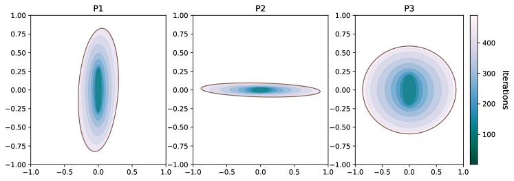
Figure 2: Noise accumulation over SAPD iterates: $\{\Sigma_{n}\}$ converges to an equilibrium covariance $\Sigma^{\infty}$ due to convergence in distribution $z_{n}\operatorname{\overset{\mathcal{D}}{\longrightarrow}}z^{\infty}$ derived in Thereom 11. By Corollary 2, convergence occurs at a linear rate which is plotted for the level sets $\{z\in\mathbb{R}^{2}:z^{\top}\Sigma_{n}z=1\}$ for $d=1$. The constants $({\color[rgb]{0,0,0}c},\mu_{x},\mu_{y},\delta)$ for each problem from left to right: P1: $(1,4.4,1.5,35)$ - P2: $(1,2,20,50)$ - P3: $({\color[rgb]{0,0,0}10^{-3}},0.205,0.307,5)$, where $K=c\in\mathbb{R}$.

4.2 Tightness analysis

We discuss in this section that the constants given in Theorem 4 are tight in the sense that under the CP parameterization given in (2.3), which corresponds to a particular solution of the matrix inequality in (2.2), the dependency of these constants to $\theta$ and $p$ cannot be improved when the number of iterations $n$ is sufficiently large. To this end, we consider quadratic problems subject to additive isotropic Gaussian noise for which we can do exact computations, i.e., both $\{\Delta_{k}^{x}\}$ and $\{\Delta_{k}^{y}\}$ are i.i.d zero-mean Gaussian random vector sequences with isotropic covariances, and these sequences are independent from each other as well.

In Section 4.1, under the isotropic Gaussian noise assumption, we show that the distribution $\pi_{n}$ of the iterates $z_{n}\operatorname{\triangleq}(x_{n},y_{n})$ converges to a Gaussian distribution $\pi_{\infty}$ with mean $\operatorname{z^{\star}}=(\operatorname{x^{\star}},\operatorname{y^{\star}})$ and a covariance matrix $\Sigma^{\star}$ for which we provide a formula in (4.4). If we let $z_{\infty}$ denote a random variable with the stationary distribution $\pi_{\infty}$, Theorem 4 implies that

$$Q_{p}(\|z_{\infty}-\operatorname{z^{\star}}\|^{2})=\limsup_{n\to\infty}Q_{p}(\|z_{n}-\operatorname{z^{\star}}\|^{2})=\mathcal{O}\Big{(}(1-\theta)\delta^{2}\Big{(}1+\log\Big{(}\frac{1}{1-p}\Big{)}\Big{)}\Big{)},$$ (4.6)

as $\theta\to 1$. This upper bound (grows) scales linearly with respect to $1-\theta$ and $\log(\frac{1}{1-p})$, and a natural question is whether this scaling can be improved. In the next proposition we provide lower bounds on the quantiles of $\|z_{\infty}\|^{2}$ that also grows linearly with respect to $1-\theta$ and $\log(\frac{1}{1-p})$, matching the upper bound in (4.6). Therefore, we conclude that our analysis is tight in the sense that we cannot expect to improve our bound in (4.6) in terms of its dependency to $p$ and $1-\theta$.

Theorem 12.

Let $(z_{n})_{n\geq 0}$ be the sequence initialized at an arbitrary tuple $z_{0}=(x_{0},y_{0})$ generated by SAPD under the parameterization (2.3) on the quadratic problem (4.1) where $\operatorname{z^{\star}}=(0,0)$. Then, the sequence $(z_{n})_{n\geq 0}$ converges in distribution to a Gaussian vector $z_{\infty}$. Furthermore, for any $p\in(0,1)$, $p$-th quantile $Q_{p}(\|z_{\infty}-\operatorname{z^{\star}}\|^{2})$ admits the bound

$$\psi_{1}(p,\theta)\leq Q_{p}(\|z_{\infty}-\operatorname{z^{\star}}\|^{2})\leq\psi_{2}(p,\theta),$$

where $\psi_{1}(p,\theta)=(1-\theta)\log(1/(1-p))\Theta(1)$ and $\psi_{2}(p,\theta)=(1-\theta)\mathcal{O}(1+\log(1/(1-p)))$, as $\theta\to 1$.

Proof.

The proof is provided in Section C.4 of the appendix. ∎

5 Proof of Main Results

5.1 Concentration inequalities through recursive control

This section presents general concentration inequalities that will be specialized later for the analysis of SAPD. The first result is a recursive concentration inequality extending the result provided in (Cutler et al., 2021, Proposition 6.7), which is used in the analysis of the stochastic gradient descent (SGD) method for minimization of a smooth strongly convex function in (Cutler et al., 2021). Our variant of this inequality enables us to analyze saddle point problems with acceleration, providing new insights on their robustness properties.

Proposition 13.

Let $(\operatorname{\mathcal{F}}_{n})_{n\geq 0}$ be a filtration on $(\Omega,\operatorname{\mathcal{F}},\mathbb{P})$. Let $(V_{n})_{n\geq 0}$, $(T_{n})_{n\geq 0}$, and $(R_{n})_{n\geq 0}$, be three scalar stochastic processes adapted to $(\mathcal{F}_{n})_{n\geq 0}$ with following properties: there exist $\sigma_{R},\sigma_{T}>0$ such that for all $n\geq 0$,

• $V_{n}$ is non-negative;

• $\mathbb{E}\left[e^{\lambda{\color[rgb]{0,0,0}T_{n+1}}}|\operatorname{\mathcal{F}}_{n}\right]\leq e^{\lambda^{2}\sigma_{T}^{2}V_{n}}$ for all $\lambda>0$, i.e., $T_{n+1}$ conditioned on $\operatorname{\mathcal{F}}_{n}$ is subGaussian;

• $\mathbb{E}\left[e^{\lambda{\color[rgb]{0,0,0}R_{n+1}}}|\operatorname{\mathcal{F}}_{n}\right]\leq e^{\lambda\sigma^{2}_{R}}$ for all $\lambda\in[0,1/\sigma_{R}^{2}]$, i.e., $R_{n+1}$ conditioned on $\operatorname{\mathcal{F}}_{n}$ is subExponential.

If there exists $\rho\in(0,1)$ such that

$$V_{n+1}{\color[rgb]{0,0,0}-T_{n+1}-R_{n+1}}\leq\rho\;V_{n},\quad\forall n\geq 0,$$ (5.1)

then for all $\lambda\in\Big{(}0,\min\{\frac{1}{2\sigma_{R}^{2}},\frac{1-\rho}{4\sigma_{T}^{2}}\}\Big{)}$, it holds that $\mathbb{E}\left[e^{\lambda V_{n+1}}\right]\leq e^{\lambda\sigma_{R}^{2}}\mathbb{E}\left[e^{\frac{\lambda(1+\rho)}{2}V_{n}}\right]$, for $n\geq 0$.

Proof.

Our proof follows closely the arguments of (Cutler et al., 2021, Proposition 6.7). The main difference is in the term $T_{n+1}$ which takes the specific form $T_{n+1}=G_{n+1}\sqrt{V_{n}}$ in (Cutler et al., 2021), where $G_{n+1}$ conditioned on $\mathcal{F}_{n}$ is assumed to be subGaussian. For any $\lambda\geq 0$, (5.1) together with Cauchy-Schwarz inequality implies that

$$\begin{split}\mathbb{E}\left[e^{\lambda V_{n+1}}|\operatorname{\mathcal{F}}_{n}\right]&\leq e^{\lambda\rho V_{n}}\mathbb{E}\left[e^{\lambda{\color[rgb]{0,0,0}(T_{n+1}+R_{n+1})}}|\operatorname{\mathcal{F}}_{n}\right]\leq e^{\lambda\rho V_{n}}\mathbb{E}\left[e^{2\lambda{\color[rgb]{0,0,0}T_{n+1}}}|\operatorname{\mathcal{F}}_{n}\right]^{1/2}\mathbb{E}\left[e^{2\lambda{\color[rgb]{0,0,0}R_{n+1}}}|\operatorname{\mathcal{F}}_{n}\right]^{1/2}.\\ \end{split}$$

Thus for $\lambda\in\Big{(}0,\frac{1}{2\sigma_{R}^{2}}\Big{]}$, we have $\mathbb{E}\left[e^{\lambda V_{n+1}}|\operatorname{\mathcal{F}}_{n}\right]\leq e^{\lambda\sigma_{R}^{2}}e^{\lambda(\rho+2\lambda\sigma_{T}^{2})V_{n}}$. Setting $0\leq\lambda\leq\min\left\{\frac{1}{2\sigma_{R}^{2}},\frac{1-\rho}{4\sigma_{T}^{2}}\right\}$ and taking the non-conditional expectation, we ensure that $\mathbb{E}\left[e^{\lambda V_{n+1}}\right]\leq e^{\lambda\sigma_{R}^{2}}\mathbb{E}\left[e^{\lambda\frac{1+\rho}{2}V_{n}}\right]$. This completes the proof. ∎

Unrolling the above recursive property on the moment generating function of $V_{n}$ provides us with high probability results on $(V_{n})_{n\geq 0}$, given in the next result.

Proposition 14.

Let $V_{n},T_{n},R_{n}$ be defined as in Proposition 13. Then, for all $n\geq 0$ and $\lambda\in\left[0,\min\left\{\frac{1-\rho}{4\sigma_{T}^{2}},\frac{1}{2\sigma_{R}^{2}}\right\}\right]$,

$$\mathbb{E}\left[e^{\lambda V_{n}}\right]\leq e^{\frac{2\lambda\sigma_{R}^{2}}{1-\rho}}\mathbb{E}\left[e^{\lambda\left(\frac{1+\rho}{2}\right)^{n}V_{0}}\right].$$ (5.2)

Furthermore, if $V_{0}=C_{0}$ is constant, then

$$\operatorname{\mathbb{P}}\left[V_{n}\leq\left(\frac{1+\rho}{2}\right)^{n}C_{0}+\frac{2\sigma_{R}^{2}}{1-\rho}\left(1+\max\left\{1,2\leavevmode\nobreak\ \frac{\sigma_{T}^{2}}{\sigma_{R}^{2}}\right\}\log\left(\frac{1}{1-p}\right)\right)\right]\geq p.$$ (5.3)

Alternatively, if $V_{0}$ can be expressed as $V_{0}=C_{0}+\mathcal{U}$ such that $C_{0}\geq 0$ is constant and $\mathcal{U}$ satisfies $\mathbb{E}\left[e^{\lambda\mathcal{U}}\right]\leq e^{\alpha\lambda+\beta\lambda^{2}}$, for all $\lambda\in{\color[rgb]{0,0,0}\left[0,\frac{1}{\bar{\alpha}}\right]}$, for some constants $\alpha,\bar{\alpha}>0$ and $\beta\geq 0$, then for any $p\in{\color[rgb]{0,0,0}[0},1)$ and $\lambda\in[0,\gamma]$ where $\gamma\operatorname{\triangleq}\frac{1-\rho}{\max\{\bar{\alpha},2\sigma_{R}^{2},4\sigma_{T}^{2}\}}$, we have

$$\mathbb{P}\left(V_{n}\leq\left(\frac{1+\rho}{2}\right)^{n}(C_{0}+\alpha)+{\color[rgb]{0,0,0}\left(\frac{1+\rho}{2}\right)^{2n}\lambda\beta}+\frac{2\sigma_{R}^{2}}{1-\rho}+{\color[rgb]{0,0,0}\frac{1}{\lambda}}\log\left(\frac{1}{1-p}\right)\right)\geq p.$$ (5.4)

Proof.

Let us first prove by induction on $n$ that for all $\lambda\in\left(0,\min\left\{\frac{1-\rho}{4\sigma_{T}^{2}},\frac{1}{2\sigma_{R}^{2}}\right\}\right)$,

$$\mathbb{E}\left[e^{\lambda V_{n}}\right]\leq\mathbb{E}\left[e^{\lambda\left(\frac{1+\rho}{2}\right)^{n}V_{0}+\lambda\sigma_{R}^{2}\sum_{k=0}^{n-1}\left(\frac{1+\rho}{2}\right)^{k}}\right].$$ (5.5)

For $n=0$, this property holds trivially with the convention $\Sigma_{k=0}^{n-1}=0$ when $n=0$. Assuming the inequality holds for some $n\geq 0$, next we show it also holds for $n+1$. According to Proposition 13,

$$\begin{split}\mathbb{E}\left[e^{\lambda V_{n+1}}\right]&\leq e^{\lambda\sigma_{R}^{2}}\mathbb{E}\left[e^{\lambda\frac{1+\rho}{2}V_{n}}\right]\\ &\leq e^{\lambda\sigma_{R}^{2}}\mathbb{E}\left[e^{\lambda\frac{1+\rho}{2}\left(\frac{1+\rho}{2}\right)^{n}V_{0}+\lambda\frac{1+\rho}{2}\sigma_{R}^{2}\sum_{k=0}^{n-1}\left(\frac{1+\rho}{2}\right)^{k}}\right]=\mathbb{E}\left[e^{\lambda\left(\frac{1+\rho}{2}\right)^{n+1}V_{0}+\lambda\sigma_{R}^{2}\sum_{k=0}^{n}\left(\frac{1+\rho}{2}\right)^{k}}\right],\end{split}$$

where the second inequality follows from the induction hypothesis since

$$0<\lambda(1+\rho)/2\leq\lambda\leq\min\left\{\frac{1-\rho}{4\sigma_{T}^{2}},\frac{1}{2\sigma_{R}^{2}}\right\},$$

and this completes the induction. Thus, (5.2) follows from using $\sum_{k=0}^{n-1}\Big{(}\frac{1+\rho}{2}\Big{)}^{k}\leq\frac{2}{1-\rho}$ within (5.5). The remaining statements follow from a Chernoff bound; indeed, if $V_{0}=C_{0}$ is constant, we obtain

$$\operatorname{\mathbb{P}}\left[V_{n}\geq\left(\frac{1+\rho}{2}\right)^{n}{\color[rgb]{0,0,0}C_{0}}+\frac{2\sigma_{R}^{2}}{1-\rho}+t\right]\leq e^{{\color[rgb]{0,0,0}-\lambda t}},$$

for $\lambda=\frac{1-\rho}{2\max\{\sigma_{R}^{2},2\sigma_{T}^{2}\}}$ and $t=\frac{1}{\lambda}{\color[rgb]{0,0,0}\log(\frac{1}{1-p})}$, which implies the desired result. Next, suppose $V_{0}=C_{0}+\mathcal{U}$ for some constant $C_{0}$ and $\mathcal{U}$ as in the hypothesis. First, observe that for $\lambda\in\left(0,\min\left\{\frac{1-\rho}{4\sigma_{T}^{2}},\frac{1}{2\sigma_{R}^{2}},\frac{1}{\bar{\alpha}}\right\}\right)$,

$$\begin{split}\mathbb{E}\left[e^{\lambda V_{n}}\right]&\leq e^{\frac{2\lambda\sigma_{R}^{2}}{1-\rho}}\mathbb{E}\left[e^{\lambda\left(\frac{1+\rho}{2}\right)^{n}(C_{0}+\mathcal{U})}\right]\leq e^{\lambda\left(\left(\frac{1+\rho}{2}\right)^{n}(C_{0}+\alpha)+\frac{2\sigma_{R}^{2}}{1-\rho}\right)+\lambda^{2}\left(\frac{1+\rho}{2}\right)^{2n}\beta}.\end{split}$$ (5.6)

Thus, for all $t\geq 0$,

$$\operatorname{\mathbb{P}}\left(V_{n}\geq\left(\frac{1+\rho}{2}\right)^{n}(C_{0}+\alpha)+\frac{2\sigma_{R}^{2}}{1-\rho}+t\right)\leq e^{\lambda^{2}\left(\frac{1+\rho}{2}\right)^{2n}\beta-\lambda t}.$$

Fixing an arbitrary non-negative $\lambda$ such that $\lambda\leq\frac{1-\rho}{\max\{\bar{\alpha},2\sigma_{R}^{2},4\sigma_{T}^{2}\}}$, we have $\exp(\lambda^{2}\left(\frac{1+\rho}{2}\right)^{{\color[rgb]{0,0,0}2}n}\beta-\lambda t)=1-p\iff t=\lambda(\frac{1+\rho}{2})^{2n}\beta+\frac{1}{\lambda}\log(1/(1-p))$, which proves (5.4). ∎

Based on Proposition 14, as a corollary, one can derive convergence rates for the CVaR and EVaR risk measures of the scalar process $(V_{n})_{n\geq 0}$.

Corollary 15.

Let $V_{n},T_{n},R_{n},\gamma$ be defined as in Proposition 14. Then, for any $p\in{\color[rgb]{0,0,0}[0},1)$ and $\lambda\in[0,\gamma]$,

$$\operatorname{CVaR}_{p}(V_{n}^{\frac{1}{2}})\leq\left(\frac{1+\rho}{2}\right)^{{\color[rgb]{0,0,0}\frac{n}{2}}}\sqrt{C_{0}+\alpha+{\color[rgb]{0,0,0}\lambda}\beta}+{\color[rgb]{0,0,0}\sqrt{\frac{2}{1-\rho}\sigma_{R}^{2}+\frac{1}{{\color[rgb]{0,0,0}\lambda}}\left(1+\log\left(\frac{1}{1-p}\right)\right)}}.$$ (5.7)

Proof.

Note that the first and second terms on the right-hand side of (5.4) satisfy

$$\left(\frac{1+\rho}{2}\right)^{n}(C_{0}+\alpha)+{\color[rgb]{0,0,0}\left(\frac{1+\rho}{2}\right)^{2n}\lambda\beta}\leq\left(\frac{1+\rho}{2}\right)^{n}(C_{0}+\alpha+\lambda\beta).$$

Hence, by integrating the resulting looser bound with respect to $p$, and using CVaR’s integral formulation in (2.9), we obtain

$$\operatorname{CVaR}_{p}(V_{n})\leq\left(\frac{1+\rho}{2}\right)^{n}\left(C_{0}+\alpha+{\lambda\beta}\right)+\frac{2\sigma_{R}^{2}}{1-\rho}+{\frac{1}{\lambda}}\left(1+\log\left(\frac{1}{1-p}\right)\right),$$

which directly implies (5.7), due to Lemma (21) and the sub-additivity of $t\mapsto\sqrt{t}$. ∎

Corollary 16.

Let $V_{n},T_{n},R_{n},\gamma$ be defined as in Proposition 14. Then, for any $p\in{\color[rgb]{0,0,0}[0},1)$, and $\lambda\in[0,\gamma]$,

$$\operatorname{EVaR}_{p}\left(V_{n}^{\frac{1}{2}}\right)\leq\left(\frac{1+\rho}{2}\right)^{n/2}{\color[rgb]{0,0,0}\sqrt{C_{0}+\alpha+{\color[rgb]{0,0,0}\lambda}\beta}}+\sqrt{\frac{2}{1-\rho}}\sigma_{R}+{\color[rgb]{0,0,0}\left(\sqrt{\frac{1}{{\color[rgb]{0,0,0}\lambda}}\log(\frac{1}{1-p})}+\frac{\sqrt{\pi}}{\sqrt{{\color[rgb]{0,0,0}\lambda}}}\right)}.$$ (5.8)

Proof.

The bound in (5.4) of Proposition 14 ensures that for all $p\in[0,1)$ and $\lambda\in[0,\gamma]$, the $p$-th quantile of $V_{n}$ satisfies

$$Q_{p}\left(V_{n}\right)\leq\left(\frac{1+\rho}{2}\right)^{n}\left(C_{0}+\alpha+{\color[rgb]{0,0,0}\lambda}\beta\right)+\frac{2\sigma_{R}^{2}}{1-\rho}+\frac{1}{{\color[rgb]{0,0,0}\lambda}}\log\left(\frac{1}{1-p}\right);$$

hence, non-negativity of $V_{n}$, Lemma 21 and sub-additivity of $t\mapsto\sqrt{t}$ together imply that

$$Q_{p}\left(V_{n}^{1/2}\right)\leq\left(\frac{1+\rho}{2}\right)^{n/2}{\color[rgb]{0,0,0}\sqrt{C_{0}+\alpha+\lambda\beta}}+\sqrt{\frac{2}{1-\rho}}\sigma_{R}+{\color[rgb]{0,0,0}\frac{1}{\sqrt{\lambda}}}\log\left(\frac{1}{1-p}\right)^{1/2}.$$ (5.9)

For $n\geq 0$, let $U_{n}\operatorname{\triangleq}V_{n}^{1/2}-\left(\frac{1+\rho}{2}\right)^{n/2}{\color[rgb]{0,0,0}\sqrt{C_{0}+\alpha+\lambda\beta}}-\sqrt{\frac{2}{1-\rho}}\sigma_{R},$ and note that (5.9) implies

$$\mathbb{P}\left(U_{n}>t\right)\leqslant e^{-{\color[rgb]{0,0,0}\lambda}t^{2}}\quad{\color[rgb]{0,0,0}\forall\leavevmode\nobreak\ t\geq 0.}$$ (5.10)

Therefore, following standard arguments from (Vershynin, 2018), we have for any $\eta>0$ that

$$\mathbb{E}(e^{{\color[rgb]{0,0,0}\eta}U_{n}}) = \int_{0}^{\infty}\operatorname{\mathbb{P}}\left[e^{{\color[rgb]{0,0,0}\eta}U_{n}}>t\right]dt=\int_{-\infty}^{\infty}\operatorname{\mathbb{P}}\left[e^{{\color[rgb]{0,0,0}\eta}U_{n}}>e^{u}\right]e^{u}du$$

$$= \int_{-\infty}^{0}\operatorname{\mathbb{P}}\left[e^{{\color[rgb]{0,0,0}\eta}U_{n}}>e^{u}\right]e^{u}du+\int_{0}^{\infty}\operatorname{\mathbb{P}}\left[e^{{\color[rgb]{0,0,0}\eta}U_{n}}>e^{u}\right]e^{u}du$$

$$\leq \int_{-\infty}^{0}e^{u}du+\int_{0}^{\infty}{\color[rgb]{0,0,0}e^{-\frac{\lambda}{\eta^{2}}u^{2}}}e^{u}du=1+{\color[rgb]{0,0,0}e^{\frac{\eta^{2}}{4\lambda}}}\int_{0}^{\infty}{\color[rgb]{0,0,0}e^{-\frac{\lambda}{\eta^{2}}(u-\frac{\eta^{2}}{2\lambda})^{2}}}du1+{\color[rgb]{0,0,0}e^{\frac{\eta^{2}}{4\lambda}}\int_{-\frac{\eta^{2}}{2\lambda}}^{\infty}e^{-\frac{\lambda}{\eta^{2}}s^{2}}ds}$$

$$\leq 1+{\color[rgb]{0,0,0}\eta e^{\frac{\eta^{2}}{4\lambda}}\sqrt{\frac{\pi}{\lambda}}}\leq{\color[rgb]{0,0,0}\Big{(}1+\eta\sqrt{\frac{\pi}{\lambda}}\Big{)}e^{\frac{\eta^{2}}{4\lambda}}},$$

where we used (5.10). On the other hand,

$$\operatorname{EVaR}_{p}\left[U_{n}\right] = \inf_{\eta>0}\Big{\{}-\eta^{-1}\log(1-p)+\eta^{-1}{\color[rgb]{0,0,0}\log}\operatorname{\mathbb{E}}\left[e^{\eta U_{n}}\right]\Big{\}}$$

$$\leq \inf_{\eta>0}-\eta^{-1}\log(1-p)+\eta^{-1}\left(\eta^{2}/(4\lambda)+\eta\sqrt{\pi}/\sqrt{\lambda}\right)=\sqrt{\log(\frac{1}{1-p})}/\sqrt{\lambda}+\sqrt{\pi}/\sqrt{\lambda},$$

where we used $\log(1+x)\leq x$ for $x\geq 0$. Finally, by translation invariance of the $\operatorname{EVaR}$, we obtain $\operatorname{EVaR}_{p}\left[V_{n}^{\frac{1}{2}}\right]\leq\left(\frac{1+\rho}{2}\right)^{n/2}{\color[rgb]{0,0,0}\sqrt{C_{0}+\alpha+\lambda\beta}}+\sqrt{\frac{2}{1-\rho}}\sigma_{R}+{\color[rgb]{0,0,0}\left(\sqrt{\frac{1}{\lambda}\log\Big{(}\frac{1}{1-p}\Big{)}}+\frac{\sqrt{\pi}}{\sqrt{\lambda}}\right)}$. ∎

We finish with a bound on the $\chi^{2}$-based risk measure, as defined in Table 2.3.

Corollary 17.

Let $V_{n},T_{n},R_{n},\gamma$ be defined as in Proposition 14. Then, for any $r>0$, and $\lambda\in[0,\gamma]$,

$$\operatorname{\mathcal{R}}_{\chi^{2},r}\left(V_{n}^{\frac{1}{2}}\right)\leq\left(\frac{1+\rho}{2}\right)^{n/2}\sqrt{C_{0}+\alpha+{\color[rgb]{0,0,0}\lambda}\beta}+\sqrt{\frac{2}{1-\rho}}\sigma_{R}+\left(\sqrt{\frac{1}{{\color[rgb]{0,0,0}\lambda}}\log\left(1+r\right)}+\frac{\sqrt{\pi}}{{\color[rgb]{0,0,0}\sqrt{\lambda}}}\right).$$ (5.11)

Proof.

By(Gibbs and Su, 2002, Theorem 5), for all ${\color[rgb]{0,0,0}\mathbb{Q}}\ll\operatorname{\mathbb{P}}$, we have $D_{\varphi_{\text{KL}}}(\mathbb{Q}{\color[rgb]{0,0,0}\|}\operatorname{\mathbb{P}})\leq\log\left(1+D_{\varphi_{\chi^{2}}}(\mathbb{Q}{\color[rgb]{0,0,0}\|}\operatorname{\mathbb{P}})\right)$, where $\varphi_{\text{KL}}(t)=t\log(t)-t+1$. Therefore, for any integrable random variable $U:\Omega\to\operatorname{\mathbb{R}}$,

$$\sup_{{\color[rgb]{0,0,0}\mathbb{Q}:}D_{\varphi_{\chi^{2}}}(\mathbb{Q}{\color[rgb]{0,0,0}\|}\operatorname{\mathbb{P}})\leq r}\operatorname{\mathbb{E}}_{\mathbb{Q}}[U]{\color[rgb]{0,0,0}\leq}\sup_{{\color[rgb]{0,0,0}\mathbb{Q}:}D_{\varphi_{\text{KL}}}(\mathbb{Q}{\color[rgb]{0,0,0}\|}\operatorname{\mathbb{P}})\leq\log(1+r)}\operatorname{\mathbb{E}}_{\mathbb{Q}}[U]=\operatorname{EVaR}_{1-1/(1+r)}(U),$$

whenever $\operatorname{EVaR}_{1-1/(1+r)}(U)<\infty$, where we used the EVaR representation given in Table 2.3. The statement follows directly from Corollary 16. ∎

In the next section, we design scalar processes $V_{n},T_{n},R_{n}$ which satisfy the above assumptions while dominating the error $\mathcal{D}_{n}$ on SAPD iterates, so that Proposition 13, Corollaries 16 and 17 will allow us to prove our main results, stated in Theorem 4 and Theorem 10.

5.2 Proofs of Theorem 4 and Theorem 10

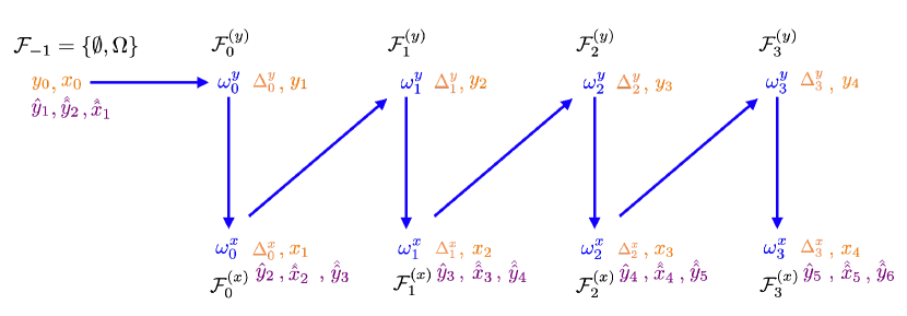
Figure 3: Measurability of SAPD sequences. Our analysis is made possible by the introduction of predictable counterparts $\operatorname{\hat{x}}_{k},\operatorname{\hat{\hat{x}}}_{k},\operatorname{\hat{y}}_{k},\operatorname{\hat{\hat{y}}}_{k}$ to the iterates $x_{k},y_{k}$ as defined in (5.12).

For proving the main results of this paper, namely Theorem 4 and Theorem 10, the application of the recursive control inequality from Section 5.1 is not straightforward. In particular, Gauss-Seidel type updates within SAPD significantly complicate the measurability properties of SAPD iterate sequence, as illustrated in Figure 3: the iterates $x_{k}$ and $y_{k}$ are measurable with respect to different filtrations $\mathcal{F}_{k-1}^{(x)}$ and $\mathcal{F}_{k-1}^{(y)}$. We circumvent this issue by introducing a stochastic process $\{V_{k}\}_{k\geq 0}$ that almost surely upper bounds the distance to the saddle point while exhibiting simpler measurability characteristics as discussed next. We note that even though algorithms with Gauss-Seidel type updates, such as SAPD, are significantly more complicated to analyze than their Jacobi counterparts, such an analysis is rewarding in the sense that algorithms with Gauss-Seidel type updates can often be faster than those using Jacobi type updates, see (Zhang et al., 2023, 2022). Indeed, our analysis for SAPD allowed us to obtain high-probability bounds that demonstrate an accelerated behavior for a stochastic primal-dual algorithm for SP problems.

5.2.1 Proof of Theorem 4

Our proof combines several ingredients. Let $(\tau,\sigma,\theta,\rho,{\color[rgb]{0,0,0}\alpha})$ be a solution to the matrix inequality in (2.2). Recall the weighted distance square metric $\mathcal{D}_{n}{=}\frac{1}{2\tau}\|x_{n}-\operatorname{x^{\star}}\|+\frac{1-\alpha\sigma}{2\sigma}\|y_{n}-\operatorname{y^{\star}}\|^{2}$ we introduced in (2.4). In the proof, we use a scaled version $\mathcal{E}_{n}\triangleq\mathcal{D}_{n}/\rho$ for $n\geq 0$ that simplifies the analysis. We first introduce the following auxiliary iterates $\operatorname{\hat{y}}_{k},\operatorname{\hat{\hat{x}}}_{k},\operatorname{\hat{\hat{y}}}_{k}$ which can be interpreted as the “noise-free counterparts" to the actual iterates $x_{k},y_{k}$ in the sense they represent roughly how the algorithm would behave if the gradients were deterministic in lieu of being stochastic at step $k$:

$$\operatorname{\hat{\hat{x}}}_{0}\operatorname{\triangleq}x_{0}, \operatorname{\hat{\hat{x}}}_{k+1}\operatorname{\triangleq}\text{prox}_{\tau f}\left(x_{k}-\tau\operatorname{\nabla_{x}\operatorname{\Phi}}(x_{k},\operatorname{\hat{y}}_{k+1})\right),$$ (5.12)

$$\operatorname{\hat{y}}_{0}\operatorname{\triangleq}\operatorname{\hat{\hat{y}}}_{0}\operatorname{\triangleq}y_{0}, \operatorname{\hat{y}}_{k+1}\operatorname{\triangleq}\text{prox}_{\sigma g}\Big{(}y_{k}+\sigma(1+\theta)\operatorname{\nabla_{y}\operatorname{\Phi}}(x_{k},y_{k})-{\color[rgb]{0,0,0}\sigma}\theta\operatorname{\nabla_{y}\operatorname{\Phi}}(x_{k-1},y_{k-1})\Big{)},$$ (5.13)

$$\operatorname{\hat{\hat{y}}}_{k+1}\operatorname{\triangleq}\text{prox}_{\sigma g}\left(\operatorname{\hat{y}}_{k}+\sigma(1+\theta)\operatorname{\nabla_{y}\operatorname{\Phi}}(\operatorname{\hat{\hat{x}}}_{k},\operatorname{\hat{y}}_{k})-\sigma\theta\operatorname{\nabla_{y}\operatorname{\Phi}}(x_{k-1},y_{k-1})\right).$$ (5.14)

where we recall that $x_{-1}=x_{0}$ and $y_{-1}=y_{0}$ (see Algorithm 1). These auxiliary iterates whose measurability properties are illustrated in Figure 3, will be key for being able to apply Proposition 14 to obtain high-probability results for SAPD. Our proof is based on establishing an almost sure upper bound of the quantity $\mathcal{E}_{n+1}+\mathcal{E}_{n}$ by a scalar process $V_{n}$, and then showing that our choice of $V_{n}$ satisfies the assumptions of Proposition 13. This will then directly yield the desired high-probability estimates for SAPD. We start with a proposition that provides an almost sure bound to the scaled squared distance metric $\mathcal{E}_{n}$. Although this bound is already present in substance in (Zhang et al., 2023), it does not appear explicitly. For completeness, in Appendix B.1, we provide its proof based on various arguments developed in (Zhang et al., 2023).

Proposition 18.

Let $(x_{n},y_{n})$ be the sequence generated by SAPD, intialized at an arbitrary tuple ${(x_{-1},y_{-1})}=(x_{0},y_{0})\in\operatorname{\mathcal{X}}\times\operatorname{\mathcal{Y}}$. Provided that there exists $\tau,\sigma>0$, and $\theta\geq 0$ that satisfy (2.2) for some $\rho\in(0,1)$ and $\alpha\in{[0,\sigma^{-1})}$, the following almost sure bound on $\mathcal{E}_{n}$,

$$\mathcal{E}_{n}\leq\rho^{n-1}\mathcal{D}_{\tau,\sigma}+\sum_{k=0}^{n-1}\rho^{n-1-k}\Big{(}\langle\Delta_{k}^{x},\operatorname{x^{\star}}-x_{k+1}\rangle+\langle(1+\theta)\Delta_{k}^{y}-\theta\Delta_{k-1}^{y},y_{k+1}-\operatorname{y^{\star}}\rangle\Big{)},$$ (5.15)

holds for all $n\geq 1$, where $\mathcal{E}_{n}{\color[rgb]{0,0,0}=}\frac{1}{2\rho\tau}\|x_{n}-\operatorname{x^{\star}}\|^{2}+\frac{1-\alpha\sigma}{2\rho\sigma}\|y_{n}-\operatorname{y^{\star}}\|^{2}$, and $\mathcal{D}_{\tau,\sigma}{\color[rgb]{0,0,0}=}\frac{1}{2\tau}\|x_{0}-\operatorname{x^{\star}}\|^{2}+\frac{1}{2\sigma}\|y_{0}-\operatorname{y^{\star}}\|^{2}$.

Proof.

The proof is provided in Appendix B.1. ∎

Now, equipped with Proposition 18, we can write

$$\begin{split}\mathcal{E}_{n}&\leq\rho^{n-1}\mathcal{D}_{\tau,\sigma}+\sum_{k=0}^{n-1}\rho^{n-1-k}\Big{(}\langle\Delta_{k}^{x},\operatorname{x^{\star}}-x_{k+1}\rangle+\langle(1+\theta)\Delta_{k}^{y}-\theta\Delta_{k-1}^{y},y_{k+1}-\operatorname{y^{\star}}\rangle\Big{)}\\ &=\rho^{n-1}\mathcal{D}_{\tau,\sigma}\begin{aligned} &+\sum_{k=0}^{n-1}\rho^{n-1-k}\left(\langle\Delta_{k}^{x},\operatorname{x^{\star}}-\operatorname{\hat{\hat{x}}}_{k+1}\rangle+(1+\theta)\langle\Delta_{k}^{y},\operatorname{\hat{y}}_{k+1}-\operatorname{y^{\star}}\rangle-\theta\langle\Delta_{k-1}^{y},\operatorname{\hat{\hat{y}}}_{k+1}-\operatorname{y^{\star}}\rangle\right)\\ &+\sum_{k=0}^{n-1}\rho^{n-1-k}\left(\langle\Delta_{k}^{x},\operatorname{\hat{\hat{x}}}_{k+1}-x_{k+1}\rangle+(1+\theta)\langle\Delta_{k}^{y},y_{k+1}-\operatorname{\hat{y}}_{k+1}\rangle-\theta\langle\Delta_{k-1}^{y},y_{k+1}-\operatorname{\hat{\hat{y}}}_{k+1}\rangle\right).\\ \end{aligned}\end{split}$$ (5.16)

For $k\geq 0$, introducing the scalar quantities

$${P}_{k}^{(1)}\operatorname{\triangleq}\langle\Delta_{k}^{x},\operatorname{x^{\star}}-\operatorname{\hat{\hat{x}}}_{k+1}\rangle+(1+\theta)\langle\Delta_{k}^{y},\operatorname{\hat{y}}_{k+1}-\operatorname{y^{\star}}\rangle,\qquad{P}_{k}^{(2)}\operatorname{\triangleq}\frac{-\theta}{\rho}\langle\Delta_{k}^{y},\operatorname{\hat{\hat{y}}}_{k+2}-\operatorname{y^{\star}}\rangle,$$ (5.17a)

$$Q_{k}\operatorname{\triangleq}\langle\Delta_{k}^{x},\operatorname{\hat{\hat{x}}}_{k+1}-x_{k+1}\rangle+(1+\theta)\langle\Delta_{k}^{y},y_{k+1}-\operatorname{\hat{y}}_{k+1}\rangle-\theta\langle\Delta_{k-1}^{y},y_{k+1}-\operatorname{\hat{\hat{y}}}_{k+1}\rangle,$$ (5.17b)

rearranging the sums in (5.16) and using $\Delta_{-1}^{y}=\mathbf{0}$, we may write (5.16) equivalently as follows:

$$\mathcal{E}_{n}\leq\rho^{n-1}\mathcal{D}_{\tau,\sigma}+\sum_{k=0}^{n-1}\rho^{n-1-k}{P}_{k}^{(1)}+\sum_{k={\color[rgb]{0,0,0}0}}^{n-2}\rho^{n-1-k}{P}_{k}^{(2)}+\sum_{k=0}^{n-1}\rho^{n-1-k}Q_{k}.$$

Now notice that for $n\geq 0$,

$$\begin{split}\mathcal{E}_{n+1}&+\mathcal{E}_{n}\leq\begin{aligned} \left(1+\frac{1}{\rho}\right)&\left(\rho^{n}\mathcal{D}_{\tau,\sigma}+\sum_{k=0}^{n-1}\rho^{n-k}{P}_{k}^{(1)}+\sum_{k=0}^{n-2}\rho^{n-k}{P}_{k}^{(2)}+\sum_{k=0}^{n-1}\rho^{n-k}Q_{k}\right)+{P}_{n}^{(1)}+\rho{P}_{n-1}^{(2)}+Q_{n}\\ \end{aligned}\\ &\qquad\leavevmode\nobreak\ ={\begin{aligned} \left(1+\frac{1}{\rho}\right)&\left(\rho^{n}\mathcal{D}_{\tau,\sigma}+\sum_{k=0}^{n}\rho^{n-k}{P}_{k}^{(1)}+\sum_{k=0}^{n}\rho^{n-k}{P}_{k}^{(2)}\right)\\ &+\left(1+\frac{1}{\rho}\right)\left(\frac{-1}{1+\rho}{P}_{n}^{(1)}-{P}_{n}^{(2)}-\frac{\rho}{1+\rho}{P}_{n-1}^{(2)}{-\frac{1}{1+\rho}Q_{n}+\sum_{k=0}^{n}\rho^{n-k}Q_{k}}\right).\\ \end{aligned}}\\ \end{split}$$ (5.18)

We next present a lemma which bounds the terms on the right-hand side of the above equality.

Lemma 19.

Let ${P}_{n}^{(1)},{P}_{n}^{(2)}$ and $Q_{n}$ be defined as in (5.17). Then, for any $n\geq{\color[rgb]{0,0,0}0}$,

$$\begin{split}{\frac{-1}{1+\rho}{P}_{n}^{(1)}-{P}_{n}^{(2)}-\frac{\rho}{1+\rho}{P}_{n-1}^{(2)}}&{-\frac{1}{1+\rho}Q_{n}+\sum_{k=0}^{n}\rho^{n-k}Q_{k}}\\ &\leq{\frac{\rho}{2(1+\rho)}(\mathcal{E}_{n+1}+\mathcal{E}_{n})+\sum_{k=0}^{n}\rho^{n-k}\left(\mathcal{Q}_{x}\|\Delta_{k}^{x}\|^{2}+\mathcal{Q}_{y}\|\Delta_{k}^{y}\|^{2}\right)},\end{split}$$

for some positive constants $\mathcal{Q}_{x}$ and $\mathcal{Q}_{y}$, which depend only on the algorithm and problem parameters, and are provided explicitly in Table 2 of Appendix D.

Proof.

The proof is provided in Appendix B.2.1. ∎

Applying Lemma 19 to the inequality (5.18), we obtain

$${\frac{\rho}{2(1+\rho)}\left(\mathcal{E}_{n+1}+\mathcal{E}_{n}\right)}\leq\rho^{n}\mathcal{D}_{\tau,\sigma}$$ (5.19)

For $n\in\operatorname{\mathbb{N}}$, we define $V_{n}$, $T_{n+1}$ and $R_{n+1}$ as follows:

$$\begin{split}V_{n}&\operatorname{\triangleq}\rho^{n}\mathcal{D}_{\tau,\sigma}+\sum_{k=0}^{n}\rho^{n-k}\Big{(}{P}_{k}^{(1)}+{P}_{k}^{(2)}\Big{)}+\sum_{k=0}^{n}\rho^{n-k}\Big{(}\mathcal{Q}_{x}\|\Delta_{k}^{x}\|^{2}+\mathcal{Q}_{y}\|\Delta_{k}^{y}\|^{2}\Big{)},\\ {\color[rgb]{0,0,0}T_{n+1}}&\operatorname{\triangleq}{P}_{n+1}^{(1)}+{P}_{n+1}^{(2)},\qquad{\color[rgb]{0,0,0}R_{n+1}}\operatorname{\triangleq}{\;\mathcal{Q}_{x}\|\Delta_{n+1}^{x}\|^{2}+\mathcal{Q}_{y}\|\Delta_{n+1}^{y}\|^{2}};\\ \end{split}$$ (5.20)

therefore, (5.19) implies that

$${\frac{\rho}{2(1+\rho)}\left(\mathcal{E}_{n+1}+\mathcal{E}_{n}\right)}\leq V_{n},\quad\forall\leavevmode\nobreak\ n\geq 0,\quad\text{a.s.}$$ (5.21)

Next, we argue that $V_{n}$ satisfies the assumptions of the recursive control inequality in (13). To achieve this goal, we will use the following lemma.

Lemma 20.

For any $k\in\operatorname{\mathbb{N}}$ and $\rho\in(0,1)$, the following inequalities,

$$\begin{split}8\|\operatorname{\hat{\hat{x}}}_{k+1}-\operatorname{x^{\star}}\|^{2}&\leq\|A_{1}\|^{2}\;\frac{\rho}{2(1+\rho)}\left(\mathcal{E}_{k}+\mathcal{E}_{k-1}\right),\\ 16{(1+\theta)^{2}}\|\operatorname{\hat{y}}_{k+1}-\operatorname{y^{\star}}\|^{2}&\leq\|A_{2}\|^{2}\;\frac{\rho}{2(1+\rho)}\left(\mathcal{E}_{k}+\mathcal{E}_{k-1}\right),\\ 16{\frac{\theta^{2}}{\rho^{2}}}\|\operatorname{\hat{\hat{y}}}_{k+2}-\operatorname{y^{\star}}\|^{2}&\leq\|A_{3}\|^{2}\;\frac{\rho}{2(1+\rho)}\left(\mathcal{E}_{k}+\mathcal{E}_{k-1}\right),\\ \end{split}$$ (5.22)

hold almost surely with the convention that $\mathcal{E}_{-1}\triangleq\mathcal{E}_{0}$, for some vectors $A_{1},A_{2},A_{3}\in\mathbb{R}^{4}$ which are explicitly provided in Table 3 of Appendix D.

Proof.

The proof is provided in Appendix B.2.2. ∎

Let us now show that $V_{n}$ satisfies the assumptions of the recursive control inequality in (13). Indeed, for any $n\geq 0$, $V_{n+1}-V_{n}={\color[rgb]{0,0,0}(\rho-1)V_{n}}+{P}_{n+1}^{(1)}+{P}_{n+1}^{(2)}+{\mathcal{Q}_{x}\|\Delta_{n+1}^{x}\|^{2}+\mathcal{Q}_{y}\|\Delta_{n+1}^{y}\|^{2}}$, which is equivalent to $V_{n+1}{=}\rho V_{n}{\color[rgb]{0,0,0}+T_{n+1}+R_{n+1}}$. Let $\left(\operatorname{\mathcal{F}}_{n}\right)_{n\geq{\color[rgb]{0,0,0}-1}}$ be the filtration defined as $\operatorname{\mathcal{F}}_{-1}\operatorname{\triangleq}\{\emptyset,\Omega\}$, and $\operatorname{\mathcal{F}}_{n}\triangleq{\operatorname{\mathcal{F}}_{n}^{x}}=\sigma\left(\operatorname{\mathcal{F}}_{n-1}\cup\;\sigma(\Delta_{n}^{y})\cup\sigma(\Delta_{n}^{x})\right)$, for all $n\geq 0$. We first observe that for all $n\in\operatorname{\mathbb{N}}$, $V_{n}$, $T_{n}$ and $R_{n}$ are $\operatorname{\mathcal{F}}_{n}$-measurable; moreover, $V_{n}$ is non-negative due to (5.21). Second, for any $n\geq 0$, since $\Delta_{n}^{x}$ and $\Delta_{n}^{y}$ are norm-subGaussian conditioned respectively on $\operatorname{\mathcal{F}}_{n}^{y}$ and $\operatorname{\mathcal{F}}_{n-1}^{x}$, for any $\lambda\geq 0$, we get that

$$\begin{split}\mathbb{E}\left[e^{\lambda{\color[rgb]{0,0,0}T_{n+1}}}|\operatorname{\mathcal{F}}_{n}\right]&={\mathbb{E}\Bigg{[}e^{\lambda\Big{\langle}\Delta_{n+1}^{y},\leavevmode\nobreak\ (1+\theta)\left(\operatorname{\hat{y}}_{n+2}-\operatorname{y^{\star}}\right)-\theta\rho^{-1}(\operatorname{\hat{\hat{y}}}_{n+3}-\operatorname{y^{\star}})\Big{\rangle}}\operatorname{\mathbb{E}}\Bigg{[}e^{\lambda\langle\Delta_{n+1}^{x},\operatorname{x^{\star}}-\operatorname{\hat{\hat{x}}}_{n+2}\rangle}\Big{|}\operatorname{\mathcal{F}}_{n+1}^{y}\Bigg{]}\Big{|}\operatorname{\mathcal{F}}_{n}\Bigg{]}}\\ &\leq{e^{8\lambda^{2}\left(\|\operatorname{\hat{\hat{x}}}_{n+2}-\operatorname{x^{\star}}\|^{2}\delta_{x}^{2}+\|(1+\theta)\left(\operatorname{\hat{y}}_{n+2}-\operatorname{y^{\star}}\right)-\theta\rho^{-1}\left(\operatorname{\hat{\hat{y}}}_{n+3}-\operatorname{y^{\star}}\right)\|^{2}\delta_{y}^{2}\right)}}\\ &\leq{e^{8\lambda^{2}\left(\|\operatorname{\hat{\hat{x}}}_{n+2}-\operatorname{x^{\star}}\|^{2}\delta_{x}^{2}+2(1+\theta)^{2}\|\operatorname{\hat{y}}_{n+2}-\operatorname{y^{\star}}\|^{2}+2\theta^{{2}}\rho^{-{2}}\|\operatorname{\hat{\hat{y}}}_{n+3}-\operatorname{y^{\star}}\|^{2}\delta_{y}^{2}\right)}},\\ \end{split}$$

where we used Lemma 3 and the inequality $(a+b)^{2}\leq 2a^{2}+2b^{2}$ for scalars $a,b$ in the last step, noting that $\operatorname{\hat{\hat{x}}}_{n+2}$, $\operatorname{\hat{y}}_{n+2}$, $\operatorname{\hat{\hat{y}}}_{n+3}$ are all $\mathcal{F}_{n}$-measurable. Hence, in view of Lemma 20 provided above and the bound in (5.21), we have

$${\mathbb{E}\left[e^{\lambda{\color[rgb]{0,0,0}T_{n+1}}}|\operatorname{\mathcal{F}}_{n}\right]\leq{e^{\lambda^{2}\left(\|A_{1}\|^{2}\delta_{x}^{2}+\left(\|A_{2}\|^{2}+\|A_{3}\|^{2}\right)\delta_{y}^{2}\right)\frac{\rho}{2(1+\rho)}(\mathcal{E}_{n+1}+\mathcal{E}_{n})}}\leq{e^{\lambda^{2}\Big{(}\|A_{1}\|^{2}\delta_{x}^{2}+\left(\|A_{2}\|^{2}+\|A_{3}\|^{2}\right)\delta_{y}^{2}\Big{)}V_{n}},}}$$ (5.23)

where we used (5.21) to obtain the second inequality. Third, for all $n\geq 0$ and $\lambda\in\left(0,{\frac{1}{4\max\{\mathcal{Q}_{x}\delta_{x}^{2},\mathcal{Q}_{y}\delta_{y}^{2}\}}}\right)$, we have in view of Lemma 2

$$\begin{split}\mathbb{E}\left[e^{\lambda{\color[rgb]{0,0,0}R_{n+1}}}|\operatorname{\mathcal{F}}_{n}\right]&={\operatorname{\mathbb{E}}\left[e^{\lambda\mathcal{Q}_{y}\|\Delta_{n+1}^{y}\|^{2}}\operatorname{\mathbb{E}}\left[e^{\lambda\mathcal{Q}_{x}\|{\color[rgb]{0,0,0}\Delta_{n+1}^{x}}\|^{2}}|\operatorname{\mathcal{F}}_{n+1}^{y}\right]|\operatorname{\mathcal{F}}_{n}\right]}\leq{\exp\left(8\lambda\left(\mathcal{Q}_{x}\delta_{x}^{2}+\mathcal{Q}_{y}\delta_{y}^{2}\right)\right).}\\ \end{split}$$ (5.24)

Finally, we next argue that $V_{0}$ can be expressed as $V_{0}=\mathcal{D}_{\tau,\sigma}+\mathcal{U}$ for some $\mathcal{U}$ satisfying $\mathbb{E}\left[e^{\lambda\mathcal{U}}\right]\leq e^{\alpha\lambda+\beta\lambda^{2}},\quad\forall\lambda\in{\color[rgb]{0,0,0}\left[0,\frac{1}{\bar{\alpha}}\right]}$, for some constants $\alpha,\bar{\alpha}>0$ and $\beta\geq 0$. First, note that $\operatorname{\hat{y}}_{1},\operatorname{\hat{\hat{x}}}{{}_{1}}$ and $\operatorname{\hat{\hat{y}}}_{2}$ are all deterministic quantities as they depend only on the initialization; hence, using the inequality $u^{\top}v\leq\frac{{\color[rgb]{0,0,0}\gamma}}{2(1-\rho)}\|u\|^{2}+\frac{(1-\rho)}{2{\color[rgb]{0,0,0}\gamma}}\|v\|^{2}$ for any $\gamma>0$, we observe that for all $\lambda\in\left[0,{\Big{(}4\max\{\left(\frac{1-\rho}{2{\mu_{x}}}+\mathcal{Q}_{x}\right)\delta_{x}^{2},\left({\frac{(1-\rho)}{{\mu_{y}}}}+\mathcal{Q}_{y}\right)\delta_{y}^{2}\}\Big{)}^{-1}}\right]$, we have

$$\begin{split}&\mathbb{E}\left[e^{\lambda(V_{0}-\mathcal{D}_{\tau,\sigma})}\right]=\mathbb{E}\left[e^{\lambda{\color[rgb]{0,0,0}\left({P}_{0}^{(1)}+{P}_{0}^{(2)}+{\mathcal{Q}_{x}\|\Delta_{0}^{x}\|^{2}+\mathcal{Q}_{y}\|\Delta_{0}^{y}\|^{2}}\right)}}\right]\\ &=\begin{aligned} t]{1}&\operatorname{\mathbb{E}}\left[e^{\lambda\langle\Delta_{0}^{x},\operatorname{x^{\star}}-\operatorname{\hat{\hat{x}}}_{1}\rangle+\lambda\langle\Delta_{0}^{y},(1+\theta)(\operatorname{\hat{y}}_{1}-\operatorname{y^{\star}})-\frac{\theta}{\rho}(\operatorname{\hat{\hat{y}}}_{2}-\operatorname{y^{\star}})\rangle{+\lambda\mathcal{Q}_{x}\|\Delta_{0}^{x}\|^{2}+\lambda\mathcal{Q}_{y}\|\Delta_{0}^{y}\|^{2}}}\right]\\ \end{aligned}\\ &\leq{\operatorname{\mathbb{E}}\begin{aligned} t]{1}&\left[e^{\frac{\lambda}{2(1-\rho)}\left({\color[rgb]{0,0,0}\mu_{x}}\|\operatorname{\hat{\hat{x}}}_{1}-\operatorname{x^{\star}}\|^{2}+(1+\theta)^{{\color[rgb]{0,0,0}2}}{\color[rgb]{0,0,0}\mu_{y}}\|\operatorname{\hat{y}}_{1}-\operatorname{y^{\star}}\|^{2}+\theta^{{\color[rgb]{0,0,0}2}}\rho^{-{\color[rgb]{0,0,0}2}}{\color[rgb]{0,0,0}\mu_{y}}\|\operatorname{\hat{\hat{y}}}_{2}-\operatorname{y^{\star}}\|^{2}\right)}\right.\\ &\left.e^{\frac{\lambda(1-\rho)}{2}\left({\color[rgb]{0,0,0}\frac{1}{\mu_{x}}}\|\Delta_{0}^{x}\|^{2}+{\color[rgb]{0,0,0}\frac{1}{\mu_{y}}}{\color[rgb]{0,0,0}\|\Delta_{0}^{y}\|^{2}}+{\color[rgb]{0,0,0}\frac{1}{\mu_{y}}}{\color[rgb]{0,0,0}\|\Delta_{0}^{y}\|^{2}}\right)+\lambda\mathcal{Q}_{x}\|\Delta_{0}^{x}\|^{2}+\lambda\mathcal{Q}_{y}\|\Delta_{0}^{y}\|^{2}}\right]\\ \end{aligned}}\\ &={\begin{aligned} t]{1}&e^{\frac{\lambda}{2(1-\rho)}\left({\color[rgb]{0,0,0}\mu_{x}}\|\operatorname{\hat{\hat{x}}}_{1}-\operatorname{x^{\star}}\|^{2}+(1+\theta)^{{\color[rgb]{0,0,0}2}}{\color[rgb]{0,0,0}\mu_{y}}\|\operatorname{\hat{y}}_{1}-\operatorname{y^{\star}}\|^{2}+\theta^{{\color[rgb]{0,0,0}2}}\rho^{-{\color[rgb]{0,0,0}2}}{\color[rgb]{0,0,0}\mu_{y}}\|\operatorname{\hat{\hat{y}}}_{2}-\operatorname{y^{\star}}\|^{2}\right)}\operatorname{\mathbb{E}}\left[e^{\lambda\left(\left(\frac{1-\rho}{2{\color[rgb]{0,0,0}\mu_{x}}}+\mathcal{Q}_{x}\right)\|\Delta_{0}^{x}\|^{2}+\left({\color[rgb]{0,0,0}\frac{1-\rho}{\mu_{y}}}+\mathcal{Q}_{y}\right)\|\Delta_{0}^{y}\|^{2}\right)}\right]\\ \end{aligned}}\\ \end{split}$$

Thus,

$$\begin{split}&\mathbb{E}\left[e^{\lambda(V_{0}-\mathcal{D}_{\tau,\sigma})}\right]\\ &\leq{e^{\frac{\lambda}{2(1-\rho)}\left({\color[rgb]{0,0,0}\mu_{x}}\|\operatorname{\hat{\hat{x}}}_{1}-\operatorname{x^{\star}}\|^{2}+(1+\theta)^{{\color[rgb]{0,0,0}2}}{\color[rgb]{0,0,0}\mu_{y}}\|\operatorname{\hat{y}}_{1}-\operatorname{y^{\star}}\|^{2}+\theta^{{\color[rgb]{0,0,0}2}}\rho^{-{\color[rgb]{0,0,0}2}}{\color[rgb]{0,0,0}\mu_{y}}\|\operatorname{\hat{\hat{y}}}_{2}-\operatorname{y^{\star}}\|^{2}\right)}e^{8\lambda\left(\left(\frac{1-\rho}{2{\color[rgb]{0,0,0}\mu_{x}}}+\mathcal{Q}_{x}\right)\delta_{x}^{2}+\left({\color[rgb]{0,0,0}\frac{1-\rho}{{\color[rgb]{0,0,0}\mu_{y}}}}+\mathcal{Q}_{y}\right)\delta_{y}^{2}\right)}}\\ &\leq{e^{\frac{\lambda}{2(1-\rho)}\left({\color[rgb]{0,0,0}\frac{\mu_{x}}{8}}\|A_{1}\|^{2}+{\color[rgb]{0,0,0}\frac{\mu_{y}}{16}}(\|A_{2}\|^{2}+\|A_{3}\|^{2})\right)\;{\color[rgb]{0,0,0}\frac{\rho}{2(1+\rho)}\;\frac{2}{\rho}}\mathcal{D}_{\tau,\sigma}}e^{8\lambda\left(\left(\frac{1-\rho}{2{\color[rgb]{0,0,0}\mu_{x}}}+\mathcal{Q}_{x}\right)\delta_{x}^{2}+\left({\color[rgb]{0,0,0}\frac{1-\rho}{{\color[rgb]{0,0,0}\mu_{y}}}}+\mathcal{Q}_{y}\right)\delta_{y}^{2}\right)}}\\ &\leq{e^{\frac{\lambda}{2(1-\rho)}\left({\color[rgb]{0,0,0}\frac{\mu_{x}}{8}}\|A_{1}\|^{2}+{\color[rgb]{0,0,0}\frac{\mu_{y}}{16}}(\|A_{2}\|^{2}+\|A_{3}\|^{2})\right)\mathcal{D}_{\tau,\sigma}}e^{8\lambda\left(\left(\frac{1-\rho}{2{\color[rgb]{0,0,0}\mu_{x}}}+\mathcal{Q}_{x}\right)\delta_{x}^{2}+\left({\color[rgb]{0,0,0}\frac{1-\rho}{{\color[rgb]{0,0,0}\mu_{y}}}}+\mathcal{Q}_{y}\right)\delta_{y}^{2}\right)}},\\ \end{split}$$

where the first inequality follows from Lemma 2, in the second inequality we used Lemma 20 given above, and the relation $\mathcal{E}_{0}+\mathcal{E}_{-1}=2\mathcal{E}_{0}{=}2\mathcal{D}_{0}/\rho\leq 2\mathcal{D}_{\tau,\sigma}/\rho$, which follows from $1-\alpha\sigma<1$ and the relations $x_{0}=x_{-1}$, $y_{0}=y_{-1}$. Hence, we can apply Proposition 14 to the $V_{n},R_{n},T_{n}$ sequence defined in (5.20) with the following choice of parameter values,

$$\begin{split}C_{0}&=\mathcal{D}_{\tau,\sigma},\quad\mathcal{U}={P}_{0}^{(1)}+{P}_{0}^{(2)}+\mathcal{Q}_{x}\|\Delta_{0}^{x}\|^{2}+\mathcal{Q}_{y}\|\Delta_{0}^{y}\|^{2},\\ \sigma_{T}^{2}&={\|A_{1}\|^{2}\delta_{x}^{2}+\left(\|A_{2}\|^{2}+\|A_{3}\|^{2}\right)\delta_{y}^{2}},\quad\sigma_{R}^{2}={8}\;(\mathcal{Q}_{x}\delta_{x}^{2}+\mathcal{Q}_{y}\delta_{y}^{2}),\\ \alpha&=\begin{aligned} \frac{1}{16(1-\rho)}\bigg{(}\mu_{x}\|A_{1}\|^{2}&+\frac{\mu_{y}}{2}(\|A_{2}\|^{2}+\|A_{3}\|^{2})\bigg{)}\;\mathcal{D}_{\tau,\sigma}\\ &+\left(4\frac{(1-\rho)}{\mu_{x}}+8\mathcal{Q}_{x}\right)\delta_{x}^{2}+\left({\color[rgb]{0,0,0}8\frac{(1-\rho)}{\mu_{y}}}+8\mathcal{Q}_{y}\right)\delta_{y}^{2},\end{aligned}\\ \bar{\alpha}&={4\max\left(\left(\frac{1-\rho}{2{\color[rgb]{0,0,0}\mu_{x}}}+\mathcal{Q}_{x}\right)\delta_{x}^{2},\left({\color[rgb]{0,0,0}\frac{(1-\rho)}{{\color[rgb]{0,0,0}\mu_{y}}}+\mathcal{Q}_{y}}\right)\delta_{y}^{2}\right)},\quad\beta=0,\end{split}$$ (5.25)

where $\mathcal{D}_{\tau,\sigma}$ is defined in the statement of Theorem 4. When we invoke Proposition 14, we set $\lambda=\tilde{\gamma}$ within (5.4) for some particular $\tilde{\gamma}>0$ such that $\tilde{\gamma}\leq\gamma$ as required by the proposition. Thus, for any $p\in(0,1)$ and $n\geq 0$, the following inequality

$$\begin{split}V_{n}\leq&\left(\frac{1+\rho}{2}\right)^{n}\bigg{(}\left(1+\frac{1}{{\color[rgb]{0,0,0}16}(1-\rho)}\left({\color[rgb]{0,0,0}\mu_{x}}\|A_{1}\|^{2}+{\color[rgb]{0,0,0}\frac{\mu_{y}}{2}}(\|A_{2}\|^{2}+\|A_{3}\|^{2})\right)\right)\mathcal{D}_{\tau,\sigma}\\ &\quad+\left(\frac{{\color[rgb]{0,0,0}4}(1-\rho)}{{\color[rgb]{0,0,0}\mu_{x}}}+{\color[rgb]{0,0,0}8}\mathcal{Q}_{x}\right)\delta_{x}^{2}+\left({\color[rgb]{0,0,0}8}\frac{(1-\rho)}{{\color[rgb]{0,0,0}\mu_{y}}}{\color[rgb]{0,0,0}+8\mathcal{Q}_{y}}\right)\delta_{y}^{2}\bigg{)}\\ &+\frac{{\color[rgb]{0,0,0}16}}{1-\rho}\left(\mathcal{Q}_{x}\delta_{x}^{2}+\mathcal{Q}_{y}\delta_{y}^{2}\right)+\frac{1}{\tilde{\gamma}}\log\left(\frac{1}{1-p}\right),\end{split}$$

holds with probability at least $p$, with the choice of

$${\tilde{\gamma}\triangleq\frac{1-\rho}{\gamma_{x}\delta_{x}^{2}+\gamma_{y}\delta_{x}^{2}}\leq\gamma\triangleq\frac{1-\rho}{\max\{\bar{\alpha},2\sigma_{R}^{2},4\sigma_{T}^{2}\}}},$$ (5.26)

where

$$\gamma_{x}=2\frac{(1-\rho)}{{\color[rgb]{0,0,0}\mu_{x}}}+16\mathcal{Q}_{x}+4\|A_{1}\|^{2},\quad\gamma_{y}={\color[rgb]{0,0,0}4}\frac{(1-\rho)}{{\color[rgb]{0,0,0}\mu_{y}}}+16\mathcal{Q}_{y}+4(\|A_{2}\|^{2}+\|A_{3}\|^{2}).$$ (5.27)

In view of (5.21), and noting that $\mathcal{D}_{n}=\rho\mathcal{E}_{n}$, we obtain ${\color[rgb]{0,0,0}\mathcal{D}_{n+1}+\mathcal{D}_{n}}\leq 2(1+\rho)V_{n}\leq 4V_{n}$. Therefore,

$$\mathcal{C}_{\tau,\sigma,\theta}=\left(4+\frac{1}{4(1-\rho)}\left({\color[rgb]{0,0,0}\mu_{x}}\|A_{1}\|^{2}+{\color[rgb]{0,0,0}\frac{\mu_{y}}{2}}(\|A_{2}\|^{2}+\|A_{3}\|^{2})\right)\right)$$

$$\Xi_{\tau,\sigma,\theta}^{(x,1)} =16\frac{(1-\rho)}{\mu_{x}}+32\mathcal{Q}_{x}, \quad\Xi_{\tau,\sigma,\theta}^{(y,1)} ={\color[rgb]{0,0,0}32}\frac{(1-\rho)}{\mu_{y}}+32\mathcal{Q}_{y},$$ (5.28)

$$\Xi_{\tau,\sigma,\theta}^{(x,2)} =\frac{64\mathcal{Q}_{x}}{(1-\rho)},\Xi_{\tau,\sigma,\theta}^{(x,3)}=\frac{4\gamma_{x}}{1-\rho}, \quad\Xi_{\tau,\sigma,\theta}^{(y,2)} =\frac{64\mathcal{Q}_{y}}{(1-\rho)},\quad\Xi_{\tau,\sigma,\theta}^{(y,3)}=\frac{4\gamma_{y}}{1-\rho},$$

completes the proof of (3.1). The remaining items to prove regarding the asymptotic properties of $\Xi_{\tau,\sigma,\theta}^{(1)}$ and $\Xi_{\tau,\sigma,\theta}^{(2)}$ as $\theta\to 1$ follows from straightforward but tedious computations; for completeness, we provide the details in the separate Lemma 29, provided in Section F.1 of the Appendix).

5.2.2 Proof of Theorem 10

We can deduce Theorem 10 from the above analysis. Indeed, the CVaR bound in (3.5) directly follows from Corollary 15 applied to the process $V_{n}$ introduced in (5.20), with the associated constants defined in (5.25). Furthermore, the EVaR bound in (3.6) follows from Corollary 16 applied to the same $(V_{n})_{n\geq 0}$. Finally, the bound on $\operatorname{\mathcal{R}}_{\chi^{2},r}(\mathcal{D}_{n}^{1/2})$ follows from Corollary 17.

6 Numerical Results

In this section, we illustrate the robustness properties of SAPD when solving bilinear games and distributionally robust learning problems involving both synthetic and real data. First we consider the regularized bilinear game presented in (4.1),

$$\min_{x\in\operatorname{\mathbb{R}^{d}}}\max_{y\in\operatorname{\mathbb{R}^{d}}}\frac{\mu_{x}}{2}\|x\|^{2}+x^{\top}Ky-\frac{\mu_{y}}{2}\|y\|^{2},\quad\text{for }K\triangleq 10\tilde{K}/\lVert\tilde{K}\rVert,\quad\tilde{K}\operatorname{\triangleq}(M+M^{\top})/2,$$

where $M=(M_{i,j})$ is a $30\times 30$ matrix with entries sampled from i.i.d standard normal variables. We set the regularization variables as $\mu_{x}=\mu_{y}=1$. We explore two values of the momentum parameter $\theta$ as $\bar{\theta}$ and $1-(1-\bar{\theta})^{2}$, with $\bar{\theta}\displaystyle\operatorname{\triangleq}(1+\kappa_{\text{max}}^{2})^{1/2}-1$ computed based on the threshold value from Theorem 11. We then determine the stepsizes $\tau,\sigma$ according to the CP parameterization (2.3) where $\rho=\theta$. Finally, SAPD is initialized at a random tuple $(x_{0},y_{0})=50(\tilde{x}_{0},\tilde{y}_{0})$, where $\tilde{x}_{0},\tilde{y}_{0}\in\operatorname{\mathbb{R}}^{30}$ have entries sampled from i.i.d. standard normal distributions. In Figure 4, we report the histogram of the distance squared $E_{k}=\|x_{k}-\operatorname{x^{\star}}\|^{2}+\|y_{k}-\operatorname{y^{\star}}\|^{2}$ to the saddle point $\operatorname{z^{\star}}=\mathbf{0}$ after $k=2000$ (top, middle panel) and $k=5000$ iterations (top, right panel) based on 500 sample paths and for both choice of (momentum) parameter values. The expected distance $\mathbb{E}[E_{k}]$ over iterations is also reported on the top, left panel along with the error bars around it. The continuous vertical line in the convergence plots represents the sample average (estimating the expectation $\mathbb{E}[E_{k}]$), while the dashed vertical line represents $\operatorname{VaR}_{p}(E_{k})$ with $p=0.90$, i.e., the $90^{th}$ percentile of the error $E_{k}$. We observe that the performance is sensitive to the choice of parameters and there are bias/risk trade-offs in the choice of parameters; indeed, when the number of steps is smaller (for $k=2000$), the noise accumulation is not dominant and a smaller rate parameter $\rho=\theta$ allows faster decay of the initialization bias, resulting in better guarantees for the value at risk with $p=0.90$ or equivalently for the 90-th quantile. On the other hand when the number of steps is larger (for $k=5000$), there is more risk associated to accumulation of noise and a larger choice of $\rho=\theta$ close to $1$ is preferable, as this results in smaller primal and dual stepsizes which allows to control the tail risk at the expense of a slower decay of the initialization bias.

Next, we aim to solve the following distributionally robust logistic regression problem introduced in (Zhang et al., 2023): $\min_{x\in\operatorname{\mathbb{R}^{d}}}\max_{y\in\mathcal{P}_{r}}\frac{\mu_{x}}{2}\|x\|^{2}+\sum_{i=1}^{n}y_{i}\phi_{i}(x)-\frac{\mu_{y}}{2}\|y\|^{2}$, where $\phi_{i}(x)\operatorname{\triangleq}\log(1+\exp(-b_{i}a_{i}^{\top}x))$, and $\mathcal{P}_{r}\operatorname{\triangleq}\{y\in\operatorname{\mathbb{R}}_{n}^{+},\boldsymbol{1}^{\top}y=1,\|y-\boldsymbol{1}/n\|^{2}\leq\frac{r}{n^{2}}\}$, with $r=2\sqrt{n}$. We consider two datasets from the UCI Repository, DryBean, and Arcene, and follow the preprocessing protocol outlined in (Zhang et al., 2023). For each dataset, we run  SAPD with two values $\theta_{1},\theta_{2}$ that are greater than the threshold value $\bar{\theta}$ given in (Zhang et al., 2023, Corollary 1). SAPD is initialized for both datasets at $x_{0}=[2,\ldots,2]$ and $y_{0}=\boldsymbol{1}/n$. In the middle and bottom panels of Figure 4, we display the average of the error $E_{k}$ over the course of the iterations as well as the error histogram for SAPD over $500$ runs as we did in the previous experiment. Our numerical findings are similar to the bilinear case, i.e., to obtain the best risk guarantees, one needs to choose the algorithm parameters in a careful fashion –which is inline with our theoretical results, where obtaining the accelerated iteration complexity in Theorem 5 requires choosing the parameters in an optimized fashion over the class of admissible CP parameters.

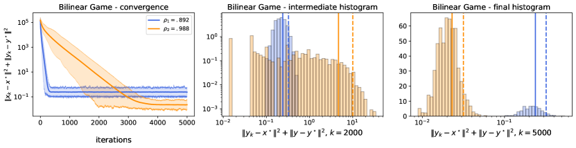
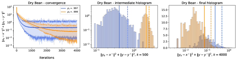
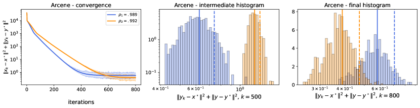
Figure 4: The figure shows the convergence behavior and distribution of performance scores for SAPD across three datasets. The left column displays the expected distance squared $E_{k}$ of SAPD iterates to the solution over iterations, while the middle and right columns show histograms of $E_{k}$ at fixed iterations. The continuous line in the convergence plots represents the average score $\mathcal{E}(E_{k})$, while the dashed line represents the $90^{th}$ percentile. The datasets include a synthetically generated bilinear game, and Dry Bean and Arcene from the UCI repository.

7 Conclusion

We consider a first-order primal-dual method that relies on stochastic estimates of the gradients for solving SCSC saddle point problems. We focused on the stochastic accelerated primal dual (SAPD) method Zhang et al. (2023).We obtained high-probability bounds for the iterates to lie in a given neighborhood of the saddle point that reflects accelerated behavior. For a class of quadratic SCSC problems subject to i.i.d. isotropic Gaussian noise and under a particular parameterization of the SAPD parameters, we were able to compute the distribution of the SAPD iterates exactly in closed form. We used this result to show that our high-probability bound is tight in terms of its dependency to target probability $p$, primal and dual stepsizes and the momentum parameter $\theta$. We also provide a risk-averse convergence analysis characterizing the “Conditional Value at Risk", $\chi^{2}$-divergences and the “Entropic Value at Risk" of the distance to the saddle point, highlighting the trade-offs between the bias and the risk associated with an approximate solution.

Acknowledgements

Yassine Laguel and Mert Gürbüzbalaban acknowledge support from the grants Office of Naval Research N00014-21-1-2244, National Science Foundation (NSF) CCF-1814888, NSF DMS1723085, NSF DMS-2053485. Necdet Serhat Aybat’s work was supported in part by the grant Office of Naval Research Award N00014-21-1-2271.

Appendix A Elementary proofs for subGaussians and convex risk measures

We provide in this section proofs of elementary properties of subGaussian vectors and convex risk measures.

A.1 Elementary Properties of Norm-subGaussian Vectors

In this section, we provide elementary proof of Lemma 2 and Lemma 3. The proofs follow from standard arguments that can be found in textbooks such as [8, 6].

A.1.1 Proof of Lemma 2

We follow standard arguments from [Vershynin, 2018]. First note that, for any $k>0$, we have

$$\begin{split}\operatorname{\mathbb{E}}[\|X\|^{k}]&=\int_{t=0}^{+\infty}\operatorname{\mathbb{P}}[\|X\|^{k}\geq t]\operatorname{\mathrm{d}}t=\int_{t=0}^{+\infty}\operatorname{\mathbb{P}}[\|X\|\geq t^{1/k}]\operatorname{\mathrm{d}}t\\ &\leq 2\int_{t=0}^{\infty}e^{-t^{\frac{2}{k}}/(2\sigma^{2})}\operatorname{\mathrm{d}}t=k(2\sigma^{2})^{\frac{k}{2}}\int_{u=0}^{\infty}e^{-u}u^{\frac{k}{2}-1}\operatorname{\mathrm{d}}u=k(2\sigma^{2})^{\frac{k}{2}}\Gamma\left(\frac{k}{2}\right),\end{split}$$

where $\Gamma$ denotes the gamma function. Hence, noting that $\Gamma(k)=(k-1)!$, by the monotone convergence theorem,

$$\begin{split}\operatorname{\mathbb{E}}[e^{\lambda\|X\|^{2}}]&=1+\sum_{k=1}^{\infty}\frac{\lambda^{k}}{k!}\operatorname{\mathbb{E}}[\|X\|^{2k}]\leq 1+\sum_{k=1}^{\infty}\frac{\lambda^{k}}{k!}(2k)(2\sigma^{2})^{k}\Gamma(k)\\ &\leq 1+2\sum_{k=1}^{\infty}\left(2\lambda\sigma^{2}\right)^{k}=\frac{2}{1-2\lambda\sigma^{2}}-1,\end{split}$$

the last equality being valid for any $\lambda\in[0,\frac{1}{2\sigma^{2}})$. Since for any $u\in[0,\frac{1}{2}]$, $\frac{1}{1-u}\leq e^{2u}$, we obtain $\mathbb{E}\left[e^{\lambda\|X\|^{2}}\right]\leq 2e^{4\lambda\sigma^{2}}-1$ for any $\lambda\in[0,\frac{1}{4\sigma^{2}}]$. Finally, last inequality follows from $2e^{2u}-1\leq e^{4u}$, where we chose $u=2\lambda\sigma^{2}$. $\square$

A.1.2 Proof of Lemma 3

For $u=0$, the inequality to prove is trivial. Assume $u\neq 0$. From Lemma 2 and Cauchy-Schwarz inequality, we have

$$\operatorname{\mathbb{E}}\left[e^{\lambda^{2}\langle u,X\rangle^{2}}\right]\leq\operatorname{\mathbb{E}}[e^{\lambda^{2}\|u\|^{2}\|X\|^{2}}]\leq e^{8\lambda^{2}\|u\|^{2}\sigma^{2}},$$ (A.1)

for all $\lambda\in[0,\frac{1}{2\sqrt{2}\sigma\|u\|}]$. Thus, for any such $\lambda$, noticing that $e^{t}\leq t+e^{t^{2}}$ for $t\in\operatorname{\mathbb{R}}$, we obtain $\operatorname{\mathbb{E}}\left[e^{\lambda\langle u,X\rangle}\right]\leq\operatorname{\mathbb{E}}\left[\lambda\langle u,X\rangle+e^{\lambda^{2}\langle u,X\rangle^{2}}\right]\leq e^{8\lambda^{2}\|u\|^{2}\sigma^{2}}$, where the second inequality follows from (A.1) and the assumption that $\operatorname{\mathbb{E}}[X]=0$. Moreover, for $\lambda\geq\frac{1}{2\sqrt{2}\|u\|\sigma}$, we have by Cauchy Schwarz’s inequality and Lemma 2 that $\operatorname{\mathbb{E}}[e^{\lambda\langle u,X\rangle}]\leq\operatorname{\mathbb{E}}\Big{[}e^{\frac{8\lambda^{2}\sigma^{2}\|u\|^{2}}{2}+\frac{\|X\|^{2}}{16\sigma^{2}}}\Big{]}\leq e^{\frac{1}{2}\left(1+8\lambda^{2}\sigma^{2}\|u\|^{2}\right)}\leq e^{8\lambda^{2}\|u\|^{2}\sigma^{2}}$, where the last inequality is due to $e^{\frac{1+t}{2}}\leq e^{t}$ for $t\geq 1$. $\square$

A.2 Elementary properties of Convex Risk Measures

The following lemma is used in the derivation of $\operatorname{CVaR}$ and $\operatorname{EVaR}$ bounds.

Lemma 21.

For any non-negative random variable $U\colon\Omega\to\operatorname{\mathbb{R}}_{+}$, we have for all $p\in[0,1)$:

$$\begin{split}{\color[rgb]{0,0,0}Q_{p}(U^{2})^{\frac{1}{2}}}{\color[rgb]{0,0,0}=Q_{p}(U)},\qquad\operatorname{CVaR}_{p}(U^{2})^{\frac{1}{2}}\geq\operatorname{CVaR}_{p}(U).\end{split}$$

Proof.

We first show that $Q_{p}(X^{2})=Q_{p}(X)^{2}$ for any $p\in(0,1)$. Indeed, for any $0\leq t<Q_{p}(U)^{2}$, we have $\operatorname{\mathbb{P}}[U^{2}\leq t]=\operatorname{\mathbb{P}}[U\leq\sqrt{t}]<p$ which follows from non-negativity of $U$ and definition of $Q_{p}(U)$. This implies $t<Q_{p}(U^{2})$; thus, $Q_{p}(U)^{2}\leq Q_{p}(U^{2})$. Conversely, we note that $p\leq\operatorname{\mathbb{P}}[U\leq Q_{p}(U)]=\operatorname{\mathbb{P}}[U^{2}\leq Q_{p}(U)^{2}]$, which implies $Q_{p}(U)^{2}\geq Q_{p}(U^{2})$; hence, $Q_{p}(X^{2})=Q_{p}(X)^{2}$. Using this result,

$$\begin{split}\operatorname{CVaR}_{p}(U^{2})=\left(\frac{1}{1-p}\int_{p^{\prime}=p}^{1}Q_{p^{\prime}}(U^{2})\mathrm{d}p^{\prime}\right)&=\operatorname{\mathbb{E}}_{p^{\prime}\sim\mathcal{U}[p,1]}[Q_{{\color[rgb]{0,0,0}p^{\prime}}}(U)^{2}]\\ &\geq\operatorname{\mathbb{E}}_{p^{\prime}\sim\mathcal{U}[p,1]}[Q_{p^{\prime}}(U)]^{2}=\operatorname{CVaR}_{p}(U)^{2},\end{split}$$

where $\mathcal{U}[p,1]$ denotes the uniform distribution on $[p,1]$, and the last inequality follows from the identity $\operatorname{\mathbb{E}}[X^{2}]=\operatorname{\mathbb{E}}[X]^{2}+\operatorname{\mathbb{E}}[(X-\operatorname{\mathbb{E}}[X])^{2}]$. ∎

Appendix B Intermediate results and proofs for the non-quadratic case

To start with, for the sake of completeness, we cite two results from [Zhang et al., 2023]. The first lemma is used to derive the almost sure bound result of Proposition 18, which is provided below in Appendix B.1, while the second lemma is used for deriving the convex inequalities provided in Appendix B.2.

Lemma 22 (See [Zhang et al., 2023, Lemma 1]).

The iterates $(x_{k},y_{k})$ of SAPD satisfy

$$\mathcal{L}\left(x_{k+1},\operatorname{y^{\star}}\right)-\mathcal{L}\left(\operatorname{x^{\star}},y_{k+1}\right)\leq -\left\langle q_{k+1},y_{k+1}-{\color[rgb]{0,0,0}\operatorname{y^{\star}}}\right\rangle+\theta\left\langle q_{k},y_{k}-{\color[rgb]{0,0,0}\operatorname{y^{\star}}}\right\rangle+\Lambda_{k}-\Sigma_{k+1}+\Gamma_{k+1}$$

$$+\langle\Delta_{k}^{x},{\color[rgb]{0,0,0}\operatorname{x^{\star}}-x_{k+1}}\rangle+\langle(1+\theta)\Delta_{k}^{y}-\theta\Delta_{{\color[rgb]{0,0,0}k-1}}^{y},y_{k+1}-\operatorname{y^{\star}}\rangle,$$

for all $k\geq 0$, where

$$q_{k}\operatorname{\triangleq} \operatorname{\nabla_{y}\operatorname{\Phi}}\left(x_{k},y_{k}\right)-\operatorname{\nabla_{y}\operatorname{\Phi}}\left(x_{k-1},y_{k-1}\right),\quad\Lambda_{k}\operatorname{\triangleq}\frac{1}{2\tau}\left\|\operatorname{x^{\star}}-x_{k}\right\|^{2}+\frac{1}{2\sigma}\left\|\operatorname{y^{\star}}-y_{k}\right\|^{2},$$

$$\Sigma_{k+1}\operatorname{\triangleq} \left(\frac{1}{2\tau}+\frac{\mu_{x}}{2}\right)\left\|\operatorname{x^{\star}}-x_{k+1}\right\|^{2}+\left(\frac{1}{2\sigma}+\frac{\mu_{y}}{2}\right)\left\|\operatorname{y^{\star}}-y_{k+1}\right\|^{2},$$

$$\Gamma_{k+1}\operatorname{\triangleq} \left(\frac{\operatorname{L_{xx}}}{2}-\frac{1}{2\tau}\right)\left\|x_{k+1}-x_{k}\right\|^{2}-\frac{1}{2\sigma}\left\|y_{k+1}-y_{k}\right\|^{2}+\theta\operatorname{L_{yx}}\left\|x_{k}-x_{k-1}\right\|\left\|y_{k+1}-y_{k}\right\|$$

$$+\theta\operatorname{L_{yy}}\left\|y_{k}-y_{k-1}\right\|\left\|y_{k+1}-y_{k}\right\|.$$

Lemma 23 (See [Zhang et al., 2023, Lemma 3]).

Let $(x_{n},y_{n})_{n\geq 0}$ denote the SAPD iterate sequence. Then, the following inequalities hold for all $n\in\operatorname{\mathbb{N}}$,

$$\|\operatorname{\hat{y}}_{n+1}-{\color[rgb]{0,0,0}y_{n+1}}\| \leq\frac{\sigma}{1+\sigma\mu_{y}}\left((1+\theta)\|\Delta_{n}^{y}\|+\theta\|\Delta_{n-1}^{y}\|\right),$$

$$\|\operatorname{\hat{\hat{x}}}_{n+1}-x_{n+1}\| \leq\frac{\tau}{1+\tau\mu_{x}}\left(\|\Delta_{n}^{x}\|+\operatorname{L_{xy}}\frac{\sigma}{1+\sigma\mu_{y}}\left((1+\theta)\|\Delta_{n}^{y}\|+\theta\|\Delta_{n-1}^{y}\|\right)\right),$$

$$\|\operatorname{\hat{\hat{y}}}_{n+1}-y_{n+1}\| \leq\frac{\sigma}{1+\sigma\mu_{y}}\begin{aligned} &\left(\frac{\tau(1+\theta)\operatorname{L_{yx}}}{1+\tau\mu_{x}}\|\Delta_{n-1}^{x}\|\right.+(1+\theta)\|\Delta_{n}^{y}\|\\ &\quad+\left(\theta+(1+\theta)\left(\frac{1+\sigma(1+\theta)\operatorname{L_{yy}}}{1+\sigma\mu_{y}}+\frac{\tau\sigma(1+\theta)\operatorname{L_{yx}}\operatorname{L_{xy}}}{(1+\tau\mu_{x})(1+\sigma\mu_{y})}\right)\right)\|\Delta_{n-1}^{y}\|\\ &\quad+\left.\theta\left(\frac{1+\sigma(1+\theta)\operatorname{L_{yy}}}{1+\sigma\mu_{y}}+\frac{\tau\sigma(1+\theta)\operatorname{L_{yx}}\operatorname{L_{xy}}}{(1+\tau\mu_{x})(1+\sigma\mu_{y})}\right)\|\Delta_{n-2}^{y}\|\right).\\ \end{aligned}$$

B.1 Proof of Proposition 18 (Almost sure domination of SAPD iterates)

Letting $\bar{x}_{n}\operatorname{\triangleq}K_{n}(\rho)^{-1}\sum_{k=0}^{n-1}\rho^{-k}x_{k+1}$, and $\bar{y}_{n}\operatorname{\triangleq}K_{n}(\rho)^{-1}\sum_{k=0}^{n-1}\rho^{-k}y_{k+1}$, with $K_{n}(\rho)\operatorname{\triangleq}{\color[rgb]{0,0,0}\sum_{k=0}^{n-1}}\rho^{-k}=\frac{1}{\rho^{n-1}}\times\frac{1-\rho^{n}}{1-\rho}$, by Jensen’s inequality , we have for all $\rho\in(0,1]$,

$$K_{n}(\rho)\left(\mathcal{L}\left(\bar{x}_{n},{\color[rgb]{0,0,0}\operatorname{y^{\star}}}\right)-\mathcal{L}\left({\color[rgb]{0,0,0}\operatorname{x^{\star}}},\bar{y}_{n}\right)\right)\leq\sum_{k=0}^{n-1}\rho^{-k}\left(\mathcal{L}\left(x_{k+1},{\color[rgb]{0,0,0}\operatorname{y^{\star}}}\right)-\mathcal{L}\left({\color[rgb]{0,0,0}\operatorname{x^{\star}}},y_{k+1}\right)\right).$$

Hence, in view of Lemma 22,

$$K_{n}(\rho)\left(\mathcal{L}\left(\bar{x}_{n},{\color[rgb]{0,0,0}\operatorname{y^{\star}}}\right)-\mathcal{L}\left({\color[rgb]{0,0,0}\operatorname{x^{\star}}},\bar{y}_{n}\right)\right)$$ (B.1)

$$\leq\sum_{k=0}^{n-1}\rho^{-k}{\color[rgb]{0,0,0}\Big{(}}-\left\langle q_{k+1},y_{k+1}-{\color[rgb]{0,0,0}\operatorname{y^{\star}}}\right\rangle+\theta\left\langle q_{k},y_{k}-{\color[rgb]{0,0,0}\operatorname{y^{\star}}}\right\rangle+\Lambda_{k}-\Sigma_{k+1}+\Gamma_{k+1}$$

$$\quad+\langle\Delta_{k}^{x},\operatorname{x^{\star}}-x_{k+1}\rangle+\langle(1+\theta)\Delta_{k}^{y}-\theta\Delta_{k-1}^{y},y_{k+1}-\operatorname{y^{\star}}\rangle{\color[rgb]{0,0,0}\Big{)}},$$

where $q_{k}\operatorname{\triangleq}\operatorname{\nabla_{y}\operatorname{\Phi}}(x_{k},y_{k})-\operatorname{\nabla_{y}\operatorname{\Phi}}(x_{k-1},y_{k-1})$. By Cauchy-Schwarz inequality, observe that

$$\left|\left\langle q_{k+1},y_{k+1}-{\color[rgb]{0,0,0}\operatorname{y^{\star}}}\right\rangle\right|\leq S_{k+1}\operatorname{\triangleq}\operatorname{L_{yx}}\left\|x_{k+1}-x_{k}\right\|\left\|y_{k+1}-y\right\|+\operatorname{L_{yy}}\left\|y_{k+1}-y_{k}\right\|\left\|y_{k+1}-{\color[rgb]{0,0,0}\operatorname{y^{\star}}}\right\|,\quad\forall k\geq 0.$$

Hence, using $q_{0}=\mathbf{0}$ due to our initialization of $(x_{-1},y_{-1})=(x_{0},y_{0})$, we have

$$\sum_{k=0}^{n-1}\rho^{-k}\left(-\left\langle q_{k+1},y_{k+1}-{\color[rgb]{0,0,0}\operatorname{y^{\star}}}\right\rangle+\theta\left\langle q_{k},y_{k}-{\color[rgb]{0,0,0}\operatorname{y^{\star}}}\right\rangle\right)=\sum_{k=0}^{n-2}\rho^{-k}\left(\frac{\theta}{\rho}-1\right)\left\langle q_{k+1},y_{k+1}-{\color[rgb]{0,0,0}\operatorname{y^{\star}}}\right\rangle-\rho^{-n+1}\left\langle q_{n},y_{n}-{\color[rgb]{0,0,0}\operatorname{y^{\star}}}\right\rangle$$

$$\leq\sum_{k=0}^{n-2}\rho^{-k}\left|1-\frac{\theta}{\rho}\right|S_{k+1}+\rho^{-n+1}S_{n}{\color[rgb]{0,0,0}\leq}\sum_{k=0}^{n-1}\rho^{-k}\left|1-\frac{\theta}{\rho}\right|S_{k+1}+\rho^{-n+1}\frac{\theta}{\rho}S_{n}.$$

From (B.1), it follows that

$$K_{n}(\rho)\left(\mathcal{L}\left(\bar{x}_{n},{\color[rgb]{0,0,0}\operatorname{y^{\star}}}\right)-\mathcal{L}\left({\color[rgb]{0,0,0}\operatorname{x^{\star}}},\bar{y}_{n}\right)\right)+\rho^{-n+1}\mathcal{E}_{n}$$

$$\leq U_{n}+\sum_{k=0}^{n-1}\rho^{-k}{\color[rgb]{0,0,0}\Big{(}}\langle\Delta_{k}^{x},\operatorname{x^{\star}}-x_{k+1}\rangle+\langle(1+\theta)\Delta_{k}^{y}-\theta\Delta_{k-1}^{y},y_{k+1}-\operatorname{y^{\star}}\rangle{\color[rgb]{0,0,0}\Big{)}},$$

where $U_{n}\triangleq\sum_{k=0}^{n-1}\rho^{-k}\left(\Gamma_{k+1}+\Lambda_{k}-\Sigma_{k+1}+\left|1-\frac{\theta}{\rho}\right|S_{k+1}\right)-\rho^{-n+1}\left(-\mathcal{E}_{n}-\frac{\theta}{\rho}S_{n}\right)$. Now, observe that for all $n\geq 1$,

$$U_{n} =\frac{1}{2}\sum_{k=0}^{n-1}\rho^{-k}\left(\xi_{k}^{\top}A\xi_{k}-\xi_{k+1}^{\top}B\xi_{k+1}\right)-\rho^{-n+1}\left(-\mathcal{E}_{n}-\frac{\theta}{\rho}S_{n}\right)$$

$$=\frac{1}{2}\xi_{0}^{\top}A\xi_{0}-\frac{1}{2}\sum_{k=1}^{n-1}\rho^{-k+1}\left[\xi_{k}^{\top}\left(B-\frac{1}{\rho}A\right)\xi_{k}\right]-\rho^{-n+1}\left(\frac{1}{2}\xi_{n}^{\top}B\xi_{n}-\mathcal{E}_{n}-\frac{\theta}{\rho}S_{n}\right),$$

where $A,B\in\mathbb{R}^{5\times 5}$ and $\xi_{k}\in\mathbb{R}^{5}$ are defined for $k\geq 0$ as

$$A\triangleq\left(\begin{array}[]{ccccc}\frac{1}{\tau}&0&0&0&0\\ 0&\frac{1}{\sigma}&0&0&0\\ 0&0&0&0&\theta\operatorname{L_{yx}}\\ 0&0&0&0&\theta\operatorname{L_{yy}}\\ 0&0&\theta\operatorname{L_{yx}}&\theta\operatorname{L_{yy}}&-\alpha\end{array}\right),\leavevmode\nobreak\ B\triangleq\left(\begin{array}[]{ccccc}\frac{1}{\tau}+\mu_{x}&0&0&0&0\\ 0&\frac{1}{\sigma}+\mu_{y}&-\left|1-\frac{\theta}{\rho}\right|\operatorname{L_{yx}}&-\left|1-\frac{\theta}{\rho}\right|\operatorname{L_{yy}}&0\\ 0&-\left|1-\frac{\theta}{\rho}\right|\operatorname{L_{yx}}&\frac{1}{\tau}-\operatorname{L_{xx}}&0&0\\ 0&-\left|1-\frac{\theta}{\rho}\right|\operatorname{L_{yy}}&0&\frac{1}{\sigma}-\alpha&0\\ 0&0&0&0&0\end{array}\right),$$

and $\xi_{k}\triangleq\left(\begin{array}[]{ccccc}\left\|x_{k}-{\color[rgb]{0,0,0}\operatorname{x^{\star}}}\right\|,&\left\|y_{k}-{\color[rgb]{0,0,0}\operatorname{y^{\star}}}\right\|.&\left\|x_{k}-x_{k-1}\right\|,&\left\|y_{k}-y_{k-1}\right\|,&\left\|y_{k+1}-y_{k}\right\|\end{array}\right)^{\top}\in\mathbb{R}^{5}$. By [Zhang et al., 2023, Lemma 5], the matrix inequality condition (2.2) is equivalent to having $B-\rho^{-1}A\succeq 0$. In this case, we almost surely have

$$U_{n}\leq\frac{1}{2}\xi_{0}^{\top}A\xi_{0}-\rho^{-n+1}\left(\frac{1}{2}\xi_{n}^{\top}B\xi_{n}-\mathcal{E}_{n}-\frac{\theta}{\rho}S_{n}\right).$$ (B.2)

Finally, denoting

$$G^{\prime\prime}\operatorname{\triangleq}\left(\begin{array}[]{ccc}\frac{1}{\sigma}\left(1-\frac{1}{\rho}\right)+\mu_{y}+\frac{\alpha}{\rho}&\left(-\left|1-\frac{\theta}{\rho}\right|-\frac{\theta}{\rho}\right)\operatorname{L_{yx}}&\left(-\left|1-\frac{\theta}{\rho}\right|-\frac{\theta}{\rho}\right)\operatorname{L_{yy}}\\ \left(-\left|1-\frac{\theta}{\rho}\right|-\frac{\theta}{\rho}\right)\operatorname{L_{yx}}&\frac{1}{\tau}-\operatorname{L_{xx}}&0\\ \left(-\left|1-\frac{\theta}{\rho}\right|-\frac{\theta}{\rho}\right)\operatorname{L_{yy}}&0&\frac{1}{\sigma}-\alpha\end{array}\right),$$

we have $G^{\prime\prime}\succeq 0$ in view of [Zhang et al., 2023, Lemma 6]; thus,

$$\frac{1}{2}\xi_{n}^{\top}B\xi_{n}-\frac{\theta}{\rho}S_{n} = \frac{1}{2\rho\tau}\left\|x_{n}-x\right\|^{2}+\frac{1}{2}\left(\frac{1}{\rho\sigma}-\frac{\alpha}{\rho}\right)\left\|y_{n}-y\right\|^{2}+\frac{1}{2}\xi_{n}^{\top}\left(\begin{array}[]{ccc}\frac{1}{\tau}\left(1-\frac{1}{\rho}\right)+\mu_{x}&\mathbf{0}_{1\times 3}&0\\ \mathbf{0}_{3\times 1}&G^{\prime\prime}&\mathbf{0}_{3\times 1}\\ 0&\mathbf{0}_{1\times 3}&0\end{array}\right)\xi_{n}$$

$$\geq \frac{1}{2\rho\tau}\left\|x_{n}-x\right\|^{2}+\frac{1}{2\rho\sigma}(1-\alpha\sigma)\left\|y_{n}-y\right\|^{2}=\mathcal{E}_{n}.$$

Therefore, using (B.2), we can conclude that $U_{n}\leq\frac{1}{2}\xi_{0}^{\top}A\xi_{0}{\color[rgb]{0,0,0}\leq}\frac{1}{2\tau}\|{\color[rgb]{0,0,0}x_{0}}-\operatorname{x^{\star}}\|^{2}+\frac{1}{2\sigma}\|{\color[rgb]{0,0,0}y_{0}}-\operatorname{y^{\star}}\|^{2}=\mathcal{D}_{\tau,\sigma}$. Finally, by non-negativity of $\mathcal{L}\left(\bar{x}_{n},{\color[rgb]{0,0,0}\operatorname{y^{\star}}}\right)-\mathcal{L}\left({\color[rgb]{0,0,0}\operatorname{x^{\star}}},\bar{y}_{n}\right)$, we obtain (5.15). $\square$

B.2 Convex inequalities

B.2.1 Proof of Lemma 19

We first start with a technical result we will use in the proof of Lemma 19.

Lemma 24.

For any $n\geq 1$,

$$\|\operatorname{\hat{\hat{y}}}_{n+1}-\operatorname{y^{\star}}\|\leq{\|A_{0}\|(\mathcal{E}_{n}+\mathcal{E}_{n-1})^{1/2}}+\frac{1}{1+\sigma\mu_{y}}\left(\left(1+\sigma(1+\theta)\operatorname{L_{yy}}\right)\|y_{n}-\operatorname{\hat{y}}_{n}\|+\sigma(1+\theta)\operatorname{L_{yx}}\|x_{n}-\operatorname{\hat{\hat{x}}}_{n}\|\right),$$

where $\operatorname{\hat{\hat{y}}}_{n+1},\operatorname{\hat{y}}_{n},\operatorname{\hat{\hat{x}}}_{n}$ are defined in (5.12), and $A_{0}\in\mathbb{R}^{4}$ is defined as

$$A_{0}\operatorname{\triangleq}{\color[rgb]{0,0,0}\tfrac{1}{1+\sigma\mu_{y}}}\begin{bmatrix}\sqrt{2\rho\tau}\sigma(1+\theta)\operatorname{L_{yx}}\\ \frac{\sqrt{2\rho\sigma}}{\sqrt{1-\alpha\sigma}}(1+\sigma(1+\theta)\operatorname{L_{yy}})\\ {\sqrt{2\rho\tau}\cdot\sigma\theta\operatorname{L_{yx}}}\\ {\frac{\sqrt{2\rho\sigma}}{\sqrt{(1-\alpha\sigma)}}\cdot\sigma\theta\operatorname{L_{yy}}}\end{bmatrix}\in\operatorname{\mathbb{R}}^{4}.$$

Proof.

Since $(\operatorname{x^{\star}},\operatorname{y^{\star}})$ is a solution of (1.1), $\operatorname{x^{\star}}$ and $\operatorname{y^{\star}}$ are fixed points of two deterministic proximal gradient maps, i.e.,

$$\operatorname{x^{\star}}=\text{prox}_{\tau f}\left(\operatorname{x^{\star}}-\tau\operatorname{\nabla_{x}\operatorname{\Phi}}(\operatorname{x^{\star}},\operatorname{y^{\star}})\right),\quad\operatorname{y^{\star}}=\text{prox}_{\sigma g}\left(\operatorname{y^{\star}}+\sigma\operatorname{\nabla_{y}\operatorname{\Phi}}(\operatorname{x^{\star}},\operatorname{y^{\star}})\right).$$ (B.4)

Thus, by the contraction properties of the prox for strongly convex functions, and convexity of the squared norm, we have

$$\begin{split}\|\operatorname{\hat{\hat{y}}}_{n+1}-\operatorname{y^{\star}}\|\leq\frac{1}{1+\sigma\mu_{y}}\left\|\operatorname{\hat{y}}_{n}+\sigma(1+\theta)\operatorname{\nabla_{y}\operatorname{\Phi}}(\operatorname{\hat{\hat{x}}}_{n},\operatorname{\hat{y}}_{n})-\sigma\theta\operatorname{\nabla_{y}\operatorname{\Phi}}(x_{n-1},{\color[rgb]{0,0,0}y_{n-1}})-\operatorname{y^{\star}}-\sigma\operatorname{\nabla_{y}\operatorname{\Phi}}(\operatorname{x^{\star}},\operatorname{y^{\star}})\right\|.\end{split}$$

By the triangular inequality and smoothness assumptions on $\operatorname{\nabla_{y}\operatorname{\Phi}}$, we deduce

The statement finally follows from Cauchy-Schwarz inequality. ∎

Now we are ready to prove Lemma 19. By Young’s inequality, for any $\gamma_{x},\gamma_{y}>0$,

$$\begin{split}{\frac{-1}{1+\rho}}&{\left({P}_{n}^{(1)}+\langle\Delta_{n}^{x},\operatorname{\hat{\hat{x}}}_{n+1}-x_{n+1}\rangle+(1+\theta)\;\langle\Delta_{n}^{y},y_{n+1}-\operatorname{\hat{y}}_{n+1}\rangle\right)}\\ &=\frac{1}{1+\rho}\begin{aligned} &\left(\langle\Delta_{n}^{x},\operatorname{\hat{\hat{x}}}_{n+1}-\operatorname{x^{\star}}\rangle+(1+\theta)\;\langle\Delta_{n}^{y},\operatorname{y^{\star}}-\operatorname{\hat{y}}_{n+1}\rangle\right.\\ &\left.-\langle\Delta_{n}^{x},\operatorname{\hat{\hat{x}}}_{n+1}-x_{n+1}\rangle-(1+\theta)\;\langle\Delta_{n}^{y},y_{n+1}-\operatorname{\hat{y}}_{n+1}\rangle\right)\\ \end{aligned}\\ &=\frac{1}{1+\rho}\left(\langle\Delta_{n}^{x},x_{n+1}-\operatorname{x^{\star}}\rangle+(1+\theta)\langle\Delta_{n}^{y},\operatorname{y^{\star}}-y_{n+1}\rangle\right)\\ &\leq\frac{\gamma_{x}}{2(1+\rho)}\|\Delta_{n}^{x}\|^{2}+\frac{1}{2\gamma_{x}(1+\rho)}\|\operatorname{x^{\star}}-x_{n+1}\|^{2}+\frac{(1+\theta)\gamma_{y}}{2(1+\rho)}\|\Delta_{n}^{y}\|^{2}+\frac{(1+\theta)}{2\gamma_{y}(1+\rho)}\|y_{n+1}-\operatorname{y^{\star}}\|^{2}.\end{split}$$

Setting $\gamma_{x}\operatorname{\triangleq}8\tau$ and $\gamma_{y}\operatorname{\triangleq}\frac{8\sigma(1+\theta)}{1-\alpha\sigma}$, we ensure that

$$\begin{split}\frac{-1}{1+\rho}\left({P}_{n}^{(1)}+\langle\Delta_{n}^{x},\operatorname{\hat{\hat{x}}}_{n+1}-x_{n+1}\rangle\right.&+\left.(1+\theta)\;\langle\Delta_{n}^{y},y_{n+1}-\operatorname{\hat{y}}_{n+1}\rangle\right)\\ &\leq\frac{\rho}{8(1+\rho)}\mathcal{E}_{n+1}+\frac{4\tau}{1+\rho}\|\Delta_{n}^{x}\|^{2}+\frac{4\sigma(1+\theta)^{2}}{(1+\rho)(1-\alpha\sigma)}\|\Delta_{n}^{y}\|^{2},\\ \end{split}$$ (B.5)

where $\mathcal{E}_{n}=\mathcal{D}_{n}/\rho$ and $\mathcal{D}_{n}$ is defined in (2.4). Moreover, we also have $\frac{-\rho}{1+\rho}{P}_{n-1}^{(2)}+\frac{\theta}{1+\rho}\langle\Delta_{n-1}^{y},y_{n+1}-\operatorname{\hat{\hat{y}}}_{n+1}\rangle=\frac{\theta}{1+\rho}\langle\Delta_{n-1}^{y},y_{n+1}-\operatorname{y^{\star}}\rangle\leq\frac{\theta}{1+\rho}\left(\frac{\gamma^{\prime}_{y}}{2}\|\Delta_{n-1}^{y}\|^{2}+\frac{1}{2\gamma^{\prime}_{y}}\|\operatorname{y^{\star}}-y_{n+1}\|^{2}\right)$ for any $\gamma^{\prime}_{y}>0$. Hence, setting $\gamma^{\prime}_{y}=\frac{8\theta\sigma}{1-\alpha\sigma}$ leads to

$$\begin{split}{\frac{-\rho}{1+\rho}}{P}_{n-1}^{(2)}+\frac{\theta}{1+\rho}\langle\Delta_{n-1}^{y},y_{n+1}-\operatorname{\hat{\hat{y}}}_{n+1}\rangle\leq\frac{\rho}{8(1+\rho)}\mathcal{E}_{n+1}+\frac{4\sigma\theta^{2}}{(1+\rho)(1-\alpha\sigma)}\|\Delta_{n-1}^{y}\|^{2}.\end{split}$$ (B.6)

Finally, observe that for any $\gamma>0$,

$$\begin{split}-{P}_{n}^{(2)}&\leq\frac{\theta\gamma}{2\rho}{\|\Delta_{n}^{y}\|^{2}}+\frac{\theta}{2\gamma\rho}\|\operatorname{\hat{\hat{y}}}_{n+2}-\operatorname{y^{\star}}\|^{2}\\ &\leq\frac{\theta\gamma}{2\rho}{\|\Delta_{n}^{y}\|^{2}}+\frac{\theta}{2\gamma\rho}\bigg{(}3\|A_{0}\|^{2}(\mathcal{E}_{n+1}+\mathcal{E}_{n})\begin{aligned} &+3\Big{(}\frac{1+\sigma(1+\theta)\operatorname{L_{yy}}}{1+\sigma\mu_{y}}\Big{)}^{2}\|\operatorname{\hat{y}}_{n+1}-y_{n+1}\|^{2}\\ &+3\Big{(}\frac{\sigma(1+\theta)\operatorname{L_{yx}}}{1+\sigma\mu_{y}}\Big{)}^{2}\|\operatorname{\hat{\hat{x}}}_{n+1}-x_{n+1}\|^{2}\bigg{)},\end{aligned}\\ \end{split}$$

where the last inequality follows from Lemma 24 and the simple inequality $(a+b+c)^{2}\leq 3a^{2}+3b^{2}+3c^{2}$ for any $a,b,c\in\mathbb{R}$. Setting $\gamma\operatorname{\triangleq}\frac{6\theta\|A_{0}\|^{2}(1+\rho)}{{\color[rgb]{0,0,0}\rho^{2}}}$ ensures that

$$-{P}_{n}^{(2)}\leq\frac{\rho}{4(1+\rho)}(\mathcal{E}_{n+1}+\mathcal{E}_{n})\begin{aligned} &+\frac{3{\color[rgb]{0,0,0}\theta^{2}}\|A_{0}\|^{2}(1+\rho)}{{\color[rgb]{0,0,0}\rho^{3}}}\|\Delta_{n}^{y}\|^{2}\\ &+\frac{\rho}{4\|A_{0}\|^{2}(1+\rho)}\left(\frac{1+\sigma(1+\theta)\operatorname{L_{yy}}}{1+\sigma\mu_{y}}\right)^{2}\|\operatorname{\hat{y}}_{n+1}-y_{n+1}\|^{2}\\ &+\frac{\rho}{4\|A_{0}\|^{2}(1+\rho)}\left(\frac{\sigma(1+\theta)\operatorname{L_{yx}}}{1+\sigma\mu_{y}}\right)^{2}\|\operatorname{\hat{\hat{x}}}_{n+1}-x_{n+1}\|^{2}.\end{aligned}$$ (B.7)

Hence, using the trivial upper bound $\mathcal{E}_{n+1}\leq(\mathcal{E}_{n+1}+\mathcal{E}_{n})$ and combining the bounds eqs. B.5, B.6 and B.7 we obtained above, we get

$$\begin{split}\frac{-1}{1+\rho}&{P}_{n}^{(1)}-{P}_{n}^{(2)}-\frac{\rho}{1+\rho}{P}_{n-1}^{(2)}-\frac{1}{1+\rho}Q_{n}\\ &\leq\begin{aligned} &\frac{\rho}{2(1+\rho)}(\mathcal{E}_{n+1}+\mathcal{E}_{n})\\ &+\frac{4\tau}{1+\rho}\|\Delta_{n}^{x}\|^{2}+\frac{4\sigma(1+\theta)^{2}}{(1+\rho)(1-\alpha\sigma)}\|\Delta_{n}^{y}\|^{2}+\frac{4\sigma\theta^{2}}{(1+\rho)(1-\alpha\sigma)}\|\Delta_{n-1}^{y}\|^{2}+\frac{3\theta^{2}(1+\rho)\|A_{0}\|^{2}}{\rho^{3}}{\|\Delta_{n}^{y}\|^{2}}\\ &+\frac{\rho}{4\|A_{0}\|^{2}(1+\rho)}\left(\frac{1+\sigma(1+\theta)\operatorname{L_{yy}}}{1+\sigma\mu_{y}}\right)^{2}\|\operatorname{\hat{y}}_{n+1}-y_{n+1}\|^{2}\\ &+\frac{\rho}{4\|A_{0}\|^{2}(1+\rho)}\left(\frac{\sigma(1+\theta)\operatorname{L_{yx}}}{1+\sigma\mu_{y}}\right)^{2}\|\operatorname{\hat{\hat{x}}}_{n+1}-x_{n+1}\|^{2}.\end{aligned}\end{split}$$

Let us now introduce $\zeta_{k}\operatorname{\triangleq}\Big{[}\|\Delta_{k}^{x}\|,\;\|\Delta_{k}^{y}\|,\;\rho^{1/2}\|\Delta_{k-1}^{y}\|\Big{]}^{\top}{\color[rgb]{0,0,0}\in\mathbb{R}^{3}}$ for $k\geq 0$; then, by similar computations the following bounds follow from Lemma 23:

$$\begin{split}\|\operatorname{\hat{y}}_{n+1}-y_{n+1}\|^{2}&\leq\zeta_{n}^{\top}\operatorname{\text{Diag}}\left[0,\frac{2\sigma^{2}(1+\theta)^{2}}{(1+\sigma\mu_{y})^{2}},\frac{2\sigma^{2}{\theta^{2}\rho^{-1}}}{(1+\sigma\mu_{y})^{2}}\right]\zeta_{n}\\ \|\operatorname{\hat{\hat{x}}}_{n+1}-x_{n+1}\|^{2}&\leq\zeta_{n}^{\top}\operatorname{\text{Diag}}\left[\frac{3\tau^{2}}{(1+\tau\mu_{x})^{2}},\frac{3\tau^{2}\sigma^{2}(1+\theta)^{2}\operatorname{L_{xy}}^{2}}{(1+\tau\mu_{x})^{2}(1+\sigma\mu_{y})^{2}},\frac{3\tau^{2}\sigma^{2}\theta^{2}\rho^{-1}\operatorname{L_{xy}}^{2}}{(1+\tau\mu_{x})^{2}(1+\sigma\mu_{y})^{2}}\right]\zeta_{n},\end{split}$$

and we deduce that

$$\frac{-1}{1+\rho}{P}_{n}^{(1)}-{P}_{n}^{(2)}-\frac{\rho}{1+\rho}{P}_{n-1}^{(2)}-\frac{1}{1+\rho}Q_{n}\leq\frac{\rho}{2(1+\rho)}(\mathcal{E}_{n+1}+\mathcal{E}_{n})+\zeta_{n}^{\top}\operatorname{\text{Diag}}\left[B^{x},B^{y},B_{-1}^{y}\right]\zeta_{n}$$

where $B^{x},B^{y},B_{-1}^{y}$ are constants specified in Table 2 of Appendix D.

We now treat the sum $\sum_{k=0}^{n}\rho^{n-k}{\color[rgb]{0,0,0}Q_{k}}$. Observe first that for all $n\in\operatorname{\mathbb{N}}$, Lemma 23,

$$\begin{split}Q_{n}&\leq\|\Delta_{n}^{x}\|\;\|\operatorname{\hat{\hat{x}}}_{n+1}-x_{n+1}\|+(1+\theta)\|\Delta_{n}^{y}\|\;\|y_{n+1}-\operatorname{\hat{y}}_{n+1}\|+\theta\;\|\Delta_{n-1}^{y}\|\;\|y_{n+1}{\color[rgb]{0,0,0}-}\operatorname{\hat{\hat{y}}}_{n+1}\|\\ &\leq\begin{aligned} &\|\Delta_{n}^{x}\|\;\left[\frac{\tau}{1+\tau\mu_{x}}\left(\left\|\Delta_{n}^{x}\right\|+\operatorname{L_{xy}}\frac{\sigma}{1+\sigma\mu_{y}}\left((1+\theta)\left\|\Delta_{n}^{y}\right\|+\theta\left\|\Delta_{n-1}^{y}\right\|\right)\right)\right]\\ &+(1+\theta)\|\Delta_{n}^{y}\|\;{\left(\frac{\sigma}{1+\sigma\mu_{y}}\left((1+\theta)\|\Delta_{n}^{y}\|+\theta\|\Delta_{n-1}^{y}\|\right)\right)}\\ &+\theta\|\Delta_{n-1}^{y}\|\frac{\sigma}{1+\sigma\mu_{y}}\begin{aligned} &\left(\frac{\tau(1+\theta)\operatorname{L_{yx}}}{1+\tau\mu_{x}}\|\Delta_{n-1}^{x}\|\right.\\ &+(1+\theta)\|\Delta_{n}^{y}\|\\ &+\left(\theta+(1+\theta)\left(\frac{1+\sigma(1+\theta)\operatorname{L_{yy}}}{1+\sigma\mu_{y}}+\frac{\tau\sigma(1+\theta)\operatorname{L_{yx}}\operatorname{L_{xy}}}{(1+\tau\mu_{x})(1+\sigma\mu_{y})}\right)\right)\|\Delta_{n-1}^{y}\|\\ &+\left.\theta\left(\frac{1+\sigma(1+\theta)\operatorname{L_{yy}}}{1+\sigma\mu_{y}}+\frac{\tau\sigma(1+\theta)\operatorname{L_{yx}}\operatorname{L_{xy}}}{(1+\tau\mu_{x})(1+\sigma\mu_{y})}\right)\|\Delta_{n-2}^{y}\|\right),\\ \end{aligned}\end{aligned}\\ \end{split}$$

which, after organizing the terms and using $ab\leq a^{2}/2+b^{2}/2$ for any scalars $a,b$, becomes

$$\begin{split}Q_{n}&\leq\begin{aligned} &\frac{\tau}{1+\tau\mu_{x}}\|\Delta_{n}^{x}\|^{2}+\frac{\sigma(1+\theta)^{2}}{1+\sigma\mu_{y}}\|\Delta_{n}^{y}\|^{2}\\ &+\frac{\sigma\theta}{1+\sigma\mu_{\mathbf{y}}}\left(\theta+(1+\theta)\left(\frac{1+\sigma(1+\theta)\mathrm{L}_{\mathrm{yy}}}{1+\sigma\mu_{y}}+\frac{\tau\sigma(1+\theta)\mathrm{L}_{\mathrm{yx}}\mathrm{L}_{\mathrm{xy}}}{\left(1+\tau\mu_{x}\right)\left(1+\sigma\mu_{y}\right)}\right)\right)\|\Delta_{n-1}^{y}\|^{2}\\ &+\frac{\sigma\theta}{{\color[rgb]{0,0,0}2}(1+\sigma\mu_{y})}\quad\frac{\tau(1+\theta)\operatorname{L_{yx}}}{1+\tau\mu x}\|\Delta_{n-1}^{y}\|^{2}+\frac{\sigma\theta}{{\color[rgb]{0,0,0}2}(1+\sigma\mu_{y})}\frac{\tau(1+\theta)\operatorname{L_{yx}}}{1+\tau\mu_{x}}\|\Delta_{n-1}^{x}\|^{2}\\ &+\frac{\sigma\theta}{1+\sigma\mu y}(1+\theta)\|\Delta_{n}^{y}\|^{2}+\frac{\sigma\theta}{1+\sigma\mu_{y}}(1+\theta)\|\Delta_{n-1}^{y}\|^{2}\\ &+\frac{\sigma\theta}{1+\sigma\mu_{y}}{\color[rgb]{0,0,0}\frac{\theta}{2}}\left(\frac{1+\sigma(1+\theta)\mathrm{L}_{\mathrm{yy}}}{1+\sigma\mu_{y}}+\frac{\tau\sigma(1+\theta)\mathrm{L}_{\mathrm{yx}}\mathrm{L}_{\mathrm{xy}}}{\left(1+\tau\mu_{x}\right)\left(1+\sigma\mu_{y}\right)}\right)\|\Delta_{n-1}^{y}\|^{2}\\ &\quad+\frac{\sigma\theta}{1+\sigma\mu_{y}}{\color[rgb]{0,0,0}\frac{\theta}{2}}\left(\frac{1+\sigma(1+\theta)\mathrm{L}_{\mathrm{yy}}}{1+\sigma\mu_{y}}+\frac{\tau\sigma(1+\theta)\mathrm{L}_{\mathrm{yx}}\mathrm{L}_{\mathrm{xy}}}{\left(1+\tau\mu_{x}\right)\left(1+\sigma\mu_{y}\right)}\right)\|\Delta_{n-2}^{y}\|^{2}\\ &+\frac{\tau\sigma(1+\theta)\operatorname{L_{xy}}}{{\color[rgb]{0,0,0}2}\left(1+\tau\mu_{x}\right)\left(1+\tau\mu_{y}\right)}\|\Delta_{n}^{x}\|^{2}+\frac{\tau\sigma(1+\theta)\operatorname{L_{xy}}}{{\color[rgb]{0,0,0}2}\left(1+\tau\mu_{x}\right)\left(1+\tau\mu_{y}\right)}\|\Delta_{n}^{y}\|^{2}\\ &+\frac{\tau\sigma\theta\operatorname{L_{xy}}}{{\color[rgb]{0,0,0}2}\left(1+\tau\mu_{x}\right)\left(1+\tau\mu_{y}\right)}\|\Delta_{n}^{x}\|^{2}+\frac{\tau\sigma\theta\operatorname{L_{xy}}}{{\color[rgb]{0,0,0}2}\left(1+\tau\mu_{x}\right)\left(1+\tau\mu_{y}\right)}\|\Delta_{n-1}^{y}\|^{2}\\ \end{aligned}\\ \end{split}$$

Thus, we obtain $Q_{n}\leq C^{x}\;\|\Delta_{n}^{x}\|^{2}\;+\;C_{-1}^{x}\;\rho\|\Delta_{n-1}^{x}\|^{2}\;+\;C^{y}\;\|\Delta_{n}^{y}\|^{2}\;+\;C_{-1}^{y}\;\rho\|\Delta_{n-1}^{y}\|^{2}\;+\;C_{-2}^{y}\;\rho^{2}\|\Delta_{n-2}^{y}\|^{2}$ for some constants $C^{x},C_{-1}^{x},C^{y},C_{-1}^{y},C_{-2}^{y}$ (that are explicitly given in Table 2 of Appendix D). Hence, setting $\Delta_{-1}^{x}=\Delta_{-1}^{y}=\Delta_{-2}^{x}=0$, we obtain,

$$\begin{split}\sum_{k=0}^{n}\rho^{n-k}Q_{k}&-\frac{1}{1+\rho}{P}_{n}^{(1)}-{P}_{n}^{(2)}-\frac{\rho}{1+\rho}{P}_{n-1}^{(2)}-\frac{1}{1+\rho}Q_{n}\\ &\leq\begin{aligned} \frac{\rho}{2({\color[rgb]{0,0,0}1}+\rho)}(\mathcal{E}_{n+1}+\mathcal{E}_{n})&+\sum_{k=0}^{n}\rho^{n-k}\begin{aligned} (&C^{x}\|\Delta_{k}^{x}\|^{2}+C_{-1}^{x}\rho\|\Delta_{k-1}^{x}\|^{2}\\ &+C^{y}\|\Delta_{k}^{y}\|^{2}+C_{-1}^{y}\rho\|\Delta_{k-1}^{y}\|^{2}+C_{-2}^{y}\rho^{2}\|\Delta_{k-2}^{y}\|^{2})\\ \end{aligned}\\ &+B^{x}\|\Delta_{n}^{x}\|^{2}+B^{y}\|\Delta_{n}^{y}\|^{2}+B_{-1}^{y}\rho\|\Delta_{n-1}^{y}\|^{2};\end{aligned}\\ \end{split}$$

therefore, rearranging the terms together we get

$$\begin{split}\sum_{k=0}^{n}\rho^{n-k}Q_{k}&-\frac{1}{1+\rho}{P}_{n}^{(1)}-{P}_{n}^{(2)}-\frac{\rho}{1+\rho}{P}_{n-1}^{(2)}-\frac{1}{1+\rho}Q_{n}\\ &\leq\begin{aligned} &\frac{\rho}{2({\color[rgb]{0,0,0}1}+\rho)}(\mathcal{E}_{n+1}+\mathcal{E}_{n})\\ &+C^{x}\sum_{k=0}^{n}\rho^{n-k}\|\Delta_{k}^{x}\|^{2}+C_{-1}^{x}\sum_{k=0}^{n-1}\rho^{n-k}\|\Delta_{k}^{x}\|^{2}+C^{y}\sum_{k=0}^{n}\rho^{n-k}\|\Delta_{k}^{y}\|^{2}\\ &+C_{-1}^{y}\sum_{k=0}^{n-1}\rho^{n-k}\|\Delta_{k}^{y}\|^{2}+C_{-2}^{y}\sum_{k=0}^{n-2}\rho^{n-k}\|\Delta_{k}^{y}\|^{2}+B^{x}\|\Delta_{n}^{x}\|^{2}+B^{y}\|\Delta_{n}^{y}\|^{2}+B_{-1}^{y}\rho\|\Delta_{n-1}^{y}\|^{2}\end{aligned}\\ &\leq\frac{\rho}{2({\color[rgb]{0,0,0}1}+\rho)}(\mathcal{E}_{n+1}+\mathcal{E}_{n})+\mathcal{Q}_{x}\sum_{k=0}^{n}\rho^{n-k}\|\Delta_{k}^{x}\|^{2}+\mathcal{Q}_{y}\sum_{k=0}^{n}\rho^{n-k}\|\Delta_{k}^{y}\|^{2},\\ \end{split}$$

where $\mathcal{Q}_{x}\operatorname{\triangleq}B^{x}+C^{x}+C_{-1}^{x}$ and $\mathcal{Q}_{y}\operatorname{\triangleq}B^{y}+B_{-1}^{y}+C^{y}+C_{-1}^{y}+C_{-2}^{y}$. This completes the proof. $\square$

B.2.2 Proof of Lemma 20

Let $k\in\operatorname{\mathbb{N}}$ be fixed. In view of (B.4), we have

$${\color[rgb]{0,0,0}\|\operatorname{\hat{y}}_{k+1}-\operatorname{y^{\star}}\|} \leq\frac{1}{1+\sigma\mu_{y}}\|y_{k}+\sigma(1+\theta)\operatorname{\nabla_{y}\operatorname{\Phi}}(x_{k},y_{k})-\sigma\theta\operatorname{\nabla_{y}\operatorname{\Phi}}(x_{k-1},y_{k-1})-\operatorname{y^{\star}}-\sigma\operatorname{\nabla_{y}\operatorname{\Phi}}(\operatorname{x^{\star}},\operatorname{y^{\star}})\|$$

$$\leq\frac{1}{1+\sigma\mu_{y}}\Big{(}\begin{aligned} &\|y_{k}-\operatorname{y^{\star}}\|+\sigma(1+\theta)\|\operatorname{\nabla_{y}\operatorname{\Phi}}(x_{k},y_{k})-\operatorname{\nabla_{y}\operatorname{\Phi}}(\operatorname{x^{\star}},\operatorname{y^{\star}})\|\\ &+\theta\sigma\|\operatorname{\nabla_{y}\operatorname{\Phi}}(x_{k-1},y_{k-1})-\operatorname{\nabla_{y}\operatorname{\Phi}}(\operatorname{x^{\star}},\operatorname{y^{\star}})\|\Big{)}\end{aligned}$$

$$\leq\frac{1}{1+\sigma\mu_{y}}\begin{aligned} \Big{(}\sigma(1+\theta)\operatorname{L_{yx}}\|x_{k}-\operatorname{x^{\star}}\|&+(1+\sigma(1+\theta)\operatorname{L_{yy}})\|y_{k}-\operatorname{y^{\star}}\|\\ +\sigma\theta\operatorname{L_{yx}}\|x_{k-1}-\operatorname{x^{\star}}\|&+\sigma\theta\operatorname{L_{yy}}\|y_{k-1}-\operatorname{y^{\star}}\|\Big{)},\\ \end{aligned}$$

where the third inequality follows from the smoothness assumptions on $\operatorname{\nabla_{x}\operatorname{\Phi}}$ and $\operatorname{\nabla_{y}\operatorname{\Phi}}$, and for the $k=0$ case, we have $x_{-1}=x_{0}$ and $y_{-1}=y_{0}$. Using similar arguments, we also obtain

$$\|\operatorname{\hat{\hat{x}}}_{k+1}-\operatorname{x^{\star}}\| \leq\frac{1}{1+\tau\mu_{x}}\Big{(}(1+\tau\operatorname{L_{xx}})\|x_{k}-\operatorname{x^{\star}}\|+\tau\operatorname{L_{xy}}\|\operatorname{\hat{y}}_{k+1}-\operatorname{y^{\star}}\|\Big{)}$$

$$\leq\frac{1}{1+\tau\mu_{x}}\begin{aligned} t]{2}\left(\left(1+\tau\operatorname{L_{xx}}+\frac{\tau\sigma(1+\theta)\operatorname{L_{yx}}\operatorname{L_{xy}}}{1+\sigma\mu_{y}}\right)\|x_{k}-\operatorname{x^{\star}}\|\right.&+\frac{\tau\sigma\theta\operatorname{L_{xy}}\operatorname{L_{yx}}}{1+\sigma\mu_{y}}\|x_{k-1}-\operatorname{x^{\star}}\|&\\ +\frac{\tau\operatorname{L_{xy}}(1+\sigma(1+\theta)\operatorname{L_{yy}})}{1+\sigma\mu_{y}}\|y_{k}-\operatorname{y^{\star}}\|&+\left.\frac{\tau\sigma\theta\operatorname{L_{xy}}\operatorname{L_{yy}}}{1+\sigma\mu_{y}}\|y_{k-1}-\operatorname{y^{\star}}\|\right),\\ \end{aligned}$$

from which we deduce the following bound:

Combining the above bounds with Cauchy-Schwarz inequality implies (5.22) and we conclude. $\square$

Appendix C Details and proofs for the quadratic setting

C.1 Properties of SAPD on the quadratic SP problem given in (4.1)

In this section, we briefly recall the discussion in [Zhang et al., 2023] regarding the convergence behaviour of SAPD on the SP problem in (4.1). Precisely, denoting ${\color[rgb]{0,0,0}\tilde{z}_{k}}=[x_{k-1},y_{k}]^{\top}$ and $\omega_{k}=\left[\omega_{k-1}^{x}\omega_{k-1}^{y};\omega_{k}^{y}\right]^{\top}$, the authors observe that $(\tilde{z}_{k})_{k\geq 0}$ satisfies the recurrence relation $\tilde{z}_{k+1}=A\tilde{z}_{k}+B\omega_{k}$ where $A$ and $B$ are defined as

$$\scalebox{0.8}{\mbox{$\displaystyle A{\color[rgb]{0,0,0}=}\left[\begin{array}[]{cc}\frac{1}{1+\tau\mu_{x}}I_{d}&\frac{-\tau}{\left(1+\tau\mu_{x}\right)}K\\ \frac{1}{1+\sigma\mu_{y}}\left(\frac{\sigma(1+\theta)}{1+\tau\mu_{x}}-\sigma\theta\right)K&\frac{1}{1+\sigma\mu_{y}}\left(I_{d}-\frac{\tau\sigma(1+\theta)}{1+\tau\mu_{x}}K^{2}\right)\end{array}\right],\quad B{\color[rgb]{0,0,0}=}\left[\begin{array}[]{ccc}\frac{-\tau}{1+\tau\mu_{x}}I_{d}&0_{d}&0_{d}\\ \frac{-\tau\sigma(1+\theta)}{\left(1+\tau\mu_{x}\right)\left(1+\sigma\mu_{y}\right)}K&\frac{-\sigma\theta}{1+\sigma\mu_{y}}I_{d}&\frac{\sigma(1+\theta)}{1+\sigma\mu_{y}}I_{d}\end{array}\right]$}}.$$ (C.1)

As a result, the covariance matrix $\tilde{\Sigma}_{k}$ of $\tilde{z}_{k}$ satisfies for all $k\geq 0$,

$${\color[rgb]{0,0,0}\tilde{\Sigma}_{k+1}}=A{\color[rgb]{0,0,0}\tilde{\Sigma}_{k}}A^{\top}+R,$$ (C.2)

where $R=\frac{\delta^{2}}{d}BB^{\top}+A\mathbb{E}\left[\tilde{z}_{k}\omega_{k}^{\top}\right]B^{\top}+B\mathbb{E}\left[\omega_{k}\tilde{z}_{k}^{\top}\right]A^{\top}$. Using the independence assumptions on the $\omega_{k}^{x}$’s and $\omega_{k}^{y}$’s, elementary derivations lead to expressing $R$ as

$$\scalebox{0.8}{\mbox{$\displaystyle R=\frac{\delta^{2}}{d}\left[\begin{array}[]{cc}\frac{\tau^{2}}{\left(1+\tau\mu_{x}\right)^{2}}&\left(\frac{\tau^{2}\sigma(1+\theta)}{\left(1+\tau\mu_{x}\right)^{2}\left(1+\sigma\mu_{y}\right)}+\frac{\tau\sigma^{2}\theta(1+\theta)}{\left(1+\sigma\mu_{y}\right)^{2}(1+\tau\mu_{x})}\right)K\\ \left(\frac{\tau^{2}\sigma(1+\theta)}{\left(1+\tau\mu_{x}\right)^{2}\left(1+\sigma\mu_{y}\right)}+\frac{\tau\sigma^{2}\theta(1+\theta)}{\left(1+\sigma\mu_{y}\right)^{2}(1+\tau\mu_{x})}\right)K&\frac{\sigma^{2}(1+\theta)^{2}}{\left(1+\sigma\mu_{y}\right)^{2}}\left(\frac{\tau^{2}}{\left(1+\tau\mu_{x}\right)^{2}}+\frac{2\tau\sigma\theta}{\left(1+\tau\mu_{x}\right)\left(1+\sigma\mu_{y}\right)}\right)K^{2}+\frac{\sigma^{2}}{\left(1+\sigma\mu_{y}\right)^{2}}\left(1+\frac{2\theta(1+\theta)\sigma\mu_{y}}{1+\sigma\mu_{y}}\right)I_{d}\\ \end{array}\right]$}}.$$

Provided that the spectral radius $\rho(A)$ of $A$ is less than $1$, the sequence $(\tilde{\Sigma}_{k})_{k\geq 0}$ converges to a matrix $\tilde{\Sigma}^{\infty}$ satisfying

$${\color[rgb]{0,0,0}\tilde{\Sigma}^{\infty}=A\tilde{\Sigma}^{\infty}A^{\top}+R.}$$ (C.3)

Leveraging the spectral theorem, it is shown in [Zhang et al., 2023] that an orthogonal change of basis enables to reduce the $2d\times 2d$ Lyapunov equation to $d$ systems of the following form for each $\lambda\in\operatorname{\text{Sp}}(K)$:

$${\color[rgb]{0,0,0}\tilde{\Sigma}^{\infty,\lambda}=A^{\lambda}\tilde{\Sigma}^{\infty,\lambda}{A^{\lambda}}^{\top}+R^{\lambda},}$$ (C.4)

such that $A^{\lambda}$ and $R^{\lambda}$ are $2\times 2$ matrices defined for each $\lambda\in\operatorname{\text{Sp}}(K)$ as

$$\begin{split}A^{\lambda}&\operatorname{\triangleq}\left[\begin{array}[]{cc}\frac{1}{1+\tau\mu_{x}}&\frac{-\tau}{\left(1+\tau\mu_{x}\right)}\lambda\\ \frac{1}{1+\sigma\mu_{y}}\left(\frac{\sigma(1+\theta)}{1+\tau\mu_{x}}-\sigma\theta\right)\lambda&\frac{1}{1+\sigma\mu_{y}}\left(I_{d}-\frac{\tau\sigma(1+\theta)}{1+\tau\mu_{x}}\lambda^{2}\right)\end{array}\right]\\ R^{\lambda}&\operatorname{\triangleq}\delta^{2}\scalebox{0.8}{\mbox{$\displaystyle\left[\begin{array}[]{cc}\frac{\tau^{2}}{\left(1+\tau\mu_{x}\right)^{2}}&\left(\frac{\tau^{2}\sigma(1+\theta)}{\left(1+\tau\mu_{x}\right)^{2}\left(1+\sigma\mu_{y}\right)}+\frac{\tau\sigma^{2}\theta(1+\theta)}{\left(1+\sigma\mu_{y}\right)^{2}(1+\tau\mu_{x})}\right)\lambda\\ \left(\frac{\tau^{2}\sigma(1+\theta)}{\left(1+\tau\mu_{x}\right)^{2}\left(1+\sigma\mu_{y}\right)}+\frac{\tau\sigma^{2}\theta(1+\theta)}{\left(1+\sigma\mu_{y}\right)^{2}(1+\tau\mu_{x})}\right)\lambda&\frac{\sigma^{2}(1+\theta)^{2}}{\left(1+\sigma\mu_{y}\right)^{2}}\left[\frac{\tau^{2}}{\left(1+\tau\mu_{x}\right)^{2}}+\frac{2\tau\sigma\theta}{\left(1+\tau\mu_{x}\right)\left(1+\sigma\mu_{y}\right)}\right]\lambda^{2}+\frac{\sigma^{2}}{\left(1+\sigma\mu_{y}\right)^{2}}\left(1+\frac{2\theta(1+\theta)\sigma\mu_{y}}{1+\sigma\mu_{y}}\right)\\ \end{array}\right]$}}\end{split}$$

and $A$ is similar to the matrix $\operatorname{\text{Diag}}(A^{\lambda_{1}},\cdots,A^{\lambda_{d}})$. Therefore, we have $\rho(A)=\max_{i=1,2,\dots,d}\rho(A^{\lambda_{i}})$.

C.2 Proof of Theorem 11

In this section, we solve the Lyapunov equations (C.4) analytically under the parameterization in (2.3). Throughout, given $\lambda\in\operatorname{\text{Sp}}(K)$, we introduce the quantity $\kappa_{\lambda}\operatorname{\triangleq}\frac{\lambda}{\sqrt{\mu_{x}\mu_{y}}}$ which is closely related to the condition number $\kappa=\max\{L_{xx},L_{yx},L_{yy}\}/\min\{\mu_{y},\mu_{x}\}$. Indeed, for $\mu_{x}=\mu_{y}$, we have $\kappa=\max\{|\kappa_{\lambda}|:\leavevmode\nobreak\ \lambda\in\operatorname{\text{Sp}}(K)\}$. For each $\lambda\in\operatorname{\text{Sp}}(K)$, let $\tilde{\Sigma}^{\infty,\lambda}$ be a solution to (C.4), i.e., $\tilde{\Sigma}^{\infty,\lambda}$ solves the following $2\times 2$ Lyapunov equation:

$$\tilde{\Sigma}^{\infty,\lambda}=A^{\lambda}\tilde{\Sigma}^{\infty,\lambda}{A^{\lambda}}^{\top}+R^{\lambda}.$$ (C.5)

Furthermore, such a solution is unique if $\rho(A^{\lambda})<1$ [Laub et al., 1990, Hassibi et al., 1999]. The following result provides an explicit formula to $\tilde{\Sigma}^{\infty,\lambda}$ whose proof is deferred to Section C.5.

Proposition 25.

Under the Chambolle-Pock parameterization in (2.3), for $\lambda\neq 0$ and $\theta\in\left(\frac{1}{\kappa_{\lambda}}\bigg{(}\sqrt{1+{(\kappa_{\lambda})}^{2}}-1\bigg{)},1\right)$, we have $\rho(A^{\lambda})<1$, and the unique solution $\Sigma^{\infty,\lambda}$ to the equation in (C.5) is given by

$$\tilde{\Sigma}^{\infty,\lambda}=\frac{\delta^{2}(1-\theta)}{d\lambda^{2}P_{c}(\theta,\kappa_{\lambda})}\left[\begin{array}[]{cc}\frac{\lambda^{2}}{\mu_{x}^{2}}\left(\tilde{P}_{1,1}^{(1)}(\theta,\kappa_{\lambda})+\frac{\lambda^{2}}{\mu_{y}^{2}}\tilde{P}_{1,1}^{(2)}(\theta,\kappa_{\lambda})\right)&\frac{\lambda}{\mu_{x}}\left(\tilde{P}_{1,2}^{(1)}(\theta,\kappa)+\frac{\lambda^{2}}{\mu_{y}^{2}}\tilde{P}_{1,2}^{(2)}(\theta,\kappa_{\lambda})\right)\\ \frac{\lambda}{\mu_{x}}\left(\tilde{P}_{1,2}^{(1)}(\theta,\kappa_{\lambda})+\frac{\lambda^{2}}{\mu_{y}^{2}}\tilde{P}_{1,2}^{(2)}(\theta,\kappa_{\lambda})\right)\end{array}\right],$$

where $P_{c}$ and $P_{q,\ell}^{(k)}$ for $q=1,2$ and $\ell=1,2$ are polynomials in $\theta$ and $\kappa_{\lambda}$, defined in the top part of Table 4. Otherwise, for $\lambda=0$ and $\theta\in[0,1)$, we also have $\rho(A^{\lambda})<1$ and the unique solution $\tilde{\Sigma}^{\infty,\lambda}$ of (C.5) is given by

$$\tilde{\Sigma}^{\infty,0}=\frac{\delta^{2}}{d}\frac{(1-\theta)}{\mu_{x}^{2}\mu_{y}^{2}(1+\theta)}\scalebox{0.8}{\mbox{$\displaystyle\left[\begin{array}[]{cc}\mu_{y}^{2}&0\\ 0&\mu_{x}^{2}\left(1+2\left(1-\theta^{2}\right)\theta\right)\end{array}\right]$}}.$$

Theorem 11 will then follow directly from Proposition 25.

Proof of Theorem 11.

Proposition 25 characterizes the asymptotic covariance matrix of $(x_{n-1},y_{n})$ in the limit as $n\to\infty$, which we will use to deduce the covariance matrix $\Sigma^{\infty}$ of $(x_{n},y_{n})$ in the limit as $n\to\infty$. First, recall from [Zhang et al., 2023] that the orthogonal matrix leading to the reduced Lyapunov (C.4) is given by $Z=PV$ where $P$ is the permutation matrix associated to the permutation $\mathcal{P}$ of $\{1,\ldots,2d\}$ defined as $\mathcal{P}(qd+r)=q+2r-1\;\text{mod}\;[d]$, for all $q\in\{0,1\},r\in\{1,\dots,d\}$, and $V\operatorname{\triangleq}\operatorname{\text{Diag}}(U,U)\in\mathbb{R}^{2d\times 2d}$ where $U$ describes an orthogonal basis for $K$ with $K=U\operatorname{\text{Diag}}(\lambda_{1},\dots,\lambda_{d})U^{\top}$. Now, since $x_{n}=\frac{1}{1+\tau\mu_{x}}(x_{n-1}-\tau Ky_{n})$, we have $[x_{n}^{\top},y_{n}^{\top}]^{\top}=T[x_{n-1}^{\top},y_{n}^{\top}]^{\top}$ where

$$T\operatorname{\triangleq}\left[\begin{array}[]{cc}\frac{1}{1+\tau\mu_{x}}I&\frac{-\tau}{1+\tau\mu_{x}}K\\ 0&I\end{array}\right].$$

Thus, $\Sigma^{\infty}=T\Sigma^{\infty}T^{\top}$, and noting that $T$ admits the block diagonalization $T=ZT^{(\Lambda)}Z^{\top}$ where $T^{(\Lambda)}=\operatorname{\text{Diag}}(T^{(\lambda_{1})},\dots,T^{(\lambda_{d})})$ and

$$T^{(\lambda_{i})}=\left[\begin{array}[]{cc}\frac{1}{1+\tau\mu_{x}}&\frac{-\tau\lambda_{i}}{1+\tau\mu_{x}}\\ 0&1\end{array}\right]\quad\forall i\in\{1,\dots,d\},$$

we obtain $\Sigma^{\infty}=ZT^{(\Lambda)}\tilde{\Sigma}^{\infty,\Lambda}(T^{(\Lambda)})^{\top}Z^{\top}$, where $\tilde{\Sigma}^{\infty,\Lambda}=\operatorname{\text{Diag}}(\tilde{\Sigma}^{\infty,\lambda_{1}},\dots,\tilde{\Sigma}^{\infty,\lambda_{d}})$. Finally, we observe that $T^{(\Lambda)}\tilde{\Sigma}^{\infty,\Lambda}(T^{(\Lambda)})^{\top}=\operatorname{\text{Diag}}(\Sigma^{\infty,,\lambda_{1}},\dots,\Sigma^{\infty,,\lambda_{d}})$ where

$$\Sigma^{\infty,\lambda_{i}}\operatorname{\triangleq}\left[\begin{array}[]{cc}\theta^{2}\tilde{\Sigma}^{\infty,\lambda_{i}}_{11}-2\theta(1-\theta)\frac{\lambda_{i}}{\mu_{x}}\tilde{\Sigma}^{\infty,\lambda_{i}}_{12}+\frac{(1-\theta)^{2}\lambda_{i}^{2}}{\mu_{x}^{2}}\tilde{\Sigma}^{\infty,\lambda_{i}}_{22}&\theta\tilde{\Sigma}^{\infty,\lambda_{i}}_{12}-\theta(1-\theta)\frac{\lambda_{i}}{\mu_{x}}\tilde{\Sigma}^{\infty,\lambda_{i}}_{22}\\ \theta\tilde{\Sigma}^{\infty,\lambda_{i}}_{12}-\theta(1-\theta)\frac{\lambda_{i}}{\mu_{x}}\tilde{\Sigma}^{\infty,\lambda_{i}}_{22}&\tilde{\Sigma}^{\infty,\lambda_{i}}_{22}\end{array}\right].$$

Plugging $\lambda=\lambda_{i}$ into the expression of $\tilde{\Sigma}^{\infty,\lambda}$ computed in Proposition 25, we obtain $\Sigma^{\infty,0}=\frac{\delta^{2}}{d}\frac{(1-\theta)}{\mu_{x}^{2}\mu_{y}^{2}(1+\theta)}\operatorname{\text{Diag}}\left[\theta^{2}\mu_{y}^{2},\;\mu_{x}^{2}\left(1+2\left(1-\theta^{2}\right)\theta\right)\right]$, if $\lambda_{i}=0$; otherwise,

$$\Sigma^{\infty,\lambda_{i}}=\frac{(1-\theta)\delta^{2}}{d\lambda_{i}^{2}P_{c}(\theta,\kappa)}\left[\begin{array}[]{cc}\frac{\lambda_{i}^{2}}{\mu_{x}^{2}}\left(P_{1,1}^{(\infty,1)}(\theta,\kappa)+\frac{\lambda_{i}^{2}}{\mu_{y}^{2}}P_{1,1}^{(\infty,2)}(\theta,\kappa)\right)&\frac{\lambda}{\mu_{x}}\left(P_{1,2}^{(\infty,1)}(\theta,\kappa)+\frac{\lambda_{i}^{2}}{\mu_{y}^{2}}P_{1,2}^{(\infty,2)}(\theta,\kappa)\right)\\ \frac{\lambda}{\mu_{x}}\left(P_{1,2}^{(\infty,1)}(\theta,\kappa)+\frac{\lambda_{i}^{2}}{\mu_{y}^{2}}P_{1,2}^{(\infty,2)}(\theta,\kappa)\right)&P_{2,2}^{(\infty,1)}(\theta,\kappa)+\frac{\lambda_{i}^{2}}{\mu_{y}^{2}}P_{2,2}^{(\infty,2)}(\theta,\kappa),\end{array}\right],$$

where the polynomials $P_{i,j}^{(\infty,k)}$ and $P_{c}$ are given explicitly in the bottom part of Table 4 of Appendix D. From the closed-form expressions of these polynomials, the fact that the elements of the matrix $\Sigma^{\infty,\lambda}$ scale with $(1-\theta)$ as $\theta\to 1$ can be checked in a straightforward manner. ∎

C.3 Proof of Corollary 2

Let $V,J$ denote the Jordan decomposition of $A$. For $n\in\operatorname{\mathbb{N}}$, let $\widecheck{\Sigma}_{n}\triangleq V^{-1}\Sigma_{n}\left(V^{-1}\right)^{\top}$, $\widecheck{\Sigma}^{\infty}\triangleq V^{-1}\Sigma^{\infty}\left(V^{-1}\right)^{\top}$, and $\widecheck{R}^{i}=V^{-1}R\left(V^{-1}\right)^{\top}$. In view of the recursion (C.2), we have $\widecheck{\Sigma}_{n+1}=J\widecheck{\Sigma}_{n}J+\widecheck{R}$, and vectorizing again this recursion lead to $\operatorname{\text{Vec}}(\widecheck{\Sigma}_{n+1})=(J\otimes J)\operatorname{\text{Vec}}(\widecheck{\Sigma}_{n})+\widecheck{R}$, i.e., $\widecheck{\Sigma}_{n}=(J\otimes J)^{n-1}\;\widecheck{\Sigma}_{1}+\sum_{k=1}^{n-1}(J\otimes J)^{k-1}\operatorname{\text{Vec}}(\widecheck{R})$. Hence, noting that $\widecheck{\Sigma}^{\infty}=\sum_{k=0}^{\infty}(J\otimes J)^{k}\operatorname{\text{Vec}}(\widecheck{R})$ we obtain

$$\begin{split}\|\Sigma_{n}-\Sigma^{\infty}\|&=\|\widecheck{\Sigma}_{n}-\widecheck{\Sigma}^{\infty}\|=\|\operatorname{\text{Vec}}(\widecheck{\Sigma}_{n})-\operatorname{\text{Vec}}(\widecheck{\Sigma}^{\infty})\|=\|(J\otimes J)^{n-1}\;\widecheck{\Sigma}_{1}+\sum_{k=n-1}^{\infty}(J\otimes J)^{k-1}\operatorname{\text{Vec}}(\widecheck{R})\|\\ &\leq\rho{(J\otimes J)}^{n-1}\;\|\widecheck{\Sigma}_{1}+\widecheck{\Sigma}^{\infty}\|,\\ \end{split}$$

and the claimed convergence rate follows from observing that $\rho\left(J\otimes J\right)=\rho(A)^{2}$. Note that here $\rho(A)<1$ because by Proposition 25 we have $\rho(A^{\lambda_{i}})<1$ for every $i$ and $\rho(A)=\max_{i}\rho(A^{\lambda_{i}})$.

C.4 Proof of Theorem 12

We start with proving the lower bound, and then we will proceed to the upper bound.

C.4.1 Lower bound

In view of Theorem 11, $z_{\infty}$ follows a centered Gaussian distribution with covariance matrix $\Sigma^{\infty}$ as defined in (4.4). Hence, let $X\sim\mathcal{N}(0,I_{d})$ be such that $\|z_{\infty}\|^{2}=X^{\top}\Sigma^{\infty}X$. We almost surely have $\|z_{n}\|^{2}\geq\|X\|^{2}\;\min\operatorname{\text{Sp}}(\Sigma^{\infty})\operatorname{\triangleq}\psi_{1}(p,\theta)$. By [Inglot, 2010], we have $Q_{p}(\|z_{\infty}-\operatorname{z^{\star}}\|^{2})=Q_{p}(\|z_{\infty}\|^{2})\geq 2d+2\log\left(1/(1-p))\right)-5/2$, where we used $\operatorname{z^{\star}}=(0,0)$. Thus, it suffices to show that $\min\operatorname{\text{Sp}}(\Sigma^{\infty})=\Theta{(1-\theta)}$ as $\theta\to 1$. Given the bloc decomposition of $\Sigma^{\infty}$ in (4.4), we have

$$\begin{split}\min\operatorname{\text{Sp}}(\Sigma^{\infty})&=\min_{i\in\{1,\ldots,d\}}\operatorname{\text{Sp}}(\Sigma^{\infty,\lambda_{i}})=\min_{i\in\{1,\ldots,d\}}\frac{1}{2}\left(\Sigma^{\infty,,\lambda_{i}}_{11}+\Sigma^{\infty,,\lambda_{i}}_{22}-\sqrt{\left(\Sigma^{\infty,,\lambda_{i}}_{11}-\Sigma^{\infty,\lambda_{i}}_{22}\right)^{2}+4{\Sigma^{\infty}_{12}}^{2}}\right).\\ \end{split}$$

We will now show that for all $\lambda\in\operatorname{\text{Sp}}(K)$, $\Sigma^{\infty,,\lambda}_{11}+\Sigma^{\infty,,\lambda}_{22}-\sqrt{\left(\Sigma^{\infty,,\lambda}_{11}-\Sigma^{\infty,\lambda}_{22}\right)^{2}+4{\Sigma^{\infty}_{12}}^{2}}=\Theta(1-\theta)$, as $\theta\to 1$. If $0\in\operatorname{\text{Sp}}(\Sigma^{\infty})$, given (4.3), we have

$$\begin{split}\Sigma_{1,1}^{\infty,0}+\Sigma_{2,2}^{\infty,0}&-\sqrt{\left(\Sigma_{1,1}^{\infty,0}-\Sigma_{2,2}^{\infty,0}\right)^{2}+4(\Sigma_{1,2}^{\infty,0})^{2}}\\ &=\frac{\delta^{2}}{d}\frac{(1-\theta)}{\mu_{x}^{2}\mu_{y}^{2}(1+\theta)}\left(\theta^{2}\mu_{y}^{2}+\mu_{x}^{2}\left(1+2\left(1-\theta^{2}\right)\theta\right)-\mid\theta_{\mu_{y}^{2}}^{2}-\mu_{x}^{2}\left(1+2\left(1-\theta^{2}\right)\theta\right)\mid\right)\\ &=\frac{\delta^{2}}{d}\frac{2\theta(1-\theta)}{\mu_{x}^{2}\mu_{y}^{2}(1+\theta)}\min\left(\mu_{y}^{2},\mu_{x}^{2}\left(1+2\left(1-\theta^{2}\right)\right)\right)=\Theta(1-\theta),\\ \end{split}$$

where second equality follows from having $a+b-|a-b|=2\min(a,b)$. If $\lambda\neq 0$ is in $\operatorname{\text{Sp}}(K)$, in view of Table 4 of Appendix D, we have as $\theta\to 1$,

$$\begin{array}[]{lll}P_{1,1}^{\infty,1}(\theta,\kappa)=-16\kappa^{2}+o(1-\theta),&P_{1,2}^{\infty,1}(\theta,\kappa)=-8\kappa^{4}+o(1-\theta),&P_{2,2}^{\infty,1}(\theta,\kappa)=-8\kappa^{6}+o(1-\theta),\\ P_{1,1}^{\infty,2}(\theta,\kappa)=-8\kappa^{2}+o(1-\theta),&P_{1,2}^{\infty,2}(\theta,\kappa)=8\kappa^{2}+o(1-\theta),&P_{2,2}^{\infty,2}(\theta,\kappa)=-16\kappa^{2}+o(1-\theta),\\ \end{array}$$

and $P_{c}(\theta,\kappa)=-32,\kappa^{2}+o(1-\theta)$, so that

$$\begin{array}[]{ll}\Sigma_{1,1}^{\infty,\lambda}=\frac{(1-\theta)\delta^{2}}{d(-32\kappa^{2})\lambda^{2}}(-8\kappa^{2})\left(\frac{\lambda^{2}}{\mu_{x}^{2}}+\frac{\lambda^{4}}{\mu_{x}^{2}\mu_{y}^{2}}\right)+o(1-\theta),&\Sigma_{1,2}^{\infty,\lambda}=\frac{(1-\theta)\delta^{2}}{d(-32\kappa^{2})\lambda^{2}}(8\kappa^{2})\left(\frac{\lambda^{3}}{\mu_{y}^{2}\mu_{x}}-\frac{\lambda^{3}}{\mu_{x}^{2}\mu_{y}}\right)+o(1-\theta),\\ &\Sigma_{2,2}^{\infty,\lambda}=\frac{(1-\theta)\delta^{2}}{d(-32\kappa^{2})\lambda^{2}}(-8\kappa^{2})\left(\frac{\lambda^{2}}{\mu_{y}^{2}}+\frac{\lambda^{4}}{\mu_{x}^{2}\mu_{y}^{2}}\right)+o(1-\theta).\\ \end{array}$$

Hence, we deduce that

$$\begin{split}\Sigma_{1,1}^{\infty,\lambda}+\Sigma_{2,2}^{\infty,\lambda}&-\sqrt{\left(\Sigma_{1,1}^{\infty,\lambda}-\Sigma_{2,2}^{\infty,\lambda}\right)^{2}+4(\Sigma_{1,2}^{\infty,\lambda})^{2}}\\ &=\frac{(1-\theta)\delta^{2}}{2d\mu_{x}^{2}\mu_{y}^{2}}\left(\lambda^{2}+\mu_{x}^{2}+\mu_{y}^{2}-\sqrt{(\mu_{x}^{2}-\mu_{y}^{2})^{2}+\lambda^{2}(\mu_{x}-\mu_{y})^{2}}\right)+\mathcal{O}(1-\theta),\\ \end{split}$$

and it suffices to show that $\lambda^{2}+\mu_{x}^{2}+\mu_{y}^{2}-\sqrt{(\mu_{x}^{2}-\mu_{y}^{2})^{2}+\lambda^{2}(\mu_{x}-\mu_{y})^{2}}>0$. Now given the identity $a-b=\frac{a^{2}-b^{2}}{a+b}$ for $a+b\neq 0$, we have

$$\lambda^{2}+\mu_{x}^{2}+\mu_{y}^{2}-\sqrt{(\mu_{x}^{2}-\mu_{y}^{2})^{2}+\lambda^{2}(\mu_{x}-\mu_{y})^{2}}=\frac{\lambda^{2}(\mu_{x}-\mu_{y})^{2}+\lambda^{4}}{\lambda^{2}+\mu_{x}^{2}+\mu_{y}^{2}+\sqrt{(\mu_{x}^{2}-\mu_{y}^{2})^{2}+\lambda^{2}(\mu_{x}-\mu_{y})^{2}}}>0,$$

which completes the proof.

C.4.2 Upper bound

The CP parametrization corresponds to choosing $\alpha=\frac{1}{2\sigma}-\sqrt{\theta}L_{yy}$ in the matrix inequality [Zhang et al., 2023, Cor. 1]. Under this parameterization, since $1-\alpha\sigma\geq 1/2$, we have ${{\color[rgb]{0,0,0}\mathcal{D}_{n}}\geq\frac{\theta}{4(1-\theta)}\left(\mu_{x}{\|x_{n}-\operatorname{x^{\star}}\|^{2}}+\mu_{y}{\|y_{n}-\operatorname{y^{\star}}\|^{2}}\right)}$ and we have $\operatorname{z^{\star}}=(\operatorname{x^{\star}},\operatorname{y^{\star}})=(0,0)$. Since $\{z_{n}\}_{n\geq 0}$ converges in distribution to $z_{\infty}$, (3.1) implies that the $p$-quantile of $\|z_{\infty}\|^{2}$ satisfies $Q_{p}(\|z_{\infty}\|^{2})\leq\psi_{2}(p,\theta)$ for any $p\in(0,1)$, where ${\psi_{2}(p,\theta)\triangleq\frac{4(1-\theta)}{\theta\min\{\mu_{x},\mu_{y}\}}\;\left(\Xi^{(1)}_{\tau,\sigma,\theta}+\Xi^{(2)}_{\tau,\sigma,\theta}\log\left(\frac{1}{1-p}\right)\right).}$ Thus, the asymptotic property of our upper bound follows from Lemma 29.

C.5 Proof of Proposition 25

We first note that under the parameterization (2.3), the matrices $A^{\lambda}$ and $R^{\lambda}$ simplify to

$$\begin{split}A^{\lambda}&=\left[\begin{array}[]{cc}\theta&-(1-\theta)\frac{\lambda}{\mu_{x}}\\ (1-\theta)\theta^{2}\frac{\lambda}{\mu_{y}}&\theta-(1-\theta)^{2}(1+\theta)\kappa^{2}\end{array}\right],\\ R^{\lambda}&=\frac{\delta^{2}}{d}\frac{(1-\theta)^{2}}{\mu_{x}^{2}\mu_{y}^{2}}\left[\begin{array}[]{cc}\mu_{y}^{2}&\left(1-\theta^{2}\right)\left(\theta\mu_{x}+\mu_{y}\right)\lambda\\ \left(1-\theta^{2}\right)\left(\theta\mu_{x}+\mu_{y}\right)\lambda&(1-\theta)^{2}(1+\theta)^{2}\left(1+2\theta\frac{\mu_{x}}{\mu_{y}}\right)\lambda^{2}+\mu_{x}^{2}\left(1+2\left(1-\theta^{2}\right)\theta\right)\end{array}\right].\\ \end{split}$$ (C.6)

If $\lambda=0$, then $A^{\lambda}=\text{Diag}(\theta,\theta)$. Hence, using the relation $\operatorname{\text{Vec}}(ABC)=(C^{\top}\otimes A)\operatorname{\text{Vec}}(B)$, we have

$$\begin{split}\tilde{\Sigma}^{\infty,\lambda}=A^{\lambda}\tilde{\Sigma}^{\infty,\lambda}A^{\lambda}+R&\Leftrightarrow\operatorname{Vec}\left(\tilde{\Sigma}^{\infty,\lambda}\right)=\left(A^{\lambda}\otimes A^{\lambda}\right)\operatorname{Vec}\left(\tilde{\Sigma}^{\infty,\lambda}\right)+\operatorname{Vec}(R^{\lambda})\\ &\Leftrightarrow\operatorname{Vec}\left(\tilde{\Sigma}^{\infty,\lambda}\right)=\left(I-A^{\lambda}\otimes A^{\lambda}\right)^{-1}\operatorname{Vec}\left(R^{\lambda}\right).\end{split}$$

Noting that $\left(I-A^{\lambda}\otimes A^{\lambda}\right)^{-1}=\text{Diag}(\frac{1}{1-\theta^{2}},\frac{1}{1-\theta^{2}},\frac{1}{1-\theta^{2}},\frac{1}{1-\theta^{2}})$, we obtain $\Sigma^{\infty,0}=\frac{1}{1-\theta^{2}}R^{0}$ for any $\theta\in[0,1)$. It remains to consider the case when $\lambda\neq 0$. We first provide an eigenvalue decomposition to the matrix $A^{\lambda}$.

Lemma 26.

For any $\theta\in\left(\big{(}\sqrt{1+\kappa_{\lambda}^{2}}-1\big{)}/{\color[rgb]{0,0,0}|\kappa_{\lambda}|},1\right)$ and $\lambda\neq 0$, the matrix $A^{\lambda}$ introduced in (C.4) admits the diagonalization $A^{\lambda}=V^{\lambda}J^{\lambda}(V^{\lambda})^{-1}$ where

$$J^{\lambda}=\left[\begin{array}[]{cc}\nu_{1,\lambda}&0\\ 0&\nu_{2,\lambda}\\ \end{array}\right],\quad V^{\lambda}\operatorname{\triangleq}\left[\begin{array}[]{cc}-A_{1,2}&-A_{1,2}\\ \theta-\nu_{1,\lambda}&\theta-\nu_{2,\lambda}\\ \end{array}\right],$$ (C.7)

with complex eigenvalues $\nu_{1,\lambda}\operatorname{\triangleq}\frac{\left(2\theta-(1-\theta)^{2}(1+\theta)\kappa_{\lambda}^{2}\right)+i\sqrt{|\Delta|}}{2}$, $\nu_{2,\lambda}\operatorname{\triangleq}\frac{\left(2\theta-(1-\theta)^{2}(1+\theta)\kappa_{\lambda}^{2}\right)-i\sqrt{|\operatorname{\Delta}_{\lambda}|}}{2}$, and $\operatorname{\Delta}_{\lambda}=(1-\theta)^{4}(1+\theta)^{2}\kappa_{\lambda}^{4}-4\theta^{2}(1-\theta)^{2}\kappa_{\lambda}^{2}$. Moreover, in this case, $\operatorname{\Delta}_{\lambda}<0$ and $\rho(A^{\lambda})<1$.

Proof.

Noting that $\text{Tr}(A^{\lambda})=2\theta-(1-\theta)^{2}(1+\theta)\kappa_{\lambda}^{2}$ and $\text{Det}(A^{\lambda})=\theta^{2}-(1-\theta)^{2}\theta\kappa_{\lambda}^{2}$, the characteristic polynomial of $A^{\lambda}$ has for discriminant $\operatorname{\Delta}_{\lambda}=\text{Tr}(A^{\lambda})-4\text{Det}(A^{\lambda})=(1-\theta)^{4}(1+\theta)^{2}\kappa_{\lambda}^{4}-4\theta^{2}(1-\theta)^{2}\kappa_{\lambda}^{2}$. Note also that $\kappa_{\lambda}\neq 0$ since $\lambda\neq 0$ by assumption, and

$$\begin{split}\operatorname{\Delta}_{\lambda}<0\iff(1-\theta^{2})^{2}\leq\frac{4\theta^{2}}{\kappa_{\lambda}^{2}}\iff(1-\theta^{2})\leq\frac{2\theta}{{\color[rgb]{0,0,0}|\kappa_{\lambda}|}}\iff\theta\geq\frac{1}{{\color[rgb]{0,0,0}|\kappa_{\lambda}|}}(\sqrt{1+\kappa_{\lambda}^{2}}-1),\end{split}$$

and in such case, it is straightforward to check that $A^{\lambda}$ admits the two complex conjugate values $\nu_{1,\lambda},\nu_{2,\lambda}$. Furthermore, observe that $A_{12}^{(\lambda}\neq 0$ as $\lambda\neq 0$ and $\theta<1$ and for $\nu\in\mathbb{C}$, $x,y\in\mathbb{C}$,

$$(A^{\lambda}-vI)\left[\begin{array}[]{l}x\\ y\end{array}\right]=0 \Leftrightarrow\left\{\begin{array}[]{l}\left(\theta-v\right)x+A_{1,2}^{\lambda}y=0\\ {\color[rgb]{0,0,0}A_{2,1}^{\lambda}x+\left(A_{2,2}^{\lambda}-v\right)y}=0\end{array}\right.\Leftrightarrow y=\frac{-\left(\theta-v\right)}{A_{1,2}^{\lambda}}x$$

$$\Leftrightarrow\quad(x,y)\in\operatorname{Span}\left(\begin{array}[]{c}1\\ -\frac{\left(\theta-v\right)}{A_{1,2}^{\lambda}}\end{array}\right)=\operatorname{Span}\left(\begin{array}[]{l}-A_{1,2}\\ \theta-v\end{array}\right).$$

Therefore, the columns of the $V^{\lambda}$ matrix are in fact eigenvectors corresponding to the complex conjugate eigenvalues $\nu_{1,\lambda}$ and $\nu_{2,\lambda}$, and we conclude that the eigenvalue decomposition $A^{\lambda}=V^{\lambda}J^{\lambda}(V^{\lambda})^{-1}$ holds. Finally, $\rho(A^{\lambda})^{2}=|\nu_{1,\lambda}|^{2}=\text{Det}(A^{\lambda})=\theta^{2}-\theta(1-\theta)^{2}\kappa_{\lambda}^{2}$ so that we have ${\color[rgb]{0,0,0}\rho(A^{\lambda})^{2}-1=\text{Det}(A^{\lambda})-1}=-(1-\theta)\left(1+\theta\left(1+\kappa_{\lambda}^{2}\right)-\theta^{2}\kappa_{\lambda}^{2}\right),$ and $\rho(A^{\lambda})^{2}=1$ if and only if $\theta\in\left\{1,\frac{1}{2}+\frac{1}{2\kappa_{\lambda}^{2}}\pm\frac{1}{2\kappa_{\lambda}^{2}}\sqrt{(1+\kappa_{\lambda}^{2})^{2}+4\kappa_{\lambda}^{2}}\right\}$. Observing that $\sqrt{(1+\kappa_{\lambda}^{2})^{2}+4\kappa_{\lambda}^{2}}\geq 1+\kappa_{\lambda}^{2}$, we deduce that $\frac{1}{2}+\frac{1}{2\kappa_{\lambda}^{2}}+\frac{1}{2\kappa_{\lambda}^{2}}\sqrt{(1+\kappa_{\lambda}^{2})^{2}+4\kappa_{\lambda}^{2}}>1$ and $\frac{1}{2}+\frac{1}{2\kappa_{\lambda}^{2}}-\frac{1}{2\kappa_{\lambda}^{2}}\sqrt{(1+\kappa_{\lambda}^{2})^{2}+4\kappa_{\lambda}^{2}}<0$. Hence, we conclude $\rho(A^{\lambda})<1$ for any $\theta\in\left(\frac{1}{\kappa_{\lambda}}(\sqrt{1+\kappa_{\lambda}^{2}}-1),1\right)$. ∎

In the following lemma, we also provide basic identities satisfied by the eigenvalues $\nu_{1,\lambda}$ and $\nu_{2,\lambda}$ which will be key for the exact computation of $\tilde{\Sigma}^{\infty,\lambda}$. The proof of this lemma is omitted as it follows from straightforward calculations.

Lemma 27.

Let $\nu_{1,\lambda},\nu_{2,\lambda}$, be the two complex conjugate eigenvalues of $A^{\lambda}$, as specified in Lemma 26. Then,

$$\begin{split}\nu_{1,\lambda}\nu_{2,\lambda}&=\theta^{2}-\theta(1-\theta)^{2}\kappa_{\lambda}^{2},\\ \nu_{1,\lambda}+\nu_{2,\lambda}&=2\theta-(1-\theta)^{2}(1+\theta)\kappa_{\lambda}^{2},\\ \nu_{1,\lambda}^{2}+\nu_{2,\lambda}^{2}&=2\theta^{2}-2\theta(1-\theta)^{2}(1+2\theta)\kappa_{\lambda}^{2}+(1-\theta)^{4}(1+\theta)^{2}\kappa_{\lambda}^{4},\\ \nu_{1,\lambda}^{3}+\nu_{2,\lambda}^{3}&=\left(2\theta-(1-\theta)^{2}(1+\theta)\kappa_{\lambda}^{2}\right)\left(\theta^{2}-\theta(1-\theta)^{2}(1+4\theta)\kappa_{\lambda}^{2}+(1-\theta)^{4}(1+\theta)^{2}\kappa_{\lambda}^{4}\right),\\ \nu_{1,\lambda}^{4}+\nu_{2,\lambda}^{4}&=\begin{aligned} &2\theta^{4}-(1-\theta)^{2}\kappa_{\lambda}^{2}\theta^{3}(4+16\theta)+(1-\theta)^{4}\kappa_{\lambda}^{4}\theta^{2}\left(6+24\theta+20\theta^{2}\right)\\ &-(1-\theta)^{6}\kappa_{\lambda}^{6}4\theta\left(1+4\theta+5\theta^{2}+2\theta^{3}\right)+(1-\theta)^{8}\kappa_{\lambda}^{8}(1+\theta)^{4},\end{aligned}\\ \end{split}$$

where $\kappa_{\lambda}=\frac{\lambda}{\sqrt{\mu_{x}\mu_{y}}}$.

The following lemma says that the solution $\tilde{\Sigma}^{\infty,\lambda}$ of (C.5) can be computed by solving 4-dimensional linear equations.

Lemma 28.

For any $\lambda\neq 0$ and $\theta\in\bigg{(}\frac{1}{{\color[rgb]{0,0,0}|\kappa_{\lambda}|}}(\sqrt{1+\kappa_{\lambda}^{2}}-1),1\bigg{)}$, the solution $\tilde{\Sigma}^{\infty,\lambda}$ of (C.5) satisfies

$$\operatorname{\text{Vec}}\left(\widecheck{\Sigma}^{\infty,\lambda}\right)=\left(I_{4}-J^{\lambda}\otimes J^{\lambda}\right)^{-1}\operatorname{\text{Vec}}(\widecheck{R}^{\lambda}),$$ (C.8)

where $\widecheck{\Sigma}^{\infty,\lambda}\operatorname{\triangleq}(V^{\lambda})^{-1}\tilde{\Sigma}^{\infty,\lambda}\big{(}(V^{\lambda})^{-1}\big{)}^{\top}$, $\widecheck{R}^{\lambda}\operatorname{\triangleq}(V^{\lambda})^{-1}R^{\lambda}\left((V^{\lambda})^{-1}\right)^{\top}$ and $J^{\lambda},V^{\lambda}$ are the matrices arising in the eigenvalue decomposition of $A^{\lambda}$, as in Lemma 26.

Proof.

Given Lemma 26, the equation (C.5) can be rewritten as $\tilde{\Sigma}^{\infty,\lambda}=V^{\lambda}J^{\lambda}(V^{\lambda})^{-1}\tilde{\Sigma}^{\infty,\lambda}((V^{\lambda})^{-1})^{\top}(J^{\lambda})^{\top}(V^{\lambda})^{\top}+R^{\lambda}$, which amounts to

$$(V^{\lambda})^{-1}\tilde{\Sigma}^{\infty,\lambda}((V^{\lambda})^{-1})^{\top}=J^{\lambda}(V^{\lambda})^{-1}\tilde{\Sigma}^{\infty,\lambda}((V^{\lambda})^{-1})^{\top}(J^{\lambda})^{\top}+(V^{\lambda})^{-1}R^{\lambda}((V^{\lambda})^{-1})^{\top},$$

or equivalently $\widecheck{\Sigma}^{\infty,\lambda}=J^{\lambda}\widecheck{\Sigma}^{\infty,\lambda}(J^{\lambda})^{\top}+\widecheck{R}$. Taking $\text{Vec}(\cdot)$ of both sides, and noting the relation $\text{Vec}(ABC)=(C^{\top}\otimes A)\text{Vec}(B)$, it suffices to show that the $4\times 4$ matrix $I_{4}-J^{\lambda}\otimes J^{\lambda}$ is invertible. Observing that $\operatorname{\text{Diag}}\left[\nu_{1,\lambda}^{2},\nu_{1,\lambda}\nu_{2,\lambda},\nu_{1,\lambda}\nu_{2,\lambda},\nu_{2,\lambda}^{2}\right]$, it is sufficient to show that $\nu_{1,\lambda}\nu_{2,\lambda}\neq 1$ for $\theta\in(\frac{1}{{\color[rgb]{0,0,0}|\kappa_{\lambda}|}}(\sqrt{1+\kappa_{\lambda}^{2}}-1),1)$, and this directly follows from the proof of Lemma 26. ∎

Equipped with the representation (C.8), we complete the proof of Proposition 25 in three steps: (I) explicit computation of $\widecheck{R}^{\lambda}$ , (II) explicit computation of $\widecheck{\Sigma}^{\infty,\lambda}$ from $\widecheck{R}^{\lambda}$ based on (C.8), (III) explicit computation of $\tilde{\Sigma}^{\infty,\lambda}$ from $\widecheck{\Sigma}^{\infty,\lambda}$ based on the relationship given in Lemma 28.

• Computation of $\widecheck{R}$. Using the Cramer rule, first observe that $V^{-1}$ satisfies

  $$(V^{\lambda})^{-1}=\frac{1}{A_{1,2}\left(\nu_{2,\lambda}-\nu_{1,\lambda}\right)}\left[\begin{array}[]{ll}\left(\theta-\nu_{2,\lambda}\right)&+A_{1,2}\\ -\left(\theta-\nu_{1,\lambda}\right)&-A_{1,2}\end{array}\right],$$

  from which we deduce

  $$\widecheck{R}^{(\lambda)}=(V^{\lambda})^{-1}R^{\lambda}({(V^{\lambda})^{-1}})^{\top}=\frac{\delta^{2}(1-\theta)^{2}}{d(A_{1,2}^{\lambda})^{2}\left(\nu_{1,\lambda}-\nu_{2,\lambda}\right)^{2}\mu_{x}^{2}\mu_{y}^{2}}\left[\begin{array}[]{ll}Q_{1,1}^{{\lambda}}&Q_{1,2}^{{\lambda}}\\ Q_{1,2}^{{\lambda}}&Q_{2,2}^{{\lambda}}\end{array}\right],$$

  where

  $$\begin{split}Q_{1,1}^{{\lambda}}&\operatorname{\triangleq}\begin{aligned} &\left(\theta-\nu_{2,\lambda}\right)^{2}\mu_{y}^{2}\\ &+(A_{1,2}^{{\lambda}})^{2}\left((1-\theta)^{2}(1+\theta)^{2}\left(1+2\theta\frac{\mu_{x}}{\mu_{y}}\right)\lambda^{2}+\mu_{x}^{2}\left(1+2\left(1-\theta^{2}\right)\theta\right)\right)\\ &+2A_{1,2}^{{\lambda}}\left(\theta-\nu_{2,\lambda}\right)\left(1-\theta^{2}\right)\left(\theta\mu_{x}+y_{y}\right)\lambda,\\ \end{aligned}\\ Q_{2,2}^{{\lambda}}&\operatorname{\triangleq}\begin{aligned} &\left(\theta-\nu_{1,\lambda}\right)^{2}\mu_{y}^{2}\\ &+(A_{1,2}^{{\lambda}})^{2}\left((1-\theta)^{2}(1+\theta)^{2}\left(1+2\theta\frac{\mu_{x}}{\mu_{y}}\right)\lambda^{2}+\mu_{x}^{2}\left(1+2\left(1-\theta^{2}\right)\theta\right)\right)\\ &+2A_{1,2}^{{\lambda}}\left(\theta-\nu_{1,\lambda}\right)\left(1-\theta^{2}\right)\left(\theta\mu_{x}+y_{y}\right)\lambda,\\ \end{aligned}\\ Q_{1,2}^{{\lambda}}&\operatorname{\triangleq}\begin{aligned} &-\left(\theta-\nu_{2,\lambda}\right)\left(\theta-\nu_{1,\lambda}\right)\mu_{y}^{2}\\ &-(A_{1,2}^{{\lambda}})^{2}\left((1-\theta)^{2}(1+\theta)^{2}\left(1+2\theta\frac{\mu_{x}}{\mu_{y}}\right)\lambda^{2}+\mu_{x}{}^{2}\left(1+2\left(1-\theta^{2}\right)\theta\right)\right)\\ &+\left(1-\theta^{2}\right)\left(\theta\mu_{x}+\mu_{y}\right)\lambda A_{1,2}^{{\lambda}}\left(\nu_{1,\lambda}+\nu_{2,\lambda}-2\theta\right).\end{aligned}\\ \end{split}$$ (C.9)

• Computation of $\widecheck{\Sigma}^{\infty,\lambda}$. From the definition of $J^{\lambda}$ given in (C.7), observing that $\left(I{\color[rgb]{0,0,0}_{4}}-J^{\lambda}\otimes J^{\lambda}\right)^{-1}=\operatorname{\text{Diag}}\left[\frac{1}{1-\nu_{1,\lambda}^{2}},\frac{1}{1-\nu_{1,\lambda}\nu_{2,\lambda}},\frac{1}{1-\nu_{1,\lambda}\nu_{2,\lambda}},\frac{1}{1-\nu_{2,\lambda}^{2}}\right]$, we deduce from Lemma 28 that

  $$\widecheck{\Sigma}^{\infty,\lambda}=\frac{\delta^{2}(1-\theta)^{2}}{d(A_{1,2}^{{\lambda}})^{2}\left(\nu_{1,\lambda}-\nu_{2}\right)^{2}\mu_{x}^{2}\mu_{y}^{2}}\left[\begin{array}[]{ll}\frac{1}{1-\nu_{1,\lambda}^{2}}\;Q_{1,1}^{{\lambda}}&\frac{1}{1-\nu_{1,\lambda}\nu_{2}}\;Q_{1,2}^{{\lambda}}\\ \frac{1}{1-\nu_{1,\lambda}\nu_{2}}\;Q_{1,2}^{{\lambda}}&\frac{1}{1-\nu_{2,\lambda}^{2}}\;Q_{2,2}^{{\lambda}}\end{array}\right].$$

• Computation of ${\tilde{\Sigma}}^{\infty,\lambda}$. From Lemma 28, we also have

  $$\tilde{\Sigma}^{\infty,\lambda}=V^{\lambda}\widecheck{\Sigma}^{\infty,\lambda}(V^{\lambda})^{\top}=\frac{\delta^{2}(1-\theta)^{2}}{d(A_{1,2}^{{\lambda}})^{2}\left(\nu_{1,\lambda}-\nu_{2}\right)^{2}\mu_{x}^{2}\mu_{y}^{2}}\left[\begin{array}[]{ll}S_{1,1}^{{\lambda}}&S_{1,2}^{{\lambda}}\\ S_{1,2}^{{\lambda}}&S_{2,2}^{{\lambda}}\\ \end{array}\right],$$ (C.10)

  with

  $$\begin{split}S_{1,1}^{{\lambda}}&\operatorname{\triangleq}(A_{1,2}^{{\lambda}})^{2}\left(\frac{Q_{1,1}^{{\lambda}}}{1-\nu_{1,\lambda}^{2}}+\frac{Q_{2,2}^{{\lambda}}}{1-\nu_{2,\lambda}^{2}}+2\frac{Q_{1,2}^{{\lambda}}}{1-\nu_{1,\lambda}\nu_{2}}\right),\\ S_{1,2}^{{\lambda}}&\operatorname{\triangleq}-A_{1,2}^{{\lambda}}\left[\left(\theta-\nu_{1,\lambda}\right)\frac{Q_{1,1}^{{\lambda}}}{1-\nu_{1,\lambda}^{2}}+\left(\theta-\nu_{2}\right)\frac{Q_{2,2}^{{\lambda}}}{1-\nu_{2,\lambda}^{2}}+\left(2\theta-\left(\nu_{1,\lambda}+\nu_{2}\right)\right)\frac{Q_{1,2}^{{\lambda}}}{1-\nu_{1,\lambda}\nu_{2}}\right],\\ S_{2,2}^{{\lambda}}&\operatorname{\triangleq}\left(\theta-\nu_{1,\lambda}\right)^{2}\frac{Q_{1,1}^{{\lambda}}}{1-\nu_{1,\lambda}^{2}}+\left(\theta-\nu_{2}\right)^{2}\frac{Q_{2,2}^{{\lambda}}}{1-\nu_{2,\lambda}^{2}}+2\left(\theta-\nu_{1,\lambda}\right)\left(\theta-\nu_{2}\right)\frac{Q_{1,2}^{{\lambda}}}{1-\nu_{1,\lambda}\nu_{2}}.\\ \end{split}$$ (C.11)

While (C.10) provides a formula for $\Sigma^{\lambda,\infty}$, the dependence of this formula to $\kappa_{\lambda}$ and $\theta$ are not very clear. We provide in Section E of this Appendix a simplification of the terms in (C.10) in terms of their dependence to $\kappa_{\lambda}$ and $\theta$. As a consequence, in view of (C.10), we may write

$$\tilde{\Sigma}^{\infty,\lambda}=\frac{\delta^{2}(1-\theta)}{d\lambda^{2}P_{c}(\theta,\kappa_{\lambda})}\left(\begin{array}[]{cc}\frac{\lambda^{2}}{\mu_{x}^{2}}\left(\tilde{P}_{1,1}^{(1)}(\theta,\kappa_{\lambda})+\frac{\lambda^{2}}{\mu_{y}^{2}}\tilde{P}_{1,1}^{(2)}(\theta,\kappa_{\lambda})\right)&\frac{\lambda}{\mu_{x}}\left(\tilde{P}_{1,2}^{(1)}(\theta,\kappa_{\lambda})+\frac{\lambda^{2}}{\mu_{y}^{2}}\tilde{P}_{1,2}^{(2)}(\theta,\kappa_{\lambda})\right)\\ \frac{\lambda}{\mu_{x}}\left(\tilde{P}_{1,2}^{(1)}(\theta,\kappa_{\lambda})+\frac{\lambda^{2}}{\mu_{y}^{2}}\tilde{P}_{1,2}^{(2)}(\theta,\kappa_{\lambda})\right)&\tilde{P}_{2,2}^{(1)}(\theta,\kappa_{\lambda})+\frac{\lambda^{2}}{\mu_{y}^{2}}\tilde{P}_{2,2}^{(2)}(\theta,\kappa_{\lambda})\end{array}\right),$$

where the $\tilde{P}_{q,\ell}^{(k)}$ and $P_{c}$ are polynomials in $\theta,\kappa_{\lambda}$, defined in the top part of Table 4. This proves Proposition 25.

Appendix D Symbols and constants used in the paper

The convergence analysis of SAPD relies on a series of convex inequalities that we wrote in matrix form for compactness. All the constants arising in these inequalities (including those mentioned in the statement of Lemma 19 and Lemma20) are made explicit as follows in Table 2 and Table 3. For convenience of the reader, in Section G of this Appendix, we also provide the expressions of the these constants under the CP parameterization (2.3) which is a particular class of parameters where our complexity results can be achieved. We finally detail in Table 4 the polynomials involved in the entries of the covariance matrix $\Sigma^{\infty,\lambda}$ given in Theorem 11.

$B^{x}=\frac{4\tau}{1+\rho}+\frac{\sigma^{2}(1+\theta)^{2}\operatorname{L_{yx}}^{2}}{\left(1+\sigma\mu_{y}\right)^{2}}\frac{\rho}{4\left\|A_{0}\right\|^{2}(1+\rho)}\frac{3\tau^{2}}{\left(1+\tau\mu_{x}\right)^{2}},\quad C^{x}=\frac{\tau}{1+\tau\mu_{x}}+\frac{\tau\sigma(1+2\theta)\operatorname{L_{xy}}}{{2}\left(1+\tau\mu_{x}\right)\left(1+\sigma\mu_{y}\right)},\quad C_{-1}^{x}=\frac{\tau\sigma\theta}{{2\rho}(1+\sigma\mu_{y})}\frac{(1+\theta)\operatorname{L_{yx}}}{1+\tau\mu_{x}},$

$B^{y}=\frac{4(1+\theta)^{2}\sigma}{(1+\rho)(1-\alpha\sigma)}{+\frac{3\left\|A_{0}\right\|^{2}(1+\rho)\theta^{2}}{\rho^{3}}}{\begin{aligned} &+\frac{\rho}{4\left\|A_{0}\right\|^{2}(1+\rho)}\frac{\left(1+\sigma(1+\theta)\operatorname{L_{yy}}\right)^{2}}{(1+\sigma\mu_{y})^{2}}\frac{2\sigma^{2}(1+\theta)^{2}}{\left(1+\sigma\mu_{y}\right)^{2}}\\ &+\frac{\sigma^{2}(1+\theta)^{2}\operatorname{L_{yx}}^{2}}{\left(1+\sigma\mu_{y}\right)^{2}}\frac{\rho}{4\left\|A_{0}\right\|^{2}(1+\rho)}\frac{3\tau^{2}\sigma^{2}(1+\theta)^{2}\operatorname{L_{xy}}^{2}}{\left(1+\tau\mu_{x}\right)^{2}\left(1+\sigma\mu_{y}\right)^{2}},\end{aligned}}$

$B_{-1}^{y}=\frac{4\sigma\theta^{2}}{{\rho}(1+\rho)(1-\alpha\sigma)}+\frac{\rho}{4\left\|A_{0}\right\|^{2}(1+\rho)}\frac{\left(1+\sigma(1+\theta)\operatorname{L_{yy}}\right)^{2}}{\left(1+\sigma\mu_{y}\right)^{2}}\frac{2\sigma^{2}\theta^{2}\rho^{-1}}{\left(1+\sigma{\mu_{y}}\right)^{2}}+\frac{\sigma^{2}(1+\theta)^{2}\operatorname{L_{yx}}^{2}}{\left(1+\sigma\mu_{y}\right)^{2}}\frac{\rho}{4\left\|A_{0}\right\|^{2}(1+\rho)}\frac{3\tau^{2}\sigma^{2}\theta^{2}\rho^{-1}\operatorname{L_{xy}}^{2}}{\left(1+\tau\mu_{x}\right)^{2}\left(1+\sigma\mu_{y}\right)^{2}},$

$C^{y}=\frac{\sigma(1+{\color[rgb]{0,0,0}2}\theta)(1+{\color[rgb]{0,0,0}\theta})}{1+\sigma\mu_{y}}+\frac{\tau\sigma(1+\theta)\operatorname{L_{xy}}}{{\color[rgb]{0,0,0}2}\left(1+\tau\mu_{x}\right)\left(1+\sigma\mu_{y}\right)},\quad C_{-2}^{y}=\frac{\sigma\theta^{2}}{{2\rho^{2}}(1+\sigma\mu_{y})}\left(\frac{1+\sigma(1+\theta)\mathrm{L}_{\mathrm{yy}}}{1+\sigma\mu_{y}}+\frac{\tau\sigma(1+\theta)\mathrm{L}_{\mathrm{yx}}\mathrm{L}_{\mathrm{xy}}}{\left(1+\tau\mu_{x}\right)\left(1+\sigma\mu_{y}\right)}\right),$

$C_{-1}^{y}=\frac{\sigma\theta}{\rho(1+\sigma\mu_{y})}\left({\color[rgb]{0,0,0}1+2}\theta+\frac{\tau}{{\color[rgb]{0,0,0}2}(1+\tau\mu_{x})}\left((1+\theta)\operatorname{L_{yx}}+\operatorname{L_{xy}}\right)+(1+{\color[rgb]{0,0,0}\frac{3\theta}{2}})\left(\frac{1+\sigma(1+\theta)\mathrm{L}_{\mathrm{yy}}}{1+\sigma\mu_{y}}+\frac{\tau\sigma(1+\theta)\mathrm{L}_{\mathrm{yx}}\mathrm{L}_{\mathrm{xy}}}{\left(1+\tau\mu_{x}\right)\left(1+\sigma\mu_{y}\right)}\right)\right),$

$\mathcal{Q}_{x}\operatorname{\triangleq}B^{x}+C^{x}+C_{-1}^{x},\quad\mathcal{Q}_{y}=B^{y}+{B_{-1}^{y}}+C^{y}+C_{-1}^{y}+C_{-2}^{y}.$

Table 2: Summary of the constants $B^{x},C^{x},C_{-1}^{x},\mathcal{Q}^{x},B^{y},B_{-1}^{y},C^{y},C_{-1}^{y},C_{-2}^{y}$, and $\mathcal{Q}^{y}$ used throughout the analysis.

$\displaystyle\hat{A}_{1}\operatorname{\triangleq}\begin{bmatrix}\left(1+\tau\operatorname{L_{xx}}+\frac{\tau\sigma(1+\theta)\operatorname{L_{yx}}\operatorname{L_{xy}}}{1+\sigma\mu_{y}}\right)\\ \frac{\tau\operatorname{L_{xy}}(1+\sigma(1+\theta)\operatorname{L_{yy}})}{1+\sigma\mu_{y}}\\ {\color[rgb]{0,0,0}\sigma}\tau\theta\frac{\operatorname{L_{xy}}\operatorname{L_{yx}}}{(1+\sigma\mu_{y})}\\ {\color[rgb]{0,0,0}\sigma}\tau\theta\frac{\operatorname{L_{xy}}\operatorname{L_{yy}}}{(1+\sigma\mu_{y})}\\ \end{bmatrix},\quad\hat{A}_{2}\operatorname{\triangleq}\begin{bmatrix}\sigma(1+\theta)\operatorname{L_{yx}}\\ 1+\sigma(1+\theta)\operatorname{L_{yy}}\\ {\color[rgb]{0,0,0}\sigma}\theta\operatorname{L_{yx}}\\ {\color[rgb]{0,0,0}\sigma}\theta\operatorname{L_{yy}}\\ \end{bmatrix}$ ,

$\hat{A}_{3}\operatorname{\triangleq}\scalebox{0.87}{\mbox{$\displaystyle\begin{bmatrix}\left[\begin{aligned} {\color[rgb]{0,0,0}C_{\sigma,\theta}}\sigma(1+\theta)(1+\tau\mu_{x})\operatorname{L_{yx}}&+\sigma(1+\theta)\operatorname{L_{yx}}\Big{(}{\color[rgb]{0,0,0}(}1+\tau\operatorname{L_{xx}}{\color[rgb]{0,0,0})}(1+\sigma\mu_{y})+\tau\sigma(1+\theta)\operatorname{L_{yx}}\operatorname{L_{xy}}\Big{)}\\ &+\sigma\theta\operatorname{L_{yx}}(1+\tau\mu_{x})(1+\sigma\mu_{y})\end{aligned}\right]\\ (1+\tau\mu_{x}){\color[rgb]{0,0,0}C_{\sigma,\theta}^{2}}+\sigma(1+\theta)\operatorname{L_{yx}}\tau\operatorname{L_{xy}}{\color[rgb]{0,0,0}C_{\sigma,\theta}}+\sigma\theta\operatorname{L_{yy}}(1+\tau\mu_{x})(1+\sigma\mu_{y})\\ {\color[rgb]{0,0,0}\sigma}\Big{(}{\color[rgb]{0,0,0}C_{\sigma,\theta}}\theta\operatorname{L_{yx}}(1+\tau\mu_{x})+(1+\theta)\tau\sigma\theta\operatorname{L_{xy}}\operatorname{L_{yx}}^{2}\Big{)}\\ {\color[rgb]{0,0,0}\sigma}\Big{(}{\color[rgb]{0,0,0}C_{\sigma,\theta}}\theta\operatorname{L_{yy}}(1+\tau\mu_{x})+(1+\theta)\tau\sigma\theta\operatorname{L_{xy}}\operatorname{L_{yx}}\operatorname{L_{yy}}\Big{)}\\ \end{bmatrix}$}},$

$A\operatorname{\triangleq}\begin{bmatrix}A_{1}^{\top}\\ A_{2}^{\top}\\ A_{3}^{\top}\\ \end{bmatrix}\operatorname{\triangleq}{\color[rgb]{0,0,0}\frac{\sqrt{1+\rho}}{\sqrt{\rho}}}\begin{bmatrix}\frac{{\color[rgb]{0,0,0}4}}{1+\tau\mu_{x}}\hat{A}_{1}^{\top}\\ \frac{{\color[rgb]{0,0,0}4\sqrt{2}}(1+\theta)}{1+\sigma\mu_{y}}\hat{A}_{2}^{\top}\\ \frac{{\color[rgb]{0,0,0}4\sqrt{2}}\theta{\color[rgb]{0,0,0}\rho^{-1}}}{(1+\sigma\mu_{y})^{2}(1+\tau\mu_{x})}\hat{A}_{3}^{\top}\\ \end{bmatrix}\text{Diag}\begin{bmatrix}\sqrt{2\rho\tau}\\ \sqrt{2\rho\sigma/(1-\alpha\sigma)}\\ \sqrt{2\rho\tau}\\ \sqrt{2\rho\sigma/(1-\alpha\sigma)}\end{bmatrix},\quad C_{\sigma,\theta}\operatorname{\triangleq}1+\sigma(1+\theta)\operatorname{L_{yy}}$.

Table 3: Summary of the constants $A_{1},A_{2},A_{3}$ used throughout the analysis.

$\tilde{P}_{1,1}^{(1)}(\theta,\kappa)=\begin{aligned} &-4\kappa_{\lambda}^{2}\theta^{2}\left(1+\theta\right)^{2}\\ &+\kappa_{\lambda}^{4}\left(\begin{array}[]{l}1+2\theta-\theta^{2}-8\theta^{3}\\ -9\theta^{4}+6\theta^{5}+\theta^{6}\\ \end{array}\right)\\ &+(1-\theta)^{2}\kappa_{\lambda}^{6}\left(\theta+4\theta^{2}+4\theta^{3}-\theta^{5}\right)\end{aligned},\quad\tilde{P}_{1,1}^{(2)}(\theta,\kappa)=\begin{aligned} &-4\kappa_{\lambda}^{2}\theta^{2}\left(1+2\theta-\theta^{2}-2\theta^{3}+2\theta^{4}\right)\\ &+(1-\theta)^{2}\kappa_{\lambda}^{4}\left(\begin{array}[]{l}1+4\theta+4\theta^{2}-6\theta^{3}\\ -11\theta^{4}+2\theta^{5}+2\theta^{6}\\ \end{array}\right)\\ &+(1-\theta)^{4}\kappa_{\lambda}^{6}\theta(1+\theta)^{2}(1+2\theta)\end{aligned},$

$\tilde{P}_{1,2}^{(1)}(\theta,\kappa)=\begin{aligned} &-4\kappa_{\lambda}^{4}\theta^{2}\left(1+2\theta-\theta^{3}\right)\\ &+(1-\theta)\kappa_{\lambda}^{6}\left(\begin{array}[]{l}1+3\theta+\theta^{2}-8\theta^{3}\\ -11\theta^{4}+\theta^{5}+\theta^{6}\\ \end{array}\right)\\ &+(1-\theta)^{3}\kappa_{\lambda}^{8}\theta(1+\theta)^{2}(1+2\theta)\end{aligned},\quad\tilde{P}_{1,2}^{(2)}(\theta,\kappa)=\begin{aligned} &\kappa_{\lambda}^{2}4\theta^{4}\left(1+2\theta-\theta^{3}\right)\\ &-(1-\theta)\kappa_{\lambda}^{4}\theta^{2}\left(\begin{array}[]{l}5+15\theta+5\theta^{2}-20\theta^{3}\\ -11\theta^{4}+9\theta^{5}+\theta^{6}\end{array}\right)\\ &+(1-\theta)^{3}\kappa_{\lambda}^{6}\left(\begin{array}[]{l}1+5\theta+8\theta^{2}-3\theta^{3}\\ -21\theta^{4}-14\theta^{5}\\ +2\theta^{6}+2\theta^{7}\\ \end{array}\right)\\ &+(1-\theta)^{5}\kappa_{\lambda}^{8}\theta(1+\theta)^{3}(1+2\theta)\end{aligned},$

$\tilde{P}_{2,2}^{(1)}(\theta,\kappa)=\begin{aligned} &-4\kappa_{\lambda}^{6}\theta^{2}\left(1+2\theta-\theta^{2}-2\theta^{3}+2\theta^{4}\right)\\ &+(1-\theta)^{2}\kappa_{\lambda}^{8}\left(\begin{array}[]{l}1+4\theta+4\theta^{2}-6\theta^{3}\\ -11\theta^{4}+2\theta^{5}+2\theta^{6}\end{array}\right)\\ &+(1-\theta)^{4}\kappa_{\lambda}^{10}\theta(1+\theta)^{2}(1+2\theta)\end{aligned},\quad\tilde{P}_{2,2}^{(2)}(\theta,\kappa)=\begin{aligned} &\kappa_{\lambda}^{2}4\theta^{2}\left(1+\theta\right)^{2}\left(-1-2\theta+2\theta^{3}\right)\\ &+\kappa_{\lambda}^{4}\left(\begin{array}[]{l}1+4\theta+3\theta^{2}-20\theta^{3}\\ -45\theta^{4}-2\theta^{5}+53\theta^{6}\\ +20\theta^{7}-20\theta^{8}-2\theta^{9}\\ \end{array}\right)\\ &+(1-\theta)^{2}\kappa_{\lambda}^{6}\theta\left(\begin{array}[]{cc}3+14\theta+20\theta^{2}\\ -8\theta^{3}-47\theta^{4}\\ -30\theta^{5}+4\theta^{6}+4\theta^{7}\\ \end{array}\right)\\ &+(1-\theta)^{4}\kappa_{\lambda}^{8}2\theta^{2}(1+\theta)^{3}(1+2\theta)\end{aligned},$

$P_{1,1}^{(\infty,1)}(\theta,\kappa)=\begin{aligned} &-4\kappa^{2}\theta^{4}(1+\theta)^{2}\\ &+\kappa^{4}(\theta^{2}+10\theta^{3}+7\theta^{4}-24\theta^{5}-17\theta^{6}+14\theta^{7}+\theta^{8})\\ &-\kappa^{6}(1-\theta)^{2}\theta(2+10\theta+9\theta^{2}-24\theta^{3}-34\theta^{4}+10\theta^{5}+3\theta^{6})\\ &+\kappa^{8}(1-\theta)^{4}(1+4\theta+2\theta^{2}-14\theta^{3}-21\theta^{4}-2\theta^{5}+2\theta^{6})\\ &+\kappa^{10}(1-\theta)^{6}\theta(1+\theta)^{2}(1+2\theta)\end{aligned},\quad P_{1,1}^{(\infty,2)}(\theta,\kappa)=\begin{aligned} &\kappa^{2}\left(\begin{array}[]{l}-4\theta^{2}-8\theta^{3}+4\theta^{4}\\ +8\theta^{5}-8\theta^{6}\\ \end{array}\right)\\ &+\kappa^{4}(1-\theta)^{2}\left(\begin{array}[]{l}1+4\theta+4\theta^{2}-6\theta^{3}\\ -11\theta^{4}+2\theta^{5}+2\theta^{6}\end{array}\right)\\ &+\kappa^{6}(1-\theta)^{4}\theta(1+\theta)^{2}(1+2\theta)\\ \end{aligned},$

$P_{1,2}^{(\infty,1)}(\theta,\kappa)=\begin{aligned} &+4\kappa^{4}\theta^{3}(-1-2\theta+\theta^{3})\\ &+\kappa^{6}(1-\theta)\theta(1+3\theta+5\theta^{2}-15\theta^{4}-7\theta^{5}+9\theta^{6})\\ &-\kappa^{8}(1-\theta)^{3}\theta(1+3\theta-11\theta^{3}-13\theta^{4}+2\theta^{5}+2\theta^{6})\\ &-\kappa^{10}(1-\theta)^{5}\theta^{2}(1+\theta)^{2}(1+2\theta)\\ \end{aligned},\quad P_{1,2}^{(\infty,2)}(\theta,\kappa)=\begin{aligned} &\kappa^{2}(4\theta^{3}+12\theta^{4}+8\theta^{5}-12\theta^{6}-16\theta^{7}+4\theta^{8}+8\theta^{9})\\ &+\kappa^{4}(1-\theta)\theta\left(\begin{array}[]{l}-1-4\theta-8\theta^{2}+5\theta^{3}+40\theta^{4}+22\theta^{5}\\ -42\theta^{6}-29\theta^{7}+19\theta^{8}+2\theta^{9}\end{array}\right)\\ &+\kappa^{6}(1-\theta)^{3}\left(\begin{array}[]{l}\theta+2\theta^{2}-6\theta^{3}-23\theta^{4}-13\theta^{5}+33\theta^{6}\\ +32\theta^{7}-2\theta^{8}-4\theta^{9}\\ \end{array}\right)\\ &+\kappa^{8}(1-2\theta)(1-\theta)^{5}\theta^{2}(1+\theta)^{3}(1+2\theta)\\ \end{aligned},$

$P_{2,2}^{\infty,1}(\theta,\kappa)=\begin{aligned} &-4\kappa^{6}\theta^{2}\left(1+2\theta-\theta^{2}-2\theta^{3}+2\theta^{4}\right)\\ &+(1-\theta)^{2}\kappa^{8}\left(\begin{array}[]{l}1+4\theta+4\theta^{2}-6\theta^{3}\\ -11\theta^{4}+2\theta^{5}+2\theta^{6}\end{array}\right)\\ &+(1-\theta)^{4}\kappa^{10}\theta(1+\theta)^{2}(1+2\theta)\end{aligned},\quad P_{2,2}^{\infty,2}(\theta,\kappa)=\begin{aligned} &\kappa^{2}4\theta^{2}\left(1+\theta\right)^{2}\left(-1-2\theta+2\theta^{3}\right)\\ &+\kappa^{4}\left(\begin{array}[]{l}1+4\theta+3\theta^{2}-20\theta^{3}-45\theta^{4}-2\theta^{5}+53\theta^{6}+20\theta^{7}-20\theta^{8}-2\theta^{9}\\ \end{array}\right)\\ &+(1-\theta)^{2}\kappa^{6}\theta\left(\begin{array}[]{cc}3+14\theta+20\theta^{2}-8\theta^{3}-47\theta^{4}-30\theta^{5}+4\theta^{6}+4\theta^{7}\\ \end{array}\right)\\ &+(1-\theta)^{4}\kappa^{8}2\theta^{2}(1+\theta)^{3}(1+2\theta)\end{aligned},$

$P_{c}(\theta,\kappa)=\begin{aligned} &-4\kappa^{2}\theta^{2}\left(1+\theta\right)^{3}+\kappa^{4}\left(1+3\theta+\theta^{2}-17\theta^{3}-33\theta^{4}-3\theta^{5}+15\theta^{6}+\theta^{7}\right)\\ &+(1-\theta)\kappa^{6}\theta\left(3+14\theta+13\theta^{2}-24\theta^{3}-35\theta^{4}+10\theta^{5}+3\theta^{6}\right)\\ &+(1-\theta)^{3}\kappa^{8}\left(-1-4\theta-2\theta^{2}+14\theta^{3}+21\theta^{4}+2\theta^{5}-2\theta^{6}\right)\\ &-(1-\theta)^{5}\kappa^{10}\theta(1+\theta)^{2}(1+2\theta)\\ \end{aligned}.$

Table 4: Polynomials involved in the description of the equilibrium covariance matrices $\tilde{\Sigma}^{\infty}$ of $\lim_{n\to\infty}[x_{n-1},y_{n}]$ (top) and $\Sigma^{\infty}$ of $\lim_{n\to\infty}[x_{n},y_{n}]$ (bottom).

Appendix E Supplementary derivations for the quadratic case

In this section, we outline how the constants $S_{1,1}^{{\lambda}}$, $S_{2,2}^{{\lambda}}$ and $S_{1,2}^{{\lambda}}$ that are defined by (C.11) in the proof of Proposition 25 can be simplified and reorganized under a common denominator that is related to the polynomial $P_{c}(\theta,\kappa_{\lambda})$ given in Table 4 of Appendix D. This requires tedious but otherwise straightforward computations as follows:

(I) Simplification of $S_{1,1}^{{\lambda}}$.

Given the expressions (C.9) and (C.11), we have

$$\begin{split}S_{1,1}^{{\lambda}}=&\frac{(1-\theta)^{2}\lambda^{2}}{\mu_{x}^{2}}\frac{1}{\left(1-\nu_{1,\lambda}^{2}\right)\left(1-\nu_{2,\lambda}^{2}\right)\left(1-\nu_{1,\lambda}\nu_{2}\right)}\times\\ &\scalebox{0.8}{\mbox{$\displaystyle\left(\begin{array}[]{c}\left(1-\nu_{2,\lambda}^{2}\right)\left(1-\nu_{1,\lambda}\nu_{2}\right)\left(\begin{array}[]{l}\left(\theta-\nu_{2}\right)^{2}\mu_{y}^{2}\\ +(A_{1,2}^{{\lambda}})^{2}\left((1-\theta)^{2}(1+\theta)^{2}\left(1+2\theta\frac{\mu_{x}}{\mu_{y}}\right)\lambda^{2}+\mu_{x}^{2}\left(1+2\left(1-\theta^{2}\right)\theta\right)\right)\\ +2A_{1,2}^{{\lambda}}\left(\theta-\nu_{2}\right)\left(1-\theta^{2}\right)\left(\theta\mu_{x}+\mu_{y}\right)\lambda\\ \end{array}\right)\\ +2\left(1-\nu_{1,\lambda}^{2}\right)\left(1-\nu_{2,\lambda}^{2}\right)\left(\begin{array}[]{l}-\left(\theta-\nu_{2}\right)\left(\theta-\nu_{1,\lambda}\right)\mu_{y}^{2}\\ -(A_{1,2}^{{\lambda}})^{2}\left((1-\theta)^{2}(1+\theta)^{2}\left(1+2\theta\frac{\mu_{x}}{\mu_{y}}\right)\lambda^{2}+\mu_{x}^{2}\left(1+2\left(1-\theta^{2}\right)\theta\right)\right)\\ +\left(1-\theta^{2}\right)\left(\theta\mu_{x}+\mu_{y}\right)\lambda A_{1,2}^{{\lambda}}\left(\nu_{1,\lambda}+\nu_{2,\lambda}-2\theta\right)\end{array}\right)\\ +\left(1-\nu_{1,\lambda}\nu_{2,\lambda}\right)\left(1-\nu_{1,\lambda}^{2}\right)\left(\begin{array}[]{l}\left(\theta-\nu_{1,\lambda}\right)^{2}\mu_{y}^{2}\\ +(A_{1,2}^{{\lambda}})^{2}\left((1-\theta)^{2}(1+\theta)^{2}\left(1+2\theta\frac{\mu_{x}}{\mu_{y}}\right)\lambda^{2}+\mu_{x}^{2}\left(1+2\left(1-\theta^{2}\right)\theta\right)\right)\\ +2A_{1,2}^{{\lambda}}\left(\theta-\nu_{1,\lambda}\right)\left(1-\theta^{2}\right)\left(\theta\mu_{x}+\mu_{y}\right)\lambda\\ \end{array}\right)\\ \end{array}\right)$}},\\ \end{split}$$

where $A^{\lambda}$, defined in (C.1), admits the expression (C.6) under the CP parameterization, and $\nu_{1,\lambda},\nu_{2,\lambda}$ are its eigenvalues, provided Lemma 26. First note that

$$\begin{split}&\mu_{y}^{2}\bigg{(}\begin{aligned} &\left(1-\nu_{1,\lambda}\nu_{2,\lambda}\right)\left(\left(\theta-\nu_{2,\lambda}\right)^{2}\left(1-\nu_{2,\lambda}^{2}\right)+\left(\theta-\nu_{1,\lambda}\right)^{2}\left(1-\nu_{1,\lambda}^{2}\right)\right)\\ &-2\left(1-\nu_{1,\lambda}^{2}\right)\left(1-\nu_{2,\lambda}^{2}\right)\left(\theta-\nu_{1,\lambda}\right)\left(\theta-\nu_{2,\lambda}\right)\bigg{)}\end{aligned}\\ &=\mu_{y}^{2}\left(\begin{array}[]{l}\left(\nu_{1,\lambda}^{2}+\nu_{2,\lambda}^{2}\right)\left(1+\theta^{2}\right)-\left(\nu_{1,\lambda}^{4}+(\nu_{2,\lambda})^{4}\right)\\ +\nu_{1,\lambda}\nu_{2,\lambda}\left(\begin{array}[]{l}\left(\nu_{1,\lambda}^{2}+\nu_{2,\lambda}^{2}\right)\left(1+\theta^{2}\right)+\left(\nu_{1,\lambda}^{4}+(\nu_{2,\lambda})^{4}\right)-2\theta\left(\nu_{1,\lambda}^{3}+(\nu_{2,\lambda})^{3}\right)\\ -2(1+\theta^{2})-2\nu_{1,\lambda}\nu_{2,\lambda}\theta^{2}+2\theta\nu_{1,\lambda}\nu_{2,\lambda}\left(\nu_{1,\lambda}+\nu_{2,\lambda}\right)-2\left(\nu_{1,\lambda}\nu_{2,\lambda}\right)^{2}\\ \end{array}\right)\end{array}\right)\\ &=\mu_{y}^{2}\left(\begin{array}[]{l}-4(1-\theta)^{2}\theta^{2}\left(1-\theta^{2}\right)^{2}\kappa_{\lambda}^{2}\\ +(1-\theta)^{4}\left(1+2\theta-\theta^{2}-16\theta^{3}-17\theta^{4}+14\theta^{5}+9\theta^{6}\right)\kappa_{\lambda}^{4}\\ +(1-\theta)^{6}\theta\left(3+14\theta+16\theta^{2}-12\theta^{3}-23\theta^{4}-6\theta^{5}\right)\kappa_{\lambda}^{6}\\ +(1-\theta)^{8}(1+\theta)^{2}\left(-1-2\theta+2\theta^{2}+8\theta^{3}+\theta^{4}\right)\kappa_{\lambda}^{8}\\ -(1-\theta)^{10}\theta(1+\theta)^{4}\kappa_{\lambda}^{10}\end{array}\right),\end{split}$$

where the last line can be deduced from Lemma 27. Second, we observe that

$$\begin{split}\left(1-\nu_{2,\lambda}^{2}\right)&\left(1-\nu_{1,\lambda}\nu_{2,\lambda}\right)-2\left(1-\nu_{1,\lambda}^{2}\right)\left(1-\nu_{2,\lambda}^{2}\right)+\left(1-\nu_{1,\lambda}\nu_{2,\lambda}\right)\left(1-\nu_{1,\lambda}^{2}\right)\\ &=\left(\begin{array}[]{l}(1-\theta)^{2}\kappa_{\lambda}^{2}\left(2\theta-2\theta(1+2\theta)-2\theta^{3}(1+2\theta)+2\theta^{3}\right)\\ +(1-\theta)^{4}\kappa_{\lambda}^{4}\left(\left(1+\theta^{2}\right)(1+\theta)^{2}+2\theta^{2}(1+2\theta)-2\theta^{2}\right)\\ -(1-\theta)^{6}\kappa_{\lambda}^{6}\theta(1+\theta)^{2}\\ \end{array}\right),\end{split}$$

and

$$\begin{split}(A_{1,2}^{{\lambda}})^{2}&\left((1-\theta)^{2}(1+\theta)^{2}\left(1+2\theta\frac{\mu_{x}}{\mu_{y}}\right)\lambda^{2}+\mu_{x}^{2}\left(1+2\left(1-\theta^{2}\right)\theta\right)\right)\\ &=\mu_{y}^{2}\left((1-\theta)^{4}\kappa_{\lambda}^{4}(1+\theta)^{2}+\left(2\theta(1-\theta)^{4}\kappa_{\lambda}^{2}(1+\theta)^{2}+(1-\theta)^{2}(1+2(1-\theta^{2})\theta)\right)\frac{\lambda^{2}}{\mu_{y}^{2}}\right),\\ \end{split}$$ (E.1)

and finally, noting that

$$A_{1,2}^{{\lambda}}\left(1-\theta^{2}\right)(\theta\mu_{x}+\mu_{y})\lambda=-\mu_{y}^{2}\;\left((1-\theta)^{2}(1+\theta)\theta\frac{\lambda^{2}}{\mu_{y}^{2}}+(1-\theta)^{2}(1+\theta)\kappa_{\lambda}^{2}\right),$$ (E.2)

and using again Lemma 27, we obtain

$$\begin{split}&\left(\begin{array}[]{l}\left(1-\nu_{2,\lambda}^{2}\right)\left(1-\nu_{1,\lambda}\nu_{2,\lambda}\right)\quad 2A_{1,2}^{{\lambda}}\left(\theta-\nu_{2,\lambda}\right)\left(1-\theta^{2}\right)\left(\theta\mu_{x}+\mu_{y}\right)\lambda\\ +2\left(1-\nu_{1,\lambda}^{2}\right)\left(1-\nu_{2,\lambda}^{2}\right)\left(1-\theta^{2}\right)\left(\theta\mu_{x}+\mu_{y}\right)\lambda A_{1,2}^{{\lambda}}\left(\nu_{1,\lambda}+\nu_{2,\lambda}-2\theta\right)\\ +\left(1-\nu_{1,\lambda}\nu_{2,\lambda}\right)\left(1-\nu_{1,\lambda}^{2}\right)\quad 2A_{1,2}^{{\lambda}}\left(\theta-\nu_{1,\lambda}\right)\left(1-\theta^{2}\right)\left(\theta\mu_{x}+\mu_{y}\right)\lambda\\ \end{array}\right)\\ &=2A_{1,2}^{{\lambda}}\left(1-\theta^{2}\right)(\theta\mu_{x}+\mu_{y})\lambda\left(\begin{array}[]{l}\theta\left(\nu_{1,\lambda}^{2}+\nu_{2,\lambda}^{2}\right)-2\theta\nu_{1,\lambda}\nu_{2,\lambda}+\theta\nu_{1,\lambda}\nu_{2,\lambda}\left(\nu_{1,\lambda}^{2}+\nu_{2,\lambda}^{2}\right)\\ -\nu_{1,\lambda}\nu_{2,\lambda}\left(\nu_{1,\lambda}^{3}+(\nu_{2,\lambda})^{3}\right)-2\theta\left(\nu_{1,\lambda}\nu_{2,\lambda}\right)^{2}+\left(\nu_{1,\lambda}\nu_{2,\lambda}\right)^{2}\left(\nu_{1,\lambda}+\nu_{2,\lambda}\right)\end{array}\right)\\ &=\mu_{y}^{2}\;\left(2(1-\theta)^{2}(1+\theta)\theta\frac{\lambda^{2}}{\mu_{y}^{2}}+(1-\theta)^{2}(1+\theta)2\kappa_{\lambda}^{2}\right)\left(\begin{array}[]{l}-4\theta^{3}(1-\theta)^{3}\kappa_{\lambda}^{2}(1+\theta)\\ +\kappa_{\lambda}^{4}(1-\theta)^{3}\theta(1+\theta-2\theta^{2}-10\theta^{3}+5\theta^{4}+5\theta^{5})\\ +\kappa_{\lambda}^{6}(1-\theta)^{6}\theta^{2}(2+9\theta+8\theta^{2}+\theta^{3})\\ -\kappa_{\lambda}^{8}(1-\theta)^{8}\theta(1+\theta)^{3}\\ \end{array}\right).\end{split}$$

Hence, grouping together the terms which have a $\lambda^{2}/\mu_{y}^{2}$ factor and those which do not, we obtain

$$\begin{split}&S_{1,1}^{{\lambda}}=\frac{(1-\theta)^{6}\lambda^{2}\mu_{y}^{2}}{\mu_{x}^{2}\left(1-\nu_{1,\lambda}^{2}\right)\left(1-\nu_{2,\lambda}^{2}\right)\left(1-\nu_{1,\lambda}\nu_{2,\lambda}\right)}\times\\ &\left(\underbrace{\left(\begin{array}[]{l}-4\kappa_{\lambda}^{2}\theta^{2}\left(1+\theta\right)^{2}\\ +\kappa_{\lambda}^{4}\left(\begin{array}[]{l}1+2\theta-\theta^{2}-8\theta^{3}\\ -9\theta^{4}+6\theta^{5}+\theta^{6}\\ \end{array}\right)\\ +(1-\theta)^{2}\kappa_{\lambda}^{6}\left(\theta+4\theta^{2}+4\theta^{3}-\theta^{5}\right)\end{array}\right)}_{\tilde{P}_{1,1}^{(1)}(\theta,\kappa_{\lambda})\operatorname{\triangleq}}+\frac{\lambda^{2}}{\mu_{y}^{2}}\underbrace{\left(\begin{array}[]{l}-4\kappa_{\lambda}^{2}\theta^{2}\left(1+2\theta-\theta^{2}-2\theta^{3}+2\theta^{4}\right)\\ +(1-\theta)^{2}\kappa_{\lambda}^{4}\left(\begin{array}[]{l}1+4\theta+4\theta^{2}-6\theta^{3}\\ -11\theta^{4}+2\theta^{5}+2\theta^{6}\\ \end{array}\right)\\ +(1-\theta)^{4}\kappa_{\lambda}^{6}\theta(1+\theta)^{2}(1+2\theta)\end{array}\right)}_{\tilde{P}_{1,1}^{(2)}(\theta,\kappa_{\lambda})\operatorname{\triangleq}}\right).\\ \end{split}$$ (E.3)

where $\tilde{P}_{1,1}^{(1)}$ and $\tilde{P}_{1,1}^{(2)}$ are polynomials in $\theta$ and $\kappa_{\lambda}$.

(II) Simplification of $S_{2,2}^{{\lambda}}$.

Similarly, from (C.9) and (C.11), we have

$$\begin{split}S_{2,2}^{{\lambda}}=&\frac{1}{\left(1-\nu_{1,\lambda}^{2}\right)\left(1-\nu_{2,\lambda}^{2}\right)\left(1-\nu_{1,\lambda}\nu_{2,\lambda}\right)}\times\\ &\scalebox{0.8}{\mbox{$\displaystyle\left(\begin{array}[]{c}\mu_{y}^{2}\left(\begin{array}[]{l}\left(\theta-\nu_{1,\lambda}\right)^{2}\left(1-\nu_{2,\lambda}^{2}\right)\left(1-\nu_{1,\lambda}\nu_{2,\lambda}\right)\left(\theta-\nu_{2,\lambda}\right)^{2}\\ \left(\theta-\nu_{2,\lambda}\right)^{2}\left(1-\nu_{1,\lambda}\nu_{2,\lambda}\right)\left(1-\nu_{1,\lambda}^{2}\right)\left(\theta-\nu_{1,\lambda}\right)^{2}\\ -2\left(\theta-\nu_{1,\lambda}\right)\left(\theta-\nu_{2,\lambda}\right)\left(1-\nu_{1,\lambda}^{2}\right)\left(1-\nu_{2,\lambda}^{2}\right)\left(\theta-\nu_{2,\lambda}\right)\left(\theta-\nu_{1,\lambda}\right)\\ \end{array}\right)\\ +(A_{1,2}^{{\lambda}})^{2}\left((1-\theta)^{2}(1+\theta)^{2}\left(1+2\theta\frac{\mu_{x}}{\mu_{y}}\right)\lambda^{2}+\mu_{x}^{2}\left(1+2\left(1-\theta^{2}\right)\theta\right)\right)\left(\begin{array}[]{l}\left(\theta-\nu_{1,\lambda}\right)^{2}\left(1-\nu_{2,\lambda}^{2}\right)\left(1-\nu_{1,\lambda}\nu_{2,\lambda}\right)\\ +\left(\theta-\nu_{2,\lambda}\right)^{2}\left(1-\nu_{1,\lambda}\nu_{2,\lambda}\right)\left(1-\nu_{1,\lambda}^{2}\right)\\ -2\left(\theta-\nu_{1,\lambda}\right)\left(\theta-\nu_{2,\lambda}\right)\left(1-\nu_{1,\lambda}^{2}\right)\left(1-\nu_{2,\lambda}^{2}\right)\\ \end{array}\right)\\ +A_{1,2}^{{\lambda}}\left(1-\theta^{2}\right)\left(\theta\mu_{x}+\mu_{y}\right)\lambda\left(\begin{array}[]{l}2\left(\theta-\nu_{2,\lambda}\right)\quad\left(\theta-\nu_{1,\lambda}\right)^{2}\left(1-\nu_{2,\lambda}^{2}\right)\left(1-\nu_{1,\lambda}\nu_{2,\lambda}\right)\\ +2\left(\theta-\nu_{1,\lambda}\right)\left(\theta-\nu_{2,\lambda}\right)^{2}\left(1-\nu_{1,\lambda}\nu_{2,\lambda}\right)\left(1-\nu_{1,\lambda}^{2}\right)\\ +\left(\nu_{1,\lambda}+\nu_{2,\lambda}-2\theta\right)2\left(\theta-\nu_{1,\lambda}\right)\left(\theta-\nu_{2,\lambda}\right)\left(1-\nu_{1,\lambda}^{2}\right)\left(1-\nu_{2,\lambda}^{2}\right)\\ \end{array}\right)\\ \end{array}\right)$}},\\ \end{split}$$

which, combined with (E.1) and (E.2), gives

$$\begin{split}S_{2,2}^{{\lambda}}=&\frac{\mu_{y}^{2}}{\left(1-\nu_{1,\lambda}^{2}\right)\left(1-\nu_{2,\lambda}^{2}\right)\left(1-\nu_{1,\lambda}\nu_{2,\lambda}\right)}\times\\ &\scalebox{0.8}{\mbox{$\displaystyle\left(\begin{array}[]{c}\left(\begin{array}[]{l}\left(\theta-\nu_{1,\lambda}\right)^{2}\left(\theta-\nu_{2,\lambda}\right)^{2}\left(\left(1-\nu_{1,\lambda}\nu_{2,\lambda}\right)\left(2-\left(\nu_{1,\lambda}^{2}+\nu_{2,\lambda}^{2}\right)\right)-2\left(1-\nu_{1,\lambda}^{2}\right)\left(1-\nu_{2,\lambda}^{2}\right)\right)\\ \end{array}\right)\\ +\left(\begin{array}[]{l}(1-\theta)^{4}\kappa_{\lambda}^{4}(1-\theta)^{2}\\ +\frac{\lambda^{2}}{\mu_{y}^{2}}\left(2\theta(1-\theta)^{4}\kappa_{\lambda}^{2}(1+\theta)^{2}+(1-\theta)^{2}(1+2(1-\theta)\theta)\right)\end{array}\right)\left(\begin{array}[]{l}\left(\theta-\nu_{1,\lambda}\right)^{2}\left(1-\nu_{2,\lambda}^{2}\right)\left(1-\nu_{1,\lambda}\nu_{2,\lambda}\right)\\ +\left(\theta-\nu_{2,\lambda}\right)^{2}\left(1-\nu_{1,\lambda}\nu_{2,\lambda}\right)\left(1-\nu_{1,\lambda}^{2}\right)\\ -2\left(\theta-\nu_{1,\lambda}\right)\left(\theta-\nu_{2,\lambda}\right)\left(1-\nu_{1,\lambda}^{2}\right)\left(1-\nu_{2,\lambda}^{2}\right)\\ \end{array}\right)\\ -\left((1-\theta)^{2}(1+\theta)\theta\frac{\lambda^{2}}{\mu_{y}^{2}}+(1-\theta)^{2}(1+\theta)\kappa_{\lambda}^{2}\right)\left(\begin{array}[]{l}2\left(\theta-\nu_{2,\lambda}\right)\quad\left(\theta-\nu_{1,\lambda}\right)^{2}\left(1-\nu_{2,\lambda}^{2}\right)\left(1-\nu_{1,\lambda}\nu_{2,\lambda}\right)\\ +2\left(\theta-\nu_{1,\lambda}\right)\left(\theta-\nu_{2,\lambda}\right)^{2}\left(1-\nu_{1,\lambda}\nu_{2,\lambda}\right)\left(1-\nu_{1,\lambda}^{2}\right)\\ +\left(\nu_{1,\lambda}+\nu_{2,\lambda}-2\theta\right)2\left(\theta-\nu_{1,\lambda}\right)\left(\theta-\nu_{2,\lambda}\right)\left(1-\nu_{1,\lambda}^{2}\right)\left(1-\nu_{2,\lambda}^{2}\right)\\ \end{array}\right)\\ \end{array}\right)$}}.\\ \end{split}$$

Finally, using Lemma 27, and regrouping terms with a $\lambda^{2}/\mu_{y}^{2}$ factor, we obtain

$$\begin{split}S_{2,2}^{{\lambda}}=&\frac{\mu_{y}^{2}(1-\theta)^{6}}{\left(1-\nu_{1,\lambda}^{2}\right)\left(1-\nu_{2,\lambda}^{2}\right)\left(1-\nu_{1,\lambda}\nu_{2,\lambda}\right)}\times\\ &\scalebox{0.8}{\mbox{$\displaystyle\left(\underbrace{\left(\begin{array}[]{l}-4\kappa_{\lambda}^{6}\theta^{2}\left(1+2\theta-\theta^{2}-2\theta^{3}+2\theta^{4}\right)\\ +(1-\theta)^{2}\kappa_{\lambda}^{8}\left(\begin{array}[]{l}1+4\theta+4\theta^{2}-6\theta^{3}\\ -11\theta^{4}+2\theta^{5}+2\theta^{6}\end{array}\right)\\ +(1-\theta)^{4}\kappa_{\lambda}^{10}\theta(1+\theta)^{2}(1+2\theta)\end{array}\right)}_{\tilde{P}_{2,2}^{(1)}(\theta,\kappa_{\lambda})\operatorname{\triangleq}}+\frac{\lambda^{2}}{\mu^{2}}\underbrace{\left(\begin{array}[]{l}\kappa_{\lambda}^{2}4\theta^{2}\left(1+\theta\right)^{2}\left(-1-2\theta+2\theta^{3}\right)\\ +\kappa_{\lambda}^{4}\left(\begin{array}[]{l}1+4\theta+3\theta^{2}-20\theta^{3}\\ -45\theta^{4}-2\theta^{5}+53\theta^{6}\\ +20\theta^{7}-20\theta^{8}-2\theta^{9}\\ \end{array}\right)\\ +(1-\theta)^{2}\kappa_{\lambda}^{6}\theta\left(\begin{array}[]{cc}3+14\theta+20\theta^{2}\\ -8\theta^{3}-47\theta^{4}\\ -30\theta^{5}+4\theta^{6}+4\theta^{7}\\ \end{array}\right)\\ +(1-\theta)^{4}\kappa_{\lambda}^{8}2\theta^{2}(1+\theta)^{3}(1+2\theta)\end{array}\right)}_{\tilde{P}_{2,2}^{(2)}(\theta,\kappa_{\lambda})\operatorname{\triangleq}}\right).$}}\\ \end{split}$$ (E.4)

(III) Simplification of $S_{1,2}^{\lambda}$.

By going through similar steps, we obtain

$$\begin{split}S_{1,2}^{{\lambda}}=&\frac{\mu_{y}^{2}}{\mu_{x}}\frac{(1-\theta)^{6}\lambda}{\left(1-\nu_{1,\lambda}^{2}\right)\left(1-\nu_{2,\lambda}^{2}\right)\left(1-\nu_{1,\lambda}\nu_{2,\lambda}\right)}\\ &\scalebox{0.8}{\mbox{$\displaystyle\left(\underbrace{\left(\begin{array}[]{l}-4\kappa_{\lambda}^{4}\theta^{2}\left(1+2\theta-\theta^{3}\right)\\ +(1-\theta)\kappa_{\lambda}^{6}\left(\begin{array}[]{l}1+3\theta+\theta^{2}-8\theta^{3}\\ -11\theta^{4}+\theta^{5}+\theta^{6}\\ \end{array}\right)\\ +(1-\theta)^{3}\kappa_{\lambda}^{8}\theta(1+\theta)^{2}(1+2\theta)\end{array}\right)}_{\tilde{P}_{1,2}^{(1)}(\theta,\kappa_{\lambda})\operatorname{\triangleq}}+\frac{\lambda^{2}}{\mu^{2}}\underbrace{\left(\begin{array}[]{c}\kappa_{\lambda}^{2}4\theta^{4}\left(1+2\theta-\theta^{3}\right)\\ -(1-\theta)\kappa_{\lambda}^{4}\theta^{2}\left(\begin{array}[]{l}5+15\theta+5\theta^{2}-20\theta^{3}\\ -11\theta^{4}+9\theta^{5}+\theta^{6}\end{array}\right)\\ +(1-\theta)^{3}\kappa_{\lambda}^{6}\left(\begin{array}[]{l}1+5\theta+8\theta^{2}-3\theta^{3}\\ -21\theta^{4}-14\theta^{5}\\ +2\theta^{6}+2\theta^{7}\\ \end{array}\right)\\ +(1-\theta)^{5}\kappa_{\lambda}^{8}\theta(1+\theta)^{3}(1+2\theta)\end{array}\right)}_{\tilde{P}_{1,2}^{(2)}(\theta,\kappa_{\lambda})\operatorname{\triangleq}}\right).$}}\end{split}$$ (E.5)

Finally, we notice that if we write $S_{i,j}^{{\lambda}}$ for $i=1,2$ and $j=1,2$ in a common denominator, the following term would arise:

$$\begin{split}&\frac{(1-\theta)^{2}\mu_{y}^{2}}{(A_{1,2}^{{\lambda}})^{2}\left(\nu_{1,\lambda}-\nu_{2,\lambda}\right)^{2}\mu_{x}^{2}\mu_{y}^{2}}\frac{1}{\left(1-\nu_{1,\lambda}^{2}\right)\left(1-\nu_{2,\lambda}^{2}\right)\left(1-\nu_{1,\lambda}\nu_{2,\lambda}\right)}\\ &=\frac{\frac{1}{\lambda^{2}}}{\left(\nu_{1,\lambda}-\nu_{2,\lambda}\right)^{2}\left(1-\nu_{1,\lambda}^{2}\right)\left(1-\nu_{2,\lambda}^{2}\right)\left(1-\nu_{1,\lambda}\nu_{2,\lambda}\right)}\\ &=\frac{1}{\lambda^{2}(1-\theta)^{5}}\frac{1}{\underbrace{\left(\begin{array}[]{l}-4\kappa_{\lambda}^{2}\theta^{2}\left(1+\theta\right)^{3}\\ +\kappa_{\lambda}^{4}\left(1+3\theta+\theta^{2}-17\theta^{3}-33\theta^{4}-3\theta^{5}+15\theta^{6}+\theta^{7}\right)\\ +(1-\theta)\kappa_{\lambda}^{6}\theta\left(3+14\theta+13\theta^{2}-24\theta^{3}-35\theta^{4}+10\theta^{5}+3\theta^{6}\right)\\ +(1-\theta)^{3}\kappa_{\lambda}^{8}\left(-1-4\theta-2\theta^{2}+14\theta^{3}+21\theta^{4}+2\theta^{5}-2\theta^{6}\right)\\ -(1-\theta)^{5}\kappa_{\lambda}^{10}\theta(1+\theta)^{2}(1+2\theta)\end{array}\right)}_{P_{c}(\theta,\kappa_{\lambda})\operatorname{\triangleq}}}.\end{split}$$ (E.6)

Appendix F Proof of Corollary 5

Our choice of parameters is a special case of the CP parameterization derived in [Zhang et al., 2023, Corollary 1]. Let us first assume that $\operatorname{L_{yy}}>0$. Then, by [Zhang et al., 2023, Corollary 1], $(\rho,\tau,\sigma,\theta,\alpha)$, with $\rho=\theta$ and $\alpha=\frac{1}{2\sigma}-\sqrt{\theta}\operatorname{L_{yy}}$ is a solution of the matrix inequality (2.2). Thus, our Theorem 4 is applicable. In particular, noting that $(1-\alpha\sigma)/(2\sigma)\geq 1/(4\sigma)$, we have

$$\begin{split}\mathcal{D}_{n}=\frac{1}{2\tau}\left\|x_{n}-\operatorname{x^{\star}}\right\|^{2}+\frac{1-\alpha\sigma}{2\sigma}\left\|y_{n}-\operatorname{y^{\star}}\right\|^{2}&\geq\frac{1}{4\tau}\left\|x_{n}-\operatorname{x^{\star}}\right\|^{2}+\frac{1}{4\sigma}\left\|y_{n}-\operatorname{y^{\star}}\right\|^{2}\\ &\geq\frac{1}{4}\frac{\theta}{(1-\theta)}\left(\mu_{x}\left\|x_{n}-\operatorname{x^{\star}}\right\|^{2}+\mu_{y}\left\|y_{n}-\operatorname{y^{\star}}\right\|^{2}\right).\end{split}$$

Therefore, Theorem 4 gives

$$\begin{split}Q_{p}\bigg{(}\mu_{x}\left\|x_{n}-\operatorname{x^{\star}}\right\|^{2}&+\mu_{y}\|y_{n}-\operatorname{y^{\star}}\|^{2}\bigg{)}\\ &\leq\frac{4(1-\theta)}{\theta}\left(\left(\frac{1+\theta}{2}\right)^{n}\left(\mathcal{C}_{\tau,\sigma,\theta}D_{\tau,\sigma}+\Xi_{\tau,\sigma,\theta}^{(1)}\right)+\Xi_{\tau,\sigma,\theta}^{(1)}+\Xi_{\tau,\sigma,\theta}^{(2)}\log\left(\frac{1}{1-p}\right)\right).\end{split}$$

Let us fix $\varepsilon>0$. To show the claimed iteration complexity bound, it suffices to show that the right hand-side is at most $\varepsilon$ for the given choice of parameters. For this purpose, sufficient conditions are

$$\frac{(1-\theta)}{\theta}\left(\frac{1+\theta}{2}\right)^{n}C_{\tau,\sigma,\theta}D_{\tau,\sigma} \leq\frac{\varepsilon}{16},$$ (F.1)

$${\color[rgb]{0,0,0}\frac{(1-\theta)}{\theta}}\left(\frac{1+\theta}{2}\right)^{n}\Xi_{\tau,\sigma,\theta}^{(1)} \leq\frac{\varepsilon}{16},$$ (F.2)

$$\frac{(1-\theta)}{\theta}\Xi_{\tau,\sigma,\theta}^{(2)} \leq\frac{\varepsilon}{16},$$ (F.3)

$$\frac{(1-\theta)}{\theta}\Xi_{\tau,\sigma,\theta}^{(3)}\log\left(\frac{1}{1-p}\right) \leq\frac{\varepsilon}{16}.$$ (F.4)

where we recall that

$$\Xi_{\tau,\sigma,\theta}^{(i)}=\Xi_{\tau,\sigma,\theta}^{(i,x)}\delta_{x}^{2}+\Xi_{\tau,\sigma,\theta}^{(i,y)}\delta_{y}^{2},\quad\mbox{for}\quad i=1,2,3.$$ (F.5)

In the remainder of this proof, we show that each of the above conditions (F.1)-(F.4) will be satisfied if $\theta$ is set according to the following two conditions:

$$\theta \geq {\color[rgb]{0,0,0}\bar{\theta}_{x}=}1-\frac{\mu_{x}\varepsilon}{(\left(c_{1}^{x}+c_{2}^{x}\frac{\operatorname{L_{xy}}}{\operatorname{L_{yx}}}+c_{3}^{x}\frac{\operatorname{L_{xy}}^{2}}{\operatorname{L_{yx}}^{2}}\right)\delta_{x}^{2}(1+\log(1/(1-p)))},$$ (F.6)

$$\theta \geq {\color[rgb]{0,0,0}\bar{\theta}_{y}=}1-\frac{\mu_{y}\varepsilon}{\left(c_{1}^{y}+c_{2}^{y}\frac{\operatorname{L_{xy}}}{\operatorname{L_{yx}}}++c_{3}^{y}\frac{\operatorname{L_{xy}}^{2}}{\operatorname{L_{yx}}^{2}}\right)\delta_{y}^{2}(1+\log(1/(1-p)))},$$ (F.7)

for some universal constants $c_{1}^{x},c_{2}^{x},c_{3}^{x},c_{1}^{y},c_{2}^{y},c_{3}^{y}\geq 0$ that are large enough. Then, we will use these lower bounds on $\theta$ to characterize the number of steps $n$ required to reach $\varepsilon$-accuracy in high probability. We next consider each of the four conditions (F.1)-(F.4) separately and argue that our choice of stepsize according to (F.6)- (F.7) will satisfy each condition.

(I) Satisfying Condition (F.3).

Based on (F.5), in order to satisfy (F.3) it suffices that $\frac{(1-\theta)}{\theta}\Xi_{\tau,\sigma,\theta}^{(x,2)}\delta_{x}^{2}\leq\frac{\varepsilon}{32}$ and $\frac{(1-\theta)}{\theta}\Xi_{\tau,\sigma,\theta}^{(y,2)}\delta_{y}^{2}\leq\frac{\varepsilon}{32}$. Noting that $\Xi_{\tau,\sigma,\theta}^{(x,2)}=\frac{64}{(1-\theta)}{\color[rgb]{0,0,0}\mathcal{Q}_{x}}$, and using that $\theta\in[1/2,1]$, we have in view of Lemma 31,

$$\Xi_{\tau,\sigma,\theta}^{(x,2)}\leq\frac{64}{\mu_{x}}\left[a_{1}+a_{2}\frac{\operatorname{L_{xy}}}{\operatorname{L_{yx}}}\right].$$

Thus, to ensure that $\frac{(1-\theta)}{\theta}\Xi_{\tau,\sigma,\theta}^{(x,2)}\delta_{x}^{2}\leq\frac{\varepsilon}{32}$, it suffices to set

$$\theta\geq 1-\frac{\mu_{x}}{\left(c_{1}^{x}+c_{2}^{x}\;\frac{\operatorname{L_{xy}}}{\operatorname{L_{yx}}}+c_{3}^{x}\;\frac{\operatorname{L_{xy}}^{2}}{\operatorname{L_{yx}}^{2}}\right)}\frac{\varepsilon}{\delta_{x}^{2}},$$ (F.8)

with universal constants $c_{1}^{x},c_{2}^{x}>0$ that are large enough and for any constant $c_{3}^{x}\geq 0$. Through similar derivations, one can ensure that $\frac{(1-\theta)}{\theta}\Xi_{\tau,\sigma,\theta}^{(y,2)}\delta_{y}^{2}\leq\frac{\varepsilon}{32}$ can be guaranteed via

$$\theta\geq 1-\frac{\mu_{y}}{\left(c_{1}^{y}+c_{2}^{y}\frac{\operatorname{L_{xy}}}{\operatorname{L_{yx}}}+c_{3}^{y}\frac{\operatorname{L_{xy}}^{2}}{\operatorname{L_{yx}}^{2}}\right)}\frac{\varepsilon}{\delta_{y}^{2}}.$$ (F.9)

for universal positive constants $c_{1}^{y},c_{2}^{y},c_{3}^{y}$ that are large enough. We conclude that the choice of stepsize according to (F.6) and (F.7) with large enough constants $c_{1}^{x},c_{2}^{x},c_{3}^{x},c_{1}^{y},c_{2}^{y},c_{3}^{y}$ will satisfy Condition (F.3).

(II) Satisfying Condition (F.2).

Observe now that the constraint (F.2) is satisfied if we ensure the following two conditions:

$$\begin{split}\frac{(1-\theta)}{\theta}\Xi_{\tau,\sigma,\theta}^{(x,1)}&\leq\frac{\varepsilon}{32{\color[rgb]{0,0,0}\delta_{x}^{2}}},\\ \frac{(1-\theta)}{\theta}\Xi_{\tau,\sigma,\theta}^{(y,1)}&\leq\frac{\varepsilon}{32{\color[rgb]{0,0,0}\delta_{y}^{2}}}.\end{split}$$

Among the last two constraints, using the definitions of $\Xi_{\tau,\sigma,\theta}^{(x,1)}$ given in (5.28), the first constraint will be satisfied whenever

$$\begin{split}\frac{16(1-\theta)^{2}}{\theta\mu_{x}}\leq\frac{\varepsilon}{64\delta_{x}^{2}}\quad\mbox{and}\quad\frac{(1-\theta)}{\theta}32\mathcal{Q}_{x}\leq\frac{\varepsilon}{64\delta_{x}^{2}},\\ \end{split}$$

and using that $\theta\in[\frac{1}{2},1)$, it can be checked that both constrains are valid under assumptions of the same form as (F.8). Similarly, one may observe that $\frac{(1-\theta)}{\theta}\Xi_{\tau,\sigma,\theta}^{(y,1)}\leq\frac{\varepsilon}{32}$ is also valid whenever an assumption of the same form as (F.9) is satisfied. Therefore, the choice of stepsize according to (F.6) and (F.7) with large enough constants $c_{1}^{x},c_{2}^{x},c_{3}^{x},c_{1}^{y},c_{2}^{y},c_{3}^{y}$ will satisfy Condition (F.3).

(III) Satisfying Condition (F.4).

For Condition (F.4) to hold, it suffices that

$$\begin{split}\gamma_{x}\leq\frac{\varepsilon}{{\color[rgb]{0,0,0}256}\;\delta_{x}^{2}\log\left(\frac{1}{1-p}\right)},\quad\gamma_{y}\leq\frac{\varepsilon}{{\color[rgb]{0,0,0}256}\;\delta_{y}^{2}\log\left(\frac{1}{1-p}\right)}.\\ \end{split}$$

From the definitions of $\gamma_{x}$ and $\gamma_{y}$ given in (5.27), we see that the bound on $\gamma_{x}$ will hold provided that we have

$$\begin{split}\frac{2(1-\theta)}{\mu_{x}}&\leq\frac{\varepsilon}{3\times 256\;\delta_{x}^{2}\log\left(\frac{1}{1-p}\right)},\\ 16\mathcal{Q}_{x}&\leq\frac{\varepsilon}{3\times 256\;\delta_{x}^{2}\log\left(\frac{1}{1-p}\right)},\\ 4\|A_{1}\|^{2}&\leq\frac{\varepsilon}{3\times 256\;\delta_{x}^{2}\log\left(\frac{1}{1-p}\right)},\\ \end{split}$$

whereas the bound on $\gamma_{y}$ will hold whenever

$$\left(\frac{{\color[rgb]{0,0,0}4}(1-\theta)}{\mu_{y}}\right) \leq\frac{\varepsilon}{{\color[rgb]{0,0,0}4\times}\times 256\leavevmode\nobreak\ \delta_{y}^{2}\log\left(\frac{1}{1-\rho}\right)},$$

$$16Q_{y} \leq\frac{\varepsilon}{{\color[rgb]{0,0,0}4}\times 256\leavevmode\nobreak\ \delta_{y}^{2}\log\left(\frac{1}{1-\rho}\right)},$$

$$4\left\|A_{2}\right\|^{2} \leq\frac{\varepsilon}{{\color[rgb]{0,0,0}4}\times 256\leavevmode\nobreak\ \delta_{y}^{2}\log\left(\frac{1}{1-\rho}\right)},$$

$$4\left\|A_{3}\right\|^{2} \leq\frac{\varepsilon}{{\color[rgb]{0,0,0}4}\times 256\leavevmode\nobreak\ \delta_{y}^{2}\log\left(\frac{1}{1-p}\right)}.$$

Using Lemma 31, after straightforward computations reveals that it suffices to set the stepsize according to (F.6)- (F.7) as long as the universal constants $c_{1}^{x},c_{2}^{x},c_{3}^{x},c_{1}^{y},c_{2}^{y},c_{3}^{y}\geq 0$ are chosen to be large enough.

(IV) Satisfying Condition (F.1).

Finally, consider the last constraint (F.1), which is

$$(1-\theta)\left(\frac{1+\theta}{2}\right)^{n}\left(4+\frac{1}{4(1-\theta)}\left(\mu_{x}\|A_{1}\|^{2}+\frac{\mu_{y}}{2}\left(\|A_{2}\|^{2}+\|A_{3}\|^{2}\right)\right)\right)$$

$$\qquad\qquad\qquad\qquad\qquad\qquad\times\frac{1}{2(1-\theta)}\left(\mu_{x}\|x_{0}-\operatorname{x^{\star}}\|^{2}+\mu_{y}\|y_{0}-\operatorname{y^{\star}}\|^{2}\right)\leq\frac{\varepsilon}{16}.$$

By Lemma 31, we have

$$\frac{\mu_{x}\left\|A_{1}\right\|^{2}}{{\color[rgb]{0,0,0}4}(1-\theta)}\leq\frac{1}{4}(a_{1}+a_{3}\frac{\operatorname{L_{xy}}^{2}}{\operatorname{L_{yx}}^{2}}),$$

$$\frac{\mu_{y}\left\|A_{2}\right\|^{2}}{{\color[rgb]{0,0,0}4}(1-\theta)}\leq\frac{1}{4}a_{1},$$

$$\frac{\mu_{y}\left\|A_{3}\right\|^{2}}{{\color[rgb]{0,0,0}4}(1-\theta)}\leq\frac{1}{4}(a_{1}+a_{3}\frac{\operatorname{L_{xy}}^{2}}{\operatorname{L_{yx}}^{2}}).$$

Hence, noting that $\theta\in[1/2,1]$, it suffices to have

$$\begin{split}\left(\frac{1+\theta}{2}\right)^{n}\left(32+6a_{1}+4a_{3}\frac{\operatorname{L_{xy}}^{2}}{\operatorname{L_{yx}}^{2}}\right)\left(\mu_{x}\left\|x_{0}-x^{*}\right\|^{2}+\mu_{y}\left\|y_{0}-y^{*}\right\|^{2}\right)\leq\varepsilon.\end{split}$$

Thus, it suffices to set the number of iterations to

$$n\geq\frac{-1}{\log\left(1-\frac{1-\theta}{2}\right)}\log\left(\frac{\left(32+6a_{1}+4a_{3}\frac{\operatorname{L_{xy}}^{2}}{\operatorname{L_{yx}}^{2}}\right)\left(\mu_{x}\left\|x_{0}-x^{*}\right\|^{2}+\mu_{y}\left\|y_{0}-y^{*}\right\|^{2}\right)}{\varepsilon}\right),$$

and noting that $\frac{-1}{\log(1-\frac{1-\theta}{2})}\leq\frac{2}{(1-\theta)}$, we can set $\theta=\max(\bar{\theta}_{1},\bar{\theta}_{2},\bar{\bar{\theta}}_{x},\bar{\bar{\theta}}_{y})$. The iteration complexity bound (1.3) finally follows from the expressions of $\bar{\bar{\theta}}_{x}$ and $\bar{\bar{\theta}}_{y}$ given respectively in (F.6) and (F.6), and the identities

$$\left(1-\bar{\theta}_{1}\right)^{-1}=\frac{1}{2}\left(\frac{\operatorname{L_{xx}}}{\mu_{x}}+1\right)+\sqrt{\frac{1}{4}\left(\frac{\operatorname{L_{xx}}}{\mu_{x}}+1\right)^{2}+\frac{2\operatorname{L_{yx}}^{2}}{\beta\mu_{x}\mu_{y}}},\quad\left(1-\bar{\theta}_{2}\right)^{-1}=\frac{1}{2}+\sqrt{\frac{1}{4}+\frac{16\operatorname{L_{yy}}^{2}}{(1-\beta)^{2}\mu_{y}^{2}}}.$$

The case $L_{yy}=0$ can be treated in the same manner where the only difference will be on how the constant $\bar{\theta}_{2}$ is selected, the details are omitted for brevity.

F.1 Supplementary Lemmas

Lemma 29.

Under CP parameterization in (2.3), $\Xi_{\tau,\sigma,\theta}^{(1)}=\Theta(1)$ and $\Xi_{\tau,\sigma,\theta}^{(2)}=\Theta(1)$ as $\theta\to 1$.

Proof.

Given the expressions of $\Xi_{\tau,\sigma,\theta}^{(1)}$ and $\Xi_{\tau,\sigma,\theta}^{(1)}$ it suffices to show that $\|A_{1}\|^{2}$, $\|A_{2}\|^{2}$, $\|A_{3}\|^{2}$, $\mathcal{Q}_{x}$, and $\mathcal{Q}_{y}$ are $\mathcal{O}(1-\theta)$ as $\theta\rightarrow 1$, which directly follows from their expression in the CP parameterization, as laid down in Table G and Table 6. ∎

Lemma 30.

Consider the choice of SAPD parameters in Theorem 5. We have

$$(1-\theta)\frac{\operatorname{L_{xx}}}{\mu_{x}} \leq 2,\quad (1-\theta)\frac{\operatorname{L_{xy}}}{\mu_{x}}\leq\frac{\operatorname{L_{xy}}}{\operatorname{L_{yx}}},$$

$$(1-\theta)\frac{\operatorname{L_{xy}}}{\mu_{y}} \leq\frac{\operatorname{L_{xy}}}{\operatorname{L_{yx}}},\quad (1-\theta)\frac{\operatorname{L_{yx}}}{\mu_{x}}\leq 1,$$

and

$$(1-\theta)^{2}\frac{\operatorname{L_{yx}}^{2}}{\mu_{x}\mu_{y}}\leq\frac{1}{4},\quad(1-\theta)^{2}\frac{\operatorname{L_{xy}}\operatorname{L_{yx}}}{\mu_{x}\mu_{y}}\leq{\color[rgb]{0,0,0}\frac{1}{4}}\frac{\operatorname{L_{xy}}}{\operatorname{L_{yx}}},\quad(1-\theta)^{2}\frac{\operatorname{L_{xy}}^{2}}{\mu_{x}\mu_{y}}\leq\frac{1}{4}\frac{\operatorname{L_{xy}}^{2}}{\operatorname{L_{yx}}^{2}}.$$

In the case $\operatorname{L_{yy}}>0$, we also have $(1-\theta)\operatorname{L_{yy}}/\mu_{y}\leq\frac{1}{4}$.

Proof.

The bound $(1-\theta)\frac{\operatorname{L_{xx}}}{\mu_{x}}\leq 2$ follows from observing that

$$\frac{1}{1-\theta_{1}}=\frac{1}{2}\left(\frac{\operatorname{L_{xx}}}{\mu_{x}}+1\right)+\sqrt{\frac{1}{4}\left(\frac{\operatorname{L_{xx}}}{\mu_{x}}+1\right)^{2}+\frac{2\operatorname{L_{yx}}^{2}}{\beta\mu_{x}\mu_{y}}}\geq\frac{\operatorname{L_{xx}}}{2\mu_{x}},$$

together with condition (3.4). By the subadditivity of $t\mapsto\sqrt{t}$, and observing that the definitions of $\theta_{1}$ and $\theta_{2}$ in Corollary 5, together with the condition (3.4) imply that $(1-\theta)\leq\frac{\sqrt{\beta\mu_{x}\mu_{y}/2}}{\operatorname{L_{yx}}}$, and, in the case $\operatorname{L_{yy}}>0$, $(1-\theta)\leq\frac{(1-\beta)\mu_{y}}{4\operatorname{L_{yy}}}$. Hence, for any $\beta\in[0,1)$, we have

$$(1-\theta)\frac{\operatorname{L_{xx}}}{\mu_{x}} \leq 2,\quad (1-\theta)\frac{\operatorname{L_{xy}}}{\mu_{y}}\leq\sqrt{\frac{\beta\mu_{x}}{2\mu_{y}}}\frac{\operatorname{L_{xy}}}{\operatorname{L_{yx}}},$$

$$(1-\theta)\frac{\operatorname{L_{yy}}}{\mu_{y}} \leq\frac{1-\beta}{4},\quad (1-\theta)\frac{\operatorname{L_{xy}}}{\mu_{x}}\leq\sqrt{\frac{\beta\mu_{y}}{2\mu_{x}}}\frac{\operatorname{L_{xy}}}{\operatorname{L_{yx}}},$$

$$(1-\theta)\frac{\operatorname{L_{yx}}}{\mu_{y}} \leq\sqrt{\frac{\beta\mu_{x}}{2\mu_{y}}},\quad (1-\theta)\frac{\operatorname{L_{yx}}}{\mu_{x}}\leq\sqrt{\frac{\beta\mu_{y}}{2\mu_{x}}},$$

$$(1-\theta)^{2}\frac{\operatorname{L_{yx}}^{2}}{\mu_{x}\mu_{y}} \leq\frac{\beta}{2},\quad (1-\theta)^{2}\frac{\operatorname{L_{xy}}\operatorname{L_{yx}}}{\mu_{x}\mu_{y}}\leq\frac{\beta}{2}\frac{\operatorname{L_{xy}}}{\operatorname{L_{yx}}}.$$

The result follows from setting $\beta=\min\{1/2,\mu_{x}/\mu_{y},\mu_{y}/\mu_{x}\}$. ∎

Lemma 31.

For any $\tau,\sigma,\theta$ satisfying the parameterization given in (3.4), setting $\beta=\min\{\frac{1}{2},\frac{\mu_{x}}{\mu_{y}},\frac{\mu_{y}}{\mu_{x}}\}$, there exists positive universal constants $a_{1},a_{2},a_{3}$ such that we have

$$\mathcal{Q}_{x}\leq\frac{1-\theta}{\mu_{x}}\left(a_{1}+a_{2}\frac{\operatorname{L_{xy}}}{\operatorname{L_{yx}}}\right),\quad\mathcal{Q}_{y}\leq\frac{1-\theta}{\mu_{y}}\left(a_{1}+a_{2}\frac{\operatorname{L_{xy}}}{\operatorname{L_{yx}}}+a_{3}\frac{\operatorname{L_{xy}}^{2}}{\operatorname{L_{yx}}^{2}}\right),$$

and

$$\|A_{1}\|^{2}\leq\frac{1-\theta}{\mu_{x}}\left(a_{1}+a_{3}\frac{\operatorname{L_{xy}}^{2}}{\operatorname{L_{yx}}^{2}}\right),\quad\|A_{2}\|^{2}\leq\frac{1-\theta}{\mu_{y}}a_{1},\quad\|A_{3}\|^{2}\leq\frac{1-\theta}{\mu_{y}}\left(a_{1}+a_{3}\frac{\operatorname{L_{xy}}^{2}}{\operatorname{L_{yx}}^{2}}\right).$$

Proof.

Under this choice of parameters, we first observe that the formulas for the constants $\mathcal{Q}_{x},\mathcal{Q}_{y}$ and the vectors $A_{1},A_{2},A_{3}$ simplify, where the simplified expressions are provided in Table G and Table 6. The proof consists of straightforward algebraic computations and a repeated application of Lemma 30 to simplify the bounds. We focus here on the case $\operatorname{L_{yy}}>0$, and the result seamlessly extends to the case $L_{yy}=0$, with similar bounds.

In what follows, we systematically apply the trivial bounds $\theta\leq 1$, $(1+\theta)\leq 2$, and $\theta^{-1}\leq 2$ without explicitly mentioning at each time. First, we observe from the expression of $A_{0}$ explicitly given in Lemma 24 that

$$\|A_{0}\|^{2}\geq\frac{1}{(1+\sigma\mu_{y})^{2}}\frac{2\theta\sigma}{1-\alpha\sigma}(1+\sigma(1+\theta)\operatorname{L_{yy}})^{2}\geq\frac{2\theta\sigma}{(1+\sigma\mu_{y})^{2}}=\frac{2\theta^{2}(1-\theta)}{\mu_{y}}\geq\frac{1-\theta}{2\mu_{y}}.$$

Hence, in view of Table 6, first note that the CP parameterization gives

$$\begin{split}B^{x}&\leq\frac{1-\theta}{\mu_{x}}\left(8+{\color[rgb]{0,0,0}\frac{3}{2}}\frac{1-\theta}{\mu_{y}\|A_{0}\|^{2}}(1-\theta)^{2}\frac{\operatorname{L_{yx}}^{2}}{\mu_{x}\mu_{y}}\right)\leq\frac{1-\theta}{\mu_{x}}\left(8+3(1-\theta)^{2}\frac{\operatorname{L_{yx}}^{2}}{\mu_{x}\mu_{y}}\right).\\ \end{split}$$

and applying Lemma 30 gives

$$B^{x}\leq\frac{1-\theta}{\mu_{x}}(8+\frac{3}{4}).$$

Similarly, using the expressions for $C^{x}$ and $C_{-1}^{x}$ from Table 6 we have

$$\begin{split}C^{x}&\leq\frac{1-\theta}{\mu_{x}}\left(1+\frac{{\color[rgb]{0,0,0}}}{2}(1-\theta)\frac{\operatorname{L_{xy}}}{\mu_{y}}\right)\leq\frac{1-\theta}{\mu_{x}}\left(1+\frac{{\color[rgb]{0,0,0}}}{2}\frac{\operatorname{L_{xy}}}{\operatorname{L_{yx}}}\right),\\ C_{-1}^{x}&\leq\frac{1-\theta}{\mu_{x}}(1-\theta)\frac{\operatorname{L_{yx}}}{\mu_{y}}\leq\frac{1-\theta}{\mu_{x}}.\\ \end{split}$$

Hence, combining these bounds and using Lemma 30, we obtain

$$\mathcal{Q}_{x}{\color[rgb]{0,0,0}=B^{x}+C^{x}+C_{-1}^{x}}\leq\frac{1-\theta}{\mu_{x}}\left(a_{1}+a_{2}\frac{\operatorname{L_{xy}}}{\operatorname{L_{yx}}}\right).$$

provided that $a_{1}\geq 10+\frac{3}{4}$ and $a_{2}\geq\frac{3}{2}$. We upperbound $B^{y}$ using the same rationale. We first note that $1-\alpha\sigma=\frac{1}{2}+\frac{(1-\theta)\operatorname{L_{yy}}}{\sqrt{\theta}\mu_{y}}\geq\frac{1}{2}$, and $C_{\sigma,\theta}\leq 1+4(1-\theta)\frac{\operatorname{L_{yy}}}{\mu_{y}}\leq 2$. Thus $C_{\sigma,\theta}^{2}\leq 4$, and we have

$$\|A_{0}\|^{2}\leq\frac{1-\theta}{\mu_{y}}\left(8(1-\theta)^{2}\frac{\operatorname{L_{yx}}^{2}}{\mu_{x}\mu_{y}}+4C_{\tau,\sigma}^{2}+2(1-\theta)^{2}\frac{\operatorname{L_{yx}}^{2}}{{\color[rgb]{0,0,0}\mu_{x}\mu_{y}}}+4(1-\theta)^{2}\frac{\operatorname{L_{yy}}^{2}}{\mu_{y}^{2}}\right)\leq\frac{1-\theta}{\mu_{y}}a_{4}$$

for some universal constant $a_{4}>0$ where we used Lemma 30. Hence, $B^{y}$ can be bounded as

$$B^{y}\leq\frac{1-\theta}{\mu_{y}}\left(a_{5}+12\frac{\operatorname{L_{yx}}^{2}\operatorname{L_{xy}}^{2}}{\mu_{x}^{2}\mu_{y}^{2}}\right)\leq\frac{1-\theta}{\mu_{y}}\left(a_{5}+\frac{3}{4}\frac{\operatorname{L_{xy}}^{2}}{\operatorname{L_{yx}}^{2}}\right)$$

for some constant $a_{5}>0$, using Lemma 30 again. Similarly, we have the bounds

$$\begin{split}B_{-1}^{y}\leq\frac{1-\theta}{\mu_{y}}\left(12+\frac{3}{16}\frac{\operatorname{L_{xy}}^{2}}{\operatorname{L_{yx}}^{2}}\right),\quad C_{y}\leq\frac{1-\theta}{\mu_{y}}\left(6+\frac{\operatorname{L_{xy}}}{\operatorname{L_{yx}}}\right),\quad C_{-2}^{y}\leq\frac{1-\theta}{\mu_{y}}\left(\frac{3}{4}+\frac{1}{4}\frac{\operatorname{L_{xy}}}{\operatorname{L_{yx}}}\right),\\ \end{split}$$

Analogous bounds for $C_{-1}^{y}$ can also be obtained. Combining all these estimates,

$$Q_{y}=B^{y}+B_{y}^{-1}+C_{y}+C_{-1}^{y}+C_{-2}^{y}\leq\frac{1-\theta}{\mu_{y}}\left(a_{1}+a_{2}\frac{\operatorname{L_{xy}}}{\operatorname{L_{yx}}}+a_{3}\frac{\operatorname{L_{xy}}^{2}}{\operatorname{L_{yx}}^{2}}\right)$$

as long as $a_{1},a_{2},a_{3}$ are positive (universal) constants that are large enough. The other bounds for $\|A_{1}\|^{2},\|A_{2}\|^{2},\|A_{3}\|^{2}$ are obtained using tedious but similar arguments, based on their expression under the CP parameterization provided in Table G. ∎

Appendix G Tables of constants under the CP parameterization

The constants $A_{0},A_{1},A_{2},A_{3}$ provided in Lemmma 24 and Table 3 simplify under the CP parameterization specified in (2.3). Under this particular choice of parameters, the constants $\mathcal{Q}_{x}$ and $\mathcal{Q}_{y}$ given in Table 2 of the main paper can also be simplified; the details are provided in the following tables. These expressions are particularly useful for the derivation of our complexity result, stated in Corollary 5.

${\begin{array}[c]{@{}l@{}}\scalebox{0.9}{{\color[rgb]{0,0,0} $H\operatorname{\triangleq}\text{Diag}\left[\sqrt{\frac{2}{\mu_{x}}},\;\frac{\sqrt{2/\mu_{y}}}{\sqrt{\frac{1}{2}+\frac{(1-\theta)\operatorname{L_{yy}}}{\sqrt{\theta}\mu_{y}}}},\;\sqrt{\frac{2}{\mu_{x}}},\;\frac{\sqrt{2/\mu_{y}}}{\sqrt{\frac{1}{2}+\frac{(1-\theta)\operatorname{L_{yy}}}{\sqrt{\theta}\mu_{y}}}}\right],\quad A_{1}={\color[rgb]{0,0,0}\sqrt{1-\theta}\;4\sqrt{\theta(1+\theta)}\;{\color[rgb]{0,0,0}H}\left[\begin{array}[]{l}\begin{aligned} \bigg{(}1&+\frac{1}{\theta}(1-\theta)\frac{L_{xx}}{\mu_{x}}\\ &+\frac{(1+\theta)}{\theta}(1-\theta)^{2}\frac{\operatorname{L_{xy}}\operatorname{L_{yx}}}{\mu_{x}\mu_{y}}\bigg{)}\end{aligned}\\ (1-\theta)\frac{\operatorname{L_{xy}}}{\mu_{x}}C_{\sigma,\theta}\\ (1-\theta)^{2}\frac{\operatorname{L_{xy}}\operatorname{L_{yx}}}{\mu_{x}\mu_{y}}\\ (1-\theta)^{2}\frac{\operatorname{L_{xy}}\operatorname{L_{yy}}}{\mu_{x}\mu_{y}}\\ \end{array}\right]}$ }}\end{array}$}$

$A_{2}={\color[rgb]{0,0,0}\sqrt{1-\theta}4\sqrt{2}\sqrt{\theta(1+\theta)}(1+\theta)\;{\color[rgb]{0,0,0}H}\left[\begin{array}[]{l}\frac{(1+\theta)}{\theta}(1-\theta)\frac{\operatorname{L_{yx}}}{\mu_{y}}\\ C_{\sigma,\theta}\\ (1-\theta)\frac{\operatorname{L_{yx}}}{\mu_{y}}\\ (1-\theta)\frac{\operatorname{L_{yy}}}{\mu_{y}}\\ \end{array}\right]},$

$A_{3}={\color[rgb]{0,0,0}\sqrt{1-\theta}\sqrt{1+\theta}4\sqrt{2}\theta^{1/2}\;{\color[rgb]{0,0,0}H}\left[\begin{array}[]{l}\bigg{(}\begin{aligned} &\left(1+(1+\theta)+{\color[rgb]{0,0,0}(1+\theta)}\right)(1-\theta)\frac{\operatorname{L_{yx}}}{\mu_{y}}+\frac{(1+\theta)^{2}}{\theta}(1-\theta)^{2}\frac{\operatorname{L_{yx}}\operatorname{L_{yy}}}{\mu_{y}^{2}}\\ &+\frac{1+\theta}{\theta}(1-\theta)^{2}\frac{\operatorname{L_{xx}}\operatorname{L_{yx}}}{\mu_{x}\mu_{y}}+\frac{(1+\theta)^{2}}{\theta}(1-\theta)^{3}\frac{\operatorname{L_{yx}}^{2}\operatorname{L_{xy}}}{\mu_{x}\mu_{y}^{2}}\bigg{)}\\ \end{aligned}\\ \bigg{(}\begin{aligned} \theta&+(1+2(1+\theta))(1-\theta)\frac{\operatorname{L_{yy}}}{\mu_{y}}+\frac{(1+\theta)^{2}}{\theta}(1-\theta)^{2}\frac{\operatorname{L_{yy}}^{2}}{\mu_{y}^{2}}\\ &+(1-\theta)^{2}(1+\theta)\frac{\operatorname{L_{xy}}\operatorname{L_{yx}}}{\mu_{x}\mu_{y}}+(1-\theta)^{3}\frac{(1+\theta)^{2}}{\theta}\frac{\operatorname{L_{yx}}\operatorname{L_{xy}}\operatorname{L_{yy}}}{\mu_{x}\mu_{y}^{2}}\bigg{)}\end{aligned}\\ \left(\theta(1-\theta)\frac{L_{yx}}{\mu_{y}}+(1+\theta)(1-\theta)^{2}\frac{L_{yx}L_{yy}}{\mu_{y}^{2}}+(1+\theta)(1-\theta)^{3}\frac{L_{xy}L_{yx}^{2}}{\mu_{x}\mu_{y}^{2}}\right)\\ \left(\theta(1-\theta)\frac{L_{yy}}{\mu_{y}}+(1+\theta)(1-\theta)^{2}\frac{L_{yy}^{2}}{\mu_{y}^{2}}+(1+\theta)(1-\theta)^{3}\frac{L_{xy}L_{yx}\operatorname{L_{yy}}}{\mu_{x}\mu_{y}^{2}}\right)\\ \end{array}\right]}.$

Table 5: Simplifications of $A_{1},A_{2},A_{3}$ from Table 3 under the CP parameterization in (2.3).

$A_{0}=\sqrt{\frac{1-\theta}{\mu_{y}}}\left[\begin{array}[]{l}\sqrt{2}(1+\theta)(1-\theta)\frac{\operatorname{L_{yx}}}{\sqrt{\mu_{x}\mu_{y}}}\\ \frac{\sqrt{2}\theta}{\sqrt{\frac{1}{2}+\frac{(1-\theta)\operatorname{L_{yy}}}{\sqrt{\theta}\mu_{y}}}}\bigg{(}1+\frac{1+\theta}{\theta}(1-\theta)\frac{\operatorname{L_{yy}}}{\mu_{y}}\bigg{)}\\ \\ \sqrt{2}{\color[rgb]{0,0,0}\theta}(1-\theta)\frac{\operatorname{L_{yx}}}{{\color[rgb]{0,0,0}\sqrt{\mu_{x}\mu_{y}}}}\\ \frac{\sqrt{2}\theta}{\sqrt{\frac{1}{2}+\frac{(1-\theta)\operatorname{L_{yy}}}{\sqrt{\theta}\mu_{y}}}}(1-\theta)\frac{\operatorname{L_{yy}}}{\mu_{y}}\end{array}\right]$

${\color[rgb]{0,0,0}{\color[rgb]{0,0,0}C_{\sigma,\theta}=\left(1+\frac{(1-\theta)(1+\theta)}{\theta}\frac{\operatorname{L_{yy}}}{\mu_{y}}\right)},\quad B^{x}=\frac{1-\theta}{\mu_{x}}\left(\frac{4}{\theta(1+\theta)}+\frac{1}{\|A_{0}\|^{2}}\frac{3\theta(1+\theta)(1-\theta)}{4}(1-\theta)^{2}\frac{\operatorname{L_{yx}}^{2}}{\mu_{x}\mu_{y}^{2}}\right)},$

$\displaystyle{\color[rgb]{0,0,0}B^{y}=\frac{1-\theta}{\mu_{y}}\bigg{(}\frac{4(1+\theta)}{\theta\left(\frac{1}{2}+\frac{(1-\theta)\operatorname{L_{yy}}}{\sqrt{\theta}\mu_{y}}\right)}+\frac{3\|A_{0}\|^{2}(1+\theta)\mu_{y}}{\theta(1-\theta)}\begin{aligned} &+\frac{\theta^{3}(1+\theta)(1-\theta)}{2\mu_{y}\|A_{0}\|^{2}}\left(1+\frac{2(1-\theta)(1+\theta)}{\theta\mu_{y}}\operatorname{L_{yy}}+\frac{(1-\theta)^{2}}{\theta^{2}\mu_{y}^{2}}(1+\theta)^{2}\operatorname{L_{yy}}^{2}\right)\\ &+\frac{3\theta(1+\theta)^{3}}{4\|A_{0}\|^{2}}\frac{(1-\theta)^{5}}{\mu_{y}}\frac{\operatorname{L_{yx}}^{2}\operatorname{L_{xy}}^{2}}{\mu_{x}^{2}\mu_{y}^{2}}\bigg{)},\end{aligned}}$

$\displaystyle{\color[rgb]{0,0,0}B_{-1}^{y}=\frac{1-\theta}{\mu_{y}}\bigg{(}\begin{aligned} \frac{4}{(1+\theta)(1-\alpha\sigma)}&+\frac{\theta^{4}(1-\theta)}{2\|A_{0}\|^{2}(1+\theta)\mu_{y}}\left(1+\frac{2(1-\theta)(1+\theta)}{\theta\mu_{y}}\operatorname{L_{yy}}+\frac{(1-\theta)^{2}}{\theta^{2}\mu_{y}^{2}}(1+\theta)^{2}\operatorname{L_{yy}}^{2}\right)\\ &+\frac{1-\theta}{\mu_{y}}\frac{3(1+\theta)\theta^{2}}{4\|A_{0}\|^{2}}(1-\theta)^{4}\frac{\operatorname{L_{yx}}^{2}\operatorname{L_{xy}}^{2}}{\mu_{x}^{2}\mu_{y}^{2}}\bigg{)},\\ \end{aligned}}$

$\displaystyle{\color[rgb]{0,0,0}C^{x}=\frac{1-\theta}{\mu_{x}}\left(1+\frac{1+2\theta}{2}(1-\theta)\frac{\operatorname{L_{xy}}}{\mu_{y}}\right)\quad,C_{-1}^{x}=\frac{1-\theta}{\mu_{x}}\left(\frac{1+\theta}{2}(1-\theta)\frac{\operatorname{L_{yx}}}{\mu_{y}}\right),\quad C^{y}=\frac{1-\theta}{\mu_{y}}\left((1+2\theta)(1+\theta)+\frac{1+\theta}{2}(1-\theta)\frac{\operatorname{L_{xy}}}{\mu_{x}}\right),}$

$\displaystyle{\color[rgb]{0,0,0}C_{-1}^{y}=\frac{(1-\theta)}{\mu_{y}}\left(1+{\color[rgb]{0,0,0}2\theta}+\frac{1+\theta}{{\color[rgb]{0,0,0}2}}(1-\theta)\frac{\operatorname{L_{yx}}}{\mu_{x}}+\frac{1}{{\color[rgb]{0,0,0}2}}(1-\theta)\frac{\operatorname{L_{xy}}}{\mu_{x}}+(1+\frac{{\color[rgb]{0,0,0}3\theta}}{2})\left(\theta+\frac{(1-\theta)(1+\theta)\operatorname{L_{yy}}}{\mu_{y}}+\frac{(1-\theta)^{2}(1+\theta)\operatorname{L_{yx}}\operatorname{L_{xy}}}{\mu_{x}\mu_{y}}\right)\right),}$

$\displaystyle{\color[rgb]{0,0,0}C_{-2}^{y}=\frac{(1-\theta)}{\mu_{y}}\left(\frac{\theta}{{\color[rgb]{0,0,0}2}}+\frac{(1+\theta)}{{\color[rgb]{0,0,0}2}}(1-\theta)\frac{\operatorname{L_{yy}}}{\mu_{y}}+\frac{(1+\theta)}{{\color[rgb]{0,0,0}2}}(1-\theta)^{2}\frac{\operatorname{L_{yx}}\operatorname{L_{xy}}}{\mu_{x}\mu_{y}}\right),}$

${\color[rgb]{0,0,0}\mathcal{Q}_{x}=B^{x}+C^{x}+C_{-1}^{x},\quad\mathcal{Q}_{y}=B^{y}+{\color[rgb]{0,0,0}B_{-1}^{y}}+C^{y}+C_{-1}^{y}+C_{-2}^{y}}$

Table 6: Simplifications of $\mathcal{Q}_{x},\mathcal{Q}_{y}$, and $A_{0}$ under the CP parameterization in (2.3).

References

• Ahmadi-Javid [2012] Amir Ahmadi-Javid. Entropic value-at-risk: A new coherent risk measure. Journal of Optimization Theory and Applications, 155:1105–1123, 2012.
• Ben-Tal and Teboulle [2007] Aharon Ben-Tal and Marc Teboulle. An old-new concept of convex risk measures: the optimized certainty equivalent. Mathematical Finance, 17(3):449–476, 2007.
• Ben-Tal et al. [2009] Aharon Ben-Tal, Laurent El Ghaoui, and Arkadi Nemirovski. Robust optimization, volume 28. Princeton University Press, 2009.
• Beznosikov et al. [2022] Aleksandr Beznosikov, Boris Polyak, Eduard Gorbunov, Dmitry Kovalev, and Alexander Gasnikov. Smooth monotone stochastic variational inequalities and saddle point problems–survey. arXiv preprint arXiv:2208.13592, 2022.
• Bottou et al. [2018] Léon Bottou, Frank E Curtis, and Jorge Nocedal. Optimization methods for large-scale machine learning. SIAM review, 60(2):223–311, 2018.
• Can and Gürbüzbalaban [2022] Bugra Can and Mert Gürbüzbalaban. Entropic risk-averse generalized momentum methods. arXiv preprint arXiv:2204.11292, 2022.
• Chambolle and Pock [2011] Antonin Chambolle and Thomas Pock. A first-order primal-dual algorithm for convex problems with applications to imaging. Journal of mathematical imaging and vision, 40:120–145, 2011.
• Chen et al. [2017] Yunmei Chen, Guanghui Lan, and Yuyuan Ouyang. Accelerated schemes for a class of variational inequalities. Mathematical Programming, 165:113–149, 2017.
• Cutler et al. [2021] Joshua Cutler, Dmitriy Drusvyatskiy, and Zaid Harchaoui. Stochastic optimization under time drift: iterate averaging, step-decay schedules, and high probability guarantees. Advances in Neural Information Processing Systems, 34:11859–11869, 2021.
• Davis and Drusvyatskiy [2020] Damek Davis and Dmitriy Drusvyatskiy. High probability guarantees for stochastic convex optimization. In Conference on Learning Theory, pages 1411–1427. PMLR, 2020.
• Fallah et al. [2020] Alireza Fallah, Asuman Ozdaglar, and Sarath Pattathil. An optimal multistage stochastic gradient method for minimax problems. In 2020 59th IEEE Conference on Decision and Control (CDC), pages 3573–3579. IEEE, 2020.
• Ghadimi and Lan [2012] Saeed Ghadimi and Guanghui Lan. Optimal stochastic approximation algorithms for strongly convex stochastic composite optimization i: A generic algorithmic framework. SIAM Journal on Optimization, 22(4):1469–1492, 2012.
• Gibbs and Su [2002] Alison L Gibbs and Francis Edward Su. On choosing and bounding probability metrics. International statistical review, 70(3):419–435, 2002.
• Gidel et al. [2018] Gauthier Gidel, Hugo Berard, Gaëtan Vignoud, Pascal Vincent, and Simon Lacoste-Julien. A variational inequality perspective on generative adversarial networks. arXiv preprint arXiv:1802.10551, 2018.
• Gorbunov et al. [2022] Eduard Gorbunov, Marina Danilova, David Dobre, Pavel Dvurechensky, Alexander Gasnikov, and Gauthier Gidel. Clipped stochastic methods for variational inequalities with heavy-tailed noise. arXiv preprint arXiv:2206.01095, 2022.
• Gürbüzbalaban et al. [2022] Mert Gürbüzbalaban, Andrzej Ruszczyński, and Landi Zhu. A stochastic subgradient method for distributionally robust non-convex and non-smooth learning. Journal of Optimization Theory and Applications, 194(3):1014–1041, 2022.
• Hamedani and Aybat [2021] Erfan Yazdandoost Hamedani and Necdet Serhat Aybat. A primal-dual algorithm with line search for general convex-concave saddle point problems. SIAM Journal on Optimization, 31(2):1299–1329, 2021.
• Harold et al. [1997] J Harold, G Kushner, and George Yin. Stochastic approximation and recursive algorithm and applications. Application of Mathematics, 35, 1997.
• Harvey et al. [2019] Nicholas JA Harvey, Christopher Liaw, Yaniv Plan, and Sikander Randhawa. Tight analyses for non-smooth stochastic gradient descent. In Conference on Learning Theory, pages 1579–1613. PMLR, 2019.
• Hassibi et al. [1999] Babak Hassibi, Ali H Sayed, and Thomas Kailath. Indefinite-Quadratic estimation and control: a unified approach to H 2 and H$\infty$ theories. SIAM, 1999.
• Inglot [2010] Tadeusz Inglot. Inequalities for quantiles of the chi-square distribution. Probability and Mathematical Statistics, 30(2):339–351, 2010.
• Jin et al. [2019] Chi Jin, Praneeth Netrapalli, Rong Ge, Sham M Kakade, and Michael I Jordan. A short note on concentration inequalities for random vectors with subGaussian norm. arXiv preprint arXiv:1902.03736, 2019.
• Juditsky et al. [2011] Anatoli Juditsky, Arkadi Nemirovski, and Claire Tauvel. Solving variational inequalities with stochastic mirror-prox algorithm. Stochastic Systems, 1(1):17–58, 2011.
• Laub et al. [1990] P Gahinet A Laub, Ch Kenney, and G Hewer. Sensitivity of the stable discrete-time Lyapunov equation. IEEE Trans. Automat. Control, 35:1209–1217, 1990.
• Levy et al. [2021] Daniel Levy, Ziteng Sun, Kareem Amin, Satyen Kale, Alex Kulesza, Mehryar Mohri, and Ananda Theertha Suresh. Learning with user-level privacy. Advances in Neural Information Processing Systems, 34:12466–12479, 2021.
• Liu et al. [2022] Chengchang Liu, Shuxian Bi, Luo Luo, and John CS Lui. Partial-Quasi-Newton methods: Efficient algorithms for minimax optimization problems with unbalanced dimensionality. In Proceedings of the 28th ACM SIGKDD Conference on Knowledge Discovery and Data Mining, pages 1031–1041, 2022.
• Mokhtari et al. [2020] Aryan Mokhtari, Asuman Ozdaglar, and Sarath Pattathil. A unified analysis of extra-gradient and optimistic gradient methods for saddle point problems: Proximal point approach. In International Conference on Artificial Intelligence and Statistics, pages 1497–1507. PMLR, 2020.
• Nemirovski et al. [2009] Arkadi Nemirovski, Anatoli Juditsky, Guanghui Lan, and Alexander Shapiro. Robust stochastic approximation approach to stochastic programming. SIAM Journal on optimization, 19(4):1574–1609, 2009.
• Palaniappan and Bach [2016] Balamurugan Palaniappan and Francis Bach. Stochastic variance reduction methods for saddle-point problems. In Advances in Neural Information Processing Systems, pages 1416–1424, 2016.
• Panigrahi et al. [2019] Abhishek Panigrahi, Raghav Somani, Navin Goyal, and Praneeth Netrapalli. Non-Gaussianity of stochastic gradient noise. arXiv preprint arXiv:1910.09626, 2019.
• Rakhlin et al. [2012] Alexander Rakhlin, Ohad Shamir, and Karthik Sridharan. Making gradient descent optimal for strongly convex stochastic optimization. In Proceedings of the 29th International Coference on International Conference on Machine Learning, pages 1571–1578, 2012.
• Rockafellar and Royset [2013] R Tyrrell Rockafellar and Johannes O Royset. Superquantiles and their applications to risk, random variables, and regression. In Theory Driven by Influential Applications, pages 151–167. Informs, 2013.
• Shapiro [2017] Alexander Shapiro. Distributionally robust stochastic programming. SIAM Journal on Optimization, 27(4):2258–2275, 2017.
• Varshney et al. [2022] Prateek Varshney, Abhradeep Thakurta, and Prateek Jain. (nearly) optimal private linear regression for sub-gaussian data via adaptive clipping. In Conference on Learning Theory, pages 1126–1166. PMLR, 2022.
• Vershynin [2018] Roman Vershynin. High-dimensional probability: An introduction with applications in data science, volume 47. Cambridge university press, 2018.
• Wood and Dall’Anese [2022] Killian Wood and Emiliano Dall’Anese. Online Saddle Point Tracking with Decision-Dependent Data. arXiv e-prints, art. arXiv:2212.02693, December 2022. doi: 10.48550/arXiv.2212.02693.
• Yan et al. [2020] Yan Yan, Yi Xu, Qihang Lin, Wei Liu, and Tianbao Yang. Optimal epoch stochastic gradient descent ascent methods for min-max optimization. In H. Larochelle, M. Ranzato, R. Hadsell, M.F. Balcan, and H. Lin, editors, Advances in Neural Information Processing Systems, volume 33, pages 5789–5800. Curran Associates, Inc., 2020. URL https://proceedings.neurips.cc/paper/2020/file/3f8b2a81da929223ae025fcec26dde0d-Paper.pdf.
• Zhang et al. [2022] Guodong Zhang, Yuanhao Wang, Laurent Lessard, and Roger B Grosse. Near-optimal local convergence of alternating gradient descent-ascent for minimax optimization. In International Conference on Artificial Intelligence and Statistics, pages 7659–7679. PMLR, 2022.
• Zhang et al. [2021] Junyu Zhang, Mingyi Hong, and Shuzhong Zhang. On lower iteration complexity bounds for the convex concave saddle point problems. Mathematical Programming, 194(1-2):901–935, jun 2021. doi: 10.1007/s10107-021-01660-z.
• Zhang et al. [2023] Xuan Zhang, Necdet Serhat Aybat, and Mert Gürbüzbalaban. Robust accelerated primal-dual methods for computing saddle points, 2023. Available at https://arxiv.org/pdf/2111.12743.
• Zhu et al. [2023] Landi Zhu, Mert Gürbüzbalaban, and Andrzej Ruszczyński. Distributionally robust learning with weakly convex losses: Convergence rates and finite-sample guarantees. arXiv preprint arXiv:2301.06619, 2023.