Connected and Automated Vehicles in Mixed-Traffic: Learning Human Driver Behavior for Effective On-Ramp Merging

Abstract

Highway merging scenarios featuring mixed traffic conditions pose significant modeling and control challenges for connected and automated vehicles (CAVs) interacting with incoming on-ramp human-driven vehicles (HDVs). In this paper, we present an approach to learn an approximate information state model of CAV-HDV interactions for a CAV to maneuver safely during highway merging. In our approach, the CAV learns the behavior of an incoming HDV using approximate information states before generating a control strategy to facilitate merging. First, we validate the efficacy of this framework on real-world data by using it to predict the behavior of an HDV in mixed traffic situations extracted from the Next-Generation Simulation repository. Then, we generate simulation data for HDV-CAV interactions in a highway merging scenario using a standard inverse reinforcement learning approach. Without assuming a prior knowledge of the generating model, we show that our approximate information state model learns to predict the future trajectory of the HDV using only observations. Subsequently, we generate safe control policies for a CAV while merging with HDVs, demonstrating a spectrum of driving behaviors, from aggressive to conservative. We demonstrate the effectiveness of the proposed approach by performing numerical simulations.

I Introduction

Connected and automated vehicles (CAVs) have the potential to significantly improve energy efficiency, safety, and comfort [1]. Numerous research efforts have focused on how to ensure energy efficiency [2], safety [3, 4], and traveler comfort [5] with 100 % CAV penetration. We expect a gradual rise in the number of CAVs on the roads, and thus, CAVs must be able to safely maneuver alongside human-driven vehicles (HDVs). The presence of HDVs poses a challenge in the control of CAVs due to the unpredictability of human driving behavior in various situations such as lane-changing, intersections, roundabouts and highway on-ramp merging. This challenge can be addressed by developing approaches to predict human-driving behavior online and dynamically adjusting the trajectory of a CAV.

In recent years, significant attention has been directed toward game-theoretic models of interaction and control for vehicles. Liu et al.  [6] proposed a decision-making algorithm to address pairwise vehicle interaction in merging scenarios based on the leader-follower game. Chandra and Manocha [7] proposed a robotics-based auction framework for vehicle navigation at un-signalized intersections, roundabouts, and merging scenarios. A game-theoretic model predictive control combined with a moving horizon inverse reinforcement learning and weight adaptation strategies for CAVs interacting with human drivers were proposed in [8, 9].

Other approaches have focused on predicting human-driving behavior in different situations with deep learning methods that utilize recurrent layers to learn temporal relations in data. For example, Altché and Fortelle [10] proposed a neural network architecture based on a long short-term memory (LSTM) to predict the future trajectory of a vehicle moving on a straight road. Park et al.[11] generated the future trajectories of all vehicles surrounding an HDV using an LSTM-based model. Similarly, Deo and Trivedi used LSTMs for interaction-aware motion prediction of surrounding vehicles on freeways [12] and for robustly learning inter-dependencies of vehicle motion in [13]. LSTMs have also been used in [14] with an occupancy grid-based framework to consider latent factors in the predicted trajectories, such as road structure, traffic rules, and a driver’s intention.

While the primary goal of most deep learning methods has been to predict the future behavior of HDVs, there is a growing interest in utilizing such predictions to control CAVs during interactions with HDVs. Kherroubi et al.[15] trained a neural network model to predict the intentions of human drivers to learn a driving strategy using a deep policy gradient approach. Guo et al.[16] applied Q-learning to control the change of lanes for CAVs in mixed traffic where the HDVs follow the Gipps’ car-following model. Although there has been significant progress in predicting HDV behavior, control approaches that prioritize safety while retaining the ability to generalize across different models of HDV behavior is still an open research question. Establishing a framework that can lead to the design and implementation of learning-enabled [17] CAVs in which safety is ensured with high levels of confidence is timely.

In this paper, we focus on this combined problem of learning HDV behavior and utilizing the learned model to generate safe control strategies for a CAV. To this end, we draw upon ideas in the literature on partially observed reinforcement learning. Subramanian et al.[18, 19] presented a principled framework to learn state-space representations and compute control strategies for systems with unobserved hidden states. Such a model, known as an approximate information state model, has been utilized in robotics [20] for system identification followed by control and in medical dead-end identification for reinforcement learning [21]. Similarly, Dave et al.[22, 23] proposed a non-stochastic framework for learning an approximate model and deriving minimax control strategies. The notion of an approximate information state forms the basis of our approach.

The main contributions of this paper are as follows. We provide a methodology to learn an on-ramp HDV’s behavior in a highway merging scenario and utilize the learned model to generate a prioritized safety strategy for a CAV on the highway. To this end, we formulate the CAV’s control problem based on a set of desired objectives, including safety and energy efficiency, and implement the following steps: (1) Construct and train a neural network architecture to predict the trajectory of an HDV without prior knowledge of their dynamics. We achieve this by considering the history of observations to be representative of the HDV’s driving behavior and compressing the history into an approximate state representation inspired by [19]. (2) Develop an iterative model predictive control (MPC) algorithm which uses the learned approximate information state model to generate a safe and energy-efficient control strategy for the CAV online. (3) Validate the efficacy of our proposed learning framework by successfully predicting vehicle trajectories from the Next Generation Simulation (NGSIM) repository. (4)Validate the efficacy of our combined learning and control approach to generate CAV actions across 5000 simulations on generated data of HDV-CAV interactions, featuring a variety of HDV behaviors from aggressive to conservative.

The remainder of the paper proceeds as follows. In Section II, we present our problem formulation for the CAV to merge in the presence of an HDV on-ramp. In Section III, we present preliminaries on approximate information state based model followed by our encoder-decoder model to learn and predict CAV-HDV interaction and how to train the neural network architecture. In Section IV, we provide an analysis on how to solve our problem formulation using the learned model and then present numerical simulation results for various merging scenarios. Finally, in Section V, we draw concluding remarks and discuss ongoing work.

II Problem Formulation

In this section, we formulate an MPC problem to compute the control input for a CAV in a mixed-traffic highway merging scenario. As shown in Fig. 1, a CAV indexed by $1$, and an HDV indexed by $2$, travel on a main road and a ramp, respectively. We define a control zone as highlighted by the green region in Fig. 1. Within the control zone, the control inputs to CAV–$1$ are determined by our proposed method, whereas, outside the control zone, they can be determined by a car-following model, e.g., intelligent driver model [24]. We consider that the control zone begins at a distance $L_{c}\in\mathbb{R}_{>0}$ upstream of the conflict point on each road, i.e., the location where the paths of CAV–$1$ and HDV–$2$ intersect. The conflict point is the region where a lateral collision may occur, and we mark it by a red circle in Fig. 1. Our goal is to control CAV–$1$ to merge safely and effectively, given the presence of HDV–$2$ in this merging scenario.

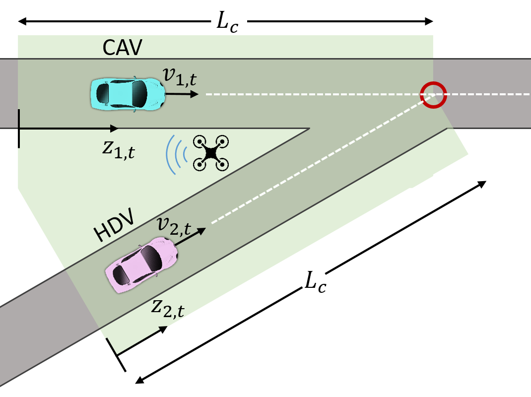
Figure 1: Control zone (green area) of our mixed traffic merging scenario and the conflict point (red circle).

In our formulation, the longitudinal positions of CAV–$1$ and HDV–$2$ are measured from the beginning of the control zone at any $t\in\mathbb{N}$, we denote them by $z_{1,t}\in\mathbb{R}_{\geq 0}$ and $z_{2,t}\in\mathbb{R}_{\geq 0}$, respectively. Let $v_{1,t}\in\mathbb{R}_{\geq 0}$ and $u_{1,t}\in\mathbb{R}$ be the speed and acceleration of CAV–$1$, $v_{2,t}\in\mathbb{R}_{\geq 0}$ and $u_{2,t}\in\mathbb{R}$ be the speed and acceleration of HDV–$2$ at time $t$. We collectively denote the position and speed of each vehicle $i=1,2$ as its state $x_{i,t}=(z_{i,t}\,,\,v_{i,t})$ at time $t$. Then, starting with the initial state $x_{1,0}$ and $x_{2,0}$ at $t=0$, the state of each vehicle evolves according to

$${x}_{1,t+1}=f_{1,t}({x}_{1,t},{u}_{1,t}),$$ (1)

$${x}_{2,t+1}=f_{2,t}({x}_{2,t},{u}_{2,t}).$$ (2)

In this paper, we consider that for all $t\in\mathbb{N}$ the dynamics of CAV–$1$ from (1) takes the form of the following double-integrator model

$$\begin{split}z_{1,t+1}&=z_{1,t}+\Delta Tv_{1,t}+\frac{1}{2}\Delta T^{2}u_{1,t},\\ v_{1,t+1}&=v_{1,t}+\Delta Tu_{1,t},\\ \end{split}$$ (3)

where $\Delta T\in\mathbb{R}_{>0}$ is the sampling time between two discrete timesteps. We consider the following state and control constraints for CAV–$1$

$$0\leq v_{\text{min}}\leq v_{1,t}\leq v_{\text{max}},\quad\text{and}\quad u_{\text{min}}\leq u_{1,t}\leq u_{\text{max}},$$ (4)

where $u_{\text{min}}$, $u_{\text{max}}\in\mathbb{R}$ are the minimum deceleration and maximum acceleration, respectively, and $v_{\text{min}}$, $v_{\text{max}}\in\mathbb{R}_{>0}$ are the minimum and maximum speed limits, respectively. Both CAV–$1$ and HDV–$2$ are restricted to only move in the forward direction, and hence, their speeds $v_{i,t}$ for $i=1,2$ are always non-negative. However, we do not impose an upper bound on the speed of HDV–$2$ that is known a priori because it can be violated by human driving behavior. In the next subsection, we formulate the control problem for CAV–$1$.

II-A Model Predictive Control Formulation

In this subsection, we formulate an MPC problem to control CAV–$1$ in the merging scenario given the system dynamics (3) and the state and control constraints (4). Let $H\in\mathbb{N}$ be the time length of the control horizon, $t\in\mathbb{N}$ be the current time step, and $\mathcal{I}_{t}=\{t,\dots,t+H-1\}$ be the set of all time steps in the control horizon originating at $t$. The objective of the MPC problem can be formed by a linear combination of three features: (i) minimizing the control input, (ii) minimizing the deviation from the maximum allowed speed to reduce the travel time, and (iii) a logarithmic penalty function corresponding to a collision avoidance constraint [9]. Thus, the objective function for CAV–$1$ at any time $k$ is given by the cost

$$\begin{multlined}l(x_{1,k+1},u_{1,k})=\omega_{1}u_{1,k}^{2}+\omega_{2}(v_{1,k+1}-v_{\text{max}})^{2}\\ -\omega_{3}\log\big{(}(z_{1,k+1}-z_{c}+\rho v_{1,k+1})^{2}\\ +(\hat{z}_{2,k+1}-z_{c}+\rho\hat{v}_{2,k+1})^{2}\big{)},\end{multlined}l(x_{1,k+1},u_{1,k})=\omega_{1}u_{1,k}^{2}+\omega_{2}(v_{1,k+1}-v_{\text{max}})^{2}\\ -\omega_{3}\log\big{(}(z_{1,k+1}-z_{c}+\rho v_{1,k+1})^{2}\\ +(\hat{z}_{2,k+1}-z_{c}+\rho\hat{v}_{2,k+1})^{2}\big{)},$$ (5)

where $\omega_{1}$, $\omega_{2}$, and $\omega_{3}$ are positive weights, $z_{c}$ is the position of the conflict point, and $\rho\in\mathbb{R}_{>0}$ is a parameter which accounts for the reaction delay of HDV–$2$. An increase in $\rho$ represents an increase in the conservatism of the objective by accounting for HDV–$2$ to have greater reaction delays. In (5), $\hat{z}_{2,k+1}$ and $\hat{v}_{2,k+1}$ denote the predicted future positions and speeds of HDV–$2$ at time step $k+1$. Then, the MPC problem for CAV–$1$ is formulated for each $t\in\mathbb{N}$ as

$$\begin{multlined}\underset{\{u_{1,k}\}_{k\in\mathcal{I}_{t}}}{\operatorname*{minimize}}\;\sum_{k\in\mathcal{I}_{t}}l({x}_{1,k+1},u_{1,k}),\end{multlined}\underset{\{u_{1,k}\}_{k\in\mathcal{I}_{t}}}{\operatorname*{minimize}}\;\sum_{k\in\mathcal{I}_{t}}l({x}_{1,k+1},u_{1,k}),$$ (6b)

$$\text{subject to: }\eqref{eq:integrator},\eqref{eq:bound}.$$ (6c)

We seek the control inputs $(u_{1,t},\dots,u_{1,t+H-1})$ to minimize (6) at each $t\in\mathbb{N}$ without prior knowledge of the dynamics of HDV–$2$ given in (2). Thus, CAV–$1$ must learn a model that can predict the future trajectory of HDV–$2$ required in the objective (5). To ensure that CAV–$1$ has access to the real-time data of HDV–$2$, in our framework, we impose the following assumption.

Assumption 1.

A coordinator, which we can consider that is a drone shown in Fig. 1, exists to collect real-time observations on the states and control actions of HDV–$2$ and transmit them to CAV–$1$ instantaneously. The coordinator can achieve this without any noise in either observation or communication.

Remark 1.

The future control actions and the trajectory for HDV–$2$ are not pre-determined for the horizon because (i) the dynamics of HDV–$2$ are unknown, and (ii) the impact of the state and actions of CAV–$1$ on the actions of HDV–$2$ is also unknown. Anticipating that HDV–$1$ would react in response to the control actions of CAV–$1$ [8], we model the joint dynamics of both CAV–$1$ and HDV–$2$ as an unknown partially observable Markov decision process (POMDP). Next, we use the framework of approximate information states for POMDPs to learn a model that predicts the trajectory of HDV–$2$ coupled with the actions of CAV–$1$.

III Learning Framework

III-A Preliminaries

In this subsection, we present the mathematical formulation of POMDPs and the framework of approximate information states from [18]. This formulation helps us lay the foundation to understand how we analyze our system with incomplete knowledge of underlying dynamics. Subsequently, we will use this framework in our merging scenario to learn a model to predict the future trajectory of HDV–$2$.

POMDP Fundamentals: We define a POMDP as a tuple $(\mathcal{X},\mathcal{U},\mathcal{Y},T,O,c,\gamma)$, where the set of feasible states is $\mathcal{X}$, the set of feasible control actions is $\mathcal{U}$, the set of feasible observations is $\mathcal{Y}$, the function $T:\mathcal{X}\times\mathcal{U}\times\mathcal{X}\to[0,1]$ yields the transition probability $T(x_{t},u_{t-1},x_{t+1})=p(x_{t+1}|x_{t},u_{t-1})$ for all $x_{t},x_{t+1}\in\mathcal{X}$ and $u_{t}\in\mathcal{U}$, the function $O:\mathcal{X}\times\mathcal{Y}\to[0,1]$ yields the observation probability $O({x}_{t+1},{y}_{t+1})=p({y}_{t+1}|{x}_{t+1})$ for all $x_{t+1}\in\mathcal{X}$ and $y_{t+1}\in\mathcal{Y}$, the function $c:\mathcal{X}\times\mathcal{U}\to\mathbb{R}$ yields the cost $c(x_{t},u_{t})$ for all $x_{t}\in\mathcal{X}$ and $u_{t}\in\mathcal{U}$, and $\gamma\in[0,1)$ is the discount factor. The history of observations and control actions up to a given time $t$ constitutes the memory defined as ${m}_{t}=({m}_{t-1},{y}_{t},{u}_{t-1})\in\mathcal{M}_{t}$.

Approximate Information State: An approximate information state is a compression of the data of our system stored in a memory which can be used to compute an approximately optimal control strategy for a POMDP using a dynamic programming decomposition. In the context of our problem, it has the important property that an approximate information state model can be learned purely from observation data without complete knowledge of underlying dynamics. Consider a measurable space $(\mathcal{X},\mathcal{B}(\mathcal{X}))$, where $\mathcal{B}(\mathcal{X})$ is the sigma algebra on $\mathcal{X}$. We denote an integral probability metric between any two probability distributions $\mu,\nu\in\Delta(\mathcal{X})$ by $d(\cdot,\cdot)$. Examples of such metrics are the total variation metric, Wasserstein metric, and maximum mean discrepancy metric. Then, for a POMDP with a horizon $T\in\mathbb{N}$, a time-invariant approximate information state model is defined by a tuple $(\mathcal{S},\hat{p},\hat{c},\sigma_{t}:t=0,\dots,T)$, where $\mathcal{S}$ is a Banach space of feasible information states, $\hat{p}:\mathcal{S}\times\mathcal{U}\to\Delta(\mathcal{S})$ is a Markovian probability kernel, $\hat{c}:\mathcal{S}\times\mathcal{U}\to\mathbb{R}$ is an approximate cost function, and $\sigma_{t}:\mathcal{M}_{t}\to\mathcal{S}$ is a memory compression function. This constitutes an $(\varepsilon,\delta)$-approximate model of the POMDP if there exist $\varepsilon,\delta\in\mathbb{R}_{>0}$ such that for all realizations of memory ${m}_{t}\in\mathcal{M}_{t}$ and realizations of control action ${u}_{t}\in\mathcal{U}$, the following properties hold:

(AP1) Sufficient to predict the cost $c_{t}=c({x}_{t},{u}_{t})$ approximately

$$\left|\mathbb{E}[c_{t}({x}_{t},{u}_{t})\,|\,{m}_{t},{u}_{t}]-\hat{c}(\sigma_{t}({m}_{t}),{u}_{t})\right|\leq\varepsilon.$$ (7)

(AP2a) The approximate information state evolves in a deterministic manner, i.e., there exists a measurable update function $\psi:\mathcal{S}\times\mathcal{Y}\times\mathcal{U}\to\mathcal{S}$ such that

$$\sigma_{t}({m}_{t})=\psi(\sigma_{t}({m}_{t-1}),{y}_{t},{u}_{t-1}).$$ (8)

(AP2b) Sufficient to approximately predict future observations, i.e., there exists a probability kernel $\hat{p}^{\text{y}}:\mathcal{S}\times\mathcal{U}\to\Delta(\mathcal{Y})$ such that for any Borel subset $B$ of $\mathcal{Y}$, the memory-based distribution $\mu_{t}(B)=p(y_{t+1}\in B|m_{t},u_{t})$ and the predicted distribution $\phi(B)=\hat{p}^{\text{y}}(y_{t+1}\in B|\sigma_{t}(m_{t}),u_{t})$ satisfy

$$d(\mu_{t},\phi)\leq\delta.$$ (9)

An $(\varepsilon,\delta)$-approximate information state model forms a perfectly observed Markov decision process with the state at each $t$ given by $s_{t}\in\mathcal{S}$. Thus, we can use it to compute an approximately optimal control strategy by formulating a dynamic programming decomposition of the problem. It has been established that such an approximate strategy has a bounded performance loss and that the performance improves linearly with a decrease in $\varepsilon$ and $\delta$ [18, Theorem 9]. This property implies that an approximate information state constitutes a principled compression of the memory, which can be learned by best enforcing $(\textbf{AP1})$ and $(\textbf{AP2b})$ while ensuring that $(\textbf{AP2a})$ is satisfied.

In light of these advantages, we adopt this framework in our CAV-HDV merging scenario to predict the trajectory of HDV–$1$ and, subsequently, compute a control strategy for CAV–$1$. In this framework, at each $t\in\mathbb{N}$, the state of CAV–$1$ is $x_{1,t}=(z_{1,t}\,,\,v_{1,t})$, the control action is $u_{1,t}$ and the observation received by CAV–$1$ is $y_{t}=(z_{1,t}\,,\,v_{1,t}\,,\,u_{1,t-1}\,,\,z_{2,t}\,,\,v_{2,t}\,,\,u_{2,t-1})$. We deploy an encoder-decoder neural network architecture to represent an approximate information state model which learns a representation of the unknown impact of CAV–$1$’s actions on the actions of HDV–$2$. This is illustrated in Fig. 2, where we denote the encoder by $\psi:\mathcal{S}\times\mathcal{Y}\times\mathcal{U}\to\mathcal{S}$ and the decoder by $\phi:\mathcal{S}\times\mathcal{U}\to\mathcal{Y}^{3}$, where $\mathcal{Y}\subset\mathbb{R}^{6}$. We seek to learn this approximate information state model purely from observation data. For this, we compare the distributions predicted by the decoder against data that constitutes sampled points from the ground truth. Next, we describe each component of our neural network architecture.

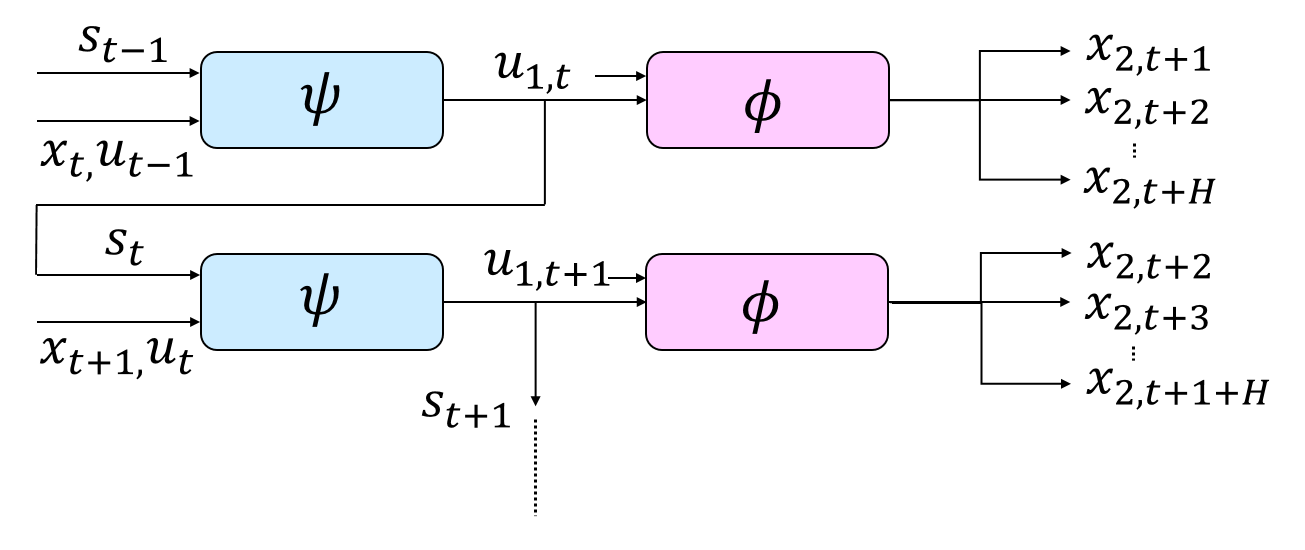
Figure 2: A visualization of the encoder-decoder architecture.

III-B Encoder

The encoder $\psi$ aims to learn a functional mapping which enforces $(\textbf{AP2a})$, i.e., its aim is to compress the history of observations into an approximate information state which can represent the CAV-HDV interactions. Thus, at each $t\in\mathbb{N}$, the output of the encoder is the approximate information state $s_{t}=\sigma_{t}(m_{t})$, where $m_{t}$ is the memory, and its input includes the previous approximate information state, latest observation, and previous control action given as a tuple $(s_{t-1},y_{t},u_{t-1})$. We illustrate this in Fig. 2. The encoder comprises of two fully connected layers followed by a recurrent neural network (RNN). The hidden state of the RNN at each $t\in\mathbb{N}$ is treated as the output of the encoder $s_{t}$. The linear layers are responsible for receiving the inputs $(y_{t},u_{t-1})$, and the RNN ensures that the encoder at time $t$ receives the previous approximate information state $s_{t-1}$ as an input too. Thus, the structure of the RNN ensures that the approximate information state is updated at each $t\in\mathbb{N}$ as

$$s_{t}=\psi(s_{t-1},y_{t},u_{t-1}),$$ (10)

where $\psi$ is a deterministic function and denotes the mapping generated by layers of neural networks within the encoder.

III-C Decoder

The decoder $\phi$ aims to learn a functional mapping which enforces $(\textbf{AP1})$ and $(\textbf{AP2b})$, i.e., its aim is to learn to predict distribution on future observations and the expected cost as a function of the approximate information state and the control action at any instance of time. In our implementation, the decoder $\phi$ comprises of three fully connected layers. At each $t\in\mathbb{N}$, the decoder takes as an input the approximate information state $s_{t}$ and control action $u_{1,t}$ of CAV–$1$. The decoder generates as an output a distribution of future states of HDV–$2$ over a horizon $\mathcal{I}_{t}$, $(x_{2,t+1},x_{2,t+2},\dots,x_{2,t+H})$, rather than just the next observation $y_{t+1}$. Thus, the output of the decoder is given by

$$\phi({s}_{t},{u}_{1,t})=\hat{p}^{\text{y}}({x}_{2,t+1},\dots,{x}_{2,t+H}~{}|~{}{s}_{t},{u}_{1,t}),$$ (11)

where $\hat{p}^{\text{y}}$ is the predicted probability distribution on the observations. Thus, in our architecture, the decoder aims to enforce $(\textbf{AP2b})$ not just for time $t+1$ as described in (9) but for the entire control horizon $\mathcal{I}_{t}$. This serves two purposes: (i) it allows for a planning depth across the control horizon $\mathcal{I}_{t}$ during the implementation of the MPC controller, and (ii) it focuses the output of the decoder on predicting the future states of HDV–$2$. We do not include an expected cost term in the output of the decoder because the cost (5) at each time is a deterministic function of the observations and predictions of CAV–$1$. Note that we can focus only on HDV–$2$ because the dynamics of CAV–$1$ are already known from (3) and need not be learned. Thus, if the decoder learns to best predict the trajectories, it automatically ensures both $(\textbf{AP1})$ and $(\textbf{AP2b})$.

III-D Training

In this subsection, we describe how we train both the encoder $\psi$ and the decoder $\phi$ by considering the left-hand side in (9) from (AP2b) as a training loss. Thus, the training loss measures the distance between a predicted probability distribution on observed future states and the underlying distribution on the ground truth using an integral probability metric. For this purpose, we use the distance-based maximum mean discrepancy (MMD) metric defined in [19, Proposition 32] to characterize the distance between two probability distributions.

Let the underlying distribution on the ground truth be denoted by $p$ and the predicted distribution of the decoder be $\hat{p}^{\text{y}}$. The training loss is then given by $d(\hat{p}^{\text{y}},p)^{2}$, where $d(\cdot,\cdot)$ is the MMD metric. From (11), note that the distribution $\hat{p}^{\text{y}}$ is parameterized by the weights of the encoder-decoder network. We consider that this is a multivariate normal distribution on the possible future realizations of the states $({x}_{2,t+1},\dots,{x}_{2,t+H})$ of HDV–$2$ over the horizon $\mathcal{I}_{t}$. Then, we fix the standard deviation of $\hat{p}^{\text{y}}$ to $1$ and consider that outputs of the decoder represent the mean value vector of the distribution. At each $t\in\mathbb{N}$, we have access to a sampled observation $({x}^{\text{ref}}_{2,t+1},\dots,{x}^{\text{ref}}_{2,t+H})$ from the underlying distribution $p$. To minimize the loss $d(\hat{p}^{\text{y}},p)^{2}$, we need to construct an unbiased estimator of the gradient of this training loss using only sampled points. From [19, Proposition 33], the gradient $\nabla d(\hat{p}^{\text{y}},p)^{2}$ can be estimated in an unbiased manner from the mean of $\hat{p}^{\text{y}}$ and sampled points from $p$ by the gradient of

$$({x}_{2,t+i}-2\cdot{x}^{ref}_{2,t+i})^{\top}x_{2,t+i}.$$ (12)

We use (12) as a surrogate loss for the training, which is computed using the predicted mean $({x}_{2,t+1},\dots,{x}_{2,t+H})$ and the sample from the ground truth $({x}^{\text{ref}}_{2,t+1},\dots,{x}^{\text{ref}}_{2,t+H})$.

IV Simulation and Results

IV-A Datasets

We train and validate the use of approximate information state models for three datasets that contain trajectories of HDVs in highway on-ramp merging scenarios. For the first dataset, we collect trajectory data from the NGSIM repository for I-80 [25]. Specifically, we extract the positions, velocities, and accelerations of the vehicle on the ramp as well as the two consecutive highway vehicles that it interacts with during merging. We use this data to validate the predictive ability of our approximate information state model for the trajectories of human-driven vehicles in real-life merging scenarios. The training details for specializing in the architecture from Section III to perform this task and the results are presented in Subsection IV-B.

Next, we use an inverse reinforcement learning (IRL) technique described in [26] to replicate human drivers in simulations and generate two datasets for the scenario presented in Section II. With the IRL technique, we assume that the control actions of an HDV can be represented by the minimizer of a feature-based objective function in which different driving styles are characterized by the weights of the features. By conducting and collecting data from simulations with different parameters for HDV’s model, we can capture a full spectrum of possible actions for a human driver, ranging from conservative to aggressive driving. This approach yields the second and third datasets used in the training and validation of approximate information state models in our subsequent exposition. In the second dataset, we consider that CAV–$1$ follows a safe control strategy proposed in [9] against different HDVs. This ensures that only $1$% of the situations included in the dataset demonstrate an unsafe merging scenario. In the third dataset, we consider that the control actions of both HDV–$2$ and CAV–$1$ are generated using the IRL technique with randomized weights. This simulates an exploratory control strategy for the CAV and does not include any consideration for safety during data generation. We use the second and third datasets to validate the performance of the MPC strategy presented in Subsection IV-D. This MPC approach utilizes the predictions of an approximate information state model trained individually on each dataset to generate control actions for CAV–$1$ against a variety of behaviors for HDV–$2$.

In the following subsections, we present the details for training an approximate information state model on each dataset and the validation of the trained models. Note that the encoder-decoder neural network architectures do not assume prior knowledge of the strategy or the model used to generate the data.

IV-B Network Architecture and Results for NGSIM

In this subsection, we train both an encoder and a decoder to cumulatively learn an approximate information state model for the first dataset collected from the NGSIM repository. Recall from Subsection IV-A that our dataset includes the trajectory information for the vehicle on the ramp and two consecutive highway vehicles that interact with it. Thus, at each instance of time, the encoder $\psi$ takes as input the most recent observation of each vehicle’s state and action, i.e., a $9$ dimensional input consisting of a $2$ dimensional observation of position and speed and $1$ dimensional action for each vehicle. The encoder comprises two fully connected layers of dimensions $(9,8)$ and $(8,16)$ each with a ReLU activation, followed by a recurrent gated unit (GRU) [27] layer with a hidden state of size $24$. We consider the hidden state to be the output of the encoder and treating it as the approximate information state at any instance of time. The approximate information state and the most recent actions of each vehicle are provided as input to the decoder $\phi$. The decoder comprises three fully connected layers with dimensions $(24+3,32),(32,64)$, and $(64,2)$, respectively, and with ReLU activation for the first two layers. The decoder is trained to predict the trajectory of the on-ramp vehicle for a horizon of $H=1$ time steps. A comparison of the predicted trajectories for three on-ramp vehicles with their actual trajectories is plotted in Fig. 3. Each column in this plot corresponds to a single vehicle, where the plots in the first row are a comparison of the position in the direction perpendicular to the highway (labeled as lateral position), and in the second row, we plot the position along the direction of the highway (labeled as longitudinal position). The approximate information state model performs well in predicting the longitudinal positions. At the same time, our model is capable of closely predicting the trajectory of the on-ramp vehicle along both the lateral and longitudinal axes. The root mean square error between the reference and predicted trajectories in the lateral positions are $0.35$ m for 3(a), $0.39$ m for 3(b), and $0.54$ m for 3(c), whereas it is $2.62$ m for 3(a), $1.92$ m for 3(b), and $1.73$ m for 3(c) in the longitudinal positions. These results validate the predictive capability of our approximate information state model for real-life merging scenarios involving human-driven vehicles.

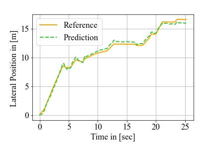
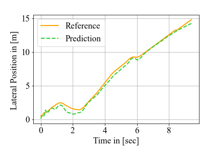
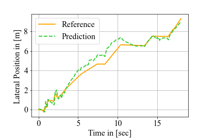
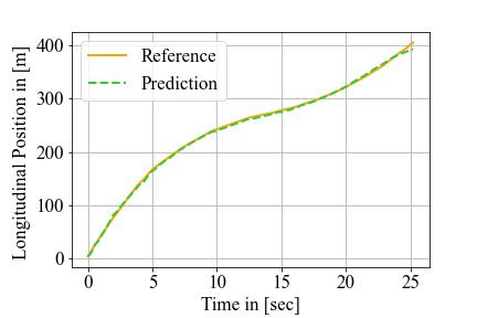
(a)

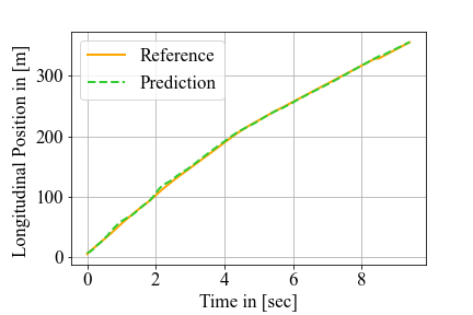
(b)

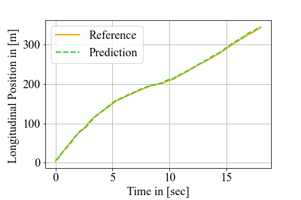
(c)

Figure 3: A collection of plots showing the results of trajectory prediction v/s the reference trajectory from the NGSIM dataset for three different cars (a), (b), and (c) merging from the ramp.

IV-C Network Architecture for IRL

In this subsection, we present the details of the encoder-decoder architecture used to learn approximate information state models for both datasets generated using IRL.

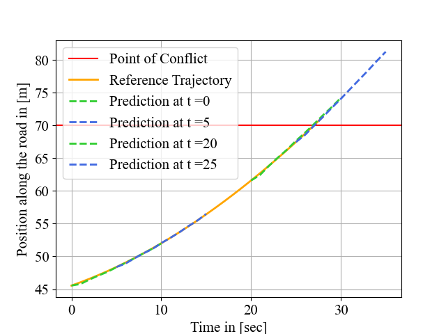
Figure 4: The results of trajectory prediction $v/s$ are the actual trajectory from the generated dataset.

The encoder and decoder follow the same underlying structure as the networks used in Subsection IV-B. Since we consider the scenario presented in Section II, we reduce the number of inputs and outputs in each layer compared to the previous networks. Note that we use identical networks across the generated datasets. At each instance of time, the encoder $\psi$ takes as input the most recent observation of the state and action of both CAV–$1$ and HDV–$2$, which is a $6$ dimensional input consisting of a $2$ dimensional observation of position and speed and $1$ dimensional action for each vehicle. The encoder structure is given by $(6,8),(8,16)$ with ReLU activation followed by a GRU with a hidden state of size $4$. Once again, we consider the hidden state to be the output of the encoder and treating it as the approximate information state at any instance of time. The approximate information state and the most recent action of CAV–$1$ is provided as input to the decoder $\phi$. The decoder comprises three fully connected layers of dimensions $(4+1,2),(2,4)$, and $(4,H)$, respectively, where H is the length of the horizon and a ReLU activation for the first two layers. We use the distance-based MMD described in (12) to train the encoder-decoder neural network architectures. We present the results of trajectory prediction in Fig. 4, where we compare the predicted trajectories at different time instances $t=0,5,20,25$ sec to the reference trajectory. The root mean square error between all predicted and reference trajectories is $0.17$ m. For these datasets, we set the length of the control zone $L_{c}=70$ m and we indicate the conflict point using a red horizontal line.

IV-D Iterative MPC Implementation

To solve the MPC problem and obtain the control input $u_{1,t}$ for CAV–$1$ at the current time step $t$, we utilize the encoder-decoder neural network to predict the human driving trajectory over the control horizon. Meanwhile, the decoder of the neural network also requires $u_{1,t}$ as the input to make the prediction. One can consider the encoder-decoder neural network directly as a constraint in the MPC problem. However, due to the complexity of the neural network model, the resulting MPC problem becomes computationally intractable. Therefore, we propose an iterative MPC implementation that sequentially computes the neural network prediction and solves the MPC problem. The iterative MPC implementation can be detailed in Algorithm 1. At each time step, we initialize $u_{1,t}^{(0)}=0$ and compute the prediction of the approximate information state by ${s}_{t}=\psi({s}_{t-1},{x}_{t},{u}_{t-1})$ where the inputs include the previous approximate information state ${s}_{t-1}$, current states ${x}_{t}$, and previous control inputs ${u}_{t-1}$. Next, at each iteration $j$ of the algorithm, we predict states and control actions of HDV–2 by ${y}_{t+1:t+H}^{(j)}=\phi({s}_{t},{u}_{1,t}^{(j-1)})$ that use the approximate information state ${s}_{t}$ and the control input ${u}_{1,t}^{(j-1)}$ of the MPC in the last iteration. Then we solve the MPC problem given the prediction of ${y}_{t+1:t+H}^{(j)}$ to obtain the new control inputs ${u}_{1,t}^{(j)}$. This procedure is repeated until a maximum number of iterations $j_{\mathrm{max}}$ is reached.

Algorithm 1 Iterative MPC Implementation

1:$t$, $H\in\mathbb{N}$, $j_{\mathrm{max}}\in\mathbb{N}$, $u_{1,t}^{(0)}=0$

2:Predict the approximate information state by ${s}_{t}=\psi({s}_{t-1},{x}_{t},{u}_{t-1})$

3:for $j=1,2,\dots,j_{\mathrm{max}}$ do

4:     Predict states and control actions of HDV–$2$ by ${y}_{t+1:t+H}^{(j)}=\phi({s}_{t},{u}_{1,t}^{(j-1)})$

5:     Solve (6) to obtain ${u}_{1,t:t+H-1}^{(j)}$

6:return $u_{1,t}^{(j_{\mathrm{max}})}$

IV-E Simulation Results

We conducted simulations in Python programming language in which CasADi [28] and the built-in IPOPT solver [29] are used for formulating and solving the MPC problem, respectively. The parameters of MPC were chosen as: ${\Delta T=$0.2\text{\,}\mathrm{s}$}$, ${H=10}$, ${v_{\mathrm{min}}=$0.0\text{\,}\mathrm{m}\mathrm{/}\mathrm{s}$}$, ${v_{\mathrm{max}}=$14.0\text{\,}\mathrm{m}\mathrm{/}\mathrm{s}$}$, ${u_{\mathrm{min}}=$-3.0\text{\,}\mathrm{m}\mathrm{/}\mathrm{s}^{2}$}$, ${u_{\mathrm{max}}=$2.0\text{\,}\mathrm{m}\mathrm{/}\mathrm{s}^{2}$}$, ${\omega_{1}=1.0}$, ${\omega_{2}=10.0}$, ${\omega_{3}=10^{3}}$, ${\rho=$1.0\text{\,}\mathrm{s}$}$. Recall that we simulate human driving behavior by using an IRL-based model with different weights to validate the control method with different driving styles.

Figures 5 and 6 show the trajectories, speeds, and control inputs of CAV–$1$ and HDV–$2$ in two simulations with two human driving styles, i.e., an aggressive and a conservative human driver. As shown from the figures, in both simulations, safe distance is guaranteed, but CAV–$1$ has different merging maneuvers depending on the behavior of HDV–$2$. If the human driver accelerates to cross first, then CAV–$1$ slows down to yield, while if the human driver is more conservative, CAV–$1$ finds it safe to cross before HDV–$2$.

TABLE I: Comparison between models trained using safe and exploratory strategy data.

Reaction Time Delay $(\rho)$	Safe	Exploratory
0.6	4984 (99.6%)	4578 (91.5%)
0.8	4996 (99.9%)	4793 (95.8%)
1.0	5000 (100%)	4971 (99.4%)

To evaluate the performance of the MPC with two learned prediction models, we conduct 5000 simulations with different initial conditions of the vehicles and different IRL models for HDV–$2$ and compare the level of safety under three different values for $\rho$. Recall from Subsection II-A that CAV–$1$’s conservatism increases with $\rho$. Hence, we observe that the number of unsafe situations decreases with an increase in $\rho$. The results are indicated in Table I and show that MPC with the model trained using the safe-strategy dataset achieves a higher level of safety compared to the model trained using the exploratory-strategy dataset. We believe that this might be due to the model for the exploratory dataset requiring further training.

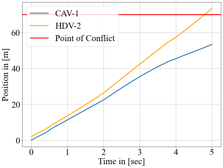
(a)

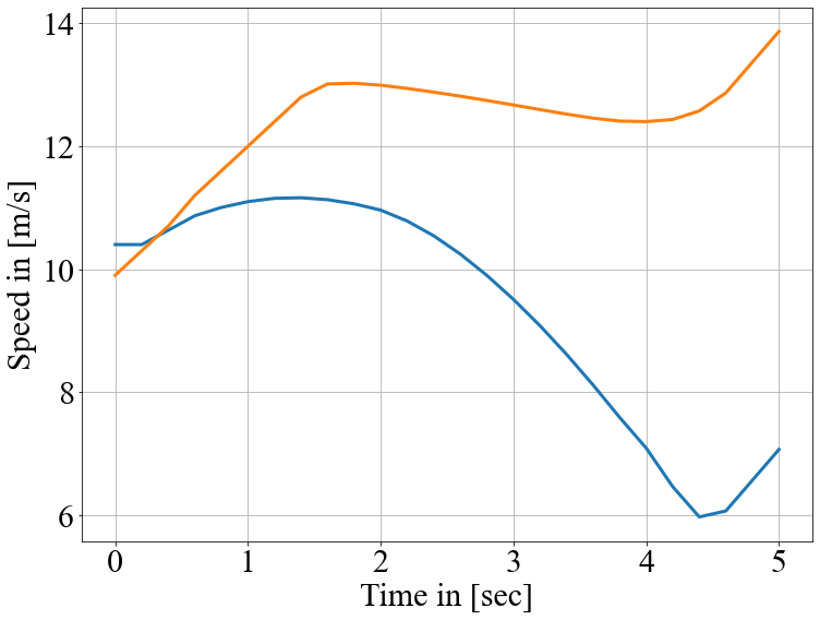
(b)

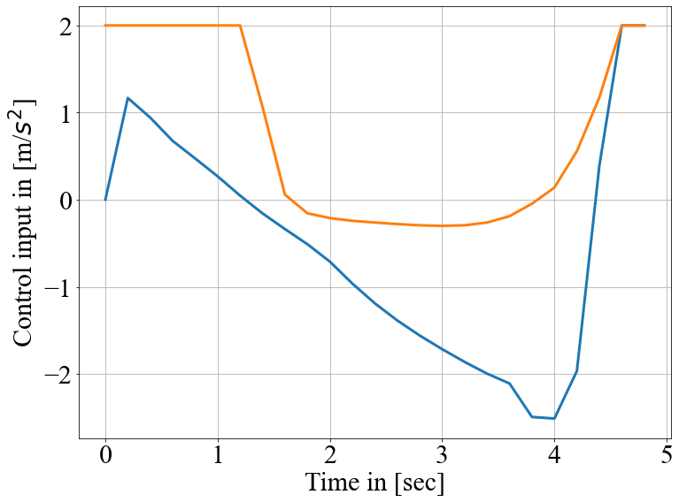
(c)

Figure 5: Trajectories, speeds, and distances of the vehicles in the simulation with an aggressive human driver.

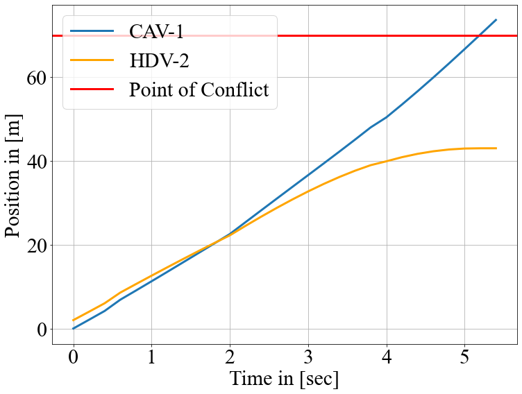
(a)

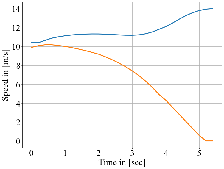
(b)

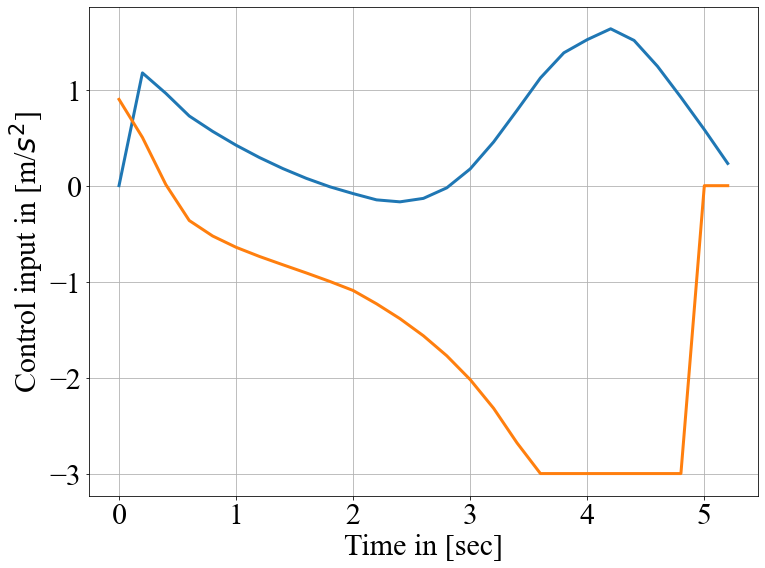
(c)

Figure 6: Trajectories, speeds, and distances of the vehicles in the simulation with a conservative human driver.

V Concluding Remarks

In this paper, we presented an approach to learn an approximate information state model of CAV-HDV interactions for a CAV to maneuver safely during highway merging. We validated the capability of our approximate information state model by training with and predicting real-life merging scenarios involving human-driven vehicles for the NGSIM repository. Then, we showed that using data generated from an IRL model for a mixed traffic scenario with a CAV and an HDV, an approximate information state model can be learned to predict future trajectories of the HDV. We proposed an iterative MPC algorithm to generate control actions for the CAV utilizing these predictions and showed using numerical simulations that they are safe against a spectrum of driving behaviors of the HDV. Future research should focus on (i) extending the framework for continuous-time control, (ii) considering a more diverse range of scenarios with multiple lanes, multiple cars, roundabouts, and intersections, and (iii) investigating the practical effectiveness of the a proposed approach using an experimental testbed [30].

References

- [1] L. Zhao and A. A. Malikopoulos, “Enhanced mobility with connectivity and automation: A review of shared autonomous vehicle systems,” IEEE Intelligent Transportation Systems Magazine, vol. 14, no. 1, pp. 87–102, 2022.
- [2] A. A. Malikopoulos, L. E. Beaver, and I. V. Chremos, “Optimal time trajectory and coordination for connected and automated vehicles,” Automatica, vol. 125, no. 109469, 2021.
- [3] W. Xiao and C. G. Cassandras, “Decentralized optimal merging control for Connected and Automated Vehicles with safety constraint guarantees,” Automatica, vol. 123, p. 109333, 2021.
- [4] B. Chalaki and A. A. Malikopoulos, “A barrier-certified optimal coordination framework for connected and automated vehicles,” in Proceedings of the 61th IEEE Conference on Decision and Control (CDC), pp. 2264–2269, 2022.
- [5] W. Gao, A. Odekunle, Y. Chen, and Z. Jiang, “Predictive cruise control of connected and autonomous vehicles via reinforcement learning,” IET Control Theory & Applications, vol. 13, pp. 2849–2855, Nov. 2019.
- [6] K. Liu, N. Li, H. E. Tseng, I. Kolmanovsky, A. Girard, and D. Filev, “Cooperation-Aware Decision Making for Autonomous Vehicles in Merge Scenarios,” in 2021 60th IEEE Conference on Decision and Control (CDC), pp. 5006–5012, IEEE, 2021.
- [7] R. Chandra and D. Manocha, “Gameplan: Game-theoretic multi-agent planning with human drivers at intersections, roundabouts, and merging,” IEEE Robotics and Automation Letters, vol. 7, no. 2, pp. 2676–2683, 2022.
- [8] V.-A. Le and A. A. Malikopoulos, “A Cooperative Optimal Control Framework for Connected and Automated Vehicles in Mixed Traffic Using Social Value Orientation,” in 2022 61th IEEE Conference on Decision and Control (CDC), pp. 6272–6277, 2022.
- [9] V.-A. Le and A. A. Malikopoulos, “Optimal Weight Adaptation of Model Predictive Control for Connected and Automated Vehicles in Mixed Traffic with Bayesian Optimization,” in Proceedings of 2023 American Control Conference (ACC), 2023 (to appear).
- [10] F. Altché and A. de La Fortelle, “An lstm network for highway trajectory prediction,” in 2017 IEEE 20th international conference on intelligent transportation systems (ITSC), pp. 353–359, IEEE, 2017.
- [11] S. H. Park, B. Kim, C. M. Kang, C. C. Chung, and J. W. Choi, “Sequence-to-sequence prediction of vehicle trajectory via lstm encoder-decoder architecture,” in 2018 IEEE intelligent vehicles symposium (IV), pp. 1672–1678, IEEE, 2018.
- [12] N. Deo and M. M. Trivedi, “Multi-modal trajectory prediction of surrounding vehicles with maneuver based lstms,” in 2018 IEEE intelligent vehicles symposium (IV), pp. 1179–1184, IEEE, 2018.
- [13] N. Deo and M. M. Trivedi, “Convolutional social pooling for vehicle trajectory prediction,” in Proceedings of the IEEE conference on computer vision and pattern recognition workshops, pp. 1468–1476, 2018.
- [14] B. Kim, C. M. Kang, J. Kim, S. H. Lee, C. C. Chung, and J. W. Choi, “Probabilistic vehicle trajectory prediction over occupancy grid map via recurrent neural network,” in 2017 IEEE 20th International Conference on Intelligent Transportation Systems (ITSC), pp. 399–404, IEEE, 2017.
- [15] Z. el abidine Kherroubi, S. Aknine, and R. Bacha, “Novel decision-making strategy for connected and autonomous vehicles in highway on-ramp merging,” IEEE Transactions on Intelligent Transportation Systems, vol. 23, no. 8, pp. 12490–12502, 2021.
- [16] J. Guo, S. Cheng, and Y. Liu, “Merging and diverging impact on mixed traffic of regular and autonomous vehicles,” IEEE Transactions on Intelligent Transportation Systems, vol. 22, no. 3, pp. 1639–1649, 2020.
- [17] A. A. Malikopoulos, “Separation of learning and control for cyber-physical systems,” Automatica, vol. 151, no. 110912, 2023.
- [18] J. Subramanian and A. Mahajan, “Approximate information state for partially observed systems,” in 2019 IEEE 58th Conference on Decision and Control (CDC), pp. 1629–1636, IEEE, 2019.
- [19] J. Subramanian, A. Sinha, R. Seraj, and A. Mahajan, “Approximate information state for approximate planning and reinforcement learning in partially observed systems,” Journal of Machine Learning Research, vol. 23, no. 12, pp. 1–83, 2022.
- [20] L. Yang, K. Zhang, A. Amice, Y. Li, and R. Tedrake, “Discrete approximate information states in partially observable environments,” in 2022 American Control Conference (ACC), pp. 1406–1413, IEEE, 2022.
- [21] M. Fatemi, T. W. Killian, J. Subramanian, and M. Ghassemi, “Medical dead-ends and learning to identify high-risk states and treatments,” Advances in Neural Information Processing Systems, vol. 34, pp. 4856–4870, 2021.
- [22] A. Dave, N. Venkatesh, and A. A. Malikopoulos, “Approximate information states for worst-case control of uncertain systems,” in Proceedings of the 61th IEEE Conference on Decision and Control (CDC), pp. 4945–4950, 2022.
- [23] A. Dave, N. Venkatesh, and A. A. Malikopoulos, “Approximate Information States for Worst-Case Control and Learning in Uncertain Systems,” arXiv:2301.05089 (in review), 2023.
- [24] M. Treiber and A. Kesting, “Traffic flow dynamics,” Traffic Flow Dynamics: Data, Models and Simulation, Springer-Verlag Berlin Heidelberg, pp. 983–1000, 2013.
- [25] U. S. D. of Transportation Federal Highway Administration, “Next generation simulation (ngsim) vehicle trajectories and supporting data,” 2016.
- [26] M. Kuderer, S. Gulati, and W. Burgard, “Learning driving styles for autonomous vehicles from demonstration,” in 2015 IEEE International Conference on Robotics and Automation (ICRA), pp. 2641–2646, IEEE, 2015.
- [27] K. Cho, B. Van Merriënboer, D. Bahdanau, and Y. Bengio, “On the properties of neural machine translation: Encoder-decoder approaches,” arXiv preprint arXiv:1409.1259, 2014.
- [28] J. A. Andersson, J. Gillis, G. Horn, J. B. Rawlings, and M. Diehl, “CasADi: a software framework for nonlinear optimization and optimal control,” Mathematical Programming Computation, vol. 11, no. 1, pp. 1–36, 2019.
- [29] A. Wächter and L. T. Biegler, “On the implementation of an interior-point filter line-search algorithm for large-scale nonlinear programming,” Mathematical programming, vol. 106, no. 1, pp. 25–57, 2006.
- [30] B. Chalaki, L. E. Beaver, A. I. Mahbub, H. Bang, and A. A. Malikopoulos, “A research and educational robotic testbed for real-time control of emerging mobility systems: From theory to scaled experiments [applications of control],” IEEE Control Systems Magazine, vol. 42, no. 6, pp. 20–34, 2022.