On the Sample Complexity of the Linear Quadratic Gaussian Regulator

Abstract

In this paper we provide direct data-driven expressions for the Linear Quadratic Regulator (LQR), the Kalman filter, and the Linear Quadratic Gaussian (LQG) controller using a finite dataset of noisy input, state, and output trajectories. We show that our data-driven expressions are consistent, since they converge as the number of experimental trajectories increases, we characterize their convergence rate, and we quantify their error as a function of the system and data properties. These results complement the body of literature on data-driven control and finite-sample analysis, and they provide new ways to solve canonical control and estimation problems that do not assume, nor require the estimation of, a model of the system and noise and do not rely on solving implicit equations.

I Introduction

Consider the discrete-time, linear, time-invariant system

$$x(t+1) =Ax(t)+Bu(t)+w(t),$$ (1)

$$y(t) =Cx(t)+v(t),\qquad t\geq 0,$$

where $x(t)\in{}^{n}$ denotes the state, $u(t)\in{}^{m}$ the control input, $y(t)\in{}^{p}$ the measured output, $w(t)$ and $v(t)$ the process and measurement noise at time $t$. The LQG control problem asks for the input that minimizes the cost function

$$\lim_{T\rightarrow\infty}\mathbb{E}\left[\frac{1}{T}\Big{(}\sum_{t=0}^{T-1}x(t)^{\mathsf{T}}Q_{x}x(t)+u(t)^{\mathsf{T}}R_{u}u(t)\Big{)}\right],$$ (2)

where $Q_{x}\succeq 0$, $R_{u}\succ 0$ are weight matrices and $T$ is the control horizon. With the standard assumptions that

• the process and measurement noise sequences and the initial state are independent at all times and satisfy $w(t)\!\sim\!\mathcal{N}(0,Q_{w})$, $v(t)\!\sim\!\mathcal{N}(0,R_{v})$, and $x(0)\!\sim\!\mathcal{N}(0,\Sigma_{0})$, with $Q_{w}\succeq 0$, $R_{v}\succ 0$, and $\Sigma_{0}\succ 0$;

• the pairs $(A,B)$ and $(A,Q_{w}^{\frac{1}{2}})$ are controllable, and the pairs $(A,C)$ and $(A,Q_{x}^{\frac{1}{2}})$ are observable;

the input that solves the LQG problem can obtained by concatenating the Kalman filter for (1) with the (static) controller that solves the LQR problem for (1) with weight matrices $Q_{x}$ and $R_{u}$ [1]. That is,

$$u^{*}(t)={K}_{\textup{LQR}}{x}_{\textup{KF}}(t),$$ (3)

where ${x}_{\textup{KF}}(t)$ is the Kalman estimate of the state $x(t)$. The classic, model-based computation of the LQR gain and Kalman filter in (3) requires the complete knowledge of the system (1), including the noise statistics. Motivated by the recent successes of data-driven and machine-learning methods, we seek here a solution to the LQG problem that relies only on a (finite) dataset of experimental data, without the need to estimate the system dynamics and noise statistics.

Related work. Data-driven methods for system analysis and control have flourished in the last years and are revolutionizing the field [2]. The methods developed in this paper fall in the category of direct data-driven methods [3], where controls are obtained directly from data bypassing the classic system identification step [4]. In line with earlier work and differently from optimization-based approaches [5, 6], we pursue here closed-form data-driven expressions, which are typically computationally advantageous [7], are transparent, and can reveal novel insights into the problems [8].

This paper focuses on data-driven LQG control, while most of the literature on data-driven control has focused on the LQR problem with noiseless data [9, 10, 11]. Recent work [12] has studied the design of data-driven controllers from noisy data [13, 14], the design of data-driven Kalman filters [15], imitation-based LQG control design [16], and some versions of the output-weighted LQG control problem [17, 18]. Compared to [18], in particular, this paper does not assume perfect knowledge of the Markov parameters or any part of the system dynamics and noise, and it does not estimate them to solve the state-weighted LQG problem. To the best of our knowledge, this paper contains the first direct, closed-form data-driven solution to the state-weighted LQG problem, with finite-sample performance guarantees.

The recent literature on the analysis of the sample complexity of estimation and control problems is also relevant to this work. In particular, [19, 20] follow an indirect approach, where sample complexity bounds are derived for the identification of the system dynamics and such errors are propagated towards the design of LQR and LQG controllers. Differently from this paper, this analysis is valid only for stable systems and output-weighted LQG costs. Bounds on the performance of the learned LQG controller are also derived in [21] assuming a sufficiently small error in the system identification step [22, 23, 24, 25], and in [26] where the optimal LQR is learned in a model-free setting using gradient methods. Although this paper makes use of similar technical tools, the approach pursued here is direct and does not rely on the identification of the system matrices, nor on optimization algorithms to design or tune robust controllers. Further, this paper considers the canonical LQG setting, rather than the noisy LQR problem or the output-weighted LQG problem with noisy controls, and it provides closed-form expressions for the optimal controllers rather than their performance.

Contributions of the paper. The main contributions of this paper is the characterization of direct data-driven formulas for the LQR gain, Kalman filter, and LQG gain using a dataset of trajectories of the input, state, and output of the system (1). Importantly, since the experimental data is noisy and the system dynamics and noise statistics are unknown, we show that our formulas are consistent, as they converge to the true expressions when the amount of experimental data increases. Additionally, we characterize the convergence rate of our expressions, as well as their error when the data is of finite size. Finally, we provide illustrative examples and remarks to highlight how the properties of the system and of the experimental data affect the accuracy of our formulas.

Organization of the paper. The remainder of the paper is organized as follows. Section II formalizes our problem setting and contains some preliminary results. Section III contains our main results and examples, and Section IV concludes the paper. Finally, all proofs are in the Appendix.

Notation. A Gaussian random variable $x$ with mean $\mu$ and covariance $\Sigma$ is denoted as $x\sim\mathcal{N}(\mu,\Sigma)$. The $n\times n$ identity matrix is denoted by $I_{n}$, and the $n\times m$ zero matrix is denoted by $0_{n\times m}$. The expectation operator is denoted by $\mathbb{E}[\cdot]$. The trace of a square matrix $A$ is denoted by $\mathrm{tr}\left[A\right]$. A positive definite (semidefinite) matrix $A$ is denoted as $A\succ 0$ ($A\succeq 0$). The Kronecker product is denoted by $\otimes$, and the vectorization operator is denoted by vec($\cdot$). The left (right) pseudo inverse of a tall (fat) matrix $A$ is denoted by $A^{\dagger}$. A block-diagonal matrix with block matrices $A$ and $B$ is denoted by $\mathrm{blkdiag}(A,B)$. The smallest (largest) singular value of a matrix $A$ is denoted by $\sigma_{\text{min}}(A)$ ($\sigma_{\text{max}}(A)$).

II Problem formulation and preliminary results

In this work we aim to compute the LQG inputs in a data-driven setting where datasets from offline experiments are available but the system matrices and noise statistics are unknown. In particular, we have access to the following data:

$$U\!=\!\begin{bmatrix}u^{1}\!\!\!&\!\!\cdots\!\!&\!\!\!u^{N}\end{bmatrix}\!,~{}X\!=\!\begin{bmatrix}x^{1}\!\!\!&\!\!\cdots\!\!&\!\!\!x^{N}\end{bmatrix}\!,~{}Y\!=\!\begin{bmatrix}y^{1}\!\!\!&\!\!\cdots\!\!&\!\!\!y^{N}\end{bmatrix}\!,$$ (4)

where $x^{i}$ and $y^{i}$ are the $i$-th state and output trajectories of (1) generated by the input $u^{i}$. That is, for $i\in\{1,\dots,N\}$,

$$u^{i} =\begin{bmatrix}u^{i}(0)\\ \vdots\\ u^{i}(T-1)\end{bmatrix},x^{i}=\begin{bmatrix}x^{i}(0)\\ \vdots\\ x^{i}(T)\end{bmatrix},y^{i}=\begin{bmatrix}y^{i}(0)\\ \vdots\\ y^{i}(T)\end{bmatrix},$$

where $T$ is the horizon of the control experiments. We make the following assumption on the experimental inputs.

Assumption II.1

(Experimental inputs) The inputs in (4) are independent and identically distributed, that is, $u^{i}(t)\sim\mathcal{N}(0,\Sigma_{u})$, with $\Sigma_{u}\succ 0$, for all $i\in\{1,\dots,N\}$ and times. $\square$

In our analysis we will make use of an equivalent characterization of the LQG inputs derived in [27, Theorem 2.1], which shows that these inputs can also be computed as

$$u^{*}(t+n)={K}_{\textup{LQG}}\begin{bmatrix}u^{*}(t)\\ \vdots\\ u^{*}(t+n-1)\\ y^{*}(t+1)\\ \vdots\\ y^{*}(t+n)\end{bmatrix},$$ (5)

where the static gain ${K}_{\textup{LQG}}$ depends on the system and noise matrices, and $y^{*}$ is the output of (1) with input $u^{*}$.

Remark 1

(State vs output measurements) We assume here that the state of the system (1) can be directly measured. This assumption is easily satisfied in certain lab experiments, where additional sensors (e.g., a motion capture system for robotic applications) can be deployed during the design stage to measure the system state and collect training data. Further, state measurements are necessary to solve the state-weighted LQG problem, since the state weight matrix $Q_{x}$ uses specific coordinates that cannot be inferred from output measurements only [28], but they can be substituted with input and output measurements for different versions of the LQG problem. See also [27] for a reformulation of the LQG problem that uses only input and output measurements. $\square$

III Data-driven formulas for LQG control

In this section we derive our main results, that is, direct data-driven formulas for the LQR controller, the Kalman filter, and the LQG controller using the data (4). Additionally, we show that these formulas are consistent, i.e., they converge to the true model-based expressions as the data grows, and we finally quantify their error when the data is finite.

We start by introducing some additional notation. Let

$$X_{t}=\begin{bmatrix}x^{1}(t)^{\mathsf{T}}&\cdots&x^{N}(t)^{\mathsf{T}}\end{bmatrix}^{\mathsf{T}},$$ (6)

and, given input and state trajectories ${u}_{\textup{v}}\in{}^{mT}$ and ${x}_{\textup{v}}\in{}^{nT}$, let ${u}_{\textup{m}}\in{}^{m\times T}$ and ${x}_{\textup{m}}\in{}^{n\times T}$ be the matrices obtained by reorganizing the inputs and states in the vectors ${u}_{\textup{v}}$ and ${x}_{\textup{v}}$ in chronological order. The next result characterizes the LQR gain from data.

Theorem III.1

(Data-driven LQR gain) Let $x_{0}\in{}^{n}$ and

$$\begin{bmatrix}{u}_{\textup{v}}\\ {x}_{\textup{v}}\end{bmatrix}=\begin{bmatrix}H\\ M\end{bmatrix}P^{-1/2}\left(\begin{bmatrix}I_{n}\!\!&\!\!0_{n\times mT}\end{bmatrix}P^{-1/2}\right)^{\dagger}x_{0},$$ (7)

where

$$\begin{split}H&=\begin{bmatrix}0_{mT\times n}\!\!&\!\!I_{mT}\end{bmatrix},M=X\begin{bmatrix}X_{0}\\ U\end{bmatrix}^{\dagger},\text{ and }\\ P&=M^{\mathsf{T}}\left(I_{T+1}\!\otimes\!Q_{x}\right)M+\mathrm{blkdiag}\left(0_{n\times n},I_{T}\!\otimes\!R_{u}\right).\end{split}$$ (8)

Let ${x}_{\textup{v}}^{*}\in{}^{nT}$ be the trajectory of (1) with initial state $x_{0}$, control input $u^{*}(t)={K}_{\textup{LQR}}x(t)$, and $w(t)=0$ at all times. Then, the data-driven estimate $K_{\text{LQR}}^{\text{D}}={u}_{\textup{m}}{x}_{\textup{m}}^{{\dagger}}$ of $K_{\text{LQR}}$

$$\|{K}_{\textup{LQR}}-K_{\text{LQR}}^{\text{D}} \|_{2}\leq\frac{1}{{\sigma}_{\textup{min}}({x}_{\textup{m}}^{*})\left(1-\kappa({x}_{\textup{m}}^{*})\right)}\left(\frac{c_{1}}{\sqrt{N}}+c_{2}\rho^{T}\right)\!,$$

for sufficiently large $N$ and probability at least $1-6\delta$, where

$$\kappa({x}_{\textup{m}}^{*})=\frac{{\sigma}_{\textup{max}}({x}_{\textup{m}}-{x}_{\textup{m}}^{*})}{{\sigma}_{\textup{min}}({x}_{\textup{m}}^{*})},$$

where the constants $c_{1}$ and $c_{2}$ are independent of $N$ and are defined in (32), $\rho<1$, and $\delta\in[0,1/6]$. $\square$

A proof of Theorem III.1 is postponed to Appendix B. Some comments are in order. First, Theorem III.1 provides a direct, data-driven way to estimate the LQR gain from noisy data, namely, $K_{\text{LQR}}^{\text{D}}$, and characterizes the error between the true and the estimated gains. Such error vanishes as the number ($N$) and length ($T$) of the experimental trajectories grow. Further, the term $\kappa({x}_{\textup{m}}^{*})$ also vanishes as the number of experimental trajectories increases (see Theorem B.3). Second, the vectors ${u}_{\textup{v}}$ and ${x}_{\textup{v}}$ contain an estimate of the optimal input and state trajectories that minimize the LQR cost with matrices $Q_{x}$ and $R_{u}$ for the system (1) with initial state $x_{0}$ and without process noise. Notably, these trajectories are estimated using the noisy dataset (4). Thus, this result extends the analysis in [7]. Third, Theorem III.1 is valid when $N$ is sufficiently large. In particular, $N$ needs to be at least large enough to satisfy $\kappa({x}_{\textup{m}}^{*})<1$ (see Appendix B for other conditions on $N$). Also, the result holds with probability $1-6\delta$, and the specific choice of $\delta$ affects the magnitude of the constant $c_{1}$. Fourth and finally, although formulas with similar convergence rates for the estimation of the LQR exist [19, 21], Theorem III.1 provides an alternative, direct, closed-form expression of the gain, as opposed to indirect and optimization-based approaches. This will allow us to estimate the LQG controller.

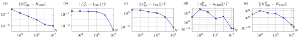
Figure 1: This figure shows the error between the data-driven and the model-based gains as a function of the size of the data in (4) for the setting described in Example 1, 2, and 3. Panel (a) shows the error between the model-based LQR gain and the data-based LQR gain obtained from Theorem III.1 as a function of $N$ for the setting described in Example 1. Panel (b) shows the error between the model-based Kalman filter and the data-based Kalman filter obtained from Theorem III.2, and panel (c) shows the error between the corresponding state estimates as a function of $N$ for the setting in Example 2. Panel (d) shows the error between the model-based LQG input generated by (3) and the data-based LQG input generated by (11) as a function of $N$. Panel (e) shows the error between the model-based LQG gain in (5) and the data-based LQG gain obtained from Theorem III.3 as a function of $N$ for the setting in Example 3. We observe that all the quantities in the plots decrease as the number of trajectories, $N$, increases, which agrees with our theoretical results.

Example 1

(Estimating the LQR gain from noisy data) Consider System (1) with

$$A=\begin{bmatrix}0.7&1.2\\ 0&0.4\end{bmatrix},\quad B=\begin{bmatrix}0\\ 1\end{bmatrix},\quad C=\begin{bmatrix}1&0\end{bmatrix},$$

$Q_{x}\!\!=\!\!5I_{2}$, $Q_{w}\!\!=\!\!2I_{2}$, $R_{u}\!=\!R_{v}\!=\!\Sigma_{u}\!\!=\!\!1$, and $\Sigma_{0}\!=\!I_{2}$. We collect open-loop trajectories as in (4) generated by inputs satisfying Assumption II.1 with horizon $T\!\!=\!\!50$. The model-based LQR gain is $K_{\text{LQR}}\!\!=\!\![0.241\;\;0.788]$. We use Theorem III.1 to compute the data-driven LQR gain, $K_{\text{LQR}}^{\text{D}}$ for different values of $N$. Fig. 1(a) shows the error $\|K_{\text{LQR}}^{\text{D}}\!\!-\!K_{\text{LQR}}\|$ as a function of the number of trajectories.  $\square$

We now focus on estimating the Kalman filter from noisy data with unknown system dynamics and noise statistics.

Theorem III.2

(Data-driven Kalman filter) Let $U_{t}$ and $Y_{t}$ be the submatrices of $U$ and $Y$ in (4) obtained by selecting only the inputs and outputs up to time $t$. Let

$$L_{t}^{\text{D}}=X_{t}\begin{bmatrix}U_{t-1}\\ Y_{t}\end{bmatrix}^{\dagger},$$ (9)

where $X_{t}$ is as in (6). Then, for every $t\in[0,T]$,

$$\left\|{x}_{\textup{KF}}(t)-L_{t}^{\text{D}}\begin{bmatrix}[c]u_{0}^{t-1}\\ y_{0}^{t}\end{bmatrix}\right\|_{2}\leq\frac{c_{3}}{\sqrt{N}}{\left\|\begin{bmatrix}u_{0}^{t-1}\\ y_{0}^{t}\end{bmatrix}\right\|}_{2},$$ (10)

with probability at least $1-2\delta$, where $u_{0}^{t}$ and $y_{0}^{t}$ are the vectors of inputs and outputs of (1), respectively, from time $0$ up to time $t$, $c_{3}$ is a constant independent of $N$ as defined in (38), and $\delta\in[0,1/2]$.  $\square$

A proof of Theorem III.2 is postponed to Appendix C. Theorem III.2 provides a way to construct an approximate Kalman filter using a finite set of experimental data, without knowing the system dynamics and the statistics of the noise. As can be seen from (10), the error vanishes with rate $1/\sqrt{N}$ as the number of experimental data grows, showing the consistency of the data-driven Kalman filter expressions (9).

Example 2

(Estimating the Kalman filter from noisy data) Following the setting introduced in Example 1, we use Theorem III.2 to obtain the data-driven Kalman filter, $L_{\text{KF}}^{\text{D}}$, and the corresponding data-driven state estimate, $x_{\text{KF}}^{\text{D}}$. Fig. 1(b) and 1(c) show the errors $\|L_{\text{KF}}^{\text{D}}\!\!-\!L_{\text{KF}}\|$ and $\|x_{\text{KF}}^{\text{D}}\!\!-\!x_{\text{KF}}\|$.  $\square$

Theorems III.1 and III.2 allow us to compute the LQG inputs from time $0$ up to time $T$. In particular, recalling the structure of the LQG inputs due to the separation principle [1],

$$u_{\text{dLQG}}(t)=K_{\text{LQR}}^{\text{D}}\underbrace{L_{t}^{\text{D}}\begin{bmatrix}u_{\text{dLQG}}(0)\\ \vdots\\ u_{\text{dLQG}}(t-1)\\ y_{\text{dLQG}}(0)\\ \vdots\\ y_{\text{dLQG}}(t)\end{bmatrix}}_{x_{\text{KF}}^{\text{D}}(t)},$$ (11)

where $x_{\text{KF}}^{\text{D}}$ is the state estimate obtained using our data-driven scheme. Fig. 1(d) shows how these data-driven inputs compare to the model-based LQG inputs as a function of the amount of data. As expected, the performance gap between the data-driven and the model-based schemes shrinks as the amount of data increases. We next provide an estimate of the LQG gain (5), which allows us to compute LQG inputs beyond the horizon $T$ of the experimental trajectories. We start by collecting $M\geq n+nm+np$ closed-loop input-output trajectories of system (1) driven by the LQG inputs generated from (11). In particular,

$${U}_{\text{dLQG}}\!=\!\!\begin{bmatrix}u_{\text{dLQG}}^{1}\!\!\!&\!\!\cdots\!\!&\!\!\!u_{\text{dLQG}}^{M}\end{bmatrix}\!,~{}Y_{\text{dLQG}}\!=\!\begin{bmatrix}y_{\text{dLQG}}^{1}\!\!\!&\!\!\cdots\!\!&\!\!\!y_{\text{dLQG}}^{M}\end{bmatrix}\!,$$ (12)

where $y_{\text{dLQG}}^{i}$ is the $i$-th output trajectory of (1) generated by the LQG input $u_{\text{dLQG}}^{i}$ in (11). That is, for $i\in\{1,\dots,M\}$,

$$u_{\text{dLQG}}^{i} \!=\!\!\begin{bmatrix}u_{\text{dLQG}}^{i}(0)\\ \vdots\\ u_{\text{dLQG}}^{i}(T\!-\!1)\end{bmatrix}\!\!,\quad y_{\text{dLQG}}^{i}\!=\!\!\begin{bmatrix}y_{\text{dLQG}}^{i}(0)\\ \vdots\\ y_{\text{dLQG}}^{i}(T)\end{bmatrix}\!.$$

Theorem III.3

(Data-driven LQG gain) Let $U^{n}_{\text{dLQG}}$ and $Y_{\text{dLQG}}^{n}$ be the submatrices of $U_{\text{dLQG}}$ and $Y_{\text{dLQG}}$ in (12) obtained by selecting only the inputs from time $T-n$ up to time $T-1$ and the outputs from time $T-n+1$ up to time $T$, respectively. Define the data-driven LQG gain as

$$K_{\text{LQG}}^{\text{D}}= K_{\text{LQR}}^{\text{D}}L_{t}^{\text{D}}\underbrace{\begin{bmatrix}U_{\text{dLQG}}\\ Y_{\text{dLQG}}\end{bmatrix}\begin{bmatrix}U^{n}_{\text{dLQG}}\\ Y^{n}_{\text{dLQG}}\end{bmatrix}^{\dagger}}_{c_{4}},$$

Then, the data-driven estimate of the LQG gain satisfies

$$\|K_{\text{LQG}}-K_{\text{LQG}}^{\text{D}}\|_{2}\leq\|c_{4}\|_{2}\left(\frac{c_{5}+c_{6}\rho^{T}}{\sqrt{N}}+c_{7}\rho^{T}\right),$$ (13)

for sufficiently large $T$ and $N$ and probability at least $1-8\delta$, where the constants $c_{5}$, $c_{6}$, and $c_{7}$ are independent of $N$ and are defined in (41), $\rho<1$, and $\delta\in[0,1/8]$.   $\square$

We postpone the proof of Theorem III.3 to Appendix D. Theorem (III.3) provides a direct data-driven expression of the LQG gain that converges with polynomial rate as the experimental data increases. To the best of our knowledge, this result is the first of its kind, and it provides a new way to compute the LQG controller using offline experimental data and a finite number of online experiments, without knowing or identifying the system and noise matrices.

Example 3

(Estimating the LQG gain from noisy data) Following the setting introduced in Example 1 and Example 2, we use Theorem III.3 to obtain the data-driven LQG gain, $K_{\text{LQG}}^{\text{D}}$. Fig. 1(e) shows the error $\|K_{\text{LQG}}^{\text{D}}\!\!-\!K_{\text{LQG}}\|$ as a function of the number of trajectories, $N$.  $\square$

IV Conclusion

In this paper we derive direct data-driven expressions for the LQR gain, Kalman filter, and LQG controller using a dataset of input, state, output trajectories. We show the convergence of these expressions as the size of the dataset increases, we characterize their convergence rate, and we quantify the error incurred when using a dataset of finite size. Our expressions are direct, as they do not use a model of the system nor require the estimation of a model, and provide new insights into the solution of canonical control and estimation problems. Directions of future research include the direct data-driven solution to $\mathcal{H}_{2}$ and $\mathcal{H}_{\infty}$ problems, as well as the extension of the results to accomodate for incomplete, heterogeneous and, possibly, corrupted datasets.

Appendix

A Technical lemmas

Lemma A.1

(Product of Gaussian matrices [19, Lemma 1]) Let $A\!=\![a_{1},\cdots\!,a_{N}]$ and $B\!=\![b_{1},\cdots\!,b_{N}]$, where $\left.a_{i}\in\mathbb{R}^{n}\right.$ and $b_{i}\in\mathbb{R}^{m}$ are independent random vectors with $a_{i}\sim\mathcal{N}(0,\Sigma_{a})$ and $b_{i}\sim\mathcal{N}(0,\Sigma_{b})$ for $i=1,\cdots,N$. Let $\delta\in[0,1]$ and $N\geq 2(n+m)\log{(1/\delta)}$. Then, with probability at least $1-\delta$

$${\|AB^{\mathsf{T}}\|}_{2}\leq 4{\|\Sigma_{a}\|}_{2}^{1/2}{\|\Sigma_{b}\|}_{2}^{1/2}\sqrt{N(n+m)\log{(9/\delta)}}.$$

$\square$

Lemma A.2

(Singular values of a Gaussian matrix) Let $\delta\in[0,1]$, and let $A\in\mathbb{R}^{n\times N}$ be a random matrix with independent entries distributed as $\mathcal{N}(0,1)$. Then, for $N\geq 8n+16\log{(1/\delta)}$, each of the following inequalities hold with probability probability at least $1-\delta$

$${\sigma}_{\textup{min}}(A)\geq\sqrt{N}/2,\qquad{\sigma}_{\textup{max}}(A)\leq 3\sqrt{N}/2,$$

where ${\sigma}_{\textup{min}}$ (${\sigma}_{\textup{max}}$) is the smallest (largest) singular value. $\square$

Proof:

For notational convenience, we use ${\sigma}_{\textup{min}}$, ${\sigma}_{\textup{max}}$, and $\delta^{\prime}$ to denote ${\sigma}_{\textup{min}}(A)$, ${\sigma}_{\textup{max}}(A)$, and $2\log{(1/\delta)}$, respectively. From [29, Corollary 5.35], we have each of the following inequalities holds with probability at least $1-\delta$

$${\sigma}_{\textup{min}}\geq\sqrt{N}-\sqrt{n}-\sqrt{\delta^{\prime}},\quad{\sigma}_{\textup{max}}\!\leq\!\sqrt{N}\!+\sqrt{n}+\sqrt{\delta^{\prime}}.$$ (14)

Assume that $N\geq 8n+8\delta^{\prime}$. Then,

$$\sqrt{N}/2\geq\sqrt{n}+\sqrt{\delta^{\prime}},$$ (15)

where we have used the inequality $2(a^{2}+b^{2})\geq(a+b)^{2}$. The proof follows by substituting (15) into (14). ∎

B Proof of Theorem III.1

Let ${u}_{\textup{v}}^{*}\in{}^{mT}$ and ${x}_{\textup{v}}^{*}\in{}^{nT}$ be the optimal LQR trajectories of (1) from the initial state $x_{0}$. Then, ${K}_{\textup{LQR}}={u}_{\textup{m}}^{*}{x}_{\textup{m}}^{*^{\dagger}}$ asymptotically as the control horizon $T$ grows. Further, from [7, 30], the trajectories ${u}_{\textup{v}}^{*}$ and ${x}_{\textup{v}}^{*}$ can be obtained using (7) when the state data is not corrupted by the process noise. Let ${X}_{\textup{clean}}$ be such data, that is, the state trajectories of (1) with inputs $U$ and noise $w(t)=0$ at all times. Notice that in our setting $X$ is different from ${X}_{\textup{clean}}$ since the process noise is nonzero when the data is collected. Because of this deviation in the data, the vectors ${u}_{\textup{v}}$ and ${x}_{\textup{v}}$ in (7) are a perturbed version of the optimal trajectories ${u}_{\textup{v}}^{*}$ and ${x}_{\textup{v}}^{*}$. Accordingly, $K_{\text{LQR}}^{\text{D}}={u}_{\textup{m}}{x}_{\textup{m}}^{{\dagger}}$ is a perturbed version of ${K}_{\textup{LQR}}$. To quantify the deviation between $K_{\text{LQR}}^{\text{D}}$ and ${K}_{\textup{LQR}}$, we quantify (i) the deviation in the data induced by the process noise, (ii) the sensitivity of the map (7) that generates LQR trajectories, and (iii) how the induced errors propagate to compute $K_{\text{LQR}}^{\text{D}}$.

(i) Data deviation induced by the process noise. Note that

$$X=\underbrace{\left[\begin{array}[]{c;{2pt/2pt}c}O&F_u\end{array}\right]}_{F}\underbrace{\left[\begin{array}[]{c}X_{0}\\ \hdashline[2pt/2pt]U\end{array}\right]}_{\overline{U}}+F_{w}W,$$ (19)

where $W\in\mathbb{R}^{nT\times N}$ is a matrix that contains the corresponding $N$ process noise realizations of horizon $T-1$, and

Note that ${X}_{\textup{clean}}=F\mkern 1.5mu\overline{\mkern-1.5muU\mkern-1.5mu}\mkern 1.5mu$. Let the data matrices in (4) and (6) be partitioned as

$$U=\begin{bmatrix}{U}_{\textup{d}}&{U}_{\textup{n}}\end{bmatrix},X=\begin{bmatrix}{X}_{\textup{d}}&{X}_{\textup{n}}\end{bmatrix},X_{0}=\begin{bmatrix}X_{0,\text{d}}&X_{0,\text{n}}\end{bmatrix},$$ (20)

where ${U}_{\textup{d}}$, ${X}_{\textup{d}}$, and $X_{0,\text{d}}$ contain the first $N_{\text{d}}\geq mT+n$ columns of $U$, $X$, and $X_{0}$, respectively, and let $\mkern 1.5mu\overline{\mkern-1.5muU\mkern-1.5mu}\mkern 1.5mu=[{\mkern 1.5mu\overline{\mkern-1.5muU\mkern-1.5mu}\mkern 1.5mu}_{\textup{d}},{\mkern 1.5mu\overline{\mkern-1.5muU\mkern-1.5mu}\mkern 1.5mu}_{\textup{n}}]$ be partitioned similarly. For notational convenience, we define $Q_{T}=(I_{T+1}\otimes Q_{x})$ and $R_{T}=\mathrm{blkdiag}(0_{n\times n},I_{T}\otimes R_{u})$. Noting that $\mkern 1.5mu\overline{\mkern-1.5muU\mkern-1.5mu}\mkern 1.5mu_{\text{d}}{\mkern 1.5mu\overline{\mkern-1.5muU\mkern-1.5mu}\mkern 1.5mu_{\text{d}}}^{\dagger}=I_{n+mT}$, we rewrite ${u}_{\textup{v}}$ in (7) as

$${u}_{\textup{v}}=HP^{-1/2}\left(\begin{bmatrix}I_{n}\!\!&\!\!0_{n\times mT}\end{bmatrix}P^{-1/2}\right)^{\dagger}x_{0},$$ (21)

with

$$P \!=\!\left({\widetilde{X}}_{\textup{c}}{\mkern 1.5mu\overline{\mkern-1.5muU\mkern-1.5mu}\mkern 1.5mu}_{\textup{d}}^{\dagger}\right)^{\mathsf{T}}\!Q_{T}\!\left({\widetilde{X}}_{\textup{c}}{\mkern 1.5mu\overline{\mkern-1.5muU\mkern-1.5mu}\mkern 1.5mu}_{\textup{d}}^{\dagger}\right)\!+\!R_{T},~{}\text{and}~{}{\widetilde{X}}_{\textup{c}}=\!X\mkern 1.5mu\overline{\mkern-1.5muU\mkern-1.5mu}\mkern 1.5mu^{\dagger}{\mkern 1.5mu\overline{\mkern-1.5muU\mkern-1.5mu}\mkern 1.5mu}_{\textup{d}}.$$ (22)

Further, let

$${X}_{\textup{c}}={X}_{\textup{clean}}\mkern 1.5mu\overline{\mkern-1.5muU\mkern-1.5mu}\mkern 1.5mu^{\dagger}{\mkern 1.5mu\overline{\mkern-1.5muU\mkern-1.5mu}\mkern 1.5mu}_{\textup{d}}\quad\text{and}\quad\Delta_{X}={\widetilde{X}}_{\textup{c}}-{X}_{\textup{c}}.$$ (23)

Notice that if the process noise, $W$, is zero, then $\Delta_{X}=0$ and ${\widetilde{X}}_{\textup{c}}={X}_{\textup{c}}$ and, from (7), ${u}_{\textup{v}}={u}_{\textup{v}}^{*}$ and ${x}_{\textup{v}}={x}_{\textup{v}}^{*}$. Thus, we use $\Delta_{X}$ as a proxy for the deviation between $X$ and ${X}_{\textup{clean}}$, which is induced by the process noise, $F_{w}W$. The next Lemma provides a non-asymptotic upper bound to ${\|\Delta_{X}\|}_{2}$.

Lemma B.1

(Non-asymptotic bound on ${\|\Delta_{X}\|}_{2}$) Let $\Delta_{X}$ be as in (23), and let $\delta\in[0,1/3]$. Assume that $\left.N>\max{\{N_{1},N_{\text{d}}\}}\right.$, with $N_{1}=2\left((n+m)T+n\right)\log{\left(1/\delta\right)}$ and $N_{\text{d}}\geq 8(mT+n)+16\log{\left(1/\delta\right)}$. Then, with probability at least $1-3\delta$,

$${\|\Delta_{X}\|}_{2}\leq d_{1}\sqrt{\frac{N_{\text{d}}\left((n+m)T+n\right)\log{\left(9/\delta\right)}}{N}},$$ (24)

where $d_{1}=24\|F_{w}\|_{2}\|\mkern 1.5mu\overline{\mkern-1.5muQ\mkern-1.5mu}\mkern 1.5mu_{w}\|_{2}^{1/2}$ and $\mkern 1.5mu\overline{\mkern-1.5muQ\mkern-1.5mu}\mkern 1.5mu_{w}=I_{T}\otimes Q_{w}$. $\square$

Proof:

Let $\mkern 1.5mu\overline{\mkern-1.5muU\mkern-1.5mu}\mkern 1.5mu=\Sigma_{\mkern 1.5mu\overline{\mkern-1.5muu\mkern-1.5mu}\mkern 1.5mu}^{1/2}Z$ and ${\mkern 1.5mu\overline{\mkern-1.5muU\mkern-1.5mu}\mkern 1.5mu}_{\textup{d}}=\Sigma_{\mkern 1.5mu\overline{\mkern-1.5muu\mkern-1.5mu}\mkern 1.5mu}^{1/2}{Z}_{\textup{d}}$, where $\Sigma_{\overline{u}}=\mathrm{blkdiag}{\left(\Sigma_{0},I_{T}\otimes\Sigma_{u}\right)}$, $Z\in\mathbb{R}^{n+mT\times N}$ is a random matrix whose columns are independent copies of $\mathcal{N}\sim(0,I_{n+mT})$, and ${Z}_{\textup{d}}$ contains the first $N_{\text{d}}$ columns of $Z$. From (22), (23),

$${\|\Delta_{X}\|}_{2} \!=\!{\|F_{w}\!W\mkern 1.5mu\overline{\mkern-1.5muU\mkern-1.5mu}\mkern 1.5mu^{\mathsf{T}}\!(\mkern 1.5mu\overline{\mkern-1.5muU\mkern-1.5mu}\mkern 1.5mu\mkern 1.5mu\overline{\mkern-1.5muU\mkern-1.5mu}\mkern 1.5mu^{\mathsf{T}})^{-1}{\mkern 1.5mu\overline{\mkern-1.5muU\mkern-1.5mu}\mkern 1.5mu}_{\textup{d}}\|}_{2}\!=\!{\|F_{w}\!W\!Z^{\mathsf{T}}\!(ZZ^{\mathsf{T}})^{-1}{Z}_{\textup{d}}\|}_{2}$$

$$\leq{\|F_{w}\|}_{2}{\|WZ^{\mathsf{T}}\|}_{2}{\|(ZZ^{\mathsf{T}})^{-1}\|}_{2}{\|{Z}_{\textup{d}}\|}_{2}.$$

The proof follows by using Lemma A.1 to bound ${\|WZ^{\mathsf{T}}\|}_{2}$, Lemma A.2 to bound ${\|(ZZ^{\mathsf{T}})^{-1}\|}_{2}$ and ${\|{Z}_{\textup{d}}\|}_{2}$, and using the union bound to compute the probability. ∎

(ii) Sensitivity of map (7) w.r.t. $\Delta_{X}$. We focus our analysis on the map $\left.f:\mathbb{R}^{n(T+1)N_{\text{d}}}\times\mathbb{R}^{(n+mT)N_{\text{d}}}\rightarrow\mathbb{R}^{n+mT}\right.$ that generates ${u}_{\textup{v}}$ as in (21). Then, ${u}_{\textup{v}}^{*}=f(\text{vec}{({X}_{\textup{c}})},\text{vec}{({\mkern 1.5mu\overline{\mkern-1.5muU\mkern-1.5mu}\mkern 1.5mu}_{\textup{d}})})$. Since $f$ is Fréchet-differentiable with respect to $\text{vec}{({X}_{\textup{c}})}$ [30, 31], we can write its first-order Taylor-series expansion as

$$\begin{split}f(\text{vec}{({\widetilde{X}}_{\textup{c}})},\text{vec}{({\mkern 1.5mu\overline{\mkern-1.5muU\mkern-1.5mu}\mkern 1.5mu}_{\textup{d}})})&\!=\!f(\text{vec}{({X}_{\textup{c}})},\text{vec}{({\mkern 1.5mu\overline{\mkern-1.5muU\mkern-1.5mu}\mkern 1.5mu}_{\textup{d}})})\\ +\nabla f_{X}&\left(\text{vec}{({X}_{\textup{c}})},\text{vec}{({\mkern 1.5mu\overline{\mkern-1.5muU\mkern-1.5mu}\mkern 1.5mu}_{\textup{d}})}\right)\!\text{vec}{(\Delta_{X})},\end{split}$$ (25)

where $\nabla f_{X}$ is the Jacobian matrix of $f(\text{vec}{({X}_{\textup{c}})},\text{vec}{({\mkern 1.5mu\overline{\mkern-1.5muU\mkern-1.5mu}\mkern 1.5mu}_{\textup{d}})})$ with respect to $\text{vec}{({X}_{\textup{c}})}$. We quantify the sensitivity of the map (21) to the change in ${X}_{\textup{c}}$ by $\nabla f_{X}$ (large values of $\nabla f_{X}$ implies higher sensitivity). Next, we derive an upper bound on ${\|\nabla f_{X}\|}_{2}$, and upper bounds on ${\|{u}_{\textup{v}}-{u}_{\textup{v}}^{*}\|}_{2}$ and ${\|{x}_{\textup{v}}-{x}_{\textup{v}}^{*}\|}_{2}$ using the first-order approximation in (25).

Lemma B.2

(Non-asymptotic bound on $\|\nabla f_{X}\|_{2})$ Let ${\mkern 1.5mu\overline{\mkern-1.5muU\mkern-1.5mu}\mkern 1.5mu}_{\textup{d}}$, ${X}_{\textup{c}}$, and $\nabla f_{X}\left(\text{vec}{({X}_{\textup{c}})},\text{vec}{({\mkern 1.5mu\overline{\mkern-1.5muU\mkern-1.5mu}\mkern 1.5mu}_{\textup{d}})}\right)$ be as in (23) and (25). Also, let $\delta\in[0,1]$ and assume that $N_{\text{d}}\geq 8(n+mT)+16\log{(1/\delta)}$. Then, with probability at least $1-\delta$,

$$\left\|\nabla f_{X}\left(\text{vec}{({X}_{\textup{c}})},\text{vec}{({\mkern 1.5mu\overline{\mkern-1.5muU\mkern-1.5mu}\mkern 1.5mu}_{\textup{d}})}\right)\right\|_{2}\leq 4d_{2}\sqrt{\frac{n(T+1)}{N_{\text{d}}}},$$ (26)

where $d_{2}>0$ is independent of $N_{\text{d}}$. $\square$

Proof:

The proof can be adapted from the proof of [30, Lemma IV.4], then using Lemma A.2 and $\|\cdot\|_{2}\leq\|\cdot\|_{\mathrm{F}}$. ∎

Theorem B.3

(Non-asymptotic bound on the deviation of the LQR trajectories) Let ${u}_{\textup{v}}$ and ${x}_{\textup{v}}$ be as in (7) and ${u}_{\textup{v}}^{*}$ and ${x}_{\textup{v}}^{*}$ be the optimal LQR trajectories of length $T$ of (1) from the initial state $x_{0}$. Let $\delta\in[0,1/6]$ and assume that $N\geq\max{\left\{N_{1},N_{2},N_{3}\right\}}$, with $N_{1}=2\left((n+m)T+n\right)\log{\left(1/\delta\right)}$, $N_{2}=8(mT+n)+16\log{\left(1/\delta\right)}$, and $N_{3}=((n+m)T+n)\log{\left(9/\delta\right)}$. Then, with probability at least $1-4\delta$,

$$\begin{split}\|{u}_{\textup{v}}-{u}_{\textup{v}}^{*}\|_{2}&\leq d_{3}\sqrt{\frac{\left((n+m)T+n\right)\log{(9/\delta)}}{N}}.\end{split}$$ (27)

Further, with probability at least $1-6\delta$,

$$\begin{split}\|{x}_{\textup{v}}-{x}_{\textup{v}}^{*}\|_{2}\leq&d_{4}\sqrt{\frac{\left((n+m)T+n\right)\log{(9/\delta)}}{N}},\end{split}$$ (28)

with

$$d_{3} =4d_{1}d_{2}\sqrt{qn(T+1)},$$

$$d_{4} ={\|F\|}_{2}d_{3}+16{\|F_{w}\|}_{2}{\|\Sigma_{\mkern 1.5mu\overline{\mkern-1.5muu\mkern-1.5mu}\mkern 1.5mu}^{-1/2}\|}_{2}{\|\mkern 1.5mu\overline{\mkern-1.5muQ\mkern-1.5mu}\mkern 1.5mu_{w}\|}_{2}^{1/2}\left({\|{\mkern 1.5mu\overline{\mkern-1.5muu\mkern-1.5mu}\mkern 1.5mu}_{\textup{v}}^{*}\|}_{2}+d_{3}\right),$$

where $d_{1}$, $F$, and $F_{w}$ are as in (24) and (19), respectively, $d_{2}>0$ is independent of $N$, $q=\operatorname{Rank}{(\Delta_{X})}\leq n(T+1)$, ${\mkern 1.5mu\overline{\mkern-1.5muu\mkern-1.5mu}\mkern 1.5mu}_{\textup{v}}^{*}=[x_{0}^{\mathsf{T}},{{u}_{\textup{v}}^{*}}^{\mathsf{T}}]^{\mathsf{T}}$, and $\mkern 1.5mu\overline{\mkern-1.5muQ\mkern-1.5mu}\mkern 1.5mu_{w}$ and $\Sigma_{\overline{u}}$ are as in Lemma B.1. $\square$

Proof:

Inequality (27) follows from (25) by using Lemma B.1, Lemma B.2, and ${\|\text{vec}{(\Delta_{X})}\|}_{2}={\|\Delta_{X}\|}_{\mathrm{F}}\leq\sqrt{q}{\|\Delta_{X}\|}_{2}$, with $q=\operatorname{Rank}{(\Delta_{X})}$. Next, we derive (28). For notational convenience, we use $\Delta_{u}$ and $\Delta_{x}$ to denote ${u}_{\textup{v}}-{u}_{\textup{v}}^{*}$ and ${x}_{\textup{v}}-{x}_{\textup{v}}^{*}$, respectively. From (7), we can write

$${\|\Delta_{x}\|}_{2} =\left\|{\widetilde{X}}_{\textup{c}}{\mkern 1.5mu\overline{\mkern-1.5muU\mkern-1.5mu}\mkern 1.5mu}_{\textup{d}}^{\dagger}\begin{bmatrix}x_{0}\\ {u}_{\textup{v}}\end{bmatrix}-{X}_{\textup{c}}{\mkern 1.5mu\overline{\mkern-1.5muU\mkern-1.5mu}\mkern 1.5mu}_{\textup{d}}^{\dagger}\begin{bmatrix}x_{0}\\ {u}_{\textup{v}}^{*}\end{bmatrix}\right\|_{2}$$ (29)

$$=\left\|{X}_{\textup{c}}{\mkern 1.5mu\overline{\mkern-1.5muU\mkern-1.5mu}\mkern 1.5mu}_{\textup{d}}^{\dagger}\begin{bmatrix}0\\ \Delta_{u}\end{bmatrix}+\Delta_{X}{\mkern 1.5mu\overline{\mkern-1.5muU\mkern-1.5mu}\mkern 1.5mu}_{\textup{d}}^{\dagger}\begin{bmatrix}x_{0}\\ {u}_{\textup{v}}^{*}\end{bmatrix}+\Delta_{X}{\mkern 1.5mu\overline{\mkern-1.5muU\mkern-1.5mu}\mkern 1.5mu}_{\textup{d}}^{\dagger}\begin{bmatrix}0\\ \Delta_{u}\end{bmatrix}\right\|_{2}$$

$$\leq\|{X}_{\textup{c}} {\mkern 1.5mu\overline{\mkern-1.5muU\mkern-1.5mu}\mkern 1.5mu}_{\textup{d}}^{\dagger}\|_{2}\|\Delta_{u}\|_{2}+\|\Delta_{X}{\mkern 1.5mu\overline{\mkern-1.5muU\mkern-1.5mu}\mkern 1.5mu}_{\textup{d}}^{\dagger}\|_{2}\|{\mkern 1.5mu\overline{\mkern-1.5muu\mkern-1.5mu}\mkern 1.5mu}_{\textup{v}}^{*}\|_{2}+\|\Delta_{X}{\mkern 1.5mu\overline{\mkern-1.5muU\mkern-1.5mu}\mkern 1.5mu}_{\textup{d}}^{\dagger}\|_{2}\|\Delta_{u}\|_{2}.$$

Note that ${\mkern 1.5mu\overline{\mkern-1.5muU\mkern-1.5mu}\mkern 1.5mu}_{\textup{d}}{\mkern 1.5mu\overline{\mkern-1.5muU\mkern-1.5mu}\mkern 1.5mu}_{\textup{d}}^{\dagger}=I_{n+mT}$. Then we have

$${\|{X}_{\textup{c}}{\mkern 1.5mu\overline{\mkern-1.5muU\mkern-1.5mu}\mkern 1.5mu}_{\textup{d}}^{\dagger}\|}_{2} =\|{X}_{\textup{clean}}\mkern 1.5mu\overline{\mkern-1.5muU\mkern-1.5mu}\mkern 1.5mu^{\dagger}\|_{2}=\|F\|_{2},$$

$${\|\Delta_{X}{\mkern 1.5mu\overline{\mkern-1.5muU\mkern-1.5mu}\mkern 1.5mu}_{\textup{d}}^{\dagger}\|}_{2} \!=\!\!\|(X\!-\!{X}_{\textup{clean}})\mkern 1.5mu\overline{\mkern-1.5muU\mkern-1.5mu}\mkern 1.5mu^{\dagger}\|_{2}=\|F_{w}W\mkern 1.5mu\overline{\mkern-1.5muU\mkern-1.5mu}\mkern 1.5mu^{\dagger}\|_{2}$$

$$\!\leq\!\|F_{w}\|_{2}\|W\mkern 1.5mu\overline{\mkern-1.5muU\mkern-1.5mu}\mkern 1.5mu^{\mathsf{T}}\|_{2}\|(\mkern 1.5mu\overline{\mkern-1.5muU\mkern-1.5mu}\mkern 1.5mu\mkern 1.5mu\overline{\mkern-1.5muU\mkern-1.5mu}\mkern 1.5mu^{\mathsf{T}})^{-1}\|_{2},$$

Inequality (28) follows from (29) by using (27), Lemma A.1, and Lemma A.2 to bound $\|\Delta_{u}\|_{2}$, $\|W\mkern 1.5mu\overline{\mkern-1.5muU\mkern-1.5mu}\mkern 1.5mu^{\mathsf{T}}\|_{2}$, and $\|(\mkern 1.5mu\overline{\mkern-1.5muU\mkern-1.5mu}\mkern 1.5mu\mkern 1.5mu\overline{\mkern-1.5muU\mkern-1.5mu}\mkern 1.5mu^{\mathsf{T}})^{-1}\|_{2}$, respectively, and noting that for $N\geq N_{3}$ we have $\frac{\delta^{\prime}}{N}\leq\sqrt{\frac{\delta^{\prime}}{N}}$, with $\delta^{\prime}=\left((n+m)T+n\right)\log{(9/\delta)}$. The probabilities follow from the union bound. ∎

(iii) Error between ${K}_{\textup{LQR}}$ and $K_{\text{LQR}}^{\text{D}}$. We are now ready to conclude the proof of Theorem III.1. Notice that

$${u}_{\textup{m}}^{*}={K}_{\textup{LQR}}{x}_{\textup{m}}^{*},\text{ and }{u}_{\textup{m}}^{*}+\delta_{u}={K}_{\textup{LQR}}^{\text{D}}\left({x}_{\textup{m}}^{*}+\delta_{x}\right),$$ (30)

where $\delta_{u}={u}_{\textup{m}}-{u}_{\textup{m}}^{*}$ and $\delta_{x}={x}_{\textup{m}}-{x}_{\textup{m}}^{*}$. Note that ${u}_{\textup{m}}$ and ${x}_{\textup{m}}$ are the matrices obtained by reorganizing the inputs and states in the vectors ${u}_{\textup{v}}$ and ${x}_{\textup{v}}$ in chronological order. For notational convenience, we use $K$ and $K^{\text{D}}$ to denote ${K}_{\textup{LQR}}$ and ${K}_{\textup{LQR}}^{\text{D}}$. Let $\Delta_{K}=K-K^{\text{D}}$. In what follows, subscript $i$ denotes the $i$-th row, with $i\in\{1,\cdots,m\}$. Using [32, Theorem 5.1] and assuming that ${x}_{\textup{m}}^{*}$ is of full row rank,

$${\|\Delta_{K,i}\|}_{2}\leq d_{5}\left(\epsilon{\|K_{i}\|}_{2}{\|{x}_{\textup{m}}^{*}\|}_{2}+{\|\delta_{u,i}\|}_{2}+\epsilon\alpha{\|r\|}_{2}\right),$$ (31)

where

$$d_{5}=\frac{\alpha}{1-\alpha\epsilon{\|{x}_{\textup{m}}^{*}\|}_{2}},\quad\epsilon=\frac{{\|\delta_{x}\|}_{2}}{{\|{x}_{\textup{m}}^{*}\|}_{2}},\quad r={u}_{\textup{m,$i$}}^{*}-K_{i}{x}_{\textup{m}}^{*},$$

and $\alpha=\|{x}_{\textup{m}}^{*}\|_{2}\|{{x}_{\textup{m}}^{*}}^{\dagger}\|_{2}$ is the spectral condition number of ${x}_{\textup{m}}^{*}$. From [7, Theorem 3.2], we have $\|r\|_{2}\!\leq\!d_{6}\rho^{T}$, where $d_{6}\!>\!0$ and $\rho\!<\!1$, which are independent of $N$. Since ${\|{x}_{\textup{m}}^{*}\|}_{2}\!=\!{\sigma}_{\textup{max}}({x}_{\textup{m}}^{*})$, ${\|({x}_{\textup{m}}^{*})^{\dagger}\|}_{2}\!=\!1/{\sigma}_{\textup{min}}({x}_{\textup{m}}^{*})$. Then, we can write $d_{5}$ as

$$d_{5}=\frac{1}{{\sigma}_{\textup{min}}({x}_{\textup{m}}^{*})\left(1-\kappa({x}_{\textup{m}}^{*})\right)},\quad\text{with}\quad\kappa({x}_{\textup{m}}^{*})=\frac{{\sigma}_{\textup{max}}(\delta_{x})}{{\sigma}_{\textup{min}}({x}_{\textup{m}}^{*})},$$

For sufficiently large $N$ such that ${\sigma}_{\textup{max}}(\Delta X)<{\sigma}_{\textup{min}}(X^{*})$, we have $\kappa({x}_{\textup{m}}^{*})<1$ and $\epsilon\alpha<1$. Then, we can write (31) as

$${\|\Delta_{K,i}\|}_{2} \leq d_{5}\Big{(}{\|K_{i}\|}_{2}{\|\delta_{x}\|}_{2}+{\|\delta_{u,i}\|}_{2}+d_{6}\rho^{T}\Big{)},$$

$$\overset{\text{(a)}}{\leq}d_{5}\Big{(}{\|K\|}_{2}{\|\Delta_{x}\|}_{2}+{\|\Delta_{u}\|}_{2}+d_{6}\rho^{T}\Big{)},$$

where in step (a), we have used $\|\delta_{x}\|_{2}\leq\|\delta_{x}\|_{\mathrm{F}}=\|\text{vec}{(\delta_{x}})\|_{2}=\|\Delta_{x}\|_{2}$, and $\|\delta_{u,i}\|_{2}=\|\delta_{u,i}\|_{\mathrm{F}}\leq\|\delta_{u}\|_{\mathrm{F}}=\|\text{vec}{(\delta_{u})}\|_{2}=\|\Delta_{u}\|_{2}$, where $\Delta_{x}$ and $\Delta_{u}$ are as in Theorem B.3. Noting that $\|\Delta K\|_{\mathrm{F}}=\sqrt{\mathrm{tr}\left[\Delta K(\Delta K)^{\mathsf{T}}\right]}=\sqrt{\sum_{i=1}^{m}\|\Delta K_{i}\|_{2}^{2}}$ and using the bounds in Theorem B.3, we have with probability at least $1-6\delta$

$${\|\Delta_{K}\|}_{2}\leq\frac{1}{{\sigma}_{\textup{min}}({x}_{\textup{m}}^{*})\left(1-\kappa({x}_{\textup{m}}^{*})\right)}\left(\frac{c_{1}}{\sqrt{N}}+c_{2}\rho^{T}\right),$$

where,

$$\begin{split}c_{1}&\!=\!\left(d_{3}\!+\!\|{K}_{\textup{LQR}}\|_{2}d_{4}\right)\!\sqrt{m\left((n\!+\!m)T\!+\!n\right)\log{(9/\delta)}},\\ c_{2}&=d_{6}\sqrt{m},\end{split}$$ (32)

and $d_{3}$ and $d_{4}$ are as in Theorem B.3. Finally, the probability follows from the union bound. This concludes the proof.

C Proof of Theorem III.2

The Kalman filter computes the estimate $x_{\text{KF}}(t)$ given $\{u(0),\dots,u(t-1),y(0),\dots,y(t)\}$ that minimizes the cost

$$\sum_{t=0}^{T}\mathbb{E}\left[(x(t)-x_{\text{KF}}(t))^{T}(x(t)-x_{\text{KF}}(t))\right],$$ (33)

which is then used to generate LQG inputs. Equivalently, $x_{\text{KF}}(t)$ can be obtained with the following linear estimator,

$$x_{\text{KF}}(t)\!\!=\!\! \underbrace{\begin{bmatrix}L^{u}_{t,0}&\!\!\!\!\cdots\!\!\!\!&\!\!L^{u}_{t,t-1}\end{bmatrix}}_{L^{u}_{t}}\!\underbrace{\begin{bmatrix}u(0)\\ \vdots\\ u(t-1)\end{bmatrix}}_{u_{0}^{t-1}}\!+\!\underbrace{\begin{bmatrix}L^{y}_{t,0}&\!\!\!\!\cdots\!\!\!\!&\!\!L^{y}_{t,t}\end{bmatrix}}_{L^{y}_{t}}\!\underbrace{\begin{bmatrix}y(0)\\ \vdots\\ y(t)\end{bmatrix}}_{y_{0}^{t}}\!,$$

$$= \underbrace{\begin{bmatrix}L^{u}_{t}&L^{y}_{t}\end{bmatrix}}_{L_{t}^{\text{KF}}}\underbrace{\begin{bmatrix}u_{0}^{t-1}\\ y_{0}^{t}\end{bmatrix}}_{z_{t}},$$

where $L_{t}^{\text{KF}}\in\mathbb{R}^{n\times mt+p(t+1)}$, with $L^{u}_{t}\in\mathbb{R}^{n\times mt}$ and $L^{y}_{t}\in\mathbb{R}^{n\times p(t+1)}$, is the estimator gain that minimizes (33). Let $e(t)=x(t)-x_{\text{KF}}(t)$ and $\Sigma_{e,t}\in\mathbb{R}^{n\times n}\succeq 0$ denote the estimation error and the estimation error covariance matrix, respectively. For an optimal linear estimator, $L_{t}^{\text{KF}}$, we have $e(t)\sim\mathcal{N}(0,\Sigma_{e,t})$, and we can write the state $x(t)$ as

$$x(t)=L_{t}^{\text{KF}}z_{t}+e(t).$$

Let

$$x_{t}=[x^{1}(t),\dots,x^{N}(0)],\quad e_{t}=[e^{1}(t),\dots,e^{N}(0)],$$ (34)

where $x^{i}(t)$ and $e^{i}(t)$ denote the state and the state estimation error incurred by $L_{t}^{\text{KF}}$ at time $t$ for the $i$-th trajectory of the data (4), respectively. Further, let $Z_{t}=[U_{t-1}^{\mathsf{T}},Y_{t}^{\mathsf{T}}]^{\mathsf{T}}$, where $U_{t}$ and $Y_{t}$ are the submatrices of $U$ and $Y$ in (4) obtained by selecting the inputs and outputs up to some $t$. Then,

$$x_{t}=L_{t}^{\text{KF}}Z_{t}+e_{t}.$$ (35)

To estimate the optimal filter $L_{t}$ from the data (4), we consider the following least squares problem

$$L_{t}^{\text{D}}=\mathrm{arg}\min_{L_{t}}\|x_{t}-L_{t}Z_{t}\|_{\mathrm{F}}^{2}.$$ (36)

Problem (36) admits a unique solution since $Z_{t}$ is full-row rank, which is given by (9). Next, we bound $\|L_{t}^{\text{D}}-L_{t}^{\text{KF}}\|_{2}$.

Theorem C.1

(Non-asymptotic bound on $\|L_{t}^{\text{D}}-L_{t}^{\text{KF}}\|_{2}$) Let $L_{t}^{\text{KF}}$ and $L_{t}^{\text{D}}$ be as in (35) and (9), respectively, and let $\delta\in[0,1/2]$. Assume that $N\geq\max{\left\{N_{1},N_{2}\right\}}$, with $N_{1}=2\left((n+m)T+n\right)\log{\left(1/\delta\right)}$ and $N_{2}=8(mT+n)+16\log{\left(1/\delta\right)}$. Then, with probability at least $1-2\delta$,

$${\|L_{t}^{\text{D}}-L_{t}^{\text{KF}}\|}_{2}\leq d_{7}\sqrt{\frac{\left((m+p)t+n+p\right)\log{\left(9/\delta\right)}}{N}},$$ (37)

with

$$d_{7}\triangleq 16{\|\Sigma_{Z}^{-1/2}\|}_{2}{\|\Sigma_{e,t}\|}_{2}^{1/2},$$

where $\Sigma_{Z}\in\mathbb{R}^{(m+p)t+p\times(m+p)t+p}\succ 0$ comprises the noise statistics, $\Sigma_{0}$, and $\Sigma_{u}$ in Assumption II.1, and $\Sigma_{e,t}$ is the optimal estimation error covariance matrix at time $t$. $\square$

Proof:

Let $Z=\Sigma_{Z}^{1/2}G$ and where $\Sigma_{Z}\succ 0$ is as in the theorem statement, and $G\in\mathbb{R}^{(m+p)t+p\times N}$ is a random matrix whose columns are independent random vectors distributed as $\mathcal{N}\!\sim\!(0,I_{(m+p)t+p})$. From (9) and (35),

$${\|L_{t}^{\text{D}}-L_{t}^{\text{KF}}\|}_{2} ={\|e_{t}Z^{\dagger}\|}_{2}={\|e_{t}G^{\mathsf{T}}(GG^{\mathsf{T}})^{-1}\Sigma_{Z}^{-1/2}\|}_{2}$$

$$\leq{\|\Sigma_{Z}^{-1/2}\|}_{2}{\|e_{t}G^{\mathsf{T}}\|}_{2}{\|(GG^{\mathsf{T}})^{-1}\|}_{2}.$$

The proof follows by using Lemma A.1 to bound ${\|e_{t}G^{\mathsf{T}}\|}_{2}$, and Lemma A.2 to bound ${\|(GG^{\mathsf{T}})^{-1}\|}_{2}$. Finally, The probability follows from the union bound. ∎

To conclude the proof of Theorem III.2, we have

$${\left\|{x}_{\textup{KF}}(t)-L_{t}^{\text{D}}\begin{bmatrix}u_{0}^{t-1}\\ y_{0}^{t}\end{bmatrix}\right\|}_{2} ={\left\|L_{t}^{\text{KF}}\begin{bmatrix}u_{0}^{t-1}\\ y_{0}^{t}\end{bmatrix}-L_{t}^{\text{D}}\begin{bmatrix}u_{0}^{t-1}\\ y_{0}^{t}\end{bmatrix}\right\|}_{2}$$

$$\leq{\|L_{t}^{\text{KF}}-L_{t}^{\text{D}}\|}_{2}{\left\|\begin{bmatrix}u_{0}^{t-1}\\ y_{0}^{t}\end{bmatrix}\right\|}_{2},$$

where $u_{0}^{t}$ and $y_{0}^{t}$ are the vectors of inputs and outputs of (1), respectively, from time $0$ up to time $t$. Using Theorem C.1,

$${\left\|{x}_{\textup{KF}}(t)-L_{t}^{\text{D}}\begin{bmatrix}u_{0}^{t-1}\\ y_{0}^{t}\end{bmatrix}\right\|}_{2}\leq\frac{c_{3}}{\sqrt{N}}{\left\|\begin{bmatrix}u_{0}^{t-1}\\ y_{0}^{t}\end{bmatrix}\right\|}_{2},$$ (38)

where $c_{3}=d_{7}\sqrt{\left((m+p)t+n+p\right)\log{\left(9/\delta\right)}}$, and $d_{7}$ is as in Theorem C.1. The above inequality holds with probability at least $1-2\delta$, which follows from Theorem C.1 for $\delta~{}\in~{}[0,1/2]$. This concludes the proof of Theorem III.2.

D Proof of Theorem III.3

Consider the closed-loop trajectories in (12), and let $U^{n}_{\text{dLQG}}$ and $Y_{\text{dLQG}}^{n}$ be the submatrices of $U_{\text{dLQG}}$ and $Y_{\text{dLQG}}$ in (12) obtained by selecting only the inputs from time $T-n$ up to time $T-1$ and the outputs from time $T-n+1$ up to time $T$, respectively. We can write the data-based and the model-based LQG inputs at time $T$ for the trajectories in (12) as

$$\underbrace{\begin{bmatrix}u^{1}_{\text{dLQG}}(T)&\cdots&u^{M}_{\text{dLQG}}(T)\end{bmatrix}}_{U_{\text{dLQG}}(T)} =K_{\text{LQR}}^{\text{D}}L_{T}^{\text{D}}\begin{bmatrix}U_{\text{dLQG}}\\ Y_{\text{dLQG}}\end{bmatrix},$$

$$\underbrace{\begin{bmatrix}u_{\text{LQG}}^{1}(T)&\!\cdots\!\!&\!\!u_{\text{LQG}}^{M}(T)\end{bmatrix}}_{U_{\text{LQG}}(T)} =K_{\text{LQR}}L_{T}^{\text{KF}}\underbrace{\begin{bmatrix}U_{\text{dLQG}}\\ Y_{\text{dLQG}}\end{bmatrix}}_{Z}.$$

For notational convenience, let $\Delta{K_{\text{LQR}}}=K_{\text{LQR}}^{\text{D}}-K_{\text{LQR}}$, $\Delta L=L_{T}^{\text{D}}-L_{T}^{\text{KF}}$, and $\Delta U=U_{\text{dLQG}}(T)-U_{\text{LQG}}(T)$. Then,

$$\begin{split}\Delta U&=K_{\text{LQR}}^{\text{D}}L_{T}^{\text{D}}Z-K_{\text{LQR}}L_{T}^{\text{KF}}Z\\ &=K_{\text{LQR}}\Delta LZ+\Delta K_{\text{LQR}}L_{T}^{\text{KF}}Z+\Delta K_{\text{LQR}}\Delta LZ.\end{split}$$ (39)

For sufficiently large $T$, we use (5) to write

$$U_{\text{dLQG}}(T)={K}_{\textup{LQG}}^{\text{D}}\begin{bmatrix}U^{n}_{\text{dLQG}}\\ Y^{n}_{\text{dLQG}}\end{bmatrix},U_{\text{LQG}}(T)={K}_{\textup{LQG}}\underbrace{\begin{bmatrix}U^{n}_{\text{dLQG}}\\ Y^{n}_{\text{dLQG}}\end{bmatrix}}_{Z_{n}}.$$

Then, $K^{\text{D}}_{\text{LQG}}\!\!=\!\!U_{\text{dLQG}}(T)Z_{n}^{\dagger}$ and $K_{\text{LQG}}\!=\!U_{\text{LQG}}(T)Z_{n}^{\dagger}$. For notational convenience, let $\Delta K_{\text{LQG}}=K_{\text{LQG}}^{\text{D}}-K_{\text{LQG}}$, and let $\|\cdot\|$ denote $\|\cdot\|_{2}$. Then, using (39), we can write

$$\begin{split}\|\Delta&K_{\text{LQG}}\|_{2}=\|(U_{\text{dLQG}}(T)-U_{\text{LQG}}(T))Z_{n}^{\dagger}\|=\|\Delta UZ_{n}^{\dagger}\|\\ \leq&\|K_{\text{LQR}}\|\|\Delta L\|\|ZZ_{n}^{\dagger}\|+\|\Delta K_{\text{LQR}}\|\|L_{T}^{\text{KF}}\|\|ZZ_{n}^{\dagger}\|\\ &+\|\Delta K_{\text{LQR}}\|\|\Delta L\|\|ZZ_{n}^{\dagger}\|.\end{split}$$ (40)

Let $\delta\in[0,1/8]$ and assume that $N\geq\max{\left\{N_{1},N_{2},N_{3}\right\}}$, where $N_{1}$, $N_{2}$, and $N_{3}$ are as in Theorem B.3. Then, inequality (13) follows by using Theorem III.1 and Theorem C.1 to bound $\|\Delta K_{\text{LQR}}\|$ and $\|\Delta L\|$ in (40), respectively, with probability at least $1-8\delta$ and with

$$\begin{split}c_{5}&\!=\!\frac{c_{1}\|L_{t}^{\text{KF}}\|+c_{1}c_{3}}{{\sigma}_{\textup{min}}({x}_{\textup{m}}^{*})\left(1-\kappa({x}_{\textup{m}}^{*})\right)}+c_{3}\|K_{\text{LQR}}\|,\\ c_{6}&\!=\!\frac{c_{2}c_{3}}{{\sigma}_{\textup{min}}({x}_{\textup{m}}^{*})\!\left(1\!\!-\!\kappa({x}_{\textup{m}}^{*})\right)},~{}c_{7}\!=\!\frac{c_{2}\|L_{t}^{\text{KF}}\|}{{\sigma}_{\textup{min}}({x}_{\textup{m}}^{*})\!\left(1\!-\!\kappa({x}_{\textup{m}}^{*})\right)},\end{split}$$ (41)

where $c_{1}$, $c_{2}$, ${x}_{\textup{m}}^{*}$, and $\kappa({x}_{\textup{m}}^{*})$ are as in Theorem III.1, and $c_{3}$ is as in Theorem III.2. Finally, the probability follows using the union bound. This concludes the proof of Theorem III.3.

References

• [1] K. Zhou, J. C. Doyle, and K. Glover. Robust and Optimal Control. Prentice Hall, 1996.
• [2] B. Recht. A tour of reinforcement learning: The view from continuous control. Annual Review of Control, Robotics, and Autonomous Systems, 2:253–279, 2019.
• [3] G. Baggio, D. S. Bassett, and F. Pasqualetti. Data-driven control of complex networks. Nature Communications, 12(1429), 2021.
• [4] M. Gevers. Identification for control: From the early achievements to the revival of experiment design. European Journal of Control, 11:1–18, 2005.
• [5] B. Hu, K. Zhang, N. Li, M. Mesbahi, M. Fazel, and T. Başar. Towards a theoretical foundation of policy optimization for learning control policies. Annual Review of Control, Robotics, and Autonomous Systems, 6(1):123–158, 2023.
• [6] F. Dörfler, P. Tesi, and C. De Persis. On the role of regularization in direct data-driven LQR control. In IEEE Conf. on Decision and Control, pages 1091–1098, Cancún, Mexico, December 2022. IEEE.
• [7] F. Celi, G. Baggio, and F. Pasqualetti. Closed-form estimates of the LQR gain from finite data. In IEEE Conf. on Decision and Control, pages 4016–4021, Cancún, Mexico, December 2022.
• [8] F. Celi and F. Pasqualetti. Data-driven meets geometric control: Zero dynamics, subspace stabilization, and malicious attacks. IEEE Control Systems Letters, 6:2569–2574, 2022.
• [9] I. Markovsky and P. Rapisarda. On the linear quadratic data-driven control. In European Control Conference, pages 5313–5318. IEEE, 2007.
• [10] G. R. Gonçalves da Silva, A. S. Bazanella, C. Lorenzini, and L. Campestrini. Data-driven LQR control design. IEEE Control Systems Letters, 3(1):180–185, 2019.
• [11] M. Rotulo, C. De Persis, and P. Tesi. Data-driven linear quadratic regulation via semidefinite programming. IFAC-PapersOnLine, 53(2):3995–4000, 2020.
• [12] C. Y. Chang and A. Bernstein. Robust data-driven control for systems with noisy data. arXiv preprint arXiv:2207.09587, 2022.
• [13] C. De Persis and P. Tesi. Low-complexity learning of linear quadratic regulators from noisy data. Automatica, 128:109548, 2021.
• [14] B. Gravell, P. M. Esfahani, and T. Summers. Learning optimal controllers for linear systems with multiplicative noise via policy gradient. IEEE Transactions on Automatic Control, 66(11):5283–5298, 2020.
• [15] X. Zhang, B. Hu, and T. Başar. Learning the Kalman filter with fine-grained sample complexity. arXiv preprint arXiv:2301.12624, 2023.
• [16] T. Guo, A. A. Al Makdah, V. Krishnan, and F. Pasqualetti. Imitation and transfer learning for LQG control. IEEE Control Systems Letters, 7:2149–2154, 2023.
• [17] W. Favoreel, B. D. Moor, P. V. Overschee, and M. Gevers. Model-free subspace-based LQG-design. In American Control Conference, volume 5, pages 3372–3376, San Diego, CA, Jun. 1999.
• [18] R. E. Skelton and G. Shi. The data-based LQG control problem. In IEEE Conf. on Decision and Control, volume 2, pages 1447–1452, Lake Buena Vista, FL, December 1994.
• [19] S. Dean, H. Mania, N. Matni, B. Recht, and S. Tu. On the sample complexity of the linear quadratic regulator. Foundations of Computational Mathematics, 20(4):633–679, 2020.
• [20] Y. Zheng, L. Furieri, M. Kamgarpour, and N. Li. Sample complexity of linear quadratic gaussian (LQG) control for output feedback systems. In Learning for Dynamics and Control, volume 144 of Proceedings of Machine Learning Research, pages 559–570, Virtual, Jun. 2021.
• [21] H. Mania, S. Tu, and B. Recht. Certainty equivalence is efficient for linear quadratic control. In Advances in Neural Information Processing Systems, volume 32, pages 10154–10164, Vancouver, Canada, dec 2019. Curran Associates, Inc.
• [22] S. Oymak and N. Ozay. Revisiting Ho–Kalman-based system identification: Robustness and finite-sample analysis. IEEE Transactions on Automatic Control, 67(4):1914–1928, 2022.
• [23] A. Tsiamis and G. J. Pappas. Finite sample analysis of stochastic system identification. In IEEE Conf. on Decision and Control, pages 3648–3654, Nice, France, dec 2019.
• [24] Y. Zheng and N. Li. Non-asymptotic identification of linear dynamical systems using multiple trajectories. IEEE Control Systems Letters, 5(5):1693–1698, 2021.
• [25] S. Tu, R. Frostig, and M. Soltanolkotabi. Learning from many trajectories. arXiv preprint arXiv:2203.17193, 2023.
• [26] H. Mohammadi, A. Zare, M. Soltanolkotabi, and M. R. Jovanović. Convergence and sample complexity of gradient methods for the model-free linear quadratic regulator problem. IEEE Transactions on Automatic Control, pages 1–1, 2021.
• [27] A. A. Al Makdah, V. Krishnan, V. Katewa, and F. Pasqualetti. Behavioral feedback for optimal LQG control. In IEEE Conf. on Decision and Control, pages 4660–4666, Cancún, Mexico, December 2022.
• [28] A. Tsiamis, I. Ziemann, N. Matni, and G. J. Pappas. Statistical learning theory for control: A finite sample perspective. arXiv preprint arXiv:2209.05423, 2022.
• [29] R. Vershynin. Introduction to the non-asymptotic analysis of random matrices. arXiv preprint arXiv:1011.3027, 2010.
• [30] F. Celi, G. Baggio, and F. Pasqualetti. Distributed data-driven control of network systems. IEEE Open Journal of Control Systems, pages 93–107, 2023.
• [31] T. Kollo and D. von Rosen. Advanced Multivariate Statistics with Matrices. Mathematics and Its Applications. Springer, Berlin, 2005.
• [32] P. Å. Wedin. Perturbation theory for pseudo-inverses. BIT Numerical Mathematics, 13:217–232, 1973.