Flux-tunable supercurrent in full-shell nanowire Josephson junctions

Abstract

Full-shell nanowires (a semiconducting core fully wrapped by an epitaxial superconducting shell) have recently been introduced as promising hybrid quantum devices. Despite this, however, their properties when forming a Josephson junction (JJ) have not been elucidated yet. We here fill this void by theoretically studying the physics of JJs based on full-shell nanowires. In the hollow-core limit, where the thickness of the semiconducting layer can be ignored, we demonstrate that the critical supercurrent $I^{\text{c}}$ can be tuned by an external magnetic flux $\Phi$. Specifically, $I^{\text{c}}(\Phi)$ does not follow the Little-Parks modulation of the superconducting pairing $\Delta(\Phi)$ and exhibits steps for realistic values of nanowire radii. The position of the steps can be understood from the underlying symmetries of the orbital transverse channels which contribute to the supercurrent for a given chemical potential.

Introduction.– The experimental demonstration of hybrid semiconductor-superconductor Josephson junctions (JJs) Doh et al. (2005); Deng et al. (2012); Gharavi et al. (2014); Zuo et al. (2017); Sriram et al. (2019); Tiira et al. (2017); Hart et al. (2019); Carrad et al. (2020); Khan et al. (2020) has spurred a great deal of research uncovering new physics of Andreev bound states (ABSs) Sauls (2018), including their spin splitting and spin-orbit (SO) effects Tosi et al. (2019); Cayao et al. (2015); Bargerbos et al. (2022a); Matute-Cañadas et al. (2022) as well as their microwave response Bargerbos et al. (2022b); Matute-Cañadas et al. (2022); Fatemi et al. (2022); Chidambaram et al. (2022). Moreover hybrid semiconductor-superconductor JJs are being explored for novel superconducting qubit applications Aguado (2020) such as gate-tunable transmon qubits Larsen et al. (2015); de Lange et al. (2015); Casparis et al. (2016); Kringhøj et al. (2021); Sabonis et al. (2020), Andreev qubits Hays et al. (2021); Pita-Vidal et al. (2022) and parity-protected qubits Larsen et al. (2020); Schrade et al. (2022). From a somewhat different perspective, compatibility with high magnetic fields and gate tunability hold promise for demonstrating topological quantum computing based on Majorana zero modes Aasen et al. (2016); Karzig et al. (2017); Aguado and Kouwenhoven (2020).

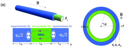
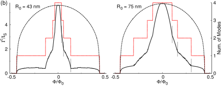
Figure 1: (a) Left: Schematics of a semiconducting NW (green) fully coated by a superconducting shell (blue) and threaded by a longitudinal magnetic field $B$. Right: The cross section defines an effectively insulating region (white) of radius $R_{\text{in}}$, a semiconducting layer of thickness $d_{\text{semi}}=R_{0}-R_{\text{in}}$ and a superconducting shell of thickness $d_{\text{sc}}=R_{\text{out}}-R_{0}$. Within the hollow-core approximation Vaitiekenas et al. (2020) the thickness of the semiconducting layer is assumed to be $d_{\text{semi}}\approx 0$. This fixes the radial coordinate $r=R_{0}$ and the external magnetic flux $\Phi=\pi R_{0}^{2}B$. Bottom: Schematics of an SNS junction where a normal (N) region of length $L_{N}$ is encapsulated between two superconducting (S) regions of length $L_{S}$ and phase difference $\varphi_{0}$. (b) Flux-tunable critical current, $I^{\text{c}}$, (in units of $I_{S}=e\Delta_{0}/\hbar$) and number of nondegenerate subgap modes (dotted lines, right axis) within the zeroth lobe, $n=0$. By increasing the magnetic flux, $\Phi$, the number of subgap modes contributing to $I^{\text{c}}$ decreases at each vertical line, ‘kink’ point, giving rise to a stepwise current profile. Dashdotted curves show $I^{\text{c}}(\Phi)=I^{\text{c}}(0)\Delta(\Phi)/\Delta_{0}$. Similar characteristics can be seen for $n\neq 0$ lobes.

Full-shell nanowires (NWs), where a semiconducting core fully coated by an epitaxial superconductor Krogstrup et al. (2015) is threaded by an external magnetic flux $\Phi$, have recently been explored as a promising novel platform to generate Majorana zero modes Lutchyn et al. (2018); Vaitiekenas et al. (2020); Peñaranda et al. (2020); Valentini et al. (2021, 2022). Their interest, however, goes beyond Majorana physics since the full-shell geometry gives rise to a great deal of new physics, including nontrivial $\Phi$-dependent superconductivity Vaitiekėnas et al. (2020) owing to the Little-Parks (LP) effect Little and Parks (1962); Parks and Little (1964), as well as analogs of subgap states in vortices Kopasov and Mel’nikov (2020); San-Jose et al. (2022).

While JJs based on full-shell NWs start to attract experimental attention Sabonis et al. (2020); Razmadze et al. (2020); Kringhøj et al. (2021); Ibabe et al. (2022), a theoretical understanding is still lacking. The purpose of this Letter is to fill this void by presenting calculations of superconductor-normal-superconductor (SNS) junctions based on hollow-core full-shell NWs [Figs. 1(a)]. Our main result is the demonstration of critical supercurrent, $I^{\text{c}}$, tunability as a function of $\Phi$ [Fig. 1(b)]. Specifically, we find a stepwise decrease with $\Phi$-dependent features which can be analytically understood in terms of the underlying orbital degeneracies and symmetries of the ABS spectrum. The $\Phi$-dependence reported here is completely unrelated to the LP modulation of the superconducting pairing gap, and can be observed even when there is no LP modulation. In stark contrast to previously reported flux-induced supercurrents which are LP-dominated Sabonis et al. (2020); Vekris et al. (2021). Our findings have important implications in recently proposed transmon qubit designs Sabonis et al. (2020), where flux tunability could offer further functionalities.

Nanowire model.– We first consider a cylindrical semiconducting NW, unit vectors $({\hat{e}_{r}},{\hat{e}_{\varphi}},{\hat{e}_{z}})$, in the presence of an axial magnetic field ${\vec{B}}=B{\hat{e}_{z}}$ and with finite SO coupling. Assuming that the electrons are strongly confined near the surface of the NW (hollow-core approximation Vaitiekenas et al. (2020)), we fix the radial cylindrical coordinate $r=R_{0}$ [Fig. 1(a)], thus the flux that threads the NW cross-section is $\Phi=\pi BR_{0}^{2}$ and the vector potential is $\vec{A}=A_{\varphi}{\hat{e}_{\varphi}}=\frac{\Phi}{2\pi R_{0}}{\hat{e}_{\varphi}}$. The Hamiltonian then reads

$$H_{0}(\vec{A})=\frac{(\vec{p}+eA_{\varphi}{\hat{e}_{\varphi}})^{2}}{2m^{*}}-\mu+H_{\text{SO}},$$ (1)

with $\vec{p}=(p_{\varphi},p_{z})=(-\frac{i\hbar}{R_{0}}\partial_{\varphi},-i\hbar\partial_{z})$ being the momentum operator, $m^{*}$ the effective mass and $\mu$ the chemical potential. Assuming radial inversion symmetry breaking, namely $\vec{\alpha}=\alpha{\hat{e}_{r}}$, the Rashba SO Hamiltonian is Bringer and Schäpers (2011) $H_{\text{SO}}=H^{z}_{\text{SO}}+H^{\perp}_{\text{SO}}=\frac{\alpha}{\hbar}\left[p_{z}\sigma_{\varphi}-(p_{\varphi}+eA_{\varphi})\sigma_{z}\right]$, with the spin-1/2 Pauli matrices $\sigma_{\varphi}=\sigma_{y}\cos(\varphi)-\sigma_{x}\sin(\varphi)$, $\sigma_{z}$ and the SO coupling $\alpha$.

Owing to the proximity effect, the semiconducting core acquires superconducting pairing terms. Importantly, they are modulated by $\Phi$ through the LP effect , which induces a winding of the superconducting phase in the shell around the nanowire axis $\bm{\Delta}=\Delta e^{in\varphi}$. Both the amplitude $\Delta$ and the winding (fluxoid) number $n$ depend implicitly on $\Phi$ (Appendix A). Defining the normalized flux $n_{\Phi}=\Phi/\Phi_{0}$, with $\Phi_{0}=h/2e$, the winding number reads $n=\left\lfloor{n_{\Phi}}\right\rceil$. Thus, we measure deviations from integer fluxes through the variable $\phi=n-n_{\Phi}$, with $\phi=0$ corresponding to the middle of a so-called LP lobe Vaitiekėnas et al. (2020). In what follows $\Delta(\Phi=0)\equiv\Delta_{0}$.

In the Nambu basis $\Psi=(\psi_{\uparrow},\psi_{\downarrow},\psi^{\dagger}_{\downarrow},-\psi^{\dagger}_{\uparrow})$, the Bogoliubov-de-Gennes (BdG) Hamiltonian $H_{\rm BdG}$ can be decomposed as a set of decoupled one-dimensional models Sriram et al. (2019); Tserkovnyak and Halperin (2006); Richter et al. (2008); Bringer and Schäpers (2011); Holloway et al. (2015) labelled in terms of the eigenvalues $m_{j}$ of a generalized angular momentum operator Lutchyn et al. (2018) $\hat{J}_{z}(n)=-i\partial_{\varphi}+\frac{1}{2}\sigma_{z}+\frac{1}{2}n\tilde{\tau}_{z}$, with $\tilde{\tau}$ acting in Nambu space. Physically acceptable wavefunctions require that Vaitiekenas et al. (2020) $m_{j}=\pm 1/2$, $\pm 3/2$, $\ldots$ for even $n$ and $m_{j}=0$, $\pm 1$, $\ldots$ for odd $n$. The resulting BdG Hamiltonians  can be conveniently written as:

$$H_{\rm BdG}=\left(\begin{array}[]{cc}H_{A}&H^{z}_{\text{SO}}\\ -H^{z}_{\text{SO}}&H_{B}\\ \end{array}\right),$$ (2)

with $H^{z}_{\text{SO}}=-\alpha\partial_{z}\tilde{\tau}_{z}$, and

$$H_{A}=\left(\begin{array}[]{cc}\frac{p_{z}^{2}}{2m^{*}}+V_{1}&\Delta\\ \Delta&-\frac{p_{z}^{2}}{2m^{*}}+V_{2}\\ \end{array}\right).$$ (3)

The Hamiltonian $H_{B}$ is obtained by substituting $V_{1}\rightarrow V_{3}$, $V_{2}\rightarrow V_{4}$, and the potential terms are ($\hbar=1$)

$$V_{1(2)}(\phi) = V^{0}_{1(2)}+\delta^{+}_{m_{j}}(\phi)\pm\frac{1}{8m^{*}R^{2}_{0}}\phi^{2},$$

$$V_{3(4)}(\phi) = V^{0}_{3(4)}+\delta^{-}_{m_{j}}(\phi)\pm\frac{1}{8m^{*}R^{2}_{0}}\phi^{2}.$$ (4)

At $\phi=0$, the effective potentials are $V^{0}_{1(3)}=-\mu+\frac{(1\mp 2m_{j})^{2}}{8m^{*}R_{0}^{2}}+\frac{(1\mp 2m_{j})\alpha}{2R_{0}}$, with $V^{0}_{2}=-V^{0}_{1}$ and $V^{0}_{4}=-V^{0}_{3}$. Small deviations from integer fluxes ($\phi=0$) are captured by the linear terms

$$\delta^{\pm}_{m_{j}}(\phi)=\frac{-2m_{j}\pm 1}{4m^{*}R^{2}_{0}}\phi\pm\frac{\alpha}{2R_{0}}\phi.$$ (5)

At $\phi=0$, the terms $V^{0}_{1}(m_{j})$ and $V^{0}_{3}(m_{j})$ govern the chemical potential at which the levels belonging to $H_{A}$ and $H_{B}$ respectively cross zero energy. The important quantity is the chemical potential difference which depends on the angular motion and is equal to $V^{0}_{3}(m_{j})-V^{0}_{1}(m_{j})=m_{j}/m^{*}R_{0}^{2}+2m_{j}\alpha/R_{0}$. Interestingly, when $\alpha=0$ the energy levels of $H_{A}(m_{j}+1)$ and $H_{B}(m_{j})$ are degenerate because $V^{0}_{1}(m_{j}+1)=V^{0}_{3}(m_{j})$, therefore, levels belonging to different $m_{j}$ modes cross zero energy simultaneously.

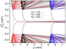
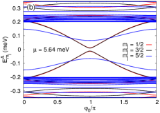
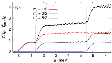
Figure 2: (a) Zero-flux energies of $H_{A}(m_{j})$ as a function of chemical potential at $\varphi_{0}=\pi$ with $E^{A}_{-m_{j}}=-E^{B}_{m_{j}}$ and $E^{B}_{m_{j}}=E^{A}_{m_{j}+1}$. As $\mu$ increases the vertical lines define the effective potential $V^{0}_{1}(m_{j})\approx 0$ for $m_{j}=1/2$, 3/2, 5/2 respectively. The small oscillatory dependence around $E^{A}_{m_{j}}=0$ is generic in SNS junctions governed by the BdG equation. (b) Energies of $H_{A}(m_{j})$ as a function of $\varphi_{0}$. There are in total 5 positive subgap levels dispersing with $\varphi_{0}$: $E^{A}_{1/2}$, $E^{B}_{1/2}=E^{A}_{3/2}$ and $E^{B}_{3/2}=E^{A}_{5/2}$. Any other pair of levels has a non-zero spacing but this can be too small to resolve it. The degeneracies are lifted for $\alpha\neq 0$ (Appendix E). (c) Critical current, $I^{\text{c}}$, and $m_{j}$ contributions $I^{\text{c}}_{(m_{j})}=I^{\text{c}}_{-m_{j}}+I^{\text{c}}_{m_{j}}$. Vertical lines are the same as in (a). Parameters: $L_{S}=2000$ nm, $L_{N}=100$ nm, $R_{0}=43$ nm, $\alpha=0$, $\Delta=\Delta_{0}=0.2$ meV and $I_{S}=e\Delta_{0}/\hbar$.

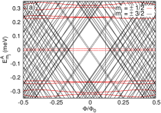
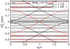
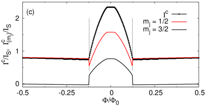
Figure 3: (a) Energies of $H_{A}(m_{j})$ as a function of magnetic flux at $\varphi_{0}=\pi$ with $E^{A}_{-m_{j}}=-E^{B}_{m_{j}}$ and $E^{B}_{m_{j}}=E^{A}_{m_{j}+1}$. Dotted lines show how the anticrossing points at $E^{A}_{m_{j}}\approx 0$, $\Phi=0$ evolve with flux. Vertical lines define the flux, $\Phi/\Phi_{0}=\pm 0.125$, where the contribution of a subgap mode of $H_{B}(m_{j})$ or $H_{A}(m_{j}+1)$ is suppressed. (b) Energies of $H_{A}(m_{j})$ as a function of $\varphi_{0}$ at $\Phi/\Phi_{0}=0.15$. (c) Critical current, $I^{\text{c}}$, and $m_{j}$ contributions $I^{\text{c}}_{(m_{j})}=I^{\text{c}}_{-m_{j}}+I^{\text{c}}_{m_{j}}$. Vertical lines are the same as in (a). Parameters: $L_{S}=2000$ nm, $L_{N}=100$ nm, $R_{0}=43$ nm, $\alpha=0$, $\Delta=\Delta_{0}=0.2$ meV, $\mu=2.5$ meV and $I_{S}=e\Delta_{0}/\hbar$.

SNS junction.– The SNS junction is defined by including a spatial dependence of the pairing potential of the form $\Delta_{R/L}=\Delta e^{i(n\varphi\pm\varphi_{0}/2)}$, where $\varphi_{0}$ is the superconducting phase difference and R/L denotes two right/left superconducting (S) regions of length $L_{S}$. The normal (N) region is defined as $\Delta_{N}=0$ within a length $L_{N}$ Cayao et al. (2018). For simplicity, we assume in the main text that $\mu$ is position-independent (uniform) along the $z$ direction. In a realistic experimental implementation, however, the superconducting full shell is expected to screen any external electric field making gating only effective in the N region. This configuration can be modelled as a smooth spatial variation of the chemical potential in the N region (Appendix B). A uniform chemical potential results in the maximum critical current, whereas the current is reduced as the potential offset between the N and S regions increases.

The supercurrent-phase relationship $I(\varphi_{0})$ can be written in terms of independent contributions for each angular number $m_{j}$. Assuming zero temperature, it reads

$$I(\varphi_{0})=\sum_{m_{j}}I_{m_{j}}(\varphi_{0})=-\frac{e}{\hbar}\sum_{m_{j}}\sum_{k>0}\frac{dE_{k,m_{j}}}{d\varphi_{0}},$$ (6)

where $E_{k,m_{j}}$ are the positive BdG eigenvalues which are computed numerically by discretizing the SNS junction . The critical current is $I^{\text{c}}=\text{max}[I(\varphi_{0})]$ and can be decomposed into different orbital components $I^{\text{c}}_{m_{j}}$.

Zero-flux SNS junction.– We start the analysis of the SNS junction for $\Phi=0$, and plot the energies of $H_{A}(m_{j})$ in Fig. 2(a). BdG levels are induced in a systematic way in the superconducting gap by increasing the chemical potential $\mu$, hence tuning the number of active modes in the junction. The vertical lines in Fig. 2(a) correspond to the effective potential $V^{0}_{1}(m_{j})\approx 0$ specifying the required $\mu$ that shifts an extra mode into the gap. Because of the relatively small normal region considered here, $L_{N}=100$ nm, each of $H_{A}(m_{j})$ and $H_{B}(m_{j})$ can contribute a single subgap mode. The degree of $\varphi_{0}$-dispersion depends on the exact value of $\mu$ and some subgap levels can be quasi-degenerate [Fig. 2(b)].

Figure 2(c) illustrates the critical current together with the $m_{j}$ contributions. The vertical lines have the same meaning as in Fig. 2(a), so when an extra energy level shifts into the gap the critical current exhibits a noticeable increase. Small fluctuations of the current, which are more pronounced at larger $\mu$ values, are due to the small variations of the subgap levels at $E^{A}_{m_{j}}\approx 0$ as shown in Fig. 2(a). The details of the current profile depend on the characteristic length scales ($R_{0}$, $L_{S}$, $L_{N}$) of the SNS junction. A smooth barrier-like local potential $\mu(z)$ on top of the global $\mu$ allows us to precisely control the number of active modes by depleting the N region (Appendix B).

Flux tunable critical current.– We proceed to study finite flux effects for an SNS junction governed by Eq. (2). At small fluxes the linear terms $\delta^{\pm}_{m_{j}}(\phi)$ [Eq. (5)] are the dominant ones, and produce a shift of the corresponding zero-flux energies. The main physics is illustrated in Fig. 3(a), where we plot the energies of $H_{A}(m_{j})$ as a function of $\Phi$ when only $m_{j}=1/2$, $3/2$ are relevant. The key feature here is that by increasing $\Phi$ the $\Phi=0$ subgap levels which anticross ($\varphi_{0}=\pi$, $E^{A}_{m_{j}}\approx 0$) shift in the quasi-continuum. Although, these levels still anticross when $\Phi\neq 0$, the anticrossing point gradually shifts outside the gap. This is demonstrated clearer in Fig. 3(b) where the energies of $H_{A}(m_{j})$ are plotted versus $\varphi_{0}$. The anticrossing lying outside the gap is due to $E^{B}_{1/2}$, $E^{A}_{3/2}$, [$\delta^{-}_{1/2}(\phi)=\delta^{+}_{3/2}(\phi)\neq 0$] whereas the anticrossing lying in the gap is due to $E^{A}_{1/2}$ for which $\delta^{+}_{1/2}(\phi)=0$. The required magnetic flux to suppress the contribution of a subgap mode of $H_{B}(m_{j})$ or $H_{A}(m_{j}+1)$ is of the order of $(2m_{j}+1)|\phi|\approx 4\Delta m^{*}R^{2}_{0}$, therefore, larger $m_{j}$ subgap modes are suppressed at smaller flux values. This simplified approach assumes that $\mu$ is large enough so that the corresponding anticrossing point lies at zero energy. In Fig. 3(c), $\Phi/\Phi_{0}\approx\pm 0.125$ defines a crossover, kink point, which is formed so long as a subgap mode is suppressed, and then the current versus flux drops at a smaller overall rate. For the particular example in Fig. 3(c) $\delta^{+}_{1/2}(\phi)=0$, so this rate is zero but as shown below the physics is more interesting for larger $m_{j}$ values.

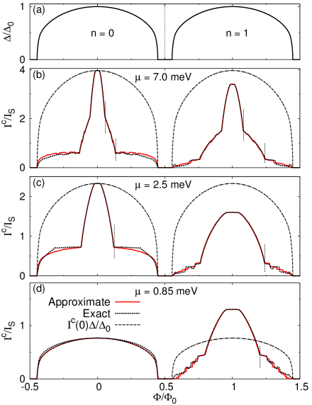
Figure 4: (a) Pairing potential versus flux for lobes $n=0$ and $n=1$. (b), (c), (d) Exact and approximate currents calculated with $\Delta$ as in (a). Vertical lines indicate kink points where the number of non-degenerate subgap modes decreases by one. For $n=0$, $\mu=7$ meV and $\Phi=0$, there are 3 subgap modes coming from $m_{j}=1/2$, $3/2$, $5/2$. For $\Phi\neq 0$ two kink points are formed when $E^{A}_{5/2}$ and $E^{A}_{3/2}$ shift successively outside the gap. For $n=0$, $\mu=2.5$ meV and $\Phi=0$, there are 2 subgap modes coming from $m_{j}=1/2$, $3/2$, thus, for $\Phi\neq 0$ one kink point is formed when $E^{A}_{3/2}$ shifts outside the gap. For $n=0$, $\mu=0.85$ meV the single mode current ($m_{j}=1/2$) is LP-dominated because $\delta^{+}_{1/2}=0$. For the same reason the mode $E^{A}_{1/2}$ remains to a good approximation in the gap independent of $\Phi$ for any $\mu$. Approximate results for $n=0$, $\mu=15$ meV and $m_{j}=1/2$, $3/2$, $5/2$, $7/2$ are shown in Fig. 1(b). Similar arguments are valid for $n=1$ but now the current is never LP-dominated. At $\Phi=\Phi_{0}$ and $\mu=7$ meV the angular numbers $m_{j}=0$, 2 are relevant while for $\mu=2.5$, 0.85 meV only $m_{j}=0$ is relevant. Because $\delta^{+}_{m_{j}}\neq 0$ all modes shift outside the gap leading to a more ‘noisy’ current profile compared to $n=0$. A weak SO coupling, $\alpha\neq 0$, does not alter the basic characteristics (Appendix C). Parameters: $L_{S}=2000$ nm, $L_{N}=100$ nm, $R_{0}=43$ nm, $\alpha=0$, $\Delta_{0}=0.2$ meV, $\xi=80$ nm, $d_{\text{sc}}=0$ and $I_{S}=e\Delta_{0}/\hbar$.

We now include the LP modulation of the pairing amplitude (Appendix A) $\Delta=\Delta(n,\Phi,R_{0},d_{\text{sc}},\xi)$, where $\xi$ is the coherence length of the superconducting shell. When the shell thickness $d_{\text{sc}}\rightarrow 0$, then $\Delta$ depends on $\phi$ instead of $\Phi/\Phi_{0}$. We consider a destructive regime in which $\Delta=0$ near the boundaries of the lobes and $\Delta=\Delta_{0}$ at the center of the lobes [Fig. 4(a)].

The flux tunable critical current is presented in Fig. 4. The current at $\phi=0$ (namely $n_{\Phi}=\Phi/\Phi_{0}=0$, 1) depends on $\mu$ which specifies the number and position of subgap modes in the superconducting gap. Once this number is fixed, by varying $\Phi$ with respect to the centre of the lobe the current is gradually reduced, and a kink point is formed at the flux where the contribution of a subgap mode vanishes. The current for $n=1$ exhibits similar characteristics to that for $n=0$ but with noticeable differences, e.g., the $\phi=0$ currents in the two lobes are different even when $\Delta$ is the same. The reason is the different potentials $V_{1(2)}$ involved in the BdG Hamiltonian. According to Fig. 4, the flux dependence of $\Delta$ cannot be used to explain $I^{\text{c}}(\Phi)$. The formula Sabonis et al. (2020); Vekris et al. (2021) $I^{\text{c}}(\Phi)\approx I^{\text{c}}(\Phi=0)\Delta(\Phi)/\Delta_{0}$ completely fails to capture the correct flux dependence of $I^{\text{c}}$ in the multi-mode regime . Instead, a good approximation to the current is obtained by assuming the approximate flux dependence of the BdG levels, $E_{m_{j}}(\phi)\approx E_{m_{j}}(\phi=0)\Delta(\phi)/\Delta_{0}+\delta^{\pm}_{m_{j}}(\phi)$, with $E_{m_{j}}(\phi=0)$ being the exact $\phi=0$ BdG levels, and using Eq. (6) with all positive levels included. When the terms $\delta^{\pm}_{m_{j}}(\phi)$ become smaller, e.g., by increasing $R_{0}$, the kink points shift at higher flux values [Fig. 1(b)].

Simplified SNS junction model.– The approximate results presented in Fig. 4 reveal the vital role of the linear terms $\delta^{\pm}_{m_{j}}(\phi)$. To obtain further qualitatively insight we develop a simplified model where $I(\varphi_{0})$ is governed by the ABSs:

$$E_{\pm,k}(\varphi_{0},\Phi)=\pm\Delta(\Phi)\sqrt{1-\tau_{k}\sin^{2}(\varphi_{0}/2)}+w_{k}\Phi/\Phi_{0},$$ (7)

$k=1$, 2, $\ldots$ $M$ is the number of ABSs and the parameters $0<\tau_{k}\leq 1$ model the transparency of the SNS junction. The linear terms $w_{k}\Phi/\Phi_{0}$ with $w_{k}=(k-1)/2m^{*}R^{2}_{0}$ play the same role as $\delta^{+}_{m_{j}}(\phi)$ [Eq. (5)] for $\alpha=0$ (Appendix C). The exact $\varphi_{0}$-dispersion is not important and we adopt Eq. (7) for simplicity and to illustrate the crossover from the LP-regime to the stepwise regime.

For $\tau_{k}=1$ and when all $w_{k}$ are zero, the analytically computed supercurrent [Eq. (6)] can be written as $MI_{Z}(\varphi_{0})$, and for the critical current in a spinfull junction we recover the standard result Beenakker and van Houten (1991); Furusaki et al. (1992) $I^{\text{c}}(\Phi)=Me\Delta(\Phi)/\hbar=I^{\text{c}}(0)\Delta(\Phi)/\Delta_{0}$; the flux dependence of $I^{\text{c}}$ is due solely to the LP modulation of $\Delta$. A completely different situation occurs when $w_{k}\neq 0$. Now within the flux range $0\leq w_{k}\Phi/\Phi_{0}\leq\Delta$ we define the corresponding flux dependent phase $\theta_{k}=\theta_{k}(\Phi)$ satisfying $E_{-,k}(\theta_{k})=0$ with $0\leq\theta_{k}\leq\pi$. As $\Phi$ increases and the levels $E_{-,k}(\theta_{k})$ shift gradually upwards a decrease in $I^{\text{c}}(\Phi)$ is expected. A simple inspection shows that $I^{\text{c}}(\Phi)$ is equal to the larger of $kI_{Z}(\theta_{k})$ and $(k-1)I_{Z}(\theta_{k-1})$, with $k\rightarrow k-1$ as the flux increases. For the flux

$$\frac{\Phi}{\Phi_{0}}=\Delta(\Phi)\sqrt{\frac{k^{2}-(k-1)^{2}}{k^{2}w^{2}_{k}-(k-1)^{2}w^{2}_{k-1}}},$$ (8)

the currents satisfy

$$kI_{Z}(\theta_{k})=(k-1)I_{Z}(\theta_{k-1}),$$ (9)

then a kink point is formed and the number of ABSs contributing to the critical current decreases by one . Because $\theta_{k-1}$ varies with flux slower than $\theta_{k}$, Eq. (9) leads to a stepwise decrease of the current. For very large $R_{0}$ ($>150$ nm), $w_{k}$ are vanishingly small and the current steps/kink points are formed at flux values lying (very) near the boundaries of the lobe; in this case $I^{\text{c}}(\Phi)$ is trivially LP-dominated. In contrast, experimentally reported Valentini et al. (2021, 2022); Vekris et al. (2021); Ibabe et al. (2022) $R_{0}$ ($\lesssim 100$ nm) guarantee a stepwise decrease. In Appendix C we generalize the simplified model to $\tau_{k}<1$ and make a connection with the exact BdG model in Appendix D.

Conclusion.– The critical supercurrent in full-shell nanowire Josephson junctions exhibits a stepwise dependence as a function of an external magnetic flux. This flux dependence has striking features, unrelated to the Little-Parks modulation of the superconducting pairing. The position of the steps depends on the underlying symmetries of the transverse channels contributing to the supercurrent and it is thus gate-tunable. This prediction should be robust for low-disordered samples and specially in the low-flux range, $n=0$ with $\Phi\lesssim\Phi_{0}/2$, where transverse channel interference due to $m_{j}$ mixing, not included here, should be negligible. Such effects, similar to Fraunhofer-like interference in diffusive many-channel planar junctions Cuevas and Bergeret (2007) and few-channel hybrid NW junctions Gharavi et al. (2014); Zuo et al. (2017); Sriram et al. (2019), could be of relevance in the first LP lobe, $n=1$ at $\Phi\approx\Phi_{0}$, and lead to further structures in $I^{\text{c}}$. Experiments able to discriminate between the flux modulation of the gap and the intrinsic subgap structure, for example, Joule heating experiments Ibabe et al. (2022), could be an interesting platform to explore the effects predicted here. Our findings could be also of relevance for transmon qubits based on full shell NWs Sabonis et al. (2020), where flux tunability of the Josephson coupling under an axial magnetic field (without requiring split-junction geometries) could lead to novel functionalities.

Appendix A Superconducting pairing potential

The superconducting pairing potential, $\Delta$, due to the Little-Parks effect Little and Parks (1962); Parks and Little (1964) acquires a flux dependence. If $\Delta_{0}$ is the value of $\Delta$ at $\Phi=0$ then according to Abrikosov-Gor’kov Abrikosov (1969); Skalski et al. (1964) a pair-breaking term $\Lambda$ results in the following modulation of $\Delta$:

$$\ln\frac{\Delta}{\Delta_{0}} = -\frac{\pi}{4}\frac{\Lambda}{\Delta},\quad\Lambda\leq\Delta,$$

$$\ln\frac{\Delta}{\Delta_{0}} = -\ln\left(\frac{\Lambda}{\Delta}+\sqrt{(\Lambda/\Delta)^{2}-1}\right)+\frac{\sqrt{(\Lambda/\Delta)^{2}-1}}{2(\Lambda/\Delta)}-\frac{\Lambda}{2\Delta}\arctan\frac{1}{\sqrt{(\Lambda/\Delta)^{2}-1}},\quad\Lambda\geq\Delta.$$ (10)

Within a Ginzburg-Landau theory Sternfeld et al. (2011); Shah and Lopatin (2007); Dao and Chibotaru (2009); Schwiete and Oreg (2010) the magnetic flux dependence of $\Lambda$ can be determined from the approximate expression

$$\Lambda(\Phi)\approx\frac{\xi^{2}k_{B}T_{c}}{\pi R^{2}_{0}}\left[4\left(n-\frac{\Phi}{\Phi_{0}}\right)^{2}+\frac{d^{2}_{\text{sc}}}{R^{2}_{0}}\left(\frac{\Phi^{2}}{\Phi^{2}_{0}}+\frac{n^{2}}{3}\right)\right].$$ (11)

The parameter $\xi$ denotes the coherence length of the superconducting shell which has thickness $d_{\text{sc}}$, $n$ is the lobe index, $T_{c}$ is the critical temperature at zero flux, and $k_{B}T_{c}=\Delta_{0}/1.76$ Skalski et al. (1964) where $k_{B}$ is Boltzmann’s constant. In our work, we focus on $R_{0}\gg d_{\text{sc}}$ and for simplicity we set $d_{\text{sc}}=0$; a small non-zero $d_{\text{sc}}$ introduces only minor corrections to the final magnetic flux dependence of $\Delta$. The numerical solution to Eq. (A) is well-known and can be found in the literature, for example, in Ref. Skalski et al., 1964. In the limit $\Lambda\rightarrow\Delta_{0}/2$ the pairing potential nearly vanishes, $\Delta\rightarrow 0$, we then set $\Delta=0$ for $\Lambda\geq\Delta_{0}/2$ to model a destructive regime. One example of the pairing potential for $R=43$ nm, $\xi=80$ nm, $d_{\text{sc}}=0$ is shown in Fig. 4(a) of the main article.

Appendix B SNS junction with spatially dependent chemical potential

In the main article the chemical potential, $\mu$, is taken to be constant (spatially independent) along the SNS junction. This configuration simplifies the theoretical analysis but it might be difficult to realize experimentally. For this reason, we consider one more configuration where the chemical potential is spatially dependent, i.e., $\mu=\mu(z)$. In this context, we assume that an electrostatic gate voltage tunes the chemical potential in the normal (N) region with respect to the potential in the superconducting (S) regions, thus, creating a potential offset between the N and S regions. The spatial profile of the chemical potential along the SNS junction is written as

$$\mu(z)=\mu_{0}-\mu_{\text{pot}}f(z),$$ (12)

where the function $f(z)$ is expected to depend on the exact geometry of the junction, the microscopic details of the S-N interfaces, and the charge distribution in the junction. We consider a continuous variation across the S-N interfaces and assume that

$$f(z)=\frac{1}{K\left(\frac{(z-z_{0})^{2}}{2D^{2}}\right)},$$ (13)

where for the function $K$ we take either $K=\exp$ or $K=\cosh$, $z_{0}=0$ is the centre of the N region, and $\mu_{\text{pot}}$ ($\geq 0$) determines the potential offset. This offset is maximum in the centre of the N region and the parameter $D$ controls the length scale in which the chemical potential varies along the SNS junction. As shown below, for a large $\mu_{\text{pot}}$ ($\approx\mu_{0}$) the critical current vanishes whereas it is maximum when $\mu_{\text{pot}}\approx 0$. The results in the main article are for $\mu_{\text{pot}}=0$.

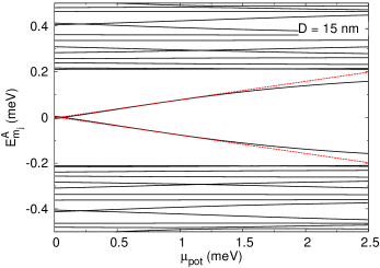
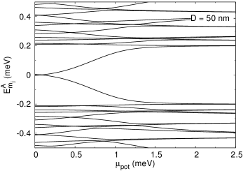
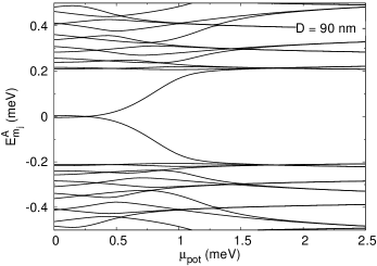
Figure 5: Zero-flux energies of $H_{A}$ [Eq. (3) main article] as a function of $\mu_{\text{pot}}$ at phase difference $\varphi_{0}=\pi$ for $m_{j}=1/2$ and $K=\cosh$, with $E^{A}_{-m_{j}}=-E^{B}_{m_{j}}$ and $E^{B}_{m_{j}}=E^{A}_{m_{j}+1}$. Dashed curves for $D=15$ nm are approximate energies derived from a two-level model described in the text. Parameters: $\mu_{0}=0.9$ meV, $L_{S}=2000$ nm, $L_{N}=100$ nm, $R_{0}=43$ nm, $\alpha=0$, $\Delta=\Delta_{0}=0.2$ meV.

The effect of a nonzero $\mu_{\text{pot}}$ on the energy spectra can be more easily understood in the regime of small $\mu_{0}$, so that to a good approximation only the Hamiltonian $H_{A}$ [Eq. (3) main article] is relevant with $m_{j}=1/2$. One case illustrated in Fig. 5 demonstrates that increasing $\mu_{\text{pot}}$ shifts the subgap levels near the edge of the superconducting gap. This shift in turn reduces the overall degree of $\varphi_{0}$-dispersion and consequently the critical current. Provided $D$ and $\mu_{\text{pot}}$ are small the term $-\mu_{\text{pot}}f(z)$ can be treated within a perturbative two-level model, $H_{A}+\sigma_{z}\mu_{\text{pot}}f(z)$, using for basis states the (two) subgap states at $\mu_{\text{pot}}=0$. Some results of this approximate model are presented in Fig. 5 for $D=15$ nm; the agreement with the exact result is particularly good for small values of $\mu_{\text{pot}}$ and the correct linear behaviour is predicted. The two-level model can also predict the correct $\varphi_{0}$-dispersion, however, by increasing $D$ the model becomes quickly inaccurate. For example, when $D=50$ nm and $\mu_{\text{pot}}\approx 1$ meV about 60 basis states are needed to achieve the same convergence as for $D=15$ nm.

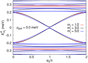
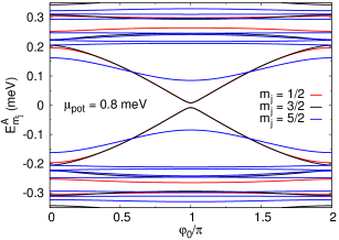
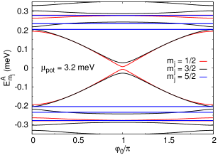
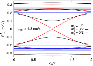
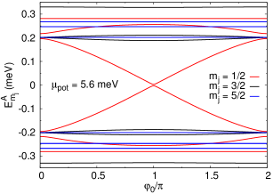
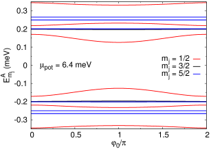
Figure 6: Zero-flux energies of $H_{A}$ [Eq. (3) main article] as a function of phase difference $\varphi_{0}$ for $K=\cosh$, with $E^{A}_{-m_{j}}=-E^{B}_{m_{j}}$ and $E^{B}_{m_{j}}=E^{A}_{m_{j}+1}$. Parameters: $D=70$ nm, $\mu_{0}=6.5$ meV, $L_{S}=2000$ nm, $L_{N}=100$ nm, $R_{0}=43$ nm, $\alpha=0$, $\Delta=\Delta_{0}=0.2$ meV.

A more general configuration is now examined when the energy levels lying in the superconducting gap correspond to different $m_{j}$ numbers. Some typical energy spectra of $H_{A}$ are plotted in Fig. 6. At $\mu_{\text{pot}}=0$ the subgap levels correspond to $m_{j}=1/2$, $3/2$ and $5/2$, thus, there are 5 positive levels: $E^{A}_{1/2}$, $E^{B}_{1/2}$, $E^{A}_{3/2}$, $E^{B}_{3/2}$ and $E^{A}_{5/2}$ with the degeneracies $E^{B}_{1/2}=E^{A}_{3/2}$ as well as $E^{B}_{3/2}=E^{A}_{5/2}$. As shown in Fig. 6, increasing $\mu_{\text{pot}}$ tends to shift the subgap levels outside (near the edge of) the gap in a systematic way, so levels which correspond to larger $m_{j}$ shift outside the gap at smaller values of $\mu_{\text{pot}}$. Consequently, the number of active subgap levels in the SNS junction can be controlled at will.

When the levels shift outside the gap the critical current decreases and eventually complete suppression occurs when $\mu_{\text{pot}}\approx\mu_{0}$ (Fig. 7). The exact form of $f(z)$ determines the details of the process. Specifically, the decrease of the current is not necessarily monotonic and steps can be formed because the different $m_{j}$ levels are not affected equally by the potential term $\mu_{\text{pot}}$.

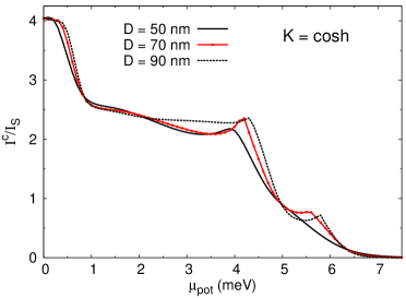
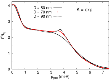
Figure 7: Zero-flux critical current as a function of $\mu_{\text{pot}}$. Parameters: $\mu_{0}=6.5$ meV, $L_{S}=2000$ nm, $L_{N}=100$ nm, $R_{0}=43$ nm, $\alpha=0$, $\Delta=\Delta_{0}=0.2$ meV, $I_{S}=e\Delta_{0}/\hbar$.

Appendix C Simplified SNS junction model

In this section we present in some detail the simplified model introduced in the main article. The subgap modes are written as follows ($\hbar=1$)

$$E_{\pm,k}(\varphi_{0},\Phi)=\pm\Delta\sqrt{1-\tau_{k}\sin^{2}(\varphi_{0}/2)}+w_{k}\Phi/\Phi_{0},$$ (14)

with $k=1,2\ldots M$,

$$w_{k}=\frac{(k-1)}{2m^{*}R^{2}_{0}},$$ (15)

and $\Delta=\Delta(\Phi)$ everywhere. To avoid confusion we note a few remarks. First, we focus on $w_{k}\geq 0$ and multiply the currents by 2 to account for $\pm m_{j}$. Second, the term $w_{k}\Phi/\Phi_{0}$ results in the same flux dependence as $\delta^{+}_{m_{j}}$ in the main article [Eq. (5)] for the zeroth lobe, $n=0$, and zero SO coupling, $\alpha=0$. The first lobe, $n=1$, can be treated similarly. Finally, the degeneracy $H_{B}(m_{j})=H_{A}(m_{j}+1)$ is not considered in Eq. (14) since this does not change qualitatively the final conclusions.

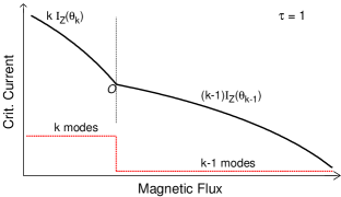
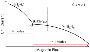
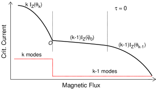
Figure 8: Illustration of flux tunable critical current and number of subgap modes predicted from simplified model, Eq. (14). A single kink point (O) is indicated in each frame. A detailed explanation is given in the text.

When all $w_{k}$ are zero and $\tau_{k}=\tau$ the supercurrent is written as $MI_{Z}(\varphi_{0})$ with

$$I_{Z}(\varphi_{0})=-\frac{e}{\hbar}\frac{\Delta}{2}\frac{\tau\sin\varphi_{0}}{\sqrt{1-\tau\sin^{2}(\varphi_{0}/2)}},$$ (16)

while the phase $\tilde{\varphi}_{0}$ ($\leq\pi$) giving the critical current, $I^{\text{c}}$, can be readily extracted. An interesting remark is that when $w_{k}\neq 0$ the critical current can be expressed with the help of the supercurrent $I_{Z}$. Specifically, for $k\neq 1$ we define within the flux range $\Delta\sqrt{1-\tau}<w_{k}\Phi/\Phi_{0}\leq\Delta$ the corresponding flux-dependent phase $\theta_{k}=\theta_{k}(\Phi)$ satisfying $E_{-,k}(\theta_{k})=0$,

$$\theta_{k}=2\sin^{-1}\sqrt{\frac{1}{\tau}\left(1-\frac{w_{k}^{2}\Phi^{2}}{\Delta^{2}\Phi_{0}^{2}}\right)},$$ (17)

with $0\leq\theta_{k}\leq\pi$. As $\Phi$ increases, $I^{\text{c}}$ follows the $\Delta(\Phi)$ dependence until $\theta_{M}=\tilde{\varphi}_{0}$, but when $\theta_{M}<\tilde{\varphi}_{0}$ the decrease of $I^{\text{c}}$ due to $w_{k}$ needs to be accounted for. Now $I^{\text{c}}$ is equal to the largest of the three terms $kI_{Z}(\theta_{k})$, $(k-1)I_{Z}(\tilde{\varphi}_{0})$ and $(k-1)I_{Z}(\theta_{k-1})$; and as $\Phi$ increases $k\rightarrow k-1$, hence, the number of subgap modes contributing to the current decreases successively by one. This process gives rise to a stepwise current profile and is illustrated in Fig. 8. For $\tau\rightarrow 1$ ($\tilde{\varphi}_{0}\rightarrow\pi$) the flux range where $(k-1)I_{Z}(\tilde{\varphi}_{0})$ needs to be considered vanishes/shrinks, and only the two terms $kI_{Z}(\theta_{k})$, $(k-1)I_{Z}(\theta_{k-1})$ are important. When $kI_{Z}(\theta_{k})=(k-1)I_{Z}(\theta_{k-1})$ a kink point is formed, and using Eq. (17) with

$$I_{Z}(\varphi_{0})=-\frac{e}{\hbar}\Delta\sin(\varphi_{0}/2),$$ (18)

we can determine the corresponding flux value

$$\frac{\Phi}{\Phi_{0}}=\Delta(\Phi)\sqrt{\frac{k^{2}-(k-1)^{2}}{k^{2}w^{2}_{k}-(k-1)^{2}w^{2}_{k-1}}}.$$ (19)

In the opposite limit, $\tau\rightarrow 0$ ($\tilde{\varphi}_{0}\rightarrow\pi/2$), the flux range where $(k-1)I_{Z}(\tilde{\varphi}_{0})$ dominates is maximum and current steps are clearly formed. A kink point is now formed when $kI_{Z}(\theta_{k})=(k-1)I_{Z}(\tilde{\varphi}_{0})$ and the steps become flatter as the flux dependence of $(k-1)I_{Z}(\tilde{\varphi}_{0})$, due to $\Delta(\Phi)$, weakens. In this analysis, because of the special value $w_{1}=0$ we have $I_{Z}(\theta_{1})\rightarrow I_{Z}(\tilde{\varphi_{0}})$ for any value of $\tau$. The $k=1$ mode does not shift with flux and the number of modes drops to zero at the boundaries of the lobe because $\Delta(\Phi)=0$.

In Fig. 9 we plot the critical current for different number of subgap modes $M$. By increasing $M$, extra steps/kink points are formed. Most importantly, the overall current profile is qualitatively the same as that derived from the exact BdG Hamiltonian; see for example Fig. 4 in the main article. For $M=1$, $w_{1}=0$ and the current can be described by the formula $I^{\text{c}}(\Phi)=I^{\text{c}}(0)\Delta(\Phi)/\Delta_{0}$, in stark contrast for $M>1$ this formula is inapplicable. In Fig. 10 we take $M=4$ and plot typical examples of the critical current for three different radii $R_{0}$. For a better comparison, we adjust the coherence length of the shell $\xi$ so that for each $R_{0}$ the pairing potential vanishes when $|\Phi/\Phi_{0}|\gtrsim 0.45$. For illustrative reasons, we also present one case for an unrealistically large radius, $R_{0}=160$ nm. The purpose is to demonstrate how the size of $w_{k}$ affects the overall profile of the current. The role of the terms $w_{k}$ weakens for larger values of $R_{0}$. In particular, when the ratio $1/m^{*}R^{2}_{0}$ becomes vanishingly small the required flux to induce a kink point lies nearly at the boundaries of the lobe. In the regime, $w_{k}\approx 0$, the flux dependence of the current can be accurately described by the formula $I^{\text{c}}(\Phi)=I^{\text{c}}(0)\Delta(\Phi)/\Delta_{0}$; when $\tau=1$ this equals $Me\Delta(\Phi)/\hbar$. Another important observation is that for smaller values of $w_{k}$ the flux dependence of $\theta_{k}$ is weaker. This explains why for a given radius the current steps formed at larger fluxes are in general broader [Fig. 10].

So far in our analysis we have focused on $\tau_{k}=\tau$, but our results can be easily generalized to the most general case when the transparency, $\tau_{k}$, of each individual mode is different. Some analytical expressions for the critical current can again be derived, however, these are not particularly enlightening. The important conclusion is that all the basic features presented in Figs. 9 and 10 are still observable in the most general case. Our analysis is also applicable when the $\varphi_{0}$-dispersion of the subgap modes is different from that specified by Eq. (14). Numerically calculated subgap modes derived from the exact BdG Hamiltonian can equally well demonstrate the physics.

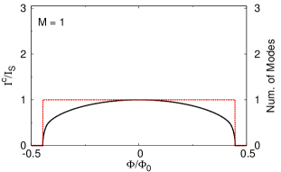
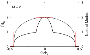
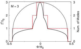
Figure 9: Critical current and number of subgap modes (dotted lines, right axis) derived from simplified model, Eq. (14), with $\tau_{k}=\tau=1$, $R_{0}=43$ nm, $I_{S}=e\Delta_{0}/\hbar$. Dashdotted curves show $I^{\text{c}}(0)\Delta/\Delta_{0}$; this coincides with the critical current for $M=1$. $\Delta$ is calculated from Eq. (A) with $\xi=80$ nm, $d_{\text{sc}}=0$, $\Delta_{0}=0.2$ meV.

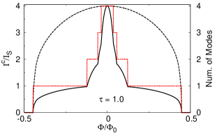
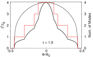
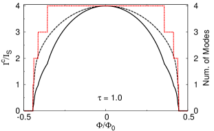
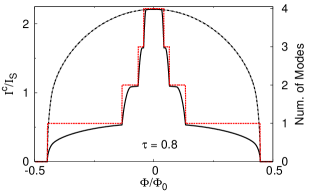
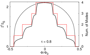
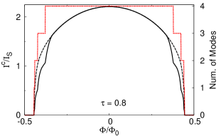
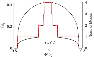
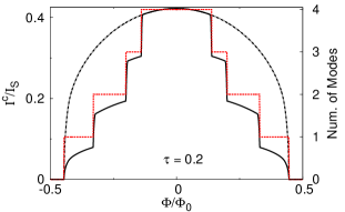
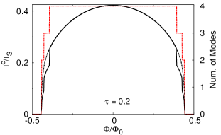
Figure 10: Critical current and number of subgap modes (dotted lines, right axis) derived from simplified model, Eq. (14), with $M=4$, $\tau_{k}=\tau$, $I_{S}=e\Delta_{0}/\hbar$. Dashdotted curves show $I^{\text{c}}(0)\Delta/\Delta_{0}$. First column: $R_{0}=43$ nm, $\xi=80$ nm. Second column: $R_{0}=75$ nm, $\xi=140$ nm. Third column: $R_{0}=160$ nm, $\xi=299$ nm. $\Delta$ is calculated from Eq. (A) with $d_{\text{sc}}=0$, $\Delta_{0}=0.2$ meV.

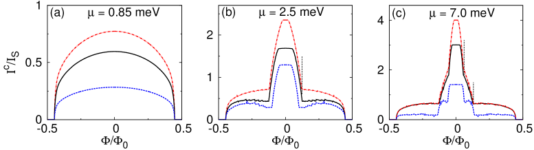
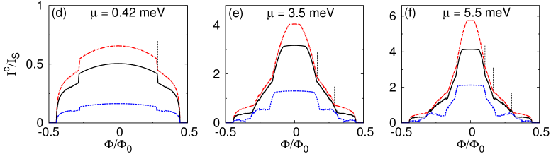
Figure 11: Critical current as a function of magnetic flux calculated with $\Delta$ given by Eq. (A). From upper to lower curve: $\tau_{0}=1$, 0.6, 0.2. Parameters: $L_{S}=2000$ nm, $L_{N}=100$ nm, $\alpha=0$, $\Delta_{0}=0.2$ meV, $d_{\text{sc}}=0$, $I_{S}=e\Delta_{0}/\hbar$. (a)-(c) $R_{0}=43$ nm, $\xi=80$ nm. (d)-(f) $R_{0}=75$ nm, $\xi=140$ nm. Vertical lines indicate kink points for $\tau_{0}=1$. As $\Phi$ increases the number of nondegenerate subgap modes decreases by one at each kink point. The latter, in general, shift for different $\tau_{0}$. At $\Phi=0$ the subgap modes contributing to the current are derived from: (a) $m_{j}=1/2$ (b) $m_{j}=1/2$, 3/2 (c) $m_{j}=1/2$, 3/2, 5/2 (d) $m_{j}=1/2$, 3/2 (e) $m_{j}=1/2$, 3/2, 5/2 (f) $m_{j}=1/2$, 3/2, 5/2, 7/2.

Appendix D Flux tunable current in a reduced transparency junction

In the main article we consider an ideal SNS junction, namely, a transparent junction where there is no explicit physical mechanism to suppress tunnelling between the S and N regions. As introduced above, a spatially dependent chemical potential controls the number of subgap levels as well as the current, but this control is sensitive to the value of $m_{j}$. In this respect, it is interesting to explore how the degree of transparency affects the current when the number of subgap levels remains approximately constant. This can be done using again Eq. (12), but now the parameter $D$ needs to be carefully optimized. This makes the computational procedure inefficient and time consuming. For this reason, we model the transparency of the junction phenomenologically by employing a similar methodology to that presented originally in Ref. Cayao et al., 2017. Specifically, in the BdG Hamiltonian we introduce a dimensionless parameter $\tau_{0}$, with $0<\tau_{0}\leq 1$, which scales the kinetic terms along the z direction ($\tau_{0}p^{2}_{z}/2m^{*}$). We assume this scaling to take place within the N region and an adjacent small part ($x_{S}\approx$ 20 nm $\ll L_{S}$) in the S regions. The transparent limit (main article) corresponds to $\tau_{0}=1$, whereas the opposite limit, $\tau_{0}\approx 0$, is not of interest here since the critical current is almost completely suppressed. Thus, in this work we choose the lower limit to be $\tau_{0}=0.2$ which allows us to capture all the essential characteristics.

For the computations, the kinetic term along z is written as ($\hbar=1$)

$$T_{\text{kin}}=-\frac{1}{2m^{*}}\frac{d}{dz}\left(\tau_{0}(z)\frac{dy(z)}{dz}\right),$$ (20)

where $y(z)$ represents any of the four components of the BdG Hamiltonian. Using centered differences and defining $\tau_{0}$ on the mid lattice points the kinetic term is discretized as follows

$$T_{\text{kin}}\approx b^{i-1}y^{i-1}-[b^{i-1}+b^{i}]y^{i}+b^{i}y^{i+1},$$ (21)

with

$$b^{i}=-\frac{1}{2m^{*}\delta^{2}}\tau_{0}^{i+1/2},\quad b^{i-1}=-\frac{1}{2m^{*}\delta^{2}}\tau_{0}^{i-1/2},$$ (22)

and $\delta$ is the spacing between the lattice points. Here, $b^{i}$ describes hopping between the lattice points $i$ and $i+1$ while $\tau_{0}^{i+1/2}$ is the value of the transparency between these two lattice points. When $\tau_{0}$ is constant the usual finite-difference approximation to the kinetic term is recovered.

We calculate the critical current using the approximation described in the main article and show some representative numerical results in Fig. 11. Note, that as happens with the current suppression versus $\mu_{\text{pot}}$ in Fig. 7, the current suppression versus $\tau_{0}$ at a fixed chemical potential and flux is not always monotonic. As $\tau_{0}$ decreases the basic flux tunable features are well-formed at least for intermediate ($\tau_{0}\approx 0.5$) and somewhat smaller values of $\tau_{0}$. Our calculations within the exact BdG Hamiltonian confirm that this behaviour is robust for different sets of parameters: $R_{0}$, $\mu$ and $x_{S}$. They also indicate that the form of the current steps does not necessarily improve upon decreasing $\tau_{0}$. Although, some steps become more pronounced this cannot be guaranteed to be the general rule. In our SNS junction with energy levels above the gap contributing to the current as well as with an explicit $\mu$ (and/or $\mu_{\text{pot}}$) dependence, the underlying physics is expected to deviate to some degree from the simplified model. Energy levels which lie above the gap at $\Phi=0$ tend to make the steps more ‘noisy’ at $\Phi\neq 0$, and the overall noise is sensitive to the exact values of $\mu$ and $\tau_{0}$. These effects are not captured by the simplified model. The quality of the steps is expected to improve in SNS junctions with shorter N region. Another important aspect, which might be relevant to experimental studies, is that steps formed at larger fluxes can be almost completely suppressed for a relatively large $\tau_{0}$. This effect can lead to the wrong conclusion that the current suppression is due to the LP effect. A rigorous method to disentangle the LP suppression from that caused by $\tau_{0}$ deserves further investigation.

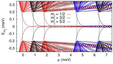
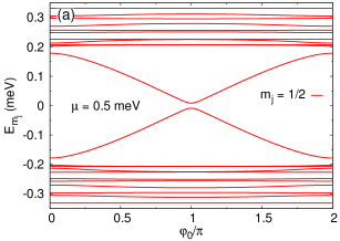
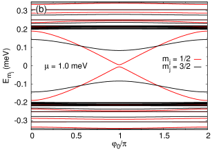
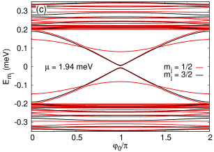
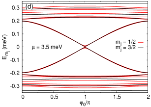
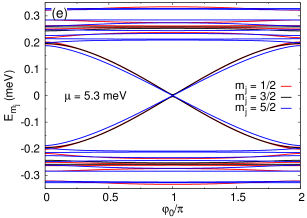
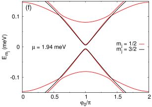
Figure 12: Top frame: Zero-flux energy spectrum of SNS junction as a function of chemical potential at phase difference $\varphi_{0}=\pi$. Energies are derived from $H_{\text{BdG}}$ [Eq. (2) main article] and satisfy $E_{-m_{j}}=-E_{mj}$. Vertical lines define the effective potentials $V^{0}_{1}(m_{j})\approx 0$ and $V^{0}_{3}(m_{j})\approx 0$ for $m_{j}=1/2$, 3/2, 5/2. (a)-(e) Energies as a function of phase difference at different chemical potentials. Only energies lying within the chosen energy range are plotted. (f) Zoom in of (c) showing anticrossing point for $m_{j}=1/2$ due to the SO coupling. Parameters: $L_{S}=2000$ nm, $L_{N}=100$ nm, $R_{0}=43$ nm, $\alpha=20$ meV nm, $\Delta=\Delta_{0}=0.2$ meV.

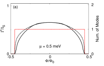
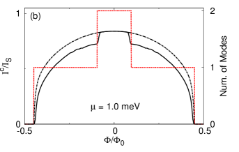
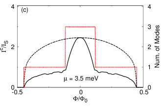
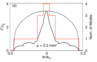
Figure 13: Solid curves show exact critical current, $I^{\text{c}}(\Phi)$, calculated with $\Delta$ given by Eq. (A). Dashdotted curves show $I^{\text{c}}(0)\Delta/\Delta_{0}$. Dotted lines show the number of subgap modes (right axis). Parameters: $L_{S}=2000$ nm, $L_{N}=100$ nm, $R_{0}=43$ nm, $\alpha=20$ meV nm, $\Delta_{0}=0.2$ meV, $\xi=80$ nm, $d_{\text{sc}}=0$, $I_{S}=e\Delta_{0}/\hbar$. At $\Phi=0$ the subgap modes contributing to the current are derived from: (a) $m_{j}=1/2$ (b) $m_{j}=1/2$, 3/2 (c) $m_{j}=1/2$, 3/2 (d) $m_{j}=1/2$, 3/2, 5/2.

Appendix E SNS junction with spin-orbit coupling

In this section we examine the effect of the Rashba spin-orbit (SO) coupling on the flux dependence of the critical current. Our aim is to demonstrate that the current profile presented in Fig. 4 of the main article can still be observed in the presence of weak SO coupling. Analyzing in detail SO effects is beyond the scope of this work.

We consider the chemical potential, $\mu$, to be constant along the SNS junction, thus, as explained above we focus on the resonant case where the critical current is maximum. A nonuniform $\mu$ simply results in a reduced current. A nonzero SO coupling, $\alpha$, shifts further apart the values of $\mu$ at which the energy levels of $H_{A}(m_{j})$ and $H_{B}(m_{j})$ respectively enter the superconducting gap. This shift is of the order of $2m_{j}\alpha/R_{0}$ as can be understood directly from Eqs. (4) in the main article. In addition, when $\alpha\neq 0$ the energies of $H_{A}(m_{j}+1)$ and $H_{B}(m_{j})$ are no longer degenerate, since $V^{0}_{1}(m_{j}+1)\neq V^{0}_{3}(m_{j})$, and when the parameters are tuned so that $(\hbar=1)$

$$\alpha\approx\frac{2m_{j}-1}{4m^{*}R_{0}},$$ (23)

the condition $V^{0}_{1}(m_{j})\approx-\mu$ can be satisfied for $m_{j}>1/2$ (assuming $\Phi=0$). In this regime and at low chemical potentials the critical current is no longer dominated by $m_{j}=1/2$ only, therefore, an enhanced critical current can be observed compared to that for $\alpha=0$. A subtle point is that this enhancement is not due to the actual coupling between $H_{A}(m_{j})$ and $H_{B}(m_{j})$ caused by $H^{z}_{\text{SO}}=-\alpha\partial_{z}\tilde{\tau}_{z}$, but to the rearrangement of the potentials terms $V^{0}_{1}(m_{j})$ and $V^{0}_{3}(m_{j})$.

For the numerical calculations, we consider a realistic value for the SO coupling in the relatively weak regime, $\alpha=20$ meV nm, and assume that $\alpha$ is constant along the SNS junction. This can be considered as a first approximation, since $\alpha$ may have a spatial dependence and/or be anisotropic, for example, due to local electric fields induced by gate electrodes. Additionally the sign of $\alpha$ is in general unknown. All these effects should depend on the details of the SNS junction, however, small deviations from a constant SO coupling are not expected to change the flux dependence of the critical current studied here. Our numerical calculations confirm this argument when $\alpha$ is assumed to be different in the N and S regions.

The zero-flux energies of the BdG Hamiltonian [Eq. (2) main article] are plotted in Fig. 12. For each $m_{j}$ we can identify the approximate value of $\mu$ that shifts an energy level, originally belonging to $H_{A}(m_{j})$ or $H_{B}(m_{j})$, in the superconducting gap by setting $V^{0}_{1}(m_{j})\approx 0$ or $V^{0}_{3}(m_{j})\approx 0$ respectively. The energies as a function of the superconducting phase exhibit similar overall characteristics to $\alpha=0$. However, an important difference is the formation of anticrossing points between the energy levels of $H_{A}(m_{j})$ and $H_{B}(m_{j})$ [Fig. 12(c) and (f)] as a result of the SO Hamiltonian $H^{z}_{\text{SO}}=-\alpha\partial_{z}\tilde{\tau}_{z}$. The anticrossing point is formed at a phase (in general $\varphi_{0}\neq\pi$) which is sensitive to the chemical potential and the same sensitivity is observed for the corresponding value of the anticrossing gap.

In Fig. 13 we present the critical current, derived from the BdG Hamiltonian, as a function of the magnetic flux for various chemical potentials. The basic characteristics are the same as in Fig. 4 in the main article for $\alpha=0$. At a small potential ($\mu=0.5$ meV), and to a very good approximation, only $m_{j}=1/2$ is relevant contributing a single subgap mode, and the usual formula $I^{\text{c}}(0)\Delta/\Delta_{0}$ is in good agreement with the exact current. In contrast, this formula is no longer valid for large values of $\mu$ when extra subgap modes contribute to the current. The SO coupling modifies the flux dependence of the effective potentials, $\delta^{\pm}_{m_{j}}$, [Eq. (5) main article] by introducing an additional shift $\pm\alpha/2R_{0}$; for $\alpha=20$ meV nm this shift is small especially for larger $m_{j}$ modes. Therefore, within a simplified approach a finite flux shifts the $\Phi=0$ subgap modes outside the superconducting gap in a similar way to the $\alpha=0$ case. An exception occurs for the subgap mode belonging to $H_{A}(m_{j}=1/2)$, for which $\delta^{+}_{1/2}\neq 0$ provided $\alpha\neq 0$, but, numerical calculations in the range of parameters considered here do not indicate any significant differences in the current from $\alpha=0$. The regime where only $H_{A}(m_{j}=1/2)$ is relevant is the simplest one to probe the SO coupling; large values of $\alpha$ should induce kink points well within the lobe and the resulting flux dependence of $I^{\text{c}}$ should deviate from that of $\Delta$. For the proper $\mu$ and $\alpha$, when both $H_{A}$ and $H_{B}$ are relevant, the SO-induced anticrossings are expected to add some new features to the flux dependence of the current (rather small dips can be seen in Fig. 13(d) in the single mode regime), however, this investigation is not pursued in this work.

References

- Doh et al. (2005) Y.-J. Doh, J. A. van Dam, A. L. Roest, E. P. A. M. Bakkers, L. P. Kouwenhoven, and S. De Franceschi, Science 309, 272 (2005), ISSN 0036-8075.
- Deng et al. (2012) M. T. Deng, C. L. Yu, G. Y. Huang, M. Larsson, P. Caroff, and H. Q. Xu, Nano Letters 12, 6414 (2012), URL https://doi.org/10.1021/nl303758w.
- Gharavi et al. (2014) K. Gharavi, G. W. Holloway, C. M. Haapamaki, M. H. Ansari, M. Muhammad, R. R. LaPierre, and J. Baugh (2014), URL https://arxiv.org/abs/1405.7455.
- Zuo et al. (2017) K. Zuo, V. Mourik, D. B. Szombati, B. Nijholt, D. J. van Woerkom, A. Geresdi, J. Chen, V. P. Ostroukh, A. R. Akhmerov, S. R. Plissard, et al., Phys. Rev. Lett. 119, 187704 (2017), URL https://link.aps.org/doi/10.1103/PhysRevLett.119.187704.
- Sriram et al. (2019) P. Sriram, S. S. Kalantre, K. Gharavi, J. Baugh, and B. Muralidharan, Phys. Rev. B 100, 155431 (2019), URL https://link.aps.org/doi/10.1103/PhysRevB.100.155431.
- Tiira et al. (2017) J. Tiira, E. Strambini, M. Amado, S. Roddaro, P. San-Jose, R. Aguado, F. S. Bergeret, D. Ercolani, L. Sorba, and F. Giazotto, Nature Communications 8, 14984 (2017).
- Hart et al. (2019) S. Hart, Z. Cui, G. Ménard, M. Deng, A. E. Antipov, R. M. Lutchyn, P. Krogstrup, C. M. Marcus, and K. A. Moler, Phys. Rev. B 100, 064523 (2019), URL https://link.aps.org/doi/10.1103/PhysRevB.100.064523.
- Carrad et al. (2020) D. J. Carrad, M. Bjergfelt, T. Kanne, M. Aagesen, F. Krizek, E. M. Fiordaliso, E. Johnson, J. Nygård, and T. S. Jespersen, Advanced Materials 32, 1908411 (2020).
- Khan et al. (2020) S. A. Khan, C. Lampadaris, A. Cui, L. Stampfer, Y. Liu, S. J. Pauka, M. E. Cachaza, E. M. Fiordaliso, J.-H. Kang, S. Korneychuk, et al., ACS Nano 14, 14605 (2020).
- Sauls (2018) J. A. Sauls, Philos. Trans. Royal Soc. A 376 (2018), ISSN 1364-503X, URL http://rsta.royalsocietypublishing.org/content/376/2125/20180140.
- Tosi et al. (2019) L. Tosi, C. Metzger, M. F. Goffman, C. Urbina, H. Pothier, S. Park, A. L. Yeyati, J. Nygård, and P. Krogstrup, Phys. Rev. X 9, 011010 (2019), URL https://link.aps.org/doi/10.1103/PhysRevX.9.011010.
- Cayao et al. (2015) J. Cayao, E. Prada, P. San-Jose, and R. Aguado, Phys. Rev. B 91, 024514 (2015), URL https://link.aps.org/doi/10.1103/PhysRevB.91.024514.
- Bargerbos et al. (2022a) A. Bargerbos, M. Pita-Vidal, R. Žitko, L. J. Splitthoff, L. Grünhaupt, J. J. Wesdorp, Y. Liu, L. P. Kouwenhoven, R. Aguado, C. K. Andersen, et al. (2022a), URL https://arxiv.org/abs/2208.09314.
- Matute-Cañadas et al. (2022) F. J. Matute-Cañadas, C. Metzger, S. Park, L. Tosi, P. Krogstrup, J. Nygård, M. F. Goffman, C. Urbina, H. Pothier, and A. L. Yeyati, Phys. Rev. Lett. 128, 197702 (2022), URL https://link.aps.org/doi/10.1103/PhysRevLett.128.197702.
- Bargerbos et al. (2022b) A. Bargerbos, M. Pita-Vidal, R. Žitko, J. Ávila, L. J. Splitthoff, L. Grünhaupt, J. J. Wesdorp, C. K. Andersen, Y. Liu, L. P. Kouwenhoven, et al., PRX Quantum 3, 030311 (2022b), URL https://link.aps.org/doi/10.1103/PRXQuantum.3.030311.
- Fatemi et al. (2022) V. Fatemi, P. D. Kurilovich, M. Hays, D. Bouman, T. Connolly, S. Diamond, N. E. Frattini, V. D. Kurilovich, P. Krogstrup, J. Nygård, et al., Phys. Rev. Lett. 129, 227701 (2022), URL https://link.aps.org/doi/10.1103/PhysRevLett.129.227701.
- Chidambaram et al. (2022) V. Chidambaram, A. Kringhøj, L. Casparis, F. Kuemmeth, T. Wang, C. Thomas, S. Gronin, G. C. Gardner, Z. Cui, C. Liu, et al., Phys. Rev. Research 4, 023170 (2022), URL https://link.aps.org/doi/10.1103/PhysRevResearch.4.023170.
- Aguado (2020) R. Aguado, Applied Physics Letters 117, 240501 (2020), eprint https://doi.org/10.1063/5.0024124, URL https://doi.org/10.1063/5.0024124.
- Larsen et al. (2015) T. W. Larsen, K. D. Petersson, F. Kuemmeth, T. S. Jespersen, P. Krogstrup, J. Nygård, and C. M. Marcus, Phys. Rev. Lett. 115, 127001 (2015), URL https://link.aps.org/doi/10.1103/PhysRevLett.115.127001.
- de Lange et al. (2015) G. de Lange, B. van Heck, A. Bruno, D. J. van Woerkom, A. Geresdi, S. R. Plissard, E. P. A. M. Bakkers, A. R. Akhmerov, and L. DiCarlo, Phys. Rev. Lett. 115, 127002 (2015), URL https://link.aps.org/doi/10.1103/PhysRevLett.115.127002.
- Casparis et al. (2016) L. Casparis, T. W. Larsen, M. S. Olsen, F. Kuemmeth, P. Krogstrup, J. Nygård, K. D. Petersson, and C. M. Marcus, Phys. Rev. Lett. 116, 150505 (2016), URL https://link.aps.org/doi/10.1103/PhysRevLett.116.150505.
- Kringhøj et al. (2021) A. Kringhøj, G. W. Winkler, T. W. Larsen, D. Sabonis, O. Erlandsson, P. Krogstrup, B. van Heck, K. D. Petersson, and C. M. Marcus, Phys. Rev. Lett. 126, 047701 (2021), URL https://link.aps.org/doi/10.1103/PhysRevLett.126.047701.
- Sabonis et al. (2020) D. Sabonis, O. Erlandsson, A. Kringhøj, B. van Heck, T. W. Larsen, I. Petkovic, P. Krogstrup, K. D. Petersson, and C. M. Marcus, Phys. Rev. Lett. 125, 156804 (2020), URL https://link.aps.org/doi/10.1103/PhysRevLett.125.156804.
- Hays et al. (2021) M. Hays, V. Fatemi, D. Bouman, J. Cerrillo, S. Diamond, K. Serniak, T. Connolly, P. Krogstrup, J. Nygård, A. L. Yeyati, et al., Science 373, 430 (2021).
- Pita-Vidal et al. (2022) M. Pita-Vidal, A. Bargerbos, R. Žitko, L. J. Splitthoff, L. Grünhaupt, J. J. Wesdorp, Y. Liu, L. P. Kouwenhoven, R. Aguado, B. van Heck, et al. (2022), URL https://arxiv.org/abs/2208.10094.
- Larsen et al. (2020) T. W. Larsen, M. E. Gershenson, L. Casparis, A. Kringhøj, N. J. Pearson, R. P. G. McNeil, F. Kuemmeth, P. Krogstrup, K. D. Petersson, and C. M. Marcus, Phys. Rev. Lett. 125, 056801 (2020), URL https://link.aps.org/doi/10.1103/PhysRevLett.125.056801.
- Schrade et al. (2022) C. Schrade, C. M. Marcus, and A. Gyenis, PRX Quantum 3, 030303 (2022), URL https://link.aps.org/doi/10.1103/PRXQuantum.3.030303.
- Aasen et al. (2016) D. Aasen, M. Hell, R. V. Mishmash, A. Higginbotham, J. Danon, M. Leijnse, T. S. Jespersen, J. A. Folk, C. M. Marcus, K. Flensberg, et al., Phys. Rev. X 6, 031016 (2016), URL https://link.aps.org/doi/10.1103/PhysRevX.6.031016.
- Karzig et al. (2017) T. Karzig, C. Knapp, R. M. Lutchyn, P. Bonderson, M. B. Hastings, C. Nayak, J. Alicea, K. Flensberg, S. Plugge, Y. Oreg, et al., Phys. Rev. B 95, 235305 (2017), URL https://link.aps.org/doi/10.1103/PhysRevB.95.235305.
- Aguado and Kouwenhoven (2020) R. Aguado and L. P. Kouwenhoven, Physics Today 73, 44 (2020), eprint https://doi.org/10.1063/PT.3.4499, URL https://doi.org/10.1063/PT.3.4499.
- Vaitiekenas et al. (2020) S. Vaitiekenas, G. W. Winkler, B. van Heck, T. Karzig, M.-T. Deng, K. Flensberg, L. I. Glazman, C. Nayak, P. Krogstrup, R. M. Lutchyn, et al., Science 367 (2020), ISSN 0036-8075, URL https://science.sciencemag.org/content/367/6485/eaav3392.
- Krogstrup et al. (2015) P. Krogstrup, N. L. B. Ziino, W. Chang, S. M. Albrecht, M. H. Madsen, E. Johnson, J. Nygård, C. M. Marcus, and T. S. Jespersen, Nat. Mater. 14, 400 (2015), URL http://dx.doi.org/10.1038/nmat4176.
- Lutchyn et al. (2018) R. M. Lutchyn, G. W. Winkler, B. van Heck, T. Karzig, K. Flensberg, L. I. Glazman, and C. Nayak, arxiv:1809.05512 (2018), URL https://arxiv.org/abs/1809.05512.
- Peñaranda et al. (2020) F. Peñaranda, R. Aguado, P. San-Jose, and E. Prada, Phys. Rev. Research 2, 023171 (2020), URL https://link.aps.org/doi/10.1103/PhysRevResearch.2.023171.
- Valentini et al. (2021) M. Valentini, F. Peñaranda, A. Hofmann, M. Brauns, R. Hauschild, P. Krogstrup, P. San-Jose, E. Prada, R. Aguado, and G. Katsaros, Science 373, 82 (2021).
- Valentini et al. (2022) M. Valentini, M. Borovkov, E. Prada, S. Martí-Sánchez, M. Botifoll, A. Hofmann, J. Arbiol, R. Aguado, P. San-Jose, and G. Katsaros, Nature 612, 442 (2022).
- Vaitiekėnas et al. (2020) S. Vaitiekėnas, P. Krogstrup, and C. M. Marcus, Phys. Rev. B 101, 060507 (2020), URL https://link.aps.org/doi/10.1103/PhysRevB.101.060507.
- Little and Parks (1962) W. A. Little and R. D. Parks, Phys. Rev. Lett. 9, 9 (1962), URL https://link.aps.org/doi/10.1103/PhysRevLett.9.9.
- Parks and Little (1964) R. D. Parks and W. A. Little, Phys. Rev. 133, A97 (1964), URL https://link.aps.org/doi/10.1103/PhysRev.133.A97.
- Kopasov and Mel’nikov (2020) A. A. Kopasov and A. S. Mel’nikov, Phys. Rev. B 101, 054515 (2020), URL https://link.aps.org/doi/10.1103/PhysRevB.101.054515.
- San-Jose et al. (2022) P. San-Jose, C. Payá, C. M. Marcus, S. Vaitiekėnas, and E. Prada (2022), URL https://arxiv.org/abs/2207.07606.
- Razmadze et al. (2020) D. Razmadze, E. C. T. O’Farrell, P. Krogstrup, and C. M. Marcus, Phys. Rev. Lett. 125, 116803 (2020), URL https://link.aps.org/doi/10.1103/PhysRevLett.125.116803.
- Ibabe et al. (2022) A. Ibabe, M. Gomez, G. O. Steffensen, T. Kanne, J. Nygard, A. L. Yeyati, and E. J. H. Lee (2022), URL https://arxiv.org/abs/2210.00569.
- Vekris et al. (2021) A. Vekris, J. C. Estrada Saldaña, J. de Bruijckere, S. Lorić, T. Kanne, M. Marnauza, D. Olsteins, J. Nygård, and K. Grove-Rasmussen, Scientific Reports 11, 19034 (2021).
- Bringer and Schäpers (2011) A. Bringer and T. Schäpers, Phys. Rev. B 83, 115305 (2011), URL https://link.aps.org/doi/10.1103/PhysRevB.83.115305.
- Tserkovnyak and Halperin (2006) Y. Tserkovnyak and B. I. Halperin, Phys. Rev. B 74, 245327 (2006), URL https://link.aps.org/doi/10.1103/PhysRevB.74.245327.
- Richter et al. (2008) T. Richter, C. Blömers, H. Lüth, R. Calarco, M. Indlekofer, M. Marso, and T. Schäpers, Nano Letters 8, 2834 (2008).
- Holloway et al. (2015) G. W. Holloway, D. Shiri, C. M. Haapamaki, K. Willick, G. Watson, R. R. LaPierre, and J. Baugh, Phys. Rev. B 91, 045422 (2015), URL https://link.aps.org/doi/10.1103/PhysRevB.91.045422.
- Cayao et al. (2018) J. Cayao, A. M. Black-Schaffer, E. Prada, and R. Aguado, Beilstein Journal of Nanotechnology 9, 1339 (2018).
- Beenakker and van Houten (1991) C. W. J. Beenakker and H. van Houten, Phys. Rev. Lett. 66, 3056 (1991), URL https://link.aps.org/doi/10.1103/PhysRevLett.66.3056.
- Furusaki et al. (1992) A. Furusaki, H. Takayanagi, and M. Tsukada, Phys. Rev. B 45, 10563 (1992), URL https://link.aps.org/doi/10.1103/PhysRevB.45.10563.
- Cuevas and Bergeret (2007) J. C. Cuevas and F. S. Bergeret, Phys. Rev. Lett. 99, 217002 (2007), URL https://link.aps.org/doi/10.1103/PhysRevLett.99.217002.
- Abrikosov (1969) A. A. Abrikosov, Soviet Physics Uspekhi 12, 168 (1969), URL https://dx.doi.org/10.1070/PU1969v012n02ABEH003930.
- Skalski et al. (1964) S. Skalski, O. Betbeder-Matibet, and P. R. Weiss, Phys. Rev. 136, A1500 (1964), URL https://link.aps.org/doi/10.1103/PhysRev.136.A1500.
- Sternfeld et al. (2011) I. Sternfeld, E. Levy, M. Eshkol, A. Tsukernik, M. Karpovski, H. Shtrikman, A. Kretinin, and A. Palevski, Phys. Rev. Lett. 107, 037001 (2011), URL https://link.aps.org/doi/10.1103/PhysRevLett.107.037001.
- Shah and Lopatin (2007) N. Shah and A. Lopatin, Phys. Rev. B 76, 094511 (2007), URL https://link.aps.org/doi/10.1103/PhysRevB.76.094511.
- Dao and Chibotaru (2009) V. H. Dao and L. F. Chibotaru, Phys. Rev. B 79, 134524 (2009), URL https://link.aps.org/doi/10.1103/PhysRevB.79.134524.
- Schwiete and Oreg (2010) G. Schwiete and Y. Oreg, Phys. Rev. B 82, 214514 (2010), URL https://link.aps.org/doi/10.1103/PhysRevB.82.214514.
- Cayao et al. (2017) J. Cayao, P. San-Jose, A. M. Black-Schaffer, R. Aguado, and E. Prada, Phys. Rev. B 96, 205425 (2017), URL https://link.aps.org/doi/10.1103/PhysRevB.96.205425.