Computing Maxwell eigenmodes with Bloch boundary conditions

Abstract

Our goal is to predict the band structure of photonic crystals. This task requires us to compute a number of the smallest non-zero eigenvalues of the time-harmonic Maxwell operator depending on the chosen Bloch boundary conditions.

We propose to use a block inverse iteration preconditioned with a suitably modified geometric multigrid method. Since we are only interested in non-zero eigenvalues, we eliminate the large null space by combining a lifting operator and a secondary multigrid method. To obtain suitable initial guesses for the iteration, we employ a generalized extrapolation technique based on the minimization of the Rayleigh quotient that significantly reduces the number of iteration steps and allows us to treat families of very large eigenvalue problems efficiently.

Keywords: time-harmonic Maxwell equations, photonic crystals, multigrid, preconditioned inverse iteration, edge elements

Mathematical Subject Classification: 65N25, 65N55, 35Q61, 78M10

1 Introduction

A periodic optical medium, in the form of a grating, a multilayered geometry, a patterned thin film, or a more general three-dimensional configuration, has various applications in tailoring the properties of light. Particularly, in analogy with electronic properties of crystalline matters, the band structure of optical waves, i.e., the dispersion diagram of individual optical modes in photonic crystals, is of great interest, since it provides the opportunity to investigate the optical density of states and the propagation properties of light in the lattice. Due to the high symmetry of the structure in both real and reciprocal spaces, the band structures are analyzed in the Voronoi cell, namely the Brillouin zone. Particularly, for realizing photonic cavities, slow waveguides, as well as several platforms for enhanced light-matter interactions, searching for photonic crystal configurations that offer a global bandgap is attractive. Moreover, tailoring the phase of the optical waves on the lattice could allow for exploring topological aspects as well.

The optical waves in a lattice are in the form of so-called Bloch waves, constituting a plane wave modulated by a periodic function, where the latter function sustains the periodicity of the lattice. Thus, for numerically calculating the Bloch waves, it is sufficient to consider only a unit cell of the lattice, combined with appropriate boundary conditions.

In this article, we focus on the two-dimensional setting, i.e., we are looking for the smallest non-zero eigenvalues $\lambda$ and corresponding eigenvectors $u\in H(\operatorname{curl},\Omega)$ satisfying the two-dimensional Maxwell equation

$$\operatorname{\mathbf{curl}}\frac{1}{\epsilon(x)}\operatorname{curl}u(x) =\lambda u(x) \text{ for all }x\in\mathbb{R}^{2}.$$ (1)

Here the scalar- and vector-valued curl operators are given by

$$\operatorname{curl}u(x) =\partial_{2}u_{1}(x)-\partial_{1}u_{2}(x), \operatorname{\mathbf{curl}}\varphi(x) =\begin{pmatrix}-\partial_{2}\varphi(x)\\ \partial_{1}\varphi(x)\end{pmatrix}$$

for $u\in H(\operatorname{curl},\Omega)$ and $\varphi\in H^{1}(\Omega)$. We assume the dielectricity constant $\epsilon$ to be periodic with period $a\in\mathbb{R}_{>0}$ in the first coordinate and period $b\in\mathbb{R}_{>0}$ in the second, i.e.,

$$\epsilon(x_{1}+a,x_{2}) =\epsilon(x_{1},x_{2})=\epsilon(x_{1},x_{2}+b) \text{ for all }x\in\mathbb{R}^{2}.$$ (2)

Due to Bloch’s theorem [2], the eigenvectors can be represented in the factorized form

$$u(x) =\exp(\iota\langle k,x\rangle)\hat{u}(x) \text{ for all }x\in\mathbb{R}^{2},$$

where $k\in\mathbb{R}^{2}$ is the Bloch parameter and $\hat{u}$ is periodic, i.e.,

$$\hat{u}(x_{1}+a,x_{2}) =\hat{u}(x_{1},x_{2})=\hat{u}(x_{1},x_{2}+b) \text{ for all }x\in\mathbb{R}^{2}.$$

Applying these identities yields

$$u(x_{1}+a,x_{2}) =\exp(\iota k_{1}a)\exp(\iota\langle k,x\rangle)\hat{u}(x_{1}+a,x_{2})$$

$$=\exp(\iota k_{1}a)\exp(\iota\langle k,x\rangle)\hat{u}(x_{1},x_{2})=\exp(\iota k_{1}a)u(x_{1},x_{2}),$$ (3a)

$$u(x_{1},x_{2}+b) =\exp(\iota k_{2}b)\exp(\iota\langle k,x\rangle)\hat{u}(x_{1},b)$$

$$=\exp(\iota k_{2}b)\exp(\iota\langle k,x\rangle)\hat{u}(x_{1},x_{2})=\exp(\iota k_{2}b)u(x_{1},x_{2})$$ (3b)

for all $x\in\mathbb{R}^{2}$. Taking advantage of this “phase-shifted periodicity” allows us to restrict our attention to the fundamental domain with respect to translation

$$\Omega:=[0,a]\times[0,b]$$

subject to the Bloch boundary conditions

$$u_{1}(x_{1},b) =\exp(\iota k_{2}b)\,u_{1}(x_{1},0) \text{ for all }x_{1}\in[0,a],$$ (4a)

$$u_{2}(a,x_{2}) =\exp(\iota k_{1}a)\,u_{2}(0,x_{2}) \text{ for all }x_{2}\in[0,b],$$ (4b)

with the Bloch parameter $k\in[-\pi/a,\pi/a]\times[-\pi/b,\pi/b]$. We therefore work with the subspace

$$H_{\text{Bloch}}(\operatorname{curl},\Omega,k):=\{u\in L^{2}(\Omega,\mathbb{C}^{2})\ :\ \operatorname{curl}u\in L^{2}(\Omega,\mathbb{C}),\ u\text{ satisfies }\lx@cref{creftype~refnum}{eq:bloch_boundary}\}$$

of $H(\operatorname{curl},\Omega)$. Since eq. 4 involves only the tangential traces of $u\in H(\operatorname{curl},\Omega)$, this is a closed subspace of a Hilbert space and therefore itself a Hilbert space.

Multiplying eq. 1 with a test function $v\in H_{\text{Bloch}}(\operatorname{curl},\Omega,k)$ and integrating by parts (cf. eq. 8) yields the variational formulation

$$a(v,u) =\lambda\,m(v,u) \text{ for all }v\in H_{\text{Bloch}}(\operatorname{curl},\Omega,k)$$ (5)

with the sesquilinear forms

$$a\colon H_{\text{Bloch}}(\operatorname{curl},\Omega,k)\times H_{\text{Bloch}}(\operatorname{curl},\Omega,k) \to\mathbb{C}, (v,u) \mapsto\int_{\Omega}\frac{\overline{\operatorname{curl}v(x)}\operatorname{curl}u(x)}{\epsilon(x)}\,dx,$$

$$m\colon H_{\text{Bloch}}(\operatorname{curl},\Omega,k)\times H_{\text{Bloch}}(\operatorname{curl},\Omega,k) \to\mathbb{C}, (v,u) \mapsto\int_{\Omega}\langle v(x),u(x)\rangle\,dx.$$

We discretize it using a Galerkin scheme with bilinear Nédélec trial and test functions [8] to obtain a finite-dimensional eigenvalue problem

$$Ae=\lambda Me$$ (6)

with a stiffness matrix $A\in\mathbb{C}^{n\times n}$ and a mass matrix $M\in\mathbb{C}^{n\times n}$. Since the bilinear forms of eq. 5 are Hermitian, the matrices $A$ and $M$ are self-adjoint, $A$ is positive semi-definite, and $M$ is positive definite. These properties imply that we can find a biorthogonal basis consisting of eigenvectors of the matrices $A$ and $M$.

When treating this eigenvalue problem numerically, we are faced with two challenges: on the one hand, the sesquilinear form $a$ has a large null space consisting of gradients $\nabla\varphi$ of scalar functions $\varphi$. This null space is not of interest in our application, and we would like our numerical method to focus on the positive eigenvalues. On the other hand, we not only have to solve one eigenvalue problem, but a large number of eigenvalue problems for varying values of the Bloch parameter $k$: in order to find band gaps, we have to sample the entire rectangle $[-\pi/a,\pi/a]\times[-\pi/b,\pi/b]$ of possible Bloch parameters at a sufficiently fine resolution.

The first challenge can be met by using a discrete Helmholtz decomposition [4]: if a bilinear edge element function is a gradient $\nabla\varphi$, the corresponding potential $\varphi$ is a bilinear nodal function, i.e., it can be represented by the standard $Q_{1}$ nodal basis. We still have to address the question of boundary conditions: if $\nabla\varphi\in H_{\text{Bloch}}(\operatorname{curl},\Omega,k)$ holds, what are the appropriate boundary conditions for $\varphi\in H^{1}(\Omega)$? Our answer to this question is given in lemma 2.3.

For the second challenge, we combine an extrapolation technique based on the Rayleigh quotient with a preconditioned block inverse iteration. This approach allows us to compute the smallest non-zero eigenvalues and a corresponding biorthogonal basis of eigenvectors for most Bloch parameters $k$ with only a few iteration steps.

This text is organized as follows: the following section 2 investigates the influence of Bloch boundary conditions on the variational formulation (cf. lemma 1) and the Helmholtz decomposition (cf. lemma 2.3). Once the variational formulation is at our disposal, we consider in section 3 the discretization with Nédélec’s bilinear basis functions of lowest order adjusted to handle the Bloch boundary conditions. The discretization yields a generalized matrix eigenvalue problem that we choose to solve with the preconditioned block inverse iteration described in section 4 with suitable modifications needed to handle the null space. In section 5 we describe the geometric multigrid methods used in our implementation to provide a preconditioner for the eigenvalue iteration and to remove the null space from the iteration vectors. Since we have to solve a large number of eigenvalue problems in order to cover the parameter domain, we employ a simple extrapolation technique described in section 6 to obtain good initial values for the eigenvalue iteration. Our experiments indicate that the convergence of the preconditioned inverse iteration can be improved significantly by computing a few more eigenvectors than strictly required, and section 7 describes this approach. The final section 8 is devoted to numerical experiments that indicate that our method performs as expected.

2 Bloch boundary conditions

The Bloch boundary conditions eq. 4 have a significant impact on the properties of the eigenvalue problem. On the one hand, we have to verify that the variational formulation eq. 5 is equivalent with the original problem eq. 1, particularly that no additional boundary terms appear. On the other hand, efficient numerical methods for Maxwell-type problems rely on a Helmholtz decomposition, i.e., the decomposition of $u\in H(\operatorname{curl},\Omega)$ into a gradient $u_{0}:=\nabla\varphi$ and a divergence-free function $u_{1}$. If we impose Bloch boundary conditions for $u$, we have to investigate what boundary conditions are appropriate for the potential $\varphi$ of the Helmholtz decomposition.

We first consider how the Bloch boundary conditions influence partial integration. For this, we need a scalar counterpart of the Bloch boundary conditions eq. 4: For a function $\psi\in C^{1}(\mathbb{R}^{2})$, we consider the conditions

$$\psi(x_{1},b) =\exp(\iota k_{2}b)\,\psi(x_{1},0) \text{ for all }x_{1}\in[0,a],$$ (7a)

$$\psi(a,x_{2}) =\exp(\iota k_{1}a)\,\psi(0,x_{2}) \text{ for all }x_{2}\in[0,b].$$ (7b)

For a function $v$ with the boundary conditions eq. 4 and a function $\psi$ with the scalar boundary conditions eq. 7, we can perform partial integration without introducing additional boundary terms.

Lemma 1 (Partial integration)

Let $\psi\in C^{1}(\Omega)$ satisfy the scalar Bloch boundary conditions eq. 7, let $v\in C^{1}(\Omega,\mathbb{R}^{2})$ satisfy the vector Bloch boundary conditions eq. 4. We have

$$\int_{\Omega}\langle v(x),\operatorname{\mathbf{curl}}\psi(x)\rangle\,dx=\int_{\Omega}\operatorname{curl}\bar{v}(x)\psi(x)\,dx.$$

Proof 2.2.

Using Gauss’s theorem, we find

$$\int_{\Omega}\langle v(x),\operatorname{\mathbf{curl}}\psi(x)\rangle\,dx =\int_{\Omega}(\bar{v}_{2}(x)\partial_{1}\psi(x)-\bar{v}_{1}(x)\partial_{2}\psi(x))\,dx$$

$$=-\int_{\Omega}(\partial_{1}\bar{v}_{2}(x)\psi(x)-\partial_{2}\bar{v}_{1}(x)\psi(x))\,dx$$

$$\quad+\int_{\partial\Omega}(n_{1}(x)\bar{v}_{2}(x)\psi(x)-n_{2}(x)\bar{v}_{1}(x)\psi(x))\,dx$$

$$=\int_{\Omega}\operatorname{curl}\bar{v}(x)\psi(x)\,dx+\int_{\partial\Omega}\langle v(x),t(x)\rangle\psi(x)\,dx,$$

where $n:\partial\Omega\to\mathbb{R}^{2}$ is the unit outer normal vector and

$$t(x) :=\begin{pmatrix}-n_{2}(x)\\ n_{1}(x)\end{pmatrix} \text{ for all }x\in\partial\Omega$$

is the counter-clockwise unit tangential vector. Using the boundary conditions eq. 4 and eq. 7, we find

$$\int_{\partial\Omega}\langle v(x),t(x)\rangle\psi(x)\,dx =\int_{0}^{a}\bar{v}_{1}(x_{1},0)\psi(x_{1},0)\,dx_{1}-\int_{0}^{a}\bar{v}_{1}(x_{1},b)\psi(x_{1},b)\,dx_{1}$$

$$\quad+\int_{0}^{b}\bar{v}_{2}(a,x_{2})\psi(a,x_{2})\,dx_{2}-\int_{0}^{b}\bar{v}_{2}(0,x_{2})\psi(0,x_{2})\,dx_{2}$$

$$=\int_{0}^{a}\bar{v}_{1}(x_{1},0)\psi(x_{1},0)\,dx_{1}$$

$$\quad-\int_{0}^{a}\exp(-ik_{2}b)\bar{v}_{1}(x_{1},0)\exp(\iota k_{2}b)\psi(x_{1},0)\,dx$$

$$\quad+\int_{0}^{b}\exp(-ik_{1}a)\bar{v}_{2}(0,x_{2})\exp(\iota k_{1}a)\psi(0,x_{2})\,dx_{2}$$

$$\quad-\int_{0}^{b}\bar{v}_{2}(0,x_{2})\psi(0,x_{2})\,dx_{2}=0.$$

In order to derive the variational formulation eq. 5, we have to apply this identity to $\psi=\operatorname{curl}u$, where $u$ is the solution of the partial differential equation. Using Bloch’s theorem again, we find a periodic function $\hat{u}$ such that

$$u(x) =\exp(\iota\langle k,x\rangle)\hat{u}(x) \text{ for all }x\in\mathbb{R}^{2}.$$

Using the chain rule yields

$$\psi(x) =\operatorname{curl}u(x)=\partial_{2}u_{1}(x)-\partial_{1}u_{2}(x)$$

$$=ik_{2}\exp(\iota\langle k,x\rangle)\hat{u}_{1}(x)+\exp(\iota\langle k,x\rangle)\partial_{2}\hat{u}_{1}(x)$$

$$\quad+ik_{1}\exp(\iota\langle k,x\rangle)\hat{u}_{2}(x)+\exp(\iota\langle k,x\rangle)\partial_{1}\hat{u}_{2}(x)$$

$$=\exp(\iota\langle k,x\rangle)\bigl{(}ik_{2}\hat{u}_{1}(x)-ik_{1}\hat{u}_{2}(x)+\operatorname{curl}\hat{u}(x)\bigr{)}\quad\text{ for all }x\in\mathbb{R}^{2}.$$

Using this equation, we can verify that the Bloch boundary conditions eq. 7 hold: using the periodicity of $\hat{u}$, we find

$$\psi(x_{1},b) =\exp\bigl{(}\iota(k_{1}x_{1}+k_{2}b)\bigr{)}\bigl{(}ik_{2}\hat{u}_{1}(x_{1},b)-ik_{1}\hat{u}_{2}(x_{1},b)+\operatorname{curl}\hat{u}(x_{1},b)\bigr{)}$$

$$=\exp(\iota k_{2}b)\exp(\iota k_{1}x_{1})\bigl{(}ik_{2}\hat{u}_{1}(x_{1},0)-ik_{1}\hat{u}_{2}(x_{1},0)+\operatorname{curl}\hat{u}(x_{1},0)\bigr{)}$$

$$=\exp(\iota k_{2}b)\,\psi(x_{1},0)\quad\text{ for all }x_{1}\in[0,a],$$

$$\psi(a,x_{2}) =\exp\bigl{(}\iota(k_{1}a+k_{2}x_{2})\bigr{)}\bigl{(}ik_{2}\hat{u}_{1}(a,x_{2})-ik_{1}\hat{u}_{2}(a,x_{2})+\operatorname{curl}\hat{u}(a,x_{2})\bigr{)}$$

$$=\exp(\iota k_{1}a)\exp(\iota k_{2}x_{2})\bigl{(}ik_{2}\hat{u}_{1}(0,x_{2})-ik_{1}\hat{u}_{2}(0,x_{2})+\operatorname{curl}\hat{u}(0,x_{2})\bigr{)}$$

$$=\exp(\iota k_{1}a)\,\psi(0,x_{2})\quad\text{ for all }x_{2}\in[0,b].$$

Since the permittivity function $\epsilon$ is periodic, the boundary conditions eq. 7 also hold for $\psi=\tfrac{1}{\epsilon}\operatorname{curl}u$, therefore the boundary terms appearing in the partial integration cancel and we obtain

$$\int_{\Omega}\langle v(x),\operatorname{\mathbf{curl}}\frac{1}{\epsilon(x)}\operatorname{curl}u(x)\rangle\,dx =\int_{\Omega}\frac{\operatorname{curl}\bar{v}(x)\operatorname{curl}u(x)}{\epsilon(x)}\,dx\quad\text{ for all }v\in C^{1}(\Omega,\mathbb{R}^{2}).$$ (8)

Since $C^{1}(\Omega,\mathbb{R}^{2})$, equipped with the Bloch boundary conditions eq. 4, is a dense subspace of $H_{\text{Bloch}}(\operatorname{curl},\Omega,k)$, we find that every solution of eq. 1 is also a solution of the variational problem eq. 5.

Now we can consider the second issue with Bloch boundary conditions: how do they influence the Helmholtz decomposition?

Lemma 2.3 (Potentials).

Let $\varphi\in C^{1}(\Omega)$ with $\nabla\varphi\in H_{\text{Bloch}}(\operatorname{curl},\Omega,k)$. If $k\neq 0$, there is a constant $m\in\mathbb{C}$ such that $\hat{\varphi}:=\varphi-m$ satisfies the scalar Bloch boundary conditions eq. 7.

Otherwise, i.e., in the special case $k=0$, there is a linear polynomial $\mu$ such that $\hat{\varphi}:=\varphi-\mu$ satisfies these conditions.

Proof 2.4.

Let $\alpha:=\exp(\iota k_{1}a)$ and $\beta:=\exp(\iota k_{2}b)$. By the fundamental theorem of calculus and eq. 4, we have

$$\varphi(x_{1},b)-\varphi(0,b) =\int_{0}^{x_{1}}\partial_{1}\varphi(t,b)\,dt=\int_{0}^{x_{1}}u_{1}(t,b)\,dt=\beta\int_{0}^{x_{1}}u_{1}(t,0)\,dt$$

$$=\beta\int_{0}^{x_{1}}\partial_{1}\varphi(t,0)\,dt=\beta\bigl{(}\varphi(x_{1},0)-\varphi(0,0)\bigr{)}$$ (9a)

for all $$x_{1}\in[0,a]$$. In order to satisfy eq. 7a, we have to ensure

$$\beta\,\varphi(x_{1},0)=\varphi(x_{1},b)=\beta\bigl{(}\varphi(x_{1},0)-\varphi(0,0)\bigr{)}+\varphi(0,b)$$

for all $$x_{1}\in[0,a] \beta\varphi(0,0)=\varphi(0,b)$$, i.e., . By the same reasoning, we find

$$\varphi(a,x_{2})-\varphi(a,0) =\int_{0}^{x_{2}}\partial_{2}\varphi(a,s)\,ds=\int_{0}^{x_{2}}u_{2}(a,s)\,ds=\alpha\int_{0}^{x_{2}}u_{2}(0,s)\,ds$$

$$=\alpha\int_{0}^{x_{2}}\partial_{2}\varphi(0,s)\,ds=\alpha\bigl{(}\varphi(0,x_{2})-\varphi(0,0)\bigr{)}$$ (9b)

for all $x_{2}\in[0,b]$, and satisfying eq. 7b is equivalent with

$$\alpha\varphi(0,x_{2})=\varphi(a,x_{2})=\alpha\bigl{(}\varphi(0,x_{2})-\varphi(0,0)\bigr{)}+\varphi(a,0)$$

for all $x_{2}\in[0,b]$, i.e., $\alpha\varphi(0,0)=\varphi(a,0)$. Our task is now to see that we can satisfy both $\alpha\varphi(0,0)=\varphi(a,0)$ and $\beta\varphi(0,0)=\varphi(0,b)$ simultaneously. Substituting $x_{1}=a$ in eq. 9a and $x_{2}=b$ in eq. 9b implies

$$\varphi(a,b) =\beta\bigl{(}\varphi(a,0)-\varphi(0,0)\bigr{)}+\varphi(0,b),$$ (10a)

$$\varphi(a,b) =\alpha\bigl{(}\varphi(0,b)-\varphi(0,0)\bigr{)}+\varphi(a,0).$$ (10b)

We distinguish three cases: $\alpha\neq 1$, $\beta\neq 1$, and $\alpha=\beta=1$.

Case 1: We assume $\alpha\neq 1$ and let

$$m :=\frac{\varphi(a,0)-\alpha\varphi(0,0)}{1-\alpha}, \hat{\varphi} :=\varphi-m.$$

This choice implies

$$\alpha\hat{\varphi}(0,0)=\alpha\varphi(0,0)-m+(1-\alpha)m=\varphi(a,0)-m=\hat{\varphi}(a,0).$$

The equations eq. 10 also hold for $\hat{\varphi}$ and we obtain

$$\alpha\hat{\varphi}(0,b) =\hat{\varphi}(a,b)=\beta\bigl{(}\alpha\hat{\varphi}(0,0)-\hat{\varphi}(0,0)\bigr{)}+\hat{\varphi}(0,b),$$

$$(\alpha-1)\hat{\varphi}(0,b) =\beta(\alpha-1)\hat{\varphi}(0,0),$$

and this implies $\beta\hat{\varphi}(0,0)=\hat{\varphi}(0,b)$.

Case 2: We assume $\beta\neq 1$ and let

$$m :=\frac{\varphi(b,0)-\beta\varphi(0,0)}{1-\beta}, \hat{\varphi} :=\varphi+m.$$

This choice implies

$$\beta\hat{\varphi}(0,0)=\beta\varphi(0,0)-m+(1-\beta)m=\varphi(0,b)-m=\hat{\varphi}(0,b).$$

Again we use that the equations eq. 10 also hold for $\hat{\varphi}$ to find

$$\beta\hat{\varphi}(a,0) =\hat{\varphi}(a,b)=\alpha\bigl{(}\beta\hat{\varphi}(0,0)-\hat{\varphi}(0,0)\bigr{)}+\hat{\varphi}(a,0),$$

$$(\beta-1)\hat{\varphi}(a,0) =\alpha(\beta-1)\hat{\varphi}(0,0),$$

and this implies $\alpha\hat{\varphi}(0,0)=\hat{\varphi}(a,0)$.

Case 3: We assume $\alpha=\beta=1$, i.e., $k=0$, and define

$$\mu(x) :=\frac{\varphi(a,0)-\varphi(0,0)}{2a}(2x_{1}-a)+\frac{\varphi(0,b)-\varphi(0,0)}{2b}(2x_{2}-b) \text{ for all }x\in\mathbb{R}^{2}.$$

Let $\hat{\varphi}:=\varphi-\mu$. We find

$$\hat{\varphi}(a,0) =\varphi(a,0)-\mu(a,0)=\varphi(a,0)-\frac{\varphi(a,0)-\varphi(0,0)}{2}+\frac{\varphi(0,b)-\varphi(0,0)}{2}$$

$$=\frac{\varphi(a,0)+\varphi(0,0)}{2}+\frac{\varphi(0,b)-\varphi(0,0)}{2}$$

$$=\varphi(0,0)+\frac{\varphi(a,0)-\varphi(0,0)}{2}+\frac{\varphi(0,b)-\varphi(0,0)}{2}$$

$$=\varphi(0,0)-\mu(0,0)=\hat{\varphi}(0,0),$$

$$\hat{\varphi}(0,b) =\varphi(0,b)-\mu(0,b)=\varphi(0,b)+\frac{\varphi(a,0)-\varphi(0,0)}{2}-\frac{\varphi(0,b)-\varphi(0,0)}{2}$$

$$=\frac{\varphi(a,0)-\varphi(0,0)}{2}+\frac{\varphi(0,b)+\varphi(0,0)}{2}$$

$$=\varphi(0,0)+\frac{\varphi(a,0)-\varphi(0,0)}{2}+\frac{\varphi(0,b)-\varphi(0,0)}{2}$$

$$=\varphi(0,0)-\mu(0,0)=\hat{\varphi}(0,0).$$

Now we can use eq. 9a with $\beta=1$ to find

$$\hat{\varphi}(x_{1},b)-\hat{\varphi}(0,b) =\varphi(x_{1},b)-\varphi(0,b)-\frac{\varphi(a,0)-\varphi(0,0)}{a}x_{1}$$

$$=\varphi(x_{1},0)-\varphi(0,0)-\frac{\varphi(a,0)-\varphi(0,0)}{a}x_{1}$$

$$=\hat{\varphi}(x_{1},0)-\hat{\varphi}(0,0)=\hat{\varphi}(x_{1},0)-\hat{\varphi}(0,b),$$

for all $$x_{1}\in[0,a] \alpha=1$$ and similarly eq. 9b with to get

$$\hat{\varphi}(a,x_{2})-\hat{\varphi}(a,0) =\varphi(a,x_{2})-\varphi(a,0)-\frac{\varphi(0,b)-\varphi(0,0)}{b}x_{2}$$

$$=\varphi(0,x_{2})-\varphi(0,0)-\frac{\varphi(0,b)-\varphi(0,0)}{b}x_{2}$$

$$=\hat{\varphi}(0,x_{2})-\hat{\varphi}(0,0)=\hat{\varphi}(0,x_{2})-\hat{\varphi}(a,0)$$

for all $x_{2}\in[0,b]$, i.e., $\hat{\varphi}$ satisfies the scalar Bloch boundary conditions eq. 7.

We can conclude that Bloch boundary conditions can serve a similar purpose as the widely used Dirichlet boundary conditions: when deriving the variational formulation, they eliminate boundary terms appearing during partial integration, and when applying the Helmholtz decomposition, they ensure uniqueness of the gradient if $k\neq 0$ and uniqueness up to an explicitly known two-dimensional subspace, i.e., the gradients of linear polynomials, in the special case $k=0$.

3 Discretization

We discretize the variational eigenvalue problem eq. 5 on a regular rectangular mesh $\mathcal{T}$ using Nédélec’s bilinear edge elements [8]: we choose $n,m\in\mathbb{N}$ and split the domain $\Omega$ into $n\times m$ rectangular mesh cells of width $h_{1}:=a/n$ and height $h_{2}:=b/m$ given by

$$\Omega_{i} :=[(i_{1}-1)h_{1},i_{1}h_{1}]\times[(i_{2}-1)h_{2},i_{2}h_{2}] \text{ for all }i\in\mathcal{I}:=[1:n]\times[1:m].$$

We modify the standard definition of Nédélec’s edge element basis functions to include the Bloch boundary conditions eq. 4: the support of basis functions on the top horizontal edge wraps over to the lower edge, and the value on the top edge is equal to the value on the bottom edge multiplied by $\exp(\iota k_{2}b)$.

$$b_{x,i}(x) :=\begin{cases}\frac{1}{h_{1}}(x_{2}/h_{2}-i_{2}+1,0)&\text{ if }x\in\Omega_{i},\ i_{2}<m,\\ \frac{1}{h_{1}}(i_{2}+1-x_{2}/h_{2},0)&\text{ if }x\in\Omega_{i_{1},i_{2}+1},\ i_{2}<m\\ \frac{\exp(\iota k_{2}b)}{h_{1}}(x_{2}/h_{2}-i_{2}+1,0)&\text{ if }x\in\Omega_{i},\ i_{2}=m,\\ \frac{1}{h_{1}}(1-x_{2}/h_{2},0)&\text{ if }x\in\Omega_{i_{1},1},\ i_{2}=m\\ (0,0)&\text{ otherwise}\end{cases}$$

for all $$i\in\mathcal{I} x\in\Omega \exp(\iota k_{1}a)$$, . For basis functions corresponding to vertical edges, we incorporate the Bloch boundary conditions by setting the value on the right vertical edge by multiplying the values on the left vertical edge by .

$$b_{y,i}(x) :=\begin{cases}\frac{1}{h_{2}}(0,x_{1}/h_{1}-i_{1}+1,0)&\text{ if }x\in\Omega_{i},\ i_{1}<n,\\ \frac{1}{h_{2}}(0,i_{1}+1-x_{1}/h_{1})&\text{ if }x\in\Omega_{i_{1}+1,i_{2}},\ i_{1}<n\\ \frac{\exp(\iota k_{1}a)}{h_{2}}(0,x_{1}/h_{1}-i_{1}+1)&\text{ if }x\in\Omega_{i},\ i_{1}=n,\\ \frac{1}{h_{2}}(0,1-x_{1}/h_{1})&\text{ if }x\in\Omega_{1,i_{2}},\ i_{1}=n\\ (0,0)&\text{ otherwise}\end{cases}$$

for all $i\in\mathcal{I}$, $x\in\Omega$. The Nédélec space with Bloch boundary conditions is given by

$$V_{h}:=\mathop{\operatorname{span}}\{b_{x,i},\ b_{y,i}\ :\ i\in\mathcal{I}\}.$$

In order to handle the null space of the $\operatorname{curl}$ operator, we also need the space of scalar bilinear functions with scalar Bloch boundary conditions eq. 7 on the same grid. The basis functions are defined using the one-dimensional hat functions

$$\phi_{x,i}(x) :=\begin{cases}x/h_{1}-i+1&\text{ if }x\in[(i-1)h_{1},ih_{1}],\ i<n,\\ i+1-x/h_{1}&\text{ if }x\in[ih_{1},(i+1)h_{1}],\ i<n,\\ \exp(\iota k_{1}a)(x/h_{1}-i+1)&\text{ if }x\in[(i-1)h_{1},ih_{1}],\ i=n,\\ 1-x/h_{1}&\text{ if }x\in[0,h_{1}],\ i=n,\end{cases}$$

$$\phi_{y,j}(y) :=\begin{cases}y/h_{2}-j+1&\text{ if }y\in[(j-1)h_{2},jh_{2}],\ j<m,\\ j+1-y/h_{2}&\text{ if }y\in[jh_{2},(j+1)h_{2}],\ j<m,\\ \exp(\iota k_{2}b)(y/h_{2}-j+1)&\text{ if }y\in[(j-1)h_{2},jh_{2}],\ j=m,\\ 1-y/h_{2}&\text{ if }y\in[0,h_{2}],\ j=m\end{cases}$$

defined for $x\in[0,a]$, $y\in[0,b]$, $i\in[1:n]$ and $j\in[1:m]$ and taking the one-dimensional counterparts of the Bloch boundary conditions eq. 7 into account. The bilinear nodal basis functions are defined by the tensor products

$$\varphi_{i}(x) :=\phi_{x,i_{1}}(x_{1})\phi_{y,i_{2}}(x_{2}) \text{ for all }i\in\mathcal{I},\ x\in\Omega$$

and satisfy eq. 7 by definition. The nodal space with Bloch boundary conditions eq. 7 is given by

$$W_{h}:=\mathop{\operatorname{span}}\{\varphi_{i}\ :\ i\in\mathcal{I}\}.$$

We can see that

$$\nabla\varphi_{i} =b_{x,i}-b_{x,(i_{1},i_{2}+1)}+b_{y,i}-b_{y,(i_{1}+1,i_{2})} \text{ for all }i\in\mathcal{I},$$ (11)

i.e., gradients of nodal basis functions can be expressed exactly and explicitly in terms of four edge basis functions. Using the Helmholtz decomposition, the well-known properties of Nédélec elements and lemma 2.3, we can prove in the case $k\neq 0$ that for every $u_{h}\in V_{h}$ with $\operatorname{curl}u_{h}=0$, there is a $\varphi_{h}\in W_{h}$ with $u_{h}=\nabla\varphi_{h}$. This property allows us to eliminate the null space of the bilinear form $a(\cdot,\cdot)$ in our algorithm.

In the special case $k=0$, we can still eliminate the null space up to a two-dimensional remainder that is explicitly known.

The matrices $A_{xx},A_{xy},A_{yy},M_{xx},M_{xy},M_{yy},G\in\mathbb{C}^{\mathcal{I}\times\mathcal{I}}$ resulting from a standard Galerkin discretization are given by

$$a_{xx,ij}:=a(b_{x,i},b_{x,j}),\quad a_{xy,ij}:=a(b_{x,i},b_{y,j}),\quad a_{yy,ij}:=a(b_{y,i},b_{y,j}),$$

$$m_{xx,ij}:=m(b_{x,i},b_{x,j}),\quad m_{xy,ij}:=m(b_{x,i},b_{y,j}),\quad m_{yy,ij}:=m(b_{y,i},b_{y,j}),$$

$$g_{ij}:=m(\nabla\varphi_{i},\nabla\varphi_{j})$$

for all $i,j\in\mathcal{I}$. In addition, we introduce the lifting matrices $L_{x},L_{y}\in\mathbb{C}^{\mathcal{I}\times\mathcal{I}}$ such that

$$\nabla\varphi_{j} =\sum_{i\in\mathcal{I}}\begin{pmatrix}\ell_{x,ij}b_{x,i}\\ \ell_{y,ij}b_{y,j}\end{pmatrix} \text{ for all }j\in\mathcal{I}.$$

These matrices exist due to eq. 11. To ease notation, we introduce the block matrices

$$A:=\begin{pmatrix}A_{xx}&A_{xy}^{*}\\ A_{xy}&A_{yy}\end{pmatrix}\in\mathbb{C}^{\mathcal{J}\times\mathcal{J}},\quad M:=\begin{pmatrix}M_{xx}&M_{xy}^{*}\\ M_{xy}&M_{yy}\end{pmatrix}\in\mathbb{C}^{\mathcal{J}\times\mathcal{J}},\quad L:=\begin{pmatrix}L_{x}\\ L_{y}\end{pmatrix}\in\mathbb{C}^{\mathcal{J}\times\mathcal{I}}$$

with $\mathcal{J}=\mathcal{I}\times\{1,2\}$ and $|\mathcal{J}|=2nm$ in order to obtain the desired form eq. 6 of the discrete eigenvalue problem.

4 Preconditioned block inverse iteration

We are interested in computing a few of the smallest non-zero eigenvalues and the corresponding eigenvectors. We base our approach on the preconditioned inverse iteration (PINVIT) [9, 3, 6]: to find an eigenvector of eq. 6, we consider the sequence $(e^{(m)})_{m=0}^{\infty}$ in $\mathbb{C}^{\mathcal{J}}\setminus\{0\}$ defined by

$$e^{(m+1)} =e^{(m)}-B(Ae^{(m)}-\lambda_{m}Me^{(m)}) \text{ for all }m\in\mathbb{N}_{0},$$

where $B$ is an approximation of $A^{-1}$ and

$$\lambda_{m} :=\frac{\langle e^{(m)},Ae^{(m)}\rangle}{\langle e^{(m)},Me^{(m)}\rangle} \text{ for all }m\in\mathbb{N}_{0}$$

is the generalized Rayleigh quotient. We can see that any solution of the generalized eigenvalue problem eq. 6 is a fixed point of this iteration and that in the case $B=A^{-1}$ it is identical (up to scaling) to the standard inverse iteration.

For our application, we have to make a few adjustments: every gradient of a scalar potential is in the null space of the $\operatorname{curl}$ operator, and we are not interested in the zero eigenvalue of inifinite multiplicity. Fortunately, Nédélec edge elements [8] offer an elegant solution: on the one hand, they avoid “spurious modes” that trouble standard nodal finite element methods, on the other hand, all elements of the discrete null space are gradients of scalar piecewise polynomial functions on the same mesh.

Using Lemma 2.3, we can eliminate the elements of the null space: Given a function $u\in H_{\text{Bloch}}(\operatorname{curl},\Omega,k)$, for $k\neq 0$ we can find a potential $\varphi\in H^{1}(\Omega)$ that satisfies the scalar Bloch boundary conditions eq. 7 by solving

$$m(\nabla v,\nabla\varphi) =m(\nabla v,u) \text{ for all }v\in H^{1}(\Omega)\text{ with }\lx@cref{creftype~refnum}{eq:bloch_scalar}.$$

Obviously, this $\varphi$ will satisfy

$$m(\nabla v,u-\nabla\varphi) =0 \text{ for all }v\in H^{1}(\Omega)\text{ with }\lx@cref{creftype~refnum}{eq:bloch_scalar},$$

i.e., $u-\nabla\varphi$ will be perpendicular on all gradients and therefore also perpendicular on the null space of the $\operatorname{curl}$ operator. Due to the special properties of Nédélec elements eq. 11, the same holds for the discrete setting, i.e., we have $AL=0$, and by solving the equation

$$L^{*}ML\varphi_{h}=L^{*}Mu_{h}$$

and computing $u_{h}^{\prime}:=u_{h}-L\varphi_{h}$, we can ensure that the vector $u_{h}^{\prime}$ is perpendicular on the null space of $A$, i.e., that the zero eigenvalue is eliminated. In the special case $k=0$, we can either eliminate the remaining two-dimensional subspace explicitly or simply disregard the zero eigenvalue.

Since we are typically interested in computing not just one, but several eigenvectors corresponding to the smallest non-zero eigenvalues, we employ a block method: The iterates are matrices $E^{(m)}\in\mathbb{C}^{\mathcal{J}\times p}$, where $p\in\mathbb{N}$ denotes the number of eigenvectors computed simultaneously. In order to avoid all columns converging to the same eigenspace, we ensure that the columns are an orthonormal basis with respect to the mass matrix $M$, i.e., $(E^{(m)})^{*}ME^{(m)}=I$ has to hold for all $m\in\mathbb{N}_{0}$. One step of the preconditioned inverse iteration takes the form

$$\widehat{E}^{(m+1)} =E^{(m)}-B(AE^{(m)}-ME^{(m)}\Lambda_{m}), \Lambda_{m} :=(E^{(m)})^{*}AE^{(m)},$$

where $(E^{(m)})^{*}ME^{(m)}=I$ allows us to simplify the generalized Rayleigh quotient $\Lambda_{m}$. Unfortunately, $\widehat{E}^{(m+1)}$ will usually not satisfy our $M$-orthonormality assumption, so we have to orthonormalize it. For the sake of numerical stability, we use a generalized Householder factorization of $\widehat{E}^{(m+1)}$: We start with a prescribed $M$-orthonormal basis $P\in\mathbb{C}^{\mathcal{J}\times p}$, i.e., $P^{*}MP=I$, in our case a suitable choice of canonical $M$-unit vectors with disjoint supports, and find Householder vectors $v_{1},\ldots,v_{p}\in\mathbb{C}^{\mathcal{J}}\setminus\{0\}$ with generalized reflections

$$Q_{i}:=I-2v_{i}\frac{v_{i}^{*}M}{v_{i}^{*}Mv_{i}}$$

such that $Q_{p}Q_{p-1}\ldots Q_{2}Q_{1}\widehat{E}^{(m+1)}=PR$, where $R\in\mathbb{C}^{p\times p}$ is a right upper triangular matrix. These generalized reflections satisfy $Q_{i}^{2}=I$, and

$$\langle x,MQ_{i}y\rangle =\langle x,My\rangle-2\langle x,Mv_{i}\rangle\frac{\langle v_{i},My\rangle}{\langle v_{i},Mv_{i}\rangle}=\langle x,My\rangle-2\langle\frac{\overline{\langle x,Mv_{i}\rangle}}{\langle v_{i},Mv_{i}\rangle}v_{i},My\rangle$$

$$=\langle x-2v_{i}\frac{\langle v_{i},Mx\rangle}{\langle v_{i},Mv_{i}\rangle},My\rangle=\langle Q_{i}x,My\rangle\qquad\text{ for all }x,y\in\mathbb{C}^{\mathcal{J}}$$

shows that they are also $M$-selfadjoint.

If $R$ is invertible, we obtain

$$Q_{p}Q_{p-1}\ldots Q_{2}Q_{1}\widehat{E}^{(m+1)}R^{-1} =P, \widehat{E}^{(m+1)}R^{-1}=Q_{1}Q_{2}\ldots Q_{p-1}Q_{p}P,$$

and the right-hand side $E^{(m+1)}:=Q_{1}Q_{2}\ldots Q_{p-1}Q_{p}P$ is $M$-orthonormal by construction, so we can use it for the next iteration step.

If $R$ is not invertible, $\widehat{E}^{(m+1)}$ cannot have full rank, i.e., we have started the iteration with an unsuitable initial guess. Fortunately, in this case our choice of $E^{(m+1)}$ is still $M$-orthonormal and its range will contain the range of $\widehat{E}^{(m+1)}$, so the algorithm corrects the problem by implicitly extending the basis and guarantees that we always have an $M$-orthonormal basis at our disposal.

A simple version of the resulting modified block preconditioned inverse iteration takes the following form:

Find $E^{(0)}\in\mathbb{C}^{\mathcal{J}\times p}$ with $(E^{(0)})^{*}ME^{(0)}=I$.
$\Lambda_{0}\leftarrow(E^{(0)})^{*}AE^{(0)}$
$m\leftarrow 0$
while $\|AE^{(m)}-E^{(m)}\Lambda_{m}\|$ too large
	$\widehat{E}^{(m+1)}\leftarrow E^{(m)}-B(AE^{(m)}-ME^{(m)}\Lambda_{m})$
	Solve $L^{*}ML\Phi_{m+1}=L^{*}M\widehat{E}^{(m+1)}$
	$\widehat{E}^{(m+1)}\leftarrow\widehat{E}^{(m+1)}-L\Phi_{m+1}$
	Generalized Householder factorization $E^{(m+1)}R^{(m+1)}=\widehat{E}^{(m+1)}$
	with $(E^{(m+1)})^{*}ME^{(m+1)}=I$
	$\Lambda_{m+1}\leftarrow(E^{(m+1)})^{*}AE^{(m+1)}$
	$m\leftarrow m+1$
end

We perform one step of the preconditioned inverse iteration for every column of $E^{(m)}$, eliminate the null space by ensuring that all iteration vectors are orthogonal on the space of gradients, and turn the resulting vectors into an orthonormal basis.

We can speed up convergence considerably by computing the Ritz vectors and values, i.e., the $p$-dimensional Schur decomposition

$$U_{m+1}^{*}\Lambda_{m+1}U_{m+1} =D_{m+1}, D_{m+1} =\begin{pmatrix}\lambda_{1}&&\\ &\ddots&\\ &&\lambda_{p}\end{pmatrix},\ \lambda_{1}\leq\lambda_{2}\leq\ldots\leq\lambda_{p}$$ (12)

with a unitary matrix $U_{m+1}\in\mathbb{C}^{p\times p}$ and a real diagonal matrix $D_{m+1}\in\mathbb{C}^{p\times p}$ and replacing $E^{(m+1)}$ by $E^{(m+1)}U_{m+1}$. The latter matrix still has $M$-orthonormal columns, but these columns are now approximations of the eigenvectors of $A$ and $M$, while $\lambda_{1},\ldots,\lambda_{p}$ are approximations of the corresponding eigenvalues.

Since the $p$ smallest eigenvalues are the $p$ smallest local minima of the Rayleigh quotient, we can improve the convergence speed by looking for local minima not only in the range of $\widehat{E}^{(m+1)}$, but in a larger subspace constructed by including the range of $E^{(m)}$ or even the range of $E^{(m-1)}$ if $m>1$. In the first case, i.e., if we compute the generalized Householder factorization

$$E^{(m+1)}R^{(m+1)}=\begin{pmatrix}\widehat{E}^{(m+1)}&E^{(m)}\end{pmatrix},$$

we arrive at the gradient method for the minimization of the Rayleigh quotient. In the second case, i.e., if we compute the generalized Householder factorization

$$E^{(m+1)}R^{(m+1)}=\begin{pmatrix}\widehat{E}^{(m+1)}&E^{(m)}&E^{(m-1)}\end{pmatrix}$$

if $m>1$, we get the locally optimal block preconditioned conjugate gradient (LOBPCG) method [5] for the minimization task.

Find $E^{(0)}\in\mathbb{C}^{\mathcal{J}\times p}$ with $(E^{(0)})^{*}ME^{(0)}=I$.
$\Lambda_{0}\leftarrow(E^{(0)})^{*}AE^{(0)}$
$m\leftarrow 0$
while $\|AE^{(m)}-E^{(m)}\Lambda_{m}\|$ too large
	$\widehat{E}^{(m+1)}\leftarrow E^{(m)}-B(AE^{(m)}-ME^{(m)}\Lambda_{m})$
	Solve $L^{*}ML\Phi_{m+1}=L^{*}M\widehat{E}^{(m+1)}$
	$\widehat{E}^{(m+1)}\leftarrow\widehat{E}^{(m+1)}-L\Phi_{m+1}$
	Householder factorization $E^{(m+1)}R^{(m+1)}=\begin{pmatrix}\widehat{E}^{(m+1)}&E^{(m)}\end{pmatrix}$
	or $E^{(m+1)}R^{(m+1)}=\begin{pmatrix}\widehat{E}^{(m+1)}&E^{(m)}&E^{(m-1)}\end{pmatrix}$
	with $(E^{(m+1)})^{*}ME^{(m+1)}=I$
	Solve eq. 12, i.e., $(E^{(m+1)})^{*}AE^{(m+1)}=U_{m+1}D_{m+1}U_{m+1}^{*}$
	$E^{(m+1)}\leftarrow(E^{m+1}U_{m+1})|_{\mathcal{J}\times p}$
	$\Lambda_{m+1}\leftarrow D_{m+1}|_{p\times p}$
	$m\leftarrow m+1$
end

By construction, the columns of $E^{(m)}$ will be bi-orthogonal, i.e., orthonormal with respect to the $M$ inner product and orthogonal with respect to the $A$ inner product. If the range of $E^{(m)}$ is a good approximation of an invariant subspace, the columns of $E^{(m)}$ are good approximations of eigenvectors spanning this subspace.

5 Geometric multigrid method

The preconditioned inverse iteration requires an efficient preconditioner that approximates $A^{-1}$ sufficiently well. In our case, $A$ is only positive semidefinite, so we replace it by the positive definite matrix $A+\mu M$, where $\mu>0$ is a regularization parameter. This only shifts the eigenvalues by $\mu$ and does not change the eigenvectors.

We employ a standard geometric multigrid method for Maxwell’s equations with suitable adjustments: following [1], we use a block Gauss-Seidel smoother, where each of the overlapping blocks corresponds to all edges connected to a node of the grid, taking periodicity into account. The four-dimensional linear systems corresponding to the individual blocks are self-adjoint and positive definite and have one eigenvalue that is considerably smaller than the others, which leads to a large condition number and therefore poor numerical stability of the original implementation. The problematic eigenvalue corresponds to the gradient of the nodal basis function of the current grid node, so we can employ an orthogonal transformation to separate this eigenspace from its orthogonal complement. Solving the resulting block-diagonal system using a standard Cholesky factorization leads to a numerically stable algorithm.

The hierarchy of coarse grids is constructed by simple bisection. This approach allows us to use the simple identical embedding as a natural prolongation mapping the coarse grid into the next-finer grid, and we can use the standard Galerkin approach to construct the corresponding coarse-grid matrices: The finest mesh has to be sufficiently fine to resolve the jumps in the permittivity parameter $\epsilon$, so the corresponding mass and stiffness matrices can be constructed by standard quadrature. For a coarse mesh, we map trial and test basis functions to the next-finer mesh using the natural embedding as a prolongation and evaluate the bilinear form there. In this way, the exact mass and stiffness matrices can be constructed for all meshes in linear complexity.

In order to handle the null space, we have to solve linear systems with the self-adjoint matrix $P:=L^{*}ML$ corresponding to the discrete Laplace operator with Bloch boundary conditions eq. 7. If $k\neq 0$, $P$ is positiv definite, in the special case $k=0$ it is positiv semidefinite with a two-dimensional null space spanned by discretized linear polynomials. The matrices $P$ for the entire mesh hierarchy can again be constructed by the Galerkin approach, and we can use the corresponding standard multigrid iteration to approximate the null-space projection. Our experiments indicate that a few multigrid steps are sufficient to stop the eigenvector approximation from converging to the null space, we do not have to wait for the multigrid iteration to compute the exact projection.

6 Extrapolation

Since the preconditioned inverse iteration is non-linear due to the non-linear influence of the Rayleigh quotient $\Lambda_{m}$, it is crucial to provide it with good initial guesses for the eigenvectors.

For the first Bloch parameter $k$ under consideration, we employ a simple nested iteration: on the coarsest mesh, the eigenvalue problem is solved by a direct method. Once the eigenvectors for the mesh level $\ell$ have been computed at a sufficient accuracy, we use the prolongation to map them to the next-finer grid level $\ell+1$ and use them as initial guesses for the iteration on this level.

This procedure is only applied for the first Bloch parameter.

For all other Bloch parameters, we use an algorithm that is related to extrapolation: Assume that eigenvector bases $E_{1},E_{2},\ldots,E_{e}$, $e\in\mathbb{N}$, have been computed in previous steps for Bloch parameters “close” to the current parameter $k$. For standard polynomial extrapolation, we would have to construct polynomials $p_{i}$ such that $p_{i}(E_{1},E_{2},\ldots,E_{e})$ is a good approximation of the $i$-th eigenvector. Fortunately, we can again use the Courant-Fischer theorem to avoid this task: instead of constructing polynomials $p_{i}$ explicitly, we look for the $p$ smallest non-zero minima of the Rayleigh quotient in the space spanned by the ranges of $E_{1},\ldots,E_{e}$. The corresponding vectors form an $M$-orthonormal basis of a subspace that serves as our initial guess for the eigenvectors for the current Bloch parameter.

Due to the Courant-Fischer theorem, the vectors constructed in this way are at least as good as the best possible polynomial approximation, i.e., at least as good as the best extrapolation scheme.

Our experiments indicate that quadratic one-dimensional extrapolation is sufficient to provide good initial guesses for the eigenvector iteration. Denoting the sampled Bloch parameters by

$$k_{ij} :=(\tfrac{\pi}{a}(2\tfrac{i}{\kappa-1}-1),\tfrac{\pi}{b}(2\tfrac{j}{\kappa-1}-1) \text{ for all }i,j\in[0:\kappa-1],$$

we apply extrapolation as follows: $k_{00}$ is computed directly. $k_{10}$ is extrapolated “horizontally” using $k_{00}$. $k_{20}$ is extrapolated “horizontally” using $k_{00}$ and $k_{10}$. $k_{i0}$ is extrapolated “horizontally” using $k_{i-3,0}$, $k_{i-2,0}$, and $k_{i-1,0}$ for all $i\in[3:\kappa-1]$.

$k_{01}$, $k_{11}$, and $k_{21}$ are extrapolated “vertically” using $k_{00}$, $k_{10}$, and $k_{20}$, respectively. $k_{02}$, $k_{12}$, and $k_{22}$ are extrapolated “vertically” using $k_{00}$ and $k_{01}$, $k_{10}$ and $k_{11}$, and $k_{20}$ and $k_{21}$, respectively. $k_{0j}$, $k_{1j}$, and $k_{2j}$ are extrapolated “vertically” using three points for $j\geq 3$. $k_{ij}$ is extrapolated “horizontally” using $k_{i-3,j}$, $k_{i-2,j}$, and $k_{i-1,j}$ for $i,j\geq 3$.

7 Throw-away eigenvectors

We have found that the speed of convergence can be improved significantly by performing the preconditioned inverse iteration not only for the $p$ vectors we are actually interested in, but for a few more “throw-away eigenvectors” that only serve to speed up the rate of convergence.

To motivate this approach, we consider the basic block inverse iteration

$$E^{(m+1)} =A^{-1}E^{(m)} \text{ for all }m\in\mathbb{N}_{0},$$

where $E^{(m)}\in\mathbb{C}^{n\times p}$ and $A\in\mathbb{C}^{n\times n}$ is a self-adjoint positive definite matrix. Since $A$ is self-adjoint, we can find a unitary matrix $Q\in\mathbb{C}^{n\times n}$ and eigenvalues $0<\lambda_{1}\leq\lambda_{2}\leq\ldots\leq\lambda_{n}$ with

$$Q^{*}AQ=D=\begin{pmatrix}\lambda_{1}&&\\ &\ddots&\\ &&\lambda_{n}\end{pmatrix}.$$

For the transformed iterates

$$\widehat{E}^{(m)} :=Q^{*}E^{(m)} \text{ for all }m\in\mathbb{N}_{0}$$

we have

$$\widehat{E}^{(m+1)} =D^{-1}\widehat{E}^{(m)} \text{ for all }m\in\mathbb{N}_{0}.$$

We define

$$\begin{pmatrix}F\\ R\end{pmatrix} =\widehat{E}^{(0)}, F \in\mathbb{C}^{p\times p},\ R\in\mathbb{C}^{(n-p)\times p},$$

$$\begin{pmatrix}D_{p}&\\ &D_{\perp}\end{pmatrix} =D, D_{p} \in\mathbb{C}^{p\times p},\ D_{\perp}\in\mathbb{C}^{(n-p)\times(n-p)}$$

and observe

$$\widehat{E}^{(m)} =D^{-m}\widehat{E}^{(0)}=\begin{pmatrix}D_{p}^{-m}F\\ D_{\perp}^{-m}R\end{pmatrix} \text{ for all }m\in\mathbb{N}_{0}.$$

Since we want to approximate a basis for the invariant subspace spanned by the first $p$ eigenvectors, we have to assume that $F$ has full rank, i.e., that it has to be invertible. This assumption leads to

$$\widehat{E}^{(m)}F^{-1} =\begin{pmatrix}D_{p}^{-m}\\ D_{\perp}^{-m}RF^{-1}\end{pmatrix} \text{ for all }m\in\mathbb{N}_{0}.$$

Let $i\in[1:p]$ and denote the $i$-th columns of these matrices by $e_{i}^{(m)}$ and the $i$-th canonical unit vector by $\delta_{i}$. Due to $\|D_{\perp}^{-m}\|\leq|\lambda_{p+1}|^{-m}$, our equation implies

$$\tan\angle(e_{i}^{(m)},\delta_{i}) \leq C\left(\frac{|\lambda_{i}|}{|\lambda_{p+1}|}\right)^{m} \text{ for all }m\in\mathbb{N}_{0},$$

i.e., the $i$-th column of $\widehat{E}^{(m)}$ converges to the $i$-th eigenvector of $D$ at a rate of $|\lambda_{i}|/|\lambda_{p+1}|$, and therefore the $i$-th column of $E^{(m)}$ converges to the $i$-th eigenvector of $A$ at the same rate. This means that we can expect the convergence rate to improve if we increase $p$.

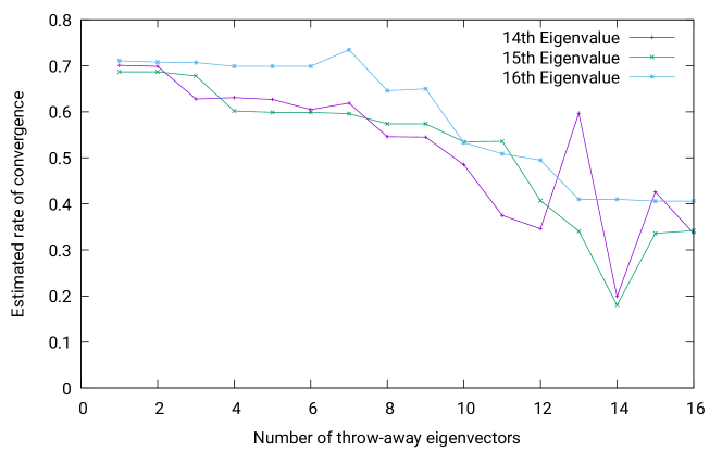
Figure 1: Experimentally-observed rates of convergence for the $14$th, $15$th, and $16$th non-zero eigenvalues depending on the number of throw-away eigenvectors

In our implementation, we use the preconditioned block inverse iteration and orthonormalize the iterates after every step. Figure 1 shows the results of an experiment with the permittivity

$$\epsilon(x) =\begin{cases}100&\text{ if }\|x-(1/2,1/2)\|\leq 1/3,\\ 1&\text{ otherwise}\end{cases} \text{ for all }x\in[0,1]\times[0,1],$$

where we aim to compute the first $16$ non-zero eigenvalues and add between $1$ and $16$ further “throw-away” eigenvectors to speed up convergence. We can see that the experimentally observed rate of convergence indeed is improved by adding more eigenvectors.

Of course, computing more eigenvectors increases the computational work (for $p\ll n$, we expect to need $\mathcal{O}(np^{2})$ operations), but our experiments indicate that the impact is more than compensated by the decrease in the number of required iteration steps if we base our stopping criterion only on the convergence of the relevant eigenvectors.

8 Numerical experiments

Since we can expect the eigenvalues to depend smoothly on the Bloch parameter, we can replace the entire Bloch parameter set $[-\pi/a,\pi/a]\times[-\pi/b,\pi/b]$ by a sufficiently fine equidistant grid. For our experiment, we choose $a=b=1$ and a grid with $30\times 30$ points

Maxwell’s equation is discretized on a coarse grid on the domain $[0,1]\times[0,1]$ with $16\times 16$ square elements on the coarsest mesh and $1024\times 1024$ square elements on the finest. On the finest mesh, we therefore have $2\,097\,152$ Nédélec basis functions.

We choose the piecewise constant permittivity function

$$\epsilon(x) =\begin{cases}11.56&\text{ if }\|x-(0.5,0.5)\|\leq 0.18,\\ 1&\text{ otherwise}\end{cases} \text{ for all }x\in[0,1]\times[0,1]$$

introduced by [7].

We compute the first $16$ eigenvalues using the block preconditioned inverse iteration. We stop the iteration as soon as the defects $\|Ae^{(m)}-Me^{(m)}\lambda_{m}\|_{2}$ of all eigenvector approximations drops below $10^{-2}$. Considering the scaling behaviour of the spectral norm as the grid is refined, this accuracy has been sufficient in our experiments.

In order to improve the rate of convergence, we compute $8$ additional “throw-away” eigenvector approximations, but they serve only to speed up convergence and to allow the algorithm to choose the approximations of the first $16$ eigenvectors from a $24$-dimensional space, they are not considered for the stopping criterion. The first and second eigenvalues depending on the Bloch parameter $k$ are displayed in fig. 2, the third and fourth in fig. 3. We observe that the eigenvalues change smoothly with the Bloch parameter. For all eigenvectors, the stopping criterion was reached, so the computed vectors are good approximations of the exact eigenvectors.

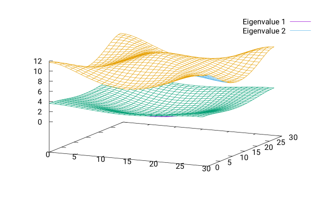
Figure 2: First and second eigenvalues depending on the Bloch parameter

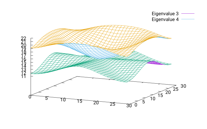
Figure 3: Third and fourth eigenvalues depending on the Bloch parameter

Of course, we are interested in the numerical performance of our method. Figure 4 shows the number of iterations required for the different Bloch values. We can see that our extrapolation method works very well: extrapolating between adjacent Bloch values to obtain an initial guess for the preconditioned inverse iteration reduces the number of required iteration steps to less than $4$ in most of the cases. Only close to the special case $k=0$ (in the four corners of the diagram), the algorithm requires a significantly increased number of steps.

Figure 4: Iterations required to obtain a residual norm below $10^{-2}$

References

• [1] D. N. Arnold, R. S. Falk, and R. Winther. Multigrid in $H(\mathop{\operatorname{div}})$ and $H(\mathop{\operatorname{curl}})$. Numer. Math., 85:197–217, 2000.
• [2] F. Bloch. Über die Quantenmechanik der Elektronen in Kristallgittern. Zeitschrift für Physik, 52(7):555–600, 1929.
• [3] J. H. Bramble, J. E. Pasciak, and A. V. Knyazev. A subspace preconditioning algorithm for eigenvector/eigenvalue computation. Adv. Comp. Math., 6:159–189, 1996.
• [4] R. Hiptmair. Multigrid method for Maxwell’s equations. SIAM J. Num. Anal., 36(1):204–225, 1998.
• [5] A. Knyazev. Toward the optimal preconditioned eigensolver: Locally optimal block preconditioned conjugate gradient method. SIAM J. Sci. Comp., 23(2):517–541, 2001.
• [6] A. V. Knyazev and K. Neymeyr. A geometric theory for preconditioned inverse iteration iii: A short and sharp convergence estimate for generalized eigenvalue problems. Lin. Alg. Appl, 358:95–114, 2003.
• [7] S. F. Mingaleev and Y. S. Kivshar. Nonlinear Localized Modes in 2D Photonic Crystals and Waveguides, volume 10 of Springer Series in Photonics, pages 351–369. Springer, 2003.
• [8] J. C. Nédélec. Mixed finite elements in $\mathbb{R}^{3}$. Num. Math., 35:315–341, 1980.
• [9] B. A. Samokish. The steepest descent method for an eigenvalue problem with semi-bounded operators. Izv. Vyssh. Uchebn. Zaved. Mat., 5:105–114, 1958. (in Russian).