All-optical magnetization control in CrI₃ monolayers: a microscopic theory

Abstract

Bright excitons in ferromagnetic monolayers CrI₃ efficiently interact with lattice magnetization, which makes all-optical resonant magnetization control possible in this material. Using the combination of ab-initio simulations within Bethe-Salpeter approach, semiconductor Bloch equations, and Landau-Lifshitz equations, we construct a microscopic theory of this effect. By solving numerically the resulting set of coupled equations describing the dynamics of atomic spins and spins of the excitons, we demonstrate the possibility of a tunable control of macroscopic magnetization of a sample.

I Introduction

Efficient control of the properties of layered structures is an important problem in both fundamental and applied research. In particular, a great demand exists for the development of optimal methods for control of magnetic characteristics of materials. This is not surprising, given the ever-increasing requirements for data-recording capacities of magnetic memory elements. The most important of them are compactness, energy efficiency, and recording speed. Regarding the latter, all-optical methods for the magnetic order manipulation look very promising as compared to traditional approaches based on the application of external magnetic field, as device operating frequencies can be enhanced by several orders of magnitude.

To date, there already exists a number of theoretical Gorchon et al. (2016); Moreno et al. (2017) and experimental works confirming the possibility of all-optical magnetization switching (AOMS) in a variety of magnetic compounds, including GdFeCo Ignatyeva et al. (2019); Aviles-Flix et al. (2020); Stanciu et al. (2007); Davies et al. (2020); Igarashi et al. (2020) and TbFeCo Lu et al. (2018) ferrimagnetic alloys, as well as in Pt/Co or Co/Gd multilayers El Hadri et al. (2016); van Hees et al. (2020).

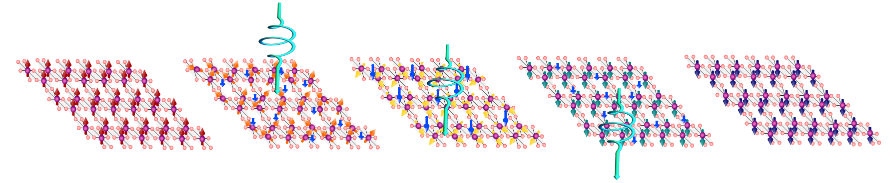
Figure 1: Schematic representation of the optical magnetization switching in CrI₃ monolayer. Here we demonstrate the system evolution in time (left to right). The monolayer is irradiated by circularly polarized light. Optical pumping leads to the formation of excitons carrying magnetic moment defined by the pump helicity which interact with the lattice magnetization of the sample.

Among all candidates where such a reorientation of magnetization is possible, materials combining ferromagnetic ordering with the presence of robust bright excitons are of particular interest Zhang et al. (2022). The examples of such materials are chromium trichalides, such as CrCl₃, CrBr₃ or CrI₃ Huang et al. (2018). In the present work, we take CrI₃ as an example, but the reported results should remain qualitatively the same for other members of the family. In the material we consider, the Cr³⁺ ions are arranged on the honeycomb lattice vertices surrounded by non-magnetic I^- ions McGuire et al. (2015). Being a 2D Ising ferromagnet, this material demonstrates robust optical excitonic response, with record high values of excitonic binding energies and oscillator strengths Wu et al. (2019), exceeding even the values reported for transition metal dichalcogenides Chernikov et al. (2014); Splendiani et al. (2010); Steinleitner et al. (2017); Wang et al. (2018).

The combination of such unique properties allowed some of us to propose that chromium trichalides were suitable candidates for polarization-sensitive resonant optical magnetization switching Kudlis et al. (2021), which was later on confirmed experimentally Zhang et al. (2022). The process of magnetic reorientation is connected with the transfer of angular momentum from excitons (electron-hole pairs) to the quasi-localized d-electrons of the Cr atoms, and corresponding phenomenological theory was developed in Ref. Kudlis et al., 2021. However, the full microscopic theory of the effect is still absent.

In this article, we make an attempt to construct such microscopic theory. We apply the well-established atomistic spin dynamics (ASD) formalism as basis of our work and couple it with the equations for the exciton dynamics by adding the terms describing the interaction between the spins of the excitons and the magnetic lattice. Numerical solution of the resulting set of equations allows us to analyze in detail the dynamics of the magnetization switching in real space and time.

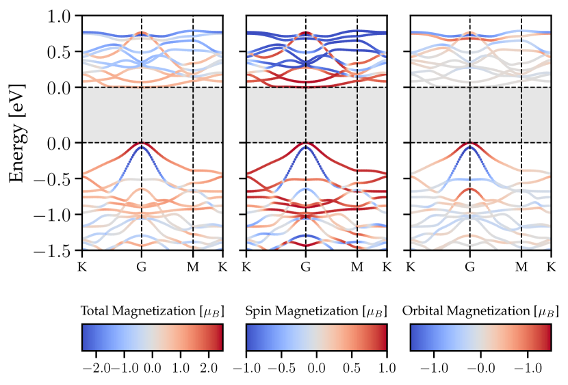
Figure 2: DFT band structure of excitons in CrI₃ monolayer with lattice constant $6.69$ Å. The color code shows total, spin, and orbital magnetization in the left, middle and right panel, respectively. The bandgap energy E=$2.59$ eV is indicated by gray shading. According to the first Brillouin zone grid, we have selected 16 valence bands and 14 conduction bands for the exciton basis.

The article is organized as follows. In Sec. II, we present calculations of the excitonic parameters in CrI₃, and then present the model Hamiltonian for coupled systems of excitons and lattice spins in Sec. III. Sec. IV presents the dynamic equations, and Sec. V contains the main results of the work, including the dependence of the switching properties on the parameters of the incident light beam. Sec. VI summarizes the results of the work.

II DFT/BSE calculations of exciton parameters for CrI₃

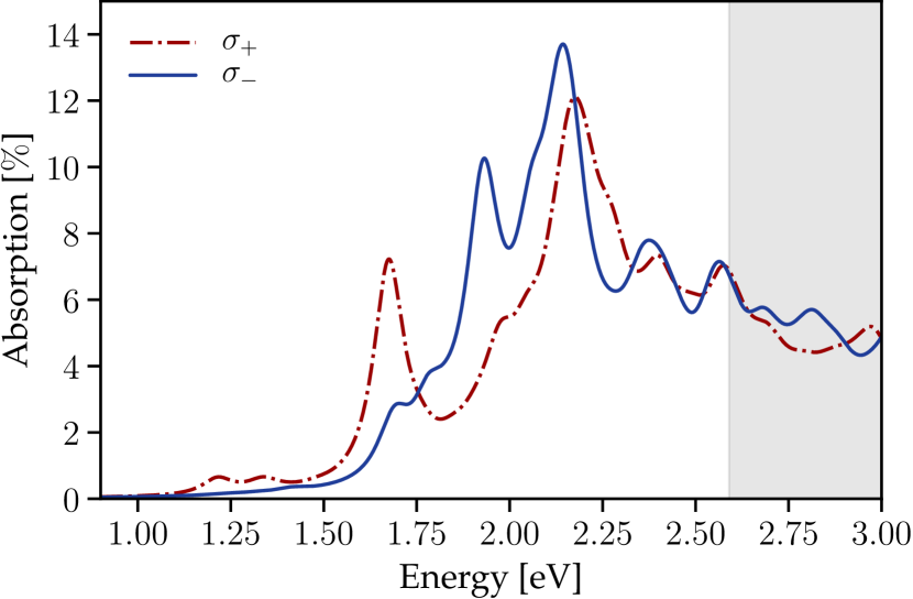
Figure 3: Absorption spectrum of CrI₃ sample for two circular polarizations. The solid line and the dashed line correspond to the $\sigma_{-}$ and $\sigma_{+}$ polarizations, respectively. The bandgap energy E=$2.59$ eV is indicated by gray shading.

We investigate the electronic structure of ferromagnetic CrI₃ monolayers via first-principles calculations employing density functional theory (DFT). The computations were executed using the GPAW package Mortensen et al. (2005a); Enkovaara et al. (2010). We use the cut-off energy of 600 eV for the plane-wave basis set and the LDA exchange-correlation functional incorporating spin-orbit effects Olsen (2016). To mitigate interaction between periodic images, 16 Å vacuum was used in the supercell.

Lattice constant for the CrI₃ ferromagnetic monolayer was determined via crystal lattice relaxation procedures, resulting in the value of $6.69$ Å. The force convergence criteria were set at 1 meV/Å per atom. To address the DFT bandgap issue, a scissor operator was employed to adjust the bandgap value to the experimental value of $2.59$ eV Wu et al. (2019).

The exciton spectrum was acquired utilizing the GPAW implementation of the Bethe-Salpeter equation Rohlfing and Louie (2000); Yan et al. (2011); Hüser et al. (2013); Olsen (2021). Screened Coulomb potential expressions were derived with the dielectric cutoff of 50 eV, 200 electronic bands, and a 2D truncated Coulomb potential Hüser et al. (2013). The exciton basis was configured with 16 valence bands and 14 conduction bands on a 6$\times$6 grid of the first Brillouin zone.

In Fig. 2, we demonstrate the band structure of the CrI₃ monolayer with color bars for the orbital, spin and total magnetization which are shown below the main figures. The bandgap of $2.59$ eV is highlighted by the gray area. The analysis of the polarization-resolved absorption spectrum of the CrI₃ monolayer is shown in Fig. 3. As one can see, there is a remarkable difference in the absorption of the $\sigma_{+}$ and $\sigma_{-}$ components. The prominent absorption peaks in both absorption profiles are related to the excitonic transitions. Naturally, if the magnetization of the sample is inverted, the absorption curves corresponding to opposite polarizations interchange. This forms the basis of the magnetization switching mechanism: for a given pump frequency and polarization, the magnetic sublattice tends to orient its magnetization so as to maximize the absorption Kudlis et al. (2021).

III The model Hamiltonian

The total energy $E$ of the system includes three terms:

$$E=E_{\text{m}}+E_{\text{exc}}+E_{\text{s}},$$ (1)

describing the contributions from the magnetic subsystem, excitonic subsystem, and the interaction between them. The magnetic structure of the CrI₃ monolayer is described within the model of classical spin vectors localized on sites of the honeycomb lattice of the Cr atoms. The corresponding energy is given by:

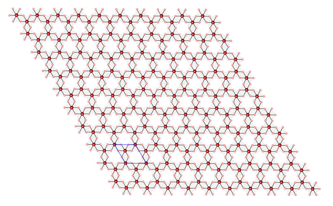
Figure 4: CrI₃ structure. The atoms of chromium and iodine are represented by red and pink spheres, respectively. The unit cell of CrI₃ consists of two Cr atoms and six I atoms, with the Cr atoms forming a honeycomb structure.

$$E_{\textup{m}}=-J\sum_{<i,j>}\boldsymbol{m}_{i}\cdot\boldsymbol{m}_{j}-D\sum_{<i,j>}\boldsymbol{d}_{ij}\cdot\left[\boldsymbol{m}_{i}\times\boldsymbol{m}_{j}\right]\\ -K\sum_{i}\left(\boldsymbol{m}_{i}\cdot\boldsymbol{e}_{z}\right)^{2}-\mu\sum_{i}\boldsymbol{B}\cdot\boldsymbol{m}_{i}.$$ (2)

Here, the first, second, third, and fourth terms describe the Heisenberg exchange, the Dzyaloshinskii–Moriya interaction (DMI), the uniaxial magnetocrystalline anisotropy and the Zeeman interaction, respectively; $\boldsymbol{m}_{i}$ is the unit vector pointing along the $i$th magnetic moment, whose magnitude is $\mu$ for each lattice site; $\boldsymbol{B}$ is the external magnetic field, and $\boldsymbol{d}_{ij}=\boldsymbol{r}_{ij}\times\boldsymbol{e}_{z}/|\boldsymbol{r}_{ij}|$ is the DMI unit vector with $\boldsymbol{e}_{z}$ and $\boldsymbol{r}_{ij}$ being the unit vector along the monolayer normal and the vector pointing from site $i$ to site $j$, respectively. The angular brackets indicate summation over unique nearest neighbors only. The effective parameter values are taken from Ref. Ghosh et al. (2020): $J=2.53$ meV, $D=1.2$ meV, $K=0.153$ meV, and $\mu=3.0~{}\mu_{B}$. The external magnetic field is in the monolayer plane, with the magnitude ranging from 0 T to 3.5 T. In our calculations, we use the computational domain of $N_{\textup{c}}=30\times 30=900$ unit cells equipped with periodic boundary conditions. Note that the number of magnetic moments $N_{\textup{a}}$ explicitly included in the calculations is twice as large as $N_{c}$.

The Hamiltonian describing the excitonic subsystem reads:

$$H_{\text{exc}}=\sum_{\textbf{q}n}E_{n\textbf{q}}\hat{X}^{\dagger}_{n\textbf{q}}\hat{X}_{n\textbf{q}}\\ +\boldsymbol{E}_{\pm}\sum_{n}\boldsymbol{D}_{n\textbf{q}=0}\hat{X}^{\dagger}_{0\textbf{q}=0}\hat{X}_{n\textbf{k}=0}+h.c.$$ (3)

Here, $\hat{X}^{\dagger}_{n\textbf{q}}$ ($\hat{X}_{n\textbf{q}}$) are the exciton creation (annihilation) operators characterized by momentum $\boldsymbol{q}$ and state $n$ labeling the peak in the absorption spectrum, $E_{n\textbf{q}}$ is the exciton energy, $\boldsymbol{D}_{n\textbf{q}=0}$ is the dipole moment of the optical transition obtained from the DFT calculations (see Appendix A), here limited to the direct-gap transitions, $\boldsymbol{E}_{\pm}(t)=\text{Re}\left[(E_{0},\mp\textup{i}E_{0},0)exp(-\textup{i}\omega t)\right]h(t)$ is the right- or left-circularly polarized electric field characterized by the pulse envelope $h(t)$. The effects of both radiative and non-radiative damping are described phenomenologically, see Appendix B for details.

The interaction between the excitonic and magnetic subsystems is characterized by the following Hamiltonian:

$$H_{\text{s}}=-g\mu\!\!\!\sum_{\begin{subarray}{c}\textbf{q}\textbf{q}^{\prime}nn^{\prime}\end{subarray}}\!\!\!\left(\boldsymbol{m}_{\textbf{q}-\textbf{q}^{\prime}}-\boldsymbol{m}^{\text{g}}_{\textbf{q}-\textbf{q}^{\prime}}\right)\boldsymbol{M}^{\textbf{q}\textbf{q}^{\prime}}_{nn^{\prime}}\hat{X}^{\dagger}_{n\textbf{q}}\hat{X}_{n^{\prime}\textbf{q}^{\prime}},$$ (4)

where the term inside the parentheses is the Fourier transform of the magnetization relative to the collinear ground state (see Appendix C), $\boldsymbol{M}^{\textbf{q}\textbf{q}^{\prime}}_{nn^{\prime}}$ is the dipole matrix element describing the interaction with local magnetic moment, $g$ is the on-site spin-exciton coupling constant (see Appendix A for the details). The evaluation of the coupling constant $g$ can not be performed using standard DFT approaches and requires a separate consideration which goes beyond the scope of the present work. Here, $g$ is taken as a phenomenological parameter with the value $g=2.3$ meV, which is slightly less then the exchange interaction parameter in the magnetic lattice Hamiltonian.

Note that exciton-exciton interaction is neglected and only single exciton wavefunction $\Psi_{\text{exc}}$ is considered explicitly. Therefore:

$$E_{\text{s}}\approx n_{\textup{exc}}\braket{\Psi_{\text{exc}}}{H_{\text{s}}}{\Psi_{\text{exc}}}=-g\mu\sum\limits_{i}\boldsymbol{\sigma}_{i}(\boldsymbol{m}_{i}-\boldsymbol{m}_{i}^{\textup{g}}).$$ (5)

Here, $n_{\textup{exc}}$ is the scaling factor proportional to the number of the unit cells (in our case $n_{\text{exc}}=450$), $\boldsymbol{m}^{\textup{g}}\equiv\boldsymbol{e}_{z}$ is the unit vector along the ground-state magnetization, $\boldsymbol{\sigma}_{i}$ is the exciton spin vector associated with the $i$th unit cell (note that excitons in CrI₃ are of the Frenkel type) defined via the following equation:

$$\boldsymbol{\sigma}_{i}=n_{\text{exc}}\sum_{\textbf{q}\textbf{q}^{\prime}}e^{2\pi\textup{i}(\boldsymbol{r}_{i}(\boldsymbol{q}^{\prime}-\boldsymbol{q}))_{N_{\textup{c}}}}\sum_{nn^{\prime}}C_{n}^{\textbf{q}*}\boldsymbol{M}^{\textbf{q}\textbf{q}^{\prime}}_{nn^{\prime}}C_{n^{\prime}}^{\textbf{q}^{\prime}},$$ (6)

where $\boldsymbol{r}_{i}$ is the position of $i$th unit cell and $C_{n}^{\textbf{q}}$ are the expansion coefficients of $\Psi_{\text{exc}}$:

$$\Psi_{\text{exc}}=\sum_{n\textbf{q}}C_{n}^{\textbf{q}}\hat{X}^{\dagger}_{n\textbf{q}}|0\rangle.$$ (7)

IV Dynamic equations

The dynamic equations for the observables follow from the model Hamiltonian. The evolution of $\Psi_{\text{exc}}$ is accessed via the equation of motion for its coefficients:

$$i\hbar\frac{\partial C_{n}^{\textbf{q}}}{\partial t}=\sum_{n^{\prime}\textbf{q}^{\prime}}H_{nn^{\prime}}^{\textbf{q}\textbf{q}^{\prime}}(t)C_{n^{\prime}}^{\textbf{q}^{\prime}}(t),$$ (8)

where $H_{nn^{\prime}}^{\textbf{q}\textbf{q}^{\prime}}$ are the matrix elements of the excitonic Hamiltonian $H=H_{\textup{exc}}+H_{\textup{s}}$.

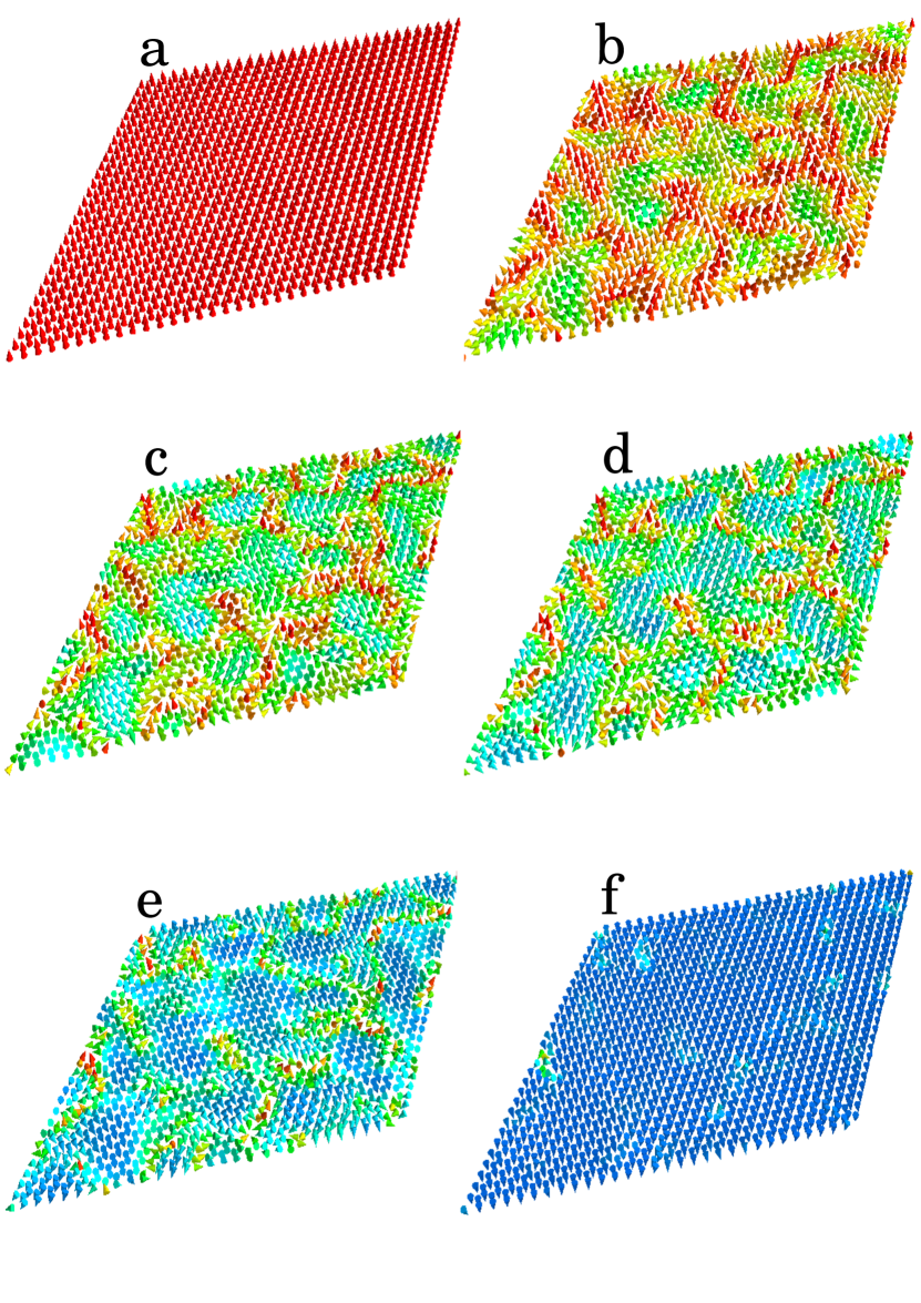
Figure 5: Evolution of the magnetic structure of the system for the pulse fluence $F_{1}=166$ mJ/cm². The fluence magnitude is sufficient to induce the magnetization reversal. The snapshots (a)-(f) correspond to $1.6$ ps, $1.8$ ps, $1.84$ ps, $1.86$ ps, $1.9$ ps, and $2.04$ ps, respectively. The color codes the orientation of the magnetic moments of the Cr atoms.

This case corresponds to the solid line in Fig. 7.

On the other hand, the dynamics of the lattice magnetization is obtained via the time integration of the Landau-Lifshitz-Gilbert equation (LLGE) for the normalized magnetization vectors at zero temperature:

$$\dfrac{d\boldsymbol{m}_{i}}{dt}=-\gamma\boldsymbol{m}_{i}\times\boldsymbol{B}^{\text{eff}}_{i}+\eta\left(\boldsymbol{m}_{i}\times\dfrac{d\boldsymbol{m_{i}}}{dt}\right),$$ (9)

where $\gamma$ is the gyromagnetic ratio, $\eta$ is the dimensionless damping parameter (in the present study we take $\eta=0.2$), and $\boldsymbol{B}^{\text{eff}}_{i}$ is the effective magnetic field defined as:

$$\boldsymbol{B}^{\text{eff}}_{i}=-\frac{1}{\mu}\frac{\partial E}{\partial\boldsymbol{m}_{i}}.$$ (10)

Note that only $E_{\text{m}}+E_{\text{s}}$ depends explicitly on $\boldsymbol{m}_{i}$. The effect of excitons on the magnetization dynamics is treated within the mean-field approach, where the magnetization-exciton interaction energy $E_{\text{s}}$ depends on the exciton spin vector configuration $\boldsymbol{\sigma}$ [see Eq. (5)], which needs to be updated every time step using Eqs. (8) and (6). We use the semi-implicit solver by Mentink et al. Mentink et al. (2010) for the time integration of the LLGE.

V Results and discussion

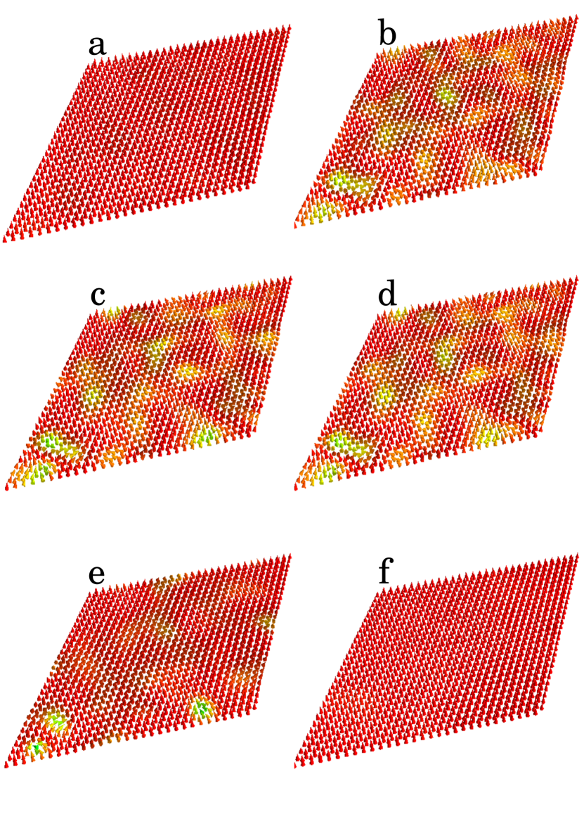
Figure 6: Evolution of the magnetic structure of the system for the pulse fluence $F_{2}=33$ mJ/cm². The fluence magnitude is insufficient to induce the magnetization reversal. The snapshots (a)-(f) correspond to $2.2$ ps, $2.76$ ps, $2.98$ ps, $3.2$ ps, $4.4$ ps, and $8.0$ ps, respectively. The color codes the orientation of the magnetic moments of the Cr atoms. This case corresponds to the dashed line in Fig. 7.

We study the dynamics of the system induced by spatially homogeneous circular polarized laser pulse at normal incidence. The choice of the pulse envelope $h(t)$ is inspired by real setups Maciej et al. (2022); Zhang et al. (2022):

$$h(t)=A\theta(t_{f}-|2t-t_{f}|)\exp{\left[-B\left(\dfrac{t-t_{f}/2}{t_{f}}\right)^{2}\right]}.$$ (11)

Here $t_{\text{f}}$ is the duration of the pulse, and $A=1.94$ and $B=32.2$ are dimensionless parameters defining the total pulse fluence $F$:

$$F =\dfrac{E_{0}^{2}c\varepsilon_{0}}{2}\int\limits_{0}^{t_{f}}h(t)^{2}dt=CI_{0}t_{f},$$ (12)

where $I_{0}=E_{0}^{2}c\varepsilon_{0}$ is the intensity of the pulse and $C=A^{2}\text{erf}(\sqrt{B/2})\sqrt{\pi/(2B)}$ is the dimensionless constant. In our calculations, the intensity never exceeds the value of 0.1 TW/cm², which is consistent with experiments Maciej et al. (2022); Zhang et al. (2022). We take the duration of the pulse $t_{f}=4$ ps and its central frequency $\omega=1.94$ eV, which is below the direct bandgap. Note that the chosen value of $\omega$ is in the vicinity of one of the $\sigma^{-}$ peaks in the absorption spectrum.

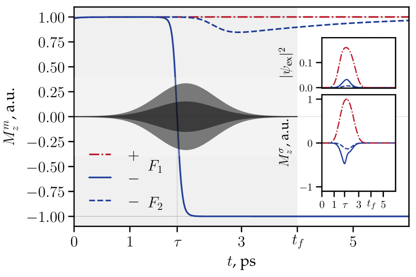
Figure 7: Time-dependence of the cumulative out-of-plane magnetization $M_{z}^{m}$ for different light polarizations. Shaded area indicates the laser pulse duration. Upper right inset shows the time dependence of $|\psi_{ex}|^{2}=|\Psi_{\text{exc}}|^{2}-|\psi_{0}|^{2}$ describing the evolution of excited exciton states. Lower right inset shows the time dependence of the exciton magnetization. Dark grey areas show the envelope functions for the optical pump pulse with fluence $F_{1}=166$ mJ/cm² (lighter grey, magnetization reversal occurs) and $F_{2}=33.2$ mJ/cm² (darker grey, magnetization reversal does not occur). The switching time $\tau$ is defined by the instant when $M_{z}^{m}$ changes sign. Here $\tau=1.85$ ps. The signs $+$ and $-$ correspond to right-hand and left-hand circularly polarized light, respectively.

The initial magnetization direction is prepared by aligning all magnetic vectors along $\boldsymbol{e}_{z}$ and perturbing them by small random noise to break the symmetry. The simulation of the spatio-temporal magnetization pattern provides information about the evolution of the cumulative out-of-plane magnetization due to the spin lattice and excitons:

$$M_{z}^{m}(t)=\dfrac{1}{N_{\textup{a}}}\sum\limits_{i=1}^{N_{\textup{a}}}m_{i}^{z}(t),\quad M_{z}^{\sigma}(t)=\dfrac{1}{N_{\textup{c}}}\sum\limits_{i=1}^{N_{\textup{c}}}\sigma_{i}^{z}(t),$$ (13)

The dynamics of the magnetization switching is shown in Fig.5. The arrival of the pulse with $\sigma^{-}$ polarization leads to the appearance of the randomly distributed domains with inverted magnetization. This process is accompanied by the formation of magnetic vortices favored by the DMI. If the fluence exceeds some critical value $F_{c}$, the size of the domains increases with time, making the system eventually reach the state with spatially homogeneous inverted magnetization (see Fig. 5). On the other hand, if the fluence is below the critical value, the system relaxes back to the homogeneous state without magnetization inversion (see Fig. 6)).

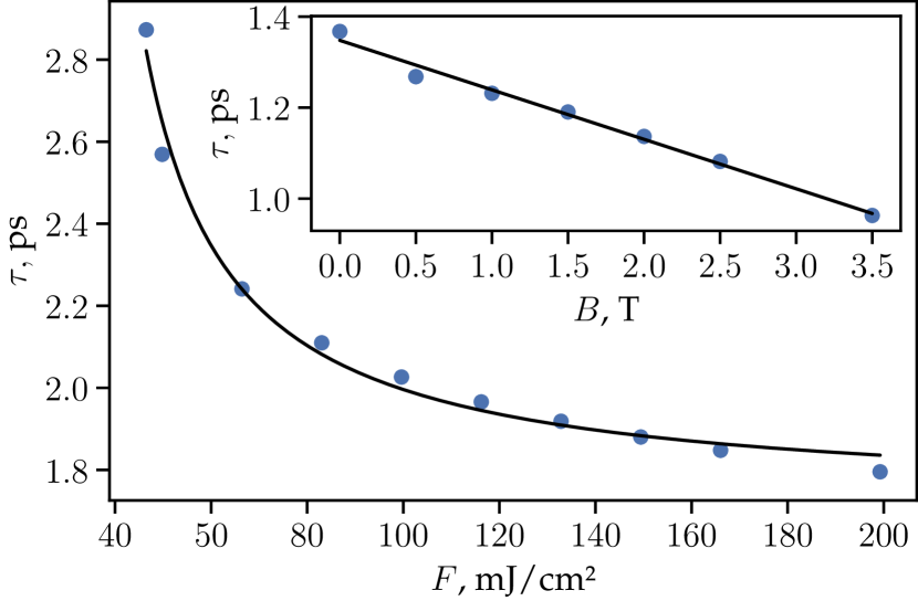
Figure 8: Magnetization switching time $\tau$ as a function of pump fluence $F$. Magnetization switching is achieved if the fluence of the pulse exceeds a critical value $F_{c}\approx 46$ mJ/cm², at which the switching time diverges. The inset shows the switching time as a function of the lateral external magnetic field for the fluence of $133$ mJ/cm².

The dynamics of the cumulative magnetization is shown in Fig. 7. The transition between up and down polarized states induced by the pulse is quite abrupt, which makes it possible to introduce the characteristic switching time $\tau$ – the principal parameter characterizing the magnetization reversal. As expected, $\tau$ decreases with increasing $F$ (see Fig. 8). The switching time becomes infinite when the fluence reaches the critical value $F_{c}\approx 46$ mJ/cm², below which no magnetization reversal is possible. This behavior agrees well with our previous study based on the phenomenological model of resonant magnetization switching Kudlis et al. (2021). Interestingly, the switching time is influenced by lateral magnetic field (see inset in Fig. 8).

The change of the circular polarization of the incident beam modifies drastically the magnetization dynamics: the switching does not occur for the initial magnetization pointing up, but can happen for the initial magnetization pointing down.

VI Conclusion

In conclusion, we developed a microscopic theory of all-optical resonant polarization-sensitive magnetization switching in monolayers of CrI₃. The effect is due to the combination of the peculiar optical selection rules for excitons in this material and efficient coupling of excitons to the magnetic lattice. The spatio-temporal distribution of the magnetization under circular polarized pulses was investigated, and the dependence of the parameters characterizing the switching on the properties of the optical pulse was determined.

Appendix A Matrix elements of the exciton Hamiltonian

The matrix elements of the exciton Hamiltonian $H_{\text{exc}}+H_{\text{s}}$ are computed via the resolution of the Bethe-Salpeter equation (BSE) parameterized using the first-principles calculations. The exciton wave functions and associated energies are obtained by diagonalizing the BSE Hamiltonian Onida et al. (2002); Rohlfing and Louie (2000, 1998) as follows:

$$\sum_{c^{\prime}v^{\prime}\textbf{k}^{\prime}}H^{BSE}_{cv\textbf{k}c^{\prime}v^{\prime}\textbf{k}^{\prime}}(\textbf{q})A^{n\textbf{q}}_{c^{\prime}v^{\prime}\textbf{k}^{\prime}}=E^{n\textbf{q}}A^{n\textbf{q}}_{cv\textbf{q}},$$ (14)

Here, $H^{BSE}_{cv\textbf{k}c^{\prime}v^{\prime}\textbf{k}^{\prime}}(\textbf{q})$ are the matrix elements of the BSE Hamiltonian for excitons possessing momentum q, $A^{n\textbf{q}}_{cv\textbf{q}}$ and $E^{n\textbf{q}}$ are the $n$th exciton wave function and energy, respectively. The indices $c$ ($c^{\prime}$), $v$ ($v^{\prime}$), and k ($\textbf{k}^{\prime}$) denote the conduction band, valence band, and single-particle momentum, respectively. The Hamiltonian $H^{BSE}$ is calculated using the Tamm-Dancoff approximation Onida et al. (2002), which is particularly well-suited for wide-gap semiconductors. This approximation disregards the coupling between resonance and anti-resonance poles while preserving the Hermitian character of the Hamiltonian.

The calculation of the dipole matrix elements is carried out utilizing the following equation:

$$\boldsymbol{D}_{n\textbf{q}=0}=\langle 0|\boldsymbol{r}|n\textbf{q}=0\rangle=\sum_{cv\textbf{k}}A^{n\textbf{q}=0}_{cv\textbf{k}}\langle v\textbf{k}|\boldsymbol{r}|c\textbf{k}\rangle,$$ (15)

where $\langle v\textbf{k}|\boldsymbol{r}|c\textbf{k}\rangle$ is the single-particle dipole matrix element corresponding to the optical transition from the conduction band $c$ to the valence band $v$ with momentum k.

The key ingredients of the exciton-skyrmion Hamiltonian interaction are the matrix elements of the exciton magnetic moment $\boldsymbol{M}^{\textbf{q}\textbf{q}^{\prime}}_{nn^{\prime}}$. These matrix elements are assembled from the matrix elements of the spin magnetic moment $\boldsymbol{S}^{\textbf{q}\textbf{q}^{\prime}}_{nn^{\prime}}$ and the orbital magnetic moment $\boldsymbol{L}^{\textbf{q}\textbf{q}^{\prime}}_{nn^{\prime}}$. The matrix elements of the spin magnetic moment are calculated from the single-particle spin moment:

$$\boldsymbol{S}^{\textbf{q}\textbf{q}^{\prime}}_{nn^{\prime}}= \sum_{cv\textbf{k},c^{\prime}v^{\prime}\textbf{k}^{\prime}}\left(A^{n\textbf{q}}_{cv\textbf{k}}\right)^{*}A^{n^{\prime}\textbf{q}^{\prime}}_{c^{\prime}v^{\prime}\textbf{k}^{\prime}}$$

$$\times\left[\langle c\textbf{k+q}|\boldsymbol{S}|c^{\prime}\textbf{k}^{\prime}+\textbf{q}^{\prime}\rangle-\langle v^{\prime}\textbf{k}^{\prime}|\boldsymbol{S}|v\textbf{k}\rangle\right],$$ (16)

where $\langle c\textbf{k}|\boldsymbol{S}|c^{\prime}\textbf{k}^{\prime}\rangle$ is the single-particle spin matrix element. While the single-particle spin operators are simply defined using the Pauli matrices in the spin subspace, the calculation of the orbital moment requires a more careful consideration. In our study, we employ a local projector augmented wave (PAW) technique to evaluate the orbital single-particle magnetic moment, as it offers a more straightforward approach compared to the previously reported perturbation theory-based methods Deilmann et al. (2020); Woźniak et al. (2020); Lopez et al. (2012); Thonhauser et al. (2005); Ceresoli et al. (2006). All-electron orbitals inside the PAW sphere can be expanded as Mortensen et al. (2005b); Blöchl (1994)

$$|c\textbf{k}\rangle=\sum_{i}\langle p_{i}^{a}|\varphi_{c\textbf{k}}\rangle|\phi_{i}^{a}\rangle,$$ (17)

where $p_{i}^{a}$ is a projector of the smooth pseudowave function $\varphi_{c\textbf{k}}$ for band $c$ with momentum k on the $i{\text{th}}$ all-electron partial wave for atom $a$, $\phi_{i}^{a}$. We calculate the one-particle matrix elements of the orbital momentum as follows Olsen (2016):

$$\langle c\textbf{k}|\boldsymbol{L}|c^{\prime}\textbf{k}^{\prime}\rangle=\sum_{ai_{1}i_{2}}\langle\varphi_{c\textbf{k}}|p_{i_{1}}^{a}\rangle\langle\phi_{i1}^{a}|\boldsymbol{L}^{a}|\phi_{i2}^{a}\rangle\langle p_{i_{2}}^{a}|\varphi_{c^{\prime}\textbf{k}^{\prime}}\rangle,$$ (18)

where $\boldsymbol{L}^{a}$ is the orbital momentum operator for atom $a$. Since partial waves $\phi_{i}^{a}$ are usually defined in a spherical basis, the matrix elements $\langle\phi_{i1}^{a}|\boldsymbol{L}^{a}|\phi_{i2}^{a}\rangle$ can be calculated analytically. Having single-particle matrix elements of the orbital magnetic moment, we compute the exciton matrix elements as follows:

$$\boldsymbol{L}^{\textbf{q}\textbf{q}^{\prime}}_{nn^{\prime}} =\sum_{cv\textbf{k},c^{\prime}v^{\prime}\textbf{k}^{\prime}}\left(A^{n\textbf{q}}_{cv\textbf{k}}\right)^{*}A^{n^{\prime}\textbf{q}^{\prime}}_{c^{\prime}v^{\prime}\textbf{k}^{\prime}}$$

$$\quad\times\left[\langle c\textbf{k+q}|\boldsymbol{L}|c^{\prime}\textbf{k}^{\prime}+\textbf{q}^{\prime}\rangle-\langle v^{\prime}\textbf{k}^{\prime}|\boldsymbol{L}|v\textbf{k}\rangle\right].$$ (19)

The total exciton magnetic moment is obtained by computing a sum of the spin and orbital components:

$$\boldsymbol{M}^{\textbf{q}\textbf{q}^{\prime}}_{nn^{\prime}}=\boldsymbol{L}^{\textbf{q}\textbf{q}^{\prime}}_{nn^{\prime}}+\boldsymbol{S}^{\textbf{q}\textbf{q}^{\prime}}_{nn^{\prime}}.$$ (20)

Appendix B Introduction of damping

The effects of damping are modeled by introducing finite inverse relaxation time $\delta$, which results in the decay of excited exitonic states $\sim\exp(-\Delta t\delta)$ with time $\Delta t$. For simplicity, the damping parameter is assumed to be the same for all excited excitonic states. Therefore, at each time step of the simulation, the vector of state $\Psi_{\text{exc}}=(\psi_{0},\psi_{1},\dots,\psi_{n})$ with $\psi_{0}$ being the component responsible for vacuum, is substituted by the modified vector of state $\Psi_{\text{exc}}\leftarrow\tilde{\Psi}_{\text{exc}}=(\tilde{\psi}_{0},\tilde{\psi}_{1},\dots,\tilde{\psi}_{n})$, whose componens are defined via the following operations:

$$\tilde{\psi}_{i}=\psi_{i}\sqrt{1-\Delta t\delta},\text{}i>0$$ (21)

$$\Delta=1-\left(\sum\limits_{i=1}^{n}|\tilde{\psi}_{i}|^{2}+|\psi_{0}|^{2}\right),$$ (22)

$$\tilde{\psi}_{0}=\psi_{0}\dfrac{\sqrt{\Delta+|\psi_{0}|^{2}}}{|\psi_{0}|}.$$ (23)

Note that $|\tilde{\Psi}_{\text{exc}}|=|\Psi_{\text{exc}}|=1$. In our study, we take $\delta=80$ meV.

Appendix C Fourier transforms

The definition of the direct and inverse Fourier transforms used in this study requires a special discussion since the gratings in the real space(r) and momentum space(q) have different discreteness. For an arbitrary function $f$, the Fourier transforms are defined via the following equations:

$$f(\boldsymbol{r}_{i})= \sum\limits_{j}^{N_{q}}\exp\left[2\pi\text{i}(\boldsymbol{r}_{i}\boldsymbol{q}_{j})_{N_{c}}\right]f(\boldsymbol{q}_{j}),$$ (24)

$$f(\boldsymbol{q}_{j})= \dfrac{1}{N_{c}}\sum\limits_{i}^{N_{\textup{c}}}\exp\left[-2\pi\text{i}(\boldsymbol{r}_{i}\boldsymbol{q}_{j})_{N_{c}}\right]f(\boldsymbol{r}_{i}),$$ (25)

where $N_{\textup{c}}=30\times 30=900$ is the number of unit cells and $N_{q}=6\times 6=36$ is the number of points in the $q$-space. We define the dot product $(\dots)_{N_{c}}$ as:

$$(\boldsymbol{r}\boldsymbol{q})_{N_{c}}=\frac{r^{x}_{i}q^{x}_{j}}{N^{x}_{c}}+\frac{r^{y}_{i}q^{y}_{j}}{N^{y}_{c}}+\frac{r^{z}_{i}q^{z}_{j}}{N^{z}_{c}}.$$ (26)

We use $N^{x}_{\textup{c}}=N^{y}_{\textup{c}}=30$ and $N^{z}_{\textup{c}}=1$. Since there are two magnetic atoms per unit cell, we adhere to the following formula to compute the Fourier transform of the magnetization:

$$\boldsymbol{m}_{\textbf{q}-\textbf{q}^{\prime}}=\dfrac{1}{N_{c}}\sum\limits_{i}^{N_{\textup{c}}}\exp\left[-2\pi\text{i}(\boldsymbol{r}_{i}\left(\textbf{q}-\textbf{q}^{\prime}\right))_{N_{c}}\right]$$ (27)

$$\qquad\qquad\qquad\qquad\qquad\qquad\times(\boldsymbol{m}_{2i}+\boldsymbol{m}_{2i-1}),$$

where we use the total magnetic moment of the unit cell.

References

- Gorchon et al. (2016) J. Gorchon, R. B. Wilson, Y. Yang, A. Pattabi, J. Y. Chen, L. He, J. P. Wang, M. Li, and J. Bokor, “Role of electron and phonon temperatures in the helicity-independent all-optical switching of gdfeco,” Phys. Rev. B 94, 184406 (2016).
- Moreno et al. (2017) R. Moreno, T. A. Ostler, R. W. Chantrell, and O. Chubykalo-Fesenko, “Conditions for thermally induced all-optical switching in ferrimagnetic alloys: Modeling of tbco,” Phys. Rev. B 96, 014409 (2017).
- Ignatyeva et al. (2019) D. O. Ignatyeva, C. S. Davies, D. A. Sylgacheva, A. Tsukamoto, H. Yoshikawa, P. O. Kapralov, A. Kirilyuk, V. I. Belotelov, and A. V. Kimel, “Plasmonic layer-selective all-optical switching of magnetization with nanometer resolution,” Nature Comm. 10, 4786 (2019).
- Aviles-Flix et al. (2020) L. Aviles-Flix, A. Olivier, G. Li, C. S. Davies, L. Alvaro-Gomez, M. Rubio-Roy, S. Auffret, A. Kirilyuk, A. V. Kimel, Th. Rasing, L. D. Buda-Prejbeanu, R. C. Sousa, B. Dieny, and I. L. Prejbeanu, “Single-shot all-optical switching of magnetization in tb/co multilayer-based electrodes,” Sci. Rep. 10, 5211 (2020).
- Stanciu et al. (2007) C. D. Stanciu, F. Hansteen, A. V. Kimel, A. Kirilyuk, A. Tsukamoto, A. Itoh, and Th. Rasing, “All-optical magnetic recording with circularly polarized light,” Phys. Rev. Lett. 99, 047601 (2007).
- Davies et al. (2020) C. S. Davies, T. Janssen, J. H. Mentink, A. Tsukamoto, A. V. Kimel, A. F. G. van der Meer, A. Stupakiewicz, and A. Kirilyuk, “Pathways for single-shot all-optical switching of magnetization in ferrimagnets,” Phys. Rev. Applied 13, 024064 (2020).
- Igarashi et al. (2020) J. Igarashi, Q. Remy, S. Iihama, G. Malinowski, M. Hehn, J. Gorchon, J. Hohlfeld, S. Fukami, H. Ohno, and S. Mangin, “Engineering single-shot all-optical switching of ferromagnetic materials,” Nano Lett. 20, 8654 (2020).
- Lu et al. (2018) X. Lu, X. Zou, D. Hinzke, T. Liu, Y. Wang, T. Cheng, J. Wu, T. A. Ostler, J. Cai, U. Nowak, R. W. Chantrell, Y. Zhai, and Y. Xu, “Roles of heating and helicity in ultrafast all-optical magnetization switching in tbfeco,” Appl. Phys. Lett. 113, 032405 (2018).
- El Hadri et al. (2016) M. S. El Hadri, P. Pirro, C.-H. Lambert, S. Petit-Watelot, Y. Quessab, M. Hehn, F. Montaigne, G. Malinowski, and S. Mangin, “Two types of all-optical magnetization switching mechanisms using femtosecond laser pulses,” Phys. Rev. B 94, 064412 (2016).
- van Hees et al. (2020) Y. L. W. van Hees, P. van de Meugheuvel, B. Koopmans, and R. Lavrijsen, “Deterministic all-optical magnetization writing facilitated by non-local transfer of spin angular momentum,” Nature Comm. 11, 3835 (2020).
- Zhang et al. (2022) Peiyao Zhang, Ting-Fung Chung, Quanwei Li, Siqi Wang, Qingjun Wang, Warren L. B. Huey, Sui Yang, Joshua E. Goldberger, Jie Yao, and Xiang Zhang, “All-optical switching of magnetization in atomically thin CrI3,” Nature Materials 21, 1373–1378 (2022).
- Huang et al. (2018) Bevin Huang, Genevieve Clark, Dahlia R Klein, David MacNeill, Efrén Navarro-Moratalla, Kyle L Seyler, Nathan Wilson, Michael A McGuire, David H Cobden, Di Xiao, et al., “Electrical control of 2d magnetism in bilayer cri3,” Nature nanotechnology 13, 544–548 (2018).
- McGuire et al. (2015) Michael A McGuire, Hemant Dixit, Valentino R Cooper, and Brian C Sales, “Coupling of crystal structure and magnetism in the layered, ferromagnetic insulator cri3,” Chemistry of Materials 27, 612–620 (2015).
- Wu et al. (2019) M. Wu, Z. Li, T. Cao, and S. G. Louie, “Physical origin of giant excitonic and magneto-optical responses in two-dimensional ferromagnetic insulators,” Nature Comm. 10, 2371 (2019).
- Chernikov et al. (2014) A. Chernikov, T. C. Berkelbach, H. M. Hill, A. Rigosi, Y. Li, O. B. Aslan, D. R. Reichman, M. S. Hybertsen, and T. F. Heinz, “Exciton binding energy and nonhydrogenic rydberg series in monolayer ,” Phys. Rev. Lett. 113, 076802 (2014).
- Splendiani et al. (2010) A. Splendiani, L. Sun, Y. Zhang, T. Li, J. Kim, C.-Y. Chim, G. Galli, and F. Wang, “Emerging photoluminescence in monolayer ,” Nano Lett. 10, 1271 (2010).
- Steinleitner et al. (2017) P. Steinleitner, P. Merkl, P. Nagler, J. Mornhinweg, C. Schüller, T. Korn, A. Chernikov, and R. Huber, “Direct observation of ultrafast exciton formation in a monolayer of ,” Nano Lett. 17, 1455 (2017).
- Wang et al. (2018) G. Wang, A. Chernikov, M. M. Glazov, T. F. Heinz, X. Marie, T. Amand, and B. Urbaszek, “Colloquium: Excitons in atomically thin transition metal dichalcogenides,” Rev. Mod. Phys. 90, 021001 (2018).
- Kudlis et al. (2021) A. Kudlis, I. Iorsh, and I. A. Shelykh, “All-optical resonant magnetization switching in monolayers,” Phys. Rev. B 104, L020412 (2021).
- Mortensen et al. (2005a) J. J. Mortensen, L. B. Hansen, and K. W. Jacobsen, “Real-space grid implementation of the projector augmented wave method,” Physical Review B 71 (2005a), 10.1103/physrevb.71.035109.
- Enkovaara et al. (2010) J Enkovaara, C Rostgaard, J J Mortensen, J Chen, M Dułak, L Ferrighi, J Gavnholt, C Glinsvad, V Haikola, H A Hansen, H H Kristoffersen, M Kuisma, A H Larsen, L Lehtovaara, M Ljungberg, O Lopez-Acevedo, P G Moses, J Ojanen, T Olsen, V Petzold, N A Romero, J Stausholm-Møller, M Strange, G A Tritsaris, M Vanin, M Walter, B Hammer, H Häkkinen, G K H Madsen, R M Nieminen, J K Nørskov, M Puska, T T Rantala, J Schiøtz, K S Thygesen, and K W Jacobsen, “Electronic structure calculations with GPAW: a real-space implementation of the projector augmented-wave method,” Journal of Physics: Condensed Matter 22, 253202 (2010).
- Olsen (2016) Thomas Olsen, “Designing in-plane heterostructures of quantum spin hall insulators from first principles: with adsorbates,” Phys. Rev. B 94, 235106 (2016).
- Rohlfing and Louie (2000) Michael Rohlfing and Steven G. Louie, “Electron-hole excitations and optical spectra from first principles,” Phys. Rev. B 62, 4927–4944 (2000).
- Yan et al. (2011) Jun Yan, Jens. J. Mortensen, Karsten W. Jacobsen, and Kristian S. Thygesen, “Linear density response function in the projector augmented wave method: Applications to solids, surfaces, and interfaces,” Phys. Rev. B 83, 245122 (2011).
- Hüser et al. (2013) Falco Hüser, Thomas Olsen, and Kristian S. Thygesen, “How dielectric screening in two-dimensional crystals affects the convergence of excited-state calculations: Monolayer mos2,” Phys. Rev. B 88, 245309 (2013).
- Olsen (2021) Thomas Olsen, “Unified treatment of magnons and excitons in monolayer from many-body perturbation theory,” Phys. Rev. Lett. 127, 166402 (2021).
- Ghosh et al. (2020) Sukanya Ghosh, Nataša Stojić, and Nadia Binggeli, “Comment on “magnetic skyrmions in atomic thin cri 3 monolayer”[appl. phys. lett. 114, 232402 (2019)],” Applied Physics Letters 116, 086101 (2020).
- Mentink et al. (2010) JH Mentink, MV Tretyakov, A Fasolino, MI Katsnelson, and Th Rasing, “Stable and fast semi-implicit integration of the stochastic landau–lifshitz equation,” Journal of Physics: Condensed Matter 22, 176001 (2010).
- Maciej et al. (2022) Dacbrowski Maciej, Guo Shi, Strungaru Mara, S. Keatley Paul, Withers Freddie, Elton J. G. Santos, and Robert J. Hicken, “All-optical control of spin in a 2d van der waals magnet,” Nature Communications 13 (2022), 10.1038/s41467-022-33343-4.
- Onida et al. (2002) Giovanni Onida, Lucia Reining, and Angel Rubio, “Electronic excitations: density-functional versus many-body green’s-function approaches,” Rev. Mod. Phys. 74, 601–659 (2002).
- Rohlfing and Louie (1998) Michael Rohlfing and Steven G. Louie, “Electron-hole excitations in semiconductors and insulators,” Phys. Rev. Lett. 81, 2312–2315 (1998).
- Deilmann et al. (2020) Thorsten Deilmann, Peter Krüger, and Michael Rohlfing, “Ab initio studies of exciton factors: Monolayer transition metal dichalcogenides in magnetic fields,” Phys. Rev. Lett. 124, 226402 (2020).
- Woźniak et al. (2020) Tomasz Woźniak, Paulo E. Faria Junior, Gotthard Seifert, Andrey Chaves, and Jens Kunstmann, “Exciton factors of van der waals heterostructures from first-principles calculations,” Phys. Rev. B 101, 235408 (2020).
- Lopez et al. (2012) M. G. Lopez, David Vanderbilt, T. Thonhauser, and Ivo Souza, “Wannier-based calculation of the orbital magnetization in crystals,” Phys. Rev. B 85, 014435 (2012).
- Thonhauser et al. (2005) T. Thonhauser, Davide Ceresoli, David Vanderbilt, and R. Resta, “Orbital magnetization in periodic insulators,” Phys. Rev. Lett. 95, 137205 (2005).
- Ceresoli et al. (2006) Davide Ceresoli, T. Thonhauser, David Vanderbilt, and R. Resta, “Orbital magnetization in crystalline solids: Multi-band insulators, chern insulators, and metals,” Phys. Rev. B 74, 024408 (2006).
- Mortensen et al. (2005b) J. J. Mortensen, L. B. Hansen, and K. W. Jacobsen, “Real-space grid implementation of the projector augmented wave method,” Phys. Rev. B 71, 035109 (2005b).
- Blöchl (1994) P. E. Blöchl, “Projector augmented-wave method,” Phys. Rev. B 50, 17953–17979 (1994).