Matrix Perturbation:
Davis-Kahan in the Infinity Norm

Abstract.

Perturbation theory is developed to analyze the impact of noise on data and has been an essential part of numerical analysis. Recently, it has played an important role in designing and analyzing matrix algorithms. One of the most useful tools in this subject, the Davis-Kahan sine theorem, provides an $\ell_{2}$ error bound on the perturbation of the leading singular vectors (and spaces).

We focus on the case when the signal matrix has low rank and the perturbation is random, which occurs often in practice. In an earlier paper, O’Rourke, Wang, and the second author showed that in this case, one can obtain an improved theorem. In particular, the noise-to-gap ratio condition in the original setting can be weakened considerably.

In the current paper, we develop an infinity norm version of the O’Rourke-Vu-Wang result. The key ideas in the proof are a new bootstrapping argument and the so-called iterative leave-one-out method, which may be of independent interest.

Applying the new bounds, we develop new, simple, and quick algorithms for several well-known problems, such as finding hidden partitions and matrix completion. The core of these new algorithms is the fact that one is now able to quickly approximate certain key objects in the infinity norm, which has critical advantages over approximations in the $\ell_{2}$ norm, Frobenius norm, or spectral norm.

1. Introduction

1.1. The classical Davis-Kahan theorem

Perturbation theory is developed to analyze the impact of noise on data and has been an essential part of numerical analysis. The general setting is that we have a (signal or data) matrix $A$, a noise matrix $E$, and a matrix functional $f$. Our goal is a compare $f(A)$ with $f(A+E)$. A typical perturbation bound provides a upper bound for the difference $f(A+E)-f(A)$ in some norm.

For the sake of presentation, in most of the paper, we assume that both $A$ and $E$ are symmetric and of dimension $n$. All results in this paper can be extended to the asymetric case by a simple symmetrization trick. We assume that $n$ is sufficiently large, whenever needed, and asymptotic notations are used under the assumption that $n$ tends to infinity.

Assume that $A$ has rank $r$ and let $\sigma_{i}$ be the non-trivial singular values of $A$ in decreasing order, for $1\leq i\leq r$. Let $\mathbf{u}_{i}$ be the corresponding singular vector of $\sigma_{i}$ with entries $u_{il}$. For the sake of presentation we assume that $\sigma_{i}$ are different so $\mathbf{u}_{i}$ are well defined, up to sign. Let $\tilde{A}=A+E$, and use notation $\tilde{\sigma}_{i}$, $\mathbf{\tilde{u}}_{i}$, and $\tilde{u}_{il}$. Notice that because $\mathbf{u}_{i}$ and $\mathbf{\tilde{u}}_{i}$ are unique up to sign, we may always choose the signs so that the the angle between them is at most $\pi/2$. Let $\Delta_{i}=\sigma_{i}-\sigma_{i+1}$, and let $\delta_{i}=\min\{\Delta_{i-1},\Delta_{i}\}$ be the distance from $\sigma_{i}$ to the nearest singular value. We take $\sigma_{0}=\infty$ for the sake of consistency.

One of the most useful tools in perturbation theory is the Davis-Kahan bound, which provides a perturbation bound for singular vectors.

Theorem 1 (Davis-Kahan).

There is a constant $C>0$ such that, provided $\delta_{i}\geq 2\left\lVert E\right\rVert,$

$$\|\mathbf{u}_{i}-\mathbf{\tilde{u}}_{i}\|_{2}\leq C\frac{\|E\|}{\delta_{i}}.$$ (1)

The first version of this theorem, by Davis and Kahan [29] was stated for eigenvectors (and eigenspaces). Later, Wedin [62] extended the results to singular vectors. In this paper, we use singular vectors, which are simpler to handle. The more general version of the Davis-Kahan theorem gives a perturbation bound for the spaces spanned by a set of singular vectors. In this paper, we focus on individual singular vectors, but the results can be extended into that direction with simple modifications.

It is important to notice that for the RHS of (1) be small, one needs

$$\gamma\|E\|\leq\delta_{i},$$ (2)

for some large $\gamma>0$. In other words, the noise to gap ratio $\frac{\|E\|}{\delta_{i}}$ has to be small. We will refer to this as the noise-to-gap ratio assumption.

Notation. We use the conventional asymptotic notations, such as $o,O,\Omega,\Theta$. We will also use the notation $f(n)=\tilde{O}(g(n))$ if there exists some absolute $c$ such that $f(n)=O(g(n)\log^{c}n)$; $\tilde{\Theta}$ and $\tilde{\Omega}$ are defined similarly.

1.2. Low rank data with random noise and an improved version of Davis-Kahan theorem

In modern studies, the following two assumptions come up frequently. First the data matrix $A$ has low rank, and second, the noise matrix $E$ is random.

The low rank (or approximately low rank) phenomenon is automatic in a number of theoretical settings, such as the clustering problem discussed in Section 3. It also occurs in so many real life problems that researchers have even tried to give a theoretical explanation for this; see [57].

Under the assumption that $A$ has low rank $r$ and $E$ is random, the second author discovered that one can improve the Davis-Kahan bound [60]. In particular, we can replace the noise-to-gap ratio assumption (2) by much weaker ones; for related results, see [60, 52, 51, 9, 64, 1, 3, 36, 49, 11, 22, 46].

Assumption 2.

In what follows, we assume that $A$ is a symmetric, deterministic matrix with rank $r$. $E$ will be a random symmetric matrix with independent (but not necessarily iid) upper triangular entries $\xi_{ij}$. The $\xi_{ij}$ will be $K$-bounded random variables with mean 0. A random variable $\xi$ is $K$-bounded if $|\xi|\leq K$ with probability 1.

Following [60], about 10 years ago, O’Rourke, Wang, and the second author [52] obtained the following theorem.

Theorem 3.

For any constants $\tau,r>0$, there exists a constant $C_{0}$ such that with probability at least $1-\tau$,

$$\left\lVert\tilde{\mathbf{u}}_{1}-\mathbf{u}_{1}\right\rVert_{2}\leq C_{0}\Big{[}\frac{Kr^{1/2}}{\delta_{1}}+\frac{\left\lVert E\right\rVert}{\sigma_{1}}+\frac{\left\lVert E\right\rVert^{2}}{\delta_{1}\sigma_{1}}\Big{]}.$$ (3)

The theorem holds for other singular vectors as well, with simple modifications. A more quantitative form of this theorem [52] allows one to take $\tau\rightarrow 0$ with $n$.

The key point in Theorem 3 is that for the RHS to be small, we only need to assume $\frac{\|E\|^{2}}{\sigma_{i}\delta_{1}}$ and $\frac{1}{\delta_{1}}$ are small, which is much weaker than (2), where we need to require that $\frac{\|E\|}{\delta_{1}}$ is small. (In standard settings, $\|E\|$ is of order $\sqrt{n}$).

In many applications (see [52]), the gap $\delta_{1}$ is smaller than $\|E\|$, so the ”noise to gap ratio is small” assumption (2) is violated. On the other hand, even if $\delta_{1}\leq\|E\|$, it is still often the case that the product $\delta_{1}\sigma_{1}$ is larger than $\|E\|^{2}$, as $\sigma_{1}$ can be way larger than both $\delta_{1}$ and $\|E\|$, and our bound applies. Let us illustrate this with an example.

Example. Let $A$ be a matrix whose entries are of order $\Theta(1)$ with constant rank $r$, and $E$ be a matrix whose entries are iid standard Gaussian. Since $\sum_{i=1}^{r}\sigma_{i}^{2}=\|A\|_{F}^{2}=\Theta(n^{2})$, we expect that the non-trivial singular values of $A$ are of order $\Theta(n)$. On the other hand, it is well known that (with high probability), $\|E\|=(2+o(1))\sqrt{n}$. Furthermore, by a simple truncation trick, we can set $K=20\sqrt{\log n}$, as this holds with overwhelming probability. Thus, in Theorem 3, we only need to require the gap $\delta_{i}$ to be $\Omega(\sqrt{\log n})$ to have a meaningful conclusion (making the RHS of (3) going to zero). On the other hand, an application of Davis-Kahan theorem would require $\delta_{i}=\Omega(\sqrt{n})$, a significantly stronger assumption, to achieve the same conclusion.

For more recent progress in this direction, see [51].

1.3. The infinity norm version

Theorem 1 provides an an $\ell_{2}$ estimate. It is natural and important to obtain similar results in the infinity norm. Going from $\ell_{2}$ to $\ell_{\infty}$ is always a non-trivial task and progress has only been made in the last 10 years or so. There are many papers in this topic considering either the infinity norm or the $\ell_{2\rightarrow\infty}$ norm [37, 4, 36, 5, 23, 17]. However, in all of these papers, one needs to use the original noise to gap ratio assumption (2). Our study in this paper will go beyond this setting, as our goal is to obtain an infinity norm version of Theorem 3, which holds under weaker assumptions.

While finishing this paper, we became aware of a result in [27]. In this paper, the authors studied a hybrid model where a symmetric low rank matrix is perturbed with asymmetric random noise. This paper also studied the infinity norm and does not need to assume (2). On the other hand, the analysis relies strongly on the hybrid model and is totally different from the methods in this paper; see [27] for details. The hybrid model does not seem to occur very often in applications, as it is natural to assume that $A$ and $E$ have the same type of symmetry.

2. New results

2.1. An optimal guess

Our goal is to find an infinity norm analogue of Theorem 3, the improved version of Davis-Kahan theorem, with a significantly weakened noise to gap assumption. Consider a singular vector ${\bf u}_{i}$, its perturbed counterpart $\tilde{\bf u}_{i}$, and the infinity norm difference $\|\tilde{\mathbf{u}}_{i}-\mathbf{u}_{i}\|_{\infty}$. To start, let us raise a question.

Question 4.

What is the best possible bound we can hope to achieve for $\|\tilde{\mathbf{u}}_{i}-\mathbf{u}_{i}\|_{\infty}$?

Consider the $\ell_{2}$ norm difference $\|\tilde{\mathbf{u}}_{i}-\mathbf{u}_{i}\|_{2}$. It is apparent that

$$\|\tilde{\mathbf{u}}_{i}-\mathbf{u}_{i}\|_{\infty}\geq\frac{1}{\sqrt{n}}\|\tilde{\mathbf{u}}_{i}-\mathbf{u}_{i}\|_{2}.$$

Thus, the best bound one would hope for (up to a poly-logarithmic factor, which is usually unavoidable in a random setting) is

$$\|\tilde{\mathbf{u}}_{i}-\mathbf{u}_{i}\|_{\infty}=\tilde{O}(\frac{1}{\sqrt{n}}\|\tilde{\mathbf{u}}_{i}-\mathbf{u}_{i}\|_{2}).$$ (4)

However, (4) may be too optimistic. In practice, it is natural to expect that coordinate-wise errors are proportional to the magnitude of the coordinates. Simply speaking, the error at a higher magnitude coordinate is likely to be larger. Thus, a more realistic version of (4) is

$$\|\tilde{\mathbf{u}}_{i}-\mathbf{u}_{i}\|_{\infty}=\tilde{O}(\|\mathbf{u}_{i}\|_{\infty}\|\tilde{\mathbf{u}}_{i}-\mathbf{u}_{i}\|_{2}).$$ (5)

We are going to prove that under certain conditions, a slightly weaker version of (5) holds. The precise form of the result is a bit technical, but in essence it shows (see Remark 11 for discussion)

$$\|\tilde{\mathbf{u}}_{i}-\mathbf{u}_{i}\|_{\infty}=\tilde{O}(\|U\|_{\infty}\|\tilde{\mathbf{u}}_{i}-\mathbf{u}_{i}\|_{2}).$$ (6)

The parameter $\|U\|_{\infty}$ is not an adhoc one. It has played an important role in many applications of spectral methods in statistics, through the notion of incoherence [21, 54] [18, 25]. Our main theorem roughly asserts that under a modest condition on the singular values and the gaps, (6) holds. Let us illustrate with a corollary of our main results.

Theorem 5 (Leading singular vector perturbation).

Let $E$ be a symmetric, $K$-bounded random matrix with independent upper triangular entries. Then with probability $1-o(1)$,

$$\left\lVert\tilde{\mathbf{u}}_{1}-\mathbf{u}_{1}\right\rVert_{\infty}\leq c\left\lVert U\right\rVert_{\infty}\Big{[}\frac{\left\lVert E\right\rVert}{\sigma_{1}}+\frac{K\sqrt{\log n}}{\delta_{1}}+\frac{\left\lVert E\right\rVert^{2}}{\sigma_{1}\delta_{1}}\Big{]}+\frac{cK\sqrt{\log n}}{\sigma_{1}}.$$ (7)

Notice that in the main term $c\left\lVert U\right\rVert_{\infty}\Big{[}\frac{\left\lVert E\right\rVert}{\sigma_{1}}+\frac{K\sqrt{\log n}}{\delta_{1}}+\frac{\left\lVert E\right\rVert^{2}}{\sigma_{1}\delta_{1}}\Big{]}$, the term $\Big{[}\frac{\left\lVert E\right\rVert}{\sigma_{1}}+\frac{K\sqrt{\log n}}{\delta_{1}}+\frac{\left\lVert E\right\rVert^{2}}{\sigma_{1}\delta_{1}}\Big{]}$ is essentially the RHS of the bound (3) for $\|\tilde{\mathbf{u}}_{1}-\mathbf{u}_{1}\|_{2}$. In the case $K$ grows slowly with $n$, the second term $\frac{cK\sqrt{\log n}}{\sigma_{1}}$ is often negligible compared to the main term.

In the next three sections, we present our main theorems.

2.2. Main theorems: The deterministic setting

Our first main theorem is a deterministic one (Theorem 6) where we can measure the difference of the eigenvectors between two matrices $A$ and $A+H$, where both $A$ and $H$ are deterministic. This theorem asserts a relation between the eigenvectors of $A$ and $A+H$ through information on the eigenvalues of $A,A+H$ and those of the principal minors of $A+H$. This is somewhat close, in spirit, to the eigenvector-eigenvalue identity, discovered several times in linear algebra, most recently through the study of neutrino oscillations by Denton, Parke, Tao, and Zhang [32]; see [31] for a survey.

We keep the definition of all parameters such as $\epsilon_{1}(i),\epsilon_{2}(i)$ (with $H$ playing the role of $E$). We denote by $H^{\{l\}}$ the matrix obtained by zeroing out the $l$th row and column of $H$.

Let $A$ and $H$ be symmetric matrices of size $n$, where $A$ has rank $r$. For any $1\leq l\leq n$, set $A^{\{l\}}=A+H^{\{l\}}$ and $\tilde{A}=A+H$. Notations such as $\sigma_{i},\tilde{\sigma}_{i}$ and $\sigma_{i}^{\{l\}}$ are self-explanatory.

Theorem 6.

Consider $A,H,\tilde{A},A^{\{l\}},H^{\{l\}}$ as above. Let $U^{\{l\}}$ denote the $n\times r$ matrix of $r$ leading singular vectors of $A^{\{l\}}$ and $\mathbf{x}=\mathbf{x}(l)$ be the $l$th row of $H$, except with the lth entry of $\mathbf{x}$ reduced to $H_{ll}/2$. Set $C_{0}:=272\times 4r^{3/2}$, and define $a_{l}:=\left\lVert U^{\{l\}T}\mathbf{x}\right\rVert_{2}$. Suppose that

• $\sigma_{i}>C_{0}\left\lVert H\right\rVert$

• $\delta_{i}>C_{0}\max\{a_{l},\kappa_{i}\left\lVert H\right\rVert\left\lVert U\right\rVert_{\infty}\}$

• $\min\{\lvert\tilde{\sigma}_{i}-\sigma_{i+1}^{\{l\}}\rvert,\lvert\tilde{\sigma}_{i}-\sigma_{i-1}^{\{l\}}\rvert\}>\delta_{i}/2.$

Then,

$$\lvert\tilde{u}_{il}-u_{il}\rvert\leq C_{0}\left\lVert U_{l,\cdot}\right\rVert_{\infty}\Big{[}\kappa_{i}\left\lVert\tilde{\mathbf{u}}_{i}-\mathbf{u}_{i}\right\rVert_{2}+\epsilon_{1}(i)+a_{l}\kappa_{i}\epsilon_{2}(i)\Big{]}+256r\frac{\lvert\langle\mathbf{u}^{\{l\}}_{i},\mathbf{x}\rangle\rvert}{\sigma_{i}},$$ (8)

where $\tilde{\mathbf{u}}_{i}$ is the $i$th singular vector of $A+H$.

Remark 7.

The first assumption $\sigma_{i}>C_{0}\left\lVert H\right\rVert$ is a signal to noise assumption.

The second assumption $\delta_{i}>C_{0}\kappa_{i}r^{1/2}\max\{a_{l},\left\lVert H\right\rVert\left\lVert U\right\rVert_{\infty}\}$ is a gap assumption (replacing the stronger assumption (2) from the original Davis-Kahan theorem). In many applications (including all applications in this paper), $\kappa_{i}=O(1)$ and $\|U\|_{\infty}=n^{-1/2+o(1)}$, thus $\kappa_{i}\|H\|\|U\|_{\infty}=\|H\|n^{-1/2+o(1)}$, improving (2) by a factor of $n^{-1/2+o(1)}$. The term $a_{l}$ measures the correlation between $H$ and $A$. This is small if $\mathbf{x}$ does not align with any non-trivial eigenvector of $A^{(l)}$. If $H$ is random then $\mathbf{x}$ is a random vector independent of $A$ and this holds trivially.

The last assumption is a stability assumption. Intuitively, we expect that $\tilde{\sigma}_{i}$ is close to $\sigma_{i}$ and $\sigma_{i+1}^{\{l\}}$ close to $\sigma_{i+1}$, which would imply that $\tilde{\sigma}_{i}-\sigma_{i+1}^{\{l\}}$ is close to $\sigma_{i}-\sigma_{i+1}\geq\delta_{i}$. Our stability assumption guarantees a weaker bound $|\tilde{\sigma}_{i}-\sigma_{i+1}^{\{l\}}|\geq\delta_{i}/2$.

2.3. Main theorems: The random setting with small $K$

Now we consider the random model $A+E$, where $E$ is random matrix whose entries are $K$ bounded random variable. The result in this section holds for any $K$, but for large $K$, we have a better result (under a slightly stronger assumption) in the next section.

To ease the presentation, we introduce the following definition.

Definition 8.

For a matrix $A$, we say that a singular value and its gap $(\sigma_{i},\delta_{i})$ is $(c,\tau,\nu)$ stable under E if the following are all true. Let $T=\inf\{t>0:\mathbb{P}(\left\lVert E\right\rVert>t)\leq\tau\}$.

1. $\sigma_{i}>cT$.

2. $\delta_{i}>c(K\log^{\nu/2}n+\sigma_{i}^{-1}T^{2})$.

3. $\delta_{i}>c\kappa_{i}T\left\lVert U\right\rVert_{\infty}$; where $\kappa_{i}:=\sigma_{1}/\sigma_{i}$.

The conditions in this definition will guarantee that $\sigma_{i},\delta_{i}$ are stable, in that they do not vary too much after the perturbation by $E$. This gives us control on $\tilde{\sigma}_{i},\tilde{\delta}_{i}$, which is important in the analysis. Most importantly, it guarantees that the stability assumption in Theorem 6 hold; see Remark 7.

We will assume that our signal matrix $A$ has a singular value and gap $(\sigma_{i},\delta_{i})$ that is $(c,\tau,\nu)$ stable under $E$ for properly chosen $c,\tau,\nu$, where $\tau$ is a parameter that goes to zero, $\nu$ is a small constant (like 1 or 2), and $c$ is a large constant.

Let us comment on each condition. We can think of $T$ as basically $\left\lVert E\right\rVert$, since $T$ is a stand-in for a high probability bound of $\left\lVert E\right\rVert$, which is often strongly concentrated; see [61].

Remark 9 (Interpretation of Stability).

The conditions here run parallel with those in Theorem 6.

• The first condition is simply the assumption that the signal-to-noise ratio is large. This is absolutely necessary because if the intensity of the noise is larger than that of the signal, the signal will most likely be destroyed [53].

• The second condition essentially asks for the gap to be at least polylogrithmic and the product $\delta_{i}\sigma_{i+1}$ to dominate $\|E\|^{2}$ (which is consistent with the improved $\ell_{2}$ bound in Theorem 3).

• The third condition requires the gap to be at least $\kappa_{i}\|U\|_{\infty}\|E\|$. This is better than (2) by a factor $\kappa_{i}\|U\|_{\infty}$, which can be as small as $n^{-1/2}$, a large improvement. As a matter of fact, in all applications in this paper, $\kappa_{i}=O(1)$ and $\|U\|_{\infty}=n^{-1/2+o(1)}$.

As the role of $E$ is consistent through the paper, we will simply say $(\sigma_{i},\delta_{i})$ is $(c,\tau,\nu)$ stable, instead of saying that $(\sigma_{i},\delta_{i})$ is $(c,\tau,\nu)$ stable under $E$.

Set $\epsilon_{1}(i):=\|E\|/\sigma_{i}$, $\epsilon_{2}(i):=1/\delta_{i}$, $C(r)=1000\times 9^{2r}$, $c_{1}(r)=2500r^{3/2}$. Big constants like 1000 are for definiteness and are rather adhoc. The function $9^{2r}$ in the definition of $C(r)$ can be replaced by a polynomial function of $r$. However, for the sake of a simpler presentation, we make no attempt to optimize these parameters here, and are going to use them throughout the paper.

Theorem 10.

Let $c_{0},\tau>0$, where $c_{0}$ is a constant and $\tau$ may tend to zero with $n$. Set $c=2^{11}(c_{0}+1)r^{3}$. Assume that $(\sigma_{i},\delta_{i})$ is $(c,\tau,1)$ stable. Then with probability at least $1-C(r)n^{-c_{0}}-2\tau$,

$$\left\lVert\tilde{\mathbf{u}}_{i}-\mathbf{u}_{i}\right\rVert_{\infty}\leq c\left\lVert U\right\rVert_{\infty}(\kappa_{i}\left\lVert\tilde{\mathbf{u}}_{i}-\mathbf{u}_{i}\right\rVert_{2}+\epsilon_{1}(i)+\kappa_{i}\epsilon_{2}(i)K\sqrt{\log n})+\frac{cK\sqrt{\log n}}{\sigma_{i}}.$$ (9)

Theorem 5 follows easily from Theorem 10 and Theorem 3.

Remark 11 (Optimality).

Consider the bound in Theorem 10 for the first singular vector. Let us compare it to the desired bound (6), which is $\left\lVert\mathbf{\tilde{u}}_{1}-\mathbf{u}_{1}\right\rVert_{\infty}=\tilde{O}(\|U\|_{\infty}\left\lVert\mathbf{\tilde{u}}_{1}-\mathbf{u}_{1}\right\rVert_{2}).$ We notice that the bound (9) is off by 2 terms: $\frac{cK\sqrt{\log n}}{\sigma_{i}}$ and $\tilde{O}(\|U\|_{\infty}(\epsilon_{1}+\epsilon_{2})).$

In many applications, $\sigma_{1}$ is sufficiently large and $K$ is sufficiently small that the first term $\frac{cK\sqrt{\log n}}{\sigma_{1}}$ is negligible. Furthermore, when applying (9), we typically do not know $\left\lVert\mathbf{\tilde{u}}_{1}-\mathbf{u}_{1}\right\rVert_{2}$. In this case, the best we can do is to use the bound from Theorem 3, which contains both $\epsilon_{1}$ and $\epsilon_{2}$. Moreover, a new study [51] reveals that both $\epsilon_{1}$ and $\epsilon_{2}$ are necessary in (3). Thus, technically (9) has achieved what (6) promised. The case when $K$ is relatively large will be discussed in the next section.

Our proof also reveals that if we consider the local estimate $|\tilde{u}_{il}-u_{il}|$, then we can replace $\|U\|_{\infty}$ by $\left\lVert U_{l,\cdot}\right\rVert_{\infty}$ where $U_{l,\cdot}$ is the $l$th row of $U$. So for a local estimate, we only need local information from $U$.

2.4. Main theorems: Random setting with large $K$

Let us discuss the last term $K\sqrt{\log n}/\sigma_{i}$ in (9). We stated that in many cases, this term is negligible. It is indeed so when the entries of $E$ have a fixed distribution, which does not depend on $n$, as illustrated by the following two examples.

Example. If the entries of $E$ are iid Rademacher ($\pm 1$), then $K=1$.

Example. If the entries of $E$ are iid $N(0,1)$, then we can use the following simple truncation argument. Notice that with probability $1-o(n^{-100})$, a standard gaussian variable is bounded by $20\sqrt{\log n}$ (with room to spare). Thus, we can replace $N(0,1)$ by its truncation at $20\sqrt{\log n}$, and set $K=20\sqrt{\log n}$ and pay an extra term $n^{-100}$ in the probability bound. One can apply this trick to any distribution with a light tail.

However, for some important applications, the entries of $E$ can be reasonably large. A typical example here is the matrix completion problem, a fundamental problem in data science (see Section 3 for more details). In this case, $E$ is not really noise in the traditional sense, but a random matrix created artificially from the setting of the problem. In this setting, the magnitude of $K$ will make the error term in question become too big.

Example: Matrix completion. Let $A$ be matrix with rank $r$ and non-zero entries of order $O(1)$. Let $B$ be a matrix obtained by keeping each entry of $A$ with probability $p$, independently. We call these entries observed. For a non-observed entry, write 0. The task is to recreate $A$ from $B$.

If we consider $\tilde{A}=\frac{1}{p}B$, then $\tilde{A}$ is a random matrix with expectation equalling $A$, thanks to the normalization. Thus, we can write $\tilde{A}=A+E$, where $E$ is a random matrix with independent entries with mean 0. The entries $\xi_{ij}$ of $E$ have different distributions. For the $ij$ entry, $\xi_{ij}=a_{ij}$ with probability $1-p$, and $(1-1/p)a_{ij}$ with probability $p$. Thus $K$ is roughly $\max_{ij}|a_{ij}|/p$ which is of order $1/p$. In the matrix completion problem, one often wants to make $p$ as small as possible, typically $n^{-1+\epsilon}$ or even $\log n/n$. Thus, $K$ can be close to $n$ and the error in question becomes too big.

In this section, we develop new bounds to overcome this deficiency. We will need the notion of strong stability, which is a refinement of the notion of stability introduced earlier.

Definition 12.

We say that $(\sigma_{i},\delta_{i})$ is $(c,\tau,\nu)$ strongly stable under $E$ if in addition to being $(c,\tau,\nu)$ stable, $\sigma_{i}$ satisfies $\sigma_{i}>c\sqrt{Kn}\log^{\nu+0.01}n$.

Assumption 13.

We assume for the rest of this section that $\mathbb{E}[\xi_{ij}^{2}]\leq K\leq n$.

This assumption is satisfied by random variables which take a large value $K$ with a small probability of order $1/K$. This is exactly the situation with the matrix completion problem discussed above.

Remark 14.

For a random matrix of size $n$, whose entries have zero mean and variance $K$, the spectral norm is typically $\Omega(\sqrt{Kn})$. Thus, in this case, the last (new) condition in Definition 12 is only marginally stronger than the signal to noise assumption $\sigma_{i}\gg\|E\|.$

Theorem 15.

Let $c_{0},\tau>0$, with $c_{0}$ constant and $\tau$ potentially tending to $0$ with n. Set $c=2^{17}(c_{0}+1)r^{3}$. Assume that $(\sigma_{i},\delta_{i})$ is $(c,\tau,2)$ strongly stable. Then with probability at least $1-C(r)n^{-c_{0}}-\tau\log n$,

$$\left\lVert\tilde{\mathbf{u}}_{i}-\mathbf{u}_{i}\right\rVert_{\infty}\leq c\left\lVert U\right\rVert_{\infty}(\kappa_{i}\left\lVert\tilde{\mathbf{u}}_{i}-\mathbf{u}_{i}\right\rVert_{2}+\epsilon_{1}(i)+\kappa_{i}\epsilon_{2}(i)K\sqrt{\log n})+\frac{c\sqrt{Kn}\kappa_{i}\left\lVert U\right\rVert_{\infty}\log n}{\sigma_{i}}.$$ (10)

Remark 16.

Results in random matrix theory show that $\left\lVert E\right\rVert$ often concentrates around $\sim\sqrt{Kn}$ [61]. In this case, the last term on the RHS of (10) is basically $\kappa_{i}\left\lVert U\right\rVert_{\infty}\epsilon_{1}(i)$. Thus, the bound essentially becomes

$$\left\lVert\tilde{\mathbf{u}}_{i}-\mathbf{u}_{i}\right\rVert_{\infty}=\tilde{O}\Big{(}\kappa_{i}\left\lVert U\right\rVert_{\infty}(\left\lVert\tilde{\mathbf{u}}_{i}-\mathbf{u}_{i}\right\rVert_{2}+\epsilon_{1}(i)+K\epsilon_{2}(i))\Big{)}.$$ (11)

By the discussion in Remark 11, the $\epsilon_{1}(i)$ and $\epsilon_{2}(i)$ terms are necessary to bound $\left\lVert\tilde{\mathbf{u}}_{i}-\mathbf{u}_{i}\right\rVert_{2}$. The bound is thus

$$\left\lVert\tilde{\mathbf{u}}_{i}-\mathbf{u}_{i}\right\rVert_{\infty}=\tilde{O}\Big{(}\kappa_{i}\left\lVert U\right\rVert_{\infty}\left\lVert\tilde{\mathbf{u}}_{i}-\mathbf{u}_{i}\right\rVert_{2}\Big{)},$$ (12)

which is only off from (6) by a factor of $\kappa_{i}$. Thus, we basically achieve (6) even if $K$ is large.

In a setting where $\|U\|_{\infty}=n^{-1/2+o(1)}$ and the condition number $\kappa_{i}=O(1)$, this new result essentially reduces $K$ to $\sqrt{K}$. The bound on $\|U\|_{\infty}$ (incoherence bound) is typical and necessary in the analysis of the matrix completion problem; see for instance [20, 21, 54, 44].

The key step in our analysis, the so-called delocalization lemma below, is new and could be of independent interest.

Lemma 17 (Delocalization Lemma).

Let $c_{0},\tau>0$, with $c_{0}$ constant. Set $c=2^{11}(c_{0}+1)r^{3}$. If $(\sigma_{i},\delta_{i})$ is $(c,\tau,2)$ strongly stable, then

$$\left\lVert\tilde{\mathbf{u}}_{i}\right\rVert_{\infty}\leq c_{1}\kappa_{i}\left\lVert U\right\rVert_{\infty},$$ (13)

with probability at least $1-C(r)n^{-c_{0}}-\tau\log n$.

2.5. The rectangular case

The results are easy to generalize to the rectangular case, where $A\in\mathbb{R}^{m\times n}$, by a standard symmetrization trick. Let $N=m+n$. Define the $N\times N$ matrix $S(A):=\begin{pmatrix}0&A\\ A^{T}&0\end{pmatrix}.$ Notice that $S(A)$ is symmetric, and it is easy to show that if $A^{T}\mathbf{u}=\sigma\mathbf{v}$ and $A\mathbf{v}=\sigma\mathbf{u}$, then $S(A)(\mathbf{u},-\mathbf{v}^{T})=\sigma(\mathbf{u},-\mathbf{v}^{T})$. Thus, we can apply the main result to $S(A)$ to obtain $\ell_{\infty}$ perturbation bounds for $\mathbf{u}_{i}$ and $\mathbf{v}_{i}$, the $i$th left and right singular vectors of $A$. For this theorem, we will assume $A$ has singular value decomposition $A=U\Sigma V$. We have the following rectangular analogue of Theorem 10.

Theorem 18.

Let $m_{2}(i)=\max\{\left\lVert\tilde{\mathbf{u}}_{i}-\mathbf{u}_{i}\right\rVert_{2},\left\lVert\tilde{\mathbf{v}}_{i}-\mathbf{v}_{i}\right\rVert_{2}\}$, and let $W=[U,V]$, the concatenation of $U$ and $V$. Let $c_{0},\tau>0$, with $c_{0}$ constant and $\tau$ potentially tending to $0$ with $n$. Set $c=2^{12}(c_{0}+1)r^{3}$. If $(\sigma_{i},\delta_{i})$ is $(c,\tau,1)$ stable (with $\left\lVert W\right\rVert_{\infty}$ instead of $\left\lVert U\right\rVert_{\infty}$), we have with probability at least $1-C(r)N^{-c_{0}}-2\tau$,

$$\left\lVert\tilde{\mathbf{u}}_{i}-\mathbf{u}_{i}\right\rVert_{\infty}\leq c\left\lVert U\right\rVert_{\infty}[\kappa_{i}m_{2}(i)+\epsilon_{1}(i)+\kappa_{i}\epsilon_{2}(i)K\sqrt{\log N}]+\frac{cK\sqrt{\log N}}{\sigma_{i}}$$ (14)

The same holds for $\tilde{\mathbf{v}}_{i}-\mathbf{v}_{i}$, with $\left\lVert U\right\rVert_{\infty}$ replaced with $\left\lVert V\right\rVert_{\infty}$.

Here is the analogue for Theorem 15.

Theorem 19.

Let $c_{0},\tau>0$, with $c_{0}$ constant and $\tau$ potentially tending to $0$ with $n$. Set $c=2^{18}(c_{0}+1)r^{3}$. If $(\sigma_{i},\delta_{i})$ is $(c,\tau,2)$ strongly stable (replacing $n$ in the definition of stable pair with $N$, and $\left\lVert U\right\rVert_{\infty}$ with $\left\lVert W\right\rVert_{\infty}$), then with probability at least $1-C(r)N^{-c_{0}}-\tau\log N$,

$$\left\lVert\tilde{\mathbf{u}}_{i}-\mathbf{u}_{i}\right\rVert_{\infty}\leq c\left\lVert U\right\rVert_{\infty}[\kappa_{i}m_{2}(i)+\epsilon_{1}(i)+\kappa_{i}\epsilon_{2}(i)K\sqrt{\log N}]+\frac{c\sqrt{KN}\kappa_{i}\left\lVert W\right\rVert_{\infty}\log N}{\sigma_{i}}.$$ (15)

The same holds for $\tilde{\mathbf{v}}_{i}-\mathbf{v}_{i}$, with $\left\lVert U\right\rVert_{\infty}$ replaced with $\left\lVert V\right\rVert_{\infty}$.

2.6. Sketch of the proofs and main new ideas

One can derive Theorem 10 from Theorem 6 by verifying that the assumptions of Theorem 6 hold with high probability in the setting of Theorem 10. This part requires a technical, but rather routine, computation.

In order to prove Theorem 6, we apply the leave-one-out strategy, which is a popular method to control the coordinates of an eigenvector. The starting observation here is the following. Let $H^{\{l\}}$ be the matrix obtained from $H$ by zeroing out its $l$th row and column, then the $l$th row and column of $A+H^{\{l\}}$ and $A$ are the same. On the other hand, the $l$th row of the matrix, thanks to the eigenvector equation $Av=\lambda v$, has a direct influence on the $l$th coordinate of any eigenvector $v$. From here, it is not hard to deduce a strong bound for the difference between the $l$th coordinates of an eigenvector of $A$ and its counterpart of $A+H^{\{l\}}$.

By the triangle inequality, it remains to bound for the difference between the $l$th coordinates of the eigenvector of $A+H^{\{l\}}$ and its counterpart of $A+H$. It is often enough to just replace it by the $\ell_{2}$ distance between the vectors. In many previous treatments, authors used the original Davis-Kahan to obtain a bootstrapping inequality [4, 25]. Our new idea here is to exploit the special structure of the difference matrix $H-H^{\{l\}}$, which has exactly one non-trivial row and column. Using a series of linear algebra manipulations, we obtain a more effective bound, laying the ground for a stronger bootstrap argument which results in the conclusion of Theorem 6.

To prove Theorem 15, we introduce the so-called iterative leave-one-out argument, which is a refinement of the original leave-one-out argument and could be of independent interest. The basic idea is as follows. Starting with the deterministic Theorem 6, we observe that quality of the bound provided by this theorem depends on the $\ell_{\infty}$ norm of the eigenvectors of the (leave-one-out) matrix $A+H^{\{l\}}$. To control this later quantity, we apply Theorem 6 again, but now on $A+H^{\{l\}}$. It will lead to a leave-two-out matrix, obtained by zeroing out two rows and columns of $H$. We keep continuing this process (leave-three-out and so on) and obtain a series of improvements, which converges to the desired bound. The key point here is that the more rows and columns we leave out, the weaker the requirements on the $\ell_{\infty}$ bound become, until a point that it is automatically satisfied.

Using this new argument, we first prove the Delocalization Lemma 17. It is then relatively simple to derive Theorem 15 from this lemma.

3. Applications

In this section, we apply our new results to a number of well known algorithmic problems, leading to fast and very simple algorithms.

3.1. Finding hidden partition

Finding hidden partition is a popular problem in statisitics and theoretical computer science (also goes under the name of statistical block model). Here is the setting: a vertex set $V$ of size $n$ is partitioned into $r$ subsets $V_{1},\dots V_{r}$, and between each pair $V_{i},V_{j}$ we draw edges independently with probability $p_{ij}$ (we allow $i=j$). The task is to find a particular subset $V_{j}$ or all the subsets $V_{1},\dots,V_{r}$ given one instance of the random graph. See [34, 41, 39, 38, 40, 50, 7, 13, 28, 59, 43] and the references therein. We think of $r$ as a constant and $n$ tends to infinity.

The most popular approach to this problem is the spectral method (see [43] for a survey), which typically consists of two steps. In the first step, one considers the coordinates of an eigenvector of the adjacency matrix of the graph (or more generally the projection of the row vectors of the adjacency matrix onto a low dimensional eigenspace), and runs a standard clustering algorithm on these low dimensional $n$ points. The output of this step is an approximation of the truth. In the second step, one applies adhoc combinatorial techniques to clean the output to recover the mis-classified vertices.

The input of the problem is the adjacency matrix of the (random) graph. Let us call this matrix $\tilde{A}$. Now let $A$ be the matrix of expectation (thus the entries will be $p_{ij})$. Since there are $r$ vertex sets in the partition, this matrix has $r$ identical blocks and thus has rank at most $r$. The difference $E=\tilde{A}-A$ is a random matrix with independent upper diagonal entries. Since $p_{ij}$ is the expectation of the $ij$ entry of $\tilde{A}$, $E$ has zero mean.

It has been speculated that in many cases, the cleaning step is not necessary. Our result makes a contribution towards solving this problem. The critical point here is that the existence of mis-classified vertices, in many settings, is just an artifact of the analysis in the first step, which typically relies on $\ell_{2}$ norm estimates. It is clear that any $\ell_{2}$ norm estimate, even sharp, could only imply that a majority of the vertices are well classified, which leads to the necessity of the second step. On the other hand, if we have a strong $\ell_{\infty}$ norm estimate, then we can classify all the vertices at once. Our new infinity norm estimates will enable us to do exactly this in a number of settings, resulting in simple and fast new algorithms. In Section 13, we apply this idea to many problems in this area, including the hidden clique problem, the planted coloring problem, the hidden bipartition problem, and the general hidden partition problem.

All of these problems have been studied heavily, with numerous treatments using different tools. On the other hand, our treatment is very simple and universal for all settings considered. Moreover, in certain ranges, the algorithm works under the weakest assumption known to date.

Let us close this section with an illustrative example.

The hidden clique problem. The (simplest form) of the hidden clique problem is the following: Hide a clique $X$ of size $k$ in the random graph $G(n,1/2)$. Can we find $X$ in polynomial time?

Notice that the largest clique in $G(n,1/2)$, with overwhelming probability, has size approximately $2\log n$ [8]. Thus, for any $k$ bigger than $(2+\epsilon)\log n$, with any constant $\epsilon>0$, X would be abnormally large and therefore detectable, by brute-force at least. For instance, one can check all vertex sets of size $k$ to see if any of them form a clique. However, finding $X$ in polynomial time is a different matter, and the best current bound for $k$ is $k\geq c\sqrt{n}$, for any constant $c>0$. This was first achieved by Alon, Krivelevich, and Sudakov [7]; see also [40][30] for later developments concerning faster algorithms for certain values of $c$.

The Alon-Krivelevich-Sudakov algorithm runs as follows. It first finds $X$ when $c$ is sufficiently large, then uses a simple sampling trick to reduce the case of small $c$ to this case.

To find the clique for a large $c$, they first compute the second eigenvector of the adjacency matrix of the graph and locate the first largest $k$ coordinates in absolute value. Call this set $Y$. This is an approximation of the clique $X$, but not yet totally accurate. In the second, cleaning, step, they define $X$ as the vertices in the graph with at least $3/4k$ neighbors in $Y$. The authors then proved that with high probability, $X$ is indeed the hidden clique.

With our new results, we can find $X$ immediately by a slightly modified version of the first step, omitting the cleaning step, as promised. Before starting the main step of the algorithm, we change all zeros in the adjacency matrix to $-1$.

Algorithm 20 (First singular vector clustering-FSC).

Compute the first singular vector. Let $x$ be the largest value of the coordinates and let $X$ be the set of all coordinates with value at least $x/2$.

This is perhaps the simplest algorithm for this problem. Implementation is trivial as computing the first singular vector of a large matrix is a routine operation that appears in all standard numerical linear algebra packages.

Theorem 21.

There is a constant $c_{0}$ such that for all $k\geq c_{0}\sqrt{n}$, FSC outputs the hidden clique correctly with probability at least $.99$.

3.2. Matrix Completion

A major problem in data science is the matrix completion problem, which asks to recover a large matrix from a sparse, random, set of observed entries. Formally speaking, let $A$ be a large $m\times n$ matrix where each entry is revealed with probability $p$, independently (thus roughly $pmn$ entries are observed). The goal is to recover $A$ from the set of observed entries.

One of the key motivations for this problem is to build rating/recommendation systems. Assume that a company wants to know customers’ opinions about the entire catalog of their products. They can achieve this by constructing the rating matrix of their products, where the rows of represent customers and the columns are indexed by products, and each entry represents a rating. Clearly, entries of high ratings suggest a natural recommendation strategy.

The problem here is that only part of the matrix is known, as most customers have used and rated only few products. Thus, one needs to complete the matrix based on these few observed entries. A famous example here is the Netflix problem where the entries are the ratings of movies (from 1 to 5). In fact, matrix completion has become a public event thanks to the Netflix competition; see [47].

It is clear that the task is feasible only if there is some condition on the matrix, and the most popular condition is that $A$ has low rank. There is a vast literature on the problem with this assumption; see [24, 21, 21, 54] and the references therein.

A natural try for matrix completion is to find the matrix of minimal rank agreeing with the observed entries. However, this problem is NP-hard. The idea here is to use the following relaxation

$$\text{minimize }\left\lVert X\right\rVert_{*}\newline \text{ subject to. }X_{ij}=[P(A)]_{ij},\text{ for all observed $(i,j)$}$$ (16)

where $\left\lVert X\right\rVert_{*}$ is the sum of the singular values of $X$. In words, the task is: among all matrices whose entries agree with the observed matrix entries, find the one with the smallest nuclear norm. A series of papers [19, 21, 20, 54], by Candès and many coauthors show that (under various assumptions) the solution to the convex program (16) recovers $A$ exactly, with high probability.

Another idea is to use the spectral method. Consider a matrix $\tilde{A}$, where $\tilde{A}_{ij}=p^{-1}A_{ij}$ if the entry $A_{ij}$ is observed, and 0 otherwise. Thus, $\tilde{A}_{ij}$ is a random variable with mean $A_{ij}$, as each entry is observed with probability $p$. So we can write $\tilde{A}=A+E$, where $E$ is a random matrix with independent entries having zero mean. One can see $\tilde{A}$ as an unbiased estimator of $A$. A well known work in this direction is [44]. In this paper, Keshavan, Montanari, and Oh first use a low rank approximation of $\tilde{A}$ to obtain an approximation of $A$ in Frobenius norm. Next, they solve an optimization problem to clean the output, and achieve exact recovery with high probability. This step relies on gradient descent performed over the cross product of two Grassmann manifolds. See Table 1 for a summary of the discussed results.

In both approaches above, one needs to solve a non-trivial optimization problem. For a more detailed discussion, we refer to [48].

As an application of our new results, we design a simple spectral algorithm, whose cleaning step is simply rounding the output of the spectral step. Assume for a moment that the entries, as in the Netflix problem, are non-zero integers. We are going to show that a properly chosen low rank approximation $B$ of $\tilde{A}$ satisfies $\|A-B\|_{\infty}<1/2$. Thus, one can recover $A$ from $B$ by simply rounding the entries to the nearest integer. This is thanks to the fact that we now can prove that a properly defined low rank approximation of $\tilde{A}$ approximates $A$ in the infinity norm, compared to approximation in Frobenius norm or spectral norm in previous works.

Result	Algorithm	Lowest possible density
Candés, Recht ’09 [19]	convex optimization	$p=\Omega(N^{-0.8}\log N)$
Candés, Tao ’10 [21]	convex optimization	$p=\Omega(N^{-1}\log^{2}N)$
Recht ’11 [54]	convex optimization	$p=\Omega(N^{-1}\log^{2}n)$
Keshavan, Montanari, Oh ’10 [44]	spectral + cleaning	$p=\Omega(N^{-1}\log N)$

Table 1. A survey of results for exact recovery in the matrix completion problem for a $m\times n$ matrix, with $N=m+n$. All results are stated under the assumptions that $r=O(1)$ and $\left\lVert U\right\rVert_{\infty}=O(n^{-1/2})$ in order to minimize the sampling density $p$.

We now describe the algorithm. First compute the leading singular values and singular vectors of $\tilde{A}$, $(\tilde{\sigma}_{1},\tilde{u}_{1},\tilde{v}_{1}),(\tilde{\sigma}_{2},\tilde{u}_{2},\tilde{v}_{2}),\dots,(\tilde{\sigma}_{\tilde{s}},\tilde{u}_{\tilde{s}},\tilde{v}_{\tilde{s}})$ where $\tilde{s}:=\max_{i}\{i:\tilde{\sigma}_{i}\geq\frac{1}{8r}\|W\|_{\infty}^{-2}\}$. Let $s:=\max_{i}\{i:\sigma_{i}\geq\frac{1}{16r}\|W\|_{\infty}^{-2}\}.$ Observe that $\tilde{s}$ is random because it is computed from the observed $\tilde{A}$, while $s$ is deterministic. $B$ will be the low rank approximation given by

$$B:=\sum_{j=1}^{\tilde{s}}\tilde{\sigma}_{j}\tilde{u}_{j}\tilde{v}_{j}^{T}.$$

The formal code is as follows.

Algorithm 22 (Approximate-and-Round).

1. Take SVD of $\tilde{A}=\sum_{i=1}^{\min\{m,n\}}\tilde{\sigma}_{i}\tilde{u}_{i}\tilde{v}_{i}^{T}$.

2. Approximate: let $B=\sum_{i\leq\tilde{s}}\tilde{\sigma}_{i}\tilde{u}_{i}\tilde{v}_{i}^{T}$

3. Round: round the entries of $B$ to the nearest integer.

Theorem 23.

Let $A$ be a $m\times n$ matrix of rank $r$ whose entries are non-zero integers, where both $r,\left\lVert A\right\rVert_{\infty}=O(1).$ Let $N=m+n$ and $\overline{\delta}=\min_{i\leq s}\delta_{i}$. Then, there exists $c=c(r,\left\lVert A\right\rVert_{\infty})$ such that if

• (signal to noise) $\sigma_{s}>c(\sqrt{Np^{-1}})\log^{2.01}N$

• (gap) $\overline{\delta}>cp^{-1}\log N$.

• (incoherence) $\left\lVert W\right\rVert_{\infty}\leq cN^{-1/2}$

• (density) $p>N^{-1}\log^{4.03}N$,

then Algorithm 22 recovers all of the entries of $A$ exactly with probability at least $1-N^{-1}$.

The optimal value for the density is $p=O(\log N/N)$, which has been essentially achieved in [44] (under various assumptions). In this paper, we focus on the simplicity of both the algorithm and the proof, so do not try do optimize $p$. A more sophisticated analysis will bring us close to the optimal bound, while keeping the algorithm essentially the same. This will be the topic of a future paper.

Our algorithm does not require the knowledge of the rank $r$. Low rank approximation is a routine operation and run very fast in practice. With an input matrix of size 20,000, our algorithm takes a few minutes on a laptop; see Figure 1.

Finally, let us comment on our new assumptions. The assumption that the entries are integers is common for recommendation systems, as we have alluded to. Furthermore, in real life most data matrices become integral by multiplying by a relatively small constant. For instance, if all entries have at most 2 decimal places, then $100A$ is integral, and our algorithm works with an obvious re-scaling.

The assumption that the entries are non-zero is for convenience, and can be achieved by simply shifting the matrix. If we know that all entries are in the interval $[-L,L]$, for some integer $L>0$, then $A+(L+1)J$ (where $J$ is the all-one matrix) have non-zero entries in the interval $[1,2L+1]$. Furthermore, the rank would change by at most 1. Thus, the shifted matrix basically has the same parameters as the original one.

3.3. Matrix completion with noise

In a more realistic setting, many authors considered a model when the data matrix $A$ is already corrupted by (random) noise, and we only observe a few entries from the corrupted matrix [26, 45, 20, 4].

This problem looks more technical than the original (noiseless) one. On the other hand, with respect to our approach, it is still exactly the same problem. Assume that each entry $a_{ij}$ from $A$ is corrupted by noise $x_{ij}$ with mean zero. Thus, the corrupted matrix is $A^{\prime}=A+X$. As argued before, the observed matrix is

$$\tilde{A}=A^{\prime}+E^{\prime},$$ (17)

where $E^{\prime}$ is a random matrix with independent entries $\xi^{\prime}_{ij}$ which are equal $(\frac{1}{p}-1)(a_{ij}+x_{ij})$ with probability $p$, and $-(a_{ij}+x_{ij})$ with probability $1-p$. Since $x_{ij}$ are independent bounded random variables with mean zero, $\xi_{ij}^{\prime}$ are independent, zero mean and $O(1/p)$ bounded. This is still under the assumption of Theorem 23. Thus, we can easily deduce the following ”noisy” version.

Theorem 24.

Let $A$ be a $m\times n$ matrix of rank $r$ whose entries are non-zero integers, where both $r,\left\lVert A\right\rVert_{\infty}=O(1).$ Let $X$ be a random $m\times n$ matrix with entries $x_{ij}$ being $B$-bounded independent random variables with zero mean, where $B=O(1)$. Let $N=m+n$ and $\overline{\delta}=\min_{i\leq s}\delta_{i}$. Then, there exists $c=c(r,\left\lVert A\right\rVert_{\infty},B)$ such that if

• (signal to noise) $\sigma_{s}>c\sqrt{Np^{-1}}\log^{2.01}N$

• (gap) $\overline{\delta}>cp^{-1}\log N$.

• (incoherence) $\left\lVert W\right\rVert_{\infty}\leq cN^{-1/2}$

• (density) $p>N^{-1}\log^{4.03}N$,

then Algorithm 22 (given $A+X+E$ as input) recovers all of the entries of $A$ exactly with probability at least $1-N^{-1}$.

See Figure 1 for a numerical example.

(a) Original $A$

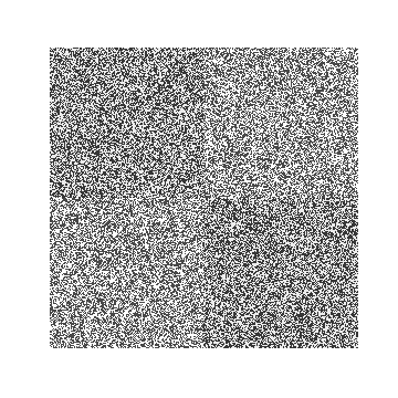
(b) Noisy $A^{\prime}=A+X$

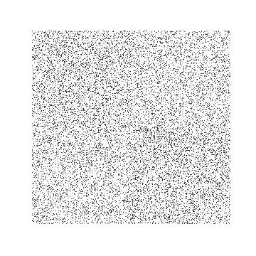
(c) Sampled version of $A^{\prime}$

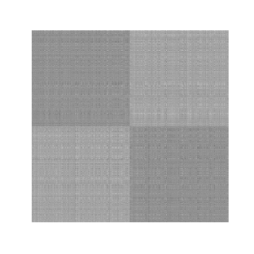
(d) Recovered

Figure 1. Approximate-and-Round run on $\tilde{A}=A^{\prime}+E^{\prime}$ as defined in (17), where $A$ is a $N\times N$ block matrix of $16$’s and $18$’s and $X$ is a $\pm 10$, mean zero, random matrix. Here, $N=20,000$ and the sampling density is $p=0.35$.

The outline of the rest of the paper.

We first collect preparatory tools from linear algebra and probability in Section 4. Then, we prove the deterministic Theorem 6 in Sections 5, 6, and 7. The proof of Theorem 10 from Theorem 6 is given in Section 8. Afterward, we present the proof of the delocalization lemma, Lemma 17, in Sections 9, 10, and 11. Next, we demonstrate in Section 12 that Theorem 15 follows fairly easily from the proof of Lemma 17. To conclude, we discuss in detail (with proofs) our applications in Sections 13 and 14.

4. Preparation

Throughout the paper, we will make repeated use of a few facts from linear algebra and probability. To make the exposition easier, we will collect these facts and some of their consequences here.

4.1. Linear Algebra

Fact 25 (Weyl inequality).

Let $A$ be a symmetric matrix with eigenvalues $\lambda_{1}\geq\lambda_{2}\geq...\geq\lambda_{n}$ and singular values $\sigma_{1}\geq\sigma_{2}\geq...\geq\sigma_{n}$. Define $\tilde{A}=A+H$ for any symmetric matrix $H$. Assume that $\tilde{A}$ has eigenvalues and singular values $\tilde{\lambda}_{i}$ and $\tilde{\sigma}_{i}$, again ordered decreasingly. For all $1\leq i\leq n$,

$$\begin{split}\sigma_{i}-\left\lVert H\right\rVert&\leq\tilde{\sigma}_{i}\leq\sigma_{i}+\left\lVert H\right\rVert,\text{ and }\\ \lambda_{i}-\left\lVert H\right\rVert&\leq\tilde{\lambda}_{i}\leq\lambda_{i}+\left\lVert H\right\rVert.\end{split}$$ (18)

As an immediate consequence, we have the following two results.

1. If $\sigma_{i}\geq 2\left\lVert H\right\rVert$, then $\tilde{\sigma}_{i}\geq\frac{\sigma_{i}}{2}$.

2. If $|\lambda_{i}|>\left\lVert H\right\rVert$, then $\tilde{\lambda}_{i}$ has the same sign as $\lambda_{i}$.

For any symmetric matrix $H$ and index set $\alpha$, let $H^{\alpha}$ be equal be the matrix obtained from $H$ by zeroing out the rows and columns indexed by $\alpha$ (replacing all entries in these rows and columns by zeros). The following fact is well known and easy to prove.

Fact 26.

For any index set $\alpha$, $\left\lVert H^{\alpha}\right\rVert\leq\left\lVert H\right\rVert$.

4.2. Probability

Lemma 27 (Hoeffding’s Inequality, Theorem 2.2.6 in [58]).

Let $X_{1},X_{2},...X_{n}$ be independent zero-mean random variables such that $a_{i}<X_{i}<b_{i}$ with probability $1$. Then,

$$\mathbb{P}\Big{\{}\lvert\sum_{i=1}^{n}X_{i}\rvert>t\Big{\}}\leq 2\exp\Big{(}\frac{-2t^{2}}{\sum_{i=1}^{n}(b_{i}-a_{i})^{2}}\Big{)}.$$ (19)

Corollary 28.

Let $\bf x$ be a random vector whose entries are independent, zero-mean, K-bounded random variables. Then for any fixed unit vector $\mathbf{u}$ and any $C>0$,

$$\mathbb{P}\{|{\bf x}^{T}\mathbf{u}|\geq CK\sqrt{\log n}\}\leq 2\exp(-\frac{C^{2}}{2}\log n)=2n^{-C^{2}/2}.$$

The same bound holds if $\mathbf{u}$ is a random unit vector from which $\mathbf{x}$ is independent.

.

Lemma 29 (Bernstein’s Inequality, Theorem 2.8.4 in [58]).

Let $X_{1},\dots X_{n}$ be independent, $K$ bounded, mean zero, random variables. Then

$$\mathbb{P}\Big{\{}\lvert\sum_{i=1}^{n}a_{i}X_{i}\rvert\geq t\Big{\}}\leq 2\exp\Big{(}-\frac{t^{2}/2}{\sum_{i=1}^{n}\mathbb{E}[X_{i}^{2}]+Kt/3}\Big{)}.$$ (20)

The following is a corollary of a result from [52]; see Appendix A for the proof.

Theorem 30.

Suppose that $E$ is a symmetric random matrix with $K$-bounded, mean zero, independent entries above the diagonal. Suppose that $A$ has rank $r$, and let $1\leq k\leq r$ be an integer. Then, for any $t\geq 0$, the following hold.

$$\begin{split}\mathbb{P}\{\tilde{\sigma}_{k}<\sigma_{k}-t\}&\leq 4\times 9^{k}\exp\Big{(}-\frac{t^{2}}{128K^{2}}\Big{)},\text{ and }\\ \mathbb{P}\Bigg{\{}\tilde{\sigma}_{k}>\sigma_{k}+t\sqrt{r}+2\sqrt{k}\frac{\left\lVert E\right\rVert^{2}}{\tilde{\sigma}_{k}}+k\frac{\left\lVert E\right\rVert^{3}}{\tilde{\sigma}^{2}_{k}}\Bigg{\}}&\leq 4\times 9^{2r}\exp\Big{(}-r\frac{t^{2}}{128K^{2}}\Big{)}.\end{split}$$ (21)

In particular,

$$\mathbb{P}\Big{\{}\lvert\tilde{\sigma}_{k}-\sigma_{k}\rvert>2r\Big{(}t+\frac{\left\lVert E\right\rVert^{2}}{\tilde{\sigma_{k}}}+\frac{\left\lVert E\right\rVert^{3}}{\tilde{\sigma}_{k}^{2}}\Big{)}\Big{\}}\leq 8\times 9^{2r}\exp\Big{(}-\frac{t^{2}}{128K^{2}}\Big{)}.$$

5. Proof of Theorem 6

In this proof, both $A$ and $H$ are deterministic. We will examine the effect of the full perturbation $H$ on entry $u_{il}$ by first considering the auxiliary perturbation $H^{\{l\}}$ (which is obtained from $H$ by leaving out the $l$th row and column). This is an example of the so-called leave-one-out strategy, which has been used by many researchers in recent studies [4, 33, 25, 63, 64]. Next, we need to add the $l$th row and column back and consider the impact of these. This is the more technical part of the proof, which requires a careful analysis.

Let $H_{\{l\}}=H-H^{\{l\}}$. By definition, the entries outside the $l$th row and column of $H_{\{l\}}$ are all zero. We set $A^{\{l\}}:=A+H^{\{l\}}$ and call the singular values and singular vectors of this matrix $\sigma^{\{l\}}_{i}$ and $\mathbf{u}^{\{l\}}_{i}$, respectively. The $l$th entry of $\mathbf{u}^{\{l\}}_{i}$ is $u^{\{l\}}_{il}$.

First, we show that the effect of $H^{\{l\}}$ on $u_{il}$ is extremely small. This is the content of Lemma 31. Once this is established, we view $\tilde{A}$ as a perturbation of $A^{\{l\}}$, $\tilde{A}=A^{\{l\}}+H_{\{l\}}$. The structure of $H_{\{l\}}$ (now viewed as noise) will allow us to deduce a strong $\ell_{2}$ bound for the leading singular vectors of $\tilde{A}$. The key here is that this bound will be so strong that even when we use it to upper bound the entry-wise perturbation, the result still leads to the claim of our theorem. This bound is the content of Lemma 32, which is the most technical part of the proof and requires some novel ideas, going far beyond applying the standard Davis-Kahan bound.

Lemma 31.

Under the conditions of Theorem 6, for any $1\leq l\leq n$,

$$\lvert u^{\{l\}}_{il}-u_{il}\rvert\leq 2r\left\lVert U_{l,\cdot}\right\rVert_{\infty}\Big{[}\kappa_{i}\left\lVert\tilde{\mathbf{u}}_{i}-\mathbf{u}_{i}\right\rVert_{2}+\kappa_{i}\left\lVert\tilde{\mathbf{u}}_{i}-\mathbf{u}^{\{l\}}_{i}\right\rVert_{2}+\epsilon_{1}(i)\Big{]}.$$

Lemma 32.

Under the conditions of Theorem 6, for any $1\leq l\leq n$,

$$\begin{split}\left\lVert\tilde{\mathbf{u}}_{i}-\mathbf{u}^{\{l\}}_{i}\right\rVert_{2}&\leq 68r^{1/2}\Big{[}[\epsilon_{1}(i)+a_{l}\epsilon_{2}(i)]\lvert\tilde{u}_{il}\rvert+\kappa_{i}a_{l}\left\lVert U_{l,\cdot}\right\rVert_{\infty}\epsilon_{2}(i)\Big{]}+32\frac{\lvert\langle\mathbf{u}^{\{l\}}_{i},\mathbf{x}\rangle\rvert}{\sigma_{i}}.\end{split}$$

Proof of Theorem 6 given the lemmas.

By the triangle inequality and the fact that $\ell_{2}$ norm dominates the $\ell_{\infty}$ norm, we have

$$\begin{split}\lvert\tilde{u}_{il}-u_{il}\rvert&\leq\lvert u^{\{l\}}_{il}-u_{il}\rvert+\left\lVert\tilde{\mathbf{u}}_{i}-\mathbf{u}^{\{l\}}_{i}\right\rVert_{2}.\\ \end{split}$$

By Lemma 31, we have

$$\begin{split}\lvert\tilde{u}_{il}-u_{il}\rvert&\leq\lvert u^{\{l\}}_{il}-u_{il}\rvert+\left\lVert\tilde{\mathbf{u}}_{i}-\mathbf{u}^{\{l\}}_{i}\right\rVert_{2}\\ &\leq 2r\left\lVert U_{l,\cdot}\right\rVert_{\infty}(\kappa_{i}\left\lVert\tilde{\mathbf{u}}_{i}-\mathbf{u}_{i}\right\rVert_{2}+\kappa_{i}\left\lVert\tilde{\mathbf{u}}_{i}-\mathbf{u}^{\{l\}}_{i}\right\rVert_{2}+\epsilon_{1}(i))+\left\lVert\tilde{\mathbf{u}}_{i}-\mathbf{u}^{\{l\}}_{i}\right\rVert_{2}\\ &\leq 2r\left\lVert U_{l,\cdot}\right\rVert_{\infty}(\kappa_{i}\left\lVert\tilde{\mathbf{u}}_{i}-\mathbf{u}_{i}\right\rVert_{2}+\epsilon_{1}(i))+4r\left\lVert\tilde{\mathbf{u}}_{i}-\mathbf{u}^{\{l\}}_{i}\right\rVert_{2}.\end{split}$$

Now using Lemma 32 to bound $\left\lVert\tilde{\mathbf{u}}_{i}-\mathbf{u}^{\{l\}}_{i}\right\rVert_{2}$, we obtain, with $C_{0}=4*272r^{3/2}$,

$$\lvert\tilde{u}_{il}-u_{il}\rvert\leq\frac{C_{0}}{4}\Big{[}\kappa_{i}\left\lVert U_{l,\cdot}\right\rVert_{\infty}\left\lVert\tilde{\mathbf{u}}_{i}-\mathbf{u}_{i}\right\rVert_{2}+[\epsilon_{1}(i)+a_{l}\kappa_{i}\epsilon_{2}(i)]\left\lVert U_{l,\cdot}\right\rVert_{\infty}+[\epsilon_{1}(i)+a_{l}\epsilon_{2}(i)]\lvert\tilde{u}_{il}\rvert\Big{]}+128r\frac{\lvert\langle\mathbf{u}^{\{l\}}_{i},\mathbf{x}\rangle\rvert}{\sigma_{i}}.$$

By the triangle inequality, we can bound $\lvert\tilde{u}_{il}\rvert\leq\lvert u_{il}\rvert+\lvert\tilde{u}_{il}-u_{il}\rvert$. This gives, letting $b=\epsilon_{1}(i)+a_{l}\epsilon_{2}(i)$,

$$\lvert\tilde{u}_{il}-u_{il}\rvert\leq\frac{C_{0}}{4}\Big{[}\kappa_{i}\left\lVert U_{l,\cdot}\right\rVert_{\infty}\left\lVert\tilde{\mathbf{u}}_{i}-\mathbf{u}_{i}\right\rVert_{2}+b\left\lVert U_{l,\cdot}\right\rVert_{\infty}+b(\lvert u_{il}\rvert+\lvert\tilde{u}_{il}-u_{il}\rvert)\Big{]}+128r\frac{\lvert\langle\mathbf{u}^{\{l\}}_{i},\mathbf{x}\rangle\rvert}{\sigma_{i}}.$$

Then, the coefficient in front of $\lvert\tilde{u}_{il}-u_{il}\rvert$ on the RHS is $\frac{C_{0}b}{4}$. Recall that $\epsilon_{1}(i)=\frac{\left\lVert E\right\rVert}{\sigma_{i}}$ and $\epsilon_{2}(i)=\frac{1}{\delta_{i}}$. Therefore, because $\sigma_{i}\geq C_{0}\left\lVert E\right\rVert$ and $\delta_{i}\geq C_{0}a_{l}$, it must be the case that $b<\frac{2}{C_{0}}$. Then we can move all the terms with $\lvert\tilde{u}_{il}-u_{il}\rvert$ to the left with coefficient at most $1/2$. This gives

$$\frac{1}{2}|u_{ij}-\tilde{u}_{ij}|\leq\frac{C_{0}}{4}\Big{[}\kappa_{i}\left\lVert U_{l,\cdot}\right\rVert_{\infty}\left\lVert\tilde{\mathbf{u}}_{i}-\mathbf{u}_{i}\right\rVert_{2}+b\left\lVert U_{l,\cdot}\right\rVert_{\infty}+b\lvert u_{il}\rvert\Big{]}+128r\frac{\lvert\langle\mathbf{u}^{\{l\}}_{i},\mathbf{x}\rangle\rvert}{\sigma_{i}}.$$ (22)

Bounding the term $\lvert u_{il}\rvert$ on the RHS by $\left\lVert U_{l,\cdot}\right\rVert_{\infty}$, we obtain

$$\frac{1}{2}\lvert\tilde{u}_{il}-u_{il}\rvert\leq\frac{C_{0}\left\lVert U_{l,\cdot}\right\rVert_{\infty}}{4}\Big{[}\kappa_{i}\left\lVert\tilde{\mathbf{u}}_{i}-\mathbf{u}_{i}\right\rVert_{2}+2b\Big{]}+128r\frac{\lvert\langle\mathbf{u}^{\{l\}}_{i},\mathbf{x}\rangle\rvert}{\sigma_{i}}.$$

Multiplying both sides by $2$, we obtain the desired inequality (with room to spare).

∎

In the next two sections, we establish Lemmas 31 and 32, respectively.

6. Proof of Lemma 31

Recall that for a matrix $M$, $M_{l,\cdot}$ denotes the $l$th row of $M$, viewed as a vector. The key point of the leave-one-out analysis is that by definition, $A^{\{l\}}_{l,\cdot}=A_{l,\cdot}$. Furthermore, as $\mathbf{u}^{\{l\}}_{i}$ is a singular vector of $A^{\{l\}}$, $A^{\{l\}}\mathbf{u}^{\{l\}}_{i}$ is either $\sigma^{\{l\}}_{i}\mathbf{u}^{\{l\}}_{i}$ or $-\sigma^{\{l\}}_{i}\mathbf{u}^{\{l\}}_{i}$ and we will use the shorthand $A^{\{l\}}\mathbf{u}^{\{l\}}_{i}=\pm\sigma^{\{l\}}_{i}\mathbf{u}^{\{l\}}_{i}$. In all estimates where this shorthand appears, the sign does not matter. Since $A^{\{l\}}\mathbf{u}^{\{l\}}_{i}=\pm\sigma_{i}^{\{l\}}\mathbf{u}^{\{l\}}_{i}$,

$$u^{\{l\}}_{il}=\frac{\langle A^{\{l\}}_{l,\cdot},\mathbf{u}^{\{l\}}_{i}\rangle}{\pm\sigma_{i}^{\{l\}}}=\frac{\langle A_{l,\cdot},\mathbf{u}^{\{l\}}_{i}\rangle}{\pm\sigma_{i}^{\{l\}}}.$$

By the spectral decomposition of $A$, the RHS can be written as

$$\frac{\langle A_{l,\cdot},\mathbf{u}^{\{l\}}_{i}\rangle}{\pm\sigma_{i}^{\{l\}}}=\frac{1}{\pm\sigma_{i}^{\{l\}}}\Big{[}\pm\sigma_{1}u_{1l}\mathbf{u}_{1}^{T}\pm\sigma_{2}u_{2l}\mathbf{u}^{T}_{2}+\dots\pm\sigma_{r}u_{rl}\mathbf{u}^{T}_{r}\Big{]}\mathbf{u}^{\{l\}}_{i},$$

which implies, via the triangle inequality, that

$$\lvert u^{\{l\}}_{il}-u_{il}\rvert\leq\Bigg{\lvert}\frac{\sigma_{i}}{\sigma_{i}^{\{l\}}}u_{il}\mathbf{u}_{i}^{T}\mathbf{u}^{\{l\}}_{i}-u_{il}\Bigg{\rvert}+\Bigg{\lvert}\frac{1}{\sigma_{i}^{\{l\}}}\sum_{j\neq i}^{r}\pm\sigma_{j}u_{jl}\mathbf{u}_{j}^{T}\mathbf{u}^{\{l\}}_{i}\Bigg{\rvert}.$$

In the first term on the RHS, we have eliminated the signs in front of $\sigma_{i}$ and $\sigma^{\{l\}}_{i}$. This is because their signs correspond to the signs of the corresponding eigenvalues of $A$ and $A^{\{l\}}$ respectively. It must be the case that these eigenvalues have the same sign by Fact 25. Studying the second term on the RHS, write $\mathbf{u}^{\{l\}}_{i}=\mathbf{u}_{i}+(\mathbf{u}^{\{l\}}_{i}-\mathbf{u}_{i})$. By the orthogonality of $\mathbf{u}_{i}$ with $\mathbf{u}_{j}$ for $j\neq i$, it follows that

$$\lvert u^{\{l\}}_{il}-u_{il}\rvert\leq\lvert\frac{\sigma_{i}}{\sigma^{\{l\}}_{i}}u_{il}\mathbf{u}_{i}^{T}\mathbf{u}^{\{l\}}_{i}-u_{il}\rvert+\frac{2}{\sigma_{i}}\sum_{j\neq i}^{r}\sigma_{j}\lvert u_{jl}\rvert\left\lVert\mathbf{u}^{\{l\}}_{i}-\mathbf{u}_{i}\right\rVert_{2}.$$ (23)

To bound first term on the right hand side of (23), write

$$\begin{split}\frac{\sigma_{i}}{\sigma_{i}^{\{l\}}}u_{il}\mathbf{u}_{i}^{T}\mathbf{u}^{\{l\}}_{i}-u_{il}&=u_{il}\Bigg{(}\frac{\sigma_{i}-\sigma_{i}^{\{l\}}}{\sigma_{i}^{\{l\}}}\Bigg{)}\mathbf{u}_{i}^{T}\mathbf{u}^{\{l\}}_{i}+u_{il}\mathbf{u}_{i}^{T}(\mathbf{u}^{\{l\}}_{i}-\mathbf{u}_{i}).\end{split}$$ (24)

Since $\sigma_{i}^{\{l\}}>\sigma_{i}/2$ by Facts 25 and 26, the triangle inequality gives

$$\begin{split}\lvert\frac{\sigma_{i}}{\sigma_{i}^{\{l\}}}u_{il}\mathbf{u}_{i}^{T}\mathbf{u}^{\{l\}}_{i}-u_{il}\rvert&\leq\lvert u_{il}\rvert\frac{\lvert\sigma_{i}-\sigma_{i}^{\{l\}}\rvert}{\sigma_{i}^{\{l\}}}\left\lVert\mathbf{u}_{i}\right\rVert_{2}\left\lVert\mathbf{u}^{\{l\}}_{i}\right\rVert_{2}+\lvert u_{il}\rvert\left\lVert\mathbf{u}_{i}\right\rVert_{2}\left\lVert\mathbf{u}^{\{l\}}_{i}-\mathbf{u}_{i}\right\rVert_{2}\\ &\leq 2\lvert u_{il}\rvert\frac{\left\lVert H\right\rVert}{\sigma_{i}}+\lvert u_{il}\rvert\left\lVert\mathbf{u}^{\{l\}}_{i}-\mathbf{u}_{i}\right\rVert_{2}\\ &\leq 2\epsilon_{1}(i)\left\lVert U_{l,\cdot}\right\rVert_{\infty}+\left\lVert\mathbf{u}^{\{l\}}_{i}-\mathbf{u}_{i}\right\rVert_{2}\left\lVert U_{l,\cdot}\right\rVert_{\infty}.\end{split}$$ (25)

The second line uses Fact 25 to bound $\lvert\sigma_{i}-\sigma_{i}^{\{l\}}\rvert\leq\left\lVert H^{\{l\}}\right\rVert$, and Fact 26 to get $\left\lVert H^{\{l\}}\right\rVert\leq\left\lVert H\right\rVert$. To bound the second term on the RHS of (23), bound $\lvert u_{il}\rvert\leq\left\lVert U_{l,\cdot}\right\rVert_{\infty}$ to obtain

$$\frac{2}{\sigma_{i}}\sum_{j\neq i}^{r}\sigma_{j}\lvert u_{jl}\rvert\left\lVert\mathbf{u}^{\{l\}}_{i}-\mathbf{u}_{i}\right\rVert_{2}\leq 2\left\lVert U_{l,\cdot}\right\rVert_{\infty}\frac{\left\lVert\mathbf{u}^{\{l\}}_{i}-\mathbf{u}_{i}\right\rVert_{2}\sigma_{1}(r-1)}{\sigma_{i}}.$$

We can bound this last term by $2\kappa_{i}\left\lVert U_{l,\cdot}\right\rVert_{\infty}\left\lVert\mathbf{u}^{\{l\}}_{i}-\mathbf{u}_{i}\right\rVert_{2}(r-1)$ to conclude that

$$\begin{split}\lvert u^{\{l\}}_{il}-u_{il}\rvert&\leq 2\epsilon_{1}(i)\left\lVert U_{l,\cdot}\right\rVert_{\infty}+\left\lVert\mathbf{u}^{\{l\}}_{i}-\mathbf{u}_{i}\right\rVert_{2}\left\lVert U_{l,\cdot}\right\rVert_{\infty}+2\kappa_{i}\left\lVert U_{l,\cdot}\right\rVert_{\infty}\left\lVert\mathbf{u}^{\{l\}}_{i}-\mathbf{u}_{i}\right\rVert_{2}(r-1)\\ &\leq 2r\kappa_{i}\left\lVert U_{l,\cdot}\right\rVert_{\infty}\left\lVert\mathbf{u}^{\{l\}}_{i}-\mathbf{u}_{i}\right\rVert_{2}+2\epsilon_{1}(i)\left\lVert U_{l,\cdot}\right\rVert_{\infty}\\ &\leq 2r\Big{[}\kappa_{i}\left\lVert U_{l,\cdot}\right\rVert_{\infty}\left\lVert\tilde{\mathbf{u}}_{i}-\mathbf{u}_{i}\right\rVert_{2}+\kappa_{i}\left\lVert U_{l,\cdot}\right\rVert_{\infty}\left\lVert\tilde{\mathbf{u}}_{i}-\mathbf{u}^{\{l\}}_{i}\right\rVert_{2}+\epsilon_{1}(i)\left\lVert U_{l,\cdot}\right\rVert_{\infty}\Big{]}.\end{split}$$ (26)

where the last step uses the triangle inequality. This concludes the proof of Lemma 31.

7. Proof of Lemma 32

In this section, we will view $\tilde{A}$ as a perturbation of $A^{\{l\}}$ with the perturbing matrix $H_{\{l\}}$. The main idea is that $H_{\{l\}}$ is only supported on one row and one column. By leveraging this and $\left\lVert U_{l,\cdot}\right\rVert_{\infty}$, we can obtain a strong bound for $\left\lVert\tilde{\mathbf{u}}_{i}-\mathbf{u}^{\{l\}}_{i}\right\rVert_{2}$. We begin with the following decomposition which will prove useful throughout:

$$H_{\{l\}}=\mathbf{x}\mathbf{e}_{l}^{T}+\mathbf{e}_{l}\mathbf{x}^{T}.$$ (27)

Recall that $\mathbf{x}$ is the $l$th row of $H$, but with the $l$th entry set to $H_{ll}/2$, as $H_{\{l\}}$ is $H-H^{\{l\}}$. Define $p=\min\{j:\sigma_{j+1}<\sigma_{i}/4\}$. Let $P^{\{l\}}$ be the orthogonal projection to the orthogonal complement of the columns of $U^{\{l\}}_{p}$, and let $V^{\{l\}}_{p}$ be the $n\times(p-1)$ matrix whose columns are $\mathbf{u}^{\{l\}}_{1},\dots,\mathbf{u}^{\{l\}}_{i-1},\mathbf{u}^{\{l\}}_{i+1},\dots,\mathbf{u}^{\{l\}}_{p}$. Expanding $\tilde{\mathbf{u}}_{i}$ in the coordinates of the orthonormal basis $\{\mathbf{u}^{\{l\}}_{k}\}_{1\leq k\leq n}$,

$$\tilde{\bf u}_{i}=\sum_{k=1}^{p}\alpha_{k}{\bf u}_{k}^{\{l\}}+P^{\{l\}}\tilde{\mathbf{u}}_{i}.$$

It follows that

$$\begin{split}\left\lVert\tilde{\mathbf{u}}_{i}-\mathbf{u}^{\{l\}}_{i}\right\rVert^{2}_{2}&=\langle\tilde{\mathbf{u}}_{i},\tilde{\mathbf{u}}_{i}\rangle+\langle\mathbf{u}^{\{l\}}_{i},\mathbf{u}^{\{l\}}_{i}\rangle-2\langle\tilde{\mathbf{u}}_{i},\mathbf{u}^{\{l\}}_{i}\rangle\\ &=2(1-\alpha_{i}^{2})\\ &=2\sum_{k\neq i}^{n}\alpha_{k}^{2}\\ &=2\sum_{k\neq i}^{p}\alpha_{k}^{2}+2\left\lVert P^{\{l\}}\tilde{\mathbf{u}}_{i}\right\rVert_{2}^{2}\\ &=2\left\lVert V^{\{l\}T}_{p}\tilde{\mathbf{u}}_{i}\right\rVert_{2}^{2}+2\left\lVert P^{\{l\}}\tilde{\mathbf{u}}_{i}\right\rVert_{2}^{2}.\end{split}$$ (28)

Therefore,

$$\left\lVert\tilde{\mathbf{u}}_{i}-\mathbf{u}^{\{l\}}_{i}\right\rVert_{2}\leq\sqrt{2}\Big{[}\left\lVert V^{\{l\}T}_{p}\tilde{\mathbf{u}}_{i}\right\rVert_{2}+\left\lVert P^{\{l\}}\tilde{\mathbf{u}}_{i}\right\rVert_{2}\Big{]}.$$ (29)

Proving Lemma 32 reduces to bounding the two terms on the RHS. It is possible that the first term in the fourth line of (28) is a sum over an empty set (say $i=1,p=1$). In this case, $\left\lVert\tilde{\mathbf{u}}_{i}-\mathbf{u}^{\{l\}}_{i}\right\rVert_{2}\leq\sqrt{2}\left\lVert P^{\{l\}}\tilde{\mathbf{u}}_{i}\right\rVert_{2}.$

Lemma 33 ($\left\lVert P^{\{l\}}\tilde{\mathbf{u}}_{i}\right\rVert_{2}$ Bound).

$$\left\lVert P^{\{l\}}\tilde{\mathbf{u}}_{i}\right\rVert_{2}\leq 24\epsilon_{1}(i)(\lvert\tilde{u}_{il}\rvert+\left\lVert\tilde{\mathbf{u}}_{i}-\mathbf{u}^{\{l\}}_{i}\right\rVert_{2})+8\frac{\lvert\langle\mathbf{x},\mathbf{u}^{\{l\}}_{i}\rangle\rvert}{\sigma_{i}}.$$ (30)

As we previously observed, there is no contribution from $\left\lVert V^{\{l\}T}_{p}\tilde{\mathbf{u}}_{i}\right\rVert_{2}$ when the aforementioned sum is empty. So we assume without loss of generality that it is not. We first establish that it is sufficient to bound the quantity $\left\lVert U^{\{l\}T}_{p}H_{\{l\}}\tilde{\mathbf{u}}_{i}\right\rVert_{2}$ by using the perturbation technique of [52]. This is the content of the following proposition, which is where we use the gap stability condition.

Proposition 34.

$$\left\lVert V^{\{l\}T}_{p}\tilde{\mathbf{u}}_{i}\right\rVert_{2}\leq 2\epsilon_{2}(i)\left\lVert U^{\{l\}T}_{p}H_{\{l\}}\tilde{\mathbf{u}}_{i}\right\rVert_{2}.$$ (31)

Having established this, when we go to bound $\left\lVert U^{\{l\}T}_{p}H_{\{l\}}\tilde{\mathbf{u}}_{i}\right\rVert_{2}$, the structure of $H_{\{l\}}$ will bring the $l$th row of $U^{\{l\}}_{p}$ into play. It is important that this row not be too large in norm.

Proposition 35 (The $l$th row of $U^{\{l\}}_{p}$ is small).

Let $\mathbf{r}^{\{l\}}$ denote the $l$th row of $U^{\{l\}}_{p}$ viewed as a column vector. Then

$$\begin{split}\left\lVert\mathbf{r}^{\{l\}}\right\rVert_{2}\leq 8r^{1/2}\kappa_{i}\left\lVert U_{l,\cdot}\right\rVert_{\infty}.\end{split}$$ (32)

The two propositions can be shown to give us a bound for $\left\lVert V^{\{l\}T}_{p}\tilde{\mathbf{u}}_{i}\right\rVert_{2}$.

Lemma 36.

$$\left\lVert V^{\{l\}T}_{p}\tilde{\mathbf{u}}_{i}\right\rVert_{2}\leq 16r^{1/2}\epsilon_{2}(i)\Big{[}a_{l}(\lvert\tilde{u}_{il}\rvert+\kappa_{i}\left\lVert U_{l,\cdot}\right\rVert_{\infty})+\kappa_{i}\left\lVert H\right\rVert\left\lVert U_{l,\cdot}\right\rVert_{\infty}\left\lVert\tilde{\mathbf{u}}_{i}-\mathbf{u}^{\{l\}}_{i}\right\rVert_{2}\Big{]}.$$ (33)

We are now ready to prove Lemma 32.

Proof of Lemma 32 given Lemmas 33 and 36.

Lemmas 33 and 36 can be used to bound the RHS of (29). In particular, temporarily setting $\beta:=\left\lVert\tilde{\mathbf{u}}_{i}-\mathbf{u}^{\{l\}}_{i}\right\rVert_{2}$ for brevity,

$$\begin{split}\beta&\leq\sqrt{2}\Big{[}\left\lVert V^{\{l\}T}_{p}\tilde{\mathbf{u}}_{i}\right\rVert_{2}+\left\lVert P^{\{l\}}\tilde{\mathbf{u}}_{i}\right\rVert_{2}\Big{]}\\ &\leq 34r^{1/2}\Big{[}\epsilon_{1}(i)\lvert\tilde{u}_{il}\rvert+a_{l}\epsilon_{2}(i)(\lvert\tilde{u}_{il}\rvert+\kappa_{i}\left\lVert U_{l,\cdot}\right\rVert_{\infty})+[\epsilon_{1}(i)+\kappa_{i}\left\lVert H\right\rVert\left\lVert U_{l,\cdot}\right\rVert_{\infty}\epsilon_{2}(i)]\beta\Big{]}+16\frac{\lvert\langle\mathbf{x},\mathbf{u}^{\{l\}}_{i}\rangle\rvert}{\sigma_{i}}.\end{split}$$ (34)

The main observation is that $\beta$ appears on both the LHS and RHS of the inequality. The coefficient of $\beta$ in the RHS is $34r^{1/2}[\epsilon_{1}(i)+\kappa_{i}\left\lVert H\right\rVert\left\lVert U_{l,\cdot}\right\rVert_{\infty}\epsilon_{2}(i)]$. By the definition of $\epsilon_{1}(i)$ and $\epsilon_{2}(i)$ (see the discussion preceding Theorem 6), this equals $34r^{1/2}(\frac{\left\lVert H\right\rVert}{\sigma_{i}}+\kappa_{i}\left\lVert H\right\rVert\left\lVert U_{l,\cdot}\right\rVert)$. By the definition of $C_{0}$, and the assumption that $\sigma_{i}>C_{0}\left\lVert E\right\rVert$ and $\delta_{i}>C_{0}\kappa_{i}\left\lVert H\right\rVert\left\lVert U\right\rVert_{\infty}$, we have the following estimate.

$$\begin{split}\beta&\leq 34r^{1/2}\Big{[}\epsilon_{1}(i)\lvert\tilde{u}_{il}\rvert+a_{l}\epsilon_{2}(i)(\lvert\tilde{u}_{il}\rvert+\kappa_{i}\left\lVert U_{l,\cdot}\right\rVert_{\infty})\Big{]}+\frac{1}{2}\beta+16\frac{\lvert\langle\mathbf{x},\mathbf{u}^{\{l\}}_{i}\rangle\rvert}{\sigma_{i}}.\end{split}$$ (35)

Therefore, moving the terms involving $\beta$ to the left and multiplying both sides by $2$ gives

$$\begin{split}\left\lVert\tilde{\mathbf{u}}_{i}-\mathbf{u}^{\{l\}}_{i}\right\rVert_{2}&\leq 68r^{1/2}\Big{[}[\epsilon_{1}(i)+a_{l}\epsilon_{2}(i)]\lvert\tilde{u}_{il}\rvert+\kappa_{i}a_{l}\left\lVert U_{l,\cdot}\right\rVert_{\infty}\epsilon_{2}(i)\Big{]}+32\frac{\lvert\langle\mathbf{x},\mathbf{u}^{\{l\}}_{i}\rangle\rvert}{\sigma_{i}}.\end{split}$$

∎

Proof of Lemma 33.

Since $\tilde{A}-A^{\{l\}}=H_{\{l\}}$, it follows that

$$(P^{\{l\}}\tilde{\mathbf{u}}_{i})^{T}\tilde{A}\tilde{\mathbf{u}}_{i}-(P^{\{l\}}\tilde{\mathbf{u}}_{i})^{T}A^{\{l\}}\tilde{\mathbf{u}}_{i}=(P^{\{l\}}\tilde{\mathbf{u}}_{i})^{T}H_{\{l\}}\tilde{\mathbf{u}}_{i}.$$ (36)

By the definition of $P^{\{l\}}$, we have

$$\lvert(P^{\{l\}}\tilde{\mathbf{u}}_{i})^{T}A^{\{l\}}\tilde{\mathbf{u}}_{i}\rvert=\lvert\langle P^{\{l\}}\tilde{\mathbf{u}}_{i},A^{\{l\}}\tilde{\mathbf{u}}_{i}\rangle\rvert=\lvert\langle\tilde{\mathbf{u}}_{i},P^{\{l\}}A^{\{l\}}\tilde{\mathbf{u}}_{i}\rangle\rvert\leq\sigma_{p+1}^{\{l\}}\left\lVert P^{\{l\}}\mathbf{u}_{i}\right\rVert_{2}^{2}.$$ (37)

By Fact 25, $\sigma_{p+1}^{\{l\}}\leq\sigma_{p+1}+\|H^{\{l\}}\|.$ Furthermore, by Fact 26, $\|H^{\{l\}}\|\leq\|H\|$, so we have $\sigma^{\{l\}}_{p+1}\leq\sigma_{p+1}+\left\lVert H\right\rVert$. Because $\tilde{\mathbf{u}}_{i}$ is a singular vector of $\tilde{A}$, we have

$$(P^{\{l\}}\tilde{\mathbf{u}}_{i})^{T}\tilde{A}\tilde{\mathbf{u}}_{i}=\pm\tilde{\sigma}_{i}\left\lVert P^{\{l\}}\tilde{\mathbf{u}}_{i}\right\rVert_{2}^{2}.$$

It thus follows that

$$\tilde{\sigma}_{i}\left\lVert P^{\{l\}}\tilde{\mathbf{u}}_{i}\right\rVert_{2}^{2}-(\sigma_{p+1}+\left\lVert H\right\rVert)\left\lVert P^{\{l\}}\tilde{\mathbf{u}}_{i}\right\rVert_{2}^{2}\leq|(P^{\{l\}}\tilde{\mathbf{u}}_{i})^{T}H_{\{l\}}\tilde{\mathbf{u}}_{i}|.$$ (38)

Applying Cauchy-Schwarz on the RHS, we obtain

$$\tilde{\sigma}_{i}\left\lVert P^{\{l\}}\tilde{\mathbf{u}}_{i}\right\rVert_{2}^{2}-(\sigma_{p+1}+\left\lVert H\right\rVert)\left\lVert P^{\{l\}}\tilde{\mathbf{u}}_{i}\right\rVert_{2}^{2}\leq\left\lVert P^{\{l\}}\tilde{\mathbf{u}}_{i}\right\rVert_{2}\left\lVert H_{\{l\}}\tilde{\mathbf{u}}_{i}\right\rVert_{2}.$$ (39)

By Fact 25, $\tilde{\sigma}_{i}(A)>\frac{\sigma_{i}}{2}$. By definition of $p$, $\frac{\sigma_{i}}{2}-\sigma_{p+1}>\frac{1}{4}\sigma_{i}$. So dividing by $\left\lVert P^{\{l\}}\tilde{\mathbf{u}}_{i}\right\rVert_{2}$ gives

$$\left\lVert P^{\{l\}}\tilde{\mathbf{u}}_{i}\right\rVert_{2}\leq\frac{\left\lVert H_{\{l\}}\tilde{\mathbf{u}}_{i}\right\rVert_{2}}{0.25\sigma_{i}-\left\lVert H\right\rVert}\leq\frac{\left\lVert H_{\{l\}}\mathbf{u}^{\{l\}}_{i}\right\rVert_{2}+\left\lVert H_{\{l\}}\right\rVert\left\lVert\tilde{\mathbf{u}}_{i}-\mathbf{u}^{\{l\}}_{i}\right\rVert_{2}}{0.25\sigma_{i}-\left\lVert H\right\rVert}\leq 8\frac{\left\lVert H_{\{l\}}\mathbf{u}^{\{l\}}_{i}\right\rVert_{2}+2\left\lVert H\right\rVert\left\lVert\tilde{\mathbf{u}}_{i}-\mathbf{u}^{\{l\}}_{i}\right\rVert_{2}}{\sigma_{i}}.$$ (40)

We used the triangle inequality in the numerator. It is apparent that $\mathbf{x}$ has $\ell_{2}$ norm at most that of the $l$th row of $H$. This gave $\left\lVert H_{\{l\}}\right\rVert=\left\lVert\mathbf{x}\mathbf{e}_{l}^{T}+\mathbf{e}_{l}\mathbf{x}^{T}\right\rVert\leq 2\left\lVert\mathbf{x}\right\rVert\leq 2\left\lVert H\right\rVert$. We also lower bounded $0.25\sigma_{i}-\left\lVert H\right\rVert\geq\sigma_{i}/8$ because $\sigma_{i}>C_{0}\left\lVert H\right\rVert$. To estimate the term $\left\lVert H_{\{l\}}\mathbf{u}^{\{l\}}_{i}\right\rVert_{2}$, write using (27),

$$H_{\{l\}}\mathbf{u}^{\{l\}}_{i}=\langle\mathbf{x},\mathbf{u}^{\{l\}}_{i}\rangle\mathbf{e}_{l}+u^{\{l\}}_{il}\mathbf{x}.$$ (41)

Here $\mathbf{e}_{l}$ is the $l$th standard basis vector. We obtain

$$\begin{split}\left\lVert H_{\{l\}}\mathbf{u}^{\{l\}}_{i}\right\rVert_{2}&\leq\lvert\langle\mathbf{x},\mathbf{u}^{\{l\}}_{i}\rangle\rvert+\left\lVert\mathbf{x}\right\rVert_{2}\lvert u^{\{l\}}_{il}\rvert\\ &\leq\lvert\langle\mathbf{x},\mathbf{u}^{\{l\}}_{i}\rangle\rvert+\left\lVert H\right\rVert(\lvert\tilde{u}_{il}\rvert+\lvert\tilde{u}_{il}-u^{\{l\}}_{il}\rvert).\\ \end{split}$$ (42)

So we conclude that

$$\left\lVert P^{\{l\}}\tilde{\mathbf{u}}_{i}\right\rVert_{2}\leq\frac{8\lvert\langle\mathbf{x},\mathbf{u}^{\{l\}}_{i}\rangle\rvert+24\left\lVert H\right\rVert(\lvert\tilde{u}_{il}\rvert+\left\lVert\mathbf{u}^{\{l\}}_{i}-\tilde{\mathbf{u}}_{i}\right\rVert_{2})}{\sigma_{i}},$$ (43)

proving the lemma. ∎

Proof of Proposition 34.

By the relation $\tilde{A}-A^{\{l\}}=H_{\{l\}}$, we have

$$V^{\{l\}T}_{p}\tilde{A}\tilde{\mathbf{u}}_{i}-V^{\{l\}T}_{p}A^{\{l\}}\tilde{\mathbf{u}}_{i}=V^{\{l\}T}_{p}H_{\{l\}}\tilde{\mathbf{u}}_{i}.$$ (44)

First, we observe that because $\tilde{\mathbf{u}}_{i}$ is a singular vector of $\tilde{A}$, the first term on the LHS of (44) is $\pm\tilde{\sigma}_{i}V^{\{l\}T}_{p}\tilde{\mathbf{u}}_{i}$. Since the columns of $V^{\{l\}}_{p}$ are singular vectors of $A^{\{l\}}$, the second term on the left hand side of (44) is $D^{\{l\}}V^{\{l\}T}_{p}\tilde{\mathbf{u}}_{i}$. $D^{\{l\}}$ is the $(p-1)\times(p-1)$ diagonal matrix with entries $\pm\sigma_{1}^{\{l\}},..\pm\sigma_{i-1}^{\{l\}},\pm\sigma_{i+1}^{\{l\}}...\pm\sigma_{p}^{\{l\}}$. Then, we have

$$\left\lVert U^{\{l\}T}_{p}H_{\{l\}}\tilde{\mathbf{u}}_{i}\right\rVert_{2}\geq\left\lVert V^{\{l\}T}_{p}H_{\{l\}}\tilde{\mathbf{u}}_{i}\right\rVert_{2}=\left\lVert(\pm\tilde{\sigma}_{i}I-D^{\{l\}})V^{\{l\}T}_{p}\tilde{\mathbf{u}}_{i}\right\rVert_{2}\geq\frac{\delta_{i}}{2}\left\lVert V^{\{l\}T}_{p}\tilde{\mathbf{u}}_{i}\right\rVert_{2}.$$ (45)

The first inequality uses that $V^{\{l\}T}_{p}H_{\{l\}}\tilde{\mathbf{u}}_{i}$ is a sub-vector of $U^{\{l\}T}_{p}H_{\{l\}}\tilde{\mathbf{u}}_{i}$. The equality uses (44), and the last inequality uses that the smallest singular value of the diagonal matrix $\pm\tilde{\sigma}_{i}I-D^{\{l\}}$ is at least $\delta_{i}/2$ by the assumption of Theorem 6.

∎

Proof of Proposition 35.

Since the columns of $U^{\{l\}}_{p}$ are singular vectors, if $\Sigma^{\{l\}}_{p}$ is a diagonal matrix with entries $\pm\sigma_{1}^{\{l\}},...\pm\sigma_{p}^{\{l\}}$, we have by definition of $\mathbf{r}^{\{l\}}$,

$$\begin{split}\left\lVert\mathbf{r}^{\{l\}}\right\rVert_{2}&=\left\lVert\mathbf{e}_{l}^{T}U^{\{l\}}_{p}\right\rVert_{2}=\left\lVert\mathbf{e}_{l}^{T}A^{\{l\}}U^{\{l\}}_{p}\Sigma^{\{l\}-1}_{p}\right\rVert_{2}.\\ \end{split}$$ (46)

Because $A^{\{l\}}$ and $A$ have the same $l$th row,

$$\left\lVert\mathbf{r}^{\{l\}}\right\rVert_{2}=\left\lVert\mathbf{e}_{l}^{T}AU^{\{l\}}_{p}\Sigma^{\{l\}-1}_{p}\right\rVert_{2}.$$ (47)

By the spectral decomposition of $A$, if $\Sigma$ is the diagonal matrix whose entries are the eigenvalues of $A$, then the the RHS is $\left\lVert\mathbf{e}_{l}^{T}U\Sigma U^{T}U^{\{l\}}_{p}\Sigma^{\{l\}-1}_{p}\right\rVert_{2}=\left\lVert U_{l,\cdot}\Sigma U^{T}U^{\{l\}}_{p}\Sigma^{\{l\}-1}_{p}\right\rVert_{2}$. By the triangle inequality,

$$\left\lVert\mathbf{r}^{\{l\}}\right\rVert_{2}\leq\left\lVert U_{l,\cdot}\right\rVert_{2}\left\lVert\Sigma\right\rVert\left\lVert U^{T}U^{\{l\}}_{p}\right\rVert\left\lVert\Sigma^{\{l\}-1}_{p}\right\rVert_{2}.$$ (48)

Because $\sigma_{1}>C_{0}\left\lVert E\right\rVert$ and the definition of $p$, $\Sigma^{\{l\}-1}_{p}$ has norm at most $\sigma^{\{l\}}_{p}\leq\sigma_{p}/2$ by Facts 25 and 26. It is clear that $\left\lVert\Sigma\right\rVert=\sigma_{1}$ and $\left\lVert U^{T}U^{\{l\}}_{p}\right\rVert\leq 1$. Therefore, since $\left\lVert U_{l,\cdot}\right\rVert_{2}\leq\sqrt{r}\left\lVert U_{l,\cdot}\right\rVert_{\infty}$,

$$\left\lVert\mathbf{r}^{\{l\}}\right\rVert_{2}\leq 2r^{1/2}\Big{(}\frac{\sigma_{1}}{\sigma_{p}}\Big{)}\left\lVert U_{l,\cdot}\right\rVert_{\infty}\leq 8\kappa_{i}r^{1/2}\left\lVert U_{l,\cdot}\right\rVert_{\infty},$$ (49)

where the last inequality uses the definition of $p$.

∎

Proof of Lemma 36.

By Proposition 34, it suffices to upper bound $\left\lVert U^{\{l\}T}_{p}H_{\{l\}}\tilde{\mathbf{u}}_{i}\right\rVert_{2}$. Using the decomposition for $H_{\{l\}}$ (27), we can write

$$U^{\{l\}T}_{p}H_{\{l\}}\tilde{\mathbf{u}}_{i}=(H_{\{l\}}U^{\{l\}}_{p})^{T}\tilde{\mathbf{u}}_{i}=(X+Y)\tilde{\mathbf{u}}_{i}.$$

Thus, we must bound $\left\lVert X\tilde{\mathbf{u}}_{i}\right\rVert_{2}+\left\lVert Y\tilde{\mathbf{u}}_{i}\right\rVert_{2}$, where $X=U^{\{l\}T}_{p}\mathbf{x}\mathbf{e}_{l}^{T}$ and $Y=U^{\{l\}T}_{p}\mathbf{e}_{l}\mathbf{x}^{T}$. Therefore,

$$\left\lVert X\tilde{\mathbf{u}}_{i}\right\rVert_{2}\leq\lvert\tilde{u}_{il}\rvert\left\lVert U_{p}^{\{l\}T}\mathbf{x}\right\rVert_{2}=\lvert\tilde{u}_{il}\rvert a_{l}.$$ (50)

On the other hand, for $\left\lVert Y\tilde{\mathbf{u}}_{i}\right\rVert_{2}$, the triangle inequality gives

$$\left\lVert Y\tilde{\mathbf{u}}_{i}\right\rVert_{2}\leq\left\lVert Y\mathbf{u}^{\{l\}}_{i}\right\rVert_{2}+\left\lVert Y\right\rVert\left\lVert\tilde{\mathbf{u}}_{i}-\mathbf{u}^{\{l\}}_{i}\right\rVert_{2}.$$ (51)

By definition of $Y$, we can write $Y\mathbf{u}^{\{l\}}_{i}=\langle\mathbf{u}^{\{l\}}_{i},\mathbf{x}\rangle U^{\{l\}T}_{p}\mathbf{e}_{l}=\langle\mathbf{u}^{\{l\}}_{i},\mathbf{x}\rangle\mathbf{r}^{\{l\}}$. As before, $\mathbf{e}_{l}$ is the $l$th standard basis vector. Invoking Proposition 35, it follows immediately that

$$\left\lVert Y\mathbf{u}^{\{l\}}_{i}\right\rVert_{2}\leq\lvert\langle\mathbf{u}^{\{l\}}_{i},\mathbf{x}\rangle\rvert\left\lVert\mathbf{r}^{\{l\}}\right\rVert_{2}\leq 8r^{1/2}\kappa_{i}a_{l}\left\lVert U_{l,\cdot}\right\rVert_{\infty}.$$ (52)

Now, we need to deal with the term $\left\lVert Y\right\rVert\left\lVert\tilde{\mathbf{u}}_{i}-\mathbf{u}^{\{l\}}_{i}\right\rVert_{2}$ in (51). We will bound $\left\lVert Y\right\rVert$. It is easy to see that $Y$ can be written as $Y=\mathbf{r}^{\{l\}}\mathbf{x}^{T}$. In particular, $Y$ is rank $1$ so we can calculate the spectral norm of $Y$ directly as $\left\lVert Y\right\rVert=\left\lVert\mathbf{x}\right\rVert_{2}\left\lVert\mathbf{r}^{\{l\}}\right\rVert_{2}$. We have previously observed that $\left\lVert\mathbf{x}\right\rVert_{2}\leq\left\lVert H\right\rVert$ and we can bound $\left\lVert\mathbf{r}^{\{l\}}\right\rVert_{2}$ as we did before using Proposition 35. Therefore,

$$\left\lVert Y\right\rVert\leq 8r^{1/2}\kappa_{i}\left\lVert H\right\rVert\left\lVert U_{l,\cdot}\right\rVert_{\infty}.$$ (53)

Combining estimates (50), (51), (52), and (53) gives

$$\begin{split}\left\lVert U^{\{l\}T}_{p}H_{\{l\}}\tilde{\mathbf{u}}_{i}\right\rVert_{2}&\leq\left\lVert X\tilde{\mathbf{u}}_{i}\right\rVert_{2}+\left\lVert Y\tilde{\mathbf{u}}_{i}\right\rVert_{2}\\ &\leq\lvert\tilde{u}_{il}\rvert a_{l}+8r^{1/2}\kappa_{i}a_{l}\left\lVert U_{l,\cdot}\right\rVert_{\infty}+8r^{1/2}\kappa_{i}\left\lVert H\right\rVert\left\lVert U_{l,\cdot}\right\rVert_{\infty}\left\lVert\tilde{\mathbf{u}}_{i}-\mathbf{u}^{\{l\}}_{i}\right\rVert_{2}.\end{split}$$

∎

8. Proof of Theorem 10 via Theorem 6

In this section, we deduce Theorem 10 from the deterministic Theorem 6. The task is basically checking that the conditions of Theorem 6 hold with high probability. The hardest part is the stability condition, and for this, we will need to appeal to singular value perturbation bounds from [52]. We will show that on the complement of a bad event $\mathcal{B}$, the conditions for Theorem 6 hold for $H=E$. Next, the bad event holds with small probability.

Define the event $\mathcal{B}:=\mathcal{B}_{1}\cup\mathcal{B}_{2}\cup\mathcal{B}_{E}$ where

$$\begin{split}\mathcal{B}_{1}&:=\cup_{1\leq l\leq n}\{\min\{\lvert\tilde{\sigma}_{i}-\sigma^{\{l\}}_{i+1}\rvert,\lvert\tilde{\sigma}_{i}-\sigma^{\{l\}}_{i-1}\rvert\}<\delta_{i}/2\},\\ \mathcal{B}_{2}&:=\cup_{1\leq l\leq n}\Big{\{}\left\lVert U^{\{l\}T}\mathbf{x}(l)\right\rVert_{2}\geq\sqrt{2r(c_{0}+1)\log n}\Big{\}},\text{ and }\\ \mathcal{B}_{E}&:=\{\left\lVert E\right\rVert>T\}.\\ \end{split}$$ (54)

Lemma 37.

$$\mathbb{P}(\mathcal{B})\leq C(r)n^{-c_{0}}+2\tau.$$ (55)

Proof of Theorem 10 given Theorem 6 and Lemma 37.

By the construction of $\mathcal{B}$, we can check that on $\overline{\mathcal{B}}$ (complement of $\mathcal{B})$, the conditions for Theorem 6 with $H=E$ and $H^{\{l\}}=E^{\{l\}}$ are satisfied for all $l$.

Verification of the conditions for Theorem 6. Let $1\leq l\leq n$. We first have to check that on $\overline{\mathcal{B}}$,

$$\min\{\lvert\tilde{\sigma}_{i}-\sigma^{\{l\}}_{i+1}\rvert,\lvert\tilde{\sigma}_{i}-\sigma^{\{l\}}_{i-1}\rvert\}\geq\delta_{i}/2.$$

The definition of $\mathcal{B}_{1}$ makes this condition trivial. Then, we have to check that

$$\sigma_{i}>C_{0}\left\lVert E\right\rVert.$$

On $\overline{\mathcal{B}}$, the event $\mathcal{B}_{E}$ guarantees that $\left\lVert E\right\rVert\leq T$. Therefore, by $(c,\tau,1)$ stability,

$$\sigma_{i}>cT\geq c\left\lVert E\right\rVert>C_{0}\left\lVert E\right\rVert.$$

See condition $(a)$ of Definition 8. Finally, we verify that

$$\delta_{i}>C_{0}\max\Big{\{}\left\lVert U^{\{l\}T}\mathbf{x}(l)\right\rVert_{2},\kappa_{i}\left\lVert E\right\rVert\left\lVert U\right\rVert_{\infty}\Big{\}}.$$ (56)

On $\overline{\mathcal{B}}$, the event $\mathcal{B}_{2}$ guarantees that

$$\left\lVert U^{\{l\}T}\mathbf{x}(l)\right\rVert_{2}\leq K\sqrt{2r(c_{0}+1)\log n}.$$

Because of the $(c,\tau,1)$ stability assumption,

$$\delta_{i}>c\max\{K\sqrt{\log n},T\kappa_{i}\left\lVert U\right\rVert_{\infty}\}.$$

Since $\left\lVert E\right\rVert\leq T$, this ensures that (56) holds. See conditions $(b)$ and $(c)$ of Definition 8.

Conclusion of the proof. By Lemma 37, $\mathcal{B}$ has probability at most $C(r)n^{-c_{0}}+2\tau$ (recall that $C(r)=1000\times 9^{2r})$. Furthermore, we have checked that, if $\overline{\mathcal{B}}$ occurs, then for all $1\leq l\leq n$, the conditions for Theorem 6 hold. For each $l$, Theorem 6 gives that

$$\lvert\tilde{u}_{il}-u_{il}\rvert\leq C_{0}\left\lVert U_{l,\cdot}\right\rVert_{\infty}\Big{[}\kappa_{i}\left\lVert\tilde{\mathbf{u}}_{i}-\mathbf{u}_{i}\right\rVert_{2}+\epsilon_{1}(i)+a_{l}\kappa_{i}\epsilon_{2}(i)\Big{]}+256r\frac{\lvert\langle\mathbf{u}^{\{l\}}_{i},\mathbf{x}\rangle\rvert}{\sigma_{i}},$$ (57)

where we recall $a_{l}=\left\lVert U^{\{l\}T}\mathbf{x}\right\rVert_{2}$. Taking the maximum over $l$ on both sides gives us that on $\overline{\mathcal{B}}$,

$$\left\lVert\tilde{\mathbf{u}}_{i}-\mathbf{u}_{i}\right\rVert_{\infty}\leq C_{0}\left\lVert U\right\rVert_{\infty}\Big{[}\kappa_{i}\left\lVert\tilde{\mathbf{u}}_{i}-\mathbf{u}_{i}\right\rVert_{2}+\epsilon_{1}(i)+(\max_{l}a_{l})\kappa_{i}\epsilon_{2}(i)\Big{]}+256r\frac{\max_{l}\lvert\langle\mathbf{u}^{\{l\}}_{i},\mathbf{x}\rangle\rvert}{\sigma_{i}}.$$ (58)

Notice that $\max_{l}\lvert\langle\mathbf{u}^{\{l\}}_{i},\mathbf{x}\rangle\rvert\leq\max_{l}a_{l}$. Then we can use the bound for $\max_{l}a_{l}\leq\sqrt{2r(c_{0}+1)\log n}$ on $\overline{\mathcal{B}_{2}}$ to conclude that

$$\left\lVert\tilde{\mathbf{u}}_{i}-\mathbf{u}_{i}\right\rVert_{\infty}\leq c\left\lVert U\right\rVert_{\infty}\Big{[}\kappa_{i}\left\lVert\tilde{\mathbf{u}}_{i}-\mathbf{u}_{i}\right\rVert_{2}+\epsilon_{1}(i)+(K\sqrt{\log n})\kappa_{i}\epsilon_{2}(i)\Big{]}+c\frac{K\sqrt{\log n}}{\sigma_{i}},$$ (59)

which is precisely (9). ∎

Thus, what remains is to prove Lemma 37.

8.1. Proof of Lemma 37

We will bound $\mathbb{P}(\mathcal{B}_{E}),\mathbb{P}(\mathcal{B}_{2})$, and $\mathbb{P}(\mathcal{B}_{1})$ separately, and use the union bound.

Probability of $\mathcal{B}_{E}$. Recall that

$$\mathcal{B}_{E}=\{\left\lVert E\right\rVert>T\}.$$

By the definition of $T$, it must be the case that

$$\mathbb{P}(\mathcal{B}_{E})\leq\tau.$$ (60)

Probability of $\mathcal{B}_{2}$. Recall that

$$\mathcal{B}_{2}=\cup_{1\leq l\leq n}\Big{\{}\left\lVert U^{\{l\}T}\mathbf{x}\right\rVert_{2}\geq\sqrt{2r(c_{0}+1)\log n}\Big{\}}.$$

Let $1\leq l\leq n$. Observe that $\left\lVert U^{\{l\}T}\mathbf{x}\right\rVert_{2}$ is the length of the projection of a random vector onto a subspace from which it is independent. Consider the vector $U^{\{l\}T}\mathbf{x}$, which has $r$ entries. We use Corollary 28 to bound each entry $[U^{\{l\}T}\mathbf{x}]_{j}$ of this vector. We can bound for any $1\leq j\leq r$,

$$\mathbb{P}\{\lvert[U^{\{l\}T}\mathbf{x}]_{j}\rvert\geq K\sqrt{2(c_{0}+1)\log n}\}\leq 2n^{-c_{0}-1}.$$ (61)

By taking the union bound over the $r$ entries,

$$\mathbb{P}\Big{\{}\left\lVert U^{\{l\}T}\mathbf{x}\right\rVert_{2}\geq K\sqrt{2r(c_{0}+1)\log n}\Big{\}}\leq 2rn^{-c_{0}-1}.$$ (62)

Thus $\mathcal{B}_{2}$ holds with probability at most $2rn^{-c_{0}}$ by taking a union bound over $1\leq l\leq n$.

$$\mathbb{P}(\mathcal{B}_{2})\leq 2rn^{-c_{0}}.$$ (63)

Probability of $\mathcal{B}_{1}$. What remains is to bound the probability of $\mathcal{B}_{1}$. This is the hardest step, so we treat it separately.

Lemma 38.

$$\mathbb{P}(\mathcal{B}_{1})\leq 64\times 9^{2r}n^{-c_{0}}+\tau.$$ (64)

By using the union bound, (60), (63), and (64) imply Lemma 37. We dedicate the remainder of the section to proving Lemma 38, which completes the proof of Lemma 37.

8.2. Proof of Lemma 38

Define

$$\begin{split}\mathcal{G}_{i-1}&:=\bigcap_{1\leq l\leq n}\Bigg{\{}\max_{k=i-1,i}\max\{\lvert\sigma^{\{l\}}_{k}-\sigma_{k}\rvert,\lvert\tilde{\sigma}_{k}-\sigma_{k}\rvert\}\leq 24r\Big{[}K\sqrt{r(c_{0}+1)\log n}+\frac{\left\lVert E\right\rVert^{2}}{\tilde{\sigma}_{k}}+\frac{\left\lVert E\right\rVert^{3}}{\tilde{\sigma}_{k}^{2}}\Big{]}\Bigg{\}},\\ \mathcal{G}_{i+1}&:=\bigcap_{1\leq l\leq n}\Bigg{\{}\max_{k=i,i+1}\max\{\lvert\sigma^{\{l\}}_{k}-\sigma_{k}\rvert,\lvert\tilde{\sigma}_{k}-\sigma_{k}\rvert\}\leq 24r\Big{[}K\sqrt{r(c_{0}+1)\log n}+\frac{\left\lVert E\right\rVert^{2}}{\tilde{\sigma}_{k}}+\frac{\left\lVert E\right\rVert^{3}}{\tilde{\sigma}_{k}^{2}}\Big{]}\Bigg{\}}.\end{split}$$ (65)

These good events essentially guarantee that the relevant perturbed singular values are close to the original ones.

Proposition 39.

$$\mathbb{P}(\mathcal{B}_{1})\leq\mathbb{P}(\overline{\mathcal{G}_{i-1}})+\mathbb{P}(\overline{\mathcal{G}_{i+1}})+\mathbb{P}(\mathcal{B}_{E}).$$ (66)

Proof of Lemma 38 given the proposition.

We apply the results of [52] on the perturbation of singular values to determine the probability of $\overline{\mathcal{G}_{i+1}}$ and $\overline{\mathcal{G}_{i-1}}$. This is because for all $l$, both $E$ and $E^{\{l\}}$ satisfy the conditions of Theorem 30. The bound obtained from Theorem 30 for both $E$ and $E^{\{l\}}$ will be the same because $\left\lVert E^{\{l\}}\right\rVert\leq\left\lVert E\right\rVert$ by Fact 26.

We will bound $\mathbb{P}(\overline{\mathcal{G}_{i+1}})$, and the exact same bound will hold for $\mathbb{P}(\overline{\mathcal{G}_{i-1}})$. Let $1\leq l\leq n$. We apply Theorem 30 to $k\in\{i,i+1\}$ with $t=K\sqrt{128(c_{0}+1)\log n}$. For each such $k$,

$$\begin{split}\mathbb{P}\Bigg{\{}\max\{\lvert\sigma^{\{l\}}_{k}-\sigma_{k}\rvert,\lvert\tilde{\sigma}_{k}-\sigma_{k}\rvert\}\geq K\sqrt{128r(c_{0}+1)}+2\sqrt{r}\frac{\left\lVert E\right\rVert^{2}}{\tilde{\sigma}_{k}}+r\frac{\left\lVert E\right\rVert^{3}}{\tilde{\sigma}_{k}^{2}}\Bigg{\}}&\leq 16\times 9^{2r}\exp[-(c_{0}+1)\log n].\\ \end{split}$$ (67)

This implies that

$$\mathbb{P}\Bigg{\{}\max_{k=i,i+1}\max\{\lvert\sigma^{\{l\}}_{k}-\sigma_{k}\rvert,\lvert\tilde{\sigma}_{k}-\sigma_{k}\rvert\}\leq 24r\Big{[}K\sqrt{r(c_{0}+1)\log n}+\frac{\left\lVert E\right\rVert^{2}}{\tilde{\sigma}_{k}}+\frac{\left\lVert E\right\rVert^{3}}{\tilde{\sigma}_{k}^{2}}\Big{]}\Bigg{\}}\leq 32\times 9^{2r}n^{-c_{0}-1}.$$ (68)

Since $\mathcal{G}_{i+1}$ is an intersection over $l$, we have to take a union bound over $1\leq l\leq n$ to bound the complement. Then, $\overline{\mathcal{G}_{i+1}}$ holds with probability at most $32\times 9^{2r}n^{-c_{0}}$. The same bound holds for $\overline{\mathcal{G}_{i-1}}$.

Recall that in (60), we already bounded $\mathbb{P}(\mathcal{B}_{E})$. Putting the bounds for $\overline{\mathcal{G}_{i-1}}$, $\overline{\mathcal{G}_{i+1}}$, and $\mathbb{P}(\mathcal{B}_{E})$ together, Proposition 39 implies

$$\mathbb{P}(\mathcal{B}_{1})\leq 64\times 9^{2r}n^{-c_{0}}+\tau.$$ (69)

∎

Proof of Proposition 39.

Recall that

$$\mathcal{B}_{1}=\cup_{1\leq l\leq n}\min\{\lvert\tilde{\sigma}_{i}-\sigma^{\{l\}}_{i+1}\rvert,\lvert\tilde{\sigma}_{i}-\sigma^{\{l\}}_{i-1}\rvert\}\leq\delta_{i}/2\},\text{ and }$$

$$\mathcal{B}_{E}=\{\left\lVert E\right\rVert\geq T\}.$$

Let

$$\mathcal{B}_{1,i-1}=\cup_{1\leq l\leq n}\{\lvert\tilde{\sigma}_{i}-\sigma^{\{l\}}_{i-1}\rvert\leq\delta_{i}/2\},\text{ and }$$

$$\mathcal{B}_{1,i+1}=\cup_{1\leq l\leq n}\{\lvert\tilde{\sigma}_{i}-\sigma^{\{l\}}_{i+1}\rvert\leq\delta_{i}/2\}.$$

Observe that $\mathcal{B}_{1}\subset\mathcal{B}_{1,i-1}\cup\mathcal{B}_{1,i+1}$. We will show that

$$\mathcal{B}_{i,i-1}\subset\overline{\mathcal{G}_{i-1}}\cup\mathcal{B}_{E},\text{ and }$$ (70)

$$\mathcal{B}_{i,i+1}\subset\overline{\mathcal{G}_{i+1}}\cup\mathcal{B}_{E}.$$ (71)

Then, the union bound will imply the proposition. Recall that $\Delta_{i}=\sigma_{i}-\sigma_{i+1}$, and $\delta_{i}=\min(\Delta_{i-1},\Delta_{i})$. Since the proof of (70) is virtually identical, we will only give the proof of (71). We break the analysis up into cases depending on if $\Delta_{i}>4T$ or not.

Case 1. $\Delta_{i}>4T$.
Suppose $\overline{\mathcal{B}_{E}}$ holds. Let $1\leq l\leq n$. By Fact 26, $\left\lVert E^{\{l\}}\right\rVert\leq\left\lVert E\right\rVert$, and on $\overline{\mathcal{B}_{E}}$, $\left\lVert E\right\rVert\leq T$. Therefore, by applying Weyl’s inequality to $\sigma^{\{l\}}_{i+1}$ and $\tilde{\sigma}_{i}$, we find that

$$\lvert\tilde{\sigma}_{i}-\sigma^{\{l\}}_{i+1}\rvert\geq\sigma_{i}-\sigma_{i+1}-2T>\Delta_{i}/2\geq\delta_{i}/2.$$

Therefore, $\overline{\mathcal{B}_{E}}\subset\overline{\mathcal{B}_{1,i+1}}$, so this implies that $\mathcal{B}_{1,i+1}\subset\mathcal{B}_{E}\subset\mathcal{B}_{E}\cup\overline{\mathcal{G}_{i+1}}$ in this case.

Case 2. $\Delta_{i}\leq 4T$.
We will show that $\overline{\overline{\mathcal{G}_{i+1}}\cup\mathcal{B}_{E}}=\mathcal{G}_{i+1}\cap\overline{\mathcal{B}_{E}}\subset\overline{\mathcal{B}_{i,i+1}}$, implying (71). Suppose $\mathcal{G}_{i+1}\cap\overline{\mathcal{B}_{E}}$ holds. Let $1\leq l\leq n$. Since $\sigma_{i}>100T$ by $(c,\tau,1)$ stability (and choice of c) and $\Delta_{i}\leq 4T$,

$$\sigma_{i+1}=\sigma_{i}-\Delta_{i}\geq\frac{9}{10}\sigma_{i}.$$

We can use Weyl’s inequality to obtain

$$\tilde{\sigma}_{i+1}\geq\sigma_{i+1}-\left\lVert E\right\rVert\geq\frac{9}{10}\sigma_{i}-T\geq\frac{8}{10}\sigma_{i}.$$

With this lower bound for $\tilde{\sigma}_{i+1}$, we can upper bound the right hand side of the inequality defining $\mathcal{G}_{i+1}$ for both $k=i$ and $k=i+1$. On $\mathcal{G}_{i+1}\cap\overline{\mathcal{B}_{E}}$, we have that

$$\forall k\in\{i+1,i\}:\max\{\lvert\sigma^{\{l\}}_{k}-\sigma_{k}\rvert,\lvert\tilde{\sigma}_{k}-\sigma_{k}\rvert\}\leq 32r\Big{[}K\sqrt{r(c_{0}+1)\log n}+\frac{T^{2}}{\sigma_{i}}+\frac{T^{3}}{\sigma_{i}^{2}}\Big{]}.$$ (72)

Since $\sigma_{i}>100T$, the third term on the right hand side of the above inequality is at most $1/100$ of the second term. This implies that on $\mathcal{G}_{i+1}\cap\overline{\mathcal{B}_{E}}$,

$$\forall k\in\{i+1,i\}:\max\{\lvert\sigma^{\{l\}}_{k}-\sigma_{k}\rvert,\lvert\tilde{\sigma}_{k}-\sigma_{k}\rvert\}\leq 33r\Big{[}K\sqrt{r(c_{0}+1)\log n}+\frac{T^{2}}{\sigma_{i}}\Big{]}.$$ (73)

By the definition of $c$, it must be the case that $\Delta_{i}$ is much larger than the RHS, because $\Delta_{i}>c(K\log^{1/2}n+\sigma_{i}^{-1}T^{2})$ by assumption $(b)$ of $(c,\tau,1)$ stability.

$$\forall k\in\{i+1,i\}:\max\{\lvert\sigma^{\{l\}}_{k}-\sigma_{k}\rvert,\lvert\tilde{\sigma}_{k}-\sigma_{k}\rvert\}\leq\frac{\Delta_{i}}{4}.$$ (74)

Thus, on $\mathcal{G}_{i+1}\cap\overline{\mathcal{B}_{E}}$,both $\tilde{\sigma}_{i}$ and $\sigma^{\{l\}}_{i+1}$ are at most $\frac{\Delta_{i}}{4}$ away from their original values (which are $\sigma_{i}$ and $\sigma_{i+1})$, so the gap between them is at least $\Delta_{i}/2\geq\delta_{i}/2$. Since this is true for all $l$, this implies that $\overline{\mathcal{B}_{i,i+1}}$ holds. Thus, in either case, $\mathcal{B}_{1,i+1}\subset\overline{\mathcal{G}_{i+1}}\cup\mathcal{B}_{E}.$

As we have stated, a virtually identical argument using a case analysis for $\Delta_{i-1}$ gives that $\mathcal{B}_{1,i-1}\subset\overline{\mathcal{G}_{i-1}}\cup\mathcal{B}_{E}$. Therefore,

$$\mathcal{B}_{1}\subset\overline{\mathcal{G}_{i-1}}\cup\overline{\mathcal{G}_{i+1}}\cup\mathcal{B}_{E},$$

which implies that

$$\mathbb{P}(\mathcal{B}_{1})\leq\mathbb{P}(\overline{\mathcal{G}_{i-1}})+\mathbb{P}(\overline{\mathcal{G}_{i+1}})+\mathbb{P}(\mathcal{B}_{E}).$$ (75)

∎

9. Proof of the Delocalization Lemma 17

We now prove Lemma 17, using the iterative leave-one-out argument, discussed briefly in Section 2.6.

Recall the bound from Theorem 6 with $A$, $H=E$, on coordinate $l$:

$$\lvert\tilde{u}_{il}-u_{il}\rvert\leq C_{0}\left\lVert U_{l,\cdot}\right\rVert_{\infty}\Big{[}\kappa_{i}\left\lVert\tilde{\mathbf{u}}_{i}-\mathbf{u}_{i}\right\rVert_{2}+\epsilon_{1}(i)+a_{l}\kappa_{i}\epsilon_{2}(i)\Big{]}+256r\frac{\lvert\langle\mathbf{u}^{\{l\}}_{i},\mathbf{x}\rangle\rvert}{\sigma_{i}},$$ (76)

where we recall that $C_{0}$ is the value from Theorem 6, $C_{0}=272\times 4r^{3/2}$. The term in the brackets will be shown to be less than $\frac{5}{2}\kappa_{i}$. Further, $\left\lVert U_{l,\cdot}\right\rVert_{\infty}\leq\left\lVert U\right\rVert_{\infty}.$ We can thus write

$$\begin{split}\lvert\tilde{u}_{il}-u_{il}\rvert&\leq\frac{5}{2}C_{0}\kappa_{i}\left\lVert U\right\rVert_{\infty}+256r\frac{\lvert\langle\mathbf{u}^{\{l\}}_{i},\mathbf{x}\rangle\rvert}{\sigma_{i}},\text{ so }\\ \lvert\tilde{u}_{il}\rvert&\leq 3C_{0}\kappa_{i}\left\lVert U\right\rVert_{\infty}+256r\frac{\lvert\langle\mathbf{u}^{\{l\}}_{i},\mathbf{x}\rangle\rvert}{\sigma_{i}}.\end{split}$$ (77)

The last term on the RHS is the inner product of the singular vector of a leave-one-out matrix with a random vector from which it is independent. Appyling the Hoeffding inequality here is somewhat wasteful, as we can apply the stronger Bernstein inequality, given that we have control on the infinity norm of $\mathbf{u}^{\{l\}}_{i}$. Thus, the problem reduces to bounding the infinity norm of eigenvectors of a minor. On the surface, this makes the problem harder, as there are $n$ minors. But we observe that the bound for the minor is slightly weaker than what we need for the whole matrix. This gain is critical and we are able to exploit it in a full iterative argument. The details now follow.

Notation. Let $\alpha$ be an index set. Set $E^{\alpha}$ to be the random matrix equal to $E$, but with the rows and columns indexed by $\alpha$ set to zero. This is a generalization of the leave-one-out construction from Theorem 6. If $\lvert\alpha\rvert=j$, we have a leave-$j$-out matrix. Let $A^{\alpha}=A+E^{\alpha}$. $U^{\alpha}$ will be the matrix of $r$ leading singular vectors of $A^{\alpha}$. Similar notations, such as $\mathbf{u}^{\alpha}_{i}$ and $\sigma^{\alpha}_{i}$, are self-explanatory.

Roughly speaking, the iterative leave-one-out argument uses a weaker bound on $\max_{\lvert\alpha\rvert=j}\left\lVert\mathbf{u}^{\alpha}_{i}\right\rVert_{\infty}$ to obtain a stronger bound for $\max_{\lvert\alpha\rvert=j-1}\left\lVert\mathbf{u}^{\alpha}_{i}\right\rVert_{\infty}.$ We will define a deterministic, increasing sequence $\{f_{j}\}_{0\leq j\leq j^{*}}$, where $j^{*}$ is a number smaller than $\log n$. The sequence will be defined so that that $f_{j}^{*}=1$, and $f_{1}$ and $f_{0}$ will be of size at most $4C_{0}\kappa_{i}\left\lVert U\right\rVert_{\infty}$. We will show that under the $(c,\tau,2)$ strong stability assumption, the leave-$j$-out singular vectors satisfy the following for $0\leq j\leq j^{*}$.

$$\text{ For all }\lvert\alpha\rvert=j,\left\lVert\mathbf{u}^{\alpha}_{i}\right\rVert_{\infty}\leq f_{j}.$$ (78)

Bounding the probability of failure of this statement is tricky. It involves conditioning on what happens at step $j$ (leaving-$j$-out) to control what happens at step $j-1$ (leaving-$(j-1)$-out). This iterative bound is proven in Lemma 40. The low probability of failure of (78) for $j=0$ will conclude the proof of Lemma 17.

We now formally define our parameters. For $0\leq j\leq j^{*}:=\lceil\frac{50\log n}{\log(\log n)}+3\rceil$, define $f_{j}$ in the following fashion. Start with $f_{j^{*}}=1$. For $0\leq j\leq j^{*}-1$,

$$f_{j}:=3C_{0}\kappa_{i}\left\lVert U\right\rVert_{\infty}+\frac{f_{j+1}}{\log^{0.01}n}.$$ (79)

By the choice of $j^{*}$ and the fact that $C_{0}\geq 1$, it is easy to check that $f_{0}$ and $f_{1}$ are both less than $4C_{0}\kappa_{i}\left\lVert U\right\rVert_{\infty}$.

Lemma 40 (Iterative Lemma).

For $0\leq j\leq j^{\ast}$, define

$$\gamma_{j}:=\mathbb{P}\{\max_{\alpha,|\alpha|=j}\|\mathbf{u}_{i}^{\alpha}\|_{\infty}>f_{j}\}.$$

Then $\gamma_{j^{\ast}}=0$. Further, for $1\leq j\leq j^{*}$,

$$\gamma_{j-1}\leq\gamma_{j}+2\tau+\epsilon_{j},$$

with $\epsilon_{j}=66\times 9^{2r}n^{j}\exp(-c_{2}\log^{2}n)$, and $c_{2}=c_{0}+1$.

The first conclusion that $\gamma_{j^{\ast}}=0$ is trivial, as a coordinate of a unit vector is at most 1, and we defined $f_{j^{\ast}}=1$. The important content of this lemma is thus the iterative bound for the $\gamma_{j}$.

Proof of Lemma 17 given Lemma 40.

We have the relation

$$\sum_{j=1}^{j^{\ast}-1}\epsilon_{j}\leq n\epsilon_{j^{*}-1}=\epsilon_{j^{*}}.$$

Lemma 40 implies that

$$\begin{split}\gamma_{0}&\leq 2j^{*}\tau+\epsilon_{j^{*}}+\sum_{j=1}^{j^{\ast}-1}\epsilon_{j}\leq 2j^{*}\tau+2\epsilon_{j^{*}}.\end{split}$$ (80)

Restating this with the definition of $\gamma_{0}$ and $\epsilon_{j^{*}}$,

$$\begin{split}\mathbb{P}\{\left\lVert\tilde{\mathbf{u}}_{i}\right\rVert_{\infty}>f_{0}\}&\leq 2j^{*}\tau+132\times 9^{2r}\times n^{j^{*}}\exp(-c_{2}\log^{2}n)\\ &=2j^{*}\tau+132\times 9^{2r}\times\exp((j^{*}-c_{2}\log n)\log n)\\ &\leq\tau\log n+132\times 9^{2r}\exp(-\omega(\log n))\\ &=\tau\log n+132\times 9^{2r}n^{-\omega(1)}\\ &\leq\tau\log n+132\times 9^{2r}n^{-c_{0}}\end{split}$$ (81)

for any constant $c_{0}>0$, thanks to the fact that $j^{\ast}=O(\log n/\log\log n)=o(\log n)$. We have previously observed that $f_{0}\leq 4C_{0}\kappa_{i}\left\lVert U\right\rVert_{\infty}$; therefore (81) implies Lemma 17. ∎

We now prove Lemma 40.

Preliminaries.

Recall that for an index $l$, we defined $\mathbf{x}(l)$ as the $l$th row of $E$ with the $l$th entry divided by 2. We now let $\mathbf{x}(\alpha,l)$ be the $l$th row of $E^{\alpha}$ with its $l$th entry divided by $2$. By definition, any entry of $\mathbf{x}(\alpha,l)$ is either zero, an entry of $E$, or an entry of $E$ divided by $2$. In particular, the entries of $\mathbf{x}(\alpha,l)$ are mean zero, $K$-bounded, independent random variables. We consider this vector because in the deterministic Theorem 6, the $l$th row of $H$ plays an important role when we bound the perturbation of the $l$th coordinate of $\mathbf{u}_{i}$. We will apply Theorem 6 with $H=E^{\alpha}$.

The proof of Lemma 40 requires bounding the probability of various failure events, which we now define.

The event $\mathcal{B}_{\alpha,l}$.
Let $\alpha$ be an index set. Let $1\leq l\leq n$, and set $\beta=\alpha\cup\{l\}$. Let

$$\begin{split}\mathcal{B}_{\alpha,l}&:=\mathcal{B}_{\alpha,l,1}\cup\mathcal{B}_{\alpha,l,2}\cup\mathcal{B}_{\alpha,E},\text{ where }\\ \mathcal{B}_{\alpha,l,1}&:=\{\min\{\lvert\sigma^{\alpha}_{i}-\sigma^{\beta}_{i+1}\rvert,\lvert\sigma^{\alpha}_{i}-\sigma^{\beta}_{i-1}\rvert\}<\delta_{i}/2\},\\ \mathcal{B}_{\alpha,l,2}&:=\Big{\{}\left\lVert U^{\beta T}\mathbf{x}(\alpha,l)\right\rVert_{2}\geq K\sqrt{2c_{2}r\log^{2}n}\Big{\}},\\ \mathcal{B}_{\alpha,E}&:=\{\left\lVert E^{\alpha}\right\rVert>T\}.\\ \end{split}$$ (82)

For $0\leq j\leq j^{*}$, let

$$\mathcal{B}_{j}:=\bigcup_{\begin{subarray}{c}\lvert\alpha\rvert=j\\ l\not\in\alpha\end{subarray}}(\mathcal{B}_{\alpha,l,1}\cup\mathcal{B}_{\alpha,l,2})\cup\bigcup_{\lvert\alpha\rvert=j}B_{\alpha,E}.$$

Lemma 41 (Probability of $\mathcal{B}_{j}$).

Let $0\leq j\leq j^{*}$. Under the conditions of Lemma 17,

$$\mathbb{P}(\mathcal{B}_{j})\leq 65\times 9^{2r}n^{j+1}\exp(-c_{2}\log^{2}n)+2\tau.$$

The event $\mathcal{F}_{\alpha,l}$.
For an index set $\alpha$ with $\lvert\alpha\rvert=j$, and a coordinate $1\leq l\leq n$, define

$$\mathcal{F}_{\alpha,l}:=\{\lvert u^{\alpha}_{il}\rvert>f_{j}\}.$$

We wish to show that the entries of $\mathbf{u}^{\alpha}_{i}$ are small. When $\mathcal{F}_{\alpha,l}$ holds, it means that a coordinate of $\mathbf{u}^{\alpha}_{i}$ is too big, and represents a failure at level $j$.

We will need the following lemma about the $\mathcal{F}_{\alpha,l}$ for those $\alpha,l$ where $l\in\alpha$.

Lemma 42.

$$\bigcup_{\begin{subarray}{c}\lvert\alpha\rvert=j\\ l\in\alpha\end{subarray}}\mathcal{F}_{\alpha,l}\subset\bigcup_{\begin{subarray}{c}\lvert\alpha\rvert=j\end{subarray}}\mathcal{B}_{\alpha,E}.$$ (83)

Having discussed how to control $\mathcal{F}_{\alpha,l}$ when $l\in\alpha$, we move to the case where $l\not\in\alpha.$ The remaining events are for controlling the probability of $\mathcal{F}_{\alpha,l}$ for such $\alpha,l$.

The event $\mathcal{K}_{\alpha,l}$.
For an index set $\alpha$ with $\lvert\alpha\rvert=j$, and a coordinate $1\leq l\leq n$, set $\beta=\alpha\cup\{l\}$. Define

$$\mathcal{K}_{\alpha,l}:=\Big{\{}\lvert u^{\alpha}_{il}\rvert>3C_{0}\kappa_{i}\|U\|_{\infty}+256r\frac{\lvert\langle\mathbf{u}^{\beta}_{i},\mathbf{x}(\alpha,l)\rangle\rvert}{\sigma_{i}}\Big{\}}.$$ (84)

If the success event $\overline{\mathcal{K}_{\alpha,l}}$ occurs, we can show that $\lvert u^{\alpha}_{il}\rvert$ is small provided the inner product $\langle\mathbf{u}^{\beta}_{i},\mathbf{x}(\alpha,l)\rangle$ is small. The following lemma shows that $\mathcal{K}_{\alpha,l}$ is unlikely.

Lemma 43 ($\mathcal{K}_{\alpha,l}\subset\mathcal{B}_{\alpha,l}$ when $l\not\in\alpha$.).

Let $0\leq j\leq j^{*}$. Let $\alpha$ be an index set such that $\lvert\alpha\rvert=j$, and let $l\not\in\alpha$. Then,

$$\mathcal{K}_{\alpha,l}\subset\mathcal{B}_{\alpha,l}.$$ (85)

If $l\not\in\alpha$, $\lvert\beta\rvert=j+1$. Showing that the inner product $\langle\mathbf{u}^{\beta}_{i},\mathbf{x}(\alpha,l)\rangle$ is small (thus showing that $\lvert u^{\alpha}_{il}\rvert$ is small) requires information about the infinity norm of $\mathbf{u}^{\beta}_{i}$. This information will be provided by the following events.

The events $\mathcal{L}_{\alpha,l}$ and $\mathcal{I}_{\alpha,l}$.
For an index set $\alpha$ with $\lvert\alpha\rvert=j$, and a $1\leq l\leq n$, let $\beta=\alpha\cup\{l\}$. Define

$$\mathcal{L}_{\alpha,l}:=\{\|\mathbf{u}_{i}^{\beta}\|_{\infty}>f_{j+1}\},$$

$$\mathcal{I}_{\alpha,l}:=\{\lvert\langle\mathbf{u}^{\beta}_{i},\mathbf{x}(\alpha,l)\rangle\rvert\geq c_{2}\sqrt{2Kn}f_{j+1}\log^{2}n\},\text{ and }$$

$$\mathcal{I}_{j}:=\bigcup_{\begin{subarray}{c}\lvert\alpha\rvert=j\\ l\not\in\alpha\end{subarray}}(\mathcal{I}_{\alpha,l}\cap\overline{\mathcal{L}_{\alpha,l}}).$$

Lemma 44 (Probability of $\mathcal{I}_{j}$).

Let $0\leq j\leq j^{*}$. Under the conditions of Lemma 17,

$$\mathbb{P}(\mathcal{I}_{j})\leq 2n^{j+1}\exp(-c_{2}\log^{2}n).$$ (86)

Proof of Lemma 40 given the lemmas.

We have previously observed that the statement is trivially true for $j=j^{*}$ because $\gamma_{j}^{*}=0$. Having handled this, we move to the proof of the iterative bound. Let $1\leq j\leq j^{*}$. Consider a set $\alpha$ with $j-1$ elements, which defines matrices $E^{\alpha},A^{\alpha}=A+E^{\alpha}$. Let $l$ be a coordinate such that $l\not\in\alpha$, and let $\beta=\alpha\cup\{l\}.$ We aim to apply Theorem 6 for the pair $A,E^{\alpha}$ on coordinate $l$ with $E^{\alpha}$ playing the role of $H$. The theorem obtains a bound on $\lvert u^{\alpha}_{il}-u_{il}\rvert$. This bound implies that

$$\lvert u^{\alpha}_{il}\rvert\leq 3C_{0}\kappa_{i}\|U\|_{\infty}+256r\frac{\lvert\langle\mathbf{u}^{\beta}_{i},\mathbf{x}(\alpha,l)\rangle\rvert}{\sigma_{i}}.$$ (87)

Looking at the second term on the RHS, if

$$\lvert\langle\mathbf{u}^{\beta}_{i},\mathbf{x}(\alpha,l)\rangle\rvert\leq c_{2}\sqrt{2Kn}f_{j}\log^{2}n,$$ (88)

then the RHS of $\eqref{iterative-eq}$ is at most $f_{j-1}$. This is because by the $(c,\tau,2)$ strong stability assumption, $\sigma_{i}>c\sqrt{Kn}\log^{2.01}n$. Since $c>256rc_{2}\sqrt{2}$, (87) and (88) imply that

$$\begin{split}\lvert u^{\alpha}_{il}\rvert&\leq 3C_{0}\kappa_{i}\|U\|_{\infty}+256r\frac{\lvert\langle\mathbf{u}^{\beta}_{i},\mathbf{x}(\alpha,l)\rangle\rvert}{\sigma_{i}}\\ &\leq 3C_{0}\kappa_{i}\|U\|_{\infty}+f_{j}\frac{256rc_{2}\sqrt{2Kn}\log^{2}n}{\sigma_{i}}\\ &\leq 3C_{0}\kappa_{i}\|U\|_{\infty}+\frac{f_{j}}{\log^{0.01}n}\\ &=f_{j-1},\end{split}$$ (89)

and we thus have

$$\lvert u^{\alpha}_{il}\rvert\leq f_{j-1}.$$ (90)

The occurrence of (90) is the event we are interested in. Recall that $\mathcal{F}_{\alpha,l}$ is the event where (90) fails. What we have shown is that for those $\alpha,l$ such that $l\notin\alpha$, the failure probability of (90) and thus the bound for $\mathcal{F}_{\alpha,l}$ consists of two components. The first component is that the inequality (87) does not hold, which we recall is the failure event $\mathcal{K}_{\alpha,l}$. By Lemma 43, $\mathcal{K}_{\alpha,l}\subset\mathcal{B}_{\alpha,l}$. The second component is that the inner product bound (88) fails. We called this failure event $\mathcal{I}_{\alpha,l}$. To analyze $\mathcal{I}_{\alpha,l}$, we will condition on the event that $\|\mathbf{u}_{i}^{\beta}\|_{\infty}\leq f_{j}$ fails. We called this failure event $\mathcal{L}_{\alpha,l}$. The union of the failure events gives for $\alpha,l$ satisfying $l\not\in\alpha$,

$$\begin{split}\mathcal{F}_{\alpha,l}&\subset(\mathcal{K}_{\alpha,l})\cup(\mathcal{I}_{\alpha,l})\\ &\subset(\mathcal{B}_{\alpha,l})\cup(\mathcal{I}_{\alpha,l}\cap\mathcal{L}_{\alpha,l})\cup(\mathcal{I}_{\alpha,l}\cap\overline{\mathcal{L}_{\alpha,l}}).\end{split}$$ (91)

Obviously, the intersection of two sets is contained in both sets, so $\mathcal{I}_{\alpha,l}\cap\mathcal{L}_{\alpha,l}\subset\mathcal{L}_{\alpha,l}$. By taking the union of both sides over $\lvert\alpha\rvert=j-1,l\not\in\alpha$,

$$\bigcup_{\begin{subarray}{c}\lvert\alpha\rvert=j-1\\ l\not\in\alpha\end{subarray}}\mathcal{F}_{\alpha,l}\subset\bigcup_{\begin{subarray}{c}\lvert\alpha\rvert=j-1\\ l\not\in\alpha\end{subarray}}(\mathcal{B}_{\alpha,l})\cup\bigcup_{\begin{subarray}{c}\lvert\alpha\rvert=j-1\\ l\not\in\alpha\end{subarray}}(\mathcal{L}_{\alpha,l})\cup\bigcup_{\begin{subarray}{c}\lvert\alpha\rvert=j-1\\ l\not\in\alpha\end{subarray}}(\mathcal{I}_{\alpha,l}\cap\overline{\mathcal{L}_{\alpha,l}}).$$

For a given $\alpha$, we have only considered the coordinates $l$ such that $l\not\in\alpha$. In order to bound $\gamma_{j-1}$, we must also consider the other coordinates (the ones included in $\alpha$). This case is easy to handle, as by Lemma 42,

$$\bigcup_{\begin{subarray}{c}\lvert\alpha\rvert=j-1\\ l\in\alpha\end{subarray}}\mathcal{F}_{\alpha,l}\subset\bigcup_{\lvert\alpha\rvert=j-1}\mathcal{B}_{\alpha,E}.$$ (92)

By definition of the events $\mathcal{B}_{j}$,

$$\mathcal{B}_{j-1}=\bigcup_{\begin{subarray}{c}\lvert\alpha\rvert=j-1\\ l\not\in\alpha\end{subarray}}(\mathcal{B}_{\alpha,l})\cup\bigcup_{\lvert\alpha\rvert=j-1}\mathcal{B}_{\alpha,E}.$$

Therefore,

$$\bigcup_{\begin{subarray}{c}\lvert\alpha\rvert=j-1\\ 1\leq l\leq n\end{subarray}}\mathcal{F}_{\alpha,l}\subset\mathcal{B}_{j-1}\cup\bigcup_{\begin{subarray}{c}\lvert\alpha\rvert=j-1\\ l\not\in\alpha\end{subarray}}(\mathcal{L}_{\alpha,l})\cup\bigcup_{\begin{subarray}{c}\lvert\alpha\rvert=j-1\\ l\not\in\alpha\end{subarray}}(\mathcal{I}_{\alpha,l}\cap\overline{\mathcal{L}_{\alpha,l}}).$$

By the definition of $\mathcal{I}_{j}$,

$$\bigcup_{\begin{subarray}{c}\lvert\alpha\rvert=j-1\\ 1\leq l\leq n\end{subarray}}\mathcal{F}_{\alpha,l}\subset\mathcal{B}_{j-1}\cup\mathcal{I}_{j-1}\cup\bigcup_{\begin{subarray}{c}\lvert\alpha\rvert=j-1\\ l\not\in\alpha\end{subarray}}\mathcal{L}_{\alpha,l}.$$ (93)

We make two observations about (93). First, the event on the LHS of the inclusion is the event

$$\bigcup_{\begin{subarray}{c}\lvert\alpha\rvert=j-1\\ 1\leq l\leq n\end{subarray}}\mathcal{F}_{\alpha,l}=\bigcup_{\begin{subarray}{c}\lvert\alpha\rvert=j-1\\ 1\leq l\leq n\end{subarray}}\{\lvert u^{\alpha}_{il}\rvert>f_{j-1}\}=\{\max_{\alpha,|\alpha|=j-1}\|\mathbf{u}_{i}^{\alpha}\|_{\infty}>f_{j-1}\}.$$

Second, because we are considering $l\notin\alpha$, the union of the $\mathcal{L}_{\alpha,l}$ on the RHS is precisely

$$\bigcup_{\begin{subarray}{c}\lvert\alpha\rvert=j-1\\ l\not\in\alpha\end{subarray}}\mathcal{L}_{\alpha,l}=\bigcup_{\begin{subarray}{c}\lvert\alpha\rvert=j-1\\ l\not\in\alpha\end{subarray}}\Big{\{}\left\lVert\mathbf{u}^{\alpha\cup\{l\}}_{i}\right\rVert_{\infty}>f_{j}\Big{\}}=\{\max_{\alpha,|\alpha|=j}\|\mathbf{u}_{i}^{\alpha}\|_{\infty}>f_{j}\}.$$

Therefore, by the definition of the $\gamma_{j}$,

$$\mathbb{P}\Big{(}\bigcup_{\begin{subarray}{c}\lvert\alpha\rvert=j-1\\ 1\leq l\leq n\end{subarray}}\mathcal{F}_{\alpha,l}\Big{)}=\gamma_{j-1},\text{ and }\mathbb{P}\Big{(}\bigcup_{\begin{subarray}{c}\lvert\alpha\rvert=j-1\\ l\not\in\alpha\end{subarray}}\mathcal{L}_{\alpha,l}\Big{)}=\gamma_{j}.$$ (94)

By the union bound, (93) implies

$$\gamma_{j-1}\leq\mathbb{P}(\mathcal{B}_{j-1})+\mathbb{P}(\mathcal{I}_{j-1})+\gamma_{j}.$$ (95)

By Lemma 41,

$$\mathbb{P}(\mathcal{B}_{j-1})\leq 65\times 9^{2r}n^{j}\exp(-c_{2}\log^{2}n)+2\tau.$$ (96)

By Lemma 44,

$$\mathbb{P}(\mathcal{I}_{j-1})\leq 2n^{j}\exp(-c_{2}\log^{2}n).$$ (97)

The inequalities (95), (96), and (97) imply the lemma, since

$$\mathbb{P}(\mathcal{I}_{j-1})+\mathbb{P}(\mathcal{B}_{j-1})\leq 66\times 9^{2r}n^{j}\exp(-c_{2}\log^{2}n)+2\tau.$$

∎

In the next two sections, we prove Lemmas 41, 42, 43, and 44.

10. Proof of Lemmas 42 and 43

To prove Lemma 42, we begin with a proposition, stated for deterministic $H$.

Proposition 45.

Suppose $H^{\alpha}$ is a matrix equal to $H$, but whose rows and columns indexed by the index set $\alpha$ are set to zero. Suppose $l\in\alpha$, and that $\sigma_{i}>2\left\lVert H^{\alpha}\right\rVert$. Let $\mathbf{u}^{\alpha}_{i}$ be the $i$th singular vector of $A^{\alpha}=A+H^{\alpha}$. Then

$$\lvert u^{\alpha}_{il}\rvert\leq 2\sqrt{r}\kappa_{i}\left\lVert U\right\rVert_{\infty}.$$ (98)

Proof of Lemma 42 given the proposition.

Recall that we wish to show that

$$\bigcup_{\begin{subarray}{c}\lvert\alpha\rvert=j\\ l\in\alpha\end{subarray}}\mathcal{F}_{\alpha,l}\subset\bigcup_{\begin{subarray}{c}\lvert\alpha\rvert=j\end{subarray}}\mathcal{B}_{\alpha,E}.$$ (99)

Consider an index set $\alpha$ such that $\lvert\alpha\rvert=j$, and an index $l$ such that $l\in\alpha$. We will show that $\overline{\mathcal{B}_{\alpha,E}}\subset\overline{\mathcal{F}_{\alpha,l}}$. Suppose $\overline{\mathcal{B}_{\alpha,E}}$ holds, which means $\left\lVert E^{\alpha}\right\rVert\leq T$. We need to show that this implies $\lvert u^{\alpha}_{il}\rvert\leq f_{j}$, which means that $\overline{\mathcal{F}_{\alpha,l}}$ holds. By the $(c,\tau,2)$ strong stability assumption (see $(a)$ in Definition 8), $\sigma_{i}>cT$, and $c$ is much larger than $2$. Therefore,

$$\sigma_{i}\geq cT\geq c\left\lVert E^{\alpha}\right\rVert>2\left\lVert E^{\alpha}\right\rVert.$$

Since $l\in\alpha$, the conditions of Proposition 45 are satisfied with the index set $\alpha$ and $H=E$. Proposition 45 implies that

$$\lvert u^{\alpha}_{il}\rvert\leq 2\sqrt{r}\kappa_{i}\left\lVert U\right\rVert_{\infty}\leq C_{0}\kappa_{i}\left\lVert U\right\rVert_{\infty}\leq f_{j},$$ (100)

since $C_{0}>2\sqrt{r}$. ∎

Proof of Proposition 45.

Recall that $u^{\alpha}_{il}$ is the $l$th entry of a singular vector $\mathbf{u}^{\alpha}_{i}$ of $A^{\alpha}$, corresponding to a singular value $\sigma_{i}^{\alpha}$. By definition, we have

$$\lvert u^{\alpha}_{il}\rvert=\lvert\mathbf{e}_{l}^{T}\mathbf{u}^{\alpha}_{i}\rvert=\frac{1}{\sigma_{i}^{\alpha}}\lvert\mathbf{e}_{l}^{T}A^{\alpha}\mathbf{u}^{\alpha}_{i}\rvert.$$

Since the $l$th row of $H^{\alpha}$ is zero, $A^{\alpha}$ and $A$ have the same $l$th row, which implies that we can replace $A^{\alpha}$ by $A$ to obtain

$$\lvert u^{\alpha}_{il}\rvert=\frac{1}{\sigma^{\alpha}_{i}}\lvert\mathbf{e}_{l}^{T}A\mathbf{u}^{\alpha}_{i}\rvert.$$

By Fact 25, Fact 26, and the assumption of the proposition, it is easy to deduce that $\sigma_{i}^{\alpha}>\sigma_{i}/2$. Writing, $A=U\Sigma U^{T}$ using the spectral decomposition, we obtain

$$\lvert u^{\alpha}_{il}\rvert\leq 2\sigma_{i}^{-1}\lvert\mathbf{e}_{l}^{T}U\Sigma U^{T}\mathbf{u}^{\alpha}_{i}\rvert.$$

Notice that

$$\lvert\mathbf{e}_{l}^{T}U\Sigma U^{T}\mathbf{u}^{\alpha}_{i}\rvert\leq\|\mathbf{e}_{l}^{T}U\|_{2}\|\Sigma\|\|U^{T}\mathbf{u}_{i}^{\alpha}\|_{2}\leq\sigma_{1}\|U_{l,.}\|_{2},$$

This is because $\|\Sigma\|=\sigma_{1}$, $\mathbf{e}^{T}_{l}U=U_{l,.}$, the $l$th row of $U$, and $\|U\mathbf{u}_{i}^{\alpha}\|_{2}\leq 1$. This and the previous bound imply

$$\lvert u^{\alpha}_{il}\rvert\leq 2\frac{\sigma_{1}}{\sigma_{i}}\|U_{l,.}\|_{2}=2\kappa_{i}\|U_{l,.}\|_{2}\leq 2\kappa_{i}\sqrt{r}\left\lVert U\right\rVert_{\infty}.$$

where the last line uses that $\left\lVert U_{l,\cdot}\right\rVert_{2}\leq\sqrt{r}\left\lVert U\right\rVert_{\infty}$ by the Cauchy-Schwarz inequality.

∎

We move to the proof of Lemma 43. The following lemma is used to prove Lemma 43 by showing that the conditions for Theorem 6 hold on the complement of $\mathcal{B}_{\alpha,l}$. We use Theorem 6 to show that $\mathcal{K}_{\alpha,l}\subset\mathcal{B}_{\alpha,l}$.

Lemma 46 (Theorem 6 can be applied on $\overline{\mathcal{B}_{\alpha,l}}$).

Let $0\leq j\leq j^{*}$. Let $\alpha$ be an index set satisfying $\lvert\alpha\rvert=j$ and let $l$ be an index such that $l\not\in\alpha$. Under the conditions of Lemma 17, if $\overline{\mathcal{B}_{\alpha,l}}$ occurs, the conditions for Theorem 6 hold with $A$, $H=E^{\alpha}$, and coordinate $l$.

Proof of Lemma 43 given Lemma 46.

Let $\alpha$ be an index set such that $\lvert\alpha\rvert=j$, and let $l\not\in\alpha$. Recall that we wish to show that $\mathcal{K}_{\alpha,l}\subset\mathcal{B}_{\alpha,l}$. Set $\beta=\alpha\cup\{l\}$. Suppose $\overline{\mathcal{B}_{\alpha,l}}$ holds. We wish to show that $\overline{\mathcal{K}_{\alpha,l}}$ holds, which is equivalent to showing that

$$\lvert u^{\alpha}_{il}\rvert\leq 3C_{0}\kappa_{i}\|U\|_{\infty}+256r\frac{\lvert\langle\mathbf{u}^{\beta}_{i},\mathbf{x}(\alpha,l)\rangle\rvert}{\sigma_{i}}.$$ (101)

By Lemma 46, we can apply Theorem 6 on $\overline{\mathcal{B}_{\alpha,l}}$ with $A$ and $H=E^{\alpha}$ for coordinate $l$. This gives

$$\lvert u^{\alpha}_{il}-u_{il}\rvert\leq C_{0}\left\lVert U_{l,\cdot}\right\rVert_{\infty}\Big{[}\kappa_{i}\left\lVert\mathbf{u}^{\alpha}_{i}-\mathbf{u}_{i}\right\rVert_{2}+\epsilon_{1}^{\alpha}(i)+a^{\alpha}_{l}\kappa_{i}\epsilon_{2}(i)\Big{]}+256r\frac{\lvert\langle\mathbf{u}^{\beta}_{i},\mathbf{x}(\alpha,l)\rangle\rvert}{\sigma_{i}},$$ (102)

where $a^{\alpha}_{l}=\left\lVert U^{\beta T}\mathbf{x}(\alpha,l)\right\rVert_{2}$ and $\epsilon^{\alpha}_{1}(i)=\frac{\left\lVert E^{\alpha}\right\rVert}{\sigma_{i}}$. We will bound the term in the large brackets on the RHS and show that it is smaller than $\frac{5}{2}\kappa_{i}$. We will show that on $\overline{\mathcal{B}_{\alpha,l}}$,

$$\epsilon_{1}^{\alpha}(i)+a^{\alpha}_{l}\kappa_{i}\epsilon_{2}(i)\leq\frac{\kappa_{i}}{2}.$$ (103)

Assume for now that this holds. By using the trivial bound

$$\left\lVert\mathbf{u}^{\alpha}_{i}-\mathbf{u}_{i}\right\rVert_{2}\leq 2,$$ (104)

(102) and (103) imply that

$$\lvert u^{\alpha}_{il}-u_{il}\rvert\leq\frac{5}{2}C_{0}\kappa_{i}\left\lVert U\right\rVert_{\infty}+256r\frac{\lvert\langle\mathbf{u}^{\beta}_{i},\mathbf{x}(\alpha,l)\rangle\rvert}{\sigma_{i}}.$$ (105)

Moving $\lvert u_{il}\rvert$, which is smaller than $\left\lVert U\right\rVert_{\infty}$, to the right, we obtain

$$\lvert u^{\alpha}_{il}\rvert\leq(\frac{5}{2}C_{0}+1)\kappa_{i}\left\lVert U\right\rVert_{\infty}+256r\frac{\lvert\langle\mathbf{u}^{\beta}_{i},\mathbf{x}(\alpha,l)\rangle\rvert}{\sigma_{i}}.$$ (106)

Since $C_{0}>2$, we obtain (101), proving the lemma.

Therefore, what remains is to verify (103) on $\overline{\mathcal{B}_{\alpha,l}}$. Assume that $\overline{\mathcal{B}_{\alpha,l}}$ holds. Then, by definition of $\mathcal{B}_{\alpha,E}$, we have $\left\lVert E^{\alpha}\right\rVert\leq T$, which implies that

$$\epsilon^{\alpha}_{1}(i)=\frac{\left\lVert E^{\alpha}\right\rVert}{\sigma_{i}}\leq\frac{T}{\sigma_{i}}<\frac{1}{4}.$$ (107)

The last inequality uses the $(c,\tau,2)$ stability assumption, which gives $\sigma_{i}>cT>4T$. For $a^{\alpha}_{l}\kappa_{i}\epsilon_{2}(i)$, recall that $\epsilon_{2}(i)=\frac{1}{\delta_{i}}$. Furthermore, on $\overline{\mathcal{B}_{\alpha,l}}$, the definition of $\mathcal{B}_{\alpha,l,2}$ guarantees that $a^{\alpha}_{l}\leq K\sqrt{2rc_{2}\log^{2}n}$. Therefore,

$$a^{\alpha}_{l}\epsilon_{2}(i)\leq\frac{K\sqrt{2rc_{2}\log^{2}n}}{\delta_{i}}<\frac{1}{4}.$$ (108)

The last inequality uses $(c,\tau,2)$ stability, which guarantees $\delta_{i}>cK\sqrt{\log^{2}n}$, and the fact that $c>4\sqrt{2rc_{2}}$. We conclude that

$$\epsilon_{1}^{\alpha}(i)+a^{\alpha}_{l}\kappa_{i}\epsilon_{2}(i)\leq\frac{\kappa_{i}}{2}.$$ (109)

This verifies (103) and thus completes the proof. ∎

Proof of Lemma 46.

Let $\alpha$ be an index set $\alpha$ with $\lvert\alpha\rvert=j$, and let $l$ be an index such that $l\not\in\alpha$. Set $\beta=\alpha\cup\{l\}.$ Suppose that $\overline{\mathcal{B}_{\alpha,l}}$ holds. Recall that we want to show that this implies that the conditions for Theorem 6 are satisfied with $H=E^{\alpha}$ and coordinate $l$.
Assume $\overline{\mathcal{B}_{\alpha,l}}$ occurs. We first have to check that this implies that

$$\min\{\lvert\sigma^{\alpha}_{i}-\sigma^{\beta}_{i+1}\rvert,\lvert\sigma^{\alpha}_{i}-\sigma^{\beta}_{i-1}\rvert\}\geq\delta_{i}/2.$$ (110)

It is clear that this is true by definition of $\mathcal{B}_{\alpha,l,1}$. Then, we have to check that $\overline{\mathcal{B}_{\alpha,l}}$ implies

$$\sigma_{i}>C_{0}\left\lVert E^{\alpha}\right\rVert.$$ (111)

On $\overline{\mathcal{B}_{\alpha,l}}$, $\left\lVert E^{\alpha}\right\rVert\leq T$ (see $\mathcal{B}_{\alpha,E})$. By $(c,\tau,2)$ stability, $\sigma_{i}>cT$. Therefore,

$$\sigma_{i}>cT>C_{0}\left\lVert E^{\alpha}\right\rVert,$$

as desired. Finally, we verify that

$$\delta_{i}>C_{0}\max\Big{\{}\left\lVert U^{\beta T}\mathbf{x}(\alpha,l)\right\rVert_{2},\kappa_{i}\left\lVert E^{\alpha}\right\rVert\left\lVert U\right\rVert_{\infty}\Big{\}}.$$ (112)

On $\overline{\mathcal{B}_{\alpha,l}}$ (see $\mathcal{B}_{\alpha,l,2}$),

$$\left\lVert U^{\beta T}\mathbf{x}(\alpha,l)\right\rVert_{2}\leq K\sqrt{2rc_{2}\log^{2}n}.$$

Because of the $(c,\tau,2)$ stability assumption,

$$\delta_{i}>c\max\{K\sqrt{\log^{2}n},T\kappa_{i}\left\lVert U\right\rVert_{\infty}\},$$

which ensures that (112) holds, because $c>C_{0}\sqrt{2rc_{2}}$. ∎

11. Proof of Lemmas 41 and 44

Proof of Lemma 41.

Let $0\leq j\leq j^{*}$. Recall that

$$\mathcal{B}_{j}:=\bigcup_{\begin{subarray}{c}\lvert\alpha\rvert=j\\ l\not\in\alpha\end{subarray}}(\mathcal{B}_{\alpha,l,1}\cup\mathcal{B}_{\alpha,l,2})\cup\bigcup_{\lvert\alpha\rvert=j}B_{\alpha,E}.$$

We will continue to use $\beta=\beta(\alpha,l)=\alpha\cup\{l\}$. In particular, $\beta$ depends on both $\alpha$ and $l$. We observe that $\mathcal{B}_{j}\subset\mathcal{B}_{j1}\cup\mathcal{B}_{j2}\cup\mathcal{B}_{jE}$, where

$$\begin{split}\mathcal{B}_{j1}&:=\cup_{\lvert\alpha\rvert=j}\cup_{l\not\in\alpha}\{\min\{\lvert\sigma^{\alpha}_{i}-\sigma^{\beta}_{i+1}\rvert,\lvert\sigma^{\alpha}_{i}-\sigma^{\beta}_{i-1}\rvert\}<\delta_{i}/2\},\\ \mathcal{B}_{j2}&:=\cup_{\lvert\alpha\rvert=j}\cup_{l\not\in\alpha}\Big{\{}\left\lVert U^{\beta T}\mathbf{x}(\alpha,l)\right\rVert_{2}\geq K\sqrt{2c_{2}r\log^{2}n}\Big{\}},\text{ and }\\ \mathcal{B}_{jE}&:=\cup_{\lvert\alpha\rvert=j}\{\left\lVert E^{\alpha}\right\rVert>T\}.\end{split}$$ (113)

We will bound the probabilities of these three events and use the union bound to conclude.

Probability of $\mathcal{B}_{jE}$. By Fact 26, for all $\lvert\alpha\rvert=j$, we have the deterministic bound $\left\lVert E^{\alpha}\right\rVert\leq\left\lVert E\right\rVert$. Therefore, defining

$$\mathcal{B}_{E}:=\{\left\lVert E\right\rVert\geq T\},\text{ we have }$$

$$\mathbb{P}(\mathcal{B}_{jE})\leq\mathbb{P}(\mathcal{B}_{E})\leq\tau,$$ (114)

by definition of $T$.

Probability of $\mathcal{B}_{j2}$. Recall that

$$\mathcal{B}_{j2}=\cup_{\lvert\alpha\rvert=j}\cup_{l\not\in\alpha}\Big{\{}\left\lVert U^{\beta T}\mathbf{x}(\alpha,l)\right\rVert_{2}\geq K\sqrt{2c_{2}r\log^{2}n}\Big{\}}.$$

Let $\alpha$ be an index set such that $\lvert\alpha\rvert=j$ and let $l\not\in\alpha$. Set $\beta=\alpha\cup\{l\}$.

We use Hoeffding’s inequality. Observe that $\mathbf{x}(\alpha,l)$ and $A^{\beta}$ are independent. Therefore, each entry of the length $r$ vector $U^{\beta T}\mathbf{x}(\alpha,l)$ is the inner product of a $K$ bounded random vector with independent entries (the vector $\mathbf{x}(\alpha,l)$) with a unit vector from which it is independent. By applying Corollary 28 to each entry, for $1\leq k\leq r$,

$$\mathbb{P}\{\lvert[U^{\beta T}\mathbf{x}(\alpha,l)]_{k}\rvert\geq K\sqrt{2c_{2}\log^{2}n}\}\leq 2\exp(-c_{2}\log^{2}n).$$ (115)

Therefore, by taking the union bound over $1\leq k\leq r$,

$$\mathbb{P}\Big{\{}\left\lVert U^{\beta T}\mathbf{x}(\alpha,l)\right\rVert_{2}\geq K\sqrt{2rc_{2}\log^{2}n}\Big{\}}\leq 2r\exp(-c_{2}\log^{2}n).$$ (116)

By taking the union bound of (116) over $\lvert\alpha\rvert=j$, and $l\not\in\alpha$,

$$\mathbb{P}[\mathcal{B}_{j2}]\leq 2rn^{j+1}\exp(-c_{2}\log^{2}n).$$ (117)

Probability of $\mathcal{B}_{j1}$. Recall that

$$\mathcal{B}_{j1}=\cup_{\lvert\alpha\rvert=j}\cup_{l\not\in\alpha}\{\min\{\lvert\sigma^{\alpha}_{i}-\sigma^{\beta}_{i+1}\rvert,\lvert\sigma^{\alpha}_{i}-\sigma^{\beta}_{i-1}\rvert\}<\delta_{i}/2\}.$$

For an index set $\alpha$ such that $\lvert\alpha\rvert=j$ and a coordinate $l\not\in\alpha$, set $\beta=\alpha\cup\{l\}$. Similar to the proof of Theorem 10, (with $\sigma_{i}^{\alpha}$ playing the role of $\tilde{\sigma}_{i}$ and $\sigma_{i}^{\beta}$ playing the role of $\sigma^{\{l\}}_{i}$), define the events $\mathcal{G}_{j,i+1}$ and $\mathcal{G}_{j,i-1}$

$$\begin{split}\mathcal{G}_{j,i+1}&:=\bigcap_{\lvert\alpha\rvert=j}\Bigg{\{}\max_{k=i,i+1}\max_{l\not\in\alpha}\{\lvert\sigma^{\beta}_{k}-\sigma_{k}\rvert,\lvert\sigma^{\alpha}_{k}-\sigma_{k}\rvert\}\leq 24r\Big{[}K\sqrt{rc_{2}\log^{2}n}+\frac{\left\lVert E\right\rVert^{2}}{\tilde{\sigma}_{k}}+\frac{\left\lVert E\right\rVert^{3}}{\tilde{\sigma}_{k}^{2}}\Big{]}\Bigg{\}},\\ \mathcal{G}_{j,i-1}&:=\bigcap_{\lvert\alpha\rvert=j}\Bigg{\{}\max_{k=i,i-1}\max_{l\not\in\alpha}\{\lvert\sigma^{\beta}_{k}-\sigma_{k}\rvert,\lvert\sigma^{\alpha}_{k}-\sigma_{k}\rvert\}\leq 24r\Big{[}K\sqrt{rc_{2}\log^{2}n}+\frac{\left\lVert E\right\rVert^{2}}{\tilde{\sigma}_{k}}+\frac{\left\lVert E\right\rVert^{3}}{\tilde{\sigma}_{k}^{2}}\Big{]}\Bigg{\}}.\end{split}$$ (118)

These events keep the relevant singular values of the perturbations $A^{\alpha}$ and $A^{\beta}$ for all $\alpha,l$ close to the original singular values to ensure the gap remains large. Recall that we applied Theorem 6 for $H=E^{\alpha}$ and $H^{\{l\}}=E^{\beta}$. The singular values of both $A^{\alpha}$ and $A^{\beta}$ are controlled by $\mathcal{G}_{j,i-1}$ and $\mathcal{G}_{j,i+1}$.

Using the same argument we employed in the proof of Proposition 39, it is straightforward to show using case analysis and $(c,\tau,2)$ stability that

$$\mathbb{P}(\mathcal{B}_{j1})\leq\mathbb{P}(\overline{\mathcal{G}_{j,i-1}})+\mathbb{P}(\overline{\mathcal{G}_{j,i+1}})+\mathbb{P}(\mathcal{B}_{E}),$$ (119)

where we recall $\mathcal{B}_{E}=\{\left\lVert E\right\rVert\geq T\}.$ $\mathcal{B}_{E}$ is an event which has probability at most $\tau$ by definition of $T$. Bounding the probabilities of $\overline{\mathcal{G}_{j,i-1}}$ and $\overline{\mathcal{G}_{j,i+1}}$ proceeds virtually identically to the proof of Lemma 38, so we omit the details of the calculation. The probabilities of $\overline{\mathcal{G}_{j,i-1}}$ and $\overline{\mathcal{G}_{j,i+1}}$ will be bounded using the result of [52], which we recall in Theorem 30, applied to the random perturbations $E^{\alpha}$ and $E^{\beta}$. Both have norm at most $\left\lVert E\right\rVert$ by Fact 26. By Theorem 30 applied with $t=K\sqrt{128rc_{2}\log^{2}n}$ to $E^{\alpha}$ and $E^{\beta}$, and the union bound over $\lvert\alpha\rvert=j$, $l\not\in\alpha$,

$$\mathbb{P}(\overline{\mathcal{G}_{j,i-1}})+\mathbb{P}(\overline{\mathcal{G}_{j,i+1}})\leq 64\times 9^{2r}n^{j+1}\exp(-c_{2}\log^{2}n).$$ (120)

Together with (119), this implies

$$\mathbb{P}(\mathcal{B}_{j1})\leq 64\times 9^{2r}n^{j+1}\exp(-c_{2}\log^{2}n)+\tau.$$ (121)

We have now bounded $\mathcal{B}_{j1},\mathcal{B}_{j2}$, and $\mathcal{B}_{jE}$. To conclude the proof, use the union bound and (114), (117), and (121). This gives

$$\mathbb{P}(\mathcal{B}_{j})\leq(64\times 9^{2r}+2r)n^{j+1}\exp(-c_{2}\log^{2}n)+\tau\leq 65\times 9^{2r}n^{j+1}\exp(-c_{2}\log^{2}n)+\tau.$$

∎

What remains is to prove Lemma 44, which bounds the probability of $\mathcal{I}_{j}$. To begin, we reproduce the definitions of the relevant events. Let $\alpha$ be an index set with $\lvert\alpha\rvert=j$ and let $1\leq l\leq n$. Recall that $\beta=\alpha\cup l$, and we defined the events

$$\mathcal{L}_{\alpha,l}=\Big{\{}\left\lVert\mathbf{u}^{\beta}_{i}\right\rVert_{\infty}>f_{j+1}\Big{\}},$$

$$\mathcal{I}_{\alpha,l}=\{\langle\mathbf{u}^{\beta}_{i},\mathbf{x}(\alpha,l)\rangle\geq c_{2}\sqrt{2Kn}f_{j+1}\log^{2}n\},\text{ and }$$

$$\mathcal{I}_{j}=\bigcup_{\begin{subarray}{c}\lvert\alpha\rvert=j\\ l\not\in\alpha\end{subarray}}(\mathcal{I}_{\alpha,l}\cap\overline{\mathcal{L}_{\alpha,l}}).$$

We will need the following lemma. We first introduce some notation. The notation $Y\in\overline{\mathcal{L}_{\alpha,l}}$ means that $Y$ is a possible realization of $E^{\beta}$ such that $\overline{\mathcal{L}_{\alpha,l}}$ holds.

Lemma 47.

Let $\alpha$ be an index set with $\lvert\alpha\rvert=j$, and let $l$ be a coordinate such that $l\not\in\alpha$. Set $\beta=\alpha\cup\{l\}$. Let $Y\in\overline{\mathcal{L}_{\alpha,l}}$. Then,

$$\begin{split}\mathbb{P}(\mathcal{I}_{\alpha,l}\lvert E^{\beta}=Y)&\leq 2\exp(-c_{2}\log^{2}n).\end{split}$$ (122)

Proof of Lemma 44 given Lemma 47..

The goal is to bound the the probability of

$$\mathcal{I}_{j}=\bigcup_{\begin{subarray}{c}\lvert\alpha\rvert=j-1\\ l\not\in\alpha\end{subarray}}(\mathcal{I}_{\alpha,l}\cap\overline{\mathcal{L}_{\alpha,l}}).$$

By conditioning on $\overline{\mathcal{L}_{\alpha,l}}$,

$$\begin{split}\mathbb{P}(\mathcal{I}_{\alpha,l}\cap\overline{\mathcal{L}_{\alpha,l}})&=\mathbb{P}(\mathcal{I}_{\alpha,l}|\overline{\mathcal{L}_{\alpha,l}})\mathbb{P}(\overline{\mathcal{L}_{\alpha,l}})\leq\mathbb{P}(\mathcal{I}_{\alpha,l}\lvert\overline{\mathcal{L}_{\alpha,l}}),\end{split}$$ (123)

where we use the trivial bound $\mathbb{P}(\overline{\mathcal{L}_{\alpha,l}})\leq 1$. We now bound the RHS to obtain

$$\mathbb{P}(\mathcal{I}_{\alpha,l}\cap\overline{\mathcal{L}_{\alpha,l}})\leq\mathbb{P}(\mathcal{I}_{\alpha,l}\lvert\overline{\mathcal{L}_{\alpha,l}})\leq\sup_{Y\in\overline{\mathcal{L}_{\alpha,l}}}\mathbb{P}(\mathcal{I}_{\alpha,l}\lvert E^{\beta}=Y).$$ (124)

Lemma 47 thus implies that

$$\mathbb{P}(\mathcal{I}_{\alpha,l}\cap\overline{\mathcal{L}_{\alpha,l}})\leq 2\exp(-c_{2}\log^{2}n).$$

The union bound over $\lvert\alpha\rvert=j$ and $l\not\in\alpha$ gives

$$\mathbb{P}(\mathcal{I}_{j})\leq 2n^{j+1}\exp(-c_{2}\log^{2}n).$$ (125)

∎

Proof of Lemma 47.

Recall that we are considering index set $\alpha$ satisfying $\lvert\alpha\rvert=j$ and a coordinate $l\not\in\alpha$. Set $\beta=\alpha\cup\{l\}$. We are looking for a bound of

$$\mathbb{P}(\mathcal{I}_{\alpha,l}|E^{\beta}=Y)=\mathbb{P}\Big{\{}\lvert\langle\mathbf{u}^{\beta}_{i},\mathbf{x}(\alpha,l)\rangle\rvert\geq c_{2}\sqrt{2Kn}f_{j+1}\log^{2}n\Big{\lvert}E^{\beta}=Y\Big{\}}r,$$

where $Y\in\overline{\mathcal{L}_{\alpha,l}}$. In other words, $Y$ is a possible realization of $E^{\beta}$ satisfying $\left\lVert\mathbf{u}^{\beta}_{i}\right\rVert_{\infty}\leq f_{j+1}$. Recall that $\mathbf{x}(\alpha,l)$ is the $l$th row of $E^{\alpha}$ (with $l$th entry divided by 2). Conditional on $E^{\beta}$ equalling such a $Y$, $\mathbf{u}^{\beta}_{i}$ is a deterministic unit vector whose entries have absolute value at most $f_{j+1}$. The only randomness in each event thus comes from the vector $\mathbf{x}(\alpha,l)$. Let us name the entries of $\mathbf{x}(\alpha,l)$ as $x_{k}$. It follows that the inner product $\langle\mathbf{u}^{\beta}_{i},\mathbf{x}(\alpha,l)\rangle$, conditional on $E^{\beta}=Y$, is the sum of independent, $Kf_{j+1}$ bounded, mean zero random variables $x_{k}u^{\beta}_{ik}$. Thus, this quantity can be bounded with Bernstein’s inequality (Lemma 29).

We are applying Bernstein’s inequality conditionally, so we also need to find a bound for the sum of the conditional second moments of the $x_{k}u^{\beta}_{ik}$. Since $\mathbf{u}^{\beta}_{i}$ is deterministic when we condition on $E^{\beta}$, and $\mathbf{x}(\alpha,l)$ is independent of $E^{\beta}$, we have

$$\sum_{k=1}^{n}\mathbb{E}\Big{[}x_{k}^{2}u^{\beta 2}_{ik}\Big{|}E^{\beta}=Y\Big{]}=\sum_{k=1}^{n}u^{\beta 2}_{ik}\mathbb{E}[x_{k}^{2}]\leq K\sum_{k=1}^{n}u^{\beta 2}_{ik}=K.$$ (126)

For the inequality, we use that the second moments of the entries of $E$ are at most $K$ by Assumption 13. The last equality uses the fact that $\mathbf{u}^{\beta}_{i}$ is a unit vector. Applying Bernstein’s inequality then gives that

$$\begin{split}\mathbb{P}\Big{\{}\lvert\langle\mathbf{u}^{\beta}_{i},\mathbf{x}(\alpha,l)\rangle\rvert>t\Big{|}E^{\beta}=Y\Big{\}}&\leq 2\exp\Bigg{(}\frac{-t^{2}/2}{\sum_{k=1}^{n}\mathbb{E}\Big{[}x^{2}_{k}u^{\beta 2}_{ik}\Big{|}E^{\beta}=Y\Big{]}+Kf_{j+1}t/3}\Bigg{)}\\ &\leq 2\exp\Big{(}\frac{-t^{2}/2}{K+Kf_{j+1}t/3}\Big{)}.\end{split}$$ (127)

Setting $t=c_{2}\sqrt{2Kn}f_{j+1}\log^{2}n$,

$$\begin{split}\mathbb{P}\Big{\{}\lvert\langle\mathbf{u}^{\beta}_{i},\mathbf{x}(\alpha,l)\rangle\rvert>c_{2}\sqrt{2Kn}f_{j+1}\log^{2}n\Big{|}E^{\beta}=Y\Big{\}}&\leq 2\exp\Bigg{(}\frac{-c_{2}^{2}Knf_{j+1}^{2}\log^{4}n}{K+\frac{\sqrt{2}c_{2}}{3}Kf^{2}_{j+1}\sqrt{Kn}\log^{2}n}\Bigg{)}.\\ \end{split}$$ (128)

We now upper bound the terms in the denominator. For the first term, since $n^{-1/2}\leq\left\lVert U\right\rVert_{\infty}\leq f_{j+1}$, we obtain that $K\leq Knf_{j+1}^{2}$. For the second term, we use that $K\leq n$ by Assumption 13, so $\sqrt{Kn}\leq n$. This gives

$$\begin{split}\mathbb{P}\Big{\{}\lvert\langle\mathbf{u}^{\beta}_{i},\mathbf{x}(\alpha,l)\rangle\rvert>c_{2}\sqrt{2Kn}f_{j+1}\log^{2}n\Big{|}E^{\beta}=Y\Big{\}}&\leq 2\exp\Bigg{(}\frac{-c_{2}^{2}Knf_{j+1}^{2}\log^{4}n}{Knf_{j+1}^{2}+\frac{\sqrt{2}c_{2}}{3}Kf_{j+1}^{2}n\log^{2}n}\Bigg{)}.\\ \end{split}$$ (129)

Since $c_{2}=c_{0}+1>1$, we can upper bound the first term in the denominator on the RHS with $Knf_{j+1}^{2}\leq\frac{c_{2}}{3}Knf_{j+1}^{2}\log^{2}n$. This gives

$$\begin{split}\mathbb{P}\Big{\{}\lvert\langle\mathbf{u}^{\beta}_{i},\mathbf{x}(\alpha,l)\rangle\rvert>c_{2}\sqrt{2Kn}f_{j+1}\log^{2}n\Big{|}E^{\beta}=Y\Big{\}}&\leq 2\exp\Bigg{(}\frac{-c_{2}^{2}Knf_{j+1}^{2}\log^{4}n}{(\frac{1+\sqrt{2}}{3})c_{2}Knf_{j+1}^{2}\log^{2}n}\Bigg{)}\\ &\leq 2\exp(-c_{2}\log^{2}n).\end{split}$$ (130)

∎

12. The proof of Theorem 15

The proof follows fairly easily from the proof of Lemma 17. We only need to augment the events to reduce the wasteful $\log^{2}n$ terms in the bounds for inner products. Recall the quantities $U^{\{l\}}$, $\mathbf{u}^{\{l\}}_{i}$, and $\mathbf{x}(l)$ from the proof of Theorem 10. Define the events

$$\mathcal{I}^{\prime}_{l}:=\{\lvert\langle\mathbf{u}_{i}^{\{l\}},\mathbf{x}(l)\rangle\rvert\geq c_{2}K\sqrt{2Kn}f_{1}\log n\}.$$

Let

$$\mathcal{I}^{\prime}:=\bigcup_{1\leq l\leq n}\mathcal{I}^{\prime}_{l}.$$

Recall that in the proof of Lemma 17 we defined the events $\mathcal{B}_{j}$. We will be considering $\mathcal{B}_{0}$. Lastly, define

$$\mathcal{B}^{\prime}:=\cup_{1\leq l\leq n}\Big{\{}\left\lVert U^{\{l\}T}\mathbf{x}(l)\right\rVert_{2}\geq K\sqrt{2rc_{2}\log n}\Big{\}}.$$

We slightly abuse notation, as $\mathcal{B}^{\prime}$ was defined and bounded in the proof of Theorem 10 (under the name $\mathcal{B}_{2}$). Define the failure event

$$\mathcal{F}=\mathcal{I}^{\prime}\cup\mathcal{B}^{\prime}\cup\mathcal{B}_{0}.$$

Lemma 48.

$$\mathbb{P}(\mathcal{F})\leq\tau\log n+150\times 9^{2r}n^{-c_{0}}.$$ (131)

Proof of Theorem 15 given Lemma 48.

Let $1\leq l\leq n$. By Lemma 48, $\mathcal{F}$ has probability at most $\tau\log n+150\times n^{-c_{0}}$. By Lemma 46, the conditions for Theorem 6 hold on $\overline{F}\subset{\overline{B}_{0}}$ with $A$, $H=E$, for coordinate $l$. The theorem gives the bound

$$\lvert\tilde{u}_{il}-u_{il}\rvert\leq C_{0}\left\lVert U_{l,\cdot}\right\rVert_{\infty}\Big{[}\kappa_{i}\left\lVert\tilde{\mathbf{u}}_{i}-\mathbf{u}_{i}\right\rVert_{2}+\epsilon_{1}(i)+a_{l}\kappa_{i}\epsilon_{2}(i)\Big{]}+256r\frac{\lvert\langle\mathbf{u}^{\{l\}}_{i},\mathbf{x}(l)\rangle\rvert}{\sigma_{i}},$$ (132)

where we recall that $a_{l}=\left\lVert U^{\{l\}T}\mathbf{x}(l)\right\rVert_{2}$. On $\overline{\mathcal{F}}$, we have $a_{l}\leq K\sqrt{2rc_{2}\log n}$ because of $\mathcal{B}^{\prime}$. Further, we have, by definition of $\mathcal{I}^{\prime}$,

$$\begin{split}\lvert\langle\mathbf{u}_{i}^{\{l\}},\mathbf{x}(l)\rangle\rvert&\leq c_{2}K\sqrt{2Kn}f_{1}\log n\leq 4C_{0}c_{2}\sqrt{2Kn}\kappa_{i}\left\lVert U\right\rVert_{\infty}\log n,\end{split}$$ (133)

where we use our previous observation that $f_{1}\leq 4C_{0}\kappa_{i}\left\lVert U\right\rVert_{\infty}.$ By definition of $c$, we therefore have

$$\lvert\langle\mathbf{u}_{i}^{\{l\}},\mathbf{x}(l)\rangle\rvert<\frac{c}{256r}\kappa_{i}\left\lVert U\right\rVert_{\infty}\sqrt{Kn}\log n.$$

It follows that

$$\lvert\tilde{u}_{il}-u_{il}\rvert\leq c\left\lVert U_{l,\cdot}\right\rVert_{\infty}\Big{[}\kappa_{i}\left\lVert\tilde{\mathbf{u}}_{i}-\mathbf{u}_{i}\right\rVert_{2}+\epsilon_{1}(i)+\kappa_{i}\epsilon_{2}(i)K\sqrt{\log n}\Big{]}+\frac{c\kappa_{i}\left\lVert U\right\rVert_{\infty}\sqrt{Kn}\log n}{\sigma_{i}}.$$ (134)

Since $l$ was arbitary, we have

$$\left\lVert\tilde{\mathbf{u}}_{i}-\mathbf{u}_{i}\right\rVert_{\infty}\leq c\left\lVert U\right\rVert_{\infty}\Big{[}\kappa_{i}\left\lVert\tilde{\mathbf{u}}_{i}-\mathbf{u}_{i}\right\rVert_{2}+\epsilon_{1}(i)+\kappa_{i}\epsilon_{2}(i)K\sqrt{\log n}\Big{]}+\frac{c\kappa_{i}\left\lVert U\right\rVert_{\infty}\sqrt{Kn}\log n}{\sigma_{i}}.$$ (135)

∎

12.1. Proof of Lemma 48

We will make use of the fact that $c_{2}=(1+c_{0})$, so $\exp(-c_{2}\log n)=n^{-c_{0}-1}$, for example. We first bound $\mathbb{P}(\mathcal{B}_{0})$ and $\mathbb{P}(\mathcal{B}^{\prime})$. By Lemma 41,

$$\mathbb{P}(\mathcal{B}_{j})\leq 65\times 9^{2r}n^{j+1}\exp(-c_{2}\log^{2}n)+2\tau,$$

so we have

$$\begin{split}\mathbb{P}(\mathcal{B}_{0})&\leq 65\times 9^{2r}n\exp(-c_{2}\log^{2}n)+2\tau\\ &\leq 65\times 9^{2r}n^{-c_{2}\log n}+2\tau\\ &\leq 65\times 9^{2r}n^{-\log n}n^{-c_{0}}+2\tau\\ &\leq 9^{2r}n^{-c_{0}}+2\tau.\end{split}$$ (136)

As we mentioned, in the poof of Theorem 10, we bounded (see (63))

$$\mathbb{P}(\mathcal{B}^{\prime})\leq 2rn^{-c_{0}}.$$ (137)

We will bound $\mathbb{P}(\mathcal{I}^{\prime})$ in the proceeding lemma. Recall that $j^{*}=\lceil\frac{50\log n}{\log(\log n)}\rceil+3.$

Lemma 49.

$$\mathbb{P}(\mathcal{I}^{\prime})\leq 2j^{*}\tau+133\times 9^{2r}n^{-c_{0}}.$$ (138)

The union bound, Lemma 49, (136), and (137) show that

$$\mathbb{P}(\mathcal{F})=\mathbb{P}(\mathcal{I}^{\prime}\cup\mathcal{B}_{0}\cup\mathcal{B}^{\prime})\leq(134\times 9^{2r}+2r)n^{-c_{0}}+(2j^{*}+2)\tau.$$

Since $j^{*}=o(\log n)$, we have

$$\mathbb{P}(\mathcal{F})\leq 150\times 9^{2r}n^{-c_{0}}+\tau\log n,$$

as desired (with room to spare). To complete the proof of Lemma 48, we must prove Lemma 49.

Before proceeding with the proof, we recall some notation. For an index set $\alpha$ of size $j$ and a coordinate $1\leq l\leq n$, we defined the event $\mathcal{L}_{\alpha,l}=\{\|\mathbf{u}_{i}^{\alpha\cup\{l\}}\|_{\infty}>f_{j+1}\}$ in the proof of Lemma 40. We will consider these events with $\alpha=\{\}$ in the following proposition.

Proposition 50.

Let

$$\mathcal{J}=\bigcup_{1\leq l\leq n}(\mathcal{I}^{\prime}_{l}\cap\overline{\mathcal{L}_{\{\},l}}).$$

Then,

$$\begin{split}\mathbb{P}(\mathcal{J})&\leq 2n\exp(-c_{2}\log n).\end{split}$$ (139)

The proof of Proposition 50 is a repetition of the computations in Lemma 44, using Bernstein’s inequality conditionally. We place the details in Appendix C.

Proof of Lemma 49.

We complete the task of bounding $\mathbb{P}(\mathcal{I}^{\prime})$. By conditioning on $\mathcal{L}_{\{\},l}$, we have

$$\mathcal{I}^{\prime}_{l}\subset\mathcal{L}_{\{\},l}\cup(\mathcal{I}^{\prime}_{l}\cap\overline{\mathcal{L}_{\{\},l}}).$$ (140)

Therefore,

$$\mathcal{I}^{\prime}\subset\bigcup_{1\leq l\leq n}\mathcal{L}_{\{\},l}\cup\mathcal{J}.$$ (141)

The probability of $\mathcal{J}$ is bounded using the Proposition 50.

$$\mathbb{P}(\mathcal{J})\leq 2n\exp(-c_{2}\log n)=2n^{-c_{0}}.$$ (142)

Next, we recognize the other event on the RHS of (141).

$$\begin{split}\mathbb{P}\Big{(}\bigcup_{1\leq l\leq n}\mathcal{L}_{\{\},l}\Big{)}=\mathbb{P}\{\max_{l}\left\lVert\mathbf{u}^{\{l\}}\right\rVert_{\infty}>f_{1}\}&=\gamma_{1}.\end{split}$$ (143)

The last equality is the definition of $\gamma_{1}$. We bounded the $\gamma_{j}$ iteratively in Lemma 40. A routine calculation virtually identical to the one done in (81) gives the following bound for $\gamma_{1}$.

$$\mathbb{P}\Big{(}\bigcup_{1\leq l\leq n}\mathcal{L}_{\{\},l}\Big{)}=\gamma_{1}\leq 2j^{*}\tau+132\times 9^{2r}n^{-c_{0}}.$$ (144)

The bounds (142) and (144) show that

$$\mathbb{P}(\mathcal{I}^{\prime})\leq(132\times 9^{2r}+2)n^{-c_{0}}+2j^{*}\tau\leq 133\times 9^{2r}n^{-c_{0}}+2j^{*}\tau,$$

as desired.

∎

13. Application: A simple algorithm for clustering problems

A number of clustering problems have the following common form. A vertex set $V$ is partitioned into $r$ subsets $V_{1},\dots V_{r}$, and between each pair $V_{i},V_{j}$ we draw edges independently with probability $p_{ij}$ (we allow $i=j$). The task is to find a particular set $V_{j}$ or all the parts $V_{1},\dots,V_{r}$ given one instance of the random graph [34, 41, 39, 38, 40, 50, 7, 13, 28].

The most popular approach to this problem is spectral, which typically consists of two steps. In the first step, one considers the coordinates of a singular vector of the adjacency matrix of the graph (or more generally the projection of the row vectors of the adjacency matrix onto a low dimensional singular space), and run a standard clustering algorithm in low dimension. The output of this step is an approximation of the truth. In the second step, one applies adhoc combinatorial techniques to clean up the output, in order to recover the mis-classified vertices.

It has been conjectured that in many cases, the cleaning step is not necessary. Our result shows that it is indeed the case. The critical point here is that the existence of misclassified vertices, in many settings, is just an artifact of the analysis in the first step, which typically relies on $\ell_{2}$ norm estimates. Notice that any $\ell_{2}$ norm estimate, even sharp, could only imply that a majority of the vertices are well classified, and this leads to the necessity of the second step. Once we have a strong $\ell_{\infty}$ norm estimate, then we would be able to classify all the vertices at once.

As we stated in Section 3, our new infinity norm estimates enable us to overcome the shortcomings in clustering algorithms that rely on $\ell_{2}$ analysis in a number of settings. This results in fast and simple new algorithms for a wide variety of problems. All matrices in this section are positive semi-definite, so there is no difference between singular vectors and eigenvectors.

13.1. The hidden clique problem

The (simplest form) of the hidden clique problem is the following: Hide a clique $X$ of size $k$ in the random graph $G(n,1/2)$. Can we find $X$ in polynomial time?

Notice that the largest clique in $G(n,1/2)$, with overwhelming probability, has size approximately $2\log n$ [8]. Thus, for any $k$ bigger than $(2+\epsilon)\log n$, with any constant $\epsilon>0$, X would be abnormally large and therefore detectable, by brute-force at least. For instance, one can check all vertex sets of size $k$ to see if any of them form a clique. However, finding $X$ in polynomial time is a different matter, and the best current bound for $k$ is $k\geq c\sqrt{n}$, for any constant $c>0$. This was first achieved by Alon, Krivelevich, and Sudakov [7]; see also [40][30] for later developments concerning faster algorithms for certain values of $c$.

The Alon-Krivelevich-Sudakov algorithm runs as follows. It first finds $X$ when $c$ is sufficiently large, then uses a simple sampling trick to reduce the case of small $c$ to this case.

To find the clique for a large $c$, they first compute the second eigenvector of the adjacency matrix of the graph and locate the first largest $k$ coordinates in absolute value. Call this set $Y$. This is an approximation of the clique $X$, but not yet totally accurate. The second, combinatorial, step is to define the set $X$ as the vertices in the graph with at least $3/4k$ neighbors in $Y$. The authors then proved that with high probability, $X$ is indeed the hidden clique.

With our new results, we can find $X$ immediately by a slightly modified version of the first step, omitting the second combinatorial step. Before starting the main step of the algorithm, we change all zeros in the adjacency matrix to $-1$.

Algorithm 51 (First singular vector clustering-FSC).

Compute the first singular vector. Let $x$ be the largest value of the coordinates and let $X$ be the set of all coordinates with value at least $x/2$.

This is perhaps the simplest algorithm for this problem, as computing the first singular vector of a large matrix is a routine operation that appears in all standard numerical linear algebra packages.

Theorem 52.

There is a constant $c_{0}$ such that for all $k\geq c_{0}\sqrt{n}$, FSC outputs the hidden clique correctly with probability at least $.99$.

Proof of Theorem 52 After the switching of zeroes to minus ones, the adjacency matrix $\tilde{A}$ has an all one block of size $k$ (corresponding the hidden cliques), and the rest are $\pm 1$ bits. For convenience, we assume that the all-one block is at the left-top corner. Thus, we can write $\tilde{A}=A+E$, where $A$ has an all-one block on its leading principal sub-matrix of size $k$ and the rest of the entries are zero. $E$ is a random matrix with $\pm 1$ entries with a zero block of size $k$.

Notice that the matrix $A$ has rank 1, with $\sigma_{1}=k$, and first singular vector

$$(1/\sqrt{k},\dots,1/\sqrt{k},0,0,\dots,0).$$

So the large (non-zero) entries of this singular vector reveals the position of the vertices of the clique. The algorithm computes the leading singular vector of $\tilde{A}$, and we are going to show that the large entries of this vector, with high probability, still correspond to the vertices of the clique.

From Theorem 3, it is easy to see that with probability at least $.99$, the $\ell_{2}$ error $\left\lVert\tilde{\mathbf{u}}_{1}-\mathbf{u}_{1}\right\rVert_{2}$ is bounded by $O(\sqrt{n}/k)$. Results from random matrix theory show that $\left\lVert E\right\rVert$ is at most $3\sqrt{n}$ [61], with probability $1-o(1)$. Thus, our Theorem 10 implies that with probability at least $.99$, the infinity norm bound between the first singular vector of $A$ and that of $\tilde{A}$ is

$$O(k^{-1/2}\sqrt{n}/k)\leq k^{-1/2}/4,$$

given that $k/\sqrt{n}$ is sufficiently large (beating the hidden constant in the big $O$). Thus, in the leading singular vector, the entries from the clique are at least $\frac{3}{4}k^{-1/2}$, and the rest are at most $\frac{1}{4}k^{-1/2}$ in absolute value. This guarantees that the clustering described in the algorithm reveals all the vertices of $X$.

While we have made no effort to optimize the value of $c_{0}$ (indeed, our theoretical constant is quite large), it is an interesting question to determine the values of $c_{0}$ for which FSC can recover the hidden clique exactly. The optimal $c_{0}$ is quite small; it is likely close to $1$. See Figure 2.

Remark 53.

The density $1/2$ is not critical, and can be replaced by any parameter $p>n^{-1+\epsilon}$ (or even $p>n^{-1}\log^{c}n$, for some properly chosen $c$). In the case of $p$, one needs to replace a zero entry by $-p/(1-p)$. The random matrix $E$ now has zero mean and spectral norm at most $3\sqrt{np}$; see again [61]. Thus, by following our argument, we can see that it is sufficient to assume $k\geq C\sqrt{np}$ for a sufficiently large constant $C$.

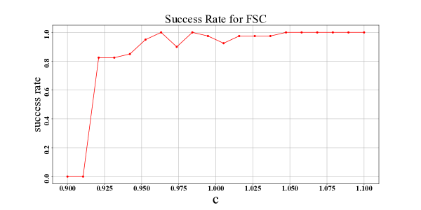
Figure 2. Numerical results for FSC on the Hidden Clique problem. For each $c$, 40 trials of the hidden clique problem are run with $n=1000$. The step of switching $0$ to $-1$ is omitted. The random graph in which the clique is embedded is $G(n,1/2)$. Reported are the fraction of trials for which the clique was recovered exactly with no mis-classifications of any vertex.

13.2. Clique partition

Let us consider the situation where one hides many cliques $X_{1},\dots,X_{r}$ of size $k_{1}\geq k_{2}\geq\dots\geq k_{r}$, which form a partition of the vertex set. The vertices of different cliques are connected with probability $1/2$, independently. The first task is to find the $i$th largest clique $X_{i}$, for any given $1\leq i\leq r$, given one instance of the random graph.

One can do this by finding all $X_{i}$ and then sorting them out. However, we can do the task directly by just computing the $i$th singular vector and clustering on its coordinates (the same way as in the last section). Before starting the main step of the algorithm , we change all zeros in the adjacency matrix to $-1$.

Algorithm 54 ($i$th clique).

Compute the $i$th singular vector. Let $x$ be the largest value of a coordinate and let $X_{i}$ be the set of all coordinates with value at least $x/2$.

One issue is that if $k_{i}=k_{i-1}$, then there is no way to differentiate $X_{i}$ from $X_{i-1}$. Thus, the hard instances for the problem are when $|k_{i}-k_{j}|$ are small in general. In what follows, we concentrate on that case, and assume that all $k_{i}$ are of order $n$. Our theorems enable us to find $X_{i}$ correctly under the assumption that $|k_{i}-k_{i\pm 1}|=\tilde{O}(1)$.

Theorem 55.

For any constant $c>0$ there is a constant $C$ such that the following holds. Assume that $k_{r}\geq cn$ and $k_{i}-k_{i+1}\geq C\log n$ for all $1\leq i\leq r$. Then with probability at least $.99$, Algorithm 54 recovers $X_{i}$ correctly, for any $1\leq i\leq r$.

In what follows, we illustrate the ideas through the case $i=1$. The analysis for a general $i$ is similar. Consider the leading eigenvector of $\tilde{A}=A+E$, where $A$ now consists of $r$ disjoint diagonal all-one blocks of sizes $k_{1},\dots,k_{r}$.

$$A=\begin{bmatrix}\mathbbm{1}_{k_{1}}\mathbbm{1}_{k_{1}}^{T}&0&\dots&0\\ 0&\mathbbm{1}_{k_{2}}\mathbbm{1}_{k_{2}}^{T}&0&\vdots\\ \vdots&0&\ddots&0\\ 0&\dots&0&\mathbbm{1}_{k_{r}}\mathbbm{1}_{k_{r}}^{T}\\ \end{bmatrix}$$

The leading eigenvalue of $A$ is $k_{1}$ and the leading eigenvector is

$$(1/\sqrt{k_{1}},\dots,1/\sqrt{k_{1}},0,\dots,0).$$

The next eigenvalue is $k_{2}$ and the gap $\delta_{1}=k_{1}-k_{2}$. Since the cliques partition the vertex set, $k_{1}\geq n/r$. The difference (compared to the previous section) is that, with probability $.99$, the $\ell_{2}$ error (from Theorem 3) is now bounded by

$$O\Big{[}\frac{1}{\delta_{1}}+\frac{\|E\|}{\sigma}+\frac{\|E\|^{2}}{\delta_{1}\sigma}\Big{]}=O\Big{[}\frac{1}{k_{1}-k_{2}}+\frac{\sqrt{n}}{k_{1}}+\frac{n}{k_{1}(k_{1}-k_{2})}\Big{]}=O\Big{[}\frac{1}{k_{1}-k_{2}}\Big{]}.$$

Since we assume that all $k_{i}=\Theta(n)$, the infinity norm of $U$ is $O(\frac{1}{\sqrt{n}})$. So, our Theorem 10 implies that with probability at least $.99$, the infinity norm bound for the first eigenvector is

$$O\Big{[}\frac{r\sqrt{\log n}}{(k_{1}-k_{2})\sqrt{n}}+\frac{\log n}{n}\Big{]}\leq\frac{1}{4k_{1}^{1/2}},$$

given that $(k_{1}-k_{2})/\sqrt{\log n}$ is bounded from below by a sufficiently large constant, proving the claim.

We found a simple, but effective, trick to reduce the general case (when the separation condition could be violated, such as when $k_{i}$ are all the same) to the situation in Theorem 55. We call this trick random truncation and it works as follows.

Random truncation. Select each vertex with probability $\rho:=n^{-1+\epsilon}$, independently, where $\epsilon$ is a small positive constant. Let $S$ be the set of selected vertices and $V^{\prime}=V\backslash S,X_{i}^{\prime}=X_{i}\backslash S,k_{i}^{\prime}=|X_{i}^{\prime}|$. If $k_{i}=\Theta(n)$ then $|X_{i}\cap S|$ is a binomial random variable $\chi$ with mean $k_{i}\rho=\Theta(n\rho)$ and standard deviation $\Theta(\sqrt{n\rho})=\Theta(n^{\epsilon/2})$. Since $\log n=o(n^{\epsilon/2})$, the following fact is obvious.

Fact 56.

(Separation Lemma) Consider the random variable $\chi$ above and let $\chi^{\prime}$ be its independent copy. Then for any given interval $I$ of length $O(\log n)$, with probability at least $1-o(1)$, $\chi-\chi^{\prime}\not\in I$.

By the union bound over all pairs $(i,j)$, it follows that with probability at least $1-o(1)$, $\min_{i\neq j}|k_{i}^{\prime}-k_{j}^{\prime}|=\omega(\log n)$. Thus, our separation condition holds on the subgraph spanned by $V^{\prime}$. We can now run our algorithm on the adjacency matrix of this graph to identify $X_{i}^{\prime}$. To finish, define $X_{i}$ as the union of $X_{i}^{\prime}$ with the vertices in $S$ which are connected to all the vertices in $X_{i}^{\prime}$.

Another natural task is to find all $X_{i}$, and we can complete this task by consecutive applications of the algorithm FSC from the last section. First, find $X_{1}$ (or more precisely $X_{1}^{\prime}$), then remove it from the graph. Then, find $X_{2}$ and continue in this way. Here is the formal description of the algorithm.

Algorithm 57 (Clique partition).

2. Define a set $S$ by choosing each vertex in $S$ with probability $\rho:=n^{-1+\epsilon}$. Let $V^{\prime}=V\backslash S$ and consider the graph spanned by $V^{\prime}$.

3. For $i=1,\dots,r-1$, run FSC to get $X_{i}^{\prime}$. Let $X^{\prime}_{r}=V^{\prime}\backslash\cup_{i=1}^{r-1}V_{i}$.

4. Define $X_{i}$ be the union of $X_{i}^{\prime}$ and the vertices of $S$ which are adjacent to all of $X_{i}$.

Theorem 58.

Assume that $k_{i}=\Theta(n)$ for all $1\leq i\leq r$. With probability at least $.9$, the Algorithm Clique Partition recovers $X_{1},\dots,X_{n}$ correctly.

13.3. Planted colorings

Finding a $r$ coloring of a graph is a notoriously hard problem, even when we know that the graph is $r$-colorable. A number of researchers have considered the random instance of this problem. One natural setting is as follows. Partition the vertex set $V$ into $r$ independent sets $X_{1},\dots,X_{r}$ of sizes $k_{1}\geq k_{2}\dots\geq k_{r}$ and then connect the vertices between different $X_{i}$ with probability $1/2$. The task is to recover the proper coloring from one instance of this random graph; see for instance [6], [13].

Notice that if we look at the complement graph, then this is exactly the problem considered in the previous section, as independent sets become cliques. Thus, we obtain

Theorem 59.

Assume that $k_{i}=\Theta(n)$ for all $1\leq i\leq r$. Then with probability at least $.9$, the algorithm in the last section recovers the planted coloring.

Remark 60.

In this and the previous problems, the constant $1/2$ again is not important, and can be replaced by a general density $p$. The condition that $k_{i}=\Theta(n)$ for all $i$ can also be weakened.

13.4. Hidden partition

We now consider a generalization of the problem in Section 13.2, where each clique $X_{i}$ is replaced by a random graph with edge density $p_{i}>1/2$. Similar to Section 13.2, the task is to locate a particular $X_{i}$ or all $X_{i}$ from one random instance of the graph.

Switch all $0$ in the adjacency matrix to $-1$. The resulting matrix $\tilde{A}$ can be decomposed into $A+E$, where $A$ now has the following form

$$A=\begin{bmatrix}(2p_{1}-1)\mathbbm{1}_{k_{1}}\mathbbm{1}_{k_{1}}^{T}&0&\dots&0\\ 0&(2p_{2}-1)\mathbbm{1}_{k_{2}}\mathbbm{1}_{k_{2}}^{T}&0&\vdots\\ \vdots&0&\ddots&0\\ 0&\dots&0&(2p_{r}-1)\mathbbm{1}_{k_{r}}\mathbbm{1}_{k_{r}}^{T}\\ \end{bmatrix}$$

The random matrix $E$ has the following form. The entry $e_{ij}$, $1\leq i\leq j\leq n$, is Rademacher ($\pm 1$) if $i$ and $j$ belong to different $X_{k}$. If they belong to the same $X_{k}$, then let $e_{ij}=(2-2p_{k})$ with probability $p_{k}$ and $-2p_{k}$ with probability $1-p_{k}$. It is easy to check that $\tilde{A}=A+E$ and that all entries of $E$ have zero-mean and are $2$-bounded.

Set $\rho_{i}:=2p_{i}-1$. The singular values of $A$ are $k_{1}\rho_{1},\dots,k_{r}\rho_{r}$. We replace the assumption $k_{1}\geq k_{2}\geq\dots\geq k_{r}$ by its weighted version $k_{1}\rho_{1}\geq k_{2}\rho_{2}\geq\dots\geq k_{r}\rho_{r}$. The leading singular value of $A$ is now $k_{1}\rho_{1}$, the second is $k_{2}\rho_{2}$ and the gap is $\delta_{1}=k_{1}\rho_{1}-k_{2}\rho_{2}$; the singular vector remains the same. If we follow the proof of Theorem 55, then the condition becomes

$$\frac{1}{k_{i}^{1/2}}\frac{r}{\delta_{i}}+\frac{\sqrt{\log n}}{k_{i}\rho_{1}}\leq C^{-1}\frac{1}{k_{i}^{1/2}}$$

for some sufficiently large constant $C$. This is equivalent to assuming that both $\delta_{i}$ and $\sqrt{k_{i}}\rho_{i}/\sqrt{\log n}$ are lower bounded by some sufficiently large constant $C$. The second one is equivalent to $\rho_{i}\geq C\sqrt{\log n/n}$ for some sufficiently large constant $C$.

Theorem 61.

For any constant $c_{1}$, there is a constant $C$ such that the following holds. Assume that $k_{1}\rho_{1}/k_{r}\rho_{r}$ is bounded from above by $c_{1}$. If $\delta_{i}\geq C\log n$ and $\rho_{i}\geq C\sqrt{\log n/n}$ then the $i$th clique algorithm recovers $X_{i}$ correctly with probability $.9$.

We can again apply the random truncation trick at the beginning to guarantee the separation condition. However, the application of this trick on this more general setting is slightly more technical than in the case of cliques, since it is less obvious how to assign the vertices from $S$ to $X_{i}^{\prime}$. To decide which $X_{i}^{\prime}$ a vertex $v\in S$ belongs to, we first choose a subset $Y_{i}\subset X_{i}^{\prime}$ so that all $Y_{i}$ has the same size $cn$ for some constant $c>0$. (This is doable because we assume that all $X_{i}$ have size $\Theta(n)$.) Let $i$ be the index where $v$ has the most edges connected to $Y_{i}$ and then add $v$ to $X_{i}^{\prime}$.

Notice that if $v\not\in X_{i}$, then the number of edges between $v$ and $Y_{i}$ has distribution $\chi_{0}=\operatorname{Binom}(.5,cn)$. If $v\in X_{i}$ then it has distribution $\chi_{i}=\operatorname{Binom}(p_{i},cn)$. If $p_{i}-.5:=\rho_{i}/2>C_{0}\sqrt{n\log n}$ for a sufficiently large constant $C_{0}$ (which may depend on $c$ and $r$, then with probability at least $.99$, $\chi_{i}\geq\chi_{0}$ for all $v\in S$ and $1\leq i\leq r$. This leads us to the following algorithm and theorem.

Algorithm 62 (Hidden partition).

2. Define a set $S$ by choosing each vertex in $S$ with probability $\rho:=n^{-1+\epsilon}$. Let $V^{\prime}=V\backslash S$ and consider the graph spanned by $V^{\prime}$.

3. For $i=1,\dots,r-1$, run FSC to get $X_{i}^{\prime}$. Let $X^{\prime}_{r}=V^{\prime}\backslash\cup_{i=1}^{r-1}V_{i}$.

4. Select subsets $Y_{i}\subset X_{i}^{\prime}$ such that $|Y_{i}|=cn$, for some properly chosen small constant $c>0$.

5. Define $X_{i}$ be the union of $X_{i}^{\prime}$ and those vertices $v$ of $S$ where $d_{i}(v)=\max_{j}d_{j}(v)$, where $d_{i}(v)$ is the number of neighbors of $v$ in $Y_{i}$ (break ties arbitrarily).

Theorem 63.

For any constant $c$ there are constants $c_{0},C$ such that the following holds. If $k_{i}\geq cn$ and $\rho_{i}\geq C\sqrt{\log n/n}$ for all $1\leq i\leq r$, then Algorithm Hidden Partition recovers all $X_{i}$ correctly with probability $.9$.

Remark 64.

The density $1/2$ again is not important, and can be replaced by a general density $q$.

Another well-known instance of this problem is the hidden bipartition problem. In this problem, $r=2$ and the vertex set is partitioned into two sets of equal size $n/2$. Draw edges with probability $p$ inside $X_{i}$ and $q<p$ between $X_{1}$ and $X_{2}$. The task is to recover the partition from one instance of the random graph. This particular case has been studied heavily by many researchers through 4 decades; see Table 2.

Bui, Chaudhuri, Leighton, Sipser ’84 [16]	min-cut method	$p=\Omega(1/n),q=o(n^{-1-4/((p+q)n)})$
Dyer, Frieze ’89 [35]	min-cut via degrees	$p-q=\Omega(1)$
Boppana ’87 [15]	spectral method	$(p-q)/\sqrt{p+q}=\Omega(\sqrt{\log(n)/n})$
Snijders, Nowicki ’97 [56]	EM algorithm	$p-q=\Omega(1)$
Jerrum, Sorkin ’98 [42]	Metropolis algorithm	$p-q=\Omega(n^{-1/6+\epsilon})$
Condon, Karp ’99 [28]	augmentation algorithm	$p-q=\Omega(n^{-1/2+\epsilon})$
Carson, Impagliazzo ’01 [14]	hill-climbing algorithm	$p-q=\Omega(n^{-1/2}\log^{4}n)$
Mcsherry ’01 [50]	spectral method	$(p-q)/\sqrt{p}\geq\Omega(\sqrt{\log(n)/n})$
Bickel, Chen ’09 [12]	N-G modularity	$(p-q)/\sqrt{p+q}=\Omega(\log(n)/\sqrt{n})$
Rohe, Chatterjee, Yu ’11 [55]	spectral method	$p-q=\Omega(1)$
Abbe, Bandeira, Hull ’14 [2]	maximum likelihood	$p-q=\Omega(\sqrt{\log(n)/n})$
Vu ’18 [59]	spectral method	$(p-q)/p^{1/2}=\Omega(\sqrt{\log(n)/n})$
Abbe, Fan, Wang, Zhong ’19 [4]	spectral method	$p-q=\Omega(\sqrt{\log(n)/n})$

Table 2. A recreation of the table in [2] surveying the hidden bipartition problem, with some recent additions.

In this case, our method (with some obvious modifications to replace $1/2$ by $q$) gives

Theorem 65.

If $p,q=\Theta(1)$, $p-q\geq C\sqrt{\log n/n}$ for all $1\leq i\leq r$, then Algorithm Hidden Partition recovers all $X_{i}$ correctly with probability $.9$.

The lower bound $\sqrt{\log n/n}$ is the current best on this problem; see [2]. From our analysis, it is clear that the same conclusion holds for equal partitions with any number of parts (more than 2). The condition $p,q=\Theta(1)$ can also be improved, and with $p$ tending to zero, it becomes $(p-q)/\sqrt{p}\geq C\sqrt{\log n/n}$.

14. Application: Exact Matrix Completion from Few Entries

In this section, we prove Theorem 23. Let us recall that $A$ is an integer matrix with rank $r=O(1)$, with entries bounded by an absolute constant (so $\left\lVert A\right\rVert_{\infty}=O(1)$). Let $S$ be the sampled version of $A$ where each entry is sampled (independently) with probability $p$, and the un-sampled entries are zeroed out. Then $\tilde{A}:=p^{-1}S$ is an unbiased estimate of $A$. We analyze the simple spectral algorithm in Section 14 to recover $A$ exactly from $\tilde{A}$. Set $W=[U,V]$, the concatenated matrix of $U$ and $V$, where $U$ and $V$ are the left and right singular vectors of $A$ respectively. Recall that we set $s:=\max_{i}\{i:\sigma_{i}\geq\frac{1}{16r}\|W\|_{\infty}^{-2}\}$, $\overline{\delta}=\inf_{i\leq s}\delta_{i}$, and $\tilde{s}=\max_{i}\{i:\tilde{\sigma}_{i}\geq\frac{1}{8r}\left\lVert W\right\rVert_{\infty}^{-2}\}$. Let $a=\max\{\sqrt{\left\lVert A\right\rVert_{\infty}},2\}.$ For concreteness, set $c$ to be the constant $(a+1)\times 2^{18}\times 7r^{3}$.

By the rounding step, in order to have exact recovery, we need to show that

$$\left\lVert A-B\right\rVert_{\infty}<\frac{1}{2}.$$

Let us consider the entry $A_{12}$. By the singular value decompositions of $A$ and $B$,

$$A_{12}=\sum_{i=1}^{r}\sigma_{i}u_{i1}v_{i2},\hskip 5.69054ptB_{12}=\sum_{i=1}^{\tilde{s}}\tilde{\sigma}_{i}\tilde{u}_{i1}\tilde{v}_{i2}.$$

Let $A_{\tilde{s}}$ be the best rank $\tilde{s}$ approximation of $A$. Thus, $A=A_{\tilde{s}}+\sum_{i=\tilde{s}+1}^{r}\sigma_{i}u_{i}u_{i}^{T}$. Write $A_{\tilde{s}ij}$ for the $ij$ entry of $A_{\tilde{s}}$. By the triangle inequality, we have

$$\begin{split}\lvert B_{12}-A_{12}\rvert&\leq\lvert B_{12}-A_{\tilde{s}12}\rvert+\lvert\sum_{i=\tilde{s}+1}^{r}\sigma_{i}u_{i1}v_{i2}\rvert\\ &=\Big{\lvert}\sum_{i=1}^{\tilde{s}}\tilde{\sigma}_{i}\tilde{u}_{i1}\tilde{v}_{i2}-\sum_{i=1}^{\tilde{s}}\sigma_{i}u_{i1}v_{i2}\Big{\rvert}+\lvert\sum_{i=\tilde{s}+1}^{r}\sigma_{i}u_{i1}v_{i2}\rvert.\end{split}$$ (145)

Bounding the second term on the RHS is fairly straightforward, and is handled in Lemma 67. The choice of the threshold $\tilde{s}$ plays an important role. Before stating the lemma, we will need the following tail bound on the norm of $E$. Its proof relies on a result from [10] and is given in Appendix D. This lemma will be used throughout this section.

Lemma 66.

There exists an absolute constant $C$ such that

$$\mathbb{P}\{\left\lVert E\right\rVert\geq C\sqrt{Np^{-1}}\}\leq N^{-3}.$$ (146)

For convenience, we define

$$\mathcal{E}:=\{\left\lVert E\right\rVert\leq C\sqrt{Np^{-1}}\},$$

where $C$ is the constant above.

Lemma 67.

With probability at least $1-N^{-3}$,

$$\lvert\sum_{i=\tilde{s}+1}^{r}\sigma_{i}u_{i1}v_{i2}\rvert\leq\frac{1}{4}.$$

In the next lemma, we bound the first term on the RHS of (145). This is where we use our refined bounds for the large $K$ case. As we have mentioned, unlike the clustering problem, $K$ can be quite large in the matrix completion setting.

Lemma 68.

Under the conditions of Theorem 23, with probability at least $1-3N^{-2}$,

$$\lvert B_{12}-A_{\tilde{s}12}\rvert<\frac{1}{4}.$$

Lemmas 67 and 68 applied to the RHS of (145) are enough to conclude the result of Theorem 23, because then the error will be strictly less than $\frac{1}{4}+\frac{1}{4}=\frac{1}{2}$, and will thus be rounded away. The choice of considering entry $(1,2)$ is arbitary; with probability $1-N^{-1}$, the bound holds for all of the entries. The remainder of the section is dedicated to proving Lemmas 67 and 68.

Proof of Lemma 67.

Suppose that $\mathcal{E}$, which has probability $1-N^{-3}$ by Lemma 66, occurs. Recall that $\tilde{s}=\max_{i}\{i:\tilde{\sigma}_{i}\geq\frac{\left\lVert W\right\rVert_{\infty}^{-2}}{8r}\}$. Therefore, for all $i\geq\tilde{s}+1$, it must be the case that $\tilde{\sigma}_{i}\leq\frac{1}{8r}\left\lVert W\right\rVert_{\infty}^{-2}.$ By Fact 25 and Lemma 66, for $i\geq\tilde{s}+1$,

$$\sigma_{i}\leq\tilde{\sigma}_{i}+\left\lVert E\right\rVert\leq\frac{\left\lVert W\right\rVert_{\infty}^{2}}{8r}+C\sqrt{Np^{-1}}.$$

By the density assumption, $p>N^{-1}\log^{4.03}N$. By the incoherence assumption, $\left\lVert W\right\rVert_{\infty}\leq cN^{-1/2}$. Therefore, $\sqrt{Np^{-1}}=o\Big{(}\left\lVert W\right\rVert_{\infty}^{-2}\Big{)}$. It follows that for $i\geq\tilde{s}+1$,

$$\sigma_{i}\leq\frac{\left\lVert W\right\rVert_{\infty}^{2}}{4r}.$$

We have

$$\begin{split}\lvert\sum_{i=\tilde{s}+1}^{r}\sigma_{i}u_{i1}v_{i2}\rvert&\leq\sum_{i=\tilde{s}+1}^{r}\sigma_{i}\lvert u_{i1}\rvert\lvert v_{i2}\rvert\\ &\leq\frac{\left\lVert W\right\rVert_{\infty}^{-2}}{4r}\sum_{i=\tilde{s}+1}^{r}\lvert u_{i1}\rvert\lvert v_{i2}\rvert.\end{split}$$ (147)

Because both $\lvert u_{i1}\rvert\leq\left\lVert W\right\rVert_{\infty}$ and $\lvert v_{il}\rvert\leq\left\lVert W\right\rVert_{\infty}$, it follows that

$$\begin{split}\lvert\sum_{i=\tilde{s}+1}^{r}\sigma_{i}u_{i1}v_{i2}\rvert\leq\frac{1}{4r}\sum_{i=\tilde{s}+1}^{r}1\leq\frac{1}{4}.\end{split}$$ (148)

∎

In order to establish Lemma 68, we need the following proposition and lemma.

Proposition 69.

Suppose that $\mathcal{E}$ occurs. Then, $\tilde{s}\leq s$.

Proof.

Suppose $\mathcal{E}$ occurs. Assume towards contradiction that $\tilde{s}>s$. By definition of $\tilde{s}$, this means that there are at least $s+1$ singular values of $\tilde{A}$ larger than $\frac{\left\lVert W\right\rVert_{\infty}^{-2}}{8r}$, so

$$\tilde{\sigma}_{s+1}\geq\frac{\left\lVert W\right\rVert_{\infty}^{-2}}{8r}.$$ (149)

By definition of $s$, $\sigma_{s+1}\leq\frac{\left\lVert W\right\rVert_{\infty}^{-2}}{16r}$. Therefore, by Fact 25,

$$\tilde{\sigma}_{s+1}\leq\sigma_{s+1}+\left\lVert E\right\rVert\leq\frac{\left\lVert W\right\rVert_{\infty}^{-2}}{16r}+C\sqrt{Np^{-1}}=\frac{\left\lVert W\right\rVert_{\infty}^{-2}}{16r}+o(\left\lVert W\right\rVert_{\infty}^{-2})<\frac{\left\lVert W\right\rVert_{\infty}^{-2}}{8r}.$$

where we use our previous observation that $\sqrt{Np^{-1}}=o(\left\lVert W\right\rVert_{\infty}^{-2})$. This is a contradiction with (149). ∎

Lemma 70.

Set $m_{\infty}(i)=\max\{\left\lVert\tilde{\mathbf{u}}_{i}-\mathbf{u}_{i}\right\rVert_{\infty},\left\lVert\tilde{\mathbf{v}}_{i}-\mathbf{v}_{i}\right\rVert_{\infty}\}$ and $m_{2}(i)=\max\{\left\lVert\tilde{\mathbf{u}}_{i}-\mathbf{u}_{i}\right\rVert_{2},\left\lVert\tilde{\mathbf{v}}_{i}-\mathbf{v}_{i}\right\rVert_{2}\}$. Under the conditions of Theorem 23, there exists a constant $c_{0}$ such that with probability at least $1-2N^{-2}$,

$$\sup_{i\leq s}m_{\infty}(i)\leq\frac{c_{0}\left\lVert W\right\rVert_{\infty}}{\log N}.$$ (150)

Proof of Lemma 68 given Lemma 70.

Recall that

$$\lvert B_{12}-A_{\tilde{s}12}\rvert=\Big{\lvert}\sum_{i=1}^{\tilde{s}}\tilde{\sigma}_{i}\tilde{u}_{i1}\tilde{v}_{i2}-\sum_{i=1}^{\tilde{s}}\sigma_{i}u_{i1}v_{i2}\Big{\rvert}.$$

Letting $\tilde{u}_{i1}=u_{i1}+\Delta u_{i1}$ and $\tilde{v}_{i2}=v_{i2}+\Delta v_{i2}$, we have

$$B_{12}=\sum_{i=1}^{\tilde{s}}\tilde{\sigma}_{i}[u_{i1}v_{i2}+u_{i1}\Delta v_{i2}+v_{i2}\Delta u_{i1}+\Delta u_{i1}\Delta v_{i2}].$$ (151)

Let $c_{0}$ be the constant from Lemma 70. Suppose $\mathcal{E}$ and $\{\sup_{i\leq s}m_{\infty}(i)\leq\frac{c_{0}}{\log N}\}$ both occur. By the lemma and the union bound, this happens with probability at least $1-3N^{-2}$. Since $\mathcal{E}$ occurs, $\tilde{s}\leq s$ by Proposition 69. It follows that

$$\lvert B_{12}-A_{\tilde{s}12}\rvert\leq\sum_{i=1}^{s}\lvert\tilde{\sigma}_{i}-\sigma_{i}\rvert\lvert u_{i1}v_{i2}\rvert+d,$$ (152)

where

$$d:=\sum_{i=1}^{s}\tilde{\sigma}_{i}[\lvert u_{i1}\rvert\lvert\Delta v_{i2}\rvert+\lvert v_{i2}\rvert\lvert\Delta u_{i1}\rvert+\lvert\Delta u_{i1}\rvert\lvert\Delta v_{i2}\rvert].$$

Observe that both $\lvert\Delta u_{i1}\rvert$ and $\lvert\Delta v_{i2}\rvert$ are bounded by $m_{\infty}(i)$. We consider the two terms on the RHS of (152) separately. For the first term, using Fact 25, $\lvert\tilde{\sigma}_{i}-\sigma_{i}\rvert\leq\left\lVert E\right\rVert$. Since $\lvert u_{i1}\rvert\lvert v_{i2}\rvert\leq\left\lVert W\right\rVert_{\infty}^{2}$, we have

$$\sum_{i=1}^{s}\lvert\tilde{\sigma}_{i}-\sigma_{i}\rvert\lvert u_{i1}v_{i2}\rvert\leq r\left\lVert E\right\rVert\left\lVert W\right\rVert_{\infty}^{2}$$ (153)

By the incoherence assumption, $\left\lVert W\right\rVert_{\infty}=O(N^{-1/2})$ so $\left\lVert W\right\rVert^{2}=O(N^{-1})$. Since $\mathcal{E}$ occurs,

$$\left\lVert E\right\rVert\leq C\sqrt{Np^{-1}}=o(N),$$

where the last equality uses the assumed lower bound for $p$, $p>\frac{\log^{4.03}N}{N}$. It follows that $\left\lVert E\right\rVert\left\lVert W\right\rVert_{\infty}^{2}=o(1)$.

$$\sum_{i=1}^{s}\lvert\tilde{\sigma}_{i}-\sigma_{i}\rvert\lvert u_{i1}v_{i2}\rvert=o(1).$$ (154)

Moving to the term $d$ on the RHS of (152), we bound for $i\leq s$, $\tilde{\sigma_{i}}\leq\sigma_{i}+\left\lVert E\right\rVert$ by Fact 25. By the signal-to-noise condition and the fact that $\mathcal{E}$ occurs, $\sigma_{s}>\left\lVert E\right\rVert$. Thus, $\sigma_{i}+\left\lVert E\right\rVert\leq 2\sigma_{i}$. Therefore,

$$\begin{split}d&=\sum_{i=1}^{s}\tilde{\sigma}_{i}[\lvert u_{i1}\rvert\lvert\Delta v_{i2}\rvert+\lvert v_{i2}\rvert\lvert\Delta u_{i1}\rvert+\lvert\Delta u_{i1}\rvert\lvert\Delta v_{i2}\rvert]\\ &\leq 2\sum_{i=1}^{s}\sigma_{i}[\lvert u_{i1}\rvert\lvert\Delta v_{i2}\rvert+\lvert v_{i2}\rvert\lvert\Delta u_{i1}\rvert+\lvert\Delta u_{i1}\rvert\lvert\Delta v_{i2}\rvert].\end{split}$$ (155)

Then, using the bounds $\lvert\Delta u_{i1}\rvert,\lvert\Delta v_{i1}\rvert\leq m_{\infty}(i)$ and $\lvert u_{i1}\rvert,\lvert v_{i1}\rvert\leq\left\lVert W\right\rVert_{\infty}$, we have

$$\begin{split}d&\leq 2\sum_{i=1}^{s}\sigma_{i}[2\left\lVert W\right\rVert_{\infty}m_{\infty}(i)+m_{\infty}^{2}(i)].\end{split}$$ (156)

Because $A$ has rank $r=O(1)$ and has $O(1)$ bounded entries, $\sigma_{1}=O(N)$. Since $\left\lVert W\right\rVert_{\infty}=O(N^{-1/2})$ by the incoherence assumption and $\sup_{i\leq s}m_{\infty}(i)=o(\left\lVert W\right\rVert_{\infty})$,

$$\begin{split}d=O(\sigma_{1}\left\lVert W\right\rVert_{\infty}\sup_{i\leq s}m_{\infty}(i))&=o(N\left\lVert W\right\rVert_{\infty}^{2})=o(1).\end{split}$$ (157)

(154) and (157) give that

$$\lvert B_{12}-A_{\tilde{s}12}\rvert=o(1)<\frac{1}{4},$$ (158)

for a large enough $N$. ∎

In order to prove Lemma 70, first establish that we can apply our refined (large $K$ case) results for the $\ell_{\infty}$ perturbation of singular vectors because the strong stability condition holds.

Lemma 71.

Recall that $a$ is the absolute constant $a=\max\{\sqrt{\left\lVert A\right\rVert_{\infty}},2\}.$ Under the conditions of Theorem 23, for all $i\leq s$, the singular values and gaps $(\sigma_{i},\delta_{i})$ are all $(\frac{c}{a+1},N^{-3},2)$ strongly stable under $E$.

Proof of Lemma 70 given Lemma 71.

Since the entries of $A$ are $O(1)$, $K=O(p^{-1})$. By Lemma 71 and the choice of $c$, the conditions for Theorem 19 to bound $m_{\infty}(i)$ hold with $\frac{c}{a+1}$, $\tau=N^{-3}$, $\nu=2$, and $K=O(p^{-1})$. Applying this for all $i\leq s$, using the fact that $\bar{\delta}$ is the minimum $\delta_{i}$ among the first $s$ singular values,

$$\sup_{i\leq s}m_{\infty}(i)=O\Bigg{(}\kappa_{s}\left\lVert W\right\rVert_{\infty}\Big{[}\sup_{i\leq s}m_{2}(i)+\frac{\left\lVert E\right\rVert}{\sigma_{s}}+\frac{\sqrt{\log N}}{p\overline{\delta}}\Big{]}+\frac{\kappa_{s}\sqrt{p^{-1}N}\left\lVert W\right\rVert_{\infty}\log N}{2\sigma_{s}}\Bigg{)},$$ (159)

with probability at least $1-N^{-2}$. Suppose in addition $\mathcal{E}$ holds, which happens with probability at least $1-N^{-3}$.

Recall that we wish to show that the LHS is less than $c\left\lVert W\right\rVert_{\infty}\log^{-1}N$. Let us start by bounding $\kappa_{s}$. We have shown that $\sigma_{1}=O(N)$. By definition of $s$, $\sigma_{s}\geq\frac{\left\lVert W\right\rVert_{\infty}^{-2}}{16r}=\Omega(N)$, where we also use the incoherence assumption. It follows that $\kappa_{s}=O(1)$. To handle the last term in the RHS of (159), we use that $\frac{\sqrt{Np^{-1}}}{\sigma_{s}}=O(\log^{-2.01}N)$ by the signal-to-noise assumption, so

$$\frac{\kappa_{s}\sqrt{p^{-1}N}\left\lVert W\right\rVert_{\infty}\log N}{2\sigma_{s}}=o(\left\lVert W\right\rVert_{\infty}\log^{-1}N).$$ (160)

For the remaining term, we first bound $\sup_{i\leq s}m_{2}(i)$. We appeal to the $\ell_{2}$ perturbation bounds of [52]. We adapt their results to our situation in Corollary 77 in Appendix B, which we can apply because $\bar{\delta}>cp^{-1}\log N$. This result gives that with probability at least $1-N^{-3}$,

$$\sup_{i\leq s}m_{2}(i)=O\Big{[}\frac{\sqrt{\log N}}{p\bar{\delta}}+\frac{\left\lVert E\right\rVert}{\sigma_{s}}+\frac{\left\lVert E\right\rVert^{2}}{\sigma_{s}\bar{\delta}}\Big{]}.$$ (161)

Using this bound and (160), (159) becomes

$$\sup_{i\leq s}m_{\infty}(i)=O\Bigg{(}\kappa_{s}\left\lVert W\right\rVert_{\infty}\Big{[}\frac{\sqrt{\log N}}{p\overline{\delta}}+\frac{\left\lVert E\right\rVert}{\sigma_{s}}+\frac{\left\lVert E\right\rVert^{2}}{\sigma_{s}\bar{\delta}}\Big{]}\Bigg{)}+o(\left\lVert W\right\rVert_{\infty}\log^{-1}N).$$ (162)

Since $\kappa_{s}=O(1)$, the proof of the lemma will be complete once we establish that there is a constant $c_{1}$ such that the sum of the three terms in the brackets is at most $O(c_{1}\log^{-1}N)$. Let us start with the third term in the square brackets, $\frac{\left\lVert E\right\rVert^{2}}{\sigma_{s}\bar{\delta}}$. Since $\mathcal{E}$ holds,

$$\left\lVert E\right\rVert^{2}=O(Np^{-1}).$$

By the gap assumption, $\bar{\delta}^{-1}p^{-1}=O(\frac{1}{\log N})$. Thus, since $\sigma_{s}=\Omega(N)$,

$$\left\lVert E\right\rVert^{2}\bar{\delta}^{-1}\sigma_{s}^{-1}=O(N\sigma_{s}^{-1}\bar{\delta}^{-1}p^{-1})=O(\bar{\delta}^{-1}p^{-1})=O(\log^{-1}N).$$

Moving to the first term in the square brackets in (162), we have just established that $\bar{\delta}^{-1}p^{-1}=O(\log^{-1}N)$. Lastly, for the second term in the square brackets in (162), $\left\lVert E\right\rVert\sigma_{s}^{-1}=o(\log^{-1}N)$. This is by the signal-to-noise assumption and because $\mathcal{E}$ occurs. Since all three terms are either $O(\log^{-1}N)$ or $o(\log^{-1}N)$, the existence of $c_{1}$ can be quickly inferred.

A quick inspection of the proof gives that the total probability of occurrence of the events considered is at least $1-2N^{-2}$.

∎

Proof of Lemma 71.

Recall that $T=\inf\{t>0:\mathbb{P}(\left\lVert E\right\rVert>t)\leq N^{-1/3}\}$. By Lemma 66, $T\leq C\sqrt{Np^{-1}}$, where $C$ is the absolute constant from the lemma. Recall that $\bar{\delta}$ is the smallest gap in the first $s$ singular values of $A$. We will use $\sigma_{s}$ and $\bar{\delta}$ to show that that the singular values and gaps $(\sigma_{i},\delta_{i})$ for $i\leq s$ satisfy the $(\frac{c}{a+1},N^{-3},2)$ strong stability condition. Let $1\leq i\leq s$.

We first verify the three conditions for $(\frac{c}{a+1},N^{-3},2)$ stability, and conclude with verifying strong stability. First, the signal-to-noise condition gives

$$\sigma_{i}\geq\sigma_{s}>c\sqrt{Np^{-1}}\log^{2.01}N,$$ (163)

which ensures that

$$\sigma_{i}\geq\sigma_{s}>c\sqrt{Np^{-1}}\log^{2.01}N>\frac{c}{2}T\geq\frac{c}{a+1}T.$$

This shows that condition $(a)$ in Definition 8 holds for $(\sigma_{i},\delta_{i})$ with $\frac{c}{a+1}$ and $\tau=N^{-3}$.

Next, recall the gap condition

$$\bar{\delta}>cp^{-1}\log N.$$ (164)

In order to verify $(c)$ of Definition 8, we will show that

$$\bar{\delta}>\frac{c}{2}T\kappa_{i}\left\lVert W\right\rVert_{\infty},$$ (165)

which will imply $\delta_{i}>\frac{c}{a+1}T\kappa_{i}\left\lVert W\right\rVert_{\infty}$, as desired. Because $\kappa_{s}=O(1)$, the bound on $T$ implies

$$T\kappa_{i}\left\lVert W\right\rVert_{\infty}=O(\sqrt{p^{-1}}\sqrt{N}\left\lVert W\right\rVert_{\infty})=O(\sqrt{p^{-1}})$$

by the incoherence assumption. Thus, (165) holds by (164).

We examine $(b)$ in Definition 8, the final condition to verify $(\frac{c}{a+1},N^{-3},2)$ stability. Recall that $K$ is the bound for the absolute value of the entries of $E$. Observe that $K\leq\left\lVert A\right\rVert_{\infty}p^{-1}$. Since $\nu=2$, we must show that

$$\delta_{i}>\frac{c}{a+1}\Big{(}K\log N+\frac{T^{2}}{\sigma_{s}}\Big{)}.$$ (166)

Since $T\leq C\sqrt{Np^{-1}}$, it is sufficient to show that

$$\bar{\delta}>\frac{c}{a+1}\Big{(}K\log N+C^{2}\frac{Np^{-1}}{\sigma_{s}}\Big{)}.$$ (167)

Equation (164) implies that

$$\bar{\delta}>cp^{-1}\log N=\frac{c}{\left\lVert A\right\rVert_{\infty}}\left\lVert A\right\rVert_{\infty}p^{-1}\log N\geq\frac{c}{\left\lVert A\right\rVert_{\infty}}K\log N\geq\frac{c}{a}K\log N.$$

Since $\sigma_{s}=\Omega(N)$, $\frac{C^{2}Np^{-1}}{\sigma_{s}}=o(K\log N)$ because $p>N^{-1}\log N$. Therefore,

$$\bar{\delta}>\frac{c}{a}K\log N>\frac{c}{a+1}\Big{(}K\log N+C^{2}\frac{Np^{-1}}{\sigma_{s}}\Big{)}$$

as desired.

Having established $(\frac{c}{a+1},N^{-3},2)$ stability, we conclude with the verification of strong stability. The signal to noise condition, equation (163), implies that

$$\sigma_{i}\geq\sigma_{s}>\frac{c}{\sqrt{\left\lVert A\right\rVert_{\infty}}}\sqrt{N\left\lVert A\right\rVert_{\infty}p^{-1}}\log^{2.01}N\geq\frac{c}{\sqrt{\left\lVert A\right\rVert_{\infty}}}\sqrt{NK}\log^{2.01}N\geq\frac{c}{a+1}\sqrt{NK}\log^{2.01}N.$$ (168)

Thus, the conditions for strong stability in Definition 12 are satisfied for $(\sigma_{i},\delta_{i})$ with $\frac{c}{a+1}$, $\tau=N^{-3}$, and $\nu=2$. ∎

Appendix A Perturbation of Singular values

We begin with the definition of the concentration property. The authors of [52] state that a square matrix $E$ satisfies the $(C,c,\gamma)$ concentration property if for all unit vectors $\mathbf{u},\mathbf{v}\in\mathbb{R}^{n}$, and $t>0$,

$$\mathbb{P}(\lvert\mathbf{u}^{T}E\mathbf{v}\rvert>t)\leq C\exp(-ct^{\gamma}).$$ (169)

By using Hoeffding’s inequality, they show that if $K\geq 1$ and $E$ is an $n\times n$ symmetric matrix with independent, $K$ bounded entries, then

$$\mathbb{P}(\lvert\mathbf{u}^{T}E\mathbf{v}\rvert>t)\leq 2\exp(-\frac{1}{8K^{2}}t^{2})$$ (170)

In other words, $E$ satisfies the $(2,\frac{1}{8K^{2}},2)$-concentration property.

A key ingredient in the analysis is the singular values of the perturbed matrices $A^{\{l\}}$ and $\tilde{A}$. It is very easy to verify that if $E$ is a symmetric random matrix with independent, K- bounded entries, then for all $l$, $E^{\{l\}}$ has the $(2,\frac{1}{8K^{2}},2)$ concentration property as well. Therefore, the results derived in [52] for the perturbation of the singular values applies to $A^{\{l\}}$ for all $l$.

The main result for the perturbation of singular values in [52] is the following theorem.

Theorem 72.

Suppose that $E$ is $(C,c,\gamma)$ concentrated. Suppose that $A$ has rank $r$, and let $1\leq i\leq r$ be an integer. Then, for any $t\geq 0$,

$$\tilde{\sigma}_{j}\geq\sigma_{j}-t$$ (171)

with probability at least

$$1-2C9^{i}\exp\Big{(}-c\frac{t^{\gamma}}{4^{\gamma}}\Big{)}$$ (172)

and

$$\tilde{\sigma}_{i}\leq\sigma_{i}+tr^{1/\gamma}+2\sqrt{i}\frac{\left\lVert E\right\rVert^{2}}{\tilde{\sigma}_{i}}+i\frac{\left\lVert E\right\rVert^{3}}{\tilde{\sigma}^{2}_{i}}$$ (173)

with probability at least

$$1-2C9^{2r}\exp\Big{(}-cr\frac{t^{\gamma}}{4^{\gamma}}\Big{)}.$$ (174)

Theorem 30 follows from Theorem 72 and the fact that a symmetric, $K$ bounded random matrix with independent (above the diagonal) entries satisfies the $(2,\frac{1}{8K^{2}},2)$ concentration property.

Appendix B $\ell_{2}$ Perturbation of Eigenvectors

Theorem 73 ([52]).

Suppose that $E$ is $(C,c,\gamma)$ concentrated for a trio of constants $(C,c,\gamma)$ and suppose that $A$ has rank $r$. Then, for any $t>0$,

$$\left\lVert\tilde{\mathbf{u}}_{1}-\mathbf{u}_{1}\right\rVert_{2}\leq 8\Big{(}\frac{tr^{1/\gamma}}{\delta}+\frac{\left\lVert E\right\rVert}{\sigma_{1}}+\frac{\left\lVert E\right\rVert^{2}}{\delta\sigma_{1}}\Big{)}$$ (175)

with probability at least

$$1-54C\exp\Big{(}-c\frac{\delta^{\gamma}}{8^{\gamma}}\Big{)}-2C9^{2r}\exp\Big{(}-cr\frac{t^{\gamma}}{4^{\gamma}}\Big{)}.$$ (176)

Recall that a symmetric $E$ with independent, mean zero, $K$ bounded entries satisfies the $(2,\frac{1}{8K^{2}},2)$-concentration property. We will be considering only such matrices $E$ in what follows. Applying Theorem 73 gives the following theorem.

Theorem 74.

Let $E$ be a random, $K$-bounded, symmetric matrix with independent entries above the diagonal. For any $t>0$,

$$\left\lVert\tilde{\mathbf{u}}_{1}-\mathbf{u}_{1}\right\rVert_{2}\leq 8\Big{(}\frac{tr^{1/2}}{\delta}+\frac{\left\lVert E\right\rVert}{\sigma_{1}}+\frac{\left\lVert E\right\rVert^{2}}{\delta\sigma_{1}}\Big{)}$$ (177)

with probability at least

$$1-108\exp\Big{(}-\frac{\delta^{2}}{8^{3}K^{2}}\Big{)}-4\times 9^{2r}\exp\Big{(}-r\frac{t^{2}}{128K^{2}}\Big{)}.$$ (178)

As a consequence, if $\frac{\delta}{K\sqrt{8^{3}}}=\tau$, then for all $t\geq 0$, with probability at least $1-108\exp(-\tau^{2})-4*9^{2r}\exp\Big{(}-t\Big{)}$,

$$\left\lVert\tilde{\mathbf{u}}_{1}-\mathbf{u}_{1}\right\rVert_{2}\leq 8\Big{(}\frac{K\sqrt{128}t}{\delta}+\frac{\left\lVert E\right\rVert}{\sigma_{1}}+\frac{\left\lVert E\right\rVert^{2}}{\delta\sigma_{1}}\Big{)}$$ (179)

They also obtain the following recursive result for the perturbation of the remaining eigenvectors.

Theorem 75.

Assume that $E$ is $(C,c,\gamma)$ concentrated. Suppose that $A$ has rank $r$, and let $1\leq i\leq r$ be an integer. Then for any $t>0$,

$$\left\lVert\mathbf{u}_{i}-\tilde{\mathbf{u}}_{i}\right\rVert_{2}\leq 16\Bigg{[}\sum_{j=1}^{i-1}\left\lVert\tilde{\mathbf{u}}_{j}-\mathbf{u}_{j}\right\rVert_{2}+\frac{tr^{1/\gamma}}{\delta_{j}}+\frac{\left\lVert E\right\rVert}{\sigma_{j}}+\frac{\left\lVert E\right\rVert^{2}}{\sigma_{j}\delta_{j}}\Bigg{]}$$ (180)

with probability at least

$$1-6C9^{i}\exp\Big{(}-c\frac{\delta_{j}^{\gamma}}{8^{\gamma}}\Big{)}-2C9^{2r}\exp\Big{(}-cr\frac{t^{\gamma}}{4^{\gamma}}\Big{)}$$ (181)

Fix $1\leq s\leq r$. $s$ represents a cutoff point beyond which the eigenvectors are not of interest. Let $\epsilon_{j}(t):=16\Big{(}\frac{tr^{1/\gamma}}{\delta_{j}}+\frac{\left\lVert E\right\rVert}{\sigma_{j}}+\frac{\left\lVert E\right\rVert^{2}}{\sigma_{j}\delta_{j}}\Big{)}$. By taking the union bound over the first $s$ singular vectors and iterating this recursive bound, and letting $\overline{\delta}$ be the smallest gap in the first $s$ singular values, we obtain

Theorem 76.

For all $i\leq s$, and $t>0$,

$$\left\lVert\tilde{\mathbf{u}}_{i}-\mathbf{u}_{i}\right\rVert_{2}\leq\sum_{j=1}^{i}[\sum_{k=0}^{i-j}16^{k}]\epsilon_{j}(t)$$ (182)

with probability at least

$$1-6sC9^{s}\exp\Big{(}-c\frac{\bar{\delta}^{\gamma}}{8^{\gamma}}\Big{)}-2Cs9^{2r}\exp\Big{(}-cr\frac{t^{\gamma}}{4^{\gamma}}\Big{)}.$$ (183)

As a consequence, letting $\tau=\frac{\overline{\delta}}{K\sqrt{8^{3}}}$ if $E$ is symmetric and $K$-bounded with independent entries, there exists $C$ depending only on $s$ such that with probability at least $1-C[\exp(-\tau^{2})-9^{2r}\exp(-t)]$,

$$\sup_{i\leq s}\left\lVert\tilde{\mathbf{u}}_{i}-\mathbf{u}_{i}\right\rVert_{2}\leq C\Big{(}\frac{Kt}{\overline{\delta}}+\frac{\left\lVert E\right\rVert}{\sigma_{s}}+\frac{\left\lVert E\right\rVert^{2}}{\overline{\delta}\sigma_{s}}\Big{)},$$ (184)

for any $t>0$. In the rectangular case, where $A$ is an $m\times n$ matrix, and when $r=O(1)$, we derive the following corollary using the standard symmetrization trick. We encounter this setting in the matrix completion problem. Let $N=m+n$.

Corollary 77.

If $r=O(1)$ and $\overline{\delta}>400K\sqrt{\log N}$, with probability at least $1-N^{-3}$, we have

$$\sup_{i\leq s}\max\{\left\lVert\tilde{\mathbf{u}}_{i}-\mathbf{u}_{i}\right\rVert_{2},\left\lVert\tilde{\mathbf{v}}_{i}-\mathbf{v}_{i}\right\rVert_{2}\}=O\Big{(}\frac{Kt}{\overline{\delta}}+\frac{\left\lVert E\right\rVert}{\sigma_{s}}+\frac{\left\lVert E\right\rVert^{2}}{\overline{\delta}\sigma_{s}}\Big{)}.$$ (185)

Appendix C Results for Section 12

Lemma 78.

Let $Y\in\overline{\mathcal{L}_{\{\},l}}$ holds. Then,

$$\begin{split}\mathbb{P}(\mathcal{I}^{\prime}_{l}\lvert E^{\{l\}}=Y)&\leq 2\exp(-c_{2}\log n).\end{split}$$ (186)

Proof of Proposition 50 given the lemma..

The proposition follows immediately from the lemma once we observe that

$$\mathbb{P}(\mathcal{I}_{l}^{\prime}\cap\overline{\mathcal{L}_{\{\},l}})\leq\sup_{Y\in\overline{\mathcal{L}_{\{\},l}}}\mathbb{P}(\mathcal{I}_{l}^{\prime}|E^{\{l\}}=Y)\leq 2\exp(-c_{2}\log n).$$

∎

Proof of Lemma 78.

We are looking for a bound of

$$\mathbb{P}(\mathcal{I}^{\prime}_{l}|E^{\{l\}}=Y)=\mathbb{P}\{\lvert\langle\mathbf{u}^{\{l\}}_{i},\mathbf{x}(l)\rangle\rvert\geq c_{2}\sqrt{2Kn}f_{j+1}\log n\Big{\lvert}E^{\{l\}}=Y\}.$$

The lemma only considers realizations $Y$ of $E^{\{l\}}$ satisfying $\left\lVert\mathbf{u}^{\{l\}}_{i}\right\rVert_{\infty}\leq f_{1}$. Recall that $\mathbf{x}(l)$ is essentially the $l$th row of $E$ and $l\in\beta$. Therefore, conditional on such $E^{\{l\}}$, $\mathbf{u}^{\{l\}}_{i}$ is a deterministic unit vector whose entries have absolute value at most $f_{1}$. The only randomness in each event thus comes from $\mathbf{x}(l)$. It follows that the inner product $\langle\mathbf{u}^{\{l\}}_{i},\mathbf{x}(l)\rangle$, conditional on $E^{\{l\}}$, is the sum of independent, $Kf_{1}$ bounded, mean zero random variables $x_{k}u^{\{l\}}_{ik}$. Thus, this quantity can be bounded with Bernstein’s inequality. We are applying Bernstein’s inequality conditionally, so we also need to find a bound for the sum of the conditional second moments of the $x_{k}u^{\{l\}}_{ik}$. Since $\mathbf{u}^{\{l\}}_{i}$ is deterministic when we condition on $E^{\{l\}}$, and $\mathbf{x}(l)$ is independent of $E^{\{l\}}$, we have

$$\sum_{k=1}^{n}\mathbb{E}[x_{k}^{2}u^{\{l\}2}_{ik}|E^{\{l\}}=Y]=\sum_{k=1}^{n}u^{\{l\}2}_{ik}\mathbb{E}[x_{k}^{2}]\leq K\sum_{k=1}^{n}u^{\{l\}2}_{ik}=K.$$ (187)

For the inequality, we use that the second moments of the entries of $E$ are at most $K$ by Assumption 13. Applying Bernstein’s inequality (Lemma 29) then gives us that

$$\begin{split}\mathbb{P}\Big{\{}\lvert\langle\mathbf{u}^{\{l\}}_{i},\mathbf{x}(l)\rangle\rvert>t|E^{\{l\}}=Y\Big{\}}&\leq 2\exp\Big{(}\frac{-t^{2}/2}{\sum_{k=1}^{n}\mathbb{E}[x^{2}_{k}u^{\{l\}2}_{ik}|E^{\{l\}}=Y]+Kf_{1}t/3}\Big{)}\\ &\leq 2\exp\Big{(}\frac{-t^{2}/2}{K+Kf_{1}t/3}\Big{)}.\end{split}$$ (188)

Set $t=c_{2}\sqrt{2Kn}f_{1}\log n$. Since $n^{-1/2}\leq\left\lVert U\right\rVert_{\infty}\leq f_{1}$, we obtain that $K\leq Knf_{1}^{2}$. Thus, using this bound for the first term in the denominator of the RHS of (188),

$$\begin{split}\mathbb{P}\Big{\{}\lvert\langle\mathbf{u}^{\{l\}}_{i},\mathbf{x}(l)\rangle\rvert>c_{2}\sqrt{2Kn}f_{1}\log n\Big{|}E^{\{l\}}=Y\Big{\}}&\leq 2\exp\Big{(}\frac{-c_{2}^{2}Knf_{1}^{2}\log^{2}n}{Knf_{1}^{2}+\frac{\sqrt{2}c_{2}}{3}Kf^{2}_{1}\sqrt{Kn}\log n}\Big{)}\\ &\leq 2\exp\Big{(}\frac{-c_{2}^{2}Knf_{1}^{2}\log^{2}n}{Knf_{1}^{2}+\frac{\sqrt{2}c_{2}}{3}Kf_{1}^{2}n\log n}\Big{)}\\ &\leq 2\exp(-c_{2}\log n).\end{split}$$ (189)

In the second line, we used that $K\leq n$ by Assumption 13. ∎

Appendix D Proof of Lemma 66

In this section, we bound the spectral norm of the matrix $E$ from the matrix completion problem. We will use the following result from [10], which is a tail bound for the norm of $K$ bounded random matrices with independent entries.

Theorem 79 (Remark 3.13 in [10]).

Let $X$ be a symmetric, mean zero $n\times n$ random matrix whose entries above the diagonal are independent. Suppose the entries of $X$, $\xi_{ij}$, are $K$ bounded random variables. Let

$$v=\max_{i}\sum_{j}\mathbb{E}[\xi_{ij}^{2}].$$

Then there exists a universal constant $c>0$ such that for any $t\geq 0$,

$$\mathbb{P}\{\left\lVert E\right\rVert\geq 4\sqrt{v}+t\}\leq n\exp\Big{(}-\frac{t^{2}}{cK^{2}}\Big{)}.$$

Proof of Lemma 66.

Recall that $E$ is an $m\times n$ random matrix with independent, $K$ bounded entries, where $K=O(p^{-1})$. Form the symmetrization of $E$ as

$$S=S(E)=\begin{bmatrix}0&E\\ E^{T}&0\end{bmatrix}.$$

$S$ is a symmetric $N\times N$ random matrix satisfying the conditions of Theorem 79. It is easy to check that $\left\lVert E\right\rVert\leq\left\lVert S\right\rVert$. Let the entries of $S$ be given by $s_{ij}$. We need to calculate $v=\max_{i}\sum_{j}\mathbb{E}[s_{ij}^{2}]$ to apply the theorem. Recall that in the matrix completion setting, the entries of $E$ have second moment at most $K$. It follows that $\mathbb{E}[s_{ij}^{2}]\leq K$, so $v\leq NK$.

By Theorem 79,

$$\mathbb{P}\{\left\lVert S\right\rVert\geq 4\sqrt{NK}+t\}\leq N\exp\Big{(}\frac{-t^{2}}{cK^{2}}\Big{)}.$$ (190)

Set $t=K\sqrt{4c\log N}$. It follows that

$$\mathbb{P}\{\left\lVert S\right\rVert\geq 4\sqrt{NK}+K\sqrt{4c\log N}\}\leq N\exp\Big{(}-4\log N\Big{)}.$$ (191)

Since $\left\lVert E\right\rVert\leq\left\lVert S\right\rVert$,

$$\mathbb{P}\{\left\lVert E\right\rVert\geq 4\sqrt{NK}+\sqrt{4cK\log N}\}\leq N^{-3}.$$ (192)

Recall that $K=O(p^{-1})$. Under the assumptions of Theorem 23, $p>\frac{\log N}{N}$, so $\sqrt{K\log N}=o(\sqrt{N})$.

It follows that there exists an absolute constant $C$ such that

$$\mathbb{P}\{\left\lVert E\right\rVert\geq C\sqrt{NK}\}\leq N^{-3}.$$ (193)

∎

References

- [1] Emmanuel Abbe “Community Detection and Stochastic Block Models: Recent Developments” In Journal of Machine Learning Research 18.177, 2018, pp. 1–86
- [2] Emmanuel Abbe, Afonso S. Bandeira and Georgina Hall “Exact Recovery in the Stochastic Block Model” In IEEE Transactions on Information Theory 62.1, 2016, pp. 471–487
- [3] Emmanuel Abbe, Jianqing Fan and Kaizheng Wang “An theory of PCA and spectral clustering” In The Annals of Statistics 50, 2022
- [4] Emmanuel Abbe, Jianqing Fan, Kaizheng Wang and Yiqiao Zhong “Entrywise eigenvector analysis of random matrices with low expected rank” In Annals of Statistics 48.3 Institute of Mathematical Statistics, 2020, pp. 1452–1474
- [5] Joshua Agterberg, Zachary Lubberts and Carey E. Priebe “Entrywise Estimation of Singular Vectors of Low-Rank Matrices With Heteroskedasticity and Dependence” In IEEE Transactions on Information Theory 68, 2021, pp. 4618–4650
- [6] Noga Alon and Nabil Kahale “A Spectral Technique for Coloring Random 3-Colorable Graphs” In Proceedings of the Twenty-Sixth Annual ACM Symposium on Theory of Computing, STOC ’94 Montreal, Quebec, Canada: Association for Computing Machinery, 1994, pp. 346–355
- [7] Noga Alon, Michael Krivelevich and Benny Sudakov “Finding a Large Hidden Clique in a Random Graph” In Proceedings of the Ninth Annual ACM-SIAM Symposium on Discrete Algorithms, SODA ’98 San Francisco, California, USA: Society for IndustrialApplied Mathematics, 1998, pp. 594–598
- [8] Noga Alon and Joel H. Spencer “The Probabilistic Method” Wiley Publishing, 2016
- [9] Marco Avella-Medina, Heather S Battey, Jianqing Fan and Quefeng Li “Robust estimation of high-dimensional covariance and precision matrices” In Biometrika 105.2, 2018, pp. 271–284
- [10] Afonso S. Bandeira and Ramon Handel “Sharp nonasymptotic bounds on the norm of random matrices with independent entries” In The Annals of Probability 44.4 Institute of Mathematical Statistics, 2016, pp. 2479–2506
- [11] Zhigang Bao, Xiucai Ding and Ke Wang “Singular vector and singular subspace distribution for the matrix denoising model” In The Annals of Statistics 49.1, 2021
- [12] Peter J. Bickel and Aiyou Chen “A nonparametric view of network models and Newman–Girvan and other modularities” In Proceedings of the National Academy of Sciences 106, 2009, pp. 21068–21073
- [13] Avrim Blum and Joel Spencer “Coloring Random and Semi-Random k-Colorable Graphs” In J. Algorithms 19.2 USA: Academic Press, Inc., 1995, pp. 204–234
- [14] B. Bollobás and A.. Scott “MAX-CUT for Random Graphs with a Planted Partition” In Comb. Probab. Comput. 13.4–5 USA: Cambridge University Press, 2004, pp. 451–474
- [15] Ravi B. Boppana “Eigenvalues and graph bisection: An average-case analysis” In 28th Annual Symposium on Foundations of Computer Science (sfcs 1987), 1987, pp. 280–285
- [16] T. N. Bui, S. Chaudhuri, F. T. Leighton and M. Sipser “Graph bisection algorithms with good average case behavior” In Combinatorica 7.2 Janos Bolyai Mathematical Society, 1987, pp. 171–191
- [17] Changxiao Cai et al. “Subspace estimation from unbalanced and incomplete data matrices: statistical guarantees” In The Annals of Statistics 49.2 Institute of Mathematical Statistics, 2021, pp. 944–967
- [18] Emmanuel J. Candes and Michael B. Wakin “An Introduction To Compressive Sampling” In IEEE Signal Processing Magazine 25.2, 2008, pp. 21–30
- [19] Emmanuel Candès and Benjamin Recht “Exact Matrix Completion via Convex Optimization” In Commun. ACM 55.6 New York, NY, USA: Association for Computing Machinery, 2012, pp. 111–119
- [20] Emmanuel J. Candès and Yaniv Plan “Matrix Completion With Noise” In Proceedings of the IEEE 98, 2009, pp. 925–936
- [21] Emmanuel J. Candès and Terence Tao “The Power of Convex Relaxation: Near-Optimal Matrix Completion” In IEEE Trans. Inf. Theor. 56.5 IEEE Press, 2010, pp. 2053–2080
- [22] J Cape, M Tang and C E Priebe “Signal-plus-noise matrix models: Eigenvector Deviations and fluctuations” In Biometrika 106.1, 2019, pp. 243–250
- [23] Joshua Cape, Minh Tang and Carey E. Priebe “The two-to-infinity norm and singular subspace geometry with applications to high-dimensional statistics” In The Annals of Statistics, 2017
- [24] Sourav Chatterjee “Matrix estimation by Universal Singular Value Thresholding” In The Annals of Statistics 43.1 Institute of Mathematical Statistics, 2015
- [25] Yuxin Chen, Yuejie Chi, Jianqing Fan and Cong Ma “Spectral Methods for Data Science: A Statistical Perspective” In Foundations and Trends in Machine Learning 14.5 Now Publishers, 2021, pp. 566–806
- [26] Yuxin Chen et al. “Noisy Matrix Completion: Understanding Statistical Guarantees for Convex Relaxation via Nonconvex Optimization” In SIAM Journal on Optimization 30.4, 2020, pp. 3098–3121
- [27] Chen Cheng, Yuting Wei and Yuxin Chen “Tackling Small Eigen-Gaps: Fine-Grained Eigenvector Estimation and Inference Under Heteroscedastic Noise” In IEEE Trans. Inf. Theor. 67.11 IEEE Press, 2021, pp. 7380–7419
- [28] Anne Condon and Richard M. Karp “Algorithms for graph partitioning on the planted partition model” In Random Struct. Algorithms, 1999
- [29] Chandler Davis and W.. Kahan “The Rotation of Eigenvectors by a Perturbation. III” In SIAM Journal on Numerical Analysis 7.1 Society for IndustrialApplied Mathematics, 1970, pp. 1–46
- [30] Yael Dekel, Ori Gurel-Gurevich and Yuval Peres “Finding Hidden Cliques in Linear Time with High Probability” In 2011 Proceedings of the Workshop on Analytic Algorithmics and Combinatorics (ANALCO), pp. 67–75
- [31] Peter B. Denton, Stephen J. Parke, Terence Tao and Xining Zhang “Eigenvectors from eigenvalues: A survey of a basic identity in linear algebra” In Bulletin, new series, of the American Mathematical Society 59.1, 2021
- [32] Peter B. Denton, Stephen J. Parke and Xining Zhang “Neutrino oscillations in matter via eigenvalues” In Phys. Rev. D 101 American Physical Society, 2020, pp. 093001
- [33] Lijun Ding and Yudong Chen “The Leave-one-out Approach for Matrix Completion: Primal and Dual Analysis” In IEEE Transactions on Information Theory PP, 2018
- [34] Petros Drineas et al. “Clustering Large Graphs via the Singular Value Decomposition: Theoretical Advances in Data Clustering (Guest Editors: Nina Mishra and Rajeev Motwani)” In Machine Learning 56, 2004
- [35] M.. Dyer and A.. Frieze “The Solution of Some Random NP-Hard Problems in Polynomial Expected Time” In J. Algorithms 10.4 USA: Academic Press, Inc., 1989, pp. 451–489
- [36] Justin Eldridge, Mikhail Belkin and Yusu Wang “Unperturbed: spectral analysis beyond Davis-Kahan” In Proceedings of Algorithmic Learning Theory 83, Proceedings of Machine Learning Research PMLR, 2018, pp. 321–358
- [37] Jianqing Fan, Weichen Wang and Yiqiao Zhong “An Eigenvector Perturbation Bound and Its Application to Robust Covariance Estimation” In Journal of Machine Learning Research 18, 2016
- [38] Uriel Feige and Robert Krauthgamer “Finding and Certifying a Large Hidden Clique in a Semirandom Graph” In Random Struct. Algorithms 16.2 USA: John Wiley & Sons, Inc., 2000, pp. 195–208
- [39] Uriel Feige and Eran.. Ofek “Spectral techniques applied to sparse random graphs” In Random Structures & Algorithms 27, 2005
- [40] Uriel Feige and Dorit Ron “Finding hidden cliques in linear time” In Discrete Mathematics & Theoretical Computer Science DMTCS Proceedings vol. AM, 21st International Meeting on Probabilistic, Combinatorial, and Asymptotic Methods in the Analysis of Algorithms (AofA’10), 2010
- [41] W. Fernandez de la Vega “MAX-CUT has a randomized approximation scheme in dense graphs” In Random Structures & Algorithms 8.3, 1996, pp. 187–198
- [42] Mark Jerrum and Gregory B. Sorkin “The Metropolis Algorithm for Graph Bisection” In Discret. Appl. Math. 82, 1998, pp. 155–175
- [43] Ravindran Kannan and Santosh Vempala “Spectral Algorithms” In Foundations and Trends in Theoretical Computer Science 4, 2009, pp. 157–288
- [44] Raghunandan H. Keshavan, Andrea Montanari and Sewoong Oh “Matrix Completion From a Few Entries” In IEEE Transactions on Information Theory 56.6, 2010, pp. 2980–2998
- [45] Raghunandan H. Keshavan, Andrea Montanari and Sewoong Oh “Matrix Completion from Noisy Entries” In Journal of Machine Learning Research 11.69, 2010, pp. 2057–2078
- [46] Vladimir Koltchinskii and Dong Xia “Perturbation of linear forms of singular vectors under Gaussian noise” In High Dimensional Probability VII, 2016, pp. 397–423
- [47] Yehuda Koren, Robert Bell and Chris Volinsky “Matrix Factorization Techniques for Recommender Systems” In Computer 42.8, 2009, pp. 30–37
- [48] Xiao Peng Li, Lei Huang, Hing Cheung So and Bo Zhao “A Survey on Matrix Completion: Perspective of Signal Processing” In arXiv: Signal Processing, 2019
- [49] Shuyang Ling “Near-optimal performance bounds for orthogonal and permutation group synchronization via spectral methods” In Applied and Computational Harmonic Analysis 60, 2022, pp. 20–52
- [50] F. McSherry “Spectral partitioning of random graphs” In Proceedings 42nd IEEE Symposium on Foundations of Computer Science, 2001, pp. 529–537
- [51] Sean O’Rourke, Van Vu and Ke Wang “Matrices with Gaussian noise: optimal estimates for singular subspace perturbation”, 2023
- [52] Sean O’Rourke, Van Vu and Ke Wang “Random perturbation of low rank matrices: Improving classical bounds” In Linear Algebra and its Applications 540, 2017
- [53] S. Péché “The largest eigenvalue of small rank perturbations of Hermitian random matrices” In Probability Theory and Related Fields 134.1, 2006, pp. 127–173
- [54] Benjamin Recht “A Simpler Approach to Matrix Completion” In J. Mach. Learn. Res. 12 JMLR, 2011, pp. 3413–3430
- [55] Karl Rohe, Sourav Chatterjee and Bin Yu “Spectral clustering and the high-dimensional stochastic blockmodel” In The Annals of Statistics 39.4 Institute of Mathematical Statistics, 2011
- [56] T.A.B. Snijders and K Nowicki “Estimation and prediction for stochastic blockmodels for graphs with latent block structure” In Journal of Classification 14.1 SPRINGER, 1997, pp. 75–100
- [57] Madeleine Udell and Alex Townsend “Why Are Big Data Matrices Approximately Low Rank?” In SIAM Journal on Mathematics of Data Science 1.1, 2019, pp. 144–160
- [58] Roman Vershynin “High-Dimensional Probability: An Introduction with Applications in Data Science”, Cambridge Series in Statistical and Probabilistic Mathematics 47 Cambridge: Cambridge University Press, 2018
- [59] Van Vu “A Simple SVD Algorithm for Finding Hidden Partitions” In Combinatorics, Probability and Computing 27.1 Cambridge University Press, 2018, pp. 124–140
- [60] Van Vu “Singular vectors under random perturbation” In Random Structures & Algorithms 39.4, 2011, pp. 526–538
- [61] Van Vu “Spectral norm of random matrices” In Combinatorica 27, 2005, pp. 721–736
- [62] Per-Ake Wedin “Perturbation Bounds in Connection with Singular Value Decomposition” In BIT 12.1 USA: BIT Computer ScienceNumerical Mathematics, 1972, pp. 99–111
- [63] Anderson Y. Zhang and Harrison H. Zhou “Leave-one-out Singular Subspace Perturbation Analysis for Spectral Clustering”, 2022
- [64] Yiqiao Zhong “Eigenvector Under Random Perturbation: A Nonasymptotic Rayleigh-Schrödinger Theory”, 2017