Abstract

An extension of Transformers is proposed that enables explicit relational reasoning through a novel module called the Abstractor. At the core of the Abstractor is a variant of attention called relational cross-attention. The approach is motivated by an architectural inductive bias for relational learning that disentangles relational information from extraneous features about individual objects. This enables explicit relational reasoning, supporting abstraction and generalization from limited data. The Abstractor is first evaluated on simple discriminative relational tasks and compared to existing relational architectures. Next, the Abstractor is evaluated on purely relational sequence-to-sequence tasks, where dramatic improvements are seen in sample efficiency compared to standard Transformers. Finally, Abstractors are evaluated on a collection of tasks based on mathematical problem solving, where modest but consistent improvements in performance and sample efficiency are observed.

Abstract

An extension of Transformers is proposed that enables explicit relational reasoning through a novel module called the Abstractor. At the core of the Abstractor is a variant of attention called relational cross-attention. The approach is motivated by an architectural inductive bias for relational learning that disentangles relational information from extraneous features about individual objects. This enables explicit relational reasoning, supporting abstraction and generalization from limited data. The Abstractor is first evaluated on simple discriminative relational tasks and compared to existing relational architectures. Next, the Abstractor is evaluated on purely relational sequence-to-sequence tasks, where dramatic improvements are seen in sample efficiency compared to standard Transformers. Finally, Abstractors are evaluated on a collection of tasks based on mathematical problem solving, where modest but consistent improvements in performance and sample efficiency are observed.

Abstractors and relational cross-attention: An inductive bias
for explicit relational reasoning in Transformers

1 Introduction

The ability to infer and process relations and reason in terms of analogies lies at the heart of human abilities for abstraction and creative thinking (Snow et al.,, 1984; Holyoak,, 2012). This capability is largely separate from our ability to acquire semantic and procedural knowledge through sensory tasks, such as image and audio processing. Modern deep learning systems can often capture this latter type of intelligence through efficient function approximation. However, deep learning has seen limited success with relational and abstract reasoning, which requires identifying novel associations from limited data and generalizing to new domains.

Recognizing the importance of this capability, machine learning research has explored several novel frameworks for relational learning (Whittington et al.,, 2020; Graves et al.,, 2014; Pritzel et al.,, 2017; Shanahan et al.,, 2020; Webb et al.,, 2021; Mondal et al.,, 2023; Battaglia et al.,, 2018; Barrett et al.,, 2018; Santoro et al.,, 2017). In this paper we propose a framework that casts relational learning in terms of Transformers. The success of Transformers lies in the use of attentional mechanisms to support richly context-sensitive processing (Wolf et al.,, 2020; Vaswani et al.,, 2017; Kerg et al.,, 2020). However, it is clear that Transformers are missing core capabilities required for modeling human thought (Mahowald et al.,, 2023), including an ability to support analogy and abstraction.While large language models show a surprising ability to complete some analogies (Webb et al.,, 2022), this ability emerges implicitly only after processing vast amounts of data.

The Transformer architecture has the ability to model relations between objects implicitly through its attention mechanisms. However, we argue in this paper that standard attention produces entangled representations encoding a mixture of relational information and object-level features, resulting in suboptimal sample-efficiency for learning relations. The challenge is to provide ways of binding domain-specific information to low dimensional, abstract representations that can be used in a broader range of domains. In this work we propose an extension of Transformers that enables explicit relational reasoning through a novel module called the Abstractor. At the core of the Abstractor is a variant of attention called relational cross-attention. Our approach is motivated by an architectural inductive bias for relational learning we call the “relational bottleneck,” which separates relational information from extraneous object-level features, thus enabling more explicit relational reasoning (Webb et al.,, 2023).

A growing body of literature has focused on developing machine learning architectures for relational representation learning. An early example is the Relation Network (Santoro et al.,, 2017), which proposes modeling pairwise relations by applying an MLP to the concatenation of object representations. Shanahan et al., (2020) proposed the PrediNet architecture, which aims to learn representations of relations in a manner inspired by predicate logic. The ESBN model proposed in (Webb et al.,, 2021) is a memory-augmented LSTM network, inspired by ideas from cognitive science, which aims to factor representations into ‘sensory’ and ‘relational’. In this sense, it is similar in spirit to the present work. Another related architecture is CoRelNet, proposed in (Kerg et al.,, 2022), which reduces relational learning to modeling a similarity matrix.

The Transformer (Vaswani et al.,, 2017) is a common baseline which is compared against in this literature. It is shown in these works that explicitly relational architectures outperform the Transformer, sometimes by large margins, on several synthetic discriminative relational tasks (Shanahan et al.,, 2020; Webb et al.,, 2021; Kerg et al.,, 2022). In the current work, we offer an explanation, arguing that while the Transformer architecture is versatile enough to learn such relational tasks given enough data, it does not support relational reasoning explicitly. The Abstractor module extends the Transformer framework by learning representations of relations that are disentangled from extraneous object-level features.

Our experiments first compare the Abstractor to other relational architectures on discriminative relational tasks, finding that the Abstractor is both more flexible and achieves superior sample efficiency. We then evaluate whether the Abstractor can augment a Transformer to improve relational reasoning by evaluating on synthetic sequence-to-sequence relational tasks, which have so far been unexplored in the literature on explicitly relational architectures. Finally, we evaluate an Abstractor-based architecture on a more realistic set of mathematical problem-solving tasks to evaluate the potential of the idea on more general tasks. We observe dramatic gains in sample-efficiency on the purely relational sequence-to-sequence tasks and modest, but consistent, gains on the more general tasks.

2 Relational cross-attention and the abstractor module

At a high level, the primary function of an Abstractor is to compute abstract relational features of its inputs. That is, given a sequence of input objects $x_{1},\ldots,x_{m}$, the Abstractor learns to model a relation $r(\cdot,\cdot)$ and computes a function on the set of pairwise relations between objects ${\{r(x_{i},x_{j})\}}_{ij}$. At the heart of the Abstractor module is an inductive bias we call the relational bottleneck, that disentangles relational information from the features of individual objects.

2.1 Modeling relations as inner products

A “relation function” maps a pair of objects $x_{1},x_{2}\in{\mathcal{X}}$ to a vector representing the relation between the two objects. We model pairwise relations as inner products between appropriately encoded (or ‘filtered’) object representations. In particular, we model the pairwise relation function $r(\cdot,\cdot)\in\mathbb{R}^{d_{r}}$ in terms of $d_{r}$ learnable ‘left encoders’ $\phi_{1},\ldots,\phi_{d_{r}}$, and $d_{r}$ ‘right encoders’ $\psi_{1},\ldots,\psi_{d_{r}}$,

$$r(x_{1},x_{2})=\left(\langle\phi_{1}(x_{1}),\psi_{1}(x_{2})\rangle,\langle\phi_{2}(x_{1}),\psi_{2}(x_{2})\rangle,\ldots,\langle\phi_{d_{r}}(x_{1}),\psi_{d_{r}}(x_{2})\rangle\right)\in\mathbb{R}^{d_{r}}.$$ (1)

Modeling relations as inner products $\left\langle\phi(x_{1}),\psi(x_{2})\right\rangle$ ensures that the output represents a comparison between the two objects’ features. More precisely, inner product relations induce a geometry on the object space ${\mathcal{X}}$, since the inner product $\left\langle\phi(x_{1}),\phi(x_{2})\right\rangle$ induces well-defined notions of distance, angles, and orthogonality between objects in ${\mathcal{X}}$. Considering all pairwise relations yields a relation tensor, $R=\left[r(x_{i},x_{j})\right]_{i,j}\in\mathbb{R}^{m\times m\times d_{r}}$.

2.2 Relational Cross-Attention

The core operation in a Transformer is attention. For an input sequence $X=\left(x_{1},\ldots,x_{m}\right)$, self-attention transforms the sequence via,

$$X^{\prime}\leftarrow\phi_{v}(X)\,\mathrm{Softmax}\left(\phi_{q}(X)^{\top}\phi_{k}(X)\right),$$ (2)

where $\phi_{q},\phi_{k},\phi_{v}$ are functions on ${\mathcal{X}}$ applied independently to each object in the sequence (i.e., $\phi(X)=(\phi(x_{1}),\ldots,\phi(x_{m}))$). Typically, those are linear or affine functions, with $\phi_{q},\phi_{k}$ having the same dimensionality so we can take their inner product. Note that $\phi_{q}(X)^{\top}\phi_{k}(X)$ is a relation matrix in the sense defined above. Self-attention admits an interpretation as a form of message-passing. In particular, let $R=\mathrm{Softmax}\left(\phi_{q}(X)^{\top}\phi_{k}(X)\right)$ be the softmax-normalized relation matrix. Then self-attention takes the form

$$x_{i}^{\prime}\leftarrow\mathrm{MessagePassing}\left(\left\{(\phi_{v}(x_{j}),R_{ij})\right\}_{j\in[m]}\right)=\sum_{j}R_{ij}\phi_{v}(x_{j}).$$ (3)

Thus, self-attention is a form of message-passing where the message from object $j$ to object $i$ is an encoding of object $j$’s features weighted by the (softmax-normalized) relation between the two objects. As a result, the processed representation obtained by self-attention encodes some relational information. However, this relational information is entangled with object-level features.

Our goal is to learn relational representations which are abstracted away from object-level features in order to achieve more sample-efficient learning and improved generalization in relational reasoning. This is not naturally supported by the entangled representations produced by standard self-attention. We achieve this via a simple modification of attention—we replace the values $\phi_{v}(x_{i})$ with input-independent vectors that refer to objects, but do not encode any information about their features. We call the vectors symbols. Hence, the message sent from object $j$ to object $i$ is the symbol identifying object $j$, $s_{j}$, weighted by the relation between the two objects, $R_{ij}$,

$$A_{i}\leftarrow\mathrm{MessagePassing}\left(\left\{(s_{j},R_{ij})\right\}_{j\in[m]}\right)=\sum_{j}R_{ij}s_{j}.$$ (4)

Symbols act as abstract references to objects. They do not contain any information about the contents or features of the objects, but rather refer to objects via their position. The symbols $S=(s_{1},s_{2},\ldots)$ can be either learned parameters of the model or nonparametric positional embeddings. The vectors $\{s_{i}\}$ are ‘symbols’ in the same sense that we call $x$ a symbol in an equation like $y=x^{2}$—they are a reference to an object with an unspecified value. The difference is that the symbols here are ‘distributed representations’ (i.e., vectors), leading to a novel perspective on the long-standing problem of neural versus symbolic computation.

This modification yields a variant of attention that we call relational cross-attention, given by

$$X^{\prime}\leftarrow S_{1:m}\,\sigma_{\mathrm{rel}}\left(\phi(X)^{\top}\psi(X)\right),$$ (5)

where $S$ are the input-independent symbols, $\sigma_{\mathrm{rel}}$ is the relation activation function, and $\phi,\psi$ correspond to the query and key transformations. When the relation activation function $\sigma_{\mathrm{rel}}$ is softmax, this corresponds to $\mathrm{Attention}(Q\leftarrow X,\,K\leftarrow X,\,V\leftarrow S)$. In contrast, self-attention corresponds to $\mathrm{Attention}(Q\leftarrow X,\,K\leftarrow X,\,V\leftarrow X)$, mixing relational information with object-level features.

We observe in our experiments that allowing $\sigma_{\mathrm{rel}}$ to be a configurable hyperparameter can lead to performance benefits in some tasks. Softmax has the effect of normalizing the relation between a pair of objects $(i,j)$ based on the strength of $i$’s relations with the other objects in the sequence. In some tasks this is useful. In other tasks, this may mask relevant information, and element-wise activations (e.g., tanh, sigmoid, or linear) may be more appropriate.

Relational cross-attention implements a type of information bottleneck, which we term the relational bottleneck, wherein the resultant representation encodes only relational information about the object sequence (Figure 1) and does not encode information about the features of individual objects. This enables a branch of the model to focus purely on modeling the relations between objects, yielding greater sample-efficiency in tasks that rely on relational reasoning.

In our experiments, $\phi_{i},\psi_{i}$ are linear maps $W_{1}^{(i)},W_{2}^{(i)}$, and relational cross-attention is given by

$$\begin{split}\mathrm{RelationalCrossAttention}(X,S)&=\mathrm{MultiHeadAttention}\left(Q\leftarrow X,\,K\leftarrow X,\,V\leftarrow S\right)\\ &=W_{o}\,\mathrm{concat}\left(A^{(1)},\ldots,A^{(d_{r})}\right),\\ \text{where }A^{(i)}&=W_{o}^{(i)}S\,\sigma_{\mathrm{rel}}\left((W_{1}^{(i)}X)^{\top}(W_{2}^{(i)}X)\right).\end{split}$$ (6)

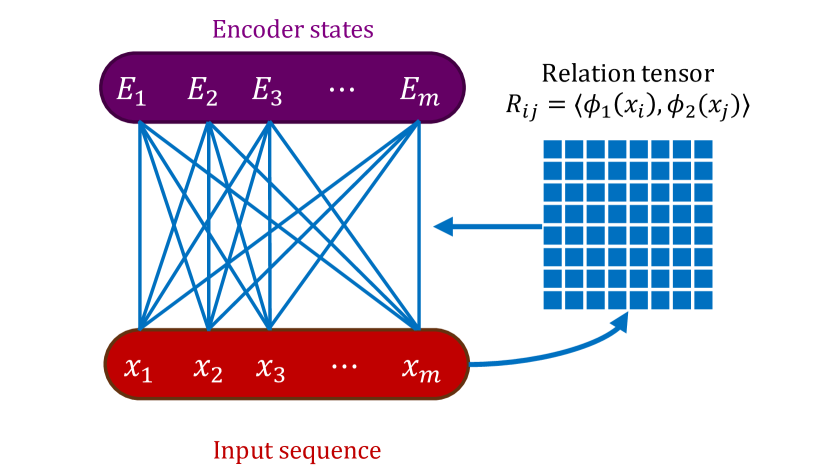
(a) $E\leftarrow\mathrm{SelfAttention}(X)$

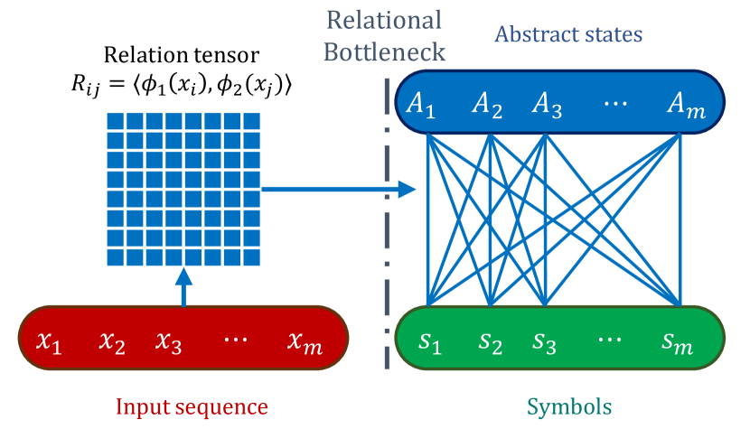
(b) $A\leftarrow\mathrm{RelationalCrossAttention(X,S)}$

Figure 1: Comparison of relational cross-attention with self-attention. Red represents object-level features, blue represents relational features, and purple represents mixed representations. Relational cross-attention computes relational information disentangled from the features of individual objects.

2.3 The Abstractor module

We now describe the Abstractor module. Like the Encoder in a Transformer, this is a module that processes an input sequence of objects $X=\left(x_{1},\ldots,x_{m}\right)$ producing a processed sequence of objects $A=\left(A_{1},\ldots,A_{m}\right)$ that represents features of the input sequence. In an Encoder, the output objects represent a mix of object-level features and relational information. In an Abstractor, the output objects are abstract states that represent purely relational information, abstracted away from the features of individual objects. The core operation in an Abstractor module is relational cross-attention. Mirroring an Encoder, an Abstractor module can comprise several layers, each composed of relational cross-attention followed by a feedforward network. Optionally, residual connections and layer-normalization can be applied as suggested by Vaswani et al., (2017). The algorithmic description is presented in Algorithm 1.

Input : object sequence: $\bm{X}=(x_{1},\ldots,x_{m})\in\mathbb{R}^{d\times m}$

$A^{(0)}\leftarrow S_{1:m}$

for $l\leftarrow 1$ to $L$ do

      

      $A^{(l)}\leftarrow\mathrm{RelationalCrossAttention}\left(X,A^{(l-1)}\right)$

      $A^{(l)}\leftarrow A^{(l)}+A^{(l-1)}$  residual connection (optional)

      $A^{(l)}\leftarrow\mathrm{LayerNorm}(A^{(l)})$  (optional)

      $A^{(l)}\leftarrow\mathrm{FeedForward}\left(A^{(l)}\right)$

end for

Output: $A^{(L)}$

Algorithm 1 Abstractor module

The hyperparameters of an Abstractor module include the number of layers $L$, the relation dimension $d_{r}$ (i.e., number of heads), the projection dimension $d_{p}$ (i.e., key dimension), the relation activation function $\sigma_{\mathrm{rel}}$, and the dimension of the symbols $d_{s}$. The learnable parameters, at each layer, are the projection matrices $W_{1}^{(i)},W_{2}^{(i)}\in\mathbb{R}^{d_{p}\times d_{s}},\ i\in[d_{r}]$, the symbols $S=\left(s_{1},s_{2},\ldots\right)\in\mathbb{R}^{d_{s}\times\texttt{max\_len}}$, and the parameters of the feedforward network. In our experiments, we use a 2-layer feedforward network with a hidden dimension $d_{\mathrm{ff}}$ and ReLU activation. The implementation in the publicly available code includes a few additional hyperparameters including whether to restrict the learned relations to be symmetric (via $W_{1}^{(i)}=W_{2}^{(i)}$), and whether to additionally apply self-attention after relational cross-attention. The symbols in the Abstractor can be either learned parameters or nonparametric positional embeddings (e.g., sinusoidal positional embeddings).

Observe that in the first layer of the Abstractor, the values in relational cross-attention are the input-independent symbols. In the following layers, the values are the abstract states from the previous layer.

Remark (Length generalization).

Similar to positional embeddings in standard Transformers, the symbols $S=(s_{1},s_{2},\ldots)$ can be either learned parameters of the model or non-parametric positional embeddings (e.g., sinusoidal positional embeddings). In principle, using non-parametric positional embeddings as symbols allows for generalization to longer sequence lengths than was observed during training. However, length-generalization remains an unsolved challenge in Transformers (Kazemnejad et al.,, 2023). Although we don’t carry-out a systematic evaluation of length-generalization for Abstractor-based models, it is possible that the same challenges apply. To begin to address this, we propose a variant of the Abstractor which uses position-relative symbols, $S=\left(\ldots,s_{-1},s_{0},s_{1},\ldots\right)$, where the message-passing operation of relational cross-attention becomes

$$A_{i}\leftarrow\mathrm{MessagePassing}\left(\left\{(s_{j-i},R_{ij})\right\}_{j\in[m]}\right)=\sum_{j}R_{ij}s_{j-i}.$$ (7)

Hence, the symbols carry information about relative-position with respect to the object being processed, as opposed to absolute position. In Transformers, relative positional embeddings have been shown to yield improvements in length-generalization. We leave empirical evaluation of this variant to future work.

3 Abstractor architectures

Whereas an Encoder performs “general-purpose” processing, extracting representations of both object-level and relational information, an Abstractor module is more specialized and produces purely relational representations. An Abstractor can be integrated into a broader transformer-based architecture, for enhanced relational processing.

To facilitate the discussion of different architectures, we distinguish between two types of tasks. In a purely relational prediction task, there exists a sufficient statistic of the input which is purely relational and encodes all the information that is relevant for predicting the target. The experiments of (Webb et al.,, 2021; Kerg et al.,, 2022) are examples of discriminative purely relational tasks. An example of a sequence-to-sequence purely relational task is the object-sorting task described in Section 4.2. To predict the ‘argsort’ of a sequence of objects, the pairwise $\prec$ relation is sufficient. Many real-world tasks, however, are not purely relational. In a partially-relational prediction task, the relational information is important, but it is not sufficient for predicting the target. Natural language understanding is an example of a partially-relational task. The math problem-solving experiments in Section 4.3 are also partially-relational.

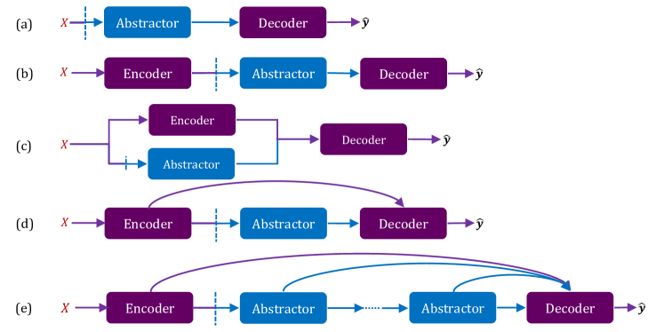
Figure 2: Examples of Abstractor-based model architectures.

The way that an Abstractor module is integrated into a broader model architecture should be informed by the underlying prediction task. Figure 2 depicts several Abstractor architectures each with different properties. Architecture (a) depicts an architecture in which the Abstractor processes the relational features in the input, and the decoder attends to the abstract states $A$. Architecture (b) depicts a model in which the input objects are first processed by an Encoder, followed by an Abstractor for relational processing, and the decoder again attends to the abstract states. These architectures would be appropriate for purely relational tasks since the decoder attends only to the relational representations in the abstract states. Architectures (c) and (d) would be more appropriate for more general tasks which are only partially relational. For example, in architecture (c), the model branches into two parallel processing streams in which an Encoder performs general-purpose processing and an Abstractor performs more specialized processing of relational information. The decoder attends to both the encoder states and abstract states. These architectures use the “multi-attention decoder” described in Algorithm 2 in the appendix. Finally, architecture (e) depicts a composition of Abstractors, wherein the abstract states produced by one Abstractor module are used as input to another Abstractor. This results in computing “higher-order” relational information (i.e., relations on relations). We leave empirical evaluation of this architecture to future work.

4 Experiments

4.1 Discriminative relational tasks

Order relations: modeling asymmetric relations.

A recent related work on relational architectures is (Kerg et al.,, 2022), which identifies and argues for certain inductive biases in relational models. They propose a model called CoRelNet which is, in some sense, the simplest possible model which satisfies those inductive biases. They show that this model is capable of outperforming several previously proposed relational architectures. One inductive bias which they argue for is to model relations between objects as symmetric inner products between object representations. In this section, we aim to add to the discussion on inductive biases for relational learning by arguing that a general relational architecture needs to be able to model asymmetric relations as well.

We generate $N=32$ “random objects” represented by iid Gaussian vectors, $o_{i}\overset{iid}{\sim}\mathcal{N}(0,I_{d})\in\mathbb{R}^{d}$, and associate an order relation to them $o_{1}\prec o_{2}\prec\cdots\prec o_{N}$. Note that $\prec$ is not symmetric. Of the $N^{2}=1024$ possible pairs $(o_{i},o_{j})$, 15% are held out as a validation set (for early stopping) and 35% as a test set. We evaluate learning curves by training on the remaining 50% and computing accuracy on the test set (10 trials for each training set size). Note that the models are evaluated on pairs they have never seen. Thus, the models will need to generalize based on the transitivity of the $\prec$ relation.

We compare three models: an Abstractor, standard (symmetric) CoRelNet, and asymmetric CoRelNet. We observe that standard symmetric CoRelNet is completely unable to learn the task, whereas the Abstractor and asymmetric CoRelNet learn the transitive $\prec$ relation (Figure 4(a)). This can be explained in terms of the relational bottleneck. In a relational task, there exists a sufficient statistic which is relational. The relational bottleneck restricts the search space of representations to be a space of relational features, making the search for a good representation more sample efficient. In a task in which there exists a sufficient statistic involving a symmetric relation (as is the case with the same/different tasks considered in (Kerg et al.,, 2022)), we can further restrict the search space to symmetric relational representations, making learning a good representation even more sample efficient. However, some relations are more complex and may be asymmetric—an example is order relations. Symmetric inner products don’t have the representational capacity to model such relations. But asymmetric inner products with different learned left and right encoders can model such relations.

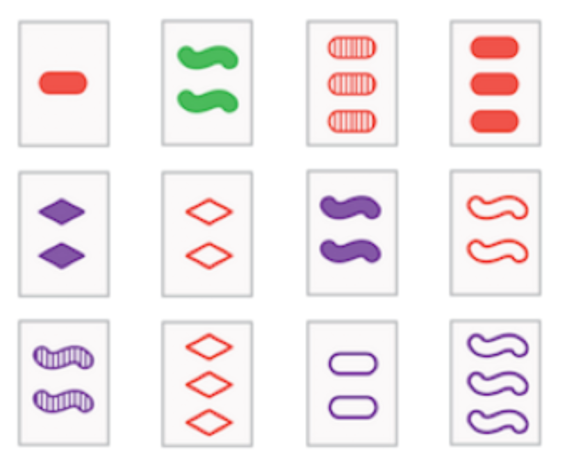
Figure 3: The SET game

SET: modeling multi-dimensional relations.

“SET” is a cognitive task in which players are presented with a sequence of cards, each of which contains figures that vary along four dimensions (color, number, pattern, and shape) and they must find triplets of cards which obey a deceptively simple rule: along each dimension, cards in a ‘SET’ must either have the same value or three unique values. In this experiment, the task is: given a triplet of card images, determine whether they form a SET or not.

We compare an Abstractor model to CoRelNet. The shared architecture is $\texttt{CNN}\to\{\texttt{Abstractor}\text{ or }\texttt{CorelNet}\}\to\texttt{Flatten}\to\texttt{Dense}$. The CNN embedder is obtained through a pre-training task. We report learning curves in Figure 4(b) (10 trials per training set size). We find that the Abstractor model significantly out-performs CoRelNet. We attribute this to its ability to model multi-dimensional relations. In this task, there exists four different relations (one for each attribute) which are needed to determine whether a triple of cards forms a set. CoRelNet would need to squeeze all of this information into a single-dimensional scalar whereas the Abstractor can model each relation separately. We hypothesize that the ability to model relations as multi-dimensional is also the reason that the Abstractor can learn the order relation better than asymmetric CoRelNet—even though the underlying relation is “one-dimensional”, having a multi-dimensional representation enables greater robustness and multiple avenues towards a good solution during optimization.

SET (continued): comparison to “symbolic” relations.

In Figure 4(c), to evaluate the relational representations produced by Abstractors, we compare an Abstractor-based model to a “symbolic” model which receives as input a binary representation of the four relevant relations. We train 1-head Abstractors separately for each of the four attributes to learn same/different relations, where the task is to decide if an input pair of cards is the same or different for that attribute. We then use the learned $W_{1}$ and $W_{2}$ parameters learned for these relations to initialize the relations in a multi-head Abstractor. The Abstractor is then trained on a dataset of triples of cards, half of which form a SET.

This is compared to a baseline symbolic model where, instead of images, the input is a vector with 12 bits, explicitly encoding the relations. That is, for each of the four attributes, a binary symbol is computed for each pair of three input cards—1 if the pair is the same in that attribute, and 0 otherwise. A two-layer MLP is then trained to decide if the triple forms a SET. The MLP using the symbolic representation represents an upper bound on the performance achievable by any model. This comparison shows that the relational representations produced by an Abstractor result in a sample efficiency that is not far from that obtained with purely symbolic encodings of the relevant relations.

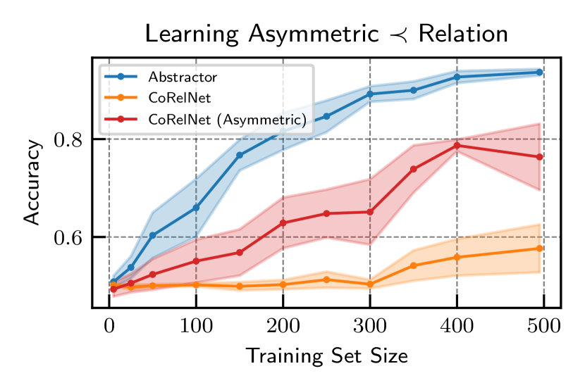
(a) The $\prec$ relation can be learned with asymmetric but not symmetric inner products.

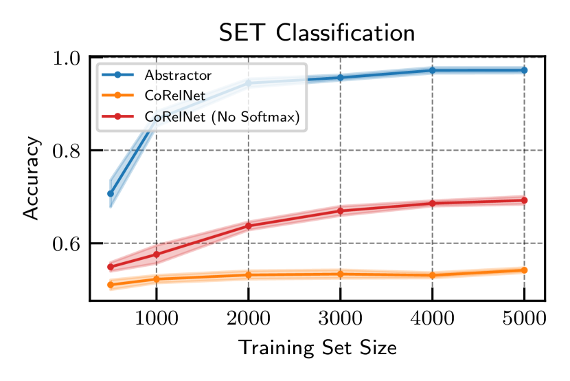
(b) The Abstractor’s ability to model multi-dimensional relations enables it to solve SET.

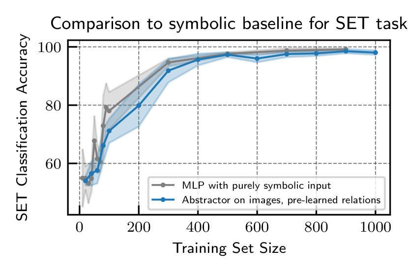
(c) Comparison of Abstractor trained on card images and MLP with hand-encoded relations.

Figure 4: Experiments on discriminative relational tasks and comparison to CoRelNet.

4.2 Object-sorting: purely relational sequence-to-sequence tasks

In the following set of experiments, we consider sequence-to-sequence tasks which are purely relational, and compare an Abstractor-supported model to a standard Transformer. We consider the task of sorting sequences of random objects. This task is “purely relational” in the sense that there exists a relation (order) which is a sufficient statistic for solving the task—the features of individual objects beyond this relation are extraneous. This is a more controlled setting which tests the hypothesis that the inductive biases of the Abstractor confer benefits in modeling relations. The experiments in the present section demonstrate that the Abstractor enables a dramatic improvement in sample-efficiency on sequence-to-sequence relational tasks.

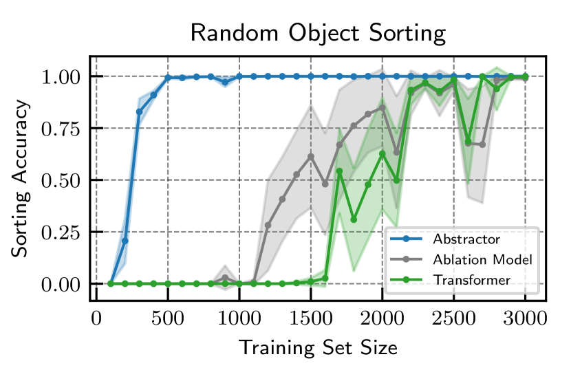
(a) Learning curves on sorting sequences of random objects. The abstractor is dramatically more sample-efficient.

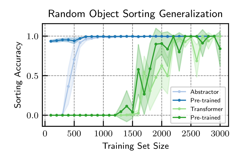
(b) Learning curves with and without pre-training on a similar sorting task. The Abstractor benefits from pre-training.

Figure 5: Experiments on object-sorting, a purely relational sequence-to-sequence tasks.

Superior sample-efficiency on relational seq2seq tasks.

We generate random objects in the following way. First, we generate two sets of random attributes $\mathcal{A}=\{a_{1},a_{2},a_{3},a_{4}\}$, $a_{i}\overset{iid}{\sim}\mathcal{N}(0,I)\in\mathbb{R}^{4}$ and $\mathcal{B}=\{b_{1},\ldots,b_{12}\}$, $b_{i}\overset{iid}{\sim}\mathcal{N}(0,I)\in\mathbb{R}^{8}$. To each set of attributes, we associate the strict ordering relation $a_{1}\prec a_{2}\prec a_{3}\prec a_{4}$ and $b_{1}\prec b_{2}\prec\cdots\prec b_{12}$, respectively. Our random objects are formed by the Cartesian product of these two attributes $\mathcal{O}=\mathcal{A}\times\mathcal{B}$, yielding $N=4\times 12=48$ objects. Then, we associate with $\mathcal{O}$ the strict ordering relation corresponding to the order relation of $\mathcal{A}$ as the primary key and the order relation of $\mathcal{B}$ as the secondary key. I.e., $(a_{i},b_{j})\prec(a_{k},b_{l})$ if $a_{i}\prec a_{k}$ or if $a_{i}=a_{k}$ and $b_{j}\prec b_{l}$.

Given a set of objects in $\mathcal{O}$, the task is to sort it according to $\prec$. The input sequences are randomly permuted sequences of $10$ objects in $\mathcal{O}$ and the target sequences are the indices of the object sequences in sorted order (i.e., ‘argsort’). The training data are sampled uniformly from the set of length-10 sequences in $\mathcal{O}$. We also generate non-overlapping validation and testing datasets.

We evaluate learning curves on an Abstractor, a standard Transformer, and an “Ablation” model (10 trials for each training set size). The Abstractor uses the architecture $\texttt{Encoder}\to\texttt{Abstractor}\to\texttt{Decoder}$ (architecture (b) in Figure 2). The Encoder-to-Abstractor interface uses relational cross-attention and the Abstractor-to-Decoder interface uses standard cross-attention. The Ablation Model aims to test the effects of the relational cross-attention in the Abstractor model—it is architecturally identical to the Abstractor model with the crucial exception that the Encoder-to-Abstractor interface instead uses standard cross-attention. The hyperparameters of the models are chosen so that the parameter counts are similar (details in Appendix B). We find that the Abstractor is dramatically more sample-efficient than the Transformer and the Ablation model (Figure 5(a)).

Ability to generalize to similar tasks.

We also used the object-sorting task and the dataset generated as described above to test the Abstractor’s ability to generalize from similar relational tasks through pre-training. The main task uses the same dataset described above. The pre-training task involves the same object set $\mathcal{O}$ but with a modified order relation. The ordering in attribute $\mathcal{A}$ is randomly permuted, while the ordering in attribute $\mathcal{B}$ is kept the same.

The Abstractor model here uses architecture (a) in Figure 2 (i.e., no Encoder), and the transformer is the same as the previous section. We pre-train both models on the pre-training task and then, using those learned weights for initialization, evaluate learning curves on the original task. Since the Transformer requires more training samples to learn the object-sorting task, we use a pre-training set size of $3,000$, chosen to be large enough for the Transformer to learn the pre-training task. This experiment assesses the models’ ability to generalize relations learned on one task to a new task. Figure 5(b) shows the learning curves for each model with and without pre-training. We observe that when the Abstractor is pre-trained, its learning curve on the object-sorting task is significantly accelerated, whereas the transformer does not benefit from pre-training.

4.3 Math problem-solving: partially-relational sequence-to-sequence tasks

The object-sorting experiments in the previous section are “purely relational” in the sense that the set of pairwise $\prec$ relations is a sufficient statistic for solving the task. In a general sequence-to-sequence task, there may not be a relation which is a sufficient statistic. Nonetheless, relational reasoning may still be crucial for solving the task, and the enhanced relational reasoning capabilities of the Abstractor may enable performance improvements. The “partially-relational” architectures described in Section 3 enable a branch of the model to focus on relational reasoning while maintaining a connection to object-level attributes. In this section, we evaluate an Abstractor model using architecture (d) of Figure 2 on a set of math problem-solving tasks based on the dataset proposed in (Saxton et al.,, 2019).

Task: polynomials__expand Question: Expand (2*x + 3)*(x - 1). Answer: 2*x**2 + x - 3

Task: algebra__linear_1d Question: Solve for z: 5*z + 2 = 9. Answer: 7/5

Figure 6: Examples of input/target sequences from the math problem-solving dataset.

The dataset consists of several math problem-solving tasks, with each task having a dataset of question-answer pairs. The tasks include solving equations, expanding products of polynomials, differentiating functions, predicting the next term in a sequence, etc. A sample of question-answer pairs is displayed in Figure 6. The overall dataset contains $2\times 10^{6}$ training examples and $10^{4}$ validation examples per task. Questions have a maximum length of 160 characters and answers have a maximum length of 30 characters. We use character-level encoding with a common alphabet of size $95$ (including upper/lower case characters, digits, and punctuation). Each question and answer is tokenized and padded with the null character.

We compare an Abstractor model using architecture (d) in Figure 2 to a standard Transformer. Since the Abstractor-based model with architecture (d) has an Abstractor module in addition to an Encoder and Decoder, we compare against two versions of the Transformer in order to control for parameter count. In the first, the Encoder/Decoder have identical hyperparameters to the Abstractor model. In the second, we increase the model dimension and hidden layer size of the feedforward network such that the overall parameter count is approximately the same as the Abstractor model. We refer to the first model as “Transformer” and the second as “Transformer+” in the figures. We train on modestly sized models. The precise architectural details and hyperparameters are described in Appendix B.

We evaluate the three models on 5 tasks within the dataset: differentiating functions (calculus); predicting the next term in a sequence (algebra); solving a linear equation (algebra); expanding polynomials; and adding polynomials. For each, we train on the training split and track the teacher-forcing accuracy (excluding null characters) on the validation split. For each pair of model and task, we repeat the experiment 5 times and report error bars as twice the standard error of mean.

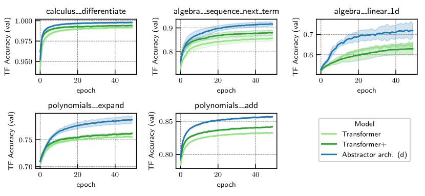
Figure 7: Training curves comparing an Abstractor-based architecture to a standard Transformer on mathematics problem-solving tasks.

Figure 7 shows the validation teacher-forcing accuracy during the course of training. We observe a modest improvement in accuracy compared to both ‘Transformer’ and ‘Transformer+’ across all tasks. The larger Transformer tends to perform better than the smaller Transformer, but the Abstractor-based model consistently outperforms both. This indicates that the performance improvement stems from the architectural modification rather than merely the increase in parameter count. We conjecture that a “partially-relational” Abstractor architecture (e.g., architecture (d)) implements two branches of information-processing. The Encoder performs more general-purpose processing of the input sequence, while the Abstractor performs more specialized relational processing. The Decoder then has access to both representations, enabling it to perform the task more effectively.

5 Discussion

In this work, we propose a variant of attention that produces representations of relational information disentangled from object-level attributes. This leads to the development of the Abstractor module, which fits naturally into the powerful framework of Transformers. Through a series of experiments, we demonstrate the potential of this new framework to achieve gains in sample efficiency in both purely relational tasks and more general sequence modeling tasks.

This work opens up several avenues for future research. One possible line of research is to better understand the role of symbols within the Abstractor, including the trade-offs between learned symbols, parametric symbols, and the use of position-relative symbols. Another important line of research is the study of the alternative architectural variants proposed in Figure 2. For example, understanding the properties of compositions of Abstractor modules and assessing such an architecture’s ability to represent higher-order relations will shed light on the expressive power of the framework. Finally, the experiments presented here demonstrate the Abstractor’s promise and utility for relational representation in Transformers, and it will be interesting to explore the framework’s use in increasingly complex modeling problems.

Code and Data

Code, experimental logs, and instructions for reproducing our results are available at: https://github.com/Awni00/abstractor

Appendix A Multi-Attention Decoder

Input :  Target sequence: $\bm{y}=(y_{0},\ldots,y_{l_{y}-1})$,

Context sequences: $X^{(i)}=(x_{1}^{(i)},\ldots,x_{l_{i}}^{(i)}),\ i=1,\ldots,K$

$D^{(0)}\leftarrow\bm{y}$

for $l\leftarrow 1$ to $L$ do

      

      $D^{(l)}\leftarrow\mathrm{CausalSelfAttention}\left(D^{(l-1)}\right)$

      residual connection and layer-normalization

      for $i\leftarrow 1$ to $K$ do

             $D^{(l)}\leftarrow\mathrm{CrossAttention}\left(D^{(l)},X^{(i)}\right)$

            residual connection and layer-normalization

       end for

      

      $D^{(l)}\leftarrow\mathrm{FeedForward}\left(D^{(l)}\right)$

end for

Output: $D^{(L)}$

Algorithm 2 Multi-Attention Decoder

Appendix B Experimental details

In this section, we give further experimental details including architectures, hyperparameters, and implementation details. All model and experiments are implemented in Tensorflow. The code is publicly available on the project repo along with detailed experimental logs and instructions for reproduction. We implement all models “from scratch” in Tensorflow, using only built-in implementations of basic layers.

B.1 Discriminative tasks (Section 4.1)

B.1.1 Pairwise Order

Abstractor architecture number of layers $L=1$, relation dimension $d_{r}=4$, symbol dimension $d_{s}=64$, projection dimension $d_{p}=16$, feedforward hidden dimension $d_{\mathrm{ff}}=64$, relation activation function $\sigma_{\mathrm{rel}}=\mathrm{sigmoid}$. No layer normalization or residual connection. The symbols are learned parameters.

CoRelNet Architecture Given a sequence of objects, $X=(x_{1},\ldots,x_{m})$, standard CoRelNet simply computes the inner product and takes the Softmax. We also add a learnable linear map, $W\in\mathbb{R}^{d\times d}$. Hence, $R=\text{Softmax}(A),A={\left[\langle Wx_{i},Wx_{j}\rangle\right]}_{ij}$. The asymmetric variant of CoRelNet is given by $R=\text{Softmax}(A),A={\left[\langle W_{1}x_{i},W_{2}x_{j}\rangle\right]}_{ij}$, where $W_{1},W_{2}\in\mathbb{R}^{d\times d}$ are learnable matrices.

Training/Evaluation We use the sparse categorical crossentropy loss and the Adam optimizer with a learning rate of $10^{-2}$, $\beta_{1}=0.9,\beta_{2}=0.999,\varepsilon=10^{-7}$. We use a batch size of 64. We train for 100 epochs and restore the best model according to validation loss. We evaluate on the test set.

B.1.2 SET

The card images are RGB images of dimension $70\times 50$. The CNN embedder produces embeddings fo dimension $d=64$ for each card. The CNN is trained to predict the four attributes of each card and then an embedding for each card is obtained from an intermediate layer (i.e., the parameters of the CNN are then frozen). Recall that the common architecture is $\texttt{CNN Embedder}\to\{\texttt{Abstractor}\text{ or }\texttt{CoRelNet}\}\to\texttt{Flatten}\to\texttt{Dense(2)}$. We tested against the standard version of CorelNet, but found that it did not learn anything. We iterated over the hyperparameters and architecture to improve its performance. We found that removing the softmax activation in CoRelNet improved performance a bit. We describe hyperparameters below.

Common embedder’s architecture The architecture is given by Conv2D $\to$ MaxPool2D $\to$ Conv2D $\to$ MaxPool2D $\to$ Flatten $\to$ Dense(64, ’relu’) $\to$ Dense(64, ’relu’) $\to$ Dense(2). The embedding is extracted from the penultimate layer. The CNN is trained to predict the four attributes of each card until it reaches perfect accuracy and near-zero loss.

Abstractor architecture The Abstractor module has hyperparameters: number of layers $L=1$, relation dimension $d_{r}=4$, symmetric relations (i.e., $W_{1}^{(i)}=W_{2}^{(i)}$, $i\in[d_{r}]$), linear relation activation (i.e., $\sigma_{\mathrm{rel}}:x\mapsto x$), symbol dimension $d_{s}=64$, projection dimension $d_{p}=16$, feedforward hidden dimension $d_{\mathrm{ff}}=128$, and no layer normalization or residual connection. The symbols are learned parameters.

CoRelNet Architecture Standard CoRelNet is described above. It simply computes, $R=\text{Softmax}(A),A={\left[\langle Wx_{i},Wx_{j}\rangle\right]}_{ij}$. This variant was stuck at 50% accuracy regardless of training set size. We found that removing the Softmax helped. Figure 4(b) compares against both variants of CoRelNet.

This finding suggests that allowing $\sigma_{\mathrm{rel}}$ to be a configurable hyperparameter is a useful feature of the Abstractor. Softmax performs contextual normalization of relations, such that the relation between $i$ and $j$ is normalized in terms of $i$’s relations with all other objects. This may be useful at times, but may also cripple a relational model when it is more useful to represent an absolute relation between a pair of objects, independently of the relations with other objects.

Data generation The data is generated by randomly sampling a SET with probability 1/2 and a non-SET with probability 1/2. The triplet of cards is then randomly shuffled.

Training/Evaluation We use the sparse categorical crossentropy loss and the Adam optimizer with a learning rate of $10^{-3}$, $\beta_{1}=0.9,\beta_{2}=0.999,\varepsilon=10^{-7}$. We use a batch size of 64. We train for 200 epochs and restore the best model according to validation loss. We evaluate on the test set.

B.2 Relational sequence-to-sequence tasks (Section 4.2)

B.2.1 Sample-efficiency in relational seq2seq tasks

Abstractor architecture The Abstractor model uses architecture (b) of Figure 2. For each of the Encoder, Abstractor, and Decoder modules, we use 2 layers, 2 attention heads/relation dimensions, a feedforward network with 64 units and an embedding/symbol dimension of 64. The Abstractor’s symbols are learned parameters of the model, and uses $\sigma_{\mathrm{rel}}=\mathrm{Softmax}$. The number of trainable parameters is $386,954$.

Transformer architecture We implement the standard Transformer of (Vaswani et al.,, 2017). For both the Encoder and Decoder modules, we use 4 layers, 2 attention heads, a feedforward network with 64 units and an embedding dimension of 64. The number of trainable parameters is $469,898$. We increased the number of layers compared to the Abstractor in order to make it a comparable size in terms of parameter count. Previously, we experimented with identical hyperparameters (where the Transformer would have fewer parameters due to not having an Abstractor module).

Ablation model architecture The Ablation model uses an identical architecture to the Abstractor, except that the relational cross-attention is replaced with standard cross attention at the Encoder-Abstractor interface (with $Q\leftarrow A,K\leftarrow E,V\leftarrow E$). It has the same number of parameters as the Abstractor-based model.

Training/Evaluation We use the sparse categorical crossentropy loss and the Adam optimizer with a learning rate of $10^{-3}$, $\beta_{1}=0.9,\beta_{2}=0.999,\varepsilon=10^{-7}$. We use a batch size of 512. We train for 100 epochs and restore the best model according to validation loss. We evaluate learning curves by varying the training set size and sampling a random subset of the data at that size. Learning curves are evaluated starting at 100 samples up to 3000 samples in increments of 100 samples. We repeat each experiment 10 times and report the mean and standard error of the mean.

B.2.2 Generalization to new object-sorting tasks

Abstractor architecture The Abstractor model uses architecture (a) of Figure 2. The Abstractor module has 1 layer, a symbol dimension of 64, a relation dimension of 4, a softmax relation activation, and a 64-unit feedforward network. The decoder also has 1 layer with 4-head MHA and a 64-unit feedforward network.

Transformer architecture The Transformer is identical to the previous section.

Training/Evaluation The loss, optimizer, batch size, and learning curve evaluation steps are identical to the previous sections. Two object-sorting datasets are created based on an “attribute-product structure”—an primary dataset and a pre-training dataset. As described in Section 4.2, the pre-training dataset uses the same random objects as the primary dataset but with the order relation of the primary attribute reshuffled. The models are trained on 3,000 labeled sequences of the pre-training task and the weights are used to initialize training on the primary task. Learning curves are evaluated with and without pre-training for each model.

B.3 Math Problem-Solving (Section 4.3)

Abstractor architecture The Abstractor model uses architecture (d) of Figure 2. The Encoder, ABstractor, and Decoder modules share the same hyperparameters: number of layers $L=1$, relation dimension/number of heads $d_{r}=n_{h}=4$, symbol dimension/model dimension $d_{s}=d_{\mathrm{model}}=128$, projection dimension $d_{p}=32$, feedforward hidden dimension $d_{\mathrm{ff}}=256$. In the Abstractor, the relation activation function is $\sigma_{\mathrm{rel}}=\mathrm{softmax}$, and the symbols are nonparametric sinusoidal positional embeddings.

Transformer architecture The Transformer Encoder and Decoder have identical hyperparameters to the Encoder and Decoder of the Abstractor architecture.

Transformer+ architecture In ‘Transformer+’, the model dimension is increased $d_{\mathrm{model}}=200$ and the feedforward hidden dimension are increased to $d_{\mathrm{ff}}=400$. The remaining hyperparameters are the same.

Training/Evaluation We train each model for 50 epochs with the categorical cross-entropy loss and the Adam optimizer using a learning rate of $6\times 10^{-4}$, $\beta_{1}=0.9,\beta_{2}=0.995,\varepsilon=10^{-9}$. We use a batch size of 128.

Appendix C Additional Experiments

C.1 Object-sorting: Robustness and Out-of-Distribution generalization

This experiment explores the Abstractor’s robustness to noise and out-of-distribution generalization as compared to a standard Transformer. We consider the models in Section 4.2 and the corresponding object-sorting task. We train each model on this task using 3,000 labeled sequences. We choose the fixed training set size of 3,000 because is large enough that both the Abstractor and Transformer are able to learn the task. Then, we corrupt the objects with noise and evaluate performance on sequences in the hold-out test set where objects are replaced by their corrupted versions. We evaluate robustness to a random linear map as well as to additive noise, while varying the noise level. We evaluate over several trials, averaging over the realizations of the random noise.

On the hold out test set, we corrupt the object representations by applying a random linear transformation. In particular, we randomly sample a random matrix the entries of which are iid zero-mean Gaussian with variance $\sigma^{2}$, $\Phi\in\mathbb{R}^{d\times d},\Phi_{ij}\sim\mathcal{N}(0,\sigma^{2})$. Each object in $\mathcal{O}$ is then corrupted by this random linear transformation, $\widetilde{o}_{i}=\Phi o_{i},\ \text{ for each }i\in[48]$. We also test robustness to additive noise via $\widetilde{o}_{i}=o_{i}+\varepsilon_{i},\varepsilon_{i}\sim\mathcal{N}(0,\sigma^{2}I_{d})$.

The models are evaluated on the hold-out test set with objects replaced by their corrupted version. We evaluate the sorting accuracy of each model while varying the noise level $\sigma$ (5 trials at each noise level). The results are shown in figures 8(a) and 8(b). We emphasize that the models are trained only on the original objects in $\mathcal{O}$, and are not trained on objects corrupted by any kind of noise.

This experiment can be interpreted in two lights: the first is robustness to noise. The second is a form of out-of-distribution generalization. Note that the objects seen by the models post-corruption lie in a different space than those seen during training. Hence the models need to learn relations that are in some sense independent of the value representation. As a theoretical justification for this behavior, Zhou et al., (2009) shows that $\langle\Phi x,\Phi y\rangle\approx\langle x,y\rangle$ in high dimensions, for a random matrix $\Phi$ with iid Gaussian entries. This indicates that models whose primary computations are performed via inner products, like Abstractors, may be more robust to this kind of corruption.

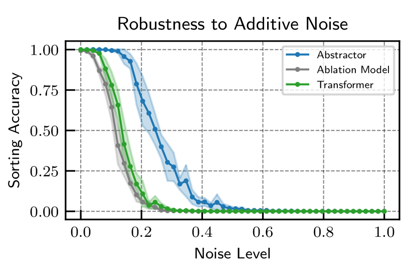
(a) The Abstractor is more robust to corruption by additive noise.

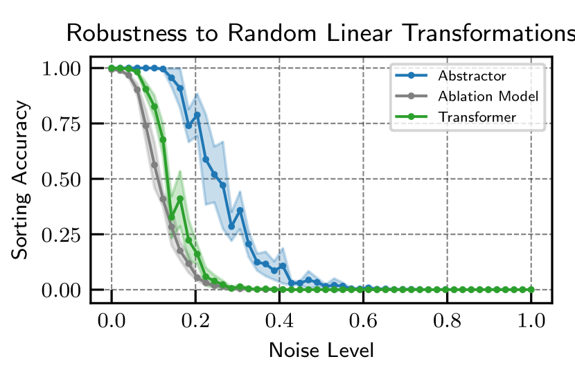
(b) The Abstractor is more robust to corruption by a random linear transformation.

Figure 8: Experiments on robustness.

References

- Barrett et al., (2018) Barrett, D. G., Hill, F., Santoro, A., Morcos, A. S., and Lillicrap, T. (2018). Measuring abstract reasoning in neural networks. In Proceedings ICML.
- Battaglia et al., (2018) Battaglia, P. W., Hamrick, J. B., Bapst, V., Sanchez-Gonzalez, A., Zambaldi, V., Malinowski, M., Tacchetti, A., Raposo, D., Santoro, A., Faulkner, R., Gulcehre, C., Song, F., Ballard, A., Gilmer, J., Dahl, G., Vaswani, A., Allen, K., Nash, C., Langston, V., Dyer, C., Heess, N., Wierstra, D., Kohli, P., Botvinick, M., Vinyals, O., Li, Y., and Pascanu, R. (2018). Relational inductive biases, deep learning, and graph networks. arXiv:1806.01261.
- Graves et al., (2014) Graves, A., Wayne, G., and Danihelka, I. (2014). Neural Turing machines. arXiv:1410.5401.
- Holyoak, (2012) Holyoak, K. J. (2012). Analogy and relational reasoning. In Holyoak, K. J. and Morrison, R. G., editors, The Oxford Handbook of Thinking and Reasoning. New York: Oxford University Press.
- Kazemnejad et al., (2023) Kazemnejad, A., Padhi, I., Ramamurthy, K. N., Das, P., and Reddy, S. (2023). The Impact of Positional Encoding on Length Generalization in Transformers.
- Kerg et al., (2020) Kerg, G., Kanuparthi, B., Goyal, A., Goyette, K., Bengio, Y., and Lajoie, G. (2020). Untangling tradeoffs between recurrence and self-attention in artificial neural networks. Advances in Neural Information Processing Systems, 33:19443–19454.
- Kerg et al., (2022) Kerg, G., Mittal, S., Rolnick, D., Bengio, Y., Richards, B., and Lajoie, G. (2022). On neural architecture inductive biases for relational tasks. arXiv preprint arXiv:2206.05056.
- Mahowald et al., (2023) Mahowald, K., Ivanova, A. A., Blank, I. A., Kanwisher, N., Tenenbaum, J. B., and Fedorenko, E. (2023). Dissociating language and thought in large language models: A cognitive perspective. arXiv preprint arXiv:2301.06627.
- Mondal et al., (2023) Mondal, S. S., Webb, T. W., and Cohen, J. (2023). Learning to reason over visual objects. In International Conference on Learning Representations.
- Pritzel et al., (2017) Pritzel, A., Uria, B., Srinivasan, S., Badia, A. P., Vinyals, O., Hassabis, D., Wierstra, D., and Blundell, C. (2017). Neural episodic control. In International conference on machine learning, pages 2827–2836. PMLR.
- Santoro et al., (2017) Santoro, A., Raposo, D., Barrett, D. G., Malinowski, M., Pascanu, R., Battaglia, P., and Lillicrap, T. (2017). A simple neural network module for relational reasoning. In Advances in neural information processing systems, pages 4967–4976.
- Saxton et al., (2019) Saxton, D., Kohli, P., Grefenstette, E., and Hill, F. (2019). Analyzing Mathematical Reasoning Abilities of Neural Models.
- Shanahan et al., (2020) Shanahan, M., Nikiforou, K., Creswell, A., Kaplanis, C., Barrett, D., and Garnelo, M. (2020). An explicitly relational neural network architecture. In III, H. D. and Singh, A., editors, Proceedings of the 37th International Conference on Machine Learning, volume 119 of Proceedings of Machine Learning Research, pages 8593–8603. PMLR.
- Snow et al., (1984) Snow, R. E., Kyllonen, P. C., and Marshalek, B. (1984). The topography of ability and learning correlations. In Sternberg, R. J., editor, Advances in the psychology of human intelligence, volume 2, pages 47–103.
- Vaswani et al., (2017) Vaswani, A., Shazeer, N., Parmar, N., Uszkoreit, J., Jones, L., Gomez, A. N., Kaiser, Ł., and Polosukhin, I. (2017). Attention is all you need. Advances in neural information processing systems, 30.
- Webb et al., (2022) Webb, T., Holyoak, K. J., and Lu, H. (2022). Emergent analogical reasoning in large language models. arXiv:2212.09196.
- Webb et al., (2021) Webb, T., Sinha, I., and Cohen, J. D. (2021). Emergent symbols through binding in external memory. In 9th International Conference on Learning Representations, ICLR 2021, Virtual Event, Austria, May 3-7, 2021. OpenReview.net.
- Webb et al., (2023) Webb, T. W., Frankland, S. M., Altabaa, A., Krishnamurthy, K., Campbell, D., Russin, J., O’Reilly, R., Lafferty, J., and Cohen, J. D. (2023). The relational bottleneck as an inductive bias for efficient abstraction. arXiv:2309.06629.
- Whittington et al., (2020) Whittington, J. C., Muller, T. H., Mark, S., Chen, G., Barry, C., Burgess, N., and Behrens, T. E. (2020). The Tolman-Eichenbaum machine: Unifying space and relational memory through generalization in the hippocampal formation. Cell, 183(5):1249–1263.e23.
- Wolf et al., (2020) Wolf, T., Debut, L., Sanh, V., Chaumond, J., Delangue, C., Moi, A., Cistac, P., Rault, T., Louf, R., Funtowicz, M., et al. (2020). Transformers: State-of-the-art natural language processing. In Proceedings of the 2020 conference on empirical methods in natural language processing: system demonstrations, pages 38–45.
- Zhou et al., (2009) Zhou, S., Lafferty, J., and Wasserman, L. (2009). Compressed and privacy-sensitive sparse regression. IEEE Trans. Information Theory, 55(2):846–866.