Force-coordination Control for Aerial Collaborative Transportation based on Lumped Disturbance Separation and Estimation

Abstract

This article studies the collaborative transportation of a cable-suspended pipe by two quadrotors. A force-coordination control scheme is proposed, where a force-consensus term is introduced to average the load distribution between the quadrotors. Since thrust uncertainty and cable force are coupled together in the acceleration channel, disturbance observer can only obtain the lumped disturbance estimate. Under the quasi-static condition, a disturbance separation strategy is developed to remove the thrust uncertainty estimate for precise cable force estimation. The stability of the overall system is analyzed using Lyapunov theory. Both numerical simulations and indoor experiments using heterogeneous quadrotors validate the effectiveness of thrust uncertainty separation and force-consensus algorithm.

I Introduction

Recent years have witnessed increasing application in the area of drone delivery. The bottleneck problem of aerial transportation lies in the limitation of the payload capacity. Although using a larger vehicle may solve this problem, it is believed to be more costly and inefficient. As described in [1], when the size of a rotorcraft increases to a certain point, the growth in relative productivity becomes trivial.

Multi-UAV collaboration is a potentially promising choice to increase the transportation capacity. On top of this, additional task redundancy, lower cost, and robustness to vehicle failure may also be provided [2, 3, 4, 5]. Generally, the UAV-payload connection types include active connections and passive connections [6]. Active connection involves equipping the vehicle with a gripper to grasp and hold the payload rigidly [7], while passive connection refers to suspending the payload through cables [8] or via a universal joint [9]. The gripper attachment increases the mass and inertia of the system considerably and thereby makes the system respond slowly. In contrast, the cable suspension mechanism is more appealing for its low cost and flexible system structure. Therefore, we adopt the cable suspension mechanism for collaborative transportation in this research.

The state of the art of control strategies for cable-suspended collaborative transportation can be divided into two groups [10]: payload-based design and formation-based design. Payload-based design focuses on the trajectory of the payload, e.g., [11, 12, 13]. Although the precise attitude and position control of the payload can be realized, the dynamic information of the payload is required for real-time feedback control, which is hard to obtain in engineering practice. In contrast, in formation-based design, only the state information of the aerial vehicles is needed. When the vehicle group reaches its destination, the payload is also supposed to reach the target area. The validity and feasibility of such approach has been established via simulation [14] and experiment [15], but the cable forces on the quadrotors are ignored.

To implement formation-based robust collaborative transportation, several control algorithms have been developed. A distanced-based formation control algorithm for a team of quadrotors transporting a heavy object is presented in [16], which measures and resists the acceleration due to disturbances and rope tension using incremental nonlinear dynamic inversion control. In [17] and [18], a passivity-based formation control strategy is proposed with adaptive compensation terms to eliminate the wind disturbance and the cable tension. The energy passivity property of the quadrotors-payload system is established in [19], where an adaptive damping term is used to dissipate the energy injected by the sudden perturbations.

The studies mentioned above are all designed based on the rigid formation. As a matter of fact, maintaining a fixed formation for payload transportation is not necessary and it is better to employ a flexible formation, which can adapt the vehicles to the complex and uncertain environment and tasks [20]. Force control-based approaches have been explored for collaborative payload transportation with flexible formation, e.g., force amplification [21] and contact force regulation [22]. The so-called Force-Amplifying N-Robot Transport System (Force-ANTS) control framework is introduced in [21] to achieve force-coordination among a group of ground robots. The follower robots perceive the leader force by simply measuring the object’s motion locally and then reinforce this intention, which makes it possible to cooperatively transport heavy objects of various sizes without any communication network. In [22], a new adaptive force-consensus algorithm is proposed to guarantee the average load distribution among the vehicles using force/acceleration sensors. This work can average the energy consumption among the UAVs and thereby extend the endurance of the entire team. Cooperative manipulation of a cable-suspended payload with two aerial vehicles is considered in [23], where the role of the internal force is first studied and analyzed in depth. Although simulation results have verified the effectiveness of the methods in [22] and [23], these methods cannot be applied directly in practice because model uncertainties are not considered.

In this article, we propose a force-coordination control strategy for cable-suspended collaborative transportation. Here the concept of force-coordination means that cable forces between the payload and aerial vehicles converge to the expected values cooperatively, which is believed to play a fundamental role in more difficult aerial cooperative payload manipulations, such as swinging a payload [24]. The most critical step for applying force-coordination-based control is the accurate measurement of contact force. In [25] and [26], force sensors are installed to measure the cable tensions. However, in addition to the high cost, the force sensor complicates the vehicle’s structure and increases the weight of the whole system, whereas force estimation is more appropriate for its low cost and convenience. The existing external force estimation methods, e.g., disturbance observer (DO) [27], extended state observer (ESO) [28], and unscented Kalman filter (UKF) [29], can only estimate the equivalent lumped disturbance rather than distinguish different disturbances in the same channel. The cable tension is always coupled with multiple disturbances, like thrust uncertainty, wind force, and mass center offset, in the acceleration channel. Therefore, it is not a straightforward task to estimate the cable force precisely. An attempt is made to estimate the contact force of rigidly connected payload for admittance control in [9]. To avoid the undesirable offset in the estimated force caused by wind and model uncertainties, a Finite State Machine is employed to monitor the magnitude of the force and decides whether to reject or utilize the estimate for trajectory generation. This strategy seems quite fascinating and practical for its robustness to disturbances, but essentially it only evaluates the quality of estimation and does not improve the force estimation accuracy.

This paper studies the collaborative transportation system composed of two aerial vehicles carrying a cable-suspended long pipe. The lengths of the cables are different and unknown, so that we can treat this system as a heterogeneous coordination system. For quadrotor dynamics, among the multiple disturbances mixed with the cable force, thrust uncertainty is the primary one, which is the synthesis of uncertainties in the whole propulsion system. Uncertainties in the propulsion system include aerodynamic uncertainties and hardware uncertainties. Here aerodynamic uncertainties refer to the thrust coefficients, which are consistent for the same blades. However, hardware uncertainties vary from one-to-one, including motor degradation, blade damage, battery wear, electronic speed controller efficiency loss, and so on. Therefore, to acquire an accurate cable force estimate, it is necessary to get rid of the thrust uncertainty. The main contributions are summarized in the following aspects:

1. A force-coordination control scheme is proposed for the collaborative transportation system. Different from the position-coordination control methods [17, 18, 19], cable forces instead of positions are used to regulate the formation and motion of the collaborative vehicles. When applied to the heterogeneous quadrotors with different cable lengths, the pipe can be aligned parallel to the ground under the force-consensus condition, which also means the equal share of the payload mass.

2. A sensorless lumped disturbance separation and estimation strategy based on disturbance observer (DO) is developed. Here DO is used to estimate the lumped force disturbance for the nominal dynamic model of the quadrotor. Under the quasi-static condition, a separation mechanism is first introduced to separate the significant thrust uncertainty from the lumped force disturbance estimate, so that more precise estimate of the cable force can be obtained for force-coordination control.

3. Real-world flight tests are carried out to verify the effectiveness of the proposed force-coordination control algorithm. To our best knowledge, such force-coordination test without force sensor has not been reported in previous studies. The test results show that the thrust uncertainty separation performs as expected and the pipe is stabilized within the small range of $1^{\circ}$ to $3^{\circ}$ near the equilibrium.

II Problem Formulation and Notations

II-A Mathematical Preliminaries

The special orthogonal group is denoted as

$$\mathsf{SO}(3)=\left\{\bm{\mathcal{A}}\in\mathbb{R}^{3\times 3}|\bm{\mathcal{A}}^{\top}\bm{\mathcal{A}}=\bm{\mathcal{A}}\bm{\mathcal{A}}^{\top}=\bm{I}_{3},\mathrm{det}(\bm{\mathcal{A}})=1\right\}$$

where $\bm{I}_{3}\in\mathbb{R}^{3\times 3}$ is the identity matrix.

The set of $3\times 3$ skew-symmetric matrix is denoted as

$$\mathfrak{so}(3)=\{\bm{\mathcal{B}}\in\mathbb{R}^{3\times 3}|\bm{\mathcal{B}}^{\top}=-\bm{\mathcal{B}}\}$$

which corresponds to the Lie algebra of $\mathsf{SO}(3)$.

The two-sphere $\mathsf{S}^{2}$ is the set of all unit vectors in the Euclidean space $\mathbb{R}^{3}$, i.e.,

$$\mathsf{S}^{2}=\{\bm{h}\in\mathbb{R}^{3}|\bm{h}^{\top}\bm{h}=1\}.$$

The Euclidean norm of a matrix $\bm{\mathcal{C}}\in\mathbb{R}^{m\times n}$ is defined as

$$\|\bm{\mathcal{C}}\|=\sqrt{\lambda_{\max}(\bm{\mathcal{C}}^{\top}\bm{\mathcal{C}})}$$

where $\lambda_{\max}$ is denoted as the largest eigenvalue of the matrix.

For vector $\bm{\omega}=[\omega_{1},\omega_{2},\omega_{3}]^{\top}$, we define the mapping ${(\cdot)}^{\times}:\mathbb{R}^{3}\to\mathfrak{so}(3)$ as

$$\bm{\omega}^{\times}=\begin{bmatrix}0&-\omega_{3}&\omega_{2}\\ \omega_{3}&0&-\omega_{1}\\ -\omega_{2}&\omega_{1}&0\end{bmatrix}$$

and the projection mappings $(\cdot)_{xy}:\mathbb{R}^{3}\to\mathbb{R}^{2}$ and $(\cdot)_{z}:\mathbb{R}^{3}\to\mathbb{R}$ as

$$\bm{\omega}_{xy}=\begin{bmatrix}\omega_{1}&\omega_{2}\end{bmatrix}^{\top},\quad\bm{\omega}_{z}=\omega_{3}.$$

II-B Configuration Description

Figure 1: Schematic of the collaborative transportation system.

The quadrotors-payload structure interconnected by massless cables is shown in Fig. 1, where it is assumed that the payload is a round pipe and the cables are attached to the center of mass (CoM) of the quadrotors, without inducing additional torque on the quadrotors. The north-east-down (NED) frame is chosen as the inertial frame $\mathcal{F_{I}}=\{\bm{e}_{1},\bm{e}_{2},\bm{e}_{3}\}$, with $\bm{e}_{1}=\left[1,0,0\right]^{\top}$, $\bm{e}_{2}=\left[0,1,0\right]^{\top}$ and $\bm{e}_{3}=\left[0,0,1\right]^{\top}$. The body-attached frame for the payload is $\mathcal{F}_{\mathcal{B}0}=\{\bm{b}_{1},\bm{b}_{2},\bm{b}_{3}\}$, with its origin at the CoM of the payload; $\bm{b}_{1}$ axis points along the pipe to the suspension point of the second cable; $\bm{b}_{3}$ axis is perpendicular to $\bm{b}_{1}$, locates in the vertical plane, and points downward; $\bm{b}_{2}$ axis completes the right-hand frame. The half length of the pipe is denoted as $l_{0}$. The mass distribution of the pipe is assumed to be uniform, so that the CoM position of the pipe coincides with its geometric center at $\bm{p}_{0}\in\mathbb{R}^{3}$, and the attitude is described by the rotation matrix $\bm{R}_{0}\in\mathsf{SO}(3)$. In addition, the CoM position and the attitude of the $i$th quadrotor are denoted by $\bm{p}_{i}\in\mathbb{R}^{3}$ and $\bm{R}_{i}\in\mathsf{SO}(3)$, respectively. The cables are assumed to be taut and the length of the $i$th cable $l_{i}$ is assumed to be fixed.

II-C System Dynamics

The dynamic model for the payload is derived as [12]:

$$\ddot{\bm{p}}_{0} =g\bm{e}_{3}-\frac{1}{m_{0}}\bm{t}_{1}-\frac{1}{m_{0}}\bm{t}_{2}$$ (1)

$$\dot{\bm{R}}_{0} =\bm{R}_{0}\bm{\Omega}_{0}^{\times}$$

$$\dot{\bm{\Omega}}_{0} =\bm{J}_{0}^{-1}\left[-\bm{\Omega}_{0}^{\times}\bm{J}_{0}\bm{\Omega}_{0}+l_{0}\bm{e}_{1}^{\times}\bm{R}_{0}^{\top}\left(\bm{t}_{2}-\bm{t}_{1}\right)\right]$$

where $g\in\mathbb{R}^{+}$ is the gravity constant; $m_{0}\in\mathbb{R}^{+}$ and $\bm{J}_{0}\in\mathbb{R}^{3\times 3}$ are the mass and the inertia matrix of the payload, respectively; $\bm{t}_{i}\in\mathbb{R}^{3}$ is the cable force on the $i$th quadrotor; $\bm{\Omega}_{0}\in\mathbb{R}^{3}$ is the body angular rate of the payload.

We consider cable force $\bm{t}_{i}$ and thrust uncertainty $\Delta f_{i}\in\mathbb{R}$ as the force disturbances for the quadrotors. The actual thrust and the command thrust for the $i$th quadrotor are denoted as $f_{i}\in\mathbb{R}^{+}$ and $f_{ic}\in\mathbb{R}^{+}$ respectively, and satisfy the relation $f_{i}=f_{ic}+\Delta f_{i}$. Therefore, the dynamic model for the $i$th quadrotors is expressed as

$$\ddot{\bm{p}}_{i}=g\bm{e}_{3}-\frac{f_{ic}+\Delta f_{i}}{m_{i}}\bm{R}_{i}\bm{e}_{3}+\frac{1}{m_{i}}\bm{t}_{i}$$ (2a)

$$\dot{\bm{R}}_{i}=\bm{R}_{i}\bm{\Omega}_{i}^{\times}$$ (2b)

$$\dot{\bm{\Omega}}_{i}=\bm{J}_{i}^{-1}\left(-\bm{\Omega}_{i}^{\times}\bm{J}_{i}\bm{\Omega}_{i}+\bm{\tau}_{i}\right)$$ (2c)

where $m_{i}\in\mathbb{R}^{+}$ and $\bm{J}_{i}\in\mathbb{R}^{3\times 3}$ are the mass and the inertia matrix of the $i$th quadrotor, respectively; $\bm{\Omega}_{i}\in\mathbb{R}^{3}$ is the body angular rate of the $i$th quadrotor; $\bm{\tau}_{i}\in\mathbb{R}^{3}$ is the torque input for the $i$th quadrotor.

The inner-loop dynamics control is assumed to be sufficiently fast and accurate to track the desired attitude command. Thus, one can consider the outer-loop and the inner-loop separately, similar to [17]. In this manner, define the control input $\bm{u}_{i}\in\mathbb{R}^{3}$ for the outer-loop dynamics (2a) as

$$\bm{u}_{i}\triangleq-\frac{f_{ic}}{m_{i}}\bm{R}_{i}\bm{e}_{3},\quad i=1,2$$ (3)

which can be regarded as the desired translational acceleration for the $i$th quadrotor to be designed later. In addition, the cable force $\bm{t}_{i}$ and the thrust uncertainty $\Delta f_{i}$ are treated as the lumped disturbance $\bm{d}_{i}=[d_{ix},d_{iy},d_{iz}]^{\top}\in\mathbb{R}^{3}$, i.e.,

$$\bm{d}_{i}\triangleq-\frac{\Delta f_{i}}{m_{i}}\bm{R}_{i}\bm{e}_{3}+\frac{1}{m_{i}}\bm{t}_{i},\quad i=1,2.$$ (4)

The translational model (2a) is rewritten as:

$$\ddot{\bm{p}}_{i} =g\bm{e}_{3}+\bm{u}_{i}+\bm{d}_{i},\quad i=1,2.$$ (5)

From the definition (3), we can obtain the magnitude of the command thrust for the $i$th quadrotor as

$$f_{ic}=-m_{i}\bm{u}_{i}^{\top}\bm{R}_{i}\bm{e}_{3},\quad i=1,2.$$ (6)

II-D Inner loop Control

We adopt the method in [30] to design an inner-loop attitude controller for the single quadrotor to guarantee that the direction of the actual thrust converges to the direction of the desired acceleration $\bm{u}_{i}$ exponentially.

For the desired translational acceleration $\bm{u}_{i}$, the direction is given by

$$\bm{h}_{id}=\frac{\bm{u}_{i}}{\|\bm{u}_{i}\|}\in\mathsf{S}^{2}$$ (7)

noting that $\|\bm{u}_{i}\|\neq 0$ for quadrotors. Then the desired body angular rate $\bm{\Omega}_{i\bm{d}}\in\mathbb{R}^{3}$ for the rotational dynamics (2b) is designed as

$$\bm{\Omega}_{i\bm{d}}=\left(k_{z}+\frac{\dot{\gamma}_{i}}{\gamma_{i}}\right)\bm{e}_{3}^{\times}\bm{R}_{i}^{\top}\bm{h}_{i\bm{d}}+\left(\bm{I}_{3}-\bm{e}_{3}\bm{e}_{3}^{\top}\right)\bm{R}_{i}^{\top}\bm{h}_{i\bm{d}}^{\times}\dot{\bm{h}}_{i\bm{d}}$$ (8)

where $\gamma_{i}=\sqrt{c+\|m_{i}\bm{u}_{i}\|^{2}}\in\mathbb{R}^{+}$, $c\in\mathbb{R}^{+}$ is a small constant, and $k_{z}\in\mathbb{R}^{+}$ is the control gain for attitude tracking.

The torque input for angular rate tracking is then given by

$$\bm{\tau}_{i} =\bm{\Omega}_{i}^{\times}\bm{J}_{i}\bm{\Omega}_{i}-\bm{K}_{\bm{\Omega}}\left(\bm{\Omega}_{i}-\bm{\Omega}_{i\bm{d}}\right)$$ (9)

where $\bm{K}_{\bm{\Omega}}\in\mathbb{R}^{3\times 3}$ is the control gain. Detailed proof for exponential convergence can refer to [30].

III Position-Coordination Control

To transport the payload to the desired position, we first employ the leader-follower formation control structure in [31], where quadrotor 1 is the leader and knows the desired position, and quadrotor 2 is the follower to keep the formation.

Denote the desired trajectory of quadrotor 1 as $\bm{p}_{1d}\left(t\right)=\left[p_{1dx}(t),p_{1dy}(t),p_{1dz}(t)\right]^{\top}\in\mathbb{R}^{3}$ and the desired relative position as $\bm{p}_{12d}(t)=\left[p_{12dx}(t),p_{12dy}(t),p_{12dz}(t)\right]^{\top}\in\mathbb{R}^{3}$ which are generated by the upper-level motion planning algorithm. Throughout this article, we assume that $\dot{\bm{p}}_{12d}(t)=\ddot{\bm{p}}_{12d}(t)=\bm{0}_{3\times 1}$, i.e., the desired spatial formation is time-invariant. In the rest of the paper, we often do not explicitly write the dependence on $t$ of the variables for notation convenience.

III-A Control Objective

Here the control objective is to develop control laws for the two vehicles to achieve the following behaviors:

• Quadrotor 1 achieves the desired trajectory

  $$\bm{p}_{1}(t)-\bm{p}_{1d}(t)\to\bm{0}_{3\times 1}.$$ (10)

• The two quadrotors keep the spatial formation

  $$\bm{p}_{1}(t)-\bm{p}_{2}(t)\to\bm{p}_{12d}.$$ (11)

III-B Lumped Disturbance Estimation

Assumption 1.

There exists an unknown positive constant $\bar{d}$ such that the time derivative of $\bm{d}_{i}$ in (5) is bounded, i.e., $\|\dot{\bm{d}}_{i}(t)\|\leq\bar{d}$.

Remark 1.

The change rates of attitude angles, thrust uncertainty, and cable force are physically limited [32], which reveals that Assumption 1 coincides with the common practice.

To estimate the lumped disturbance $\bm{d}_{i}(t)$ in (5), the disturbance observer is designed as [32]

$$\dot{\bm{z}}_{i} =-\iota\left(\bm{z}_{i}+\iota\dot{\bm{p}}_{i}+g\bm{e}_{3}+\bm{u}_{i}\right)$$ (12)

$$\hat{\bm{d}}_{i} =\bm{z}_{i}+\iota\dot{\bm{p}}_{i}$$

where $\bm{z}_{i}\in\mathbb{R}^{3}$ is the auxiliary state, $\iota\in\mathbb{R}^{+}$ is the observer gain, and $\hat{\bm{d}}_{i}=[\hat{d}_{ix},\hat{d}_{iy},\hat{d}_{iz}]^{\top}\in\mathbb{R}^{3}$ denotes the disturbance estimate. Define the disturbance estimation error as

$$\tilde{\bm{d}}_{i}=\hat{\bm{d}}_{i}-\bm{d}_{i}\in\mathbb{R}^{3}$$ (13)

and the error dynamics can be derived as

$$\dot{\tilde{\bm{d}}}_{i}= -\iota\tilde{\bm{d}}_{i}-\dot{\bm{d}}_{i}.$$ (14)

According to Assumption 1, the boundedness of $\tilde{\bm{d}}_{i}(t)$ can be established [32] with $\bar{\tilde{d}}$ being an unknown positive constant

$$\|\tilde{\bm{d}}_{i}(t)\|\leq\bar{\tilde{d}}.$$ (15)

III-C Position-coordination-based Rigid Formation Control

The leader-follower controllers for the two quadrotors are designed as

$$\bm{u}_{1}= -k_{1}\tilde{\bm{p}}_{12}-k_{2}\dot{\tilde{\bm{p}}}_{12}+\bm{\pi}_{1}-g\bm{e}_{3}-\hat{\bm{d}}_{1}$$ (16)

$$\bm{u}_{2}= \quad k_{1}\tilde{\bm{p}}_{12}+k_{2}\dot{\tilde{\bm{p}}}_{12}-g\bm{e}_{3}-\hat{\bm{d}}_{2}$$

where $k_{1}\in\mathbb{R}^{+}$ and $k_{2}\in\mathbb{R}^{+}$ are the controller gains for formation keeping; $\tilde{\bm{p}}_{12}\in\mathbb{R}^{3}$ is the formation error

$$\tilde{\bm{p}}_{12} =\bm{p}_{1}-\bm{p}_{2}-\bm{p}_{12d}$$ (17)

and $\bm{\pi}_{1}\in\mathbb{R}^{3}$ is the external input

$$\bm{\pi}_{1} =-k_{3}(\bm{p}_{1}-\bm{p}_{1d})-k_{4}(\dot{\bm{p}}_{1}-\dot{\bm{p}}_{1d})$$ (18)

with $k_{3}\in\mathbb{R}^{+}$ and $k_{4}\in\mathbb{R}^{+}$ being the controller gains for reference trajectory tracking.

III-D Stability Analysis

Denote the position tracking error and velocity tracking error of quadrotor 1 by $\tilde{\bm{p}}_{1}$ and $\dot{\tilde{\bm{p}}}_{1}$ respectively, i.e., $\tilde{\bm{p}}_{1}=\bm{p}_{1}-\bm{p}_{1d}$ and $\dot{\tilde{\bm{p}}}_{1}=\dot{\bm{p}}_{1}-\dot{\bm{p}}_{1d}$.

Theorem 1.

Consider two quadrotors carrying a suspended payload, modeled as (5), with the control laws (16), and the disturbance estimate updated as (12). Suppose that Assumption 1 holds. Then the signals of the overall closed-loop system $(\tilde{\bm{p}}_{1},\dot{\tilde{\bm{p}}}_{1},\tilde{\bm{p}}_{12},\dot{\tilde{\bm{p}}}_{12},\tilde{\bm{d}}_{1},\tilde{\bm{d}}_{2})$ are uniformly ultimately bounded.

Proof.

Since the boundedness of estimation error $\tilde{\bm{d}}_{i}$ is established in (15) and independent of the boundedness of the tracking error and formation error, we only focus on the stability of signals $(\tilde{\bm{p}}_{1},\dot{\tilde{\bm{p}}}_{1},\tilde{\bm{p}}_{12},\dot{\tilde{\bm{p}}}_{12})$.

Substituting (16) into (5) yields

$$\ddot{\bm{p}}_{1} =-k_{1}\tilde{\bm{p}}_{12}-k_{2}\dot{\tilde{\bm{p}}}_{12}-k_{3}\tilde{\bm{p}}_{1}-k_{4}\dot{\tilde{\bm{p}}}_{1}-\tilde{\bm{d}}_{1}$$ (19)

$$\ddot{\bm{p}}_{2} =\quad k_{1}\tilde{\bm{p}}_{12}+k_{2}\dot{\tilde{\bm{p}}}_{12}-\tilde{\bm{d}}_{2}.$$

Then the dynamics of tracking error $\tilde{\bm{p}}_{1}$ is derived as

$$\ddot{\tilde{\bm{p}}}_{1}=-k_{1}\tilde{\bm{p}}_{12}-k_{2}\dot{\tilde{\bm{p}}}_{12}-k_{3}\tilde{\bm{p}}_{1}-k_{4}\dot{\tilde{\bm{p}}}_{1}-\tilde{\bm{d}}_{1}-\ddot{\bm{p}}_{1d}$$ (20)

and the dynamics of formation error $\tilde{\bm{p}}_{12}$ is computed as

$$\ddot{\tilde{\bm{p}}}_{12} =\ddot{\bm{p}}_{1}-\ddot{\bm{p}}_{2}$$ (21)

$$=-2k_{1}\tilde{\bm{p}}_{12}-2k_{2}\dot{\tilde{\bm{p}}}_{12}-k_{3}\tilde{\bm{p}}_{1}-k_{4}\dot{\tilde{\bm{p}}}_{1}-\tilde{\bm{d}}_{1}+\tilde{\bm{d}}_{2}.$$

Define the vector $\bm{\zeta}=[\tilde{\bm{p}}_{1}^{\top},\tilde{\bm{p}}_{12}^{\top},\dot{\tilde{\bm{p}}}_{1}^{\top},\dot{\tilde{\bm{p}}}_{12}^{\top}]^{\top}\in\mathbb{R}^{12}$ and the vector $\tilde{\bm{d}}=[\tilde{\bm{d}}_{1}^{\top},\tilde{\bm{d}}_{2}^{\top}]^{\top}\in\mathbb{R}^{6}$, yielding

$$\dot{\bm{\zeta}}=\bm{A}\bm{\zeta}+\bm{B}_{1}\tilde{\bm{d}}+\bm{B}_{2}\ddot{\bm{p}}_{1d}$$ (22)

where

$$\bm{A} =\begin{bmatrix}\bm{0}_{3\times 3}&\bm{0}_{3\times 3}&\bm{I}_{3}&\bm{0}_{3\times 3}\\ \bm{0}_{3\times 3}&\bm{0}_{3\times 3}&\bm{0}_{3\times 3}&\bm{I}_{3}\\ -k_{3}\bm{I}_{3}&-k_{1}\bm{I}_{3}&-k_{4}\bm{I}_{3}&-k_{2}\bm{I}_{3}\\ -k_{3}\bm{I}_{3}&-2k_{1}\bm{I}_{3}&-k_{4}\bm{I}_{3}&-2k_{2}\bm{I}_{3}\end{bmatrix}\in\mathbb{R}^{12\times 12}$$ (23)

$$\bm{B}_{1} =\begin{bmatrix}\bm{0}_{3\times 3}&\bm{0}_{3\times 3}&-\bm{I}_{3}&-\bm{I}_{3}\\ \bm{0}_{3\times 3}&\bm{0}_{3\times 3}&\bm{0}_{3\times 3}&-\bm{I}_{3}\end{bmatrix}^{\top}\in\mathbb{R}^{12\times 6}$$

$$\bm{B}_{2} =\begin{bmatrix}\bm{0}_{3\times 3}&\bm{0}_{3\times 3}&-\bm{I}_{3}&\bm{0}_{3\times 3}\end{bmatrix}^{\top}\in\mathbb{R}^{12\times 3}.$$

The characteristic polynomial of the matrix $\bm{A}$ is

$$p(s) =s^{4}+(2k_{2}+k_{4})s^{3}+(2k_{1}+k_{3}+k_{2}k_{4})s^{2}$$ (24)

$$\quad+(k_{1}k_{4}+k_{2}k_{3})s+k_{1}k_{3}.$$

The controller gains $k_{1}$, $k_{2}$, $k_{3}$, and $k_{4}$ are chosen according to Routh-Hurwitz stability criterion, so that all roots of the characteristic polynomial are in the negative half plane, implying the negative definiteness of the matrix $\bm{A}$. According to the Lyapunov equation, given any $\bm{Q}>0$, there exists a unique $\bm{P}>0$ satisfying $\bm{P}\bm{A}+\bm{A}^{\top}\bm{P}=-\bm{Q}$.

Next, define a Lyapunov function as

$$V=\bm{\zeta}^{\top}\bm{P}\bm{\zeta}.$$ (25)

Then the derivative of $V$ is

$$\dot{V} =-\bm{\zeta}^{\top}\bm{Q}\bm{\zeta}+2\bm{\zeta}^{\top}\bm{P}\bm{B}_{1}\tilde{\bm{d}}+2\bm{\zeta}^{\top}\bm{P}\bm{B}_{2}\ddot{\bm{p}}_{1d}$$ (26)

$$\leq-\bm{\zeta}^{\top}\bm{Q}\bm{\zeta}+2\|\bm{\zeta}\|\|\bm{P}\|\|\bm{B}_{1}\|\|\tilde{\bm{d}}\|+2\|\bm{\zeta}\|\|\bm{P}\|\|\bm{B}_{2}\|\|\ddot{\bm{p}}_{1d}\|$$

$$\leq-\bm{\zeta}^{\top}\bm{Q}\bm{\zeta}+(\sqrt{10}+\sqrt{2})\bar{\tilde{d}}\|\bm{P}\|\|\bm{\zeta}\|+2\|\ddot{\bm{p}}_{1d}\|\|\bm{P}\|\|\bm{\zeta}\|$$

where $\|\tilde{\bm{d}}\|\leq\sqrt{2}\bar{\tilde{d}}$, $\|\bm{B}_{1}\|=\frac{\sqrt{5}+1}{2}$, and $\|\bm{B}_{2}\|=1$; $\ddot{\bm{p}}_{1d}$ is always bounded according to the preset trajectory planning.

Finally, from Lyapunov boundedness theory [33], $\bm{\zeta}$ is uniformly ultimately bounded, implying the boundedness of $(\tilde{\bm{p}}_{1},\dot{\tilde{\bm{p}}}_{1},\tilde{\bm{p}}_{12},\dot{\tilde{\bm{p}}}_{12})$. ∎

IV Force-Coordination Control

Different from the position-coordination control law (16), we further propose flexible formation control laws based on force-coordination. In this study, the two quadrotors share the weight of the load equally in force-consensus condition while keeping the formation in the horizontal plane.

IV-A Control Objective

In this section, a force-coordination term is incorporated into the vehicle control laws to achieve the following behaviors:

• Quadrotor 1 achieves the desired position

  $$\bm{p}_{1}(t)-\bm{p}_{1d}\to\bm{0}_{3\times 1}.$$ (27)

  Here the desired position of quadrotor 1 is assumed fixed in this section, i.e., $\dot{\bm{p}}_{1d}=\ddot{\bm{p}}_{1d}=\bm{0}_{3\times 1}$.

• The two quadrotors keep the formation in the horizontal plane

  $$\bm{p}_{1xy}(t)-\bm{p}_{2xy}(t)\to\bm{p}_{12dxy}.$$ (28)

• The two quadrotors achieve the equal cable forces, without knowing the cable lengths

  $$t_{2z}-t_{1z}\to 0.$$ (29)

IV-B Equilibrium Analysis

This subsection aims to analyze the equilibria of the payload corrsponding to the equal cable forces in the vertical direction, and give an explanation of the role of the load internal force.

Proposition 1.

Consider the system composed of two quadrotors and a pipe-like suspended payload described in Fig. 1. Under the conditions that force-consensus in the vertical direction and the desired horizontal formation are achieved, if the internal force is non-zero, then the equilibrium configuration of the pipe is parallel to the ground.

Proof.

When the pipe is at its equilibrium ($\ddot{\bm{p}}_{0}=\bm{0}_{3\times 1}$ and $\bm{\Omega}_{0}=\bm{0}_{3\times 1}$), the following equations are derived from the dynamics (1) as

$$\bm{t}_{1}+\bm{t}_{2}-m_{0}g\bm{e}_{3}=\bm{0}_{3\times 1}$$ (30a)

$$\bm{e}_{1}^{\times}\bm{R}_{0}^{\top}\left(\bm{t}_{2}-\bm{t}_{1}\right)=\bm{0}_{3\times 1}.$$ (30b)

Solving (30b) yields

$$\bm{t}_{1}-\bm{t}_{2}=t_{0}\bm{R}_{0}\bm{e}_{1}$$ (31)

where $t_{0}\in\mathbb{R}$ is the so-called load internal force [23].

When the quadrotors and the payload are at the stable static equilibrium, the whole system can be modeled as a four-bar-linkage in the plane [34]. Without loss of generality, it is assumed that the whole system stays in the XZ plane of NED frame. If the force-consensus condition in the vertical direction is achieved, i.e., $t_{1z}=t_{2z}$, it can be inferred either

$$t_{0}=0$$ (32)

or

$$\left\{\begin{aligned} t_{0}&\neq 0\\ \bm{R}_{0}\bm{e}_{1}&=\pm\bm{e}_{1}.\end{aligned}\right.$$ (33)

Here the expression (33) corresponds to the situation where the pipe is parallel to the ground. The proof is completed. ∎

Although both conditions (32) and (33) can achieve force-consensus, under condition (32) the equilibrium attitude for the pipe is not unique. To be specific, substituting $t_{0}=0$ into (31) and combining (30a) yields $\bm{t}_{1}=\bm{t}_{2}=-\frac{m_{0}g}{2}\bm{e}_{3}$, which means when the two cable forces are aligned with the gravity direction, the pipe can theoretically keep stable at any attitude. Obviously, the equilibrium configurations shown in Fig. 2 are not desirable.

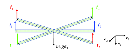
Figure 2: Multiple equilibria for $t_{0}=0$.

The internal force $t_{0}<0$ corresponds to the situation that the two quadrotors move closer to the middle of the pipe, which is quite dangerous due to the risk of drone collision. Therefore, we choose $t_{0}>0$ as the desired internal force shown in Fig. 3, and the uniqueness of $t_{0}$ is guaranteed by the horizontal formation setting.

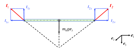
Figure 3: Unique equilibrium for $t_{0}>0$.

Remark 2.

In Fig. 3, since the payload is at its equilibrium, all the forces on the payload intersect at a common point (planar pencil [35]), constituting three-component force balance.

IV-C Force-coordination Formation Control Framework

If the cable lengths are known, we can configure out the desired trajectories of the quadrotors to keep the pipe parallel to the ground. However, without knowing the cable lengths, the average load distribution cannot be achieved by the preset configuration planning. Therefore, a force-coordination formation control framework is proposed to overcome this limitation. The controller structure is shown in Fig. 4.

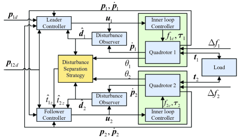
Figure 4: Controller structure for force-coordination control.

For the two quadrotors, the controllers can be decomposed into two parts: one part is to keep the horizontal formation and the other is to achieve force-consensus in the vertical direction.

IV-C1 Formation keeping in the horizontal plane

The leader-follower control laws for keeping the formation in the horizontal plane are designed based on (16) as

$$\bm{u}_{1xy} =\bm{G}(-k_{1}\tilde{\bm{p}}_{12}-k_{2}\dot{\tilde{\bm{p}}}_{12}+\bm{\pi}_{1}-g\bm{e}_{3}-\hat{\bm{d}}_{1})$$ (34)

$$\bm{u}_{2xy} =\bm{G}(\quad k_{1}\tilde{\bm{p}}_{12}+k_{2}\dot{\tilde{\bm{p}}}_{12}-g\bm{e}_{3}-\hat{\bm{d}}_{2})$$

where $\bm{u}_{ixy}$ is the projection of the controller $\bm{u}_{i}$ in (16) into the horizontal plane, with $\bm{G}=[\bm{e}_{1},\bm{e}_{2}]^{\top}\in\mathbb{R}^{2\times 3}$.

IV-C2 Force-consensus in the vertical direction

According to the definition (4), the vertical force-consensus error $t_{2z}-t_{1z}$ can be calculated as

$$t_{2z}-t_{1z} =\bm{e}_{3}^{\top}(m_{2}\bm{d}_{2}-m_{1}\bm{d}_{1}+\bm{\Xi})$$ (35)

where $\bm{\Xi}=\Delta f_{2}\bm{R}_{2}\bm{e}_{3}-\Delta f_{1}\bm{R}_{1}\bm{e}_{3}\in\mathbb{R}^{3}$ is the difference between the thrust uncertainties of two quadrotors.

Using the lumped disturbance estimates, the estimate for the vertical force-consensus error can be expressed as

$$\hat{t}_{2z}-\hat{t}_{1z}=\bm{e}_{3}^{\top}(m_{2}\hat{\bm{d}}_{2}-m_{1}\hat{\bm{d}}_{1}+\hat{\bm{\Xi}})$$ (36)

where $\hat{t}_{iz}\in\mathbb{R}$ is the estimate of the $i$th cable force in the vertical direction and $\hat{\bm{\Xi}}=[\hat{\Xi}_{x},\hat{\Xi}_{y},\hat{\Xi}_{z}]\in\mathbb{R}^{3}$ is the estimate of $\bm{\Xi}$.

For quadrotor 1, the controller in the vertical direction is designed only for height maintenance as below

$$u_{1z}=-k_{3}(p_{1z}-p_{1dz})-k_{4}\dot{p}_{1z}-g-\hat{d}_{1z}.$$ (37)

For quadrotor 2, the controller in the vertical direction is designed to achieve vertical force consensus between two quadrotors as

$$u_{2z}= -k_{4}\dot{p}_{2z}-g-\hat{d}_{2z}+k_{f}(\hat{t}_{2z}-\hat{t}_{1z})$$ (38)

$$= -k_{4}\dot{p}_{2z}-g-\hat{d}_{2z}+k_{f}(m_{2}\hat{d}_{2z}-m_{1}\hat{d}_{1z}+\hat{\Xi}_{z})$$

where $k_{f}\in\mathbb{R}^{+}$ is the force-consensus gain.

In summary, the whole leader-follower controller for the $i$th quadrotor is expressed as

$$\bm{u}_{i}=\begin{bmatrix}\bm{u}_{ixy}^{\top}&u_{iz}\end{bmatrix}^{\top}$$ (39)

where $\hat{\Xi}_{z}$ in $u_{2z}$ cannot be obtained directly from disturbance estimation, and the detailed estimation method for $\hat{\Xi}_{z}$ will be developed in the next subsection.

Remark 3.

More complex manipulations of the pipe beyond averaging load distribution through force-consensus can be realized using the proposed force-coordination control framework by pre-planned force trajectories for the vehicles, which is similar to the method in [23].

IV-D Disturbance Separation under Quasi-static Condition

Quadrotors are underactuated systems that need to rotate to adjust their thrust directions. Therefore, we can introduce the horizontal force balance equations under the quasi-static condition to obtain $\Delta\hat{f}_{i}$, and then separate it from the lumped disturbance estimate $\hat{\bm{d}}_{i}$ for the precise estimate of the cable force $\bm{t}_{i}$. According to equation (36), the better the estimation for $\hat{\Xi}_{z}$, the smaller the force-consensus error. The quasi-static condition refers to the situation that the velocity of the payload changes slowly, i.e.,

$$\ddot{\bm{p}}_{0}\approx\bm{0}_{3\times 1}$$ (40)

which is reasonable during the transportation process.

Without loss of generality, the quadrotors-payload structure is assumed to stay in the XZ plane of NED frame under the quasi-static condition in this scenario. Substituting $\ddot{\bm{p}}_{0}=\bm{0}_{3\times 1}$ into the payload dynamics (1) yields

$$t_{1x}+t_{2x} =0$$ (41)

$$t_{1z}+t_{2z} =m_{0}g.$$

To be explicit, according the definitions in (4) and (13), the disturbance estimate $\hat{\bm{d}}_{i}$ satisfies the following relation:

$$\hat{\bm{d}}_{i} =\bm{d}_{i}+\tilde{\bm{d}}_{i}$$ (42)

$$=-\frac{\Delta f_{i}}{m_{i}}\bm{R}_{i}\bm{e}_{3}+\frac{1}{m_{i}}\bm{t}_{i}+\tilde{\bm{d}}_{i}.$$

The attitude of the $i$th quadrotor can be represented by the Euler angles $(\phi_{i},\theta_{i},\psi_{i})$, and the rotation matrix $\bm{R}_{i}$ can be expressed as

$$\bm{R}_{i} =\bm{R}_{z}(0)\bm{R}_{y}(\theta_{i})\bm{R}_{x}(\phi_{i})$$ (43)

$$=\begin{bmatrix}\cos\theta_{i}&\sin\phi_{i}\sin\theta_{i}&\cos\phi_{i}\sin\theta_{i}\\ 0&\cos\phi_{i}&-\sin\phi_{i}\\ -\sin\theta_{i}&\sin\phi_{i}\cos\theta_{i}&\cos\phi_{i}\cos\theta_{i}\end{bmatrix}$$

where $\psi_{i}$ is set as zero. Expanding (42) yields

$$\begin{bmatrix}\hat{d}_{ix}\\ \hat{d}_{iz}\end{bmatrix}=\frac{1}{m_{i}}\begin{bmatrix}-\Delta f_{i}\sin\theta_{i}\cos\phi_{i}+t_{ix}+m_{i}\tilde{d}_{ix}\\ -\Delta f_{i}\cos\theta_{i}\cos\phi_{i}+t_{iz}+m_{i}\tilde{d}_{iz}\end{bmatrix}.$$ (44)

For notation simplicity, the following substitutions are adopted

$$\hat{\Delta}_{x} =m_{1}\hat{d}_{1x}+m_{2}\hat{d}_{2x}$$ (45)

$$\hat{\Delta}_{z} =m_{1}\hat{d}_{1z}+m_{2}\hat{d}_{2z}-m_{0}g$$

$$\tilde{\Delta}_{x} =m_{1}\tilde{d}_{1x}+m_{2}\tilde{d}_{2x}$$

$$\tilde{\Delta}_{z} =m_{1}\tilde{d}_{1z}+m_{2}\tilde{d}_{2z}$$

where $\hat{\Delta}_{x}$ and $\hat{\Delta}_{z}$ denote the estimate results, $\tilde{\Delta}_{x}$ and $\tilde{\Delta}_{z}$ denote the estimation errors.

Combining (41) and (44), the thrust uncertainties under the quasi-static condition can be obtained as

$$\Delta f_{1} =\frac{\hat{\Delta}_{x}-\hat{\Delta}_{z}\tan\theta_{2}-\tilde{\Delta}_{x}+\tilde{\Delta}_{z}\tan\theta_{2}}{(\cos\theta_{1}\tan\theta_{2}-\sin\theta_{1})\cos\phi_{1}}$$ (46)

$$\Delta f_{2} =\frac{\hat{\Delta}_{x}-\hat{\Delta}_{z}\tan\theta_{1}-\tilde{\Delta}_{x}+\tilde{\Delta}_{z}\tan\theta_{1}}{(\cos\theta_{2}\tan\theta_{1}-\sin\theta_{2})\cos\phi_{2}}$$

so that $\Xi_{z}$ is derived as

$$\Xi_{z}=\frac{\left(\hat{\Delta}_{z}-\tilde{\Delta}_{z}\right)\left(\tan\theta_{1}+\tan\theta_{2}\right)-2\left(\hat{\Delta}_{x}-\tilde{\Delta}_{x}\right)}{\tan\theta_{2}-\tan\theta_{1}}.$$ (47)

Then the estimates for the thrust uncertainties $\Delta f_{1}$ and $\Delta f_{2}$ can be obtained by removing the estimation errors $\tilde{\Delta}_{x}$ and $\tilde{\Delta}_{z}$ from equation (46) as

$$\Delta\hat{f}_{1} =\frac{\hat{\Delta}_{x}-\hat{\Delta}_{z}\tan\theta_{2}}{(\cos\theta_{1}\tan\theta_{2}-\sin\theta_{1})\cos\phi_{1}}$$ (48)

$$\Delta\hat{f}_{2} =\frac{\hat{\Delta}_{x}-\hat{\Delta}_{z}\tan\theta_{1}}{(\cos\theta_{2}\tan\theta_{1}-\sin\theta_{2})\cos\phi_{2}}.$$

Based on equation (47), the estimate $\hat{\Xi}_{z}$ and the estimation error $\tilde{\Xi}_{z}$ can be expressed separately as

$$\hat{\Xi}_{z}=\frac{\left(\tan\theta_{1}+\tan\theta_{2}\right)\hat{\Delta}_{z}-2\hat{\Delta}_{x}}{\tan\theta_{2}-\tan\theta_{1}}$$ (49)

and

$$\tilde{\Xi}_{z} =\frac{\left(\tan\theta_{1}+\tan\theta_{2}\right)\tilde{\Delta}_{z}-2\tilde{\Delta}_{x}}{\tan\theta_{2}-\tan\theta_{1}}.$$ (50)

The vertical cable force estimate $\hat{t}_{iz}$ can be calculated according to equation (44) as

$$\hat{t}_{iz}=m_{i}\hat{d}_{iz}+\Delta\hat{f}_{i}\cos\theta_{i}\cos\phi_{i}$$ (51)

which equals to the actual vertical cable force $t_{iz}$ when the estimation error $\tilde{d}_{iz}$ converges to zero.

Finally, the controller (38) for force-consensus in the vertical direction is made feasible under the quasi-static condition.

Remark 4.

Assuming that precise disturbance estimation is achieved, i.e., $\tilde{\bm{d}}_{i}\approx\bm{0}_{3\times 1}$, there are six unknown variables $\Delta f_{i}$, $t_{ix}$ and $t_{iz}$, $i=1,2$, which can be solved from six equations by combining equation (41) and equation (44).

IV-E Stability Analysis

For the stability of quadrotor 1 in the vertical direction, by substituting (37) into (5), the tracking error dynamics satisfies

$$\ddot{\tilde{p}}_{1z}=-k_{4}\dot{\tilde{p}}_{1z}-k_{3}\tilde{p}_{1z}-\tilde{d}_{1z}$$ (52)

from which the exponential convergence of $\tilde{p}_{1z}$ can be obtained when the disturbance estimation error $\tilde{d}_{1z}\approx 0$. Therefore, the height of quadrotor 1 can be held.

As is shown in Fig. 5, the pitch angle of the pipe is denoted as $\theta_{0}$, and the desired position of quadrotor 2 is denoted as $p_{2d}$, corresponding to zero pitch angle of the pipe. When the height of quadrotor 1 and the desired horizontal relative position are fixed, $p_{2d}$ is a unique equilibrium according to the analysis in Section IV-B, so that the desired vertical position of quadrotor 2 can be seen as fixed, i.e., $\dot{p}_{2dz}=\ddot{p}_{2dz}=0$.

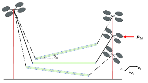
Figure 5: Force-consensus regulation in the vertical direction.

We require that the desired horizontal relative position between the two quadrotors satisfies

$$\|\bm{p}_{12dxy}\|>2l_{0}$$ (53)

so that the internal force in the pipe is always positive $(t_{0}>0)$. This formation configuration also guarantees that the pitch angles for the two quadrotors, $\theta_{1}$ and $\theta_{2}$, have lower and upper bounds, i.e.,

$$0< \underline{\theta}_{1}\leq\theta_{1}\leq\overline{\theta}_{1}<\frac{\pi}{2}$$ (54)

$$-\frac{\pi}{2}< \underline{\theta}_{2}\leq\theta_{2}\leq\overline{\theta}_{2}<0.$$

Under the quasi-static condition, the cable forces can be computed as [23]

$$\bm{t}_{1} =\left[\frac{t_{0}\cos\theta_{0}}{2},0,\frac{-t_{0}\sin\theta_{0}+m_{0}g}{2}\right]^{\top}$$ (55)

$$\bm{t}_{2} =\left[-\frac{t_{0}\cos\theta_{0}}{2},0,\frac{t_{0}\sin\theta_{0}+m_{0}g}{2}\right]^{\top}.$$

The following equation is obtained in the vertical direction

$$t_{2z}-t_{1z}=t_{0}\sin\theta_{0}.$$ (56)

Then using (35), (36), and (50), the force-consensus error in the vertical direction is estimated as

$$\hat{t}_{2z}-\hat{t}_{1z} =t_{2z}-t_{1z}+m_{2}\tilde{d}_{2z}-m_{1}\tilde{d}_{1z}+\tilde{\Xi}_{z}$$ (57)

$$=t_{0}\sin\theta_{0}+\bm{C}\tilde{\bm{d}}$$

where $\bm{C}=\left[\frac{-2m_{1}}{\tan\theta_{2}-\tan\theta_{1}},0,\frac{2m_{1}\tan\theta_{1}}{\tan\theta_{2}-\tan\theta_{1}},\frac{-2m_{2}}{\tan\theta_{2}-\tan\theta_{1}},0,\right.\\ \left.\frac{2m_{2}\tan\theta_{2}}{\tan\theta_{2}-\tan\theta_{1}}\right]$ and $\tilde{\bm{d}}$ is notated in (22).

The vertical position and vertical velocity tracking error of quadrotor 2 are denoted by the notations $(\tilde{p}_{2z},\dot{\tilde{p}}_{2z})$. Combining (5), (38), and (57), the tracking error dynamics for quadrotor 2 in the vertical direction is

$$\ddot{\tilde{p}}_{2z} =-k_{4}\dot{\tilde{p}}_{2z}-\tilde{d}_{2z}+k_{f}t_{0}\sin\theta_{0}+k_{f}\bm{C}\tilde{\bm{d}}.$$ (58)

Lemma 1.

$t_{0}\sin\theta_{0}$ and $\tilde{p}_{2z}$ are negatively correlated and satisfy the following equation

$$t_{0}\sin\theta_{0}=-\sigma\left(\tilde{p}_{2z}\right)$$ (59)

where $\sigma(x)$ is a strictly increasing function with $\sigma\left(0\right)=0$. Moreover, the slope of $\sigma(x)$ satisfies

$$0<\underline{\sigma}<\frac{d\sigma(x)}{dx}<\overline{\sigma}$$ (60)

where $\underline{\sigma}\in\mathbb{R}^{+}$ and $\overline{\sigma}\in\mathbb{R}^{+}$ are the constant lower and upper bounds.

Proof.

Detailed proof can be found in the supplementary material. ∎

Based on Lemma 1, equation (58) can be turned into

$$\ddot{\tilde{p}}_{2z}=-k_{4}\dot{\tilde{p}}_{2z}-k_{f}t_{0}\sigma\left(\tilde{p}_{2z}\right)+\bm{D}\tilde{\bm{d}}$$ (61)

where $\bm{D}=\left[\frac{-2k_{f}m_{1}}{\tan\theta_{2}-\tan\theta_{1}},0,\frac{2k_{f}m_{1}\tan\theta_{1}}{\tan\theta_{2}-\tan\theta_{1}},\frac{-2k_{f}m_{2}}{\tan\theta_{2}-\tan\theta_{1}},0,\right.\\ \left.\frac{\left(2k_{f}m_{2}-1\right)\tan\theta_{2}+\tan\theta_{1}}{\tan\theta_{2}-\tan\theta_{1}}\right]$. According to (54), there exists unknown positive constant $\bar{D}$ satisfying

$$\|\bm{D}\|\leq\bar{D}.$$ (62)

Here the boundedness of $\|\bm{D}\|$ can be derived since the absolute value of the denominator $|\tan\theta_{2}-\tan\theta_{1}|$ is lower bounded by the positive constant $|\tan\overline{\theta}_{2}-\tan\underline{\theta}_{1}|$.

Assumption 2.

There exist positive constants $\varepsilon_{1}$, $\gamma$, $k_{4}$, and $k_{f}$ satisfying

$$k_{4} >\varepsilon_{1}+\frac{\overline{t}_{0}}{4\gamma}$$ (63)

$$k_{f} <\frac{\varepsilon_{1}\underline{\sigma}}{\gamma\overline{\sigma}^{2}}$$

where details about $\overline{t}_{0}$, $\overline{\sigma}$ and $\underline{\sigma}$ can be found in the supplementary material.

Theorem 2.

Consider two quadrotors carrying a suspended payload under the quasi-static condition, modeled as (5), with the control laws (39), the disturbance estimate updated as in (12), and the inconsistency between the thrust uncertainties estimated as in (49). Suppose that Assumptions 1-3 hold. Then the signals of the overall closed-loop system, $(\tilde{\bm{p}}_{1xy},\dot{\tilde{\bm{p}}}_{1xy},\tilde{\bm{p}}_{12xy},\dot{\tilde{\bm{p}}}_{12xy})$, ($\tilde{p}_{1z},\dot{\tilde{p}}_{1z},\tilde{p}_{2z},\dot{\tilde{p}}_{2z}$), and ($\tilde{\bm{d}}_{1},\tilde{\bm{d}}_{2}$), are uniformly ultimately bounded.

Proof.

The boundedness of $\tilde{\bm{d}}_{i}$ is already established in (15). The horizontal controller (34) and the vertical controller (37) (38) are designed independently. Since the horizontal controller (34) is the same as that in the position-coordination control scheme, the boundedness of the states in the horizontal plane $(\tilde{\bm{p}}_{1xy},\dot{\tilde{\bm{p}}}_{1xy},\tilde{\bm{p}}_{12xy},\dot{\tilde{\bm{p}}}_{12xy})$ can be proved. In addition, the boundedness of $(\tilde{p}_{1z},\dot{\tilde{p}}_{1z})$ is already established after (52).

We focus on the stability of quadrotor 2 in the vertical direction. Define the Lyapunov function as

$$V=\frac{1}{2}\begin{bmatrix}\tilde{p}_{2z}&\dot{\tilde{p}}_{2z}\end{bmatrix}\begin{bmatrix}k_{4}\varepsilon_{1}&\varepsilon_{1}\\ \varepsilon_{1}&1\end{bmatrix}\begin{bmatrix}\tilde{p}_{2z}\\ \dot{\tilde{p}}_{2z}\end{bmatrix}$$ (64)

where $\varepsilon_{1}\in\mathbb{R}^{+}$ is referred in Assumption 2.

Differentiate (64) with respect to time $t$

$$\dot{V}= \begin{bmatrix}\tilde{p}_{2z}&\dot{\tilde{p}}_{2z}\end{bmatrix}\begin{bmatrix}k_{4}\varepsilon_{1}&\varepsilon_{1}\\ \varepsilon_{1}&1\end{bmatrix}\begin{bmatrix}\dot{\tilde{p}}_{2z}\\ \ddot{\tilde{p}}_{2z}\end{bmatrix}$$ (65)

$$= k_{4}\varepsilon_{1}\tilde{p}_{2z}\dot{\tilde{p}}_{2z}+\varepsilon_{1}\tilde{p}_{2z}\ddot{\tilde{p}}_{2z}+\varepsilon_{1}\dot{\tilde{p}}_{2z}^{2}+\dot{\tilde{p}}_{2z}\ddot{\tilde{p}}_{2z}$$

$$= -k_{f}t_{0}\varepsilon_{1}\tilde{p}_{2z}\sigma\left(\tilde{p}_{2z}\right)-\left(k_{4}-\varepsilon_{1}\right)\dot{\tilde{p}}_{2z}^{2}$$

$$-k_{f}t_{0}\dot{\tilde{p}}_{2z}\sigma\left(\tilde{p}_{2z}\right)+\dot{\tilde{p}}_{2z}\bm{D}\tilde{\bm{d}}+\varepsilon_{1}\tilde{p}_{2z}\bm{D}\tilde{\bm{d}}$$

$$\leq -k_{f}t_{0}\varepsilon_{1}\underline{\sigma}\tilde{p}_{2z}^{2}-\left(k_{4}-\varepsilon_{1}\right)\dot{\tilde{p}}_{2z}^{2}$$

$$-k_{f}t_{0}\dot{\tilde{p}}_{2z}\sigma\left(\tilde{p}_{2z}\right)+\dot{\tilde{p}}_{2z}\bm{D}\tilde{\bm{d}}+\varepsilon_{1}\tilde{p}_{2z}\bm{D}\tilde{\bm{d}}.$$

Using Young’s inequality yields

$$-k_{f}t_{0}\dot{\tilde{p}}_{2z}\sigma\left(\tilde{p}_{2z}\right)\leq \frac{{t}_{0}}{4\gamma}\dot{\tilde{p}}_{2z}^{2}+\gamma k_{f}^{2}t_{0}\sigma^{2}\left(\tilde{p}_{2z}\right)$$ (66)

$$\leq \frac{{t}_{0}}{4\gamma}\dot{\tilde{p}}_{2z}^{2}+\gamma k_{f}^{2}t_{0}\overline{\sigma}^{2}\tilde{p}_{2z}^{2}$$

where $\gamma\in\mathbb{R}^{+}$ is the tuning parameter.

Therefore, $\dot{V}$ satisfies

$$\dot{V}\leq -\left(k_{f}t_{0}\varepsilon_{1}\underline{\sigma}-\gamma k_{f}^{2}t_{0}\overline{\sigma}^{2}\right)\tilde{p}_{2z}^{2}-\left(k_{4}-\varepsilon_{1}-\frac{t_{0}}{4\gamma}\right)\dot{\tilde{p}}_{2z}^{2}$$ (67)

$$+\|\dot{\tilde{p}}_{2z}\|\|\bm{D}\|\|\tilde{\bm{d}}\|+\varepsilon_{1}\|\tilde{p}_{2z}\|\|\bm{D}\|\|\tilde{\bm{d}}\|$$

$$\leq -k_{f}t_{0}\left(\varepsilon_{1}\underline{\sigma}-\gamma k_{f}\overline{\sigma}^{2}\right)\tilde{p}_{2z}^{2}-\left(k_{4}-\varepsilon_{1}-\frac{t_{0}}{4\gamma}\right)\dot{\tilde{p}}_{2z}^{2}$$

$$+\sqrt{2}\bar{D}\bar{\tilde{d}}\|\dot{\tilde{p}}_{2z}\|+\sqrt{2}\varepsilon_{1}\bar{D}\bar{\tilde{d}}\|\tilde{p}_{2z}\|$$

where $\|\tilde{\bm{d}}\|\leq\sqrt{2}\bar{\tilde{d}}$ is used. According to Lyapunov bounded theory [33], the error variables $\left(\tilde{p}_{2z},\dot{\tilde{p}}_{2z}\right)$ are uniformly ultimately bounded if (63) is satisfied. ∎

V Numerical Simulations

Numerical simulation is carried out first to validate the proposed force-coordination control strategy. Specially, cables of different unknown lengths and different thrust uncertainties are configured for the two quadrotors to demonstrate the effects of disturbance separation and force-consensus. In simulation, the cables are assumed to be massless links and the cable forces are modeled following [13]. System and control parameters are listed in Table I. The thrust uncertainties for the two quadrotors are set as $\Delta f_{1}=-0.2f_{1c}$ and $\Delta f_{2}=-0.4f_{2c}$, respectively. The simulation time is set as 30 seconds. Quadrotor 2 is free to adjust its height to achieve force-consensus. According to the equilibrium analysis in Section IV-B, the pipe will eventually become parallel to the ground.

TABLE I: Parameters used in the simulation

System Parameters
$m_{i}$	i = 0	$0.44,\mathrm{kg}$
	i = 1	$0.87,\mathrm{kg}$
	i = 2	$0.88,\mathrm{kg}$
$\bm{J}_{i}$	i = 0	$\mathrm{diag}\{0.0035,0.15,0.15\},\mathrm{kg}\cdot\mathrm{m}^{2}$
	i = 1	$\mathrm{diag}\{0.003,0.003,0.004\},\mathrm{kg}\cdot\mathrm{m}^{2}$
	i = 2	$\mathrm{diag}\{0.003,0.003,0.004\},\mathrm{kg}\cdot\mathrm{m}^{2}$
$l_{i}$	i = 0	$1.0,\mathrm{m}$
	i = 1	$0.8,\mathrm{m}$
	i = 2	$0.4,\mathrm{m}$
Control Parameters
$k_{1},k_{2},k_{3},k_{4}$		$4,4,5,8$
$k_{f}$		$0.5$
$\iota$		$5$
Initial Conditions
$\bm{p}_{0}(0)$		$[0,0,0]^{\top},\mathrm{m}$
$\bm{p}_{1}(0)$		$[1.4,0.12,-0.68]^{\top},\mathrm{m}$
$\bm{p}_{2}(0)$		$[-1.14,0,-0.38]^{\top},\mathrm{m}$
$\dot{\bm{p}}_{i}(0)$, $i=0,1,2$		$[0,0,0]^{\top},\mathrm{m/s}$
$\bm{R}_{i}(0)$, $i=0,1,2$		$[\bm{e}_{1},\bm{e}_{2},\bm{e}_{3}]$
$\bm{\Omega}_{i}(0)$, $i=0,1,2$		$[0,0,0]^{\top},\mathrm{rad/s}$
$\bm{z}_{i}(0)$, $i=1,2$		$[0,0,0]^{\top}$
Desired Trajectories
$\bm{p}_{1d}$		$[1,0,-1]^{\top},\mathrm{m}$
$\bm{p}_{12dxy}$		$[2.5,0]^{\top},\mathrm{m}$

To test the stability of the equilibrium, the aerial transportation system works in the position-coordination control mode in the first 10 seconds, so the pipe leans towards approximately $-10^{\circ}$ in the end as shown in Fig. 7. Then the controllers switch to the force-coordination mode. Since quadrotor 2 has the shorter cable, it burdens more pipe weight than quadrotor 1 under the position-consensus condition. Once in the force-coordination mode, quadrotor 2 comes down slowly, making the pipe finally parallel to the ground as shown in Fig. 6, which implies the stability of the equilibrium.

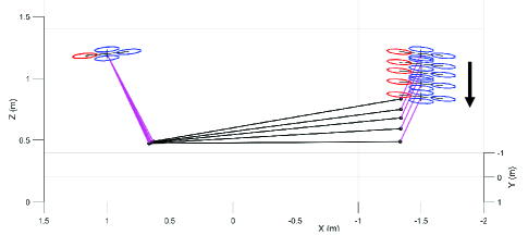
Figure 6: Movement snapshots of force-consensus simulation.

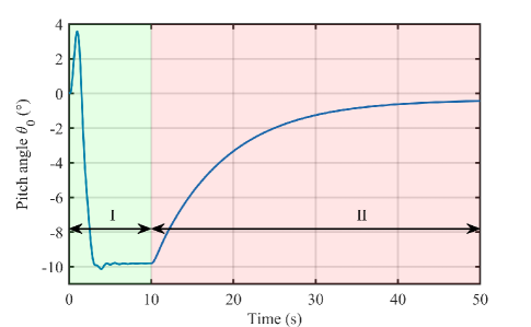
Figure 7: Pitch angle $\theta_{0}$ of the pipe. Stage i@ stands for the position-coordination period and Stage ii@ stands for the force-coordination period.

The estimation errors of vertical cable forces are presented in Fig. 8. The bounded convergence property is exhibited. Subject to the disturbance estimation error $\tilde{\bm{d}}_{i}$, both the cable force estimation error in Fig. 8 and the pitch angle in Fig. 7 can only converge to a small neighborhood of zero.

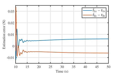
Figure 8: Estimation errors of the vertical cable forces.

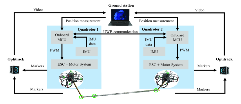
Figure 9: Experimental platform structure.

VI Experiment Validation

To demonstrate the effectiveness of the proposed force-coordination algorithm in practical implementation, real-world flight tests are performed in an indoor flight test environment. The test facility consists of Optitrack motion capture system, ground station, and quadrotor platforms, as shown in Fig. 9, which has been used to support different research projects (see e.g., [36, 37, 38] for details). The first test is intended to illustrate the significant inconsistency of the thrust uncertainties between the two quadrotors, followed by the main test for the aerial transportation system.

System and control parameters are listed in Table II. Due to the measurement noises, the disturbance observer gain $\iota$ cannot be selected too large. Otherwise, it will result in large chattering in the disturbance estimate, which may lead to sudden and large swings of the quadrotor. The force-consensus gain $k_{f}$ is selected small as well.

TABLE II: Parameters used in the experiments

System Parameters
$m_{i}$	i = 0	$0.745,\mathrm{kg}$
	i = 1	$0.831,\mathrm{kg}$
	i = 2	$0.832,\mathrm{kg}$
$\bm{J}_{i}$	i = 1	$\mathrm{diag}\{0.003,0.003,0.004\},\mathrm{kg}\cdot\mathrm{m}^{2}$
	i = 2	$\mathrm{diag}\{0.003,0.003,0.004\},\mathrm{kg}\cdot\mathrm{m}^{2}$
$l_{i}$	i = 0	$1.0,\mathrm{m}$
	i = 1	$0.7,\mathrm{m}$
	i = 2	$0.3,\mathrm{m}$
Control Parameters
$k_{1},k_{2},k_{3},k_{4}$		$4,4,5,8$
$k_{f}$		$0.1$
$\iota$		$1.2$
Desired Trajectories
$\bm{p}_{1d}$		$[1.5,0,-1.2]^{\top},\mathrm{m}$
$\bm{p}_{12dxy}$		$[2.5,0]^{\top},\mathrm{m}$

VI-A Hovering experiment

Two quadrotors carrying objects of similar weight are required to hover at the same height. Specifically, quadrotor 1 carries a payload of $0.248\mathrm{kg}$ and quadrotor 2 carries a payload of $0.252\mathrm{kg}$. We adopt the disturbance observer based position controller for both quadrotors. The desired height for the two quadrotors are chosen as $1.2\mathrm{m}$.

According to the definition (3) and the model (5), under the hovering condition of $\ddot{\bm{p}}_{i}=\bm{0}_{3\times 1}$, the actual values of the lumped disturbances in the vertical direction for the two quadrotors can be approximately computed as $m_{i}d_{iz}=-m_{i}g+f_{ic}$. It can be observed from Fig. 10 that the disturbance estimate $m_{i}\hat{d}_{iz}$ converges to a small neighborhood of the actual value $m_{i}d_{iz}$, implying the effectiveness of the disturbance observer. Although the whole weight of the two quadrotor-payload units are almost same, $m_{2}d_{2z}$ is nearly $1\mathrm{N}$ larger than $m_{1}d_{1z}$. It can inferred that the inconsistency of the thrust uncertainties between the two quadrotors reaches about $10\%$ of the total gravity and $40\%$ of the payload gravity (whole weight of quadrotor 1 with payload is 1.079kg and payload is 0.248kg), which implies that even drones of the same type may have severe inconsistency of uncertainties. According to the experimental experience, this inconsistency may be amplified by the differences between battery levels. In this case, it is unfeasible to apply the force control methods proposed in [22] or [23]. Therefore, we have to separate the cable force from the lumped disturbance for force-coordination control.

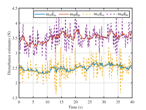
Figure 10: Disturbance estimates in the vertical direction.

VI-B Force-consensus-based experiment

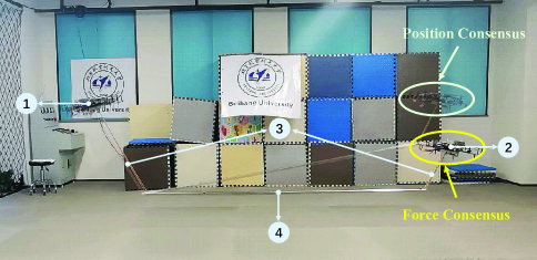
Figure 11: 1) quadrotor 1 acting as the leader; 2) quadrotor 2 acting as the follower; 3) cables of different lengths; 4) the steel pipe

The experiment configuration is shown in Fig. 9. Quadrotor 1 is required to hover at the desired position $\bm{p}_{1d}$, while quadrotor 2 is commanded to maintain the desired horizontal relative position $\bm{p}_{12dxy}$ and achieve force-consensus in the vertical direction. The choice of $\bm{p}_{12d}$ is based on the requirement that $\|\bm{p}_{12dxy}\|$ has to be larger than the length of the pipe as explained in (53) and less than the sum of the lengths of the cables and the length of the pipe, i.e., $2l_{0}<\|\bm{p}_{12dxy}\|<2l_{0}+l_{1}+l_{2}$.

Same as in the simulation studies, the experiment also starts from position-coordination control mode and then changes to force-coordination control mode at $10$s. The position tracking errors of quadrotor 1 and quadrotor 2 are shown respectively in Fig. 12 and Fig. 13. It can be observed that the position tracking errors fluctuate in the range of $0.02\mathrm{m}$ roughly. Therefore, combining with the estimation results shown in Fig. 10, the robustness of the DO-based controller to the lumped disturbance is well demonstrated.

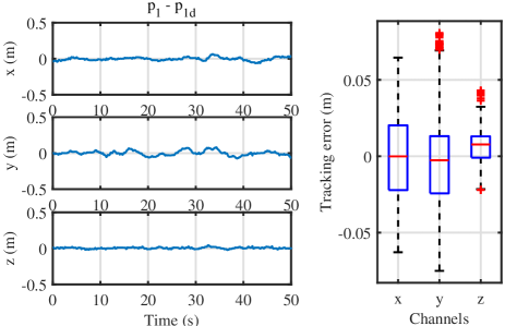
Figure 12: Tracking performance of quadrotor 1.

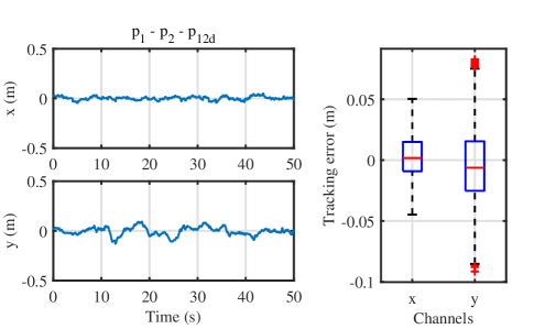
Figure 13: Formation-keeping performance of quadrotor 2.

The estimates of thrust uncertainties $\Delta f_{1}$ and $\Delta f_{2}$ are shown in Fig. 14. It can be observed that the thrust uncertainty estimate $\Delta\hat{f}_{2}$ for quadrotor 2 is larger than $\Delta\hat{f}_{1}$ for quadrotor 1, which matches with the comparison result in the hovering experiment. The evolution of the pitch angle $\theta_{0}$ of the pipe is shown in Fig. 15. During the first 10 seconds, the pipe keeps static at the inclined posture of $\theta_{0}\approx-14^{\circ}$. In the subsequent force-coordination control mode, the pipe approaches the equilibrium of the horizontal posture gradually, as quadrotor 2 goes down slowly over 20 seconds. Actually, even though the dominant thrust uncertainty has been removed from the lumped force disturbance estimate, there are still some extra trivial uncertainties existing in the residual disturbance estimate, which is regarded as the vertical cable force estimate $\hat{t}_{iz}$. As a result, the final pitch angle $\theta_{0}$ of the pipe can only stay in the interval of $1^{\circ}$ and $3^{\circ}$. Here the extra model uncertainties refer to the mass of the cable, the deviation of the CoM of the quadrotor, the acceleration of the pipe, and the turbulence in the test area, which are usually small compared to the thrust uncertainty, so that they are neglected in this study.

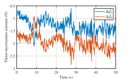
Figure 14: Estimates of the thrust uncertainties.

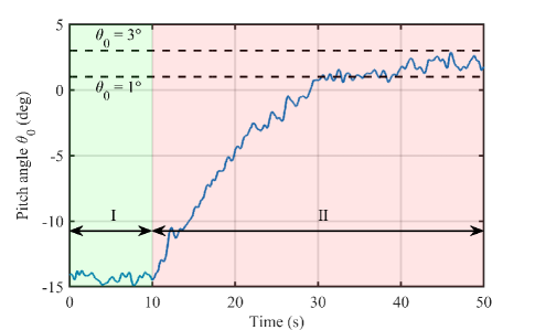
Figure 15: Pitch angle $\theta_{0}$ of the pipe. Stage i@ stands for the position-coordination period and Stage ii@ stands for the force-coordination period.

VII Conclusions

In this article, a force-coordination control scheme with disturbance separation and estimation is proposed, as demonstrated for a collaborative transportation system. Compared to position-coordination control, force-coordination control can provide more complex manipulation of the payload than simply moving along the predefined trajectory. Under the quasi-static condition, the force-consensus objective can ensure that vehicles share the same weight of the payload, which can extend the endurance of the entire transportation mission. By exploiting the intrinsic force balance conditions of the cooperative quadrotors, thrust uncertainty can be separately estimated from the lumped force disturbance. Therefore, a more accurate cable force estimate can be obtained by removing thrust uncertainty. This overcomes the problem that the existing disturbance estimation methods cannot distinguish the different disturbances in the same channel. Simulation results verify the effectiveness of the proposed method and experiments further demonstrate that the proposed method can achieve good performance in practical implementation of payload transportation using heterogeneous quadrotors. Future research directions include payload attitude control through force-coordination and separating other undesirable force disturbances, such as wind.

Supplemental Material: Sector Bounds for Vertical Cable Force Error in Cable-Suspended Load Transportation System

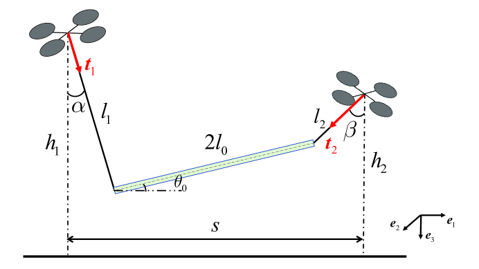
Figure 16: Regulation of the height of quadrotor 2.

VII-A Proof for Lemma 1

Proof.

First, considering the scene where the internal force $t_{0}>0$, the cable angles $\alpha,\beta$ and the load angle $\theta_{0}$ in Fig. 16 satisfy

$$0<\alpha<\frac{\pi}{2},\quad 0<\beta<\frac{\pi}{2},\quad-\frac{\pi}{2}<\theta_{0}<\frac{\pi}{2}.$$ (68)

As the payload stays in the XZ plane of NED frame under the quasi-static condition, the cable forces can be computed as [23]

$$\bm{t}_{1} =\left[\frac{t_{0}\cos\theta_{0}}{2},0,\frac{-t_{0}\sin\theta_{0}+m_{0}g}{2}\right]^{\top},\quad\bm{t}_{2}=\left[-\frac{t_{0}\cos\theta_{0}}{2},0,\frac{t_{0}\sin\theta_{0}+m_{0}g}{2}\right]^{\top}$$ (69)

where $\theta_{0}$ is the pitch angle of the pipe notated in Fig. 16.

From (69), trigonometric functions of $\alpha$ and $\beta$ are computed as

$$\cos\alpha= \frac{-t_{0}\sin\theta_{0}+m_{0}g}{\sqrt{\left(t_{0}\cos\theta_{0}\right)^{2}+\left(-t_{0}\sin\theta_{0}+m_{0}g\right)^{2}}} =\frac{k-\sin\theta_{0}}{g_{1}}$$ (70)

$$\cos\beta= \frac{t_{0}\sin\theta_{0}+m_{0}g}{\sqrt{\left(t_{0}\cos\theta_{0}\right)^{2}+\left(t_{0}\sin\theta_{0}+m_{0}g\right)^{2}}} =\frac{k+\sin\theta_{0}}{g_{2}}$$

$$\sin\alpha= \frac{t_{0}\cos\theta_{0}}{\sqrt{\left(t_{0}\cos\theta_{0}\right)^{2}+\left(-t_{0}\sin\theta_{0}+m_{0}g\right)^{2}}} =\frac{\cos\theta_{0}}{g_{1}}$$

$$\sin\beta= \frac{t_{0}\cos\theta_{0}}{\sqrt{\left(t_{0}\cos\theta_{0}\right)^{2}+\left(t_{0}\sin\theta_{0}+m_{0}g\right)^{2}}} =\frac{\cos\theta_{0}}{g_{2}}$$

where $k=\frac{m_{0}g}{t_{0}}$, $g_{1}=\sqrt{k^{2}-2k\sin\theta_{0}+1}$, and $g_{2}=\sqrt{k^{2}+2k\sin\theta_{0}+1}$ are used for substitutions. Here the derivatives of $g_{1}$ and $g_{2}$ with respect to $\theta_{0}$ are computed as

$$\frac{dg_{1}}{d\theta_{0}} =\frac{1}{g_{1}}\left[(k-\sin\theta_{0})\frac{dk}{d\theta_{0}}-k\cos\theta_{0}\right],\quad\frac{dg_{2}}{d\theta_{0}}=\frac{1}{g_{2}}\left[(k+\sin\theta_{0})\frac{dk}{d\theta_{0}}+k\cos\theta_{0}\right].$$ (71)

The internal force $t_{0}$ satisfies the following constraint equation

$$l_{1}\sin\alpha+l_{2}\sin\beta+2l_{0}\cos\theta_{0}=s.$$ (72)

Using the substitutions in (70) yields

$$l_{1}\frac{\cos\theta_{0}}{g_{1}}+l_{2}\frac{\cos\theta_{0}}{g_{2}}+2l_{0}\cos\theta_{0}=s.$$ (73)

The constraint equation (73) is a high-order equation with respect to $k$, so it is quite hard to express the variable $k$ as an analytic function of $\theta_{0}$. Differentiating (73) with respect to $\theta_{0}$ yields

$$\frac{l_{1}}{g_{1}^{3}}[(k-\sin\theta_{0})\frac{dk}{d\theta_{0}}-k\cos\theta_{0}]+\frac{l_{2}}{g_{2}^{3}}[(k+\sin\theta_{0})\frac{dk}{d\theta_{0}}+k\cos\theta_{0}]=-\frac{s\cdot\sin\theta_{0}}{\cos^{2}\theta_{0}}.$$ (74)

Combining (73), the derivative of $k$ with respect to $\theta_{0}$ is computed as

$$\frac{dk}{d\theta_{0}}=-\frac{\frac{l_{1}}{g_{1}^{3}}(k-\sin\theta_{0})(k\sin\theta_{0}-1)+\frac{l_{2}}{g_{2}^{3}}(k+\sin\theta_{0})(k\sin\theta_{0}+1)+2l_{0}\sin\theta_{0}}{\left[\frac{l_{1}(k-\sin\theta_{0})}{g_{1}^{3}}+\frac{l_{2}(k+\sin\theta_{0})}{g_{2}^{3}}\right]\cos\theta_{0}}$$ (75)

Next, the height of quadrotor 2 is calculated as

$$h_{2} =l_{2}\cos\beta+2l_{0}\sin\theta_{0}-l_{1}\cos\alpha+h_{1}$$ (76)

$$=l_{2}\frac{k+\sin\theta_{0}}{g_{2}}+2l_{0}\sin\theta_{0}-l_{1}\frac{k-\sin\theta_{0}}{g_{1}}+h_{1}$$

where $h_{1}=-p_{1z}$ is assumed to be static at the steady state. The lengths of cables $l_{1}$, $l_{2}$ and the length of pipe $2l_{0}$ are also fixed. Then $h_{2}$ can be seen as a continuous function of $\theta_{0}$. Differentiating $h_{2}$ with respect to $\theta_{0}$ yields

$$\frac{dh_{2}}{d\theta_{0}} =l_{2}\frac{(\frac{dk}{d\theta_{0}}+\cos\theta_{0})g_{2}-(k+\sin\theta_{0})\frac{dg_{2}}{d\theta_{0}}}{g_{2}^{2}}-l_{1}\frac{(\frac{dk}{d\theta_{0}}-\cos\theta_{0})g_{1}-(k-\sin\theta_{0})\frac{dg_{1}}{d\theta_{0}}}{g_{1}^{2}}+2l_{0}\cos\theta_{0}$$ (77)

$$=(\frac{l_{2}}{g_{2}^{3}}-\frac{l_{1}}{g_{1}^{3}})\frac{dk}{d\theta_{0}}\cos^{2}\theta_{0}+\frac{l_{2}\cos\theta_{0}(k\sin\theta_{0}+1)}{g_{2}^{3}}+\frac{l_{1}\cos\theta_{0}(1-k\sin\theta_{0})}{g_{1}^{3}}+2l_{0}\cos\theta_{0}$$

$$=k\cos\theta_{0}\frac{\frac{4l_{1}l_{2}}{g_{1}^{3}g_{2}^{3}}+2l_{0}(\frac{l_{2}}{g_{2}^{3}}+\frac{l_{1}}{g_{1}^{3}})}{\frac{l_{1}(k-\sin\theta_{0})}{g_{1}^{3}}+\frac{l_{2}(k+\sin\theta_{0})}{g_{2}^{3}}}.$$

Since $p_{1dz}$ and $p_{12d}$ are fixed, $p_{2dz}$ is also fixed according to the equilibrium analysis in the article, i.e., $\dot{p}_{2dz}=0$. Therefore, the following equation is obtained

$$\frac{d\tilde{p}_{2z}}{d\theta_{0}}=\frac{d\left(-h_{2}-p_{2dz}\right)}{d\theta_{0}}=-\frac{dh_{2}}{d\theta_{0}}$$ (78)

where $p_{2z}=-h_{2}$ is used. The derivative of the inverse function satisfies

$$\frac{d\theta_{0}}{d\tilde{p}_{2z}}=-\frac{\frac{l_{1}(k-\sin\theta_{0})}{g_{1}^{3}}+\frac{l_{2}(k+\sin\theta_{0})}{g_{2}^{3}}}{k\cos\theta_{0}\left[\frac{4l_{1}l_{2}}{g_{1}^{3}g_{2}^{3}}+2l_{0}(\frac{l_{2}}{g_{2}^{3}}+\frac{l_{1}}{g_{1}^{3}})\right]}.$$ (79)

Finally, differentiating $t_{0}\sin\theta_{0}$ with respect to $\tilde{p}_{2z}$ yields

$$\frac{d(t_{0}\sin\theta_{0})}{d\tilde{p}_{2z}} =\frac{dt_{0}}{d\theta_{0}}\frac{d\theta_{0}}{d\tilde{p}_{2z}}\sin\theta_{0}+\frac{d\sin\theta_{0}}{d\tilde{p}_{2z}}t_{0}$$ (80)

$$=-\frac{dk}{d\theta_{0}}\frac{d\theta_{0}}{d\tilde{p}_{2z}}\frac{m_{0}g\sin\theta_{0}}{k^{2}}+\frac{d\theta_{0}}{d\tilde{p}_{2z}}\frac{m_{0}g\cos\theta_{0}}{k}$$

$$=-\frac{m_{0}g}{k^{3}\cos^{2}\theta_{0}}\frac{\frac{l_{1}}{g_{1}^{3}}(k-\sin\theta_{0})^{2}+\frac{l_{2}}{g_{2}^{3}}(k+\sin\theta_{0})^{2}+2l_{0}\sin^{2}\theta_{0}}{\frac{4l_{1}l_{2}}{g_{1}^{3}g_{2}^{3}}+2l_{0}(\frac{l_{1}}{g_{1}^{3}}+\frac{l_{2}}{g_{2}^{3}})}<0.$$

From which the function $\sigma(\cdot)$ is proved to be strictly increasing. Based on the constraint function (73), the following inequality can be deduced

$$\frac{s}{\cos\theta_{0}}-2l_{0} =\frac{l_{1}}{\sqrt{(k-\sin\theta_{0})^{2}+\cos^{2}\theta_{0}}}+\frac{l_{2}}{\sqrt{(k+\sin\theta_{0})^{2}+\cos^{2}\theta_{0}}}$$ (81)

$$\geq\frac{2\sqrt{2l_{1}l_{2}}}{\sqrt{(k-\sin\theta_{0})^{2}+(k+\sin\theta_{0})^{2}+2\cos^{2}\theta_{0}}}$$

$$=\frac{2\sqrt{l_{1}l_{2}}}{\sqrt{k^{2}+1}}$$

which implies

$$k^{2}\geq\frac{4l_{1}l_{2}}{\left(\frac{s}{\cos\theta_{0}}-2l_{0}\right)^{2}}-1.$$ (82)

Assumption 3.

Consider the pipe suspended by two quadrotors by cables in the XZ plane of NED frame shown in Fig 16, the pitch angle of the pipe $\theta_{0}$ is assumed to satisfy the following bounded condition

$$-\frac{\pi}{2}<-\theta^{*}\leq\theta_{0}\leq\theta^{*}<\frac{\pi}{2}$$ (83)

and the cable angles $\alpha$ and $\beta$ are upper bounded by $\kappa$, i.e.,

$$0<\alpha\leq\kappa<\frac{\pi}{2},\quad\quad 0<\beta\leq\kappa<\frac{\pi}{2},$$ (84)

where $\theta^{*}$ and $\kappa$ are positive constants.

According to the inequality (82), the horizontal distance $s$ can be adjusted to set the lower bound for $k$, i.e.,

$$k\geq\underline{k}=\sqrt{\frac{4l_{1}l_{2}}{\left(\frac{s}{\cos\theta^{*}}-2l_{0}\right)^{2}}-1}>0$$ (85)

where the lower bound $\underline{k}$ corresponds to the upper bound of the internal force $\overline{t}_{0}$.

For the upper bound $\overline{\sigma}$ of $\frac{d\sigma(x)}{dx}$,

$$\frac{d\sigma(x)}{dx}=-\frac{d(t_{0}\sin\theta_{0})}{d\tilde{p}_{2z}} =\frac{m_{0}g}{k^{3}\cos^{3}\theta_{0}}\frac{l_{1}\sin\alpha\cos^{2}\alpha+l_{2}\sin\beta\cos^{2}\beta+2l_{0}\cos\theta_{0}\sin^{2}\theta_{0}}{\frac{4l_{1}l_{2}}{g_{1}^{3}g_{2}^{3}}+2l_{0}\left(\frac{l_{1}}{g_{1}^{3}}+\frac{l_{2}}{g_{2}^{3}}\right)}$$ (86)

$$\leq\frac{m_{0}g}{k^{3}\cos^{2}\theta_{0}}\frac{\left(l_{1}\sin\alpha+l_{2}\sin\beta+2l_{0}\cos\theta_{0}\right)\cdot\max\{\cos^{2}\alpha,\cos^{2}\beta,\sin^{2}\theta_{0}\}}{2l_{0}\left(\frac{l_{1}\sin\alpha}{g_{1}^{2}}+\frac{l_{2}\sin\beta}{g_{2}^{2}}\right)}$$

$$\leq\frac{m_{0}g}{k^{3}\cos^{2}\theta_{0}}\frac{s}{2l_{0}\cdot\frac{l_{1}\sin\alpha+l_{2}\sin\beta}{k^{2}+2k+1}}$$

$$\leq\frac{m_{0}g}{k}\left(1+\frac{1}{k}\right)^{2}\frac{\frac{s}{\cos^{2}\theta_{0}}}{2l_{0}(s-2l_{0}\cos\theta_{0})}$$

$$\leq\frac{m_{0}g}{\underline{k}}\left(1+\frac{1}{\underline{k}}\right)^{2}\frac{s}{2l_{0}\cos^{2}\theta^{*}(s-2l_{0})}=\overline{\sigma}$$

where $g_{1}^{2}\leq k^{2}+2k+1$ and $g_{2}^{2}\leq k^{2}+2k+1$ are used.

For the lower bound $\underline{\sigma}$ of $\frac{d\sigma(x)}{dx}$,

$$\frac{d\sigma(x)}{dx}=-\frac{d(t_{0}\sin\theta_{0})}{d\tilde{p}_{2z}} =\frac{m_{0}g}{k^{3}\cos^{3}\theta_{0}}\frac{l_{1}\sin\alpha\cos^{2}\alpha+l_{2}\sin\beta\cos^{2}\beta+2l_{0}\cos\theta_{0}\sin^{2}\theta_{0}}{\frac{4l_{1}l_{2}}{g_{1}^{3}g_{2}^{3}}+2l_{0}\left(\frac{l_{1}}{g_{1}^{3}}+\frac{l_{2}}{g_{2}^{3}}\right)}$$ (87)

$$\geq m_{0}g\frac{l_{1}\sin\alpha\cos^{2}\alpha+l_{2}\sin\beta\cos^{2}\beta}{\frac{4l_{1}l_{2}k^{3}\cos^{3}\theta_{0}}{g_{1}^{3}g_{2}^{3}}+2l_{0}\left(\frac{l_{1}k^{3}\cos^{3}\theta_{0}}{g_{1}^{3}}+\frac{l_{2}k^{3}\cos^{3}\theta_{0}}{g_{2}^{3}}\right)}$$

$$\geq m_{0}g\frac{\left(l_{1}\sin\alpha+l_{2}\sin\beta\right)\cos^{2}\max\{\alpha,\beta\}}{\frac{4l_{1}l_{2}}{\cos^{3}\theta_{0}}+2l_{0}l_{1}+2l_{0}l_{2}}$$

$$\geq m_{0}g\frac{(s-2l_{0})\cos^{2}\kappa}{\frac{4l_{1}l_{2}}{\cos^{3}\theta^{*}}+2l_{0}l_{1}+2l_{0}l_{2}}=\underline{\sigma}>0$$

where $g_{1}\geq k\cos\theta_{0}$ and $g_{2}\geq k\cos\theta_{0}$ are used.

In this manner, $t_{0}\sin\theta_{0}$ can be described as a monotonic function of $\tilde{p}_{2z}$, i.e.,

$$\sin\theta_{0}=-\sigma\left(\tilde{p}_{2z}\right)$$ (88)

where $\sigma\left(\cdot\right):\mathbb{R}\to\mathbb{R}$ is a strictly increasing function with $\sigma\left(0\right)=0$ and satisfies

$$0<\underline{\sigma}<\frac{d\sigma(x)}{dx}<\overline{\sigma}.$$ (89)

Here $\underline{\sigma}=m_{0}g\frac{(s-2l_{0})\cos^{2}\kappa}{\frac{4l_{1}l_{2}}{\cos^{3}\theta^{*}}+2l_{0}l_{1}+2l_{0}l_{2}}$ and $\overline{\sigma}=\frac{m_{0}g}{\underline{k}}\left(1+\frac{1}{\underline{k}}\right)^{2}\frac{s}{2l_{0}\cos^{2}\theta^{*}(s-2l_{0})}$. ∎

References

• [1] E. S. Carter, “Implication of Heavy Lift Helicopter Size Effect Trends and Multilift Options for Filling the Need,” in Eighth European Rotorcraft Forum, Aix-en-Provence, France, Sept. 1982.
• [2] D. Mellinger, M. Shomin, N. Michael, and V. Kumar, “Cooperative grasping and transport using multiple quadrotors,” in Distributed Autonomous Robotic Systems: The 10th International Symposium.   Springer, 2013, pp. 545–558.
• [3] X. Dong, B. Yu, Z. Shi, and Y. Zhong, “Time-Varying Formation Control for Unmanned Aerial Vehicles: Theories and Applications,” IEEE Transactions on Control Systems Technology, vol. 23, no. 1, pp. 340–348, 2015.
• [4] D. K. Villa, A. S. Brandao, and M. Sarcinelli-Filho, “A survey on load transportation using multirotor UAVs,” Journal of Intelligent & Robotic Systems, vol. 98, pp. 267–296, 2020.
• [5] J. Geng and J. W. Langelaan, “Cooperative transport of a slung load using load-leading control,” Journal of Guidance, Control, and Dynamics, vol. 43, no. 7, pp. 1313–1331, 2020.
• [6] J. Zeng, P. Kotaru, M. W. Mueller, and K. Sreenath, “Differential flatness based path planning with direct collocation on hybrid modes for a quadrotor with a cable-suspended payload,” IEEE Robotics and Automation Letters, vol. 5, no. 2, pp. 3074–3081, 2020.
• [7] G. Muscio, F. Pierri, M. A. Trujillo, E. Cataldi, G. Antonelli, F. Caccavale, A. Viguria, S. Chiaverini, and A. Ollero, “Coordinated control of aerial robotic manipulators: Theory and experiments,” IEEE Transactions on Control Systems Technology, vol. 26, no. 4, pp. 1406–1413, 2017.
• [8] M. Arcak, “Passivity as a Design Tool for Group Coordination,” IEEE Transactions on Automatic Control, vol. 52, no. 8, pp. 1380–1390, 2007.
• [9] A. Tagliabue, M. Kamel, R. Siegwart, and J. Nieto, “Robust collaborative object transportation using multiple MAVs,” The International Journal of Robotics Research, vol. 38, no. 9, pp. 1020–1044, 2019.
• [10] L. Qian and H. H. T. Liu, “Robust Control Study for Tethered Payload Transportation Using Multiple Quadrotors,” Journal of Guidance, Control, and Dynamics, vol. 45, no. 3, pp. 434–452, 2022.
• [11] F. A. Goodarzi and T. Lee, “Stabilization of a rigid body payload with multiple cooperative quadrotors,” Journal of Dynamic Systems, Measurement, and Control, vol. 138, no. 12, 2016.
• [12] K. Sreenath and V. R. Kumar, “Dynamics, control and planning for cooperative manipulation of payloads suspended by cables from multiple quadrotor robots,” in Robotics: Science and Systems, Berlin, Germany, Jun. 2013.
• [13] T. Lee, “Geometric Control of Quadrotor UAVs Transporting a Cable-Suspended Rigid Body,” IEEE Transactions on Control Systems Technology, vol. 26, no. 1, pp. 255–264, 2018.
• [14] B. Shirani, M. Najafi, and I. Izadi, “Cooperative load transportation using multiple UAVs,” Aerospace Science and Technology, vol. 84, pp. 158–169, 2019.
• [15] T. Bacelar, J. Madeiras, R. Melicio, C. Cardeira, and P. Oliveira, “On-board implementation and experimental validation of collaborative transportation of loads with multiple UAVs,” Aerospace Science and Technology, vol. 107, p. 106284, 2020.
• [16] H. G. de Marina and E. Smeur, “Flexible collaborative transportation by a team of rotorcraft,” in 2019 International Conference on Robotics and Automation (ICRA), 2019, pp. 1074–1080.
• [17] K. Klausen, C. Meissen, T. I. Fossen, M. Arcak, and T. A. Johansen, “Cooperative control for multirotors transporting an unknown suspended load under environmental disturbances,” IEEE Transactions on Control Systems Technology, vol. 28, no. 2, pp. 653–660, 2018.
• [18] C. Meissen, K. Klausen, M. Arcak, T. I. Fossen, and A. Packard, “Passivity-based formation control for uavs with a suspended load,” IFAC-PapersOnLine, vol. 50, no. 1, pp. 13 150–13 155, 2017.
• [19] K. Mohammadi, S. Sirouspour, and A. Grivani, “Passivity-Based Control of Multiple Quadrotors Carrying a Cable-Suspended Payload,” IEEE/ASME Transactions on Mechatronics, vol. 27, no. 4, pp. 2390–2400, 2022.
• [20] M. Doakhan, M. Kabganian, and A. Azimi, “Cooperative Payload Transportation with Flexible Formation Control of Multi-Quadrotors,” Available at SSRN: https://ssrn.com/abstract=4222094.
• [21] Z. Wang and M. Schwager, “Force-amplifying n-robot transport system (force-ants) for cooperative planar manipulation without communication,” The International Journal of Robotics Research, vol. 35, no. 13, pp. 1564–1586, 2016.
• [22] S. Thapa, H. Bai, and J. Acosta, “Cooperative aerial manipulation with decentralized adaptive force-consensus control,” Journal of Intelligent & Robotic Systems, vol. 97, pp. 171–183, 2020.
• [23] M. Tognon, C. Gabellieri, L. Pallottino, and A. Franchi, “Aerial Co-Manipulation With Cables: The Role of Internal Force for Equilibria, Stability, and Passivity,” IEEE Robotics and Automation Letters, vol. 3, no. 3, pp. 2577–2583, 2018.
• [24] P. Donner and M. Buss, “Cooperative Swinging of Complex Pendulum-Like Objects: Experimental Evaluation,” IEEE Transactions on Robotics, vol. 32, no. 3, pp. 744–753, 2016.
• [25] Q. L. Weng, G. J. Liu, P. Zhou, H. R. Shi, and K. W. Zhang, “Co-TS: Design and Implementation of a 2-UAV Cooperative Transportation System,” International Journal of Micro Air Vehicles, vol. 15, p. 17568293231158443, 2023.
• [26] Y. Chai, X. Liang, Z. Yang, and J. Han, “Optimizing scheme for tension re-allocation of two collaborative RUAVs: An experimental study,” Mechanical Systems and Signal Processing, vol. 167, p. 108545, 2022.
• [27] Y. Cui, J. Qiao, Y. Zhu, X. Yu, and L. Guo, “Velocity-Tracking Control Based on Refined Disturbance Observer for Gimbal Servo System with Multiple Disturbances,” IEEE Transactions on Industrial Electronics, vol. 69, no. 10, pp. 10 311–10 321, 2022.
• [28] J. Li, L. Zhang, L. Luo, and S. Li, “Extended state observer based current-constrained controller for a PMSM system in presence of disturbances: Design, analysis and experiments,” Control Engineering Practice, vol. 132, p. 105412, 2023.
• [29] J.-H. Park and D. E. Chang, “Unscented Kalman filter with stable embedding for simple, accurate, and computationally efficient state estimation of systems on manifolds in Euclidean space,” International Journal of Robust and Nonlinear Control, vol. 33, no. 3, pp. 1479–1492, 2023.
• [30] D. Pucci, T. Hamel, P. Morin, and C. Samson, “Nonlinear feedback control of axisymmetric aerial vehicles,” Automatica, vol. 53, pp. 72–78, 2015.
• [31] F. Chen and D. V. Dimarogonas, “Leader-Follower Formation Control With Prescribed Performance Guarantees,” IEEE Transactions on Control of Network Systems, vol. 8, no. 1, pp. 450–461, 2021.
• [32] W.-H. Chen, J. Yang, L. Guo, and S. Li, “Disturbance-observer-based control and related methods—An overview,” IEEE Transactions on Industrial Electronics, vol. 63, no. 2, pp. 1083–1095, 2015.
• [33] H. K. Khalil, Nonlinear systems third edition.   Prentice Hall, 2002, vol. 115.
• [34] N. Michael, S. Kim, J. Fink, and V. Kumar, “Kinematics and statics of cooperative multi-robot aerial manipulation with cables,” in International Design Engineering Technical Conferences and Computers and Information in Engineering Conference, vol. 49040, 2009, pp. 83–91.
• [35] J. Seo, M. Yim, and V. Kumar, “A theory on grasping objects using effectors with curved contact surfaces and its application to whole-arm grasping,” The International Journal of Robotics Research, vol. 35, no. 9, pp. 1080–1102, 2016.
• [36] J. Jia, K. Guo, X. Yu, W. Zhao, and L. Guo, “Accurate High-Maneuvering Trajectory Tracking for Quadrotors: A Drag Utilization Method,” IEEE Robotics and Automation Letters, vol. 7, no. 3, pp. 6966–6973, 2022.
• [37] K. Guo, C. Liu, X. Zhang, X. Yu, Y. Zhang, L. Xie, and L. Guo, “A Bio-Inspired Safety Control System for UAVs in Confined Environment With Disturbance,” IEEE Transactions on Cybernetics, pp. 1–13, 2022.
• [38] W. Zhang, J. Jia, S. Zhou, K. Guo, X. Yu, and Y. Zhang, “A Safety Planning and Control Architecture Applied to a Quadrotor Autopilot,” IEEE Robotics and Automation Letters, vol. 8, no. 2, pp. 680–687, 2022.