Statistical Analysis of Chen Distribution Under Improved Adaptive Type-II Progressive Censoring

Abstract

This paper takes into account the estimation for the two unknown parameters of the Chen distribution with bathtub-shape hazard rate function under the improved adaptive Type-II progressive censored data. Maximum likelihood estimation for two parameters are proposed and the approximate confidence intervals are established using the asymptotic normality. Bayesian estimation are obtained under the symmetric and asymmetric loss function, during which the importance sampling and Metropolis-Hastings algorithm are proposed. Finally, the performance of various estimation methods is evaluated by Monte Carlo simulation experiments, and the proposed estimation method is illustrated through the analysis of a real data set.

Keywords: Bathtub-shape hazard rate function; Improved adaptive Type-II progressive censoring; Maximum likelihood estimation; Approximate confidence interval; Bayesian estimation; Monte Carlo simulation

1 Introduction

In reliability research and lifetime test experiments, most of the experiments take a long time to terminate, but considering the cost and time of the experiment, the failure time of all individuals cannot be observed, only the exact time of failure of a few experimental individuals can be observed, and the factors that may lead to individual failures need to be considered, the following research on censored data is reasonable and necessary. The classical censoring schemes includes type-I and type-II censoring, which are the most basic censoring schemes. They can be described as: suppose there are $n$ independent identical units placed in a lifetime experiment, type-I censoring requires that the experiment be terminated at a prefixed time point $T$, while type-II censoring requires that he experiment is terminated when the predetermined number of failed individuals $m<n$ is observed. The hybrid censoring scheme is a mixture of type-I censoring and type-II censoring. Epstein (1954) proposed a type-I hybrid censoring scheme for the first time. Chen & Bhattacharyya (1987) derived the exact distribution of the maximum likelihood estimator of the mean of an exponential distribution and an exact lower confidence bound for the mean based on a hybrid censored sample. Childs et al. (2003) propose a hybrid censoring scheme which guarantees at least a fixed number of failures in a life testing experiment and the exacted distribution of maximum likelihood estimate with exponential distribution as well as exact lower confidence bound for the mean ia studied. Kundu (2007) presents the statistical inference on Weibull parameters when the data are hybrid censored. The disadvantage of the above three censoring schemes is that these cells are not removed at all time points except at the termination of the experiment. To solve this problem, a type-II progressive censoring scheme is used, which is a scheme that combines type-II progressive censoring and type-I censoring. Refer to the type-II progressive censoring scheme proposed by Balakrishnan & Aggarwala (2000). The type-II progressive censoring scheme can be described as: consider $n$ identical units placed in a lifetime test experiment, let $X_{1},X_{2},\cdots,X_{n}$ be the corresponding failure time and $X_{1}<X_{2}<\cdots<X_{n}$, let $m$ is the predetermined number of failures, when the first failure has occurred, record the failure time as $X_{1:m:n}$, at this time there are $R_{1}$ units from the remaining $n-1$ units randomly removed. Similarly, when the second failure time $X_{2:m:n}$ is observed, $R_{2}$ units are randomly removed from the remaining $n-2-R_{1}$ units, and so on, at the $m$-$th$ failure time $X_{m:m:n}$, all remaining $n-m-R_{1}-R_{2}-\cdots-R_{m-1}$ units are removed. In the progressive censoring scheme, $R_{1},R_{2},\cdots,R_{m}$ are predetermined prior to the study and are not changed during the experiment. Childs et al. (2008) proposed a type-II progressive hybrid censoring scheme. If $X_{m:m:n}>T$, the experiment is terminated at $X_{m:m:n}$, otherwise, the experiment terminated at $T$. Dey & Dey (2014) takes into account the estimation for the unknown parameter of the Rayleigh distribution under type-II progressive censoring scheme. Tomer & Panwar (2015) considered point and interval estimation for the Maxwell distribution of type-I progressive hybrid censored data.$\ddot{o}$.G$\ddot{u}$r$\ddot{u}$nl$\ddot{u}$ Alma & Belaghi (2016) discussed the analysis of progressive type-II progressive hybrid censored data when the lifetime distribution of the individual item is the normal and extreme value distributions. Cramer et al. (2016) considered the exponential distribution under this censoring scheme. Zhang & Gui (2019) studied the inference of reliability of generalized Rayleigh distribution based on the progressively type-II censored data. Zhang & Gui (2020) develop a goodness of fit test process for Pareto distribution based on progressive type-II censoring scheme.

However, a problem with this type of censoring scheme is that the number of effective units is random. If the effective sample obtained is very small or close to $0$, it will make the statistical inference process infeasible or the experimental efficiency is very low. Therefore, to avoid this problem, Ng et al. (2009) proposed for the first time a new scheme called adaptive type-II progressive censoring (AT-II PCS) which is a mixture of type-I censoring and type-II progressive censoring. Under this censoring scheme, the number of failed units $m$ to be observed and the progressive censoring scheme $R_{1},R_{2},\cdots,R_{m}$ are given in advance, but in the process of the experiment, some $R_{i}$ values may change according to the situation, so this censoring scheme can try to strike a balance between the total experiment time, the number of failed units, and the validity of the statistical analysis. The detailed description is as follows: if $X_{m:m:n}<T$, the experiment ends at point $X_{m:m:n}$, and the remaining $R_{m}$ units are all removed. Otherwise, if before time point $T$, the number of failed individuals is $j(0<j<m)$ and $X_{j:m:n}<T<X_{j+1:m:n}$. Let $R_{j+1}=\cdots=R_{m-1}=0$, The test continued until the failure of the m-th unit was observed and $R_{m}=n-m-\sum_{i=1}^{j}R_{i}\quad(i=1,\cdots,j)$, the experiment ends at point $X_{m:m:n}$. Here $T$, $m$, $R_{1}$, $R_{2}$, $\cdots$, $R_{m}$ $(R_{1}+R_{2}+\cdots+R_{m}+m=n)$ are all preset before the experiment. The value of time $T$ plays a very important role in determining the value of $R_{i}$. When $T\to\infty$, it is obvious that time is not the main concern of the experimenter. So the censoring scheme will degenerate into a general type-II progressive censoring, if $T\to 0$, the censoring scheme degenerates into the traditional type-II censoring scheme. Some general statistical properties of an adaptive type-II progressive censoring scheme are investigated by Ye et al. (2014). Nassar & Abo-Kasem (2017) describes the estimation of the inverse Weibull parameters under the AT-II PCS. El-Din et al. (2017) studied the estimation of generalized exponential distribution based on AT-II PCS. Panahi & Moradi (2020) discussed the problem of estimating parameters of the inverted exponentiated Rayleigh distribution based on AT-II PCS. Mohan & Chacko (2021) studied the estimation of parameters for a two parameter Kumaraswamy-exponential distribution based on AT-II PCS. An adaptive type-II progressive hybrid censored sampling with random removals is considered by Elshahhat & Nassar (2022). Lv et al. (2022) studied the statistical inference of Gompertz distribution based on AT-II PCS. In AT-II PCS, the time of the experiment is not an important consideration. We focus on being able to observe enough $m$ failure units. If the test unit is a high-reliability product, the duration of the experiment will be very long, while AT-II PCS does not guarantee a satisfactory, appropriate experimental total test time. But in many practical situations, the time of the experiment is inevitably an important factor to consider.

To remedy this deficiency, Yan et al. (2021) proposed an improved censoring scheme called improved adaptive Type-II progressive censoring scheme(IAT-II PCS). One of its advantages is that it is guaranteed to end within the time specified in the experiment. A detailed description of IAT-II PCS is as follows: suppose there are $n$ units in the experiment. Assuming that they are independent and identically distributed, the failure unit $m$ to be observed and the censoring scheme $R=(R_{1},R_{2},...,R_{m})$ are per-specified before the experiment. In addition, two time thresholds $T_{1}$ and $T_{2}$ $(T_{1},T_{2}>0)$ are per-specified with $T_{1}<{T_{2}}$, where time $T_{1}$ is a warning about the test time, and $T_{2}$ is the maximum time allowed for the experiment, which means that when the experiment is carried out to time $T_{1}$, the experiment needs to be accelerated. In order to ensure that as many failed individuals as possible can be observed when the experiment is terminated at $T_{2}$, no experimental units will be censored when the experiment is accelerated. Of course, under this censoring scheme, when the experiment is carried out for enough time, the experiment is allowed to observe less than $m$ failure individuals. The experiment has the following three cases.

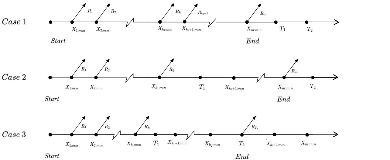
Figure 1: Schematic representation of IAT-II PCS

$$Case1: X_{1:m:n},X_{2:m:n},\dots,X_{m:m:n},\quad if\ X_{m:m:n}<T_{1}<T_{2},$$ (1)

$$Case2: X_{1:m:n},\dots,X_{k_{1}:m:n}\dots,X_{m:m:n},\quad if\ X_{k_{1}:m:n}<T_{1}<X_{m:m:n}<T_{2},$$ (2)

$$Case3: X_{1:m:n},\dots,X_{k_{1}:m:n}\dots,X_{k_{2}:m:n},\quad if\ X_{k_{1}:m:n}<T_{1}<X_{k_{2}:m:n}<T_{2},$$ (3)

The censoring scheme and the end position of the experiment in these three cases are as follows

$$Case1: R=(R_{1},R_{2},...,R_{m}),R_{m}=0,$$ (4)

$$Case2: R=(R_{1},R_{2},...,R_{k_{1}},0,...,0,R_{m}),R_{m}=n-m-\sum_{i=1}^{k_{1}}R_{i},$$ (5)

$$Case3: R=(R_{1},R_{2},...,R_{k_{1}},0,...,R_{k_{2}},R_{T_{2}}),R_{k_{2}}=0,R_{T_{2}}=n-k_{2}-\sum_{i=1}^{k_{1}}R_{i},$$ (6)

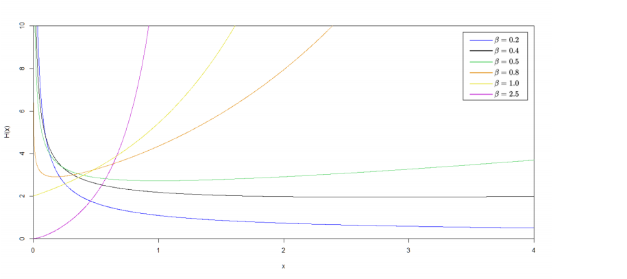
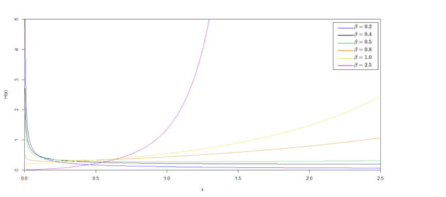
In real life, there are many hazard rate functions used to model real life data, the most popular failure rate functions are constant, increasing or decreasing failure rate functions. For example Weibull, gamma and exponentiated exponential, among others. But there are other different forms of the hazard function, such as unimodal, bathtub-shaped, increasing-decreasing-increasing, etc. These distribution models described above also do not fit reasonably non-monotonic hazard rates, especially bathtub shape hazard rates that are common in reliability and other fields. An example of a bathtub-shaped failure rate is that the failure rate of newly installed electronic equipment is relatively high, failures often occur, production performance drops to a minimum level for a short period of time, and then the equipment will stabilize after a few days or months of use, remaining at this level for several years, and then the equipment underwent various forms of overhaul or technical transformation to restore production performance. Yan et al. (2021) used the Burr-XII distribution in the IAT-II PC proposed in 2021, and its hazard rate function could not fit the data of the bathtub curve. In recent years, a number of probability distributions have been introduced to model the risk rate of having a bathtub shape, which can be found in the literature. In this paper, we mainly focus on a two-parameter bathtub distribution proposed by Chen (2000). the probability density function $(PDF)$ and cumulative distribution function $(CDF)$ of $X$ are given by

$$f(x;\alpha,\beta) =\alpha\beta x^{\beta-1}\exp\left[\alpha(1-e^{x^{\beta}})+x^{\beta}\right]\quad x>0,\alpha,\beta>0,$$ (7)

$$F(x;\alpha,\beta) =1-\exp\left[\alpha(1-e^{x^{\beta}})\right]\quad x>0,\alpha,\beta>0.$$ (8)

The reliability and the hazard rate functions hazard function of $X$ are as follows

$$S(x;\alpha,\beta) = \exp\left[\alpha(1-e^{x^{\beta}})\right]\quad x>0,\alpha,\beta>0,$$ (9)

$$H(x;\alpha,\beta) = \alpha\beta x^{\beta-1}e^{x^{\beta}}\quad x>0,\alpha,\beta>0,$$ (10)

where $\alpha$ and $\beta$ are the unknown scale and shape parameters, respectively, and when $\beta<1$, the hazard rate function is bathtub-shape.

Figure 2: Failure rate functions with $\alpha=2$.

Figure 3: Failure rate functions with $\alpha=0.2$.

The rest of this paper is organized as follows: In Section $2$, maximum likelihood estimate (MLE) on unknown parameters is derived and the approximate confidence intervals is proposed. In Section $3$, Bayesian estimation is performed with gamma prior, and Importance sampling and Metropolis-Hastings algorithm are used. Next, based on the Monte Carlo method, a large number of simulations are carried out for parameter estimations and interval estimations in Section $4$. A real data set has been used to evaluated the estimation methods in Section $2$ and $3$. Finally, in Section $6$, we put forward some concluding conclusions.

2 Model description and notation

Let $X=X_{1:m:n}^{R},X_{2:m:n}^{R},\dots,X_{k_{1}:m:n}^{R},\dots,X_{k_{2}:m:n}^{R},\dots,X_{m:m:n}^{R}$ is an IAT-II PC sample from a lifetime test of size $m$ from a sample of size $n$ , where lifetimes have Chen distribution with pdf,cdf as given by (7). With predetermined number of removal of units from experiment, say $R=(R_{1},R_{2},\dots,R_{k_{1}},\dots,R_{k_{2}},\dots,R_{m})$. The parameter $x_{i:m:n}^{R}$ (simplified as $x_{i}$ in later equation, $i=1,2,\dots,m$) is used to represent the observed values of IAT-II PC sample. on this basis, the corresponding likelihood function is given by

$$L=C\prod_{i=1}^{D_{2}}f(x_{i})\prod_{i=1}^{D_{1}}\left[\left(1-F(x_{i})\right)\right]^{R_{i}}\left(1-F(x_{B})\right)^{B},$$ (11)

where $D_{2}$, $D_{1}$, $B$, $C$ are shown in Table (1)

Table 1: Interpretation of $D_{2}$, $D_{1}$, $B$, $C$ in likelihood function

	$D_{2}$	$D_{1}$	$B$	C
Case1	$m$	$m$	$0$	$\prod\limits_{i=1}^{m}\left(n-i+1-\sum\limits_{s=1}^{i-1}R_{s}\right)$
Case2	$m$	$k_{1}$	$n-m-\sum\limits_{i=1}^{k_{1}}R_{i}$	$\prod\limits_{i=1}^{m}\left(n-i+1-\sum\limits_{s=1}^{k_{1}}R_{s}\right)\quad$
Case3	$k_{2}$	$k_{1}$	$n-k_{2}-\sum\limits_{i=1}^{k_{1}}R_{i}$	$\prod\limits_{i=1}^{m}\left(n-i+1-\sum\limits_{s=1}^{k_{1}}R_{s}\right)\quad$

Then, from (7), (11), The likelihood function of $\alpha$ and $\beta$ is given by

$$\begin{split}L(\alpha,\beta)=&C\left[\prod_{i=1}^{D_{2}}\alpha\beta x_{i}^{\beta-1}\exp\left(\alpha\left(1-e^{x_{i}^{\beta}}\right)+x_{i}^{\beta}\right)\right]\\ &\times\left[\prod_{i=1}^{D_{1}}\left[\exp\left(\alpha\left(1-e^{x_{i}^{\beta}}\right)\right)\right]^{R_{i}}\right]\left[\exp\left(\alpha\left(1-e^{x_{B}^{\beta}}\right)\right)\right]^{B}.\end{split}$$ (12)

Then, we propose several statistical inference methods.

2.1 Maximum likelihood estimation

We can write the natural logarithm of the likelihood function as follows

$$\begin{split}\ln L(\alpha,\beta)=&\ln C+D_{2}\ln\alpha+D_{2}\ln\beta+\sum_{i=1}^{D_{2}}(\beta-1)\ln x_{i}\\ &+\alpha(1-e^{x_{i}^{\beta}})+x_{i}^{\beta}+\sum_{i=1}^{D_{1}}R_{i}\alpha(1-e^{x_{i}^{\beta}})+B\alpha(1-e^{x_{B}^{\beta}}).\end{split}$$ (13)

The Maximum likelihood estimations of $\alpha$ and $\beta$ can be obtained by solving the following two equations

$$\frac{\partial\ln L(\alpha,\beta)}{\partial\alpha}= \frac{D_{2}}{\alpha}+\sum_{i=1}^{D_{2}}(1-e^{x_{i}^{\beta}})+\sum_{i=1}^{D_{1}}R_{i}(1-e^{x_{i}^{\beta}})+B(1-e^{x_{B}^{\beta}})=0,$$ (14)

$$\frac{\partial\ln L(\alpha,\beta)}{\partial\beta}= \frac{D_{2}}{\beta}+\sum_{i=1}^{D_{2}}\ln x_{i}+x_{i}^{\beta}\ln x_{i}$$

$$-\alpha\left(\sum_{i=1}^{D_{2}}e^{x_{i}^{\beta}}x_{i}^{\beta}\ln x_{i}+\sum_{i=1}^{D_{1}}R_{i}e^{x_{i}^{\beta}}x_{i}^{\beta}\ln x_{i}+Be^{x_{B}^{\beta}}x_{B}^{\beta}\ln x_{B}\right)=0.$$ (15)

From (14), the MLE of $\alpha$ can be obtained as follows

$$\hat{\alpha}=\frac{D2}{\nu(x_{i},\beta)},$$ (16)

where $\nu(x_{i},\beta)=\sum_{i=1}^{D_{2}}(e^{x_{i}^{\beta}}-1)+\sum_{i=1}^{D_{1}}R_{i}(e^{x_{i}^{\beta}}-1)+B(e^{x_{B}^{\beta}}-1)$. Now substitute equation (16) into equation (15), substituting $\hat{\alpha}$ for $\alpha$ to get the MLE estimate of $\beta$ as follows

$$\frac{D_{2}}{\beta}+\sum_{i=1}^{D_{2}}\ln x_{i}(1+x_{i}^{\beta})-\frac{D2}{\nu(x_{i},\beta)}\left(\sum_{i=1}^{D_{2}}\phi_{i}(x_{i},\beta)+\sum_{i=1}^{D_{1}}R_{i}\phi_{i}(x_{i},\beta)+B\phi_{B}(x_{B},\beta)\right)=0,$$ (17)

where $\phi_{i}(x_{i},\beta)=e^{x_{i}^{\beta}}x_{i}^{\beta}\ln x_{i}$. Equation (17) does not have a closed-form solution, so the MLE of $\beta$ can be obtained by numerical methods of the following nonlinear equations

$$g(\beta)=\left(-\frac{\sum_{i=1}^{D_{2}}\ln x_{i}(1+x_{i}^{\beta})}{D_{2}}+\frac{\sum_{i=1}^{D_{2}}\phi_{i}(x_{i},\beta)+\sum_{i=1}^{D_{1}}R_{i}\phi_{i}(x_{i},\beta)+B\phi_{B}(x_{B},\beta)}{\nu(x_{i},\beta)}\right)^{-1}.$$ (18)

The MLE of $\beta$ is denoted by $\hat{\beta}$, and the solution for $g(\beta)=\beta$ can be obtained by a simple iterative method

$$\beta^{(k+1)}=g(\beta^{(k)}),$$

here $\beta^{(k)}$ represents the $k$-$th$ iteration, and the iterative process stops when the difference between two consecutive solutions is less than a predetermined tolerance limit. When we obtain the MLE of $\beta$, the MLE of $\alpha$ can be obtained directly from equation (16).

2.2 Approximate Confidence Intervals

In this subsection, we further discuss the $(1-\gamma)\times 100\%$ approximate confidence intervals for the unknown parameters $\lambda=(\alpha,\beta)$ based on the asymptotic distribution of the MLE $\hat{\lambda}$ is $(\hat{\lambda}-\lambda)\to N_{2}(0,I^{-1}(\lambda))$ (see[Jerald. (1982)]). where $I^{-1}(\lambda)$ is defined as the inverse Fisher information matrix of the two unknown parameters.

The fisher information matrix $I(\lambda)$ is written as which elements are negatives of expected values of the second partial derivatives of the $\ln L(\alpha,\beta)$. The results are as follows

$$I(\lambda)=-E\begin{bmatrix}\frac{\partial^{2}\ln L(\alpha,\beta)}{\partial^{2}\alpha}&\frac{\partial^{2}\ln L(\alpha,\beta)}{\partial\alpha\partial\beta}\\ \frac{\partial^{2}\ln L(\alpha,\beta)}{\partial\beta\partial\alpha}&\frac{\partial^{2}\ln L(\alpha,\beta)}{\partial^{2}\beta}\end{bmatrix}.$$ (19)

In general, it can be shown that the asymptotic variance-covariance matrix of $MLE$ is inverting the fisher information matrix $I^{-1}(\lambda)$. The specific details are as follows

$$I^{-1}(\lambda)=\begin{bmatrix}-\frac{\partial^{2}\ln L(\alpha,\beta)}{\partial^{2}\alpha}&-\frac{\partial^{2}\ln L(\alpha,\beta)}{\partial\alpha\partial\beta}\\ -\frac{\partial^{2}\ln L(\alpha,\beta)}{\partial\beta\partial\alpha}&-\frac{\partial^{2}\ln L(\alpha,\beta)}{\partial^{2}\beta}\end{bmatrix}_{(\alpha,\beta)=(\hat{\alpha},\hat{\beta})}^{-1}=\begin{bmatrix}var(\hat{\alpha})&cov(\hat{\alpha},\hat{\beta})\\ cov(\hat{\beta},\hat{\alpha})&var(\hat{\beta})\end{bmatrix}.$$ (20)

From the log-likelihood function in (13) we can obtain the second derivatives of $\ln L(\alpha,\beta)$ as follow

$$\frac{\partial^{2}\ln L(\alpha,\beta)}{\partial^{2}\alpha} = -\frac{D_{2}}{\alpha^{2}},$$

$$\frac{\partial^{2}\ln L(\alpha,\beta)}{\partial^{2}\beta} = -\frac{D_{2}}{\beta^{2}}+\sum_{i=1}^{D_{2}}\ln^{2}x_{i}x_{i}^{\beta}-\alpha\left(\sum_{i=1}^{D_{2}}\phi_{i}\xi_{i}+\sum_{i=1}^{D_{1}}R_{i}\phi_{i}\xi_{i}+B\phi_{B}\xi_{B}\right),$$ (21)

$$\frac{\partial^{2}\ln L(\alpha,\beta)}{\partial\beta\partial\alpha} = \frac{\partial^{2}\ln L(\alpha,\beta)}{\partial\alpha\partial\beta\ }=-\left(\sum_{i=1}^{D_{2}}\phi_{i}+\sum_{i=1}^{D_{1}}R_{i}\phi_{i}+B\phi_{B}\right),$$

where $\xi_{i}=\ln x_{i}(1+x_{i}^{\beta})$, $\xi_{B}=\ln x_{B}(1+x_{B}^{\beta})$, $\frac{\partial\phi_{i}(x_{i},\beta)}{\partial\beta}=\exp(x_{i}^{\beta})x_{i}^{\beta}\ln x_{i}\xi_{i}$.

Therefore, we can obtain the $(1-\gamma)\times 100\%$ approximate confidence intervals for the parameters $\alpha$ and $\beta$ as follow

$$\left({\Large}\hat{\alpha}+Z_{\gamma/2}\sqrt{var(\alpha)},\ \hat{\alpha}+Z_{\gamma/2}\sqrt{var(\alpha)}\right),\quad\left({\Large}\hat{\beta}+Z_{\gamma/2}\sqrt{var(\beta)},\ \hat{\beta}+Z_{\gamma/2}\sqrt{var(\beta)}\right),$$ (22)

where $Z_{\gamma/2}$ is the upper $(\gamma/2)^{th}$ percentile point of a standard normal distribution.

3 Bayesian estimation

This section is devoted to obtain the Bayes estimators of the parameters $\alpha$ and $\beta$ of Chen distribution based on improved adaptive asymptotic type-II censored data. The Bayesian estimates are obtained using symmetric as well as asymmetric loss function such as squared error loss function(SEL), LINEX loss function(LL) and entropy loss(EL) function. We assume the parameters $\alpha$ and $\beta$ independent and have gamma prior distributions with the following prior distribution. $G(a,b)$ and $G(c,d)$ distribution with PDFs respectively as

$$\pi_{1}(\alpha;a,b)=\frac{b^{a}}{\Gamma(a)}\alpha^{a-1}e^{-b\alpha},\quad\alpha>0,a,b>0,$$

$$\pi_{2}(\beta;c,d)=\frac{d^{c}}{\Gamma(c)}\beta^{c-1}e^{-d\beta},\quad\beta>0,c,d>0.$$

Therefore, the joint prior distribution of $\alpha$ and $\beta$ is given by

$$\pi(\alpha,\beta)\propto\alpha^{a-1}\beta^{c-1}e^{-(b\alpha+d\beta)}\quad\alpha,\beta>0,a,b,c,d>0.$$ (23)

Subsequently, the joint posterior distribution of $\alpha$ and $\beta$ becomes

$$\pi(\alpha,\beta\mid X)=\frac{L(\alpha,\beta X)\pi(\alpha,\beta)}{\int_{0}^{\infty}\int_{0}^{\infty}L(\alpha,\beta X)\pi(\alpha,\beta)\rm d\alpha\rm d\beta}.$$

Given $\alpha$, $\beta$, directly calculate the joint posterior distribution $\pi(\alpha,\beta\mid X)$ as follow

$$\begin{aligned} \pi(\alpha,\beta\mid X)\propto&\alpha^{D_{2}+a-1}\exp\left[-\alpha\left(b-\sum_{i=1}^{D_{2}}\left(1-e^{x_{i}^{\beta}}\right)-\sum_{i=1}^{D_{1}}R_{i}\left(1-e^{x_{i}^{\beta}}\right)\right.\right.\\ &\left.\left.-B\left(1-e^{x_{B}^{\beta}}\right)\right)\right]\times\beta^{D_{2}+c-1}\exp\left[-\beta\left(d-\sum_{i=1}^{D_{2}}logx_{i}\right)\right]\exp\left(\sum_{i=1}^{D_{2}}x_{i}^{\beta}\right).\end{aligned}$$ (24)

Under the square error loss function (SEL), the Bayes estimate for any parameter $\mu$ is given by

$$\hat{d}_{SEL}=E(\eta\mid\mu).$$ (25)

For LINEX loss function(LL), the Bayes estimate for any parameter $u$ is given by

$$\hat{d}_{LL}=-\frac{1}{g}\ln E_{\eta}(e^{-g\eta}\mid\mu).$$ (26)

For entropy loss function(EL), the Bayesian estimates obtained by minimizing the risk function are

$$\hat{d}_{EL}=\left[E_{\eta}({\eta^{-q}}\mid\mu)\right]^{-\frac{1}{q}}.$$ (27)

Where $g$ and $q$ are known constants, $\eta$ represents any one of the unknown parameters. Obviously, (25) (26) (27) cannot get an explicit solution. Therefore, the Markov chain Carlo method(MCMC) is used to generate samples from the posterior density function and in turn to compute the Bayesian estimation of the unknown parameters. The following two technique are introduced to calculate bayes estimation.

3.1 Metropolis-Hastings algorithm with Gibbs sampling

The Metropolis-Hastings (M-H) algorithm as a general Markov chain Monte Carlo (MCMC) method be introduced by Metropolis et al. (1953) and then Hastings (1970) extended the M-H algorithm. Gibbs sampling method is a special case of the MCMC method. It can be used to generated a sequence of sampling from the full conditional probability distributions of random variables. Gibbs sampling requires that the joint posterior distribution of each parameter be decomposed into full conditional distribution and then sampling from them. We can apply the Gibbs sampling procedure to generate a sample from (24), and then compute the Bayesian estimation.

Therefore, the posterior conditional density function of $\alpha$ and $\beta$ can be obtained as

$$\pi(\alpha\mid\beta,x)\propto\alpha^{D_{2}+a-1}\exp\left[-\alpha\left[b-\sum_{i=1}^{D_{2}}(1-e^{x_{i}^{\beta}})-\sum_{i=1}^{D_{1}}R_{i}(1-e^{x_{i}^{\beta}})-B(1-e^{x_{B}^{\beta}})\right]\right],$$ (28)

$$\ \pi(\beta\mid\alpha,x)\propto\beta^{D_{2}+c-1}\exp\left[-\beta\left(d-\sum_{i=1}^{D_{2}}\ln x_{i}\right)\right]\exp\left(\sum_{i=1}^{D_{2}}x_{i}^{\beta}\right),$$ (29)

here, we use the M-H algorithm with Gibbs sampling to generate samples from (28) and (29). The M-H algorithm is performed for Bayesian estimates.

Algorithm 1 Metropolis-Hastings algorithm

0:  Bayesian estimators of the parameters $\alpha$ and $\beta$ under different loss function with Metropolis-Hastings technique.

0:   Step1 : The initial value of the given parameters is $\eta^{(0)}=(\alpha^{(0)},\beta^{(0)})$.Step2 : Use Metropolis-Hasting algorithm to generate $\alpha^{(0)}$ from(28) and $\beta^{(0)}$ from (29) as the Gibbs sampling iteration values. $q(\beta)=N(\hat{\beta})$. Take the normal distribution as the proposal distribution. Repeat $N$ times, then we get $\eta^{(h)}=(\alpha^{(h)},\beta^{(h)}),\quad h=1,2,...,N$.Step3 : Take the first $M$ results as a burn-in phase. Under different loss function, Bayesian estimations are

$$\hat{d}_{SEL} = \frac{1}{N-M}\sum_{h=M+1}^{N}\eta^{(h)},$$

$$\hat{d}_{LL} = -\frac{1}{g}\ln\left(\frac{1}{N-M}\sum_{h=M+1}^{N}e^{g\eta^{{\scriptsize(}h{\scriptsize)}}}\right),$$

$$\hat{d}_{EL} = \left[\frac{1}{N-M}\sum_{h=M+1}^{N}\left(\eta^{{\scriptsize(}h{\scriptsize)}}\right)^{-q}\right]^{-\frac{1}{q}}.$$

Step4 : Get the results in step2. Sort in ascending order as $\left(\eta_{(1)},\eta_{(2)},...,\eta_{(N)}\right)$.

3.2 Importance sampling technique

The importance sampling method can be used to compute the approximate results of (25), (26) and (27), so as to obtain the Bayesian estimations. From (24), we have

$$\pi(\alpha,\beta\mid X)\propto g(\alpha\mid\beta,x)g(\beta\mid x)\omega(\alpha,\beta),$$ (30)

where

$$g(\alpha\mid\beta,x) \propto \alpha^{D_{2}+a-1}\exp\left[-\alpha\left[b+\sum_{i=1}^{D_{1}}R_{i}\left(e^{x_{i}^{\beta}}-1\right)+B\left(e^{x_{B}^{\beta}}-1\right)\right]\right],$$ (31)

$$g(\beta\mid x) \propto \beta^{D_{2}+c-1}\exp\left[-\beta\left(d-\sum_{i=1}^{D_{2}}logx_{i}\right)\right],$$ (32)

$$\omega(\alpha,\beta) \propto \frac{\exp\left[\sum_{i=1}^{D_{2}}\alpha\left(1-e^{x_{i}^{\beta}}\right)+\sum_{i=1}^{D_{2}}x_{i}^{\beta}\right]}{\left[b+\nu\left(x_{i},\beta\right)\right]^{D_{2}+a}},\ \ \ \ \$$ (33)

where $\nu(x_{i},\beta)=\sum_{i=1}^{D_{2}}(e^{x_{i}^{\beta}}-1)+\sum_{i=1}^{D_{1}}R_{i}(e^{x_{i}^{\beta}}-1)+B(e^{x_{B}^{\beta}}-1)$. Note that the distribution of $g(\alpha\mid\beta,x)$ follows Gamma distribution with parameters$(D_{2}+a-1)$ and $(b-\sum_{i=1}^{D_{2}}(1-e^{x_{i}^{\beta}})-\sum_{i=1}^{D_{1}}R_{i}(1-e^{x_{i}^{\beta}})-B(1-e^{x_{B}^{\beta}}))$. The distribution of $g(\beta\mid x)$ follow Gamma distribution with parameters $(D_{2}+c-1)$ and $(d-\sum_{i=1}^{D_{2}}\log x_{i})$. Therefore, one can easily generate samples from the distribution of $\alpha$ and $\beta$, respectively. Then by the importance sampling method, the Bayesian estimation of $\alpha$ and $\beta$ under the squared error loss function are obtained as

$$\hat{\alpha}_{SEL}=\frac{\sum_{i=1}^{N_{2}}\alpha^{(i)}\omega^{(i)}}{\sum_{i=1}^{N_{2}}\omega^{(i)}},$$ (34)

and

$$\hat{\beta}_{SEL}=\frac{\sum_{i=1}^{N_{2}}\beta^{(i)}\omega^{(i)}}{\sum_{i=1}^{N_{2}}\omega^{(i)}}.$$ (35)

Similarly, the Bayesian estimation of $\alpha$ and $\beta$ under the LINEX loss function are obtained as

$$\hat{\alpha}_{LL}=-\frac{1}{g}\ln\left[\frac{\sum_{i=1}^{N_{2}}e^{-g\alpha^{(i)}}\omega^{(i)}}{\sum_{i=1}^{N_{2}}\omega^{(i)}}\right],$$ (36)

and

$$\hat{\beta}_{LL}=-\frac{1}{g}\ln\left[\frac{\sum_{i=1}^{N_{2}}e^{-g\beta^{(i)}}\omega^{(i)}}{\sum_{i=1}^{N_{2}}\omega^{(i)}}\right].$$ (37)

Again the Bayesian estimation of $\alpha$ and $\beta$ under the entropy loss function are obtained as

$$\hat{\alpha}_{EL}=\left[\frac{\sum_{i=1}^{N_{2}}(\alpha^{{\scriptsize(}i{\scriptsize)}})^{-q}\omega^{(i)}}{\sum_{i=1}^{N_{2}}\omega^{(i)}}\right]^{-\frac{1}{q}},$$ (38)

and

$$\hat{\beta}_{EL}=\left[\frac{\sum_{i=1}^{N_{2}}(\beta^{{\scriptsize(}i{\scriptsize)}})^{-q}\omega^{(i)}}{\sum_{i=1}^{N_{2}}\omega^{(i)}}\right]^{-\frac{1}{q}}.$$ (39)

The procedure of importance sampling is given as follows

Algorithm 2 Importance sampling algorithm

0:  Bayesian estimators of the parameters $\alpha$ and $\beta$ under different loss function with importance sampling technique.

0:   Step1: Generate $\beta^{(1)}$ from $g(\beta\mid x)$.Step2: Generate $\alpha^{(1)}$ from $g(\alpha\mid\beta,x)$.Step3: Calculate $\omega^{(1)}(\beta^{(1)})$ and $\theta^{(1)}=\theta(\alpha^{(1)},\beta^{(1)})$.Step4: Respect the above process $N_{2}$ times and obtain $\left(\omega^{(1)},\omega^{(2)},...,\omega^{(N_{2})}\right)$ and $\left(\theta^{(1)},\theta^{(2)},...,\theta^{(N_{2})}\right)$.Step5: Calculate the Bayesian estimators of the parameters $\alpha$ and $\beta$ under different loss function.

4 Simulation experiments

In this section, the simulation study is carried out Monte Carlo simulation to evaluate the performance of the proposed methods. The Biases and mean square errors(MSE) of the MLE and Bayesian estimates for $\alpha$ and $\beta$ are evaluated under the IAT-II PCS and and in $R$ program. The Bayesian estimates are computed by using Importance sampling and M-H technique. Under different combination of $(n,m)$ and different censoring schemes $(T_{1},T_{2},R_{1},R_{2},\cdots,R_{m})$. the point and interval estimation results are assessed on the basis of mean Bias and MSE respectively.

All the estimates are to compute arbitrary the unknown parameter values $\alpha=0.2$ and $\beta=0.5)$. Accordingly hyperparameters in gamma prior are assigned as $a=2$, $b=2,$ and $c=2$, $d=2$. Here we consider four different censoring schemes, namely:

Scheme1 $$: R_{m}=n-m,R_{i}=0\ \ \textup{for}\ i\neq m.$$

Scheme2 $$: R_{1}=n-m,R_{i}=0\ \ \textup{for}\ i\neq 1.$$

Scheme3 $$: R_{\frac{m+1}{2}}=n-m,R_{i}=0\ \ \textup{for}\ i\neq\frac{m+1}{2};\ \textup{if}\ m\ \textup{is}\ \textup{odd},\ \textup{and}$$

$$R_{\frac{m}{2}}=n-m,R_{i}=0\ \ \textup{for}\ i\neq\frac{m}{2},\ \textup{if}\ m\ \textup{is}\ \textup{even}.$$

Scheme4 $$: R_{i}=\frac{n-m}{m},\quad i=1,2,\cdots,m.$$

In our study, two expected time on test $(T_{1},T_{2})$ are (0.4,4) and (1,7). We consider three different values of $(n,m)$, namely (15,5), (20,10) and (30,15). For evaluating Bayes estimators under LINEX loss function, we take $g=1$ and for entropy loss function, we take $q=1$. Based on the simulation study we have the following conclusion.

From the simulate results in Table 2 and 3, one can observe following conclusions for MLE. From these Tables the following conclusion are made:

1. The estimation of MLE is evaluated by Bias and MSE, among which MSE is better than Bias.

2. In most cases, for different censoring schemes, Scheme 4 is uniform censoring scheme and others are non-uniform schemes. It can be seen from the table that the estimation effect of uniform censoring scheme is better than that of other non-uniform censoring schemes.

3. Compared with Table 2 and Table 3, in most cases, when the time threshold becomes larger, the Bias and MSE of related MLE becomes larger, the estimation effect of $(T_{1},T_{2})=(1,7)$ is poor. Therefore, it is essential to set a reasonable time threshold in the experiment.

Table 2: Bias and MSE of the MLE $\hat{\alpha}$ and $\hat{\beta}$ for different choices of $n,m$ and $T_{1}=0.4,T_{2}=4$.

				$\hat{\alpha}$			$\hat{\beta}$
n,m	scheme	$\alpha$	$\beta$	Bias	MSE		Bias	MSE
	I	0.2	0.5	-0.18276	0.03340		0.11049	0.01221
	II	0.2	0.5	-0.06933	0.00481		-0.24902	0.06201
15,5	III	0.2	0.5	-0.19048	0.03628		0.17394	0.03026
	IV	0.2	0.5	-0.03561	0.00127		-0.01553	0.00024
	I	0.2	0.5	-0.08918	0.00795		0.25224	0.06362
	II	0.2	0.5	0.09200	0.00846		-0.23686	0.05610
20,10	III	0.2	0.5	0.06425	0.00413		-0.14137	0.01998
	IV	0.2	0.5	-0.05793	0.00336		0.11998	0.01440
	I	0.2	0.5	-0.17254	0.02977		0.41297	0.17055
	II	0.2	0.5	-0.11648	0.01357		-0.35441	0.12561
30,15	III	0.2	0.5	-0.10793	0.01165		-0.08880	0.00789
	IV	0.2	0.5	0.02276	0.00052		-0.21521	0.04632

Table 3: Bias and MSE of the MLE $\hat{\alpha}$ and $\hat{\beta}$ for different choices of $n,m$ and $T_{1}=1,T_{2}=7$.

				$\hat{\alpha}$			$\hat{\beta}$
n,m	scheme	$\alpha$	$\beta$	Bias	MSE		Bias	MSE
	I	0.2	0.5	-0.09838	0.00968		-0.03055	0.00093
	II	0.2	0.5	-0.11620	0.01350		-0.34789	0.12103
15,5	III	0.2	0.5	-0.08268	0.00684		-0.34844	0.12141
	IV	0.2	0.5	-0.11235	0.01262		0.21203	0.04496
	I	0.2	0.5	-0.11840	0.01402		0.18201	0.03313
	II	0.2	0.5	0.12462	0.01553		-0.22917	0.05252
20,10	III	0.2	0.5	-0.11064	0.01224		0.24352	0.05930
	IV	0.2	0.5	-0.12914	0.01668		0.31077	0.09658
	I	0.2	0.5	-0.11563	0.01337		0.19582	0.03834
	II	0.2	0.5	-0.11043	0.01219		0.23403	0.05477
30,15	III	0.2	0.5	0.07763	0.00603		-0.20020	0.04008
	IV	0.2	0.5	-0.08184	0.00670		0.16316	0.02662

Table 4 and 5 present the coverage probability and average length of two-side $95.5\%$ confidence intervals of parameters constructed by maximum likelihood method (using fisher observation information matrix). From these Tables the following conclusion are made:

1. The truth value of $\alpha=0.2$ and $\beta=0.5$ is in the middle of the each interval and can be well covered.

2. The asymptotic confidence interval of $\beta$ obtained by fisher observation information matrix, in most case, the average length of the interval is getting longer when the time threshold increase. Meanwhile, different censoring schemes $R$ had no significant effect on the $\alpha$ and $\beta$ results of interval estimation.

3. The average length of the interval about $\alpha$ is significantly different under the two time thresholds $(0.4,4)$ and $(1,7)$.

4. The asymptotic confidence interval of $\alpha$, in most case, are more ideal than that of $\beta$.

Table 4: Interval estimations,and Average Length(AL) for different choices of $n,m$ and $T_{1}=0.4,T_{2}=4$.

n,m	scheme	$\alpha$	$\beta$	$\alpha-AL$	$\beta-AL$
	I	(0.00129,0.58393)	(0.48694,1.71175)	0.58264	1.22482
	II	(0.02411,0.28934)	(0.04585,0.63700)	0.26523	0.59115
15,5	III	(0.02096,0.40454)	(0.11858,1.42586)	0.38358	1.30727
	IV	(0.06947,0.71424)	(0.09405,0.86234)	0.64476	0.76829
	I	(0.01640,0.70959)	(0.17385,0.90605)	0.57258	0.73220
	II	(0.13701,0.53979)	(0.01334,0.04607)	0.38361	0.03273
20,10	III	(0.13223,0.75290)	(0.14972,0.85257)	0.62068	0.70285
	IV	(0.10312,0.54511)	(0.14693,0.65170)	0.44199	0.50477
	I	(0.03949,0.31102)	(0.45257,1.11968)	0.27154	0.66710
	II	(0.15002,0.56836)	(0.11233,0.51236)	0.41834	0.40002
30,15	III	(0.12563,0.55586)	(0.16401,0.78419)	0.43023	0.62018
	IV	(0.06050,0.33362)	(0.36250,1.06036)	0.27311	0.69786

Table 5: Interval estimations,and Average Length(AL) for different choices of $n,m$ and $T_{1}=1,T_{2}=7$.

n,m	scheme	$\alpha$	$\beta$	$\alpha-AL$	$\beta-AL$
	I	(0.02227,0.46365)	(0.17421,1.26507)	0.44138	1.09087
	II	(0.02410,0.29141)	(0.04789,0.66570)	0.26731	0.61781
15,5	III	(0.02988,0.46066)	(0.04098,0.80587)	0.43079	0.76489
	IV	(0.02385,0.32205)	(0.31173,2.04524)	0.29820	1.73351
	I	(0.02728,0.73341)	(0.09402,0.61997)	0.58973	0.52595
	II	(0.13713,0.76841)	(0.08804,0.65271)	0.63127	0.56467
20,10	III	(0.02880,0.27724)	(0.46691,1.07021)	0.24844	0.60330
	IV	(0.01690,0.29710)	(0.47157,1.23919)	0.28020	0.76762
	I	(0.03392,0.20986)	(0.48876,0.96220)	0.17594	0.47344
	II	(0.04174,0.33184)	(0.38175,1.41139)	0.29011	1.02963
30,15	III	(0.14169,0.54398)	(0.15428,0.58258)	0.40229	0.40229
	IV	(0.05112,0.27315)	(0.41602,1.05710)	0.22203	0.64107

Table 6, 7, 8, 9 present the Bias and MSE of Bayesian estimation of $\alpha$ and $\beta$ by importance sampling technique under squared error loss function, LINEX loss function and entropy loss function. Table 10, 11, 12, 13 present the Bias and MSE of Bayesian estimation by Metropolis-Hasting technique of $\alpha$ and $\beta$. From these Tables the following conclusion are made:

1. For the tables, we can also see that Bias and MSE of Bayes estimators of $\alpha$ and $\beta$ are smaller than Bias and MSE of corresponding MLE.

2. From Table 6, 8 and Table 7, 9, in most cases, one can see that Bayesian estimators of $\alpha$ and $\beta$ by importance sampling technique under squared error loss function possess minimum Bias and MSE. When the time threshold increase, under entropy loss function also possess minimum Bias and MSE. From Table 10 and Table 12, one can see Bayesian estimators of $\alpha$ by M-H technique under squared error loss function possess minimum Bias and MSE. From Table 11 Bayesian estimators of $\beta$ by M-H technique under LINEX loss function possess minimum Bias and MSE, when the time threshold is $(T_{1},T_{2})=(0.4,4)$ and Table 13, Bayesian estimators of $\beta$ by M-H technique under LINEX loss function and entropy loss function possess minimum Bias and MSE, when the time threshold is $(T_{1},T_{2})=(1,7)$.

3. The Bias and MSE of Bayesian estimation using M-H technique, in most case, are smaller than that using importance sampling.

Table 6: Bias and MSE of the Bayesian estimates by importance sampling technique of $\hat{\alpha}$ under squared error loss function $\hat{\alpha}_{SEL}$, LINEX loss function $\hat{\alpha}_{LL}$, and entropy loss function $\hat{\alpha}_{EL}$, for different choices of $n,m,\alpha,\beta$ and $T_{1}=0.4,T_{2}=4$.

				$\hat{\alpha}_{SEL}$			$\hat{\alpha}_{LL}$			$\hat{\alpha}_{EL}$
n,m	sc	alpha	beta	Bias	MSE		Bias	MSE		Bias	MSE
	I	0.2	0.5	-0.05442	0.00296		-0.05454	0.00297		-0.05571	0.00310
	II	0.2	0.5	0.00409	0.00002		0.00236	0.00001		-0.01083	0.00012
15,5	III	0.2	0.5	-0.03628	0.00132		-0.03630	0.00132		-0.03644	0.00133
	IV	0.2	0.5	-0.08628	0.00744		-0.08746	0.00765		-0.10018	0.01004
	I	0.2	0.5	-0.05352	0.00286		-0.05365	0.00288		-0.05504	0.00303
	II	0.2	0.5	-0.07435	0.00553		-0.07471	0.00558		-0.07949	0.00632
20,10	III	0.2	0.5	0.01078	0.00012		0.01070	0.00011		0.01009	0.00010
	IV	0.2	0.5	0.01141	0.00013		0.00952	0.00009		-0.00244	0.00001
	I	0.2	0.5	-0.10540	0.01111		-0.10750	0.01156		-0.13787	0.01901
	II	0.2	0.5	0.05013	0.00251		0.04831	0.00233		0.03676	0.00135
30,15	III	0.2	0.5	-0.02612	0.00068		-0.02675	0.00072		-0.03156	0.00100
	IV	0.2	0.5	0.01169	0.00014		0.01142	0.00013		0.00932	0.00009

Table 7: Bias and MSE of the Bayesian estimates by importance sampling technique of $\hat{\beta}$ under squared error loss function $\hat{\beta}_{SEL}$ LINEX loss function $\hat{\beta}_{LL}$ and entropy loss function $\hat{\beta}_{EL}$ for different choices of $n,m,\alpha,\beta$ and $T_{1}=0.4,T_{2}=4$.

				$\hat{\beta}_{SEL}$			$\hat{\beta}_{LL}$			$\hat{\beta}_{EL}$
n,m	sc	$\alpha$	$\beta$	Bias	MSE		Bias	MSE		Bias	MSE
	I	0.2	0.5	0.06578	0.00433		0.06322	0.00400		0.05649	0.00319
	II	0.2	0.5	0.11644	0.01356		0.10269	0.01055		0.04396	0.00193
15,5	III	0.2	0.5	0.09152	0.00838		0.09152	0.00838		0.09152	0.00838
	IV	0.2	0.5	0.07352	0.00541		0.06354	0.00404		0.04380	0.00192
	I	0.2	0.5	-0.04531	0.00205		-0.04584	0.00210		-0.04785	0.00229
	II	0.2	0.5	0.15521	0.02409		0.12921	0.01670		0.01849	0.00034
20,10	III	0.2	0.5	-0.00909	0.00008		-0.00917	0.00008		-0.00943	0.00009
	IV	0.2	0.5	-0.01205	0.00015		-0.01630	0.00027		-0.03579	0.00128
	I	0.2	0.5	0.21632	0.04679		0.21328	0.04549		0.20346	0.04140
	II	0.2	0.5	0.25439	0.06471		0.24590	0.06047		0.21985	0.04834
30,15	III	0.2	0.5	-0.07071	0.00500		-0.07143	0.00510		-0.07462	0.00557
	IV	0.2	0.5	0.15959	0.02547		0.15892	0.02526		0.15735	0.02476

Table 8: Bias and MSE of the Bayesian estimates by importance sampling technique of $\hat{\alpha}$ under squared error loss function $\hat{\alpha_{SEL}}$, LINEX loss function $\hat{\alpha_{LL}}$, and entropy loss function $\hat{\alpha_{EL}}$, for different choices of $n,m,\alpha,\beta$ and $T_{1}=1,T_{2}=7$.

				$\hat{\alpha_{SEL}}$			$\hat{\alpha_{LL}}$			$\hat{\alpha_{EL}}$
n,m	sc	$\alpha$	$\beta$	Bias	MSE		Bias	MSE		Bias	MSE
	I	0.2	0.5	0.02854	0.00081		0.02854	0.00081		0.02845	0.00081
	II	0.2	0.5	-0.05099	0.00260		-0.05099	0.00260		-0.05576	0.00311
15,5	III	0.2	0.5	0.06638	0.00441		0.06638	0.00441		0.06353	0.00404
	IV	0.2	0.5	0.04207	0.00177		0.04207	0.00177		0.04180	0.00175
	I	0.2	0.5	-0.00651	0.00004		-0.00651	0.00004		-0.01564	0.00024
	II	0.2	0.5	0.05089	0.00259		0.05089	0.00259		0.04696	0.00220
20,10	III	0.2	0.5	-0.09754	0.00951		-0.09754	0.00951		-0.09998	0.01000
	IV	0.2	0.5	0.09069	0.00823		0.09069	0.00823		0.08205	0.00673
	I	0.2	0.5	-0.05424	0.00294		-0.05424	0.00294		-0.05457	0.00298
	II	0.2	0.5	-0.06160	0.00379		-0.06160	0.00379		-0.06420	0.00412
30,15	III	0.2	0.5	-0.04417	0.00195		-0.04417	0.00195		-0.04914	0.00241
	IV	0.2	0.5	0.00413	0.00002		0.00413	0.00002		0.00167	0.00000

Table 9: Bias and MSE of the Bayesian estimates by importance sampling technique of $\hat{\beta}$ under squared error loss function $\hat{\beta}_{SEL}$ LINEX loss function $\hat{\beta}_{LL}$ and entropy loss function $\hat{\beta}_{EL}$ for different choices of $n,m,\alpha,\beta$ and $T_{1}=1,T_{2}=7$.

				$\hat{\beta}_{SEL}$			$\hat{\beta}_{LL}$			$\hat{\beta}_{EL}$
n,m	sc	$\alpha$	$\beta$	Bias	MSE		Bias	MSE		Bias	MSE
	I	0.2	0.5	-0.01712	0.00029		-0.01712	0.00029		-0.01714	0.00029
	II	0.2	0.5	-0.15450	0.02387		-0.15542	0.02416		-0.16039	0.02572
15,5	III	0.2	0.5	-0.10080	0.01016		-0.30124	0.09074		-0.30434	0.09262
	IV	0.2	0.5	0.06374	0.00406		-0.13645	0.01862		-0.13695	0.01876
	I	0.2	0.5	0.08405	0.00706		0.07961	0.00634		0.04465	0.00199
	II	0.2	0.5	0.02863	0.00082		0.02693	0.00073		0.01339	0.00018
20,10	III	0.2	0.5	0.03779	0.00143		0.03532	0.00125		0.02682	0.00072
	IV	0.2	0.5	-0.11941	0.01426		-0.12013	0.01443		-0.12269	0.01505
	I	0.2	0.5	0.07355	0.00541		0.07316	0.00535		0.07221	0.00521
	II	0.2	0.5	0.04997	0.00250		0.04939	0.00244		0.04749	0.00226
30,15	III	0.2	0.5	-0.06077	0.00369		-0.06093	0.00371		-0.06154	0.00379
	IV	0.2	0.5	0.06078	0.00369		0.06014	0.00362		0.05806	0.00337

Table 10: Bias and MSE of the Bayesian estimates by M-H technique of $\hat{\alpha}$ under squared error loss function $\hat{\alpha}_{SEL}$, LINEX loss function $\hat{\alpha}_{LL}$, and entropy loss function $\hat{\alpha}_{EL}$, for different choices of $n,m,\alpha,\beta$ and $T_{1}=0.4,T_{2}=4$.

				$\hat{\alpha}_{SEL}$			$\hat{\alpha}_{LL}$			$\hat{\alpha}_{EL}$
n,m	sc	$\alpha$	$\beta$	Bias	MSE		Bias	MSE		Bias	MSE
	I	0.2	0.5	-0.03289	0.00108		-0.05811	0.00338		-0.16499	0.02722
	II	0.2	0.5	0.02562	0.00066		0.01058	0.00011		-0.00766	0.00006
15,5	III	0.2	0.5	-0.03411	0.00116		-0.07142	0.00510		-0.13038	0.01700
	IV	0.2	0.5	0.05093	0.00259		0.01892	0.00036		-0.03241	0.00105
	I	0.2	0.5	-0.02719	0.00074		-0.07549	0.00570		-0.16503	0.02723
	II	0.2	0.5	-0.00444	0.00002		-0.02316	0.00054		-0.03929	0.00154
20,10	III	0.2	0.5	0.00170	0.00000		-0.03327	0.00111		-0.07890	0.00622
	IV	0.2	0.5	-0.01749	0.00031		-0.04216	0.00178		-0.14863	0.02209
	I	0.2	0.5	0.08353	0.00698		0.06098	0.00372		-0.03633	0.00132
	II	0.2	0.5	-0.03041	0.00092		-0.05154	0.00266		-0.11496	0.01322
30,15	III	0.2	0.5	0.06115	0.00374		0.04258	0.00181		0.01858	0.00035
	IV	0.2	0.5	0.00978	0.00010		-0.01915	0.00037		-0.12970	0.01682

Table 11: Bias and MSE of the Bayesian estimation by Metropolis-Hasting technique of $\hat{\beta}$ under squared error loss function $\hat{\beta}_{SEL}$ LINEX loss function $\hat{\beta}_{LL}$ and entropy loss function $\hat{\beta}_{EL}$ for different choices of $n,m,\alpha,\beta$ and $T_{1}=0.4,T_{2}=4$.

				$\hat{\beta}_{SEL}$			$\hat{\beta}_{LL}$			$\hat{\beta}_{EL}$
n,m	sc	$\alpha$	$\beta$	Bias	MSE		Bias	MSE		Bias	MSE
	I	0.2	0.5	-0.02572	0.00066		-0.04132	0.00171		-0.03905	0.00153
	II	0.2	0.5	0.06254	0.00391		0.04549	0.00207		0.04602	0.00212
15,5	III	0.2	0.5	-0.02232	0.00050		-0.05789	0.00335		-0.13166	0.01734
	IV	0.2	0.5	-0.02203	0.00049		-0.03712	0.00138		-0.03318	0.00110
	I	0.2	0.5	0.06556	0.00430		0.04950	0.00245		0.05266	0.00277
	II	0.2	0.5	0.04908	0.00241		0.03299	0.00109		0.03581	0.00128
20,10	III	0.2	0.5	0.04123	0.00170		0.02461	0.00061		0.02561	0.00066
	IV	0.2	0.5	0.05221	0.00273		0.03508	0.00123		0.03523	0.00124
	I	0.2	0.5	0.27074	0.07330		0.20603	0.04245		-0.01829	0.00033
	II	0.2	0.5	0.20663	0.04269		0.14835	0.02201		-0.26525	0.07036
30,15	III	0.2	0.5	-0.00897	0.00008		-0.06634	0.00440		-0.33857	0.11463
	IV	0.2	0.5	0.09338	0.00872		0.04952	0.00245		-0.20184	0.04074

Table 12: Bias and MSE of the Bayesian estimation by Metropolis-Hasting technique of $\hat{\alpha}$ under squared error loss function $\hat{\alpha}_{SEL}$, LINEX loss function $\hat{\alpha}_{LL}$, and entropy loss function $\hat{\alpha}_{EL}$, for different choices of $n,m,\alpha,\beta$ and $T_{1}=1,T_{2}=7$.

				$\hat{\alpha}_{SEL}$			$\hat{\alpha}_{LL}$			$\hat{\alpha}_{EL}$
n,m	sc	$\alpha$	$\beta$	Bias	MSE		Bias	MSE		Bias	MSE
	I	0.2	0.5	0.00518	0.00003		-0.01761	0.00031		-0.16221	0.02631
	II	0.2	0.5	0.05806	0.00337		0.04225	0.00178		0.02617	0.00068
15,5	III	0.2	0.5	-0.00693	0.00005		-0.03054	0.00093		-0.16305	0.02658
	IV	0.2	0.5	0.05205	0.00271		0.03126	0.00098		-0.01381	0.00019
	I	0.2	0.5	0.05050	0.00255		0.02748	0.00075		-0.05710	0.00326
	II	0.2	0.5	-0.04886	0.00239		-0.06539	0.00428		-0.08724	0.00761
20,10	III	0.2	0.5	0.00867	0.00008		-0.02407	0.00058		-0.07979	0.00637
	IV	0.2	0.5	0.02826	0.00080		-0.01598	0.00026		-0.12982	0.01685
	I	0.2	0.5	0.04949	0.00245		0.02357	0.00056		-0.12603	0.01588
	II	0.2	0.5	-0.02273	0.00052		-0.03918	0.00154		-0.06612	0.00437
30,15	III	0.2	0.5	0.03766	0.00142		0.01636	0.00027		-0.05739	0.00329
	IV	0.2	0.5	0.04199	0.00176		0.01822	0.00033		-0.08413	0.00708

Table 13: Bias and MSE of the Bayesian estimation by Metropolis-Hasting technique of $\hat{\beta}$ under squared error loss function $\hat{\beta}_{SEL}$ LINEX loss function $\hat{\beta}_{LL}$ and entropy loss function $\hat{\beta}_{EL}$ for different choices of $n,m,\alpha,\beta$ and $T_{1}=1,T_{2}=7$.

				$\hat{\beta}_{SEL}$			$\hat{\beta}_{LL}$			$\hat{\beta}_{EL}$
n,m	sc	$\alpha$	$\beta$	Bias	MSE		Bias	MSE		Bias	MSE
	I	0.2	0.5	-0.01451	0.00021		-0.04061	0.00165		-0.13918	0.01937
	II	0.2	0.5	-0.12429	-0.12429		-0.14812	0.02194		-0.18092	0.03273
15,5	III	0.2	0.5	-0.20364	0.04147		-0.23067	0.05321		-0.29499	0.08702
	IV	0.2	0.5	0.04736	0.00224		-0.00273	0.00001		-0.18747	0.03514
	I	0.2	0.5	0.13877	0.01926		0.09580	0.00918		-0.04724	0.00223
	II	0.2	0.5	0.05261	0.00277		0.03182	0.00101		0.02369	0.00056
20,10	III	0.2	0.5	0.00837	0.00007		-0.00689	0.00005		-0.00274	0.00001
	IV	0.2	0.5	0.08137	0.00662		0.06326	0.00400		0.06173	0.00381
	I	0.2	0.5	0.04209	0.00177		0.02625	0.00069		0.02952	0.00087
	II	0.2	0.5	0.08297	0.00688		0.06655	0.00443		0.06909	0.00477
30,15	III	0.2	0.5	0.04989	0.00249		0.03292	0.00108		0.03339	0.00111
	IV	0.2	0.5	0.03840	0.00147		0.02289	0.00052		0.02695	0.00073

5 Real Data Analysis

In this section, a set of actual data set is given for simulation and illustration. The data set represents the times of failures and running times for samples of devices from an eld-tracking study of a larger system. The data set was studied by Nelson (1998) Merovci & Elbatal (2014) Mohan & Chacko (2020) The data set has 30 observations and it is given below(see Oguntunde et al. (2017) )

2.75, 0.13, 1.47, 0.23, 1.81, 0.30, 0.65, 0.10, 3.00, 1.73, 1.06, 3.00, 3.00, 2.12, 3.00, 3.00, 3.00, 0.02, 2.61, 2.93, 0.88, 2.47, 0.28, 1.43, 3.00, 0.23, 3.00, 0.80, 2.45, 2.66.

We use Anderson-Darling(AD) test and Kolmogorov-Smirnov(KS) test for checking the goodness of fit. The value for the AD test statistic is 1.3748 and the corresponding P-value is 0.2093. The value for the KS test statistic is 0.21649 and the corresponding P-value is 0.1201. Since the P-value in two test modes is high $(P>0.05)$, we cannot reject the null hypothesis. To summarize, we have sufficient evidence to hold that the chen distribution can provide a suitable fit for this data set.

Then we consider the estimation of two parameters under improved adaptive Type-II progressive censored data. We have used the original data set of data to generate random sets of improved adaptive Type-II progressive censored samples. We considered different combinations for $m$, $T_{1}$ and $T_{2}$.

The random samples obtained using different schemes and different combinations of $m$, $T_{1}$ and $T_{2}$ are given in Table 14

We have used the original set of data to generate random sets of improved adaptive Type-II progressive censored samples in Table 15. We consider the two time threshold are $(T_{1},T_{2})=(0.4,4)$ and $(T_{1},T_{2})=(1,7)$. Based on the above situation, we have obtained the MLE, interval estimation and Bayesian estimation of $\alpha$ and $\beta$ are given in Table 16-27.

According to these tables, we come to the following conclusions:

In most case, with increase of sample size $m$, Biases and MSE of MLE decrease. with the increase of time threshold, Biases and MSE of MLE and Bayes estimation increases. Estimates obtained from the uniform censoring scheme seems better than the results from uneven censoring schemes.

We observe that the Bayes estimation under the squared error loss function, LINEX loss function, and entropy loss function shows minimum MSE than the MLE, for most cases of $n=30$, $m=5,15,20$.

Table 14: Improved adaptive Type-II progressive censoring schemes with $n$ = 30.

m	censoring scheme	censoring number
	I	r=(0,0,0,0,25)
	II	r=(10,3,4,0,8)
5	III	r=(5,3,10,5,2)
	IV	r=(5,5,5,5,5)
	I	r=(15,0,0,0,0,0,0,0,0,0,0,0,0,0,0)
	II	r=(0,0,0,0,0,0,0,0,0,0,0,0,0,0,15)
15	III	r=(0,0,0,0,0,0,0,15,0,0,0,0,0,0,0)
	IV	r=(1,1,1,1,1,1,1,1,1,1,1,1,1,1,1)
	I	r=(1,1,1,1,1,1,1,0,0,0,0,0,0,0,0,0,0,1,1,1)
	II	r=(1,1,0,0,0,0,0,0,0,0,0,0,0,0,0,0,0,0,0,8)
20	III	r=(1,0,1,0,0,0,0,0,0,0,0,0,0,0,0,0,0,1,0,7)
	IV	r=(1,0,0,0,0,0,0,0,0,0,0,0,0,0,0,0,0,0,0,9)

Table 15: Improved adaptive Type-II progressive censored samples (CS) generated from the data under different censoring schemes

		$T_{1},T_{2}=(0.4,4)$	$T_{1},T_{2}=(1,7)$
m	CS	$k_{1}$,$k_{2}$	$k_{1}$,$k_{2}$	Data
	I	(5,5)	(5,5)	0.02,0.10,0.13,0.23,0.23
5	II	(0,5)	(0,5)	1.06,1.81,2.66,2.75,3.00
	III	(1,5)	(2,5)	0.28,0.88,2.75,3.00,3.00
	IV	(1,5)	(1,5)	0.28,1.43,2.47,3.00,3.00
	I	(0,15)	(0,15)	2.12,2.45,2.47,2.61,2.66,2.75,2.93,3.00,3.00,3.00,3.00,3.00,3.00,3.00,3.00
15	II	(7,15)	(10,15)	0.02,0.10,0.13,0.23,0.23,0.28,0.30,0.65,0.80,0.88,1.06,1.43,1.47,1.73,1.81
	III	(7,15)	(7,15)	0.02,0.10,0.13,0.23,0.23,0.28,0.30,3.00,3.00,3.00,3.00,3.00,3.00,3.00,3.00
	IV	(4,15)	(5,15)	0.10,0.23,0.28,0.28,0.88,1.43,1.73,2.12,2.47,2.66,2.93,3.00,3.00,3.00,3.00
	I	(3,20)	(5,20)	0.10,0.23,0.28,0.65,0.88,1.43,1.73,1.81,2.12,2.45,2.47,2.61,2.66,2.75,2.93,3.00,3.00,3.00,3.00,3.00
20	II	(5,20)	(8,20)	0.10,0.23,0.23,0.28,0.30,0.65,0.80,0.88,1.06,1.43,1.47,1.73,1.81,2.12,2.45,2.47,2.61,2.66,2.75,3.00
	III	(5,20)	(8,20)	0.10,0.13,0.23,0.28,0.30,0.65,0.80,0.88,1.06,1.43,1.47,1.73,1.81,2.12,2.45,2.47,2.61,2.75,2.93,3.00
	IV	(6,20)	(9,20)	0.02,0.13,0.23,0.23,0.28,0.30,0.65,0.80,0.88,1.06,1.43,1.47,1.73,1.81,2.12,2.45,2.47,2.61,2.66,3.00

Table 16: Bias and MSE of the MLE $\hat{\alpha}$ and $\hat{\beta}$ for different $m$ of real data and $T_{1}=0.4,T_{2}=4$.

				$\hat{\alpha}$			$\hat{\beta}$
m	scheme	$\alpha$	$\beta$	Bias	MSE		Bias	MSE
	I	0.2	0.7	-0.13755	0.01892		-0.34460	0.11875
	II	0.2	0.7	-0.16250	0.02640		-0.08052	0.00648
5	III	0.2	0.7	-0.16375	0.02681		-0.10764	0.01159
	IV	0.2	0.7	-0.14705	0.02162		-0.28734	0.08257
	I	0.2	0.7	-0.11538	0.01331		0.02099	0.00044
	II	0.2	0.7	0.07061	0.00499		-0.38778	0.15037
15	III	0.2	0.7	-0.12998	0.01689		0.06769	0.00458
	IV	0.2	0.7	-0.14268	0.02036		-0.22197	0.04927
	I	0.2	0.7	0.00829	0.00007		-0.23010	0.05294
	II	0.2	0.7	0.01764	0.00031		-0.18955	0.03593
20	III	0.2	0.7	-0.07151	0.00511		0.08936	0.00799
	IV	0.2	0.7	-0.08887	0.00790		0.15267	0.02331

Table 17: Bias and MSE of the MLE $\hat{\alpha}$ and $\hat{\beta}$ for different $m$ of real data and $T_{1}=1,T_{2}=7$.

				$\hat{\alpha}$			$\hat{\beta}$
m	scheme	$\alpha$	$\beta$	Bias	MSE		Bias	MSE
	I	0.2	0.7	-0.14386	0.02070		-0.38721	0.14993
	II	0.2	0.7	-0.15644	0.02447		-0.15489	0.02399
5	III	0.2	0.7	-0.18071	0.16391		0.03266	0.02687
	IV	0.2	0.7	-0.16410	0.02693		-0.10420	0.01086
	I	0.2	0.7	-0.12755	0.01627		0.09112	0.00830
	II	0.2	0.7	0.06181	0.00382		-0.32917	0.10835
15	III	0.2	0.7	-0.14848	0.02205		-0.23134	0.05352
	IV	0.2	0.7	-0.05637	0.00318		-0.23491	0.05518
	I	0.2	0.7	-0.02912	0.00085		-0.14887	0.02216
	II	0.2	0.7	-0.08256	0.00682		0.11204	0.01255
20	III	0.2	0.7	-0.08465	0.00717		0.11645	0.01356
	IV	0.2	0.7	-0.09430	0.00889		0.16460	0.02709

Table 18: Interval estimations and Average Length(AL) for different $m$ of real data and $T_{1}=0.4,T_{2}=4.$

m	scheme	$\alpha$	$\beta$	$\alpha-AL$	$\beta-AL$
	I	(0.01317,0.29599)	(0.10762,1.17368)	0.28282	1.06606
	II	(0.01806,0.37642)	(0.03173,0.60056)	0.35836	0.56882
5	III	(0.00590,0.22284)	(0.21359,1.64287)	0.21694	1.42928
	IV	(0.01260,0.33131)	(0.14081,1.20937)	0.31870	1.06856
	I	(0.02120,0.49601)	(0.32968,1.57678)	0.47482	1.24710
	II	(0.13796,0.53081)	(0.16223,0.72060)	0.39284	0.55837
15	III	(0.01777,0.27589)	(0.43800,1.34556)	0.25812	0.90756
	IV	(0.03575,0.22436)	(0.26273,0.86978)	0.18861	0.60705
	I	(0.10367,0.41849)	(0.28334,0.77930)	0.31482	0.49596
	II	(0.11081,0.42743)	(0.31942,0.81573)	0.31662	0.49631
20	III	(0.05219,0.31635)	(0.53845,1.15719)	0.26417	0.61874
	IV	(0.04259,0.28997)	(0.59634,1.21920)	0.24738	0.62286

Table 19: Interval estimations and Average Length(AL) for different $m$ of real data and $T_{1}=1,T_{2}=7.$

m	scheme	$\alpha$	$\beta$	$\alpha-AL$	$\beta-AL$
	I	(0.01267,0.24871)	(0.09530,1.02666)	0.23603	0.93137
	II	(0.00898,0.21137)	(0.19531,1.52142)	0.20239	1.32611
5	III	(0.00197,0.35623)	(0.38560,1.93552)	0.35426	1.54991
	IV	(0.00585,0.36446)	(0.21602,1.64324)	0.35861	1.42722
	I	(0.01482,0.55008)	(0.35590,1.75858)	0.53526	1.40269
	II	(0.13254,0.51718)	(0.19312,0.71206)	0.38464	0.51894
15	III	(0.03205,0.20312)	(0.27755,0.79135)	0.17107	0.51380
	IV	(0.06825,0.30224)	(0.26872,0.80495)	0.23399	0.53623
	I	(0.08599,0.33957)	(0.34566,0.87874)	0.25357	0.53308
	II	(0.04911,0.28086)	(0.56385,1.16947)	0.23175	0.60562
20	III	(0.04764,0.27928)	(0.61874,1.17494)	0.23164	0.60760
	IV	(0.04104,0.27228)	(0.61047,1.22451)	0.23125	0.61404

Table 20: Bias and MSE of the Bayesian estimation by importance sampling technique of $\hat{\alpha}$ under squared error loss function $\hat{\alpha}_{SEL}$, LINEX loss function $\hat{\alpha}_{LL}$, and entropy loss function $\hat{\alpha}_{EL}$, for different $m$ of real data and $T_{1}=0.4,T_{2}=4$.

				$\hat{\alpha}_{SEL}$			$\hat{\alpha}_{LL}$			$\hat{\alpha}_{EL}$
m	scheme	$\alpha$	$\beta$	Bias	MSE		Bias	MSE		Bias	MSE
	I	0.2	0.7	-0.07636	0.00583		-0.07787	0.00606		-0.10805	0.01167
	II	0.2	0.7	-0.08874	0.00787		-0.09096	0.00827		-0.11260	0.01268
5	III	0.2	0.7	-0.11380	0.01295		-0.11393	0.01298		-0.11576	0.01340
	IV	0.2	0.7	-0.02445	0.00060		-0.02474	0.00061		-0.02715	0.00074
	I	0.2	0.7	-0.06151	0.00378		-0.06152	0.00378		-0.06155	0.00379
	II	0.2	0.7	-0.00017	0.00000		-0.01691	0.00029		-0.11025	0.01215
15	III	0.2	0.7	-0.05961	0.00355		-0.06036	0.00364		-0.06668	0.00445
	IV	0.2	0.7	0.01180	0.00014		0.01094	0.00012		0.00498	0.00002
	I	0.2	0.7	0.00445	0.00002		0.00424	0.00002		0.00264	0.00001
	II	0.2	0.7	-0.02959	0.00088		-0.03010	0.00091		-0.03437	0.00118
20	III	0.2	0.7	0.02763	0.00076		0.02709	0.00073		0.02399	0.00058
	IV	0.2	0.7	0.04536	0.00206		0.04257	0.00181		0.02717	0.00074

Table 21: Bias and MSE of the Bayesian estimation by importance sampling technique of $\hat{\beta}$ under squared error loss function $\hat{\beta}_{SEL}$ LINEX loss function $\hat{\beta}_{LL}$ and entropy loss function $\hat{\beta}_{EL}$ for different $m$ of real data and $T_{1}=0.4,T_{2}=4$.

				$\hat{\beta}_{SEL}$			$\hat{\beta}_{LL}$			$\hat{\beta}_{EL}$
m	scheme	$\alpha$	$\beta$	Bias	MSE		Bias	MSE		Bias	MSE
	I	0.2	0.7	-0.02299	0.00053		-0.04440	0.00197		-0.18193	0.03310
	II	0.2	0.7	0.03976	0.00158		0.03500	0.00122		0.02533	0.00064
5	III	0.2	0.7	0.02922	0.00085		0.02915	0.00085		0.02906	0.00084
	IV	0.2	0.7	0.14193	0.02014		0.13866	0.01923		0.13424	0.01802
	I	0.2	0.7	-0.01219	0.00015		-0.01375	0.00019		-0.01701	0.00029
	II	0.2	0.7	0.24726	0.06114		0.24455	0.05981		0.23998	0.05759
15	III	0.2	0.7	-0.05202	0.00271		-0.05525	0.00305		-0.06325	0.00400
	IV	0.2	0.7	0.19761	0.03905		0.19443	0.03780		0.18915	0.03578
	I	0.2	0.7	0.18049	0.03258		0.17883	0.03198		0.17615	0.03103
	II	0.2	0.7	0.02903	0.00084		0.02830	0.00080		0.02693	0.00073
20	III	0.2	0.7	-0.02497	0.00062		-0.02515	0.00063		-0.02551	0.00065
	IV	0.2	0.7	0.05447	0.00297		0.04743	0.00225		0.03455	0.00119

Table 22: Bias and MSE of the Bayesian estimation by importance sampling technique of $\hat{\alpha}$ under squared error loss function $\hat{\alpha}_{SEL}$, LINEX loss function $\hat{\alpha}_{LL}$, and entropy loss function $\hat{\alpha}_{EL}$, for different $m$ of real data and $T_{1}=1,T_{2}=7$.

				$\hat{\alpha}_{SEL}$			$\hat{\alpha}_{LL}$			$\hat{\alpha}_{EL}$
m	scheme	$\alpha$	$\beta$	Bias	MSE		Bias	MSE		Bias	MSE
	I	0.2	0.7	-0.05041	0.00254		-0.05144	0.00265		-0.06200	0.00384
	II	0.2	0.7	-0.10636	0.01131		-0.10826	0.01172		-0.12810	0.01641
5	III	0.2	0.7	0.13604	0.01851		0.13582	0.01845		0.13487	0.01819
	IV	0.2	0.7	0.11202	0.01255		0.11174	0.01249		0.11044	0.01220
	I	0.2	0.7	-0.05695	0.00324		-0.05695	0.00324		-0.05701	0.00325
	II	0.2	0.7	0.00840	0.00007		-0.01088	0.00012		-0.12055	0.01453
15	III	0.2	0.7	-0.02730	0.00075		-0.02827	0.00080		-0.03582	0.00128
	IV	0.2	0.7	-0.01630	0.00027		-0.01748	0.00031		-0.02542	0.00065
	I	0.2	0.7	-0.00692	0.00005		-0.00730	0.00005		-0.01038	0.00011
	II	0.2	0.7	-0.06124	0.00375		-0.06157	0.00379		-0.06439	0.00415
20	III	0.2	0.7	0.02467	0.00061		-0.02508	0.00063		-0.02842	0.00081
	IV	0.2	0.7	0.08591	0.00738		0.08308	0.00690		0.06954	0.00484

Table 23: Bias and MSE of the Bayesian estimation by importance sampling technique of $\hat{\beta}$ under squared error loss function $\hat{\beta}_{SEL}$ LINEX loss function $\hat{\beta}_{LL}$ and entropy loss function $\hat{\beta}_{EL}$ for different $m$ of real data and $T_{1}=1,T_{2}=7$.

				$\hat{\beta}_{SEL}$			$\hat{\beta}_{LL}$			$\hat{\beta}_{EL}$
m	scheme	$\alpha$	$\beta$	Bias	MSE		Bias	MSE		Bias	MSE
	I	0.2	0.7	0.05194	0.00270		0.03097	0.00096		-0.15413	0.02376
	II	0.2	0.7	0.11752	0.01381		0.10943	0.01197		0.09549	0.00912
5	III	0.2	0.7	0.00228	0.00001		0.00118	0.00000		-0.00162	0.00000
	IV	0.2	0.7	-0.07670	0.00588		-0.07897	0.00624		-0.08233	0.00678
	I	0.2	0.7	0.03894	0.00152		0.03823	0.00146		0.03671	0.00135
	II	0.2	0.7	0.22882	0.05236		0.22588	0.05102		0.22133	0.04899
15	III	0.2	0.7	0.03251	0.00106		0.03111	0.00097		0.02666	0.00071
	IV	0.2	0.7	0.20779	0.04318		0.20631	0.04257		0.20332	0.04134
	I	0.2	0.7	0.01289	0.00017		0.01176	0.00014		0.00921	0.00008
	II	0.2	0.7	-0.05215	0.00272		-0.05243	0.00275		-0.05302	0.00281
20	III	0.2	0.7	-0.04292	0.00184		-0.04384	0.00192		-0.04593	0.00211
	IV	0.2	0.7	0.01598	0.00026		0.01291	0.00017		0.00625	0.00004

Table 24: Bias and MSE of the Bayesian estimation by M-H technique of $\hat{\alpha}$ under squared error loss function $\hat{\alpha}_{SEL}$, LINEX loss function $\hat{\alpha}_{LL}$, and entropy loss function $\hat{\alpha}_{EL}$, for different $m$ of real data and $T_{1}=0.4,T_{2}=4$.

				$\hat{\alpha}_{SEL}$			$\hat{\alpha}_{LL}$			$\hat{\alpha}_{EL}$
m	scheme	$\alpha$	$\beta$	Bias	MSE		Bias	MSE		Bias	MSE
	I	0.2	0.7	-0.01205	0.00015		-0.02702	0.00073		-0.05351	0.00286
	II	0.2	0.7	0.05914	0.00350		0.01671	0.00028		-0.07677	0.00589
5	III	0.2	0.7	0.09361	0.00876		0.03098	0.00096		-0.18152	0.03295
	IV	0.2	0.7	0.03262	0.00106		-0.02590	0.00067		-0.18804	0.03536
	I	0.2	0.7	-0.01415	0.00020		-0.02652	0.00070		-0.02448	0.00060
	II	0.2	0.7	0.03592	0.00129		-0.00947	0.00009		-0.13514	0.01826
15	III	0.2	0.7	0.08795	0.00773		0.06847	0.00469		0.03149	0.00099
	IV	0.2	0.7	0.11408	0.01301		0.09599	0.00921		0.07760	0.00602
	I	0.2	0.7	0.00804	0.00006		-0.01747	0.00031		-0.14197	0.02015
	II	0.2	0.7	-0.00150	0.00000		-0.02589	0.00067		-0.12907	0.01666
20	III	0.2	0.7	-0.04960	0.00246		-0.07071	0.00500		-0.13727	0.01884
	IV	0.2	0.7	-0.00149	0.00000		-0.02496	0.00062		-0.12762	0.01629

Table 25: Bias and MSE of the Bayesian estimates by M-H technique of $\hat{\beta}$ under squared error loss function $\hat{\beta}_{SEL}$ LINEX loss function $\hat{\beta}_{LL}$ and entropy loss function $\hat{\beta}_{EL}$ for different $m$ of real data and $T_{1}=0.4,T_{2}=4$.

				$\hat{\beta}_{SEL}$			$\hat{\beta}_{LL}$			$\hat{\beta}_{EL}$
m	scheme	$\alpha$	$\beta$	Bias	MSE		Bias	MSE		Bias	MSE
	I	0.2	0.7	0.00026	0.00000		0.16158	0.02611		0.11324	0.01282
	II	0.2	0.7	0.10786	0.01163		0.07988	0.00638		0.05756	0.00331
5	III	0.2	0.7	0.08466	0.00717		0.05469	0.00299		0.03198	0.00102
	IV	0.2	0.7	0.17268	0.02982		0.14812	0.02194		0.13862	0.01922
	I	0.2	0.7	-0.00555	0.00003		-0.05769	0.00333		-0.23209	0.05387
	II	0.2	0.7	-0.00724	0.00005		-0.04963	0.00246		-0.14345	0.02058
15	III	0.2	0.7	0.04112	0.00169		-0.02387	0.00057		-0.21480	0.04614
	IV	0.2	0.7	0.07185	0.00516		0.01602	0.00026		-0.14434	0.02083
	I	0.2	0.7	0.08643	0.00747		0.02546	0.00065		-0.17772	0.03158
	II	0.2	0.7	0.01869	0.00035		-0.03623	0.00131		-0.17325	0.03001
20	III	0.2	0.7	0.05342	0.00285		-0.00930	0.00009		-0.16786	0.02818
	IV	0.2	0.7	-0.01733	0.00030		-0.08884	0.00789		-0.29719	0.08832

Table 26: Bias and MSE of the Bayesian estimates by M-H technique of $\hat{\alpha}$ under squared error loss function $\hat{\alpha}_{SEL}$, LINEX loss function $\hat{\alpha}_{LL}$, and entropy loss function $\hat{\alpha}_{EL}$, for different $m$ of real data and $T_{1}=1,T_{2}=7$.

				$\hat{\alpha}_{SEL}$			$\hat{\alpha}_{LL}$			$\hat{\alpha}_{EL}$
m	scheme	$\alpha$	$\beta$	Bias	MSE		Bias	MSE		Bias	MSE
	I	0.2	0.7	-0.02627	0.00069		-0.03927	0.00154		-0.04494	0.00202
	II	0.2	0.7	-0.03707	0.00137		-0.06351	0.00403		-0.11340	0.01286
5	III	0.2	0.7	0.11327	0.01283		0.04831	0.00233		-0.17754	0.03152
	IV	0.2	0.7	0.04528	0.00205		-0.01225	0.00015		-0.18208	0.03315
	I	0.2	0.7	-0.00677	0.00005		-0.01909	0.00036		-0.01526	0.00023
	II	0.2	0.7	0.02574	0.00066		-0.02209	0.00049		-0.13430	0.01804
15	III	0.2	0.7	0.11666	0.01361		0.09819	0.00964		0.07273	0.00529
	IV	0.2	0.7	-0.02765	0.00076		-0.05101	0.00260		-0.16051	0.02577
	I	0.2	0.7	0.00706	0.00005		-0.01802	0.00032		-0.14993	0.02248
	II	0.2	0.7	0.05952	0.00354		0.03717	0.00138		-0.06625	0.00439
20	III	0.2	0.7	0.00884	0.00008		-0.01686	0.00028		-0.13304	0.01770
	IV	0.2	0.7	0.06622	0.00438		0.04601	0.00212		-0.00263	0.00001

Table 27: Bias and MSE of the Bayesian estimates by M-H technique of $\hat{\beta}$ under squared error loss function $\hat{\beta}_{SEL}$ LINEX loss function $\hat{\beta}_{LL}$ and entropy loss function $\hat{\beta}_{EL}$ for different $m$ of real data and $T_{1}=1,T_{2}=7$.

				$\hat{\beta}_{SEL}$			$\hat{\beta}_{LL}$			$\hat{\beta}_{EL}$
m	scheme	$\alpha$	$\beta$	Bias	MSE		Bias	MSE		Bias	MSE
	I	0.2	0.7	0.08043	0.00647		0.25041	0.06271		0.22513	0.05068
	II	0.2	0.7	0.11075	0.01226		0.07756	0.00602		0.04768	0.00227
5	III	0.2	0.7	0.03099	0.00096		0.00883	0.00008		0.00330	0.00001
	IV	0.2	0.7	0.11707	0.01371		0.08540	0.00729		0.05993	0.00359
	I	0.2	0.7	0.02181	0.00048		-0.03164	0.00100		-0.14292	0.02043
	II	0.2	0.7	-0.03177	0.00101		-0.07534	0.00568		-0.16969	0.02879
15	III	0.2	0.7	0.08504	0.00723		0.02962	0.00088		-0.17040	0.02904
	IV	0.2	0.7	0.10244	0.01049		0.05754	0.00331		-0.05893	0.00347
	I	0.2	0.7	0.09240	0.00854		0.03896	0.00152		-0.08720	0.00760
	II	0.2	0.7	0.01618	0.00026		-0.04503	0.00203		-0.21788	0.04747
20	III	0.2	0.7	0.00047	0.00000		-0.05444	0.00296		-0.22237	0.04945
	IV	0.2	0.7	0.05222	0.00273		-0.00639	0.00004		-0.15100	0.02280

6 Conclusions

In this paper, we have considered the problem of estimation of two unknown parameters $\alpha$ and $\beta$ based on IAT-II PCS sample from the Chen distribution, which has a bathtub-shape failure rate function. The maximum likelihood estimators and interval estimations by observed Fisher information matrix of the two parameters have been obtained. On the premise that the prior distribution are gamma distribution, we mention that the Bayesian estimates are obtained under the squared error loss function, LINEX loss function, and entropy loss functions. To calculate the Bayesian estimates using the M-H technique and importance sampling technique. The results illustrate that in the simulation and real data tests, the maximum likelihood estimates and the Bayes estimate under different loss function shown an insignificant difference, though the latter has slightly better performances than the former. Among the Bayes estimators of $\alpha$, estimator under squared loss function performs better and estimation effect under the entropy loss function comes second. Among the Bayes estimators of $\beta$, estimator under LINEX loss function possess minimum Bias and MSE.

In the future work, the parameter inference of IAT-II PCS under accelerated life test, application of IAT-II PCS in competitive failure test and parameter inference under more effective censoring scheme can be considered.

7 Funding

This research is supported by the National Natural Science Foundation of China.

References

- .Grnl Alma & Belaghi (2016) .Grnl Alma, & Belaghi, R. (2016). On the estimation of the extreme value and normal distribution parameters based on progressive type-ii hybrid-censored data. Journal of Statistical Computation and Simulation, 86, 569–596.
- Balakrishnan & Aggarwala (2000) Balakrishnan, N., & Aggarwala, R. (2000). Progressive censoring: Theory, methods, and applications.
- Chen & Bhattacharyya (1987) Chen, S.-M., & Bhattacharyya, G. K. (1987). Exact confidence bounds for an exponential parameter under hybrid censoring. Communications in Statistics - Theory and Methods, 16, 2429–2442.
- Chen (2000) Chen, Z. (2000). A new two-parameter lifetime distribution with bathtub shape or increasing failure rate function. Statistics Probability Letters, 49, 155–161.
- Childs et al. (2008) Childs, A., Chandrasekar, B., & Balakrishnan, N. (2008). Exact likelihood inference for an exponential parameter under progressive hybrid censoring schemes. (p. 323–334).
- Childs et al. (2003) Childs, A., Chandrasekar, B., Balakrishnan, N., & Kundu, D. (2003). Exact likelihood inference based on type-i and type-ii hybrid censored samples from the exponential distribution. Annals of the Institute of Statistical Mathematics, .
- Cramer et al. (2016) Cramer, E., Burkschat, M., & Górny, J. (2016). On the exact distribution of the mles based on type-ii progressively hybrid censored data from exponential distributions. Journal of Statistical Computation and Simulation, 86, 2036–2052.
- Dey & Dey (2014) Dey, S., & Dey, T. (2014). Statistical inference for the rayleigh distribution under progressively type-ii censoring with binomial removal. Applied Mathematical Modelling, 38, 974–982.
- El-Din et al. (2017) El-Din, M. M. M. M., Amein, M. M., Shafay, A. R., & Mohamed, S. (2017). Estimation of generalized exponential distribution based on an adaptive progressively type-ii censored sample. Journal of Statistical Computation and Simulation, 87, 1292–1304.
- Elshahhat & Nassar (2022) Elshahhat, A., & Nassar, M. (2022). Analysis of adaptive type-ii progressively hybrid censoring with binomial removals. Journal of Statistical Computation and Simulation, 0, 1–27.
- Epstein (1954) Epstein, B. (1954). Truncated life tests in exponential case. The Annals of Mathematical Statistics, 25.
- Hastings (1970) Hastings, W. K. (1970). Monte Carlo sampling methods using Markov chains and their applications. Biometrika, 57, 97–109.
- Jerald. (1982) Jerald., L. F. (1982). Statistical models and methods for lifetime data. John Wiley and Sons, New York, 10, 316–317.
- Kundu (2007) Kundu, D. (2007). On hybrid censored weibull distribution. Journal of Statistical Planning and Inference, 137, 2127–2142.
- Lv et al. (2022) Lv, Q., Tian, Y., & Gui, W. (2022). Statistical inference for gompertz distribution under adaptive type-ii progressive hybrid censoring. Journal of Applied Statistics, 0, 1–30.
- Merovci & Elbatal (2014) Merovci, F., & Elbatal, I. (2014). Weibull-rayleigh distribution: Theory and applications. Applied Mathematics Information Sciences, 5.
- Metropolis et al. (1953) Metropolis, N., Rosenbluth, A. W., Rosenbluth, M. N., Teller, A. H., & Teller, E. (1953). Equation of state calculations by fast computing machines. Journal of Chemical Physics, 21, 1087–1092.
- Mohan & Chacko (2020) Mohan, R., & Chacko, M. (2020). Estimation of parameters of kumaraswamy-exponential distribution based on adaptive type-ii progressive censored schemes. Journal of Statistical Computation and Simulation, 91, 81 – 107.
- Mohan & Chacko (2021) Mohan, R., & Chacko, M. (2021). Estimation of parameters of kumaraswamy-exponential distribution based on adaptive type-ii progressive censored schemes. Journal of Statistical Computation and Simulation, 91, 81–107.
- Nassar & Abo-Kasem (2017) Nassar, M., & Abo-Kasem, O. (2017). Estimation of the inverse weibull parameters under adaptive type-ii progressive hybrid censoring scheme. Journal of Computational and Applied Mathematics, 315, 228–239.
- Nelson (1998) Nelson, W. (1998). Statistical methods for reliability data. : Wiley.
- Ng et al. (2009) Ng, H. K. T., Kundu, D., & Chan, P. S. (2009). Statistical analysis of exponential lifetimes under an adaptive type-ii progressive censoring scheme. Naval Research Logistics (NRL), 56, 687–698.
- Oguntunde et al. (2017) Oguntunde, P. E., Adejumo, A. O., & Owoloko, E. A. (2017). Application of kumaraswamy inverse exponential distribution to real lifetime data. International journal of applied mathematics and statistics, 56, 34–47.
- Panahi & Moradi (2020) Panahi, H., & Moradi, N. (2020). Estimation of the inverted exponentiated rayleigh distribution based on adaptive type ii progressive hybrid censored sample. Journal of Computational and Applied Mathematics, 364, 112345.
- Tomer & Panwar (2015) Tomer, S. K., & Panwar, M. S. (2015). Estimation procedures for maxwell distribution under type-i progressive hybrid censoring scheme. Journal of Statistical Computation and Simulation, 85, 339–356.
- Yan et al. (2021) Yan, W., Li, P., & Yu, Y. (2021). Statistical inference for the reliability of burr-xii distribution under improved adaptive type-ii progressive censoring. Applied Mathematical Modelling, 95, 38–52.
- Ye et al. (2014) Ye, Z.-S., Chan, P.-S., Xie, M., & Ng, H. K. T. (2014). Statistical inference for the extreme value distribution under adaptive type-ii progressive censoring schemes. Journal of Statistical Computation and Simulation, 84, 1099–1114.
- Zhang & Gui (2020) Zhang, Y., & Gui, W. (2020). A goodness of fit test for the pareto distribution with progressively type ii censored data based on the cumulative hazard function. Journal of Computational and Applied Mathematics, 368, 112557.
- Zhang & Gui (2019) Zhang, Z., & Gui, W. (2019). Statistical inference of reliability of generalized rayleigh distribution under progressively type-ii censoring. Journal of Computational and Applied Mathematics, 361, 295–312.