Learning the Distribution of Errors in Stereo Matching
for Joint Disparity and Uncertainty Estimation

Abstract

We present a new loss function for joint disparity and uncertainty estimation in deep stereo matching. Our work is motivated by the need for precise uncertainty estimates and the observation that multi-task learning often leads to improved performance in all tasks. We show that this can be achieved by requiring the distribution of uncertainty to match the distribution of disparity errors via a KL divergence term in the network’s loss function. A differentiable soft-histogramming technique is used to approximate the distributions so that they can be used in the loss. We experimentally assess the effectiveness of our approach and observe significant improvements in both disparity and uncertainty prediction on large datasets. Our code is available at https://github.com/lly00412/SEDNet.git.

1 Introduction

Many computer vision problems can be formulated as estimation tasks. Considering, however, that even high-performing estimators are not error-free, associating confidence or uncertainty with their estimates is of great importance, particularly in critical applications. In this paper, we focus on disparity estimation via stereo matching, but we are confident that our approach is applicable to other pixel-wise regression tasks after minor modifications.

We distinguish between confidence and uncertainty: the former refers to a probability or likelihood of correctness, while the latter is related to the magnitude of the expected error of an estimate. Confidence can be used to reject estimates that are suspected to be incorrect, or to rank them from most to least reliable. We argue that uncertainty is more valuable because it can also used for fusing multiple observations, e.g. in a Kalman filtering framework. Most research has focused on confidence estimation for stereo matching [12, 30]. Moreover, most methods estimate confidence for pre-computed disparities that are not further improved. Joint estimation of disparity and confidence, which benefits both due to multi-task learning, is addressed infrequently [34, 19, 20, 26].

Our work is partially inspired by the joint treatment of epistemic and aleatoric uncertainty by Kendall and Gal [14], who propose novel loss functions that give rise to uncertainty estimates in pixel-wise vision tasks. Results on semantic segmentation and single-image depth estimation demonstrate how the primary task benefits from simultaneous uncertainty estimation. Kendall and Gal argue that “in many big data regimes (such as the ones common to deep learning with image data), it is most effective to model aleatoric uncertainty,” while epistemic uncertainty can be reduced when large amounts of data are available. Here, we restrict our attention to aleatoric uncertainty.

Our motivation is that ideally we should be able to predict the magnitude of the estimator’s error at each pixel. Of course, this is unrealistic, since if it was possible, we could drive all errors down to zero. A feasible objective is to train an uncertainty estimator whose outputs follow the same distribution as the true errors of the disparity estimator.

Left Image Predicted Disparity

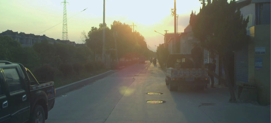
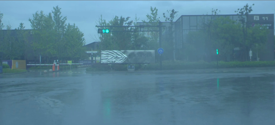
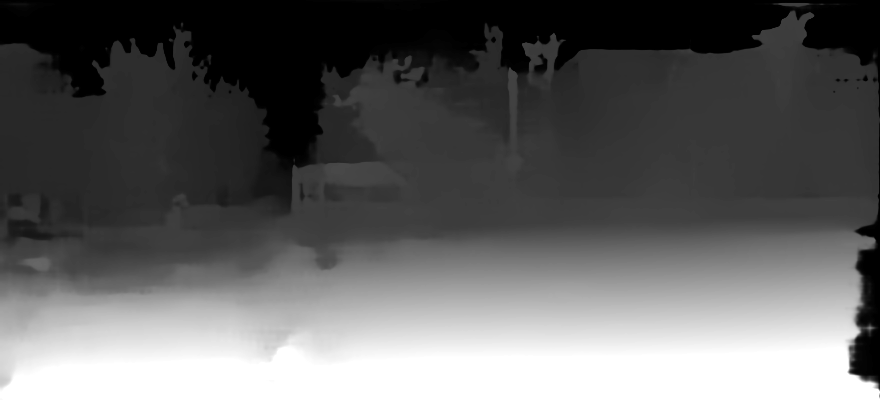
Figure 1: Examples of left images and predicted disparity maps by SEDNet on DrivingStereo [36]. The first example is taken around sunset with over-exposure. The second example is taken on a rainy day with under-exposure. In both challenge cases, SEDNet predicts accurate disparity.

In this paper, we present an implementation of this concept via a deep network that jointly estimates disparity and its uncertainty from a pair of rectified images. We named the network SEDNet, for Stereo Error Distribution Network. SEDNet includes a novel, lightweight uncertainty estimation subnetwork that predicts the aleatoric uncertainty of stereo matching, and a new loss to match the distribution of uncertainties with that of disparity errors. To generate the inputs to this new loss, we approximate the distributions from the samples of disparity errors and uncertainty values in a differentiable way via a soft-histogramming technique.

We present extensive experimental validation of SEDNet’s performance in disparity estimation and uncertainty prediction on large datasets with ground truth. SEDNet is superior to baselines with similar, even identical, architecture, but without the proposed loss function. Our main contributions are:

• a novel uncertainty estimation subnetwork that extracts information from the intermediate multi-resolution disparity maps generated by the disparity subnetwork,

• a differentiable soft-histogramming technique used to approximate the distributions of disparity errors and estimated uncertainties,

• a loss based on KL divergence applied on histograms obtained with the above technique.

2 Related Work

We refer readers to recent surveys on deep stereo matching [32] and on confidence estimation [30]. Here we summarize the most relevant publications to our work.

Stereo matching networks operate on a cost volume, which aggregates 2D features at each potential disparity for every pixel, and can be constructed via correlation or concatenation. Correlation-based networks such as DispNetC [25], iResNet [24] and SegStereo [38], generate a single-channel correlation map between features extracted from the two views at each disparity level, favoring computation efficiency at the expense of losing the structural and semantic information in the feature representation. Concatenation-based networks, such as GCNet [16], PSMNet [2] and GANet [39], assemble features from both views at the disparity specified by the corresponding element of the cost volume. This promotes learning of contextual features but requires more parameters and a subsequent aggregation network.

We select GwcNet [11] as the foundation of our network. GwcNet takes a hybrid approach by reducing the dimension of the unary feature channels before concatenation in the cost volume. This is accomplished by a Group Wise Correlation layer, which takes as input $N_{c}$ unary feature channels, divides them into $N_{g}$ groups, computes the correlation between channels in each group at all disparity levels, and uses the resulting correlation scores to form the cost volume. This reduces the size of the cost volume and the computational cost of 3D convolutions by a factor of $N_{c}:N_{g}$, with $N_{g}$ much smaller than $N_{c}$, but still provides rich similarity-measure features to the disparity estimator.

Researchers have also focused on model reliability. In Bayesian Neural Networks (BNNs), different models are sampled from the distribution of weights to estimate the mean and variance of the target distribution in an empirical manner, yielding estimates of uncertainty [27, 7]. Additional empirical strategies such as Bootstrapped Ensembles [23] and Monte Carlo Dropout [8] also sample from the distribution of weights. On the other hand, Graves [10] and Blundell et al. [1] proposed to replace the sampling with variational inference.

Due to the high cost of training BNNs, methods for modeling the uncertainty or confidence in a predictive manner have also attracted interest. We distinguish between confidence and uncertainty: confidence is a binary variable trained with the BCE loss, while uncertainty is a continuous variable trained with L1 or L2 loss. Nix and Weigend [28] introduce NNs with one output for model prediction and one for data noise (aleatoric uncertainty). In addition to aleatoric uncertainty which captures the data noise of the observations, epistemic uncertainty, which accounts for the uncertainty of the model parameters, can also be modeled  [3]. To capture both types, Kendall et al. [14, 15] proposed to combine empirical and predictive methods in a joint framework.

CNNs have been used to estimate confidence in stereo matching. The Confidence CNN (CCNN) [31], Patch Based Confidence Prediction (PBCP) [33], the Early Fusion Network (EFN) and the Late Fusion Network (LFN) [4] and Multi Modal CNN (MMC)[5] only use small patches of the disparity maps. Conversely, the Global Confidence Network (ConfNet) and the Local-Global Confidence Network (LGC) [35] introduce U-Net like architectures and take both the image and disparity map as inputs. As a baseline, we use the Locally Adaptive Fusion Network (LAF) [18] which predicts the confidence map based on tri-modal inputs: the cost and disparity maps and the color image. An extension based on knowledge distillation has also been published [17]. These strategies are effective and cheaper than the empirical ones, since they only require one forward pass.

Only a subset of the confidence estimation literature has focused on joint disparity and confidence estimation. The Reflective Confidence Network (RCN) [34] is the first to combine a disparity and a confidence loss. The Unified Confidence Network (UCN) [19] and the Adversarial Confidence Network (ACN) [20] jointly estimate confidence and disparity from pre-computed cost volumes. UCN is self-supervised, while ACN combines a generative cost aggregation network and a discriminative confidence estimation network in an adversarial manner. Mehltretter [26] presents an approach that predicts both epistemic and aleatoric uncertainty using a Bayesian Neural Network, based on GCNet [16]. KL divergence is used to measure the distance between the approximation of the distribution of network parameters estimated by variational difference and the exact posterior distribution. (It should be noted that we use KL divergence for a completely different purpose on the distribution of disparity errors.)

Relevant research in adjacent areas of computer vision includes the work of Poggi et al. [29] who comprehensively evaluate uncertainty estimation for self-supervised monocular depth estimation. Ilg et al. [13] study empirical ensembles, predictive models and predictive ensembles as uncertainty models for optical flow estimation.

3 Method

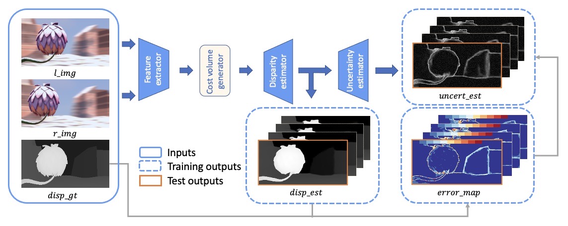
Figure 2: An illustration of SEDNet. The stereo matching subnetwork consists of the feature extractor, cost volume generator and disparity estimator. It takes a rectified pair of images as input and predicts disparity maps at multiple resolutions. The uncertainty estimation subnetwork takes the predicted disparity maps as input and predicts corresponding uncertainty maps. The error maps, between the ground truth and predicted disparity, are used to supervise uncertainty estimation. During training, the network keeps the output at all resolutions, but returns only the highest resolution disparity and uncertainty maps during testing.

The objective of our work is to jointly estimate the disparity and its uncertainty. An important benefit of this joint formulation is that the multi-task network learns to predict more accurate disparities than the standalone disparity estimator when the uncertainty subnetwork is added. Given a stereo image pair $\mathbf{X}=\{\mathbf{x}_{l},\mathbf{x}_{r}\}$, with image dimensions $H\times W$, and the corresponding ground truth disparity $\mathbf{d}$, the prediction ${\hat{\mathbf{d}}}$ of a stereo-matching network ${f_{\theta}}$ can be represented as $\hat{\mathbf{d}}=f_{\theta}(\mathbf{x}_{l},\mathbf{x}_{r})$. For each pixel $i$, the error $\epsilon^{(i)}$ of the prediction is calculated using the L1 loss.

Kendall and Gal [14] use the negative log-likelihood of the prediction model as the loss function to be minimized in pixel-wise tasks. We take the formulation a step further by requiring that the network generate a distribution of uncertainties that matches the distribution of errors. To this end, we propose to minimize the divergence $\mathcal{D}$ between the distributions of predicted uncertainty and actual disparity error.

In the following subsections, we present aleatoric uncertainty estimation (Section 3.1), the proposed KL divergence loss (Section 3.2), our network architecture (Section 3.3), and the combined loss function (Section 3.4).

3.1 Aleatoric Uncertainty Estimation

In order to predict uncertainty and reduce the impact of noise, Kendall and Gal [14] minimize the pixel-wise negative log-likelihood of the prediction model, assuming that it follows a Gaussian distribution. The subsequent work of Ilg et al. [13] shows that the predicted distribution can be modeled as either Laplacian or Gaussian depending on whether the L1 or L2 loss is used for disparity estimation. Since we use the former, we can write the prediction model as:

$$p(\mathbf{d}|f_{\theta}(\mathbf{X}))=\mathcal{L}aplace(f_{\theta}(\mathbf{X}),\sigma)$$ (1)

where the mean is given by the model output and $\sigma$ is the observation noise scalar.

To model aleatoric uncertainty, Kendall and Gal [14] introduce pixel-specific noise parameters $\sigma^{(i)}$. We follow the approach of Ilg et al. [13], who do the same for a Laplacian model, and obtain the following pixel-wise loss function:

$$\mathcal{L}_{log}=\frac{1}{n}\sum^{n}_{i=1}\frac{|\hat{\mathbf{d}}^{(i)}-\mathbf{d}^{(i)}|}{\exp(\mathbf{s}^{(i)})}+\frac{1}{n}\sum^{n}_{i=1}\mathbf{s}^{(i)}$$ (2)

where $\hat{\mathbf{d}}^{(i)}$ and $\mathbf{d}^{(i)}$ are the predicted and ground truth disparity for pixel $i$, $\mathbf{s}^{(i)}$ is the log of the observation noise scalar $\mathbf{\sigma}^{(i)}$, and $n$ is equal to the total number of the pixels. Equation (2) may be viewed as a robust loss function where the residual loss for a pixel is attenuated by its uncertainty, while the second term acts as a regularizer. We follow the authors’ suggestion and train the network to predict the log of the observation noise scalar, $s$, for numerical stability.

3.2 Matching the Distribution of Errors

Training a model using Eq. (2) as the loss improves disparity estimation accuracy and favors uncertainty estimates correlated with the errors. Ideally, we would like each uncertainty estimate to be a precise predictor of the corresponding disparity error. Since this is infeasible, we would like the distribution of uncertainties to match the distribution of errors.

The Kullback-Leibler (KL) divergence [22] is a natural choice for measuring the dissimilarity between the distribution of $\epsilon$ and that of $\sigma$. Since the KL divergence is asymmetric, we choose the distribution of $\epsilon$ as the reference. Therefore, our network should also minimize the following objective function:

$$\mathcal{L}_{div}=\mathcal{D}(P_{\sigma}(d))\|Q_{\epsilon}(d))=\int_{0}^{d_{max}}P_{\sigma}(d)\log\frac{P_{\sigma}(d)}{Q_{\epsilon}(d)}\,dd$$ (3)

where $d$ spans the disparity range. Since the network regresses disparity, the continuous formulation of KL divergence is appropriate.

Minimizing Eq. (3) directly requires closed form expressions for the two distributions, which are not available to us. They could be modeled as Laplace distributions, but the maximum likelihood estimator is not differentiable. Moreover, fitting models to the data may be imprecise at the tails of the distributions. Therefore we choose non-parametric representations in the form of histograms.

Histogramming is also not a differentiable operation, leading us to soft-histogramming as a differentiable alternative. We specify a set of bins for the histograms based on the statistics of the errors $\epsilon$, since their distribution is the one that should be matched by the distribution of uncertainty estimates $\sigma$. Since the L1 loss, and our network in general, does not discriminate between positive and negative errors, we work with absolute values of $\epsilon$ and $\sigma$.

For each batch during training, we compute the mean and standard deviation of the error, $\mu_{\epsilon}$ and $b_{\epsilon}$, set $C_{0}=\mu_{\epsilon}$ as the center of the first bin, and $C_{m}=\mu_{\epsilon}+\alpha_{m}b_{\epsilon}$ as the center of the last bin. (We use $b_{\epsilon}$ for the standard deviation to avoid overloading $\sigma$ or $s$. Also note that the last bin extends to the disparity range, which is also the maximum possible error.) We then define $m-1$ centers evenly spaced in a linear or logarithmic scale between the first and last center.

Given the bin centers, we compute a soft-histogram for the errors and one for the uncertainties as follows, considering all pixels with ground truth disparity, and error values. We present the steps for $\epsilon$ here. For each error $\epsilon^{(i)}$, we compute weights for every bin center which are inversely proportional to the distance.

$$w_{j}(\epsilon^{(i)})=\lambda_{1}\cdot\exp(-\frac{(\mu_{\epsilon}+\alpha_{j}b_{\epsilon}-\epsilon^{(i)})^{2}}{\lambda_{2}})$$ (4)

where $\lambda_{1}$ and $\lambda_{2}$ are hyper-parameters. Softmax is then applied to favor the nearest bins and the contributions of $n$ pixels are accumulated in the bins of the histogram $H_{\epsilon}$.

$$H_{\epsilon}(j) =\frac{1}{n}\sum^{n}_{i=1}\frac{\exp(w_{j}(\epsilon^{(i)}))}{\sum^{m}_{j=0}\exp(w_{j}(\epsilon^{(i)}))},\,\,j\in[0,m]$$ (5)

The histogram for $\sigma$, $H_{\sigma}$, is obtained similarly. (Note that the bins of both histograms are defined in terms of $b_{\epsilon}$.)

The loss representing the discrete form of the KL divergence between the two histograms is given by:

$$\mathcal{L}_{div}=\sum_{j=0}^{m}H_{\epsilon}(j)\log\frac{H_{\epsilon}(j)}{H_{\sigma}(j)}$$ (6)

3.3 SEDNet

Our network architecture, named SEDNet, includes a disparity estimation subnetwork, an uncertainty estimation subnetwork, and is shown in Figure 2. In all experiments, we have adopted GwcNet [11] as the disparity estimation subnetwork, among other options, and we have designed a novel uncertainty estimation subnetwork that interfaces with GwcNet. It is worth noting that the uncertainty subnetwork is extremely small.

The GwcNet subnetwork extracts features from the images using a ResNet-like feature extractor, generates the cost volume, and assigns disparities to pixels using the soft-argmax operator [16]. The output module of the disparity predictor generates $K$ disparity maps at different resolutions.

We propose a new uncertainty estimator integrated with the stereo matching network. The uncertainty estimation subnetwork learns to predict the log of the observation noise scalar, the error, at each pixel. The proposed subnetwork takes the multi-resolution disparity predictions as input, computes the pairwise differences vector (PDV) and passes it to a pixel-wise MLP to regress the uncertainty maps. Specifically, the disparity estimator outputs $K$ disparity maps at different resolutions $\hat{\mathbf{d}}=\{\hat{\mathbf{d}}_{1},...,\hat{\mathbf{d}}_{K}\}$, which are first upsampled to full-resolution and then undergo pairwise differencing to form the PVD, which consists of $K\choose 2$ elements. The output set of uncertainty maps $\mathbf{S}$ also contains $K$ resolutions to match the disparity maps. We use $K=4$ in all experiments.

3.4 Loss Function

Our loss function combines two parts: (1) the log-likelihood loss to optimize the error and uncertainty, (2) the KL divergence loss to match the distribution of uncertainty with the error. The total loss considers all disparity and uncertainty maps upsampled to the highest resolution:

$$\mathcal{L}=\sum^{K}_{k=1}c_{k}\cdot(\mathcal{L}_{log,k}+\mathcal{L}_{div,k})$$ (7)

where $c_{k}$ denotes the coefficients for the $k^{th}$ resolution level, $\mathcal{L}_{log,k}$ and $\mathcal{L}_{div,k}$ are computed by Eq. (2) and Eq. (6) on the prediction of the corresponding resolution level.

4 Experiment Results

Dataset Method Loss Inliers Disparity$\downarrow$ APE$\downarrow$ AUC$\downarrow$ BCE L1 Log KL Bins Scale Def. Pct(%) EPE D1(%) Avg. Median Opt. Est. Scene Flow GwcNet - $\surd$ - - - - - - 0.7758 4.127 - - 10.9291 - +LAF $\surd$ - - - - - - - 0.7758 4.127 - - 10.9291 20.0813 +$\mathcal{L}_{log}$ - $\surd$ $\surd$ - - - EPE<5 96.96 0.7611 4.131 0.6999 0.0728 5.7449 12.1121 +SEDNet - $\surd$ $\surd$ $\surd$ 11 log EPE<$\mu_{\epsilon}$+3$b_{\epsilon}$ 98.42 0.6754 3.963 0.5797 0.0432 4.9134 8.7195 VK2-S6 GwcNet - $\surd$ - - - - - - 0.4125 1.763 - - 6.0962 - +$\mathcal{L}_{log}$ - $\surd$ $\surd$ - - - EPE<5 98.86 0.3899 1.584 0.4136 0.1753 4.6872 12.5320 +SEDNet - $\surd$ $\surd$ $\surd$ 11 log EPE<$\mu_{\epsilon}$+3$b_{\epsilon}$ 99.24 0.3109 1.392 0.5234 0.1454 4.1726 9.7637 +SEDNet - $\surd$ $\surd$ $\surd$ 11 log EPE<$\mu_{\epsilon}$+5$b_{\epsilon}$ 99.68 0.3236 1.427 0.3561 0.1096 4.2767 9.9843 VK2-S6-Moving GwcNet - $\surd$ - - - - - - 0.4253 1.689 - - 5.9184 - +$\mathcal{L}_{log}$ - $\surd$ $\surd$ - - - EPE<5 98.91 0.4231 1.537 0.4575 0.1890 4.3663 11.3532 +SEDNet - $\surd$ $\surd$ $\surd$ 11 log EPE<$\mu_{\epsilon}$+3$b_{\epsilon}$ 99.62 0.3577 1.389 0.5958 0.1573 3.9012 8.8339 +SEDNet - $\surd$ $\surd$ $\surd$ 11 log EPE<$\mu_{\epsilon}$+5$b_{\epsilon}$ 99.76 0.3862 1.420 0.4002 0.1164 4.0423 9.0631 DrivingStereo +$\mathcal{L}_{log}$(FT) - $\surd$ $\surd$ - - - - - 0.5332 0.2641 0.3449 0.2297 21.7002 45.7096 +SEDNet(FT) - $\surd$ $\surd$ $\surd$ 11 log EPE<$\mu_{\epsilon}$+5$b_{\epsilon}$ 99.86 0.5264 0.2439 0.3324 0.2267 21.2856 44.3297 DS-Weather GwcNet - $\surd$ - - - - - - 1.6962 8.313 - - 44.4896 - +$\mathcal{L}_{log}$ - $\surd$ $\surd$ - - - EPE<5 95.78 2.3944 6.666 2.1443 0.4383 41.1909 95.4264 +SEDNet - $\surd$ $\surd$ $\surd$ 11 log EPE<$\mu_{\epsilon}$+3$b_{\epsilon}$ 98.95 1.5637 6.508 2.3406 0.5309 38.4871 86.1118 +SEDNet - $\surd$ $\surd$ $\surd$ 11 log EPE<$\mu_{\epsilon}$+5$b_{\epsilon}$ 99.41 1.7051 6.057 1.5842 0.6104 39.8057 87.1882

Table 1: Quantitative results: (1) within-domain on SceneFlow, VK2-S6 and VK2-S6-Moving; (2) after finetuning (FT) on DrivingStereo; (3) cross-domain on DS-Weather. The best results in each category in each experiment are in bold typeface. SEDNet outperforms the baselines with respect to disparity and uncertainty metrics in the majority of experiments.

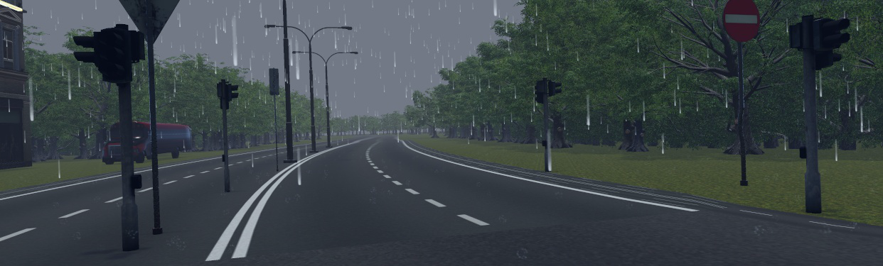
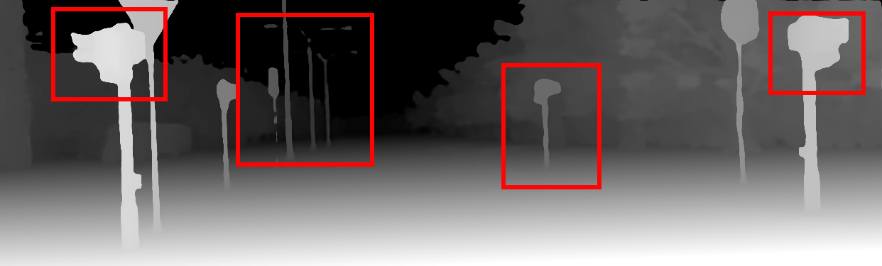
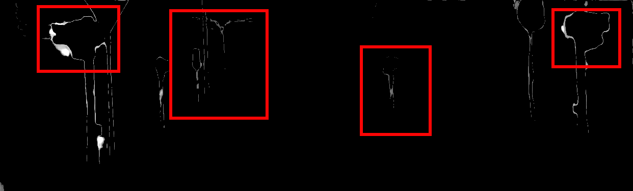
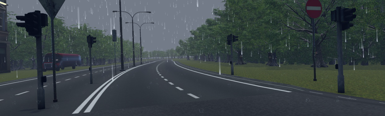
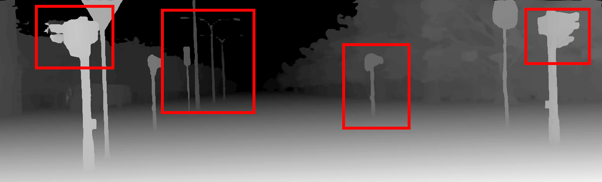
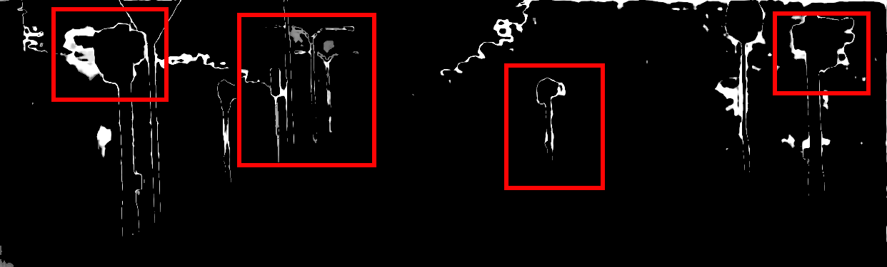
Left Image $\mathcal{L}_{log}$ Disparity $\mathcal{L}_{log}$ Uncertainty Right Image SEDNet Disparity SEDNet Uncertainty

Figure 3: Example from VK2-S6. In a rainy scene with poor illumination, recognizing objects far away from the camera is even difficult for human observers. $\mathcal{L}_{log}$ fails to predict the disparity of objects, such as the traffic sign near the left street light. On the other hand, SEDNet accurately predicts the disparity of these challenging objects, while its uncertainty map also captures more information, such as the trees in the background, the traffic light near the trees and the street lights.

In this section, we present our experimental setup and results on within-domain and cross-domain experiments. Datasets, evaluation metrics and baselines are described in Section 4.1, implementation details in Section 4.2, and experimental results in Sections 4.3 and 4.4. Additionally, a synthetic-to-real transfer evaluation is presented in Section 4.5. We provide more quantitative and qualitative results, extending Section 4, in the Supplement, which also includes ablation studies on several aspects of SEDNet and the baselines, as well as disparity, error, and uncertainty maps of difficult examples.

4.1 Datasets and evaluation metrics

SceneFlow [25] is a collection of three synthetic stereo datasets: FlyingThings3D, Driving, Monkaa. The datasets provide $35,454$ training and $4,370$ test stereo pairs in $960\times 540$ pixel resolution with dense ground-truth disparity maps. We use the finalpass versions of the rendered images which are more realistic because of the motion blur and depth of field effect.

Virtual KITTI 2 (VK2) [6] is a synthetic clone of KITTI [9]. It consists of $21,260$ synthetic $1,242\times 375$ stereo pairs from 6 driving scenes with 10 different imaging and weather conditions. Scene 006 (VK2-S6) is specified as the test set by the authors of the dataset. Since the car with the cameras is stopped for a long part of Scene 006 and only other cars move in the images, we split the last part of the scene where the car moves and denote it as VK2-S6-Moving. We report results separately on this subset. Since results on VK2-S6-Moving do not suffer from bias due to the almost constant background of the first part of the scene, evaluation on VK2-S6-Moving is more informative and fair.

DrivingStereo [37] is a large real-world autonomous driving dataset. It contains $174,437$ training and $7,751$ test stereo pairs at $881\times 400$ pixel resolution. The dataset provides sparse ground truth disparity as well as a challenging subset (DS-Weather) of $2,000$ stereo pairs in 4 different weather conditions.

For all datasets above, we exclude pixels with disparities $d>192$ in training.

Metrics. To evaluate disparity estimation, we compute the endpoint error (EPE) and the percentage of outliers (D1) (i.e., the percentage of pixels with EPE $>3$px or $\geq 5\%$ of the true depth).

To evaluate uncertainty estimation, we use density-EPE ROC curves and the area under the curve (AUC) [30, 12, 18]. The ROC curves in our case measure EPE (not binary correctness) at increasing disparity map density by successively adding pixels in increasing order of uncertainty. The optimal AUC is obtained by adding pixels in order of increasing EPE and is therefore the lowest value any algorithm could achieve given the set of EPE values, while the estimated AUC is sorted by predicted uncertainty. To evaluate the precision of uncertainty estimation, we also introduce the absolute prediction error (APE), which is the average L1 distance between the error and the observation noise scalar, $\sigma$. We report the average and median APE over all pixels.

Baselines. Since we use GwcNet [11] as the disparity estimation subnetwork of SEDNet, we compare SEDNet with three baselines: (1) the original GwcNet trained with smooth L1 loss. (2) LAF-Net [18] trained under the BCE loss on the left RGB images, the cost volumes and predicted disparity maps of GwcNet at the highest resolution. (3) SEDNet but only trained with the log-likelihood loss, therefore similar to Kendall and Gal’s model [14]. We use $\mathcal{L}_{log}$ in tables and figures for this baseline. We selected GwcNet because it is the backbone of SEDNet, and LAF-Net as the confidence estimation baseline due to its strong performance within the training domain according to [30].

4.2 Implementation Details

We implemented all networks in PyTorch and used the Adam optimizer [21] with $\beta_{1}=0.9$ and $\beta_{2}=0.999$ for all experiments. Training of all models was stopped before overfitting occurred.

Experiments on the VK2 dataset were performed on two NVIDIA RTX A6000 GPUs, each with 48 GB of RAM. For this dataset, we trained all models from scratch with an initial learning rate of 0.0001, down-scaled by 5 every 10 epochs. During training, we randomly cropped $512\times 256$ patches from the images. During testing, we evaluated at the full resolution of VK2.

Experiments on the DrivingStereo dataset (DS) were also performed on two NVIDIA RTX A6000 GPUs. For this dataset, we did two experiments using the models pre-trained on VK2: (1) we finetuned on the DS training set with a learning rate starting from 0.0001, down-scaled by 2 every 3 epochs after epoch 10, then performed in-domain evaluation on the DS test set; (2) we skipped the finetuning step and performed cross-domain evaluation on DS-Weather subset. During training, we randomly cropped the inputs to be the same size as in the VK2 experiments. During testing, we padded the test samples to be the same resolution as VK2.

Architecture	Params	MACs(G)
GwcNet	6,909,728	1075.82
SEDNet	6,909,918	1075.91

Table 2: Comparison on number of parameters and computational complexity. MAC stands for multiply–accumulate operations. SEDNet only adds a 3-layer MLP, with 190 parameters, as an uncertainty decoder to GwcNet.

Experiments on the SceneFlow dataset were performed on an Nvidia TITAN RTX GPU with 24 GB memory. We trained all models from scratch on $256\times 128$ patches cropped from half-resolution images to limit memory consumption. We set the initial learning rate to 0.001 and down-scaled it by 2 every 2 epochs after epoch 10.

For all the experiments above, we applied an inlier filtering strategy during training, which only back-propagates from the inliers. See the last paragraph of Section 4.3 for details. Table 2 shows the number of parameters and computational complexity of GwcNet and SEDNet.

4.3 Qualitative and Quantitative Results

In Table 1, we present results: (1) within-domain on SceneFlow and VK2; (2) on the DrivingStereo test set after finetuning the VK2 models on the DrivingStereo training set; (3) cross-domain on the DS-Weather challenge test set by directly applying the model trained on VK2 without finetuning. An extended version of this table can be found in Table S.1 in the Supplement.

Disparity Estimation. In all experiments, SEDNet achieves lower errors than all the baselines. See the EPE and D1 columns in Table 1. Even in extreme weather like fog and rain, SEDNet predicts good disparity unaffected by poor illumination and blur. See Figure 3.

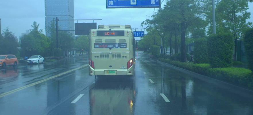
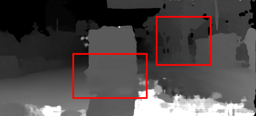
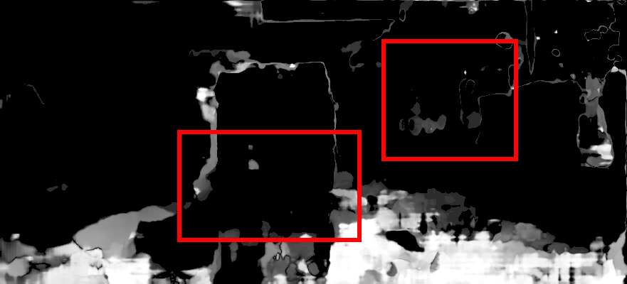
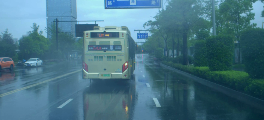
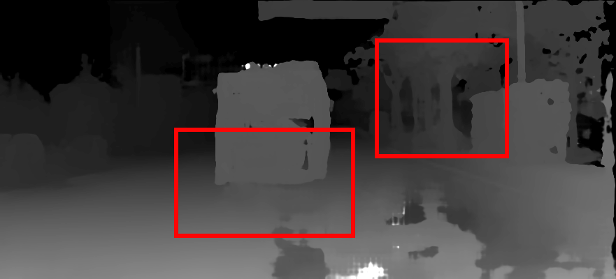
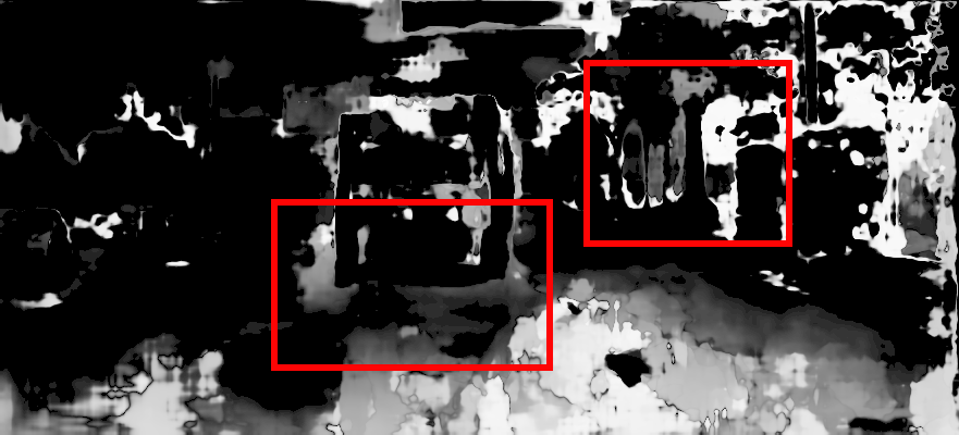
Left Image $\mathcal{L}_{log}$ Disparity $\mathcal{L}_{log}$ Uncertainty Right Image SEDNet Disparity SEDNet Uncertainty

Figure 4: Example from DS-Weather. Unlike the synthetic data, the rainy-day real images do not only suffer from poor illumination, but also pose challenges due to reflections in the water. In this example, the road is like a mirror, misleading the $\mathcal{L}_{log}$ model. Recall that the LIDAR ground truth disparity is very sparse, and is even sparser in reflective regions. The disparity map of $\mathcal{L}_{log}$ fails to distinguish the car and the reflection, but SEDNet is able to estimate the correct disparity and the uncertainty of the car.

Uncertainty Estimation. Our method outperforms the baselines in all experiments according to the AUC metric, as shown in the last two columns in Table 1. Compared to $\mathcal{L}_{log}$, SEDNet decreases the estimated AUC by $20\%$ – $30\%$ in the in-domain experiments, with a $10\%$ decrease in optimal AUC, which depends on EPE. In the cross-domain evaluation, the advantage of SEDNet is even more evident. Figure 4 shows uncertainty maps for real data, on which our method captures details more faithfully. The ROC curves of the best $\mathcal{L}_{log}$ and SEDNet models based on EPE on VK2-S6-Moving are presented in Figure 5.

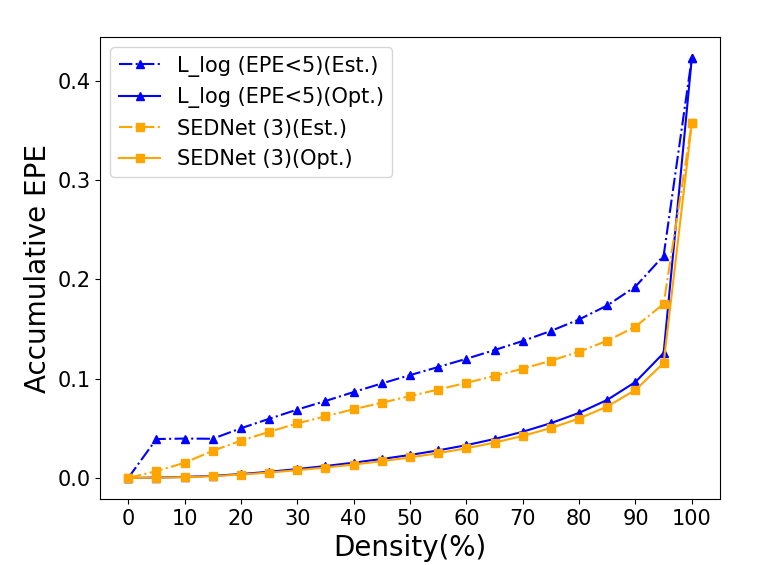
Figure 5: Comparison of density-EPE curves on VK2-S6-Moving. ”L_log (EPE<5)” and ”SEDNet (3)” represent the $\mathcal{L}_{log}$ (with fixed inliers) and the SEDNet (with adaptive inliers of EPE<$\mu_{\epsilon}$+3$b_{\epsilon}$) of the VK2-S6-Moving experiment in Table 1. While their corresponding optimal AUCs are almost equal, the advantage of SEDNet in estimated AUC is significant.

Effects of Back-propagation from Inliers. We apply two kinds of inlier filters: one with a fixed threshold that excludes all pixels that have an EPE larger than 5 from back-propagation; and one with adaptive threshold which excludes pixels that have EPE greater than a specified number of $b_{\epsilon}$ from the mean error. Back-propagation from the inliers only helps the network improve its performance on both disparity and uncertainty estimation. We attribute this to the suppression of harmful outliers that give rise to large gradients. Quantitative results for the baselines and the proposed method with different inlier settings are reported in the Supplement. The results show that using adaptive thresholds is better than fixed thresholds. Fixed thresholds exclude more pixels, especially at lower resolutions and in the early stages of training, preventing the network from learning how to correct them.

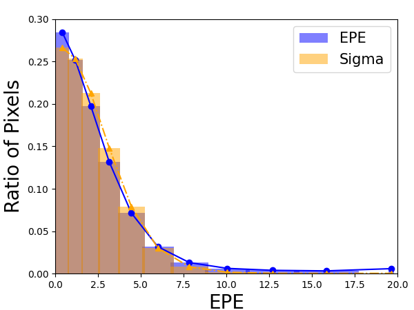
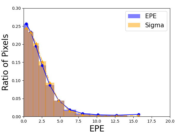
$\mathcal{L}_{log}$ SEDNet

Figure 6: Distribution of error and predicted uncertainty. We pick the best model of $\mathcal{L}_{log}$ and SEDNet in VK2-S6-Moving, then randomly sample $5,000,000$ points from the outputs of the two models. The distributions of error and $\sigma$ of SEDNet are much closer than those of the $\mathcal{L}_{log}$ model, especially in the first 5 bins that contain more than 95% of the samples. The shorter tail of SEDNet also indicates fewer gross errors.

Dataset Method Loss Inliers Disparity$\downarrow$ APE$\downarrow$ AUC$\downarrow$ BCE L1 Log KL Bins Scale Def. Pct(%) EPE D1(%) Avg. Median Opt. Est. VK2-S6-Morning GwcNet - $\surd$ - - - - - - 0.4642 1.740 - - 6.1845 - +$\mathcal{L}_{log}$ - $\surd$ $\surd$ - - - EPE<5 98.82 0.4774 1.624 0.5067 0.1872 4.6698 12.5192 +SEDNet - $\surd$ $\surd$ $\surd$ 11 log EPE<$\mu_{\epsilon}$+3$b_{\epsilon}$ 99.62 0.4003 1.442 0.6183 0.1553 4.1847 9.4063 VK2-S6-Sunset GwcNet - $\surd$ - - - - - - 0.4810 1.825 - - 6.6907 +$\mathcal{L}_{log}$ - $\surd$ $\surd$ - - - EPE<5 98.84 0.4863 1.627 0.5060 0.1827 5.0075 13.7848 +SEDNet - $\surd$ $\surd$ $\surd$ 11 log EPE<$\mu_{\epsilon}$+3$b_{\epsilon}$ 99.61 0.4108 1.475 0.6189 0.1509 4.5840 10.7946 VK2-S6-Fog GwcNet - $\surd$ - - - - - - 0.4660 1.812 - - 6.8355 - +$\mathcal{L}_{log}$ - $\surd$ $\surd$ - - - EPE<5 98.98 0.4425 1.448 0.4609 0.1865 4.8983 12.1305 +SEDNet - $\surd$ $\surd$ $\surd$ 11 log EPE<$\mu_{\epsilon}$+3$b_{\epsilon}$ 99.71 0.3731 1.288 0.5517 0.1547 4.4200 9.9380 VK2-S6-Rain GwcNet - $\surd$ - - - - - - 0.4618 1.700 - - 6.6774 - +$\mathcal{L}_{log}$ - $\surd$ $\surd$ - - - EPE<5 98.88 0.4707 1.571 0.4899 0.1861 4.9351 13.3214 +SEDNet - $\surd$ $\surd$ $\surd$ 11 log EPE<$\mu_{\epsilon}$+3$b_{\epsilon}$ 99.69 0.3873 1.356 0.6685 0.1537 4.4013 10.3362 DS-Cloudy GwcNet - $\surd$ - - - - - - 1.3413 5.229 - - 37.4263 - +$\mathcal{L}_{log}$ - $\surd$ $\surd$ - - - EPE<5 97.48 1.4780 3.948 1.2617 0.3513 34.4488 82.5380 +SEDNet - $\surd$ $\surd$ $\surd$ 11 log EPE<$\mu_{\epsilon}$+3$b_{\epsilon}$ 98.83 1.3183 4.414 1.5260 0.4021 33.9037 73.6330 DS-Sunny GwcNet - $\surd$ - - - - - - 1.5448 6.991 - - 38.7386 - +$\mathcal{L}_{log}$ - $\surd$ $\surd$ - - - EPE<5 97.08 1.4837 4.631 1.2806 0.3835 35.5226 85.8715 +SEDNet - $\surd$ $\surd$ $\surd$ 11 log EPE<$\mu_{\epsilon}$+3$b_{\epsilon}$ 98.64 1.5548 5.878 3.0025 0.4808 35.6523 83.2573 DS-Foggy GwcNet - $\surd$ - - - - - - 1.5476 8.859 - - 51.4640 - +$\mathcal{L}_{log}$ - $\surd$ $\surd$ - - - EPE<5 94.89 2.9553 9.015 2.6923 0.5556 48.7136 101.7025 +SEDNet - $\surd$ $\surd$ $\surd$ 11 log EPE<$\mu_{\epsilon}$+3$b_{\epsilon}$ 99.27 1.5398 7.357 2.4109 0.7023 47.7932 97.8627 DS-Rainy GwcNet - $\surd$ - - - - - - 3.1918 17.356 - - 68.0346 - +$\mathcal{L}_{log}$ - $\surd$ $\surd$ - - - EPE<5 98.79 5.3539 12.501 4.9480 0.5759 59.3952 146.8906 +SEDNet - $\surd$ $\surd$ $\surd$ 11 log EPE<$\mu_{\epsilon}$+3$b_{\epsilon}$ 99.10 2.2165 11.020 2.6599 0.6722 50.8103 110.8360

Table 3: Quantitative results of synthetic to real evaluation. The top 4 subsets from VK2-S6-Moving are synthetic datasets, while the rest 4 subsets from DS-Weather are the real dataset. The best results in each category in each experiment are in bold typeface. SEDNet outperforms the baselines especially on the uncertainty estimation of the real data and under terrible weather (i.e., foggy and rainy).

4.4 Matching the Error Distribution.

Comparing the results of APE in all experiments in Table 1 and Figure 6, the difference between the errors and the predicted uncertainty is always close to the EPE, as expected. SEDNet, however, achieves lower APE, showing that it matches the true distribution better.

4.5 Generalization from Synthetic to Real Data

Stereo-matching networks are typically trained on synthetic data and fine-tuned on small amounts of data from the target domain due to the cost and difficulty of acquiring real data with ground truth depth. In this section, we extend the experiments of VK2-S6 and DS-Weather in Table 1 to compare the generalization performance on unseen real domains of all methods trained only on synthetic data. We picked four synthetic subsets from VK2-S6, specifically Morning, Sunset, Fog and Rain, that have similar illumination conditions, visibility level and weather with the four real subsets of DS-Weather [37], i.e., Cloudy, Sunny, Foggy and Rainy. VK2-S6-Morning and VK2-S6-Sunset have similar illumination to DS-Cloudy and DS-Sunny, but the latter two are more challenging due to camera underexposure and overexposure. Even though they are acquired under the same weather, DS-Foggy and DS-Rainy are more difficult than VK2-S6-Fog and VK2-S6-Rain. This can be seen by comparing Figures 3 and 4. The synthetic examples only mimic the poor lighting conditions and challenges caused by the fog and rain, but ignore the Tyndall effect and reflections caused by the fog and stagnant water.

As mentioned above, all models are trained only on Scenes 001, 002, 018 and 020 of VK2. Quantitative results on synthetic to real transfer are reported in Table 3, where we only report the best model of each method. The top-performing variant of SEDNet outperforms the baselines in the majority of experiments. An extended version of this table can be found in Table S.2 in the Supplement.

5 Conclusion

We have presented a novel approach for joint disparity and uncertainty estimation from stereo image pairs. The key idea is a unique loss function based on the KL divergence between the distributions of disparity errors and uncertainty estimates. This is made possible by a differentiable histogramming scheme that we also introduce here. To implement our approach, we extended the GwcNet architecture to include an uncertainty estimation subnetwork with only 190 parameters. Our experiments on multiple large datasets have demonstrated that our approach, named SEDNet, is effective in both disparity and uncertainty prediction. The success of our method is attributed to the novel loss function. SEDNet easily surpasses GwcNet in disparity estimation even though they have essentially the same capacity and almost identical architecture, up to the tiny uncertainty estimation subnetwork. We are optimistic that our approach will be similarly successful in other pixel-wise regression tasks, which we plan to address in future research.

Acknowledgment. This research has been supported in part by the National Science Foundation under award 2024653.

Supplement

In this document, we present more quantitative and qualitative results extending Section 4 of the main paper. Ablation studies on the configuration of the histograms and on different settings of inlier filters are provided in Section S.1. A detailed version of the synthetic-to-real transfer from Virtual KITTI 2 (VK2) to the DrivingStereo weather subsets (DS-Weather) is presented in Section S.2. Section S.3 includes additional qualitative results, such as disparity, error and uncertainty maps.

Appendix S.1 Ablation Studies

Dataset Method Loss Inliers Disparity$\downarrow$ APE$\downarrow$ AUC$\downarrow$ BCE L1 Log KL Bins Scale Def. Pct(%) EPE D1(%) Avg. Median Opt. Est. Scene Flow GwcNet - $\surd$ - - - - - - 0.7758 4.127 - - 10.9291 - GwcNet - $\surd$ - - - - EPE<5 97.09 0.7799 3.940 - - 8.3413 - GwcNet - $\surd$ - - - log EPE<$\mu_{\epsilon}$+3$b_{\epsilon}$ 98.41 0.7981 4.072 - - 9.6451 - +LAF $\surd$ - - - - - - - 0.7758 4.127 - - 10.9291 20.0813 +$\mathcal{L}_{log}$ - $\surd$ $\surd$ - - - - - 0.7445 4.522 0.7133 0.0795 6.2567 10.9635 +$\mathcal{L}_{log}$ - $\surd$ $\surd$ - - - EPE<5 96.96 0.7611 4.131 0.6999 0.0728 5.7449 12.1121 +$\mathcal{L}_{log}$ - $\surd$ $\surd$ - - log EPE<$\mu_{\epsilon}$+3$b_{\epsilon}$ 98.33 0.7890 4.428 0.7047 0.0869 6.6069 12.4265 +SEDNet - $\surd$ $\surd$ $\surd$ - - EPE<5 96.57 1.0046 4.455 0.9092 0.1327 7.1444 16.0036 +SEDNet - $\surd$ $\surd$ $\surd$ 11 lin EPE<$\mu_{\epsilon}$+3$b_{\epsilon}$ 98.42 0.6827 4.022 0.5877 0.0450 5.1258 9.0113 +SEDNet - $\surd$ $\surd$ $\surd$ 11 log EPE<$\mu_{\epsilon}$+3$b_{\epsilon}$ 98.42 0.6754 3.963 0.5797 0.0432 4.9134 8.7195 +SEDNet - $\surd$ $\surd$ $\surd$ 20 log EPE<$\mu_{\epsilon}$+3$b_{\epsilon}$ 98.42 0.6762 3.966 0.5821 0.0433 4.9845 8.8103 +SEDNet - $\surd$ $\surd$ $\surd$ 50 log EPE<$\mu_{\epsilon}$+3$b_{\epsilon}$ 98.42 0.6894 4.016 0.5931 0.0426 5.0216 8.9412 VK2-S6 GwcNet - $\surd$ - - - - - - 0.4125 1.763 - - 6.0962 - GwcNet - $\surd$ - - - - EPE<5 98.82 0.4339 1.634 - - 6.0598 - GwcNet - $\surd$ - - - log EPE<$\mu_{\epsilon}$+3$b_{\epsilon}$ 99.50 0.4597 1.847 - - 6.5506 - +$\mathcal{L}_{log}$ - $\surd$ $\surd$ - - - - - 0.4360 1.957 0.5876 0.1123 4.9389 10.2407 +$\mathcal{L}_{log}$ - $\surd$ $\surd$ - - - EPE<5 98.86 0.3899 1.584 0.4136 0.1753 4.6872 12.5320 +$\mathcal{L}_{log}$ - $\surd$ $\surd$ - - log EPE<$\mu_{\epsilon}$+3$b_{\epsilon}$ 99.52 0.4079 1.673 0.4549 0.2261 5.1675 13.3036 +SEDNet - $\surd$ $\surd$ $\surd$ - - EPE<5 98.59 0.5197 1.905 0.5382 0.1779 5.2803 13.1777 +SEDNet - $\surd$ $\surd$ $\surd$ 11 log EPE<$\mu_{\epsilon}$+1$b_{\epsilon}$ 98.30 0.3896 1.582 0.3876 0.1330 4.4569 11.8449 +SEDNet - $\surd$ $\surd$ $\surd$ 11 log EPE<$\mu_{\epsilon}$+3$b_{\epsilon}$ 99.24 0.3109 1.392 0.5234 0.1454 4.1726 9.7637 +SEDNet - $\surd$ $\surd$ $\surd$ 11 log EPE<$\mu_{\epsilon}$+5$b_{\epsilon}$ 99.68 0.3236 1.427 0.3561 0.1096 4.2767 9.9843 VK2-S6-Moving GwcNet - $\surd$ - - - - - - 0.4253 1.689 - - 5.9184 - GwcNet - $\surd$ - - - - EPE<5 98.85 0.4543 1.593 - - 5.7884 - GwcNet - $\surd$ - - - log EPE<$\mu_{\epsilon}$+3$b_{\epsilon}$ 99.60 0.4708 1.707 - - 6.2409 - +$\mathcal{L}_{log}$ - $\surd$ $\surd$ - - - - - 0.4618 1.930 0.5592 0.1176 4.6928 9.3604 +$\mathcal{L}_{log}$ - $\surd$ $\surd$ - - - EPE<5 98.91 0.4231 1.537 0.4575 0.1890 4.3663 11.3532 +$\mathcal{L}_{log}$ - $\surd$ $\surd$ - - log EPE<$\mu_{\epsilon}$+3$b_{\epsilon}$ 99.63 0.4280 1.632 0.4885 0.2406 4.7709 12.5484 +SEDNet - $\surd$ $\surd$ $\surd$ - - EPE<5 98.67 0.5581 1.823 0.5806 0.1910 4.9404 12.1068 +SEDNet - $\surd$ $\surd$ $\surd$ 11 log EPE<$\mu_{\epsilon}$+1$b_{\epsilon}$ 98.77 0.4220 1.567 0.4277 0.1442 4.1986 10.8037 +SEDNet - $\surd$ $\surd$ $\surd$ 11 log EPE<$\mu_{\epsilon}$+3$b_{\epsilon}$ 99.62 0.3577 1.389 0.5958 0.1573 3.9012 8.8339 +SEDNet - $\surd$ $\surd$ $\surd$ 11 log EPE<$\mu_{\epsilon}$+5$b_{\epsilon}$ 99.76 0.3862 1.420 0.4002 0.1164 4.0423 9.0631 DrivingStereo +$\mathcal{L}_{log}$(FT) - $\surd$ $\surd$ - - - - - 0.5332 0.2641 0.3449 0.2297 21.7002 45.7096 +SEDNet(FT) - $\surd$ $\surd$ $\surd$ 11 log EPE<$\mu_{\epsilon}$+5$b_{\epsilon}$ 99.86 0.5264 0.2439 0.3324 0.2267 21.2856 44.3297 DS-Weather GwcNet - $\surd$ - - - - - - 1.6962 8.313 - - 44.4896 - GwcNet - $\surd$ - - - - EPE<5 73.05 18.2891 30.856 - - 358.1623 - GwcNet - $\surd$ - - - log EPE<$\mu_{\epsilon}$+3$b_{\epsilon}$ 97.87 14.3547 31.835 - - 315.8265 - +$\mathcal{L}_{log}$ - $\surd$ $\surd$ - - - - - 1.9458 8.700 6.2375 0.8295 43.3146 127.4829 +$\mathcal{L}_{log}$ - $\surd$ $\surd$ - - - EPE<5 95.78 2.3944 6.666 2.1443 0.4383 41.1909 95.4264 +$\mathcal{L}_{log}$ - $\surd$ $\surd$ - - log EPE<$\mu_{\epsilon}$+3$b_{\epsilon}$ 98.32 5.4850 15.136 5.1234 0.7290 90.5541 175.9993 +SEDNet - $\surd$ $\surd$ $\surd$ - - EPE<5 94.33 3.7375 9.297 3.3794 0.5249 49.9049 124.0092 +SEDNet - $\surd$ $\surd$ $\surd$ 11 log EPE<$\mu_{\epsilon}$+1$b_{\epsilon}$ 95.54 6.9335 9.346 6.1682 0.4946 53.5638 99.2891 +SEDNet - $\surd$ $\surd$ $\surd$ 11 log EPE<$\mu_{\epsilon}$+3$b_{\epsilon}$ 98.95 1.5637 6.508 2.3406 0.5309 38.4871 86.1118 +SEDNet - $\surd$ $\surd$ $\surd$ 11 log EPE<$\mu_{\epsilon}$+5$b_{\epsilon}$ 99.41 1.7051 6.057 1.5842 0.6104 39.8057 87.1882

Table S.1: Quantitative results: (1) within-domain on SceneFlow, VK2-S6 and VK2-S6-Moving; (2) after finetuning (FT) on DrivingStereo; (3) cross-domain on DS-Weather. The best results in each category in each experiment are highlighted in dark blue. The top-performing variant of SEDNet, namely SEDNet with EPE<$\mu_{\epsilon}$+3$b_{\epsilon}$, outperforms the baselines with respect to disparity and uncertainty metrics in the majority of experiments.

We conduct ablation studies to explore the impact of the number and spacing between the histogram bins, as well as the inlier threshold. Table S.1 summarizes the quantitative results obtained from different baselines and our proposed method trained on the three datasets. (We selected the best variant of each method and presented a brief version of this table as Table 1 in the main paper.)

The first ablation study is to explore the configuration of the histograms, i.e. the $\alpha$ and $m$ in Section 3.2 in the main paper, with respect to the Bins and Scale under Loss category in all tables. We performed this experiment on the Scene Flow dataset. When training SEDNet, we varied the number of bins and toggled between linear and logarithmic scaling. The results reveal that using bins defined in log space is better than linear space. This is due to the fact that the distributions of errors and uncertainty are approximately Laplace distributions, and as a result, most samples are concentrated around the means. See the two rows corresponding to SEDNet with 11 bins in the Scene Flow section of Table S.1 for a comparison of linearly and logarithmically spaced bins. The distributions corresponding to these two rows are also plotted in Figure S.1. Moreover, we find that increasing the number of bins for soft-histogramming does not increase the accuracy but only the computational cost. See the last four rows in the Scene Flow section in Table S.1 that shows SEDNet results with 11, 20 or 50 bins.

Linear bins

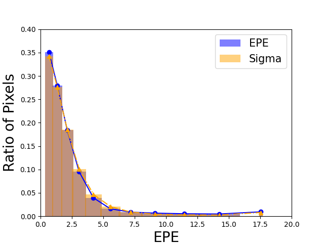
Logarithmic bins

Figure S.1: Distributions of error and predicted uncertainty using different scaling of bins. The distributions correspond to the two rows of SEDNet with 11 bins in the Scene Flow section of Table S.1.

The second ablation study revolves around the selection of the inlier threshold, i.e. the Inliers category in all tables. We first tried GwcNet, $\mathcal{L}_{log}$ and SEDNet with a fixed threshold (EPE<$5$) and then an adaptive threshold (<$\mu_{\epsilon}$+1$b_{\epsilon}$) when training on Scene Flow and VK2. We find that GwcNet and $\mathcal{L}_{log}$ are more compatible with a fixed threshold, while SEDNet works better when using an adaptive threshold. We also changed the threshold of SEDNet to be $\mu_{\epsilon}$+1$b_{\epsilon}$ and $\mu_{\epsilon}$+5$b_{\epsilon}$ when training models on VK2. In most cases, models with the threshold at $3b_{\epsilon}$ are better than others. This does not hold for the evaluation on DS-Weather, where the network lacks knowledge of the unseen domain. Information from the error maps available when the threshold is larger may support a better prediction.

We also computed the precise percentage of the inliers in each experiment, see Pct in Table S.1. The results indicate that the threshold, fixed or adaptive, should not be too restrictive because the network does not improve if back-propagation only occurs on pixels with small errors. At the same time, outliers contaminate the solution and sometimes hinder convergence.

Appendix S.2 Generalization from Synthetic to Real Data

Here, we present more quantitative results on the synthetic to real data experiments supplementing Table 3 in the main paper. Table S.2 presents results from multiple variants of each method, including with and without inlier filtering, and different fixed or adaptive thresholds. The results are consistent with the findings in the ablation studies.

It is worth noting that on DS-Rainy, SEDNet with an inlier threshold of $\mu_{\epsilon}+1b_{\epsilon}$ exhibits very poor performance due to the fact that only 85.82% of the pixels are considered inliers. An overly restrictive inlier threshold, fixed or adaptive, is harmful to the performance of the network, since the back-propagation only occurs on pixels with small errors and the network does not benefit from hard examples.

Dataset Method Loss Inliers Disparity$\downarrow$ APE$\downarrow$ AUC$\downarrow$ BCE L1 Log KL Bins Scale Def. Pct(%) EPE D1(%) Avg. Median Opt. Est. VK2-S6-Morning GwcNet - $\surd$ - - - - - - 0.4642 1.740 - - 6.1845 - GwcNet - $\surd$ - - - - EPE<5 98.79 0.5107 1.649 - - 6.0792 - GwcNet - $\surd$ - - - log EPE<$\mu_{\epsilon}$+3$b_{\epsilon}$ 99.57 0.5065 1.742 - - 6.4706 - +$\mathcal{L}_{log}$ - $\surd$ $\surd$ - - - - - 0.5117 1.998 0.6616 0.1162 5.0563 10.0704 +$\mathcal{L}_{log}$ - $\surd$ $\surd$ - - - EPE<5 98.82 0.4774 1.624 0.5067 0.1872 4.6698 12.5192 +$\mathcal{L}_{log}$ - $\surd$ $\surd$ - 11 log EPE<$\mu_{\epsilon}$+3$b_{\epsilon}$ 99.59 0.4571 1.614 0.5063 0.2231 4.8135 12.2921 +SEDNet - $\surd$ $\surd$ $\surd$ - - EPE<5 98.58 0.6136 1.928 0.6300 0.1897 5.2304 13.1250 +SEDNet - $\surd$ $\surd$ $\surd$ 11 log EPE<$\mu_{\epsilon}$+1$b_{\epsilon}$ 98.83 0.4774 1.626 0.4768 0.1431 4.4936 11.8164 +SEDNet - $\surd$ $\surd$ $\surd$ 11 log EPE<$\mu_{\epsilon}$+3$b_{\epsilon}$ 99.62 0.4003 1.442 0.6183 0.1553 4.1847 9.4063 +SEDNet - $\surd$ $\surd$ $\surd$ 11 log EPE<$\mu_{\epsilon}$+5$b_{\epsilon}$ 99.71 0.4265 1.481 0.4356 0.1150 4.3216 9.6694 VK2-S6-Sunset GwcNet - $\surd$ - - - - - - 0.4810 1.825 - - 6.6907 - GwcNet - $\surd$ - - - - EPE<5 98.76 0.5222 1.701 - - 6.5110 - GwcNet - $\surd$ - - - log EPE<$\mu_{\epsilon}$+3$b_{\epsilon}$ 99.57 0.5345 1.795 - - 6.9508 - +$\mathcal{L}_{log}$ - $\surd$ $\surd$ - - - - - 0.5112 2.040 0.6134 0.1137 5.4426 11.1299 +$\mathcal{L}_{log}$ - $\surd$ $\surd$ - - - EPE<5 98.84 0.4863 1.627 0.5060 0.1827 5.0075 13.7848 +$\mathcal{L}_{log}$ - $\surd$ $\surd$ - 11 log EPE<$\mu_{\epsilon}$+3$b_{\epsilon}$ 99.62 0.4678 1.646 0.5046 0.2151 5.2551 13.8256 +SEDNet - $\surd$ $\surd$ $\surd$ - - EPE<5 98.54 0.6506 1.981 0.6558 0.1827 5.7348 14.6926 +SEDNet - $\surd$ $\surd$ $\surd$ 11 log EPE<$\mu_{\epsilon}$+1$b_{\epsilon}$ 98.81 0.4871 1.664 0.4764 0.1356 4.9970 13.4379 +SEDNet - $\surd$ $\surd$ $\surd$ 11 log EPE<$\mu_{\epsilon}$+3$b_{\epsilon}$ 99.61 0.4108 1.475 0.6189 0.1509 4.5840 10.7946 +SEDNet - $\surd$ $\surd$ $\surd$ 11 log EPE<$\mu_{\epsilon}$+5$b_{\epsilon}$ 99.72 0.4422 1.505 0.4399 0.1103 4.8745 11.0680 VK2-S6-Fog GwcNet - $\surd$ - - - - - - 0.4660 1.812 - - 6.8355 - GwcNet - $\surd$ - - - - EPE<5 98.91 0.4817 1.556 - - 6.4733 - GwcNet - $\surd$ - - - log EPE<$\mu_{\epsilon}$+3$b_{\epsilon}$ 99.66 0.5073 1.810 - - 7.1501 - +$\mathcal{L}_{log}$ - $\surd$ $\surd$ - - - - - 0.4919 1.859 0.5574 0.1174 5.3870 11.1750 +$\mathcal{L}_{log}$ - $\surd$ $\surd$ - - - EPE<5 98.98 0.4425 1.448 0.4609 0.1865 4.8983 12.1305 +$\mathcal{L}_{log}$ - $\surd$ $\surd$ - 11 log EPE<$\mu_{\epsilon}$+3$b_{\epsilon}$ 99.69 0.4330 1.490 0.4671 0.2211 5.2211 12.5494 +SEDNet - $\surd$ $\surd$ $\surd$ - - EPE<5 98.88 0.5410 1.579 0.5398 0.1880 5.4246 12.2987 +SEDNet - $\surd$ $\surd$ $\surd$ 11 log EPE<$\mu_{\epsilon}$+1$b_{\epsilon}$ 98.90 0.4657 1.533 0.4459 0.1415 4.9125 12.1241 +SEDNet - $\surd$ $\surd$ $\surd$ 11 log EPE<$\mu_{\epsilon}$+3$b_{\epsilon}$ 99.71 0.3731 1.288 0.5517 0.1547 4.4200 9.9380 +SEDNet - $\surd$ $\surd$ $\surd$ 11 log EPE<$\mu_{\epsilon}$+5$b_{\epsilon}$ 99.77 0.4108 1.339 0.4162 0.1156 4.5310 10.0341 VK2-S6-Rain GwcNet - $\surd$ - - - - - - 0.4618 1.700 - - 6.6774 - GwcNet - $\surd$ - - - - EPE<5 98.84 0.5030 1.633 - - 6.5983 - GwcNet - $\surd$ - - - log EPE<$\mu_{\epsilon}$+3$b_{\epsilon}$ 99.61 0.5197 1.835 - - 7.1739 - +$\mathcal{L}_{log}$ - $\surd$ $\surd$ - - - - - 0.5160 1.989 0.6064 0.1199 5.3429 10.8433 +$\mathcal{L}_{log}$ - $\surd$ $\surd$ - - - EPE<5 98.88 0.4707 1.571 0.4899 0.1861 4.9351 13.3214 +$\mathcal{L}_{log}$ - $\surd$ $\surd$ - 11 log EPE<$\mu_{\epsilon}$+3$b_{\epsilon}$ 99.66 0.4543 1.565 0.4914 0.2198 5.1625 13.7641 +SEDNet - $\surd$ $\surd$ $\surd$ 11 log EPE<$\mu_{\epsilon}$+1$b_{\epsilon}$ 98.82 0.4701 1.611 0.4710 0.1413 4.7792 12.8168 +SEDNet - $\surd$ $\surd$ $\surd$ - - EPE<5 98.75 0.5868 1.751 0.5833 0.1865 5.5200 14.5175 +SEDNet - $\surd$ $\surd$ $\surd$ 11 log EPE<$\mu_{\epsilon}$+3$b_{\epsilon}$ 99.69 0.3873 1.356 0.6685 0.1537 4.4013 10.3362 +SEDNet - $\surd$ $\surd$ $\surd$ 11 log EPE<$\mu_{\epsilon}$+5$b_{\epsilon}$ 99.74 0.4383 1.461 0.4557 0.1171 4.5840 10.6757 DS-Cloudy GwcNet - $\surd$ - - - - - - 1.3413 5.229 - - 37.4263 - GwcNet - $\surd$ - - - - EPE<5 84.75 7.3789 18.559 - - 71.6779 - GwcNet - $\surd$ - - - log EPE<$\mu_{\epsilon}$+3$b_{\epsilon}$ 97.19 7.8976 21.581 - - 88.6479 - +$\mathcal{L}_{log}$ - $\surd$ $\surd$ - - - - - 1.8379 6.731 3.3032 0.6810 37.8238 159.3730 +$\mathcal{L}_{log}$ - $\surd$ $\surd$ - - - EPE<5 97.48 1.4780 3.948 1.2617 0.3513 34.4488 82.5380 +$\mathcal{L}_{log}$ - $\surd$ $\surd$ - 11 log EPE<$\mu_{\epsilon}$+3$b_{\epsilon}$ 98.78 1.9784 5.719 1.7444 0.3785 39.2511 91.5997 +SEDNet - $\surd$ $\surd$ $\surd$ - - EPE<5 96.96 2.0096 4.844 1.7492 0.3930 37.8752 95.2040 +SEDNet - $\surd$ $\surd$ $\surd$ 11 log EPE<$\mu_{\epsilon}$+1$b_{\epsilon}$ 97.11 4.0438 6.101 3.5618 0.3936 40.3969 82.5675 +SEDNet - $\surd$ $\surd$ $\surd$ 11 log EPE<$\mu_{\epsilon}$+3$b_{\epsilon}$ 98.83 1.3183 4.414 1.5260 0.4021 33.9037 73.6330 +SEDNet - $\surd$ $\surd$ $\surd$ 11 log EPE<$\mu_{\epsilon}$+5$b_{\epsilon}$ 99.41 1.1901 3.772 1.0795 0.4736 32.5237 69.6368 DS-Sunny GwcNet - $\surd$ - - - - - - 1.5448 6.991 - - 38.7386 - GwcNet - $\surd$ - - - - EPE<5 88.95 5.2974 14.292 - - 56.5606 - GwcNet - $\surd$ - - - log EPE<$\mu_{\epsilon}$+3$b_{\epsilon}$ 97.61 4.8873 17.035 - - 62.4926 - +$\mathcal{L}_{log}$ - $\surd$ $\surd$ - - - - - 1.5645 6.039 3.1431 0.8429 36.3650 76.7900 +$\mathcal{L}_{log}$ - $\surd$ $\surd$ - - - EPE<5 97.08 1.4837 4.631 1.2806 0.3835 35.5226 85.8715 +$\mathcal{L}_{log}$ - $\surd$ $\surd$ - 11 log EPE<$\mu_{\epsilon}$+3$b_{\epsilon}$ 98.57 1.7809 6.131 1.5580 0.3828 38.5942 97.1704 +SEDNet - $\surd$ $\surd$ $\surd$ - - EPE<5 95.43 2.6221 7.001 2.3380 0.4468 41.8861 108.8739 +SEDNet - $\surd$ $\surd$ $\surd$ 11 log EPE<$\mu_{\epsilon}$+1$b_{\epsilon}$ 97.24 3.5945 6.274 3.6359 0.3894 38.2571 85.1056 +SEDNet - $\surd$ $\surd$ $\surd$ 11 log EPE<$\mu_{\epsilon}$+3$b_{\epsilon}$ 98.64 1.5548 5.878 3.0025 0.4808 35.6523 83.2573 +SEDNet - $\surd$ $\surd$ $\surd$ 11 log EPE<$\mu_{\epsilon}$+5$b_{\epsilon}$ 99.27 1.4164 5.219 1.3549 0.6110 34.0465 83.2316 DS-Foggy GwcNet - $\surd$ - - - - - - 1.5476 8.859 - - 51.4640 - GwcNet - $\surd$ - - - - EPE<5 83.04 10.1839 22.130 - - 105.1603 - GwcNet - $\surd$ - - - log EPE<$\mu_{\epsilon}$+3$b_{\epsilon}$ 97.34 5.0526 20.534 - - 80.6149 - +$\mathcal{L}_{log}$ - $\surd$ $\surd$ - - - - - 1.6435 9.694 4.0449 0.8879 49.2533 95.5706 +$\mathcal{L}_{log}$ - $\surd$ $\surd$ - - - EPE<5 94.89 2.9553 9.015 2.6923 0.5556 48.7136 101.7025 +$\mathcal{L}_{log}$ - $\surd$ $\surd$ - 11 log EPE<$\mu_{\epsilon}$+3$b_{\epsilon}$ 98.93 1.6931 8.979 1.4534 0.6143 50.7000 106.2925 +SEDNet - $\surd$ $\surd$ $\surd$ - - EPE<5 94.64 3.3875 11.676 3.0463 0.6894 57.0915 137.2929 +SEDNet - $\surd$ $\surd$ $\surd$ 11 log EPE<$\mu_{\epsilon}$+1$b_{\epsilon}$ 96.15 6.1046 9.996 5.1343 0.6046 56.8943 104.6067 +SEDNet - $\surd$ $\surd$ $\surd$ 11 log EPE<$\mu_{\epsilon}$+3$b_{\epsilon}$ 99.27 1.5398 7.357 2.4109 0.7023 47.7932 97.8627 +SEDNet - $\surd$ $\surd$ $\surd$ 11 log EPE<$\mu_{\epsilon}$+5$b_{\epsilon}$ 99.50 1.6536 7.145 1.5196 0.7310 44.5539 99.5714 DS-Rainy GwcNet - $\surd$ - - - - - - 3.1918 17.356 - - 68.0346 - GwcNet - $\surd$ - - - - EPE<5 35.47 49.6661 68.441 - - 1199.2505 - GwcNet - $\surd$ - - - log EPE<$\mu_{\epsilon}$+3$b_{\epsilon}$ 99.32 39.5814 68.191 - - 1031.5507 - +$\mathcal{L}_{log}$ - $\surd$ $\surd$ - - - - - 3.6950 17.079 24.7441 1.0236 67.2717 253.0992 +$\mathcal{L}_{log}$ - $\surd$ $\surd$ - - - EPE<5 98.79 5.3539 12.501 4.9480 0.5759 59.3952 146.8906 +$\mathcal{L}_{log}$ - $\surd$ $\surd$ - 11 log EPE<$\mu_{\epsilon}$+3$b_{\epsilon}$ 96.98 16.4877 39.713 15.7376 1.5403 233.6712 408.9347 +SEDNet - $\surd$ $\surd$ $\surd$ - - EPE<5 90.28 6.9306 13.668 6.3839 0.5705 62.7668 154.6661 +SEDNet - $\surd$ $\surd$ $\surd$ 11 log EPE<$\mu_{\epsilon}$+1$b_{\epsilon}$ 85.82 22.9318 22.408 20.1601 0.8772 219.9731 278.7730 +SEDNet - $\surd$ $\surd$ $\surd$ 11 log EPE<$\mu_{\epsilon}$+3$b_{\epsilon}$ 99.10 2.2165 11.020 2.6599 0.6722 50.8103 110.8360 +SEDNet - $\surd$ $\surd$ $\surd$ 11 log EPE<$\mu_{\epsilon}$+5$b_{\epsilon}$ 98.95 3.6734 10.975 3.4255 0.7346 54.1441 129.2394

Table S.2: Quantitative results of synthetic to real evaluation. This is the extended version of Table 3 in the main paper. The best results in each category in each experiment are in dark blue. The top-performing Variant of SEDNet, namely SEDNet with EPE<$\mu_{\epsilon}$+3$b_{\epsilon}$, outperforms the baselines in the majority of experiments, especially in uncertainty estimation on real data and under adverse weather (i.e., foggy and rainy).

Appendix S.3 Additional Qualitative Results

In the following pages, we provide more qualitative results to demonstrate the effectiveness of the proposed method. We select examples from the three datasets mentioned in Section 4.1. The main differences are highlighted in red boxes.

Scene Flow. Figure S.2 and Figure S.3 show two examples from the Flying3D dataset. Unlike VK2 and DrivingStereo that include images of street views, this dataset provides image pairs of indoor objects. We find that SEDNet is good at capturing the uncertainty of the boundaries of overlapping objects, and at predicting more accurate disparity for textureless objects and objects with complicated structure such as holes.

VK2. Figure S.4 presents a comparison of disparity estimation under different weather conditions on the synthetic datasets. To further illustrate the strength of SEDNet in predicting disparity as well as accurate uncertainty, we pick two hard examples, in Figures S.5 and S.6, from the foggy subset. SEDNet still performs very well considering the surrounding environment is hazy, while $\mathcal{L}_{log}$ fails to figure out the background.

DS-Weather. Real data acquired under adverse weather conditions exhibit more challenges than synthetic data under simulated similar weather conditions. In addition to poor illumination and opacity, real data also suffer from reflections and the Tyndall effect. Another large challenge for this dataset is that the LIDAR ground truth is sparse. Figure S.7 presents uncertainty estimates by the different methods under diverse illumination conditions. Figures S.8, S.9 and S.10 further illustrate how SEDNet outperforms the baselines under adverse weather.

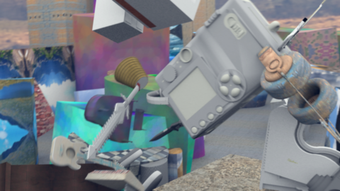
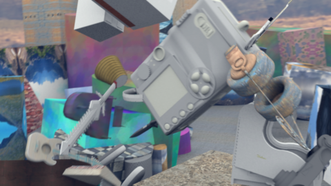
Left Image	Right Image
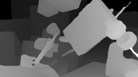
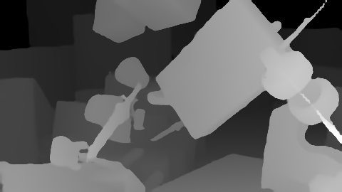
$\mathcal{L}_{log}$ Disparity	SEDNet Disparity
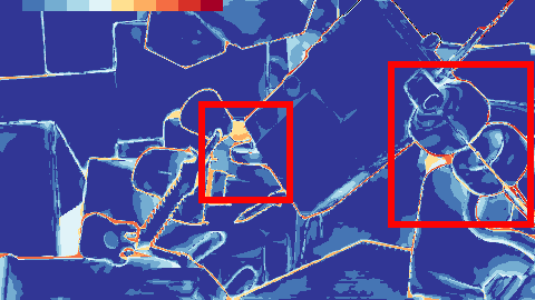
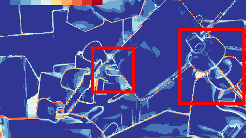
$\mathcal{L}_{log}$ Error	SEDNet Error
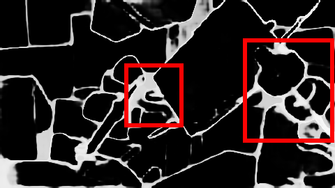
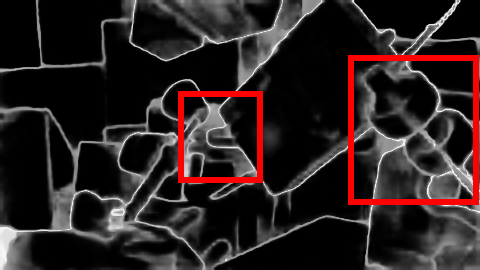
$\mathcal{L}_{log}$ Uncertainty	SEDNet Uncertainty

Figure S.2: Example from Scene Flow. When objects overlap with each other and depth ordering is unclear, SEDNet captures the uncertainty more precisely according to the error map. In the regions outlined in red, SEDNet successfully detects the pull ring of the camera and the lid of the wheel, while the $\mathcal{L}_{log}$ model fails to estimate their disparity.

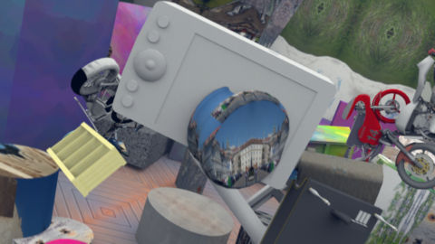
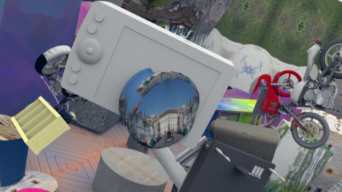
Left Image	Right Image
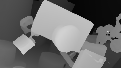
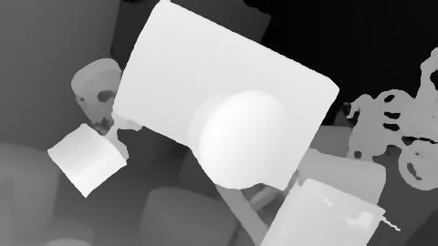
$\mathcal{L}_{log}$ Disparity	SEDNet Disparity
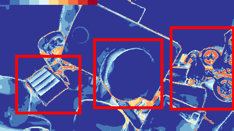
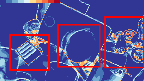
$\mathcal{L}_{log}$ Error	SEDNet Error
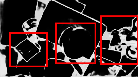
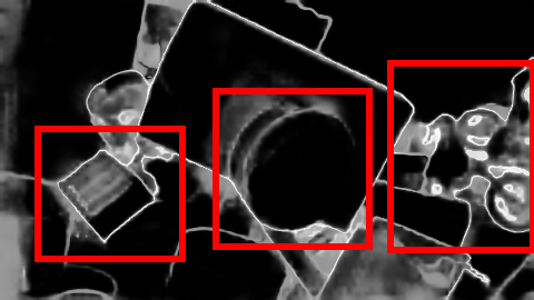
$\mathcal{L}_{log}$ Uncertainty	SEDNet Uncertainty

Figure S.3: Example from Scene Flow. The disparity and uncertainty maps of SEDNet include some structure information of the objects, such as the bookcase on the left side which has several openings, the cylinder which has many intersecting surfaces, and the wheels of the motorcycle. The prediction of $\mathcal{L}_{log}$ lacks these details.

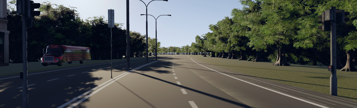
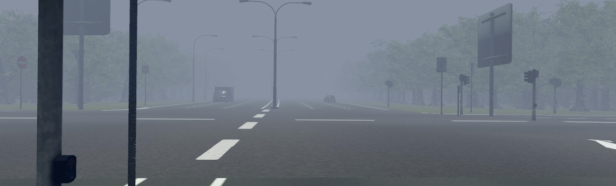
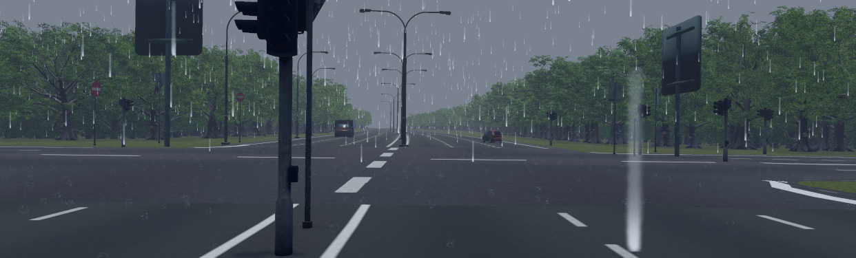
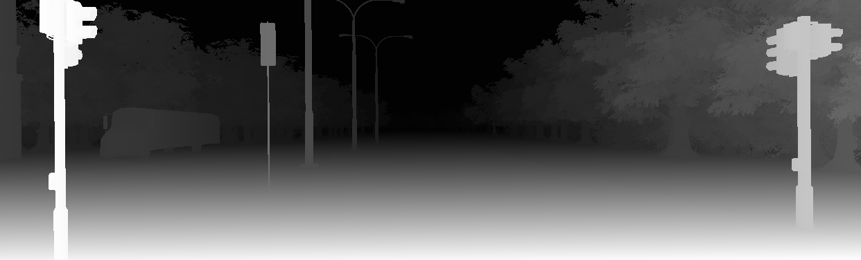
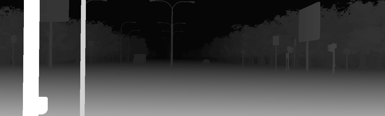
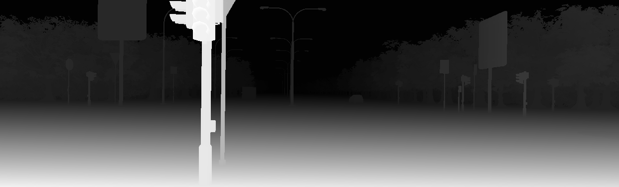
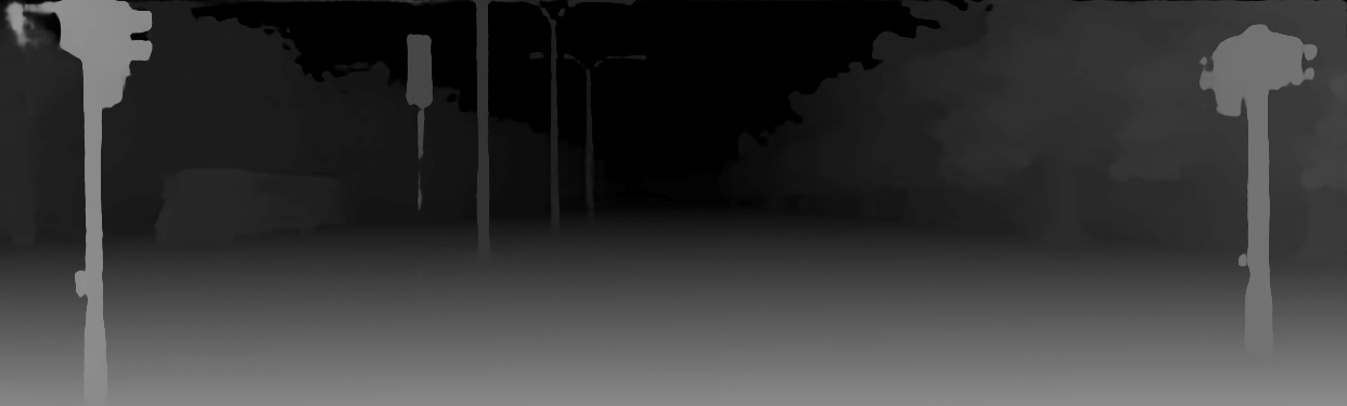
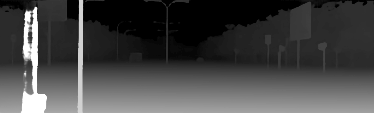
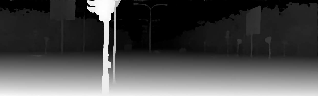
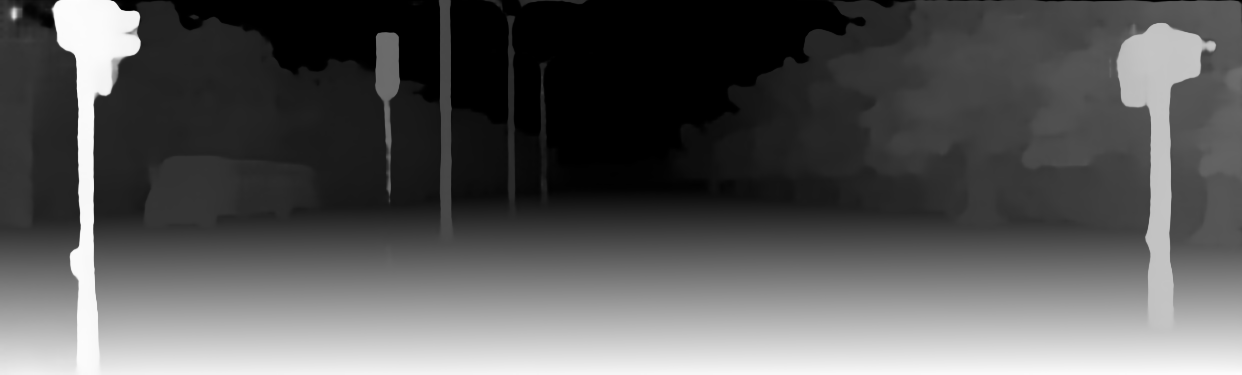
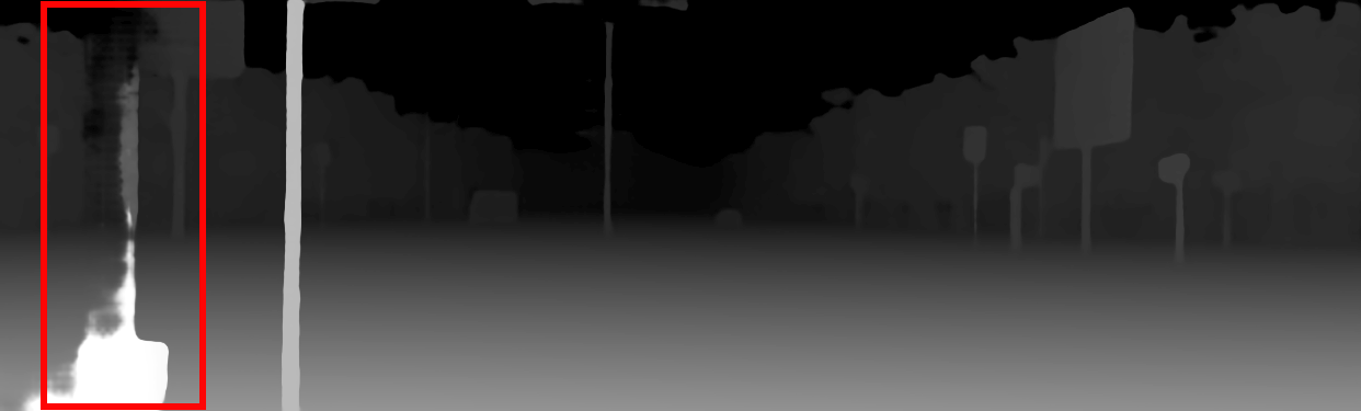
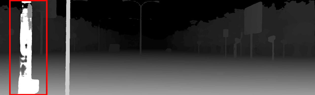
Sunny Foggy Rainy Left Images Ground Truth GwcNet $\mathcal{L}_{log}$ SEDNet

Figure S.4: Examples of driving in different weather conditions from VK2-S6. We pick the best $\mathcal{L}_{log}$ and SEDNet based on EPE in Table 1. (Please zoom in to see details.) SEDNet is better at predicting fine, challenging details in the disparity maps, such as the precise shape of the traffic light and the car under the left shadow in the sunny picture, the traffic sign behind the light post and the street light in the middle of the image in the fog.

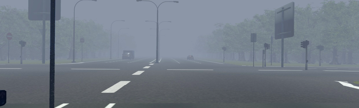
Left Image	Right Image
$\mathcal{L}_{log}$ Disparity	SEDNet Disparity
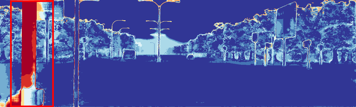
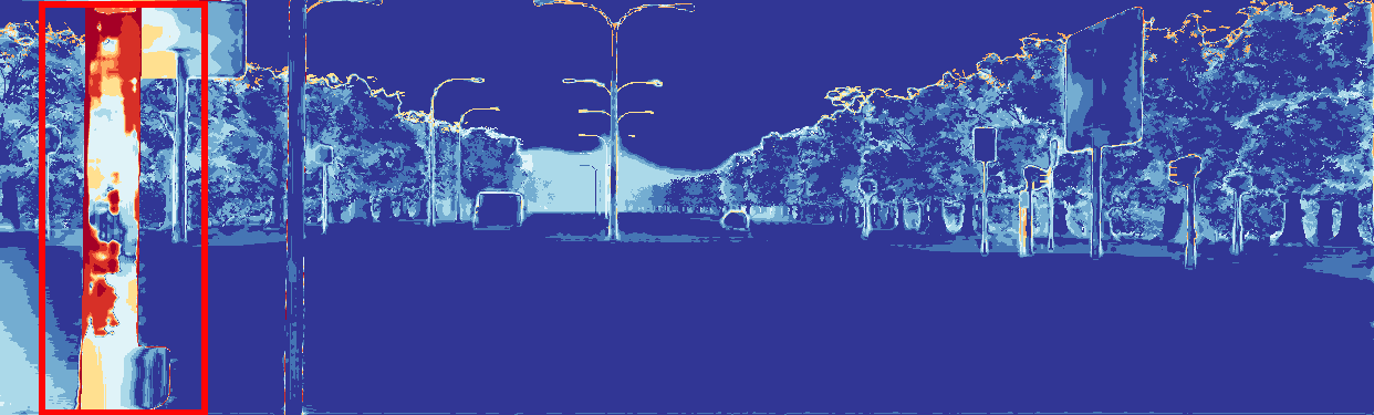
$\mathcal{L}_{log}$ Error	SEDNet Error
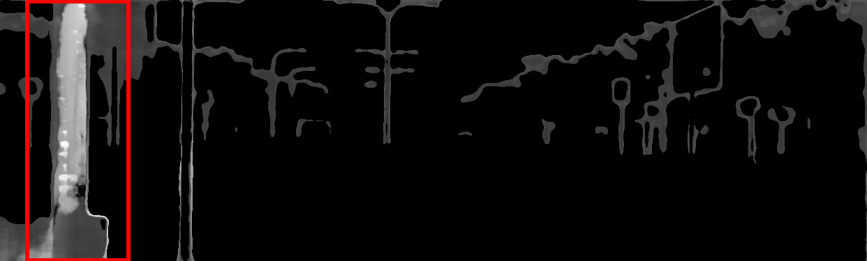
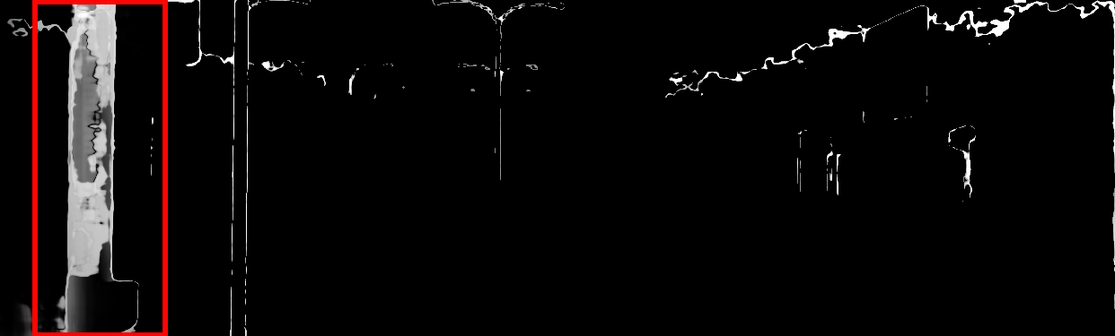
$\mathcal{L}_{log}$ Uncertainty	SEDNet Uncertainty

Figure S.5: Example from VK2-S6-Fog. The post only appears in the left image, $\mathcal{L}_{log}$ fails to predict its disparity, but SEDNet does. The uncertainty map of SEDNet matches the error map better than that of $\mathcal{L}_{log}$.

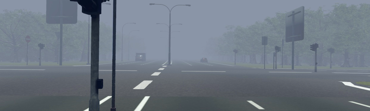
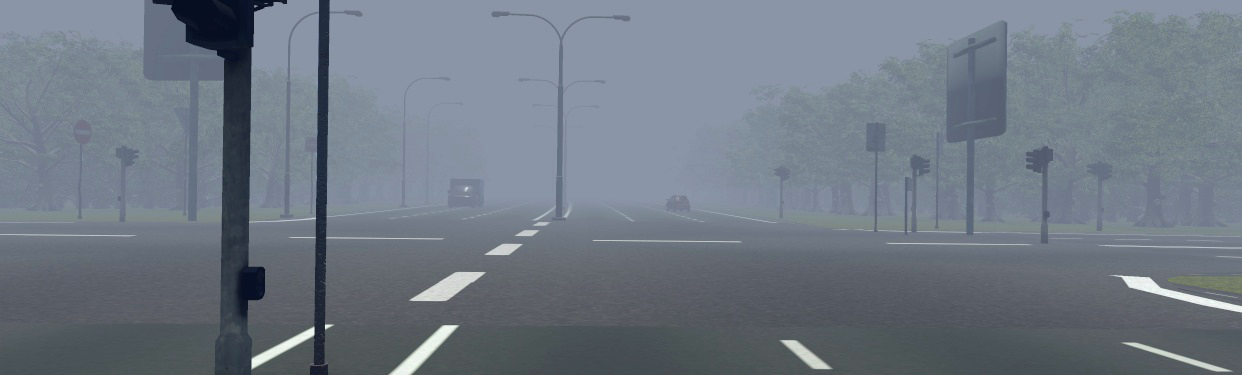
Left Image	Right Image
$\mathcal{L}_{log}$ Disparity	SEDNet Disparity
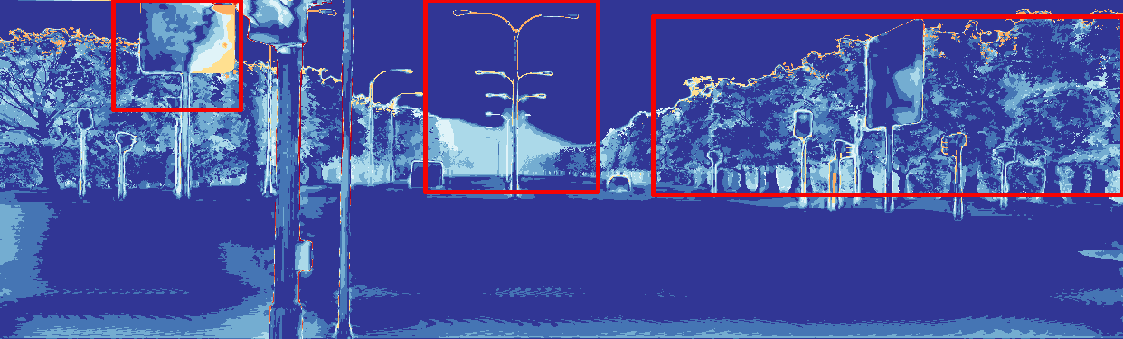
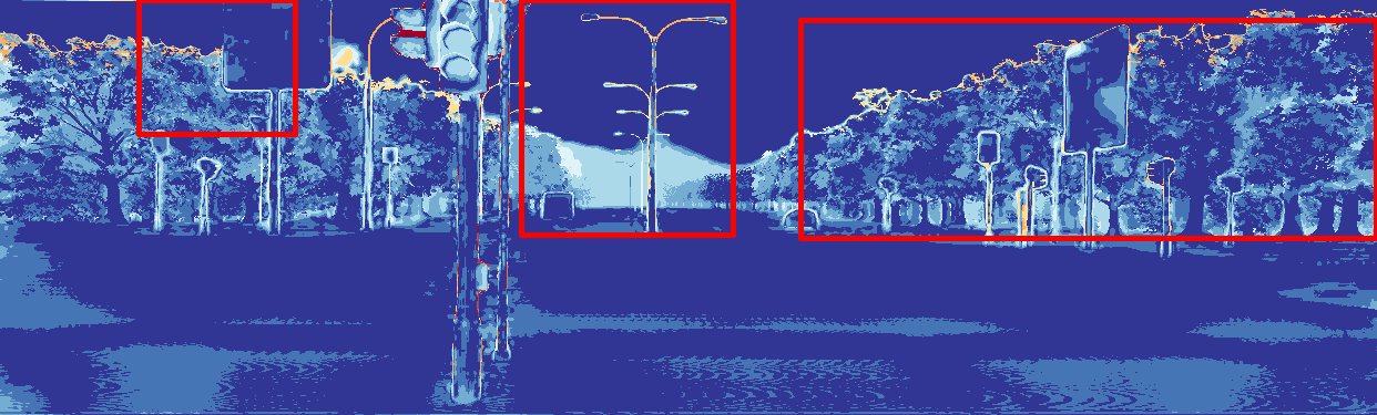
$\mathcal{L}_{log}$ Error	SEDNet Error
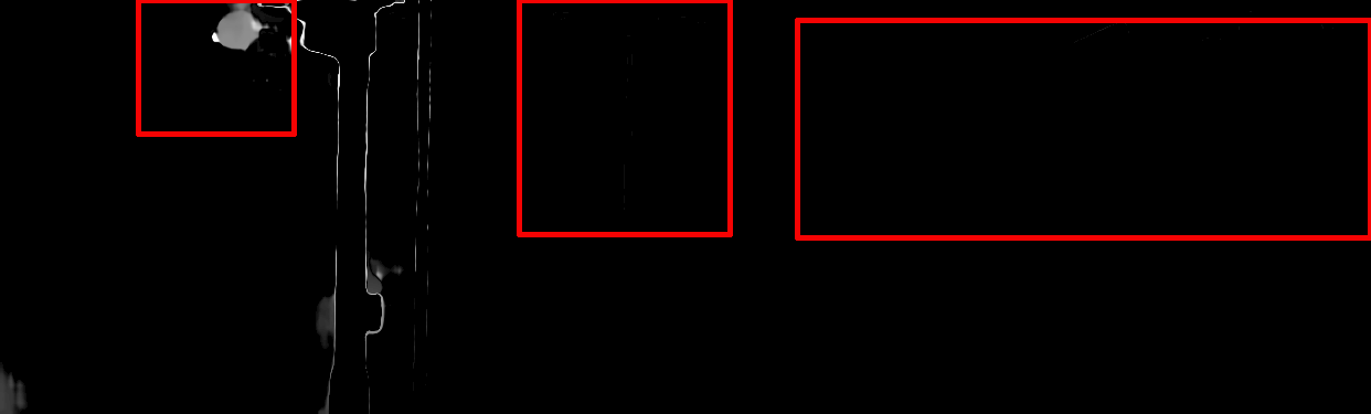
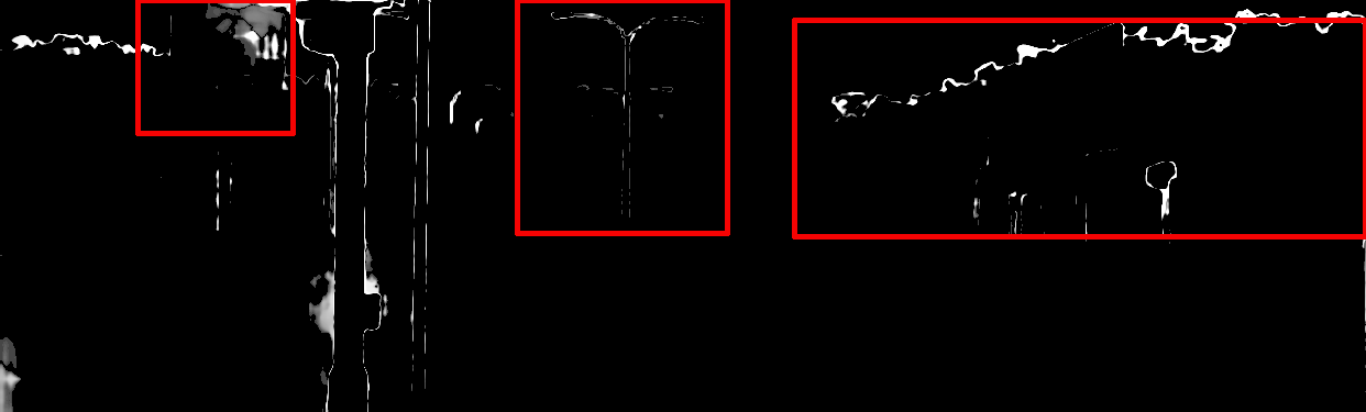
$\mathcal{L}_{log}$ Uncertainty	SEDNet Uncertainty

Figure S.6: Example from VK2-S6-Fog. Contrasting error and uncertainty maps, we observe that SEDNet predicts more accurate uncertainty in the regions covered by fog, such as the edges of the traffic signs and the trees in the background.

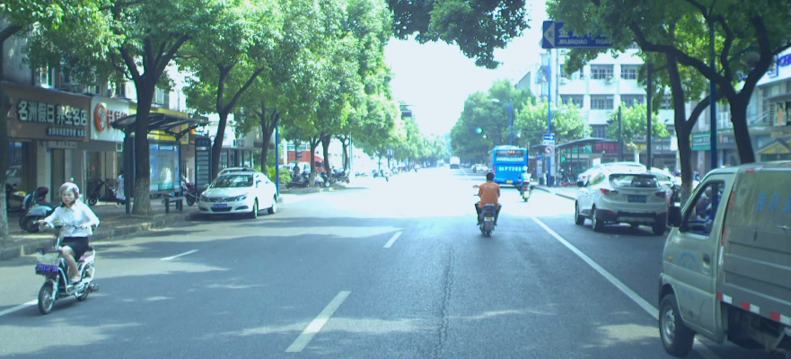
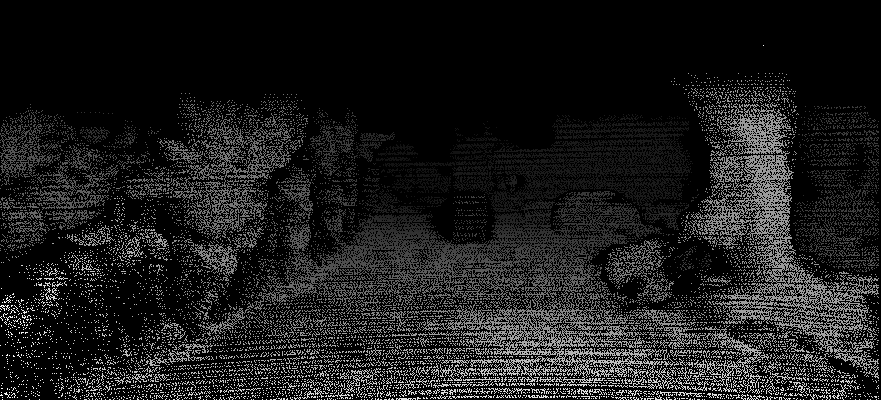
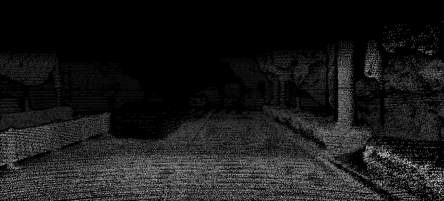
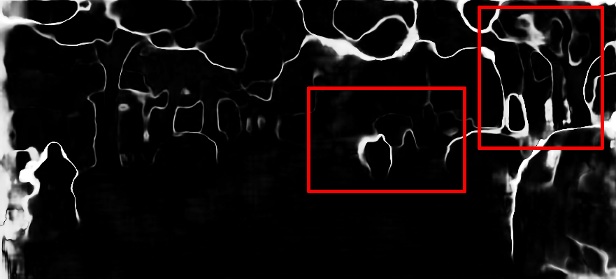
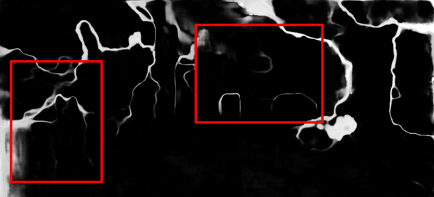
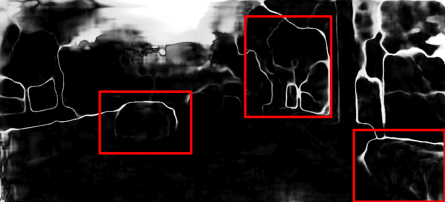
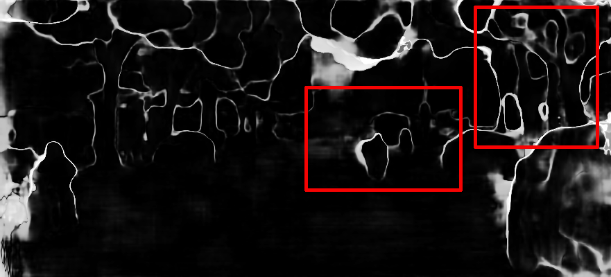
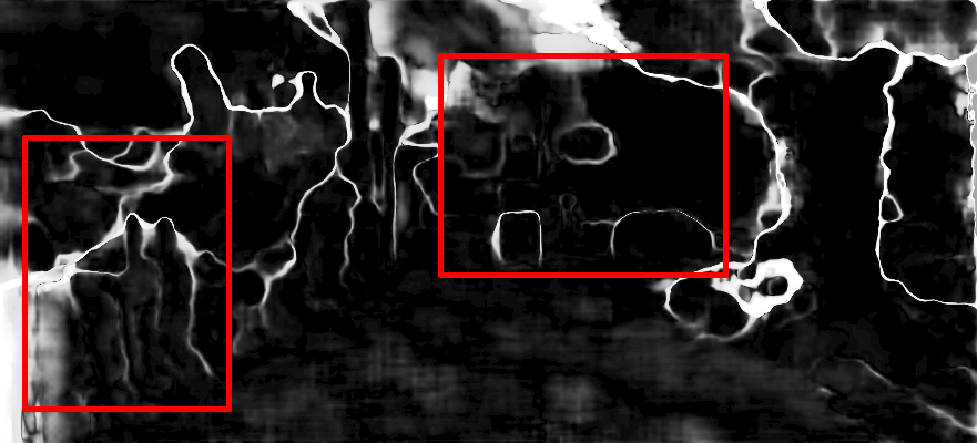
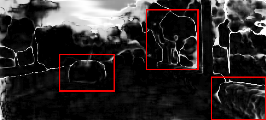
Left Image Ground Truth $\mathcal{L}_{log}$ SEDNet

Figure S.7: Examples of uncertainty estimation on DrivingStereo also shown in Table 1. SEDNet captures details more faithfully. For example, the cars, pedestrians and trees at different depths, even in overexposed parts of the images.

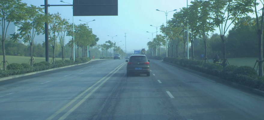
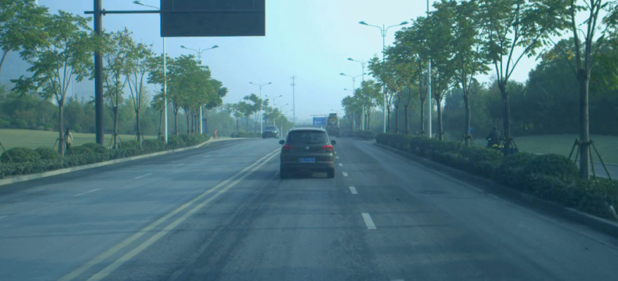
Left Image	Right Image
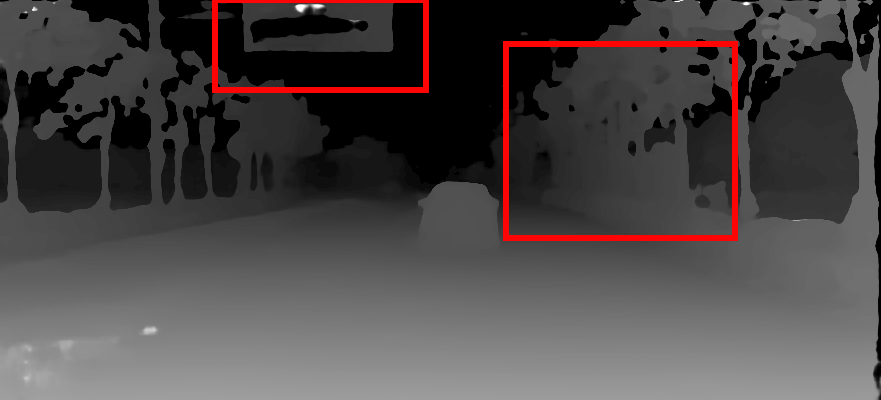
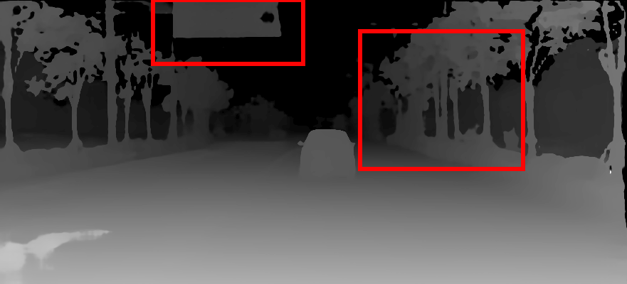
$\mathcal{L}_{log}$ Disparity	SEDNet Disparity
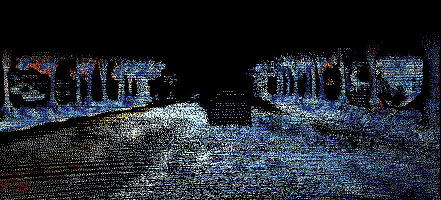
$\mathcal{L}_{log}$ Error	SEDNet Error
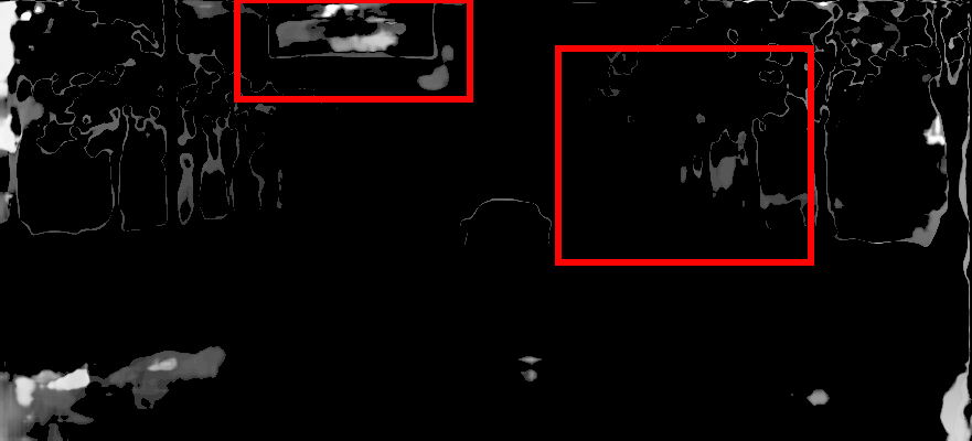
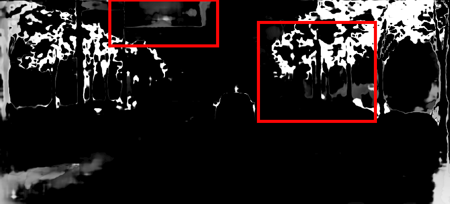
$\mathcal{L}_{log}$ Uncertainty	SEDNet Uncertainty

Figure S.8: Example from DS-Foggy. This subset is more challenging than the corresponding synthetic data due to unmodeled sources of noise. In this example, the thin tree trunk almost blends in with the background. Also, the billboard is very dark. $\mathcal{L}_{log}$ fails to predict the disparity of the textureless part of the billboard, as well as the space between the tree trunks on the right-hand side. The prediction of SEDNet is more accurate on these challenging parts.

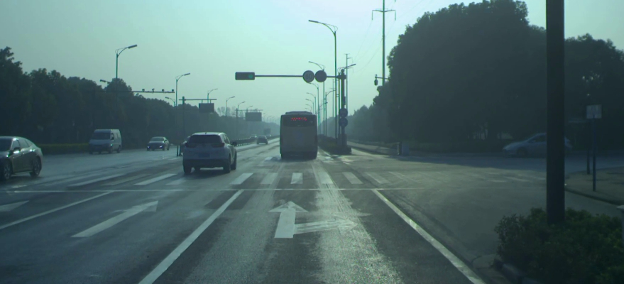
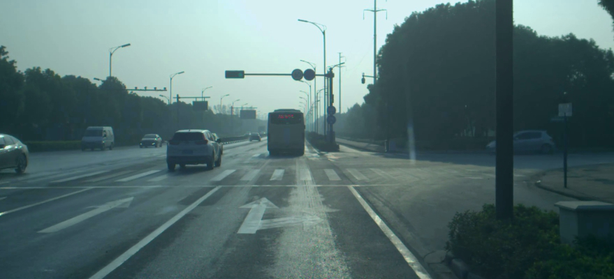
Left Image	Right Image
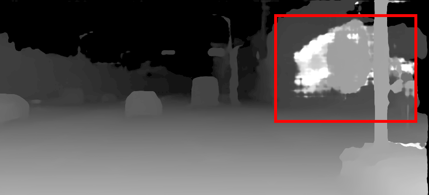
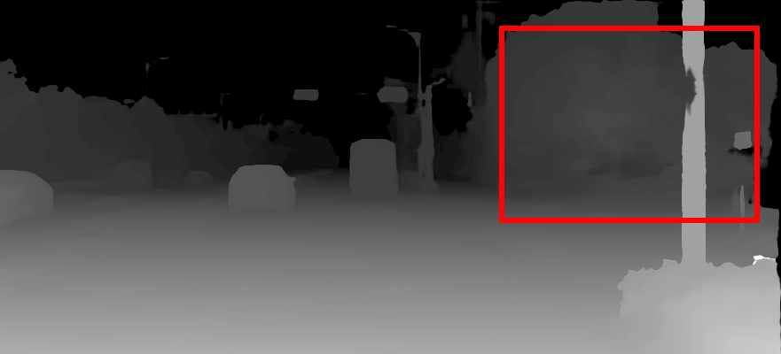
$\mathcal{L}_{log}$ Disparity	SEDNet Disparity
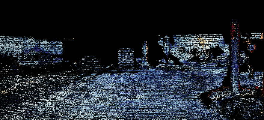
$\mathcal{L}_{log}$ Error	SEDNet Error
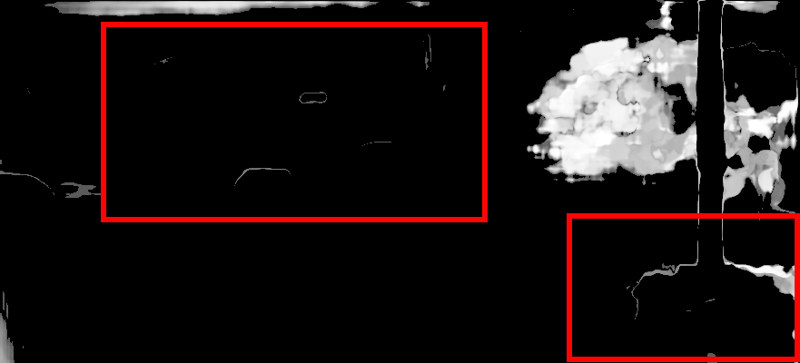
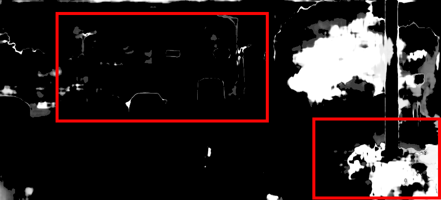
$\mathcal{L}_{log}$ Uncertainty	SEDNet Uncertainty

Figure S.9: Example from DS-Foggy. Similar to the synthetic data, images from the foggy day subset are usually very dark, which makes distinguishing objects in the shadow difficult. In this example, $\mathcal{L}_{log}$ makes a mistake in predicting the disparity of the trees on the right side, since they have similar color to the post. On the other hand, the prediction of SEDNet is more accurate. The uncertainty maps are dominated by the right backlit regions, making it hard to see the other parts. However, zooming in the figures reveals that SEDNet still performs better in predicting the uncertainty of the objects far from the camera and in the bottom right dark corner.

Left Image	Right Image
$\mathcal{L}_{log}$ Disparity	SEDNet Disparity
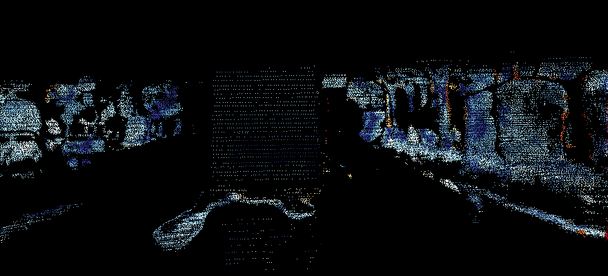
$\mathcal{L}_{log}$ Error	SEDNet Error
$\mathcal{L}_{log}$ Uncertainty	SEDNet Uncertainty

Figure S.10: Example from DS-Rainy. Unlike the synthetic data, the rainy-day real images do not only suffer from poor illumination, but also face challenges due to reflections in the water. In this example, the road is like a mirror, misleading the $\mathcal{L}_{log}$ model. Recall that the LIDAR ground truth disparity is very sparse, and is even sparser in reflective regions. Zooming in is required to see the recorded disparity errors on the road in the error maps. The disparity map of $\mathcal{L}_{log}$ fails to distinguish the car and the reflection, but SEDNet is able to estimate the correct disparity and the uncertainty of the car.

References

- [1] Charles Blundell, Julien Cornebise, Koray Kavukcuoglu, and Daan Wierstra. Weight uncertainty in neural network. In ICML, pages 1613–1622, 2015.
- [2] Jia-Ren Chang and Yong-Sheng Chen. Pyramid stereo matching network. In CVPR, pages 5410–5418, 2018.
- [3] Armen Der Kiureghian and Ove Ditlevsen. Aleatory or epistemic? does it matter? Structural safety, 31(2):105–112, 2009.
- [4] Zehua Fu, Mohsen Ardabilian, and Guillaume Stern. Stereo matching confidence learning based on multi-modal convolution neural networks. In International Workshop on Representations, Analysis and Recognition of Shape and Motion From Imaging Data, pages 69–81. Springer, 2017.
- [5] Zehua Fu and Mohsen Ardabilian Fard. Learning confidence measures by multi-modal convolutional neural networks. In WACV, pages 1321–1330, 2018.
- [6] Adrien Gaidon, Qiao Wang, Yohann Cabon, and Eleonora Vig. Virtual worlds as proxy for multi-object tracking analysis. In CVPR, pages 4340–4349, 2016.
- [7] Yarin Gal. Uncertainty in Deep Learning. PhD thesis, University of Cambridge, 2016.
- [8] Yarin Gal and Zoubin Ghahramani. Dropout as a bayesian approximation: Representing model uncertainty in deep learning. In ICML, pages 1050–1059, 2016.
- [9] Andreas Geiger, Philip Lenz, and Raquel Urtasun. Are we ready for autonomous driving? The KITTI vision benchmark suite. In CVPR, 2012.
- [10] Alex Graves. Practical variational inference for neural networks. In NeurIPS, volume 24, 2011.
- [11] Xiaoyang Guo, Kai Yang, Wukui Yang, Xiaogang Wang, and Hongsheng Li. Group-wise correlation stereo network. In CVPR, 2019.
- [12] Xiaoyan Hu and Philippos Mordohai. A quantitative evaluation of confidence measures for stereo vision. PAMI, 34(11):2121–2133, 2012.
- [13] Eddy Ilg, Ozgun Cicek, Silvio Galesso, Aaron Klein, Osama Makansi, Frank Hutter, and Thomas Brox. Uncertainty estimates and multi-hypotheses networks for optical flow. In ECCV, pages 652–667, 2018.
- [14] Alex Kendall and Yarin Gal. What uncertainties do we need in Bayesian deep learning for computer vision? In NeurIPS, pages 5574–5584, 2017.
- [15] Alex Kendall, Yarin Gal, and Roberto Cipolla. Multi-task learning using uncertainty to weigh losses for scene geometry and semantics. In CVPR, pages 7482–7491, 2018.
- [16] Alex Kendall, Hayk Martirosyan, Saumitro Dasgupta, Peter Henry, Ryan Kennedy, Abraham Bachrach, and Adam Bry. End-to-end learning of geometry and context for deep stereo regression. In ICCV, pages 66–75, 2017.
- [17] Sunok Kim, Seungryong Kim, Dongbo Min, Pascal Frossard, and Kwanghoon Sohn. Stereo confidence estimation via locally adaptive fusion and knowledge distillation. PAMI, 2022.
- [18] Sunok Kim, Seungryong Kim, Dongbo Min, and Kwanghoon Sohn. LAF-Net: Locally adaptive fusion networks for stereo confidence estimation. In CVPR, 2019.
- [19] Sunok Kim, Dongbo Min, Seungryong Kim, and Kwanghoon Sohn. Unified confidence estimation networks for robust stereo matching. TIP, 28(3):1299–1313, 2018.
- [20] Sunok Kim, Dongbo Min, Seungryong Kim, and Kwanghoon Sohn. Adversarial confidence estimation networks for robust stereo matching. TIST, 22(11):6875–6889, 2020.
- [21] Diederik P Kingma and Jimmy Ba. Adam: A method for stochastic optimization. arXiv preprint arXiv:1412.6980, 2014.
- [22] S Kullback and R Leibler. On information and sufficiencyannals of mathematical statistics, 22, 79–86. MathSciNet MATH, 1951.
- [23] Balaji Lakshminarayanan, Alexander Pritzel, and Charles Blundell. Simple and scalable predictive uncertainty estimation using deep ensembles. In NeurIPS, volume 30, 2017.
- [24] Zhengfa Liang, Yiliu Feng, Yulan Guo, Hengzhu Liu, Wei Chen, Linbo Qiao, Li Zhou, and Jianfeng Zhang. Learning for disparity estimation through feature constancy. In CVPR, pages 2811–2820, 2018.
- [25] Nikolaus Mayer, Eddy Ilg, Philip Hausser, Philipp Fischer, Daniel Cremers, Alexey Dosovitskiy, and Thomas Brox. A large dataset to train convolutional networks for disparity, optical flow, and scene flow estimation. In CVPR, pages 4040–4048, 2016.
- [26] Max Mehltretter. Joint estimation of depth and its uncertainty from stereo images using bayesian deep learning. ISPRS, 2:69–78, 2022.
- [27] Radford M Neal. Bayesian learning for neural networks, volume 118. Springer Science & Business Media, 2012.
- [28] David A Nix and Andreas S Weigend. Estimating the mean and variance of the target probability distribution. In ICNN, volume 1, pages 55–60. IEEE, 1994.
- [29] Matteo Poggi, Filippo Aleotti, Fabio Tosi, and Stefano Mattoccia. On the uncertainty of self-supervised monocular depth estimation. In CVPR, 2020.
- [30] Matteo Poggi, Seungryong Kim, Fabio Tosi, Sunok Kim, Filippo Aleotti, Dongbo Min, Kwanghoon Sohn, and Stefano Mattoccia. On the confidence of stereo matching in a deep-learning era: a quantitative evaluation. PAMI, 2021.
- [31] Matteo Poggi and Stefano Mattoccia. Learning from scratch a confidence measure. In BMVC, 2016.
- [32] Matteo Poggi, Fabio Tosi, Konstantinos Batsos, Philippos Mordohai, and Stefano Mattoccia. On the synergies between machine learning and binocular stereo for depth estimation from images: a survey. PAMI, 44(9):5314–5334, 2021.
- [33] Akihito Seki and Marc Pollefeys. Patch based confidence prediction for dense disparity map. In BMVC, pages 23.1–23.13, 2016.
- [34] Amit Shaked and Lior Wolf. Improved stereo matching with constant highway networks and reflective confidence learning. In CVPR, pages 4641–4650, 2017.
- [35] Fabio Tosi, Matteo Poggi, Antonio Benincasa, and Stefano Mattoccia. Beyond local reasoning for stereo confidence estimation with deep learning. In ECCV, pages 319–334, 2018.
- [36] Guorun Yang, Xiao Song, Chaoqin Huang, Zhidong Deng, Jianping Shi, and Bolei Zhou. DrivingStereo: A large-scale dataset for stereo matching in autonomous driving scenarios. In CVPR, 2019.
- [37] Guorun Yang, Xiao Song, Chaoqin Huang, Zhidong Deng, Jianping Shi, and Bolei Zhou. Drivingstereo: A large-scale dataset for stereo matching in autonomous driving scenarios. In CVPR, 2019.
- [38] Guorun Yang, Hengshuang Zhao, Jianping Shi, Zhidong Deng, and Jiaya Jia. SegStereo: Exploiting semantic information for disparity estimation. In ECCV, pages 636–651, 2018.
- [39] Feihu Zhang, Victor Prisacariu, Ruigang Yang, and Philip HS Torr. GA-Net: Guided aggregation net for end-to-end stereo matching. In CVPR, 2019.