Abstract

Recent developments in Machine Learning approaches for modelling physical systems have begun to mirror the past development of numerical methods in the computational sciences. In this survey we begin by providing an example of this with the parallels between the development trajectories of graph neural network acceleration for physical simulations and particle-based approaches. We then give an overview of simulation approaches, which have not yet found their way into state-of-the-art Machine Learning methods and hold the potential to make Machine Learning approaches more accurate and more efficient. We conclude by presenting an outlook on the potential of these approaches for making Machine Learning models for science more efficient.

1 Introduction

Recent years have seen an ever-larger push towards the application of Machine Learning to problems from the physical sciences such as Molecular Dynamics Musaelian et al. (2022b), coarse-graining Wang et al. (2022), the time-evolution of incompressible fluid flows Wang et al. (2020), learning governing equations from data Brunton et al. (2016); Cranmer et al. (2020), large-scale transformer models for chemistry Frey et al. (2022), and the acceleration of numerical simulations with machine learning techniques Kochkov et al. (2021). All of these algorithms build on the infrastructure underpinning modern Machine Learning in combing state-of-the-art approaches with a deep understanding of the physical problems at hand. This begs the questions if there exist more insights and tricks hidden in existing, classical approaches in the physical sciences which have the potential to maybe not only make the algorithm for the particular problem class more efficient, but maybe even Machine Learning in general?

Inspired by recent theoretical advances in the algorithmic alignment between Graph Neural Networks (GNNs) and dynamic programming Xu et al. (2020); Veličković et al. (2020), we surmise that the extension of this analysis to classical PDE solvers, and the physical considerations they incorporate, enables us to learn from the development trajectory in the physical sciences to inform the development of new algorithms. In this workshop paper we make the following contributions towards this goal:

• A comparison of the development of graph-based learned solvers, and the proximity of their development ideas to the development of Smoothed Particle Hydrodynamics starting from Molecular Dynamics in the physical sciences.

• An analysis of classical numerical solvers, and their algorithmic features to inform new ideas for new algorithms.

2 MeshGraphNets and its relation to classical methods

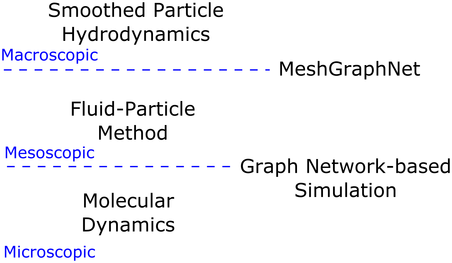
Figure 1: Characterization of the physical scales the example methods of section 2 operate on. The Graph Network-based approaches MeshGraphNets, and Graph Network-based Simulators are placed in relation to their classical counterparts.

An excellent example of the parallels between the development of Machine Learning methods for the sciences and the development of classical approaches is the recent development of graph-based simulators. When we relate their inherent assumptions and techniques to the development of particle-based methods, starting with Molecular Dynamics, a great many parallels arise. For an impression of the scales the classical methods operate on, and where graph-based simulators are placed in relation, please refer to Figure 1.

In this section, we analyze the structure of two of the first mature learned solvers (GNS Sanchez-Gonzalez et al. (2020), MeshGraphNets Pfaff et al. (2021)) and how these two approaches align with three of the classical methods (MD, FPM, SPH). We select these learned algorithms because they were one of the first of their kind to show promising results on real world data. Also, GNS is trained directly on SPH data which further motivates an algorithmic comparison.

2.1 Graph Neural Network-based Approaches to Simulation

The Graph Network (GN) Battaglia et al. (2018) is a framework that generalizes graph-based learning and specifically the Graph Neural Network (GNN) architecture by Scarselli et al. (2008). However, in this work, we use the terms GN and GNN interchangeably. Adopting the Graph Network formulation, the main design choices are the choice of update-function, and aggregation-function. For physics-informed modeling this gives us the ability to blur the line between classical methods and graph-based methods by including biases similar to CNNs for non-regular grids, as well as encoding physical laws into our network structure with the help of spatial equivariance/invariance, local interactions, the superposition principle, and differential equations. E.g. translational equivariance can easily be incorporated using relative positions between neighboring nodes, or the superposition principle can be encoded in graphs by using the summation aggregation over the representation of forces as edge features.

Viewing MeshGraphNets Pfaff et al. (2021) from a physics-motivated perspective, we argue that MeshGraphNets originate from Molecular Dynamics. To present this argument in all its clarity, we have to begin with its predecessor: the Graph Network-based Simulators (GNS) Sanchez-Gonzalez et al. (2020).

2.1.1 Graph Network-based Simulators

The Graph Networks-based Simulator builds on the encoder-processor-decoder approach, where Graph Networks are applied iteratively on the encoded space. Proving GNS’ ability to simulate systems with up to 85k particles, their approach can be summarized as follows.

Let $X^{t}$ denote the states of a particle system at time $t$. $X$ might contain the position, velocity, type of particle, or any other physical information specific to a material particle. A set of $k+1$ subsequent past states

$${\bf{X}}^{t_{0:K}}=\left\{X^{t_{0}},X^{t_{1}},\ldots,X^{t_{k}}\right\}$$

if given to the network. The core task is to then learn the differential operator $d_{\theta}$, which approximates the dynamics

$$d_{\theta}:X^{t_{k}}\longrightarrow Y^{t_{k}},\quad X^{t_{k+1}}=\text{Update}\left\{X^{t_{k}},d_{\theta}\right\}.$$

Here, $Y^{t}$ is the acceleration, which is used to obtain the next state $X^{t+1}$ via integration using a deterministic ”Update” routine, e.g. semi-implicit Euler scheme. The differential operator $d_{\theta}$ is learned with the encoder-processor-decoder approach where the encoder takes in 1 to 10 previous states, and encodes them into a graph. This graph consists of nodes - latent representation of the states $X$ - and edges - between each pair of particles closer than some cut-off radius there is another latent vector, which initially contains the distance or displacement information. The processor is then a multilayer Graph Network of which the exact number of message-passing Graph Networks is a hyperparameter. The result on the graph-space is then decoded back to physical space. The loss is computed as the mean-squared error between the learned acceleration, and the target acceleration. While the approach showed promising results for fluid simulations, and fluid-solid interactions, it struggled on deforming meshes, such as thin shells.

2.1.2 MeshGraphNets

To better represent meshes MeshGraphNets Pfaff et al. (2021) supplemented the Graph Network simulation with an additional set of edges to define a mesh, on which interactions can be learned. Closely related to the superposition principle in physics, the principle of splitting a complicated function into the sum of multiple simpler ones, the interaction function is split into the interaction of mesh-type edges and collision-type edges.

Following the widespread use of remeshing in engineering, MeshGraphNets have the ability to adaptively remesh to model a wider spectrum of dynamics. Mesh deformation without adaptive remeshing would lead to the loss of high frequency information.

The last major improvement of MeshGraphNets over GNS is extending the output vector $Y$ with additional components to also predict further targets, such as the stress field.

In difference to the Graph Network-based Simulators, the input here includes a predefined mesh and the output is extended to contain dynamical features like pressure.

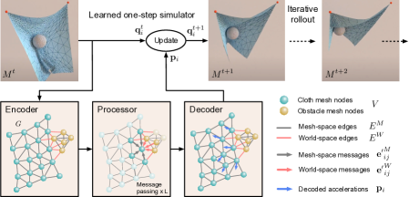
Figure 2: Illustration of the MeshGraphNets scheme with a decomposition of its algorithm into the encoder, processor, and decoder (Image source: Pfaff et al. (2021)).

2.2 Similarities between the Development Trajectories of Particle-based Methods and Graph Neural Network-based Approaches to Simulations

Beginning with Molecular Dynamics, the earliest and most fundamental particle-based method, we will now outline the similarities between the development trajectories, and the derivations inherent to them, of MeshGraphNets and the development of particle-based methods in physics.

2.2.1 Similarities to Molecular Dynamics

Molecular Dynamics is a widely used simulation method which generates the trajectories of an N-body atomic system. For the sake of intellectual clarity we restrict ourselves to its simplest form, the unconstrained Hamiltonian mechanics description.

The construction of connections, and edges is one of the clearest similarities between Molecular Dynamics and MeshGraphNets. Both can potentially have a mesh as an input, and both compute the interactions based on spatial distances up to a fixed threshold. Iterative updates, or the repeated application of Graph Network layers in the MeshGraphNets, extend the effective interaction radius beyond the immediate neighbourhood of a particle such that all particles can be interacted with. Both approaches are at the same time translationally invariant w.r.t. accelerations, and permutation equivariant w.r.t. the particles, and use a symplectic time-integrator. While there are theoretical reasons for this choice in Molecular Dynamics, it is choice of convenience in the context of learned approaches. The main difference between the two approaches lies in the computation of the accelerations. In Molecular Dynamics the derivative of a predefined potential function is evaluated, whereas a learned model is used in the Graph Network-based Simulators.

2.2.2 Similarities to Smoothed Particle Hydrodynamics

A closer relative to the Graph Network-based Simulators is the Smoothed Particle Hydrodynamics algorithm originating from astrophysics Lucy (1977); Gingold & Monaghan (1977). Smoothed Particle Hydrodynamics discretizes the governing equations of fluid dynamics, the Navier-Stokes equations, with kernels such that the discrete particles follow Newtonian mechanics with the equivalent of a prescribed molecular potential. Both, Smoothed Particle Hydrodynamics, and Graph Network-based Simulators obey the continuum assumption, whereas Molecular Dynamics presumes a discrete particle distribution, and is constrained to extremely short time intervals.

2.2.3 The Differences

Summarizing the key differences between the closely related approaches, Molecular Dynamics and Smoothed Particle Hydrodynamics both take one past state $X^{t}$ as an input, whereas Graph-based approaches require a history of $k$ states ${\bf{X}}^{t_{0:K}}$. Molecular Dynamics encodes geometric relations in the potential, MeshGraphNets encode the geometry in the mesh, while there exists no direct way for inclusion in the other two approaches. Molecular Dynamics, and Smoothed Particle Hydrodynamics explicitly encode physical laws, for learned methods all these parameters and relations have to be learned from data.

A key advancement of MeshGraphNets, coming from the Graph Network-based Simulators, is the explicit superimposition of solutions on both sets of edges, which far outperforms the implicit distinction of interactions. This approach is equally applicable to all conventional particle-, and mesh-based simulations in engineering. Borrowing the Fluid Particle Model from fluid mechanics, we can subsequently connect the classical methods with the learned approaches by viewing meshes and particles as the same entity under the fluid-particle paradigm.

2.2.4 Connecting MeshGraphNets to Graph Neural Network-based Simulations with the Fluid Particle Model

The Fluid Particle Model Espanol (1998) is a mesoscopic Newtonian model, as seen in Figure 1, situated on an intermediate scale between the microscopic Molecular Dynamics and the macroscopic Smoothed Particle Hydrodynamics. It views particles from the point of view of a Voronoi tesselation of the molecular fluid, see Figure 3. The Voronoi tesselation coarse-grains the atomistic system to a pseudoparticle system with ensembles of atoms in thermal equilibrium summarized as pseudoparticles. This pseudoparticle construction is closely related to the MeshGraphNets construction, where each mesh node also corresponds to the cell center of a simulated pseudoparticle. Smoothed Particle Hydrodynamics as well as Dissipative Particle Dynamics Hoogerbrugge & Koelman (1992) also both operate on pseudoparticles. All of these approaches share that they have to presume a large enough number of atoms per pseudoparticles to be viewed as a thermodynamic system.

Especially in Dissipative Particle Dynamics one injects Gaussian noise to approximate a physical system, just as is done for Graph Network-based Simulators and MeshGraphNets to stabilize the training. We surmise that this injection of noise into graph-based simulators amounts to forcing the learned model to predict the true output despite the noisy inputs, hence leading the model to converge to the central limit of the estimated conditional distribution of the acceleration.

The construction of Voronoi tesselations governs that the size of the cells is to be inversely proportional to variations in their properties, hence leading to more sampling in regions with high property variation. The very same argument based on the curvature as a heuristic is being used to derive the mesh refinement of the MeshGraphNets algorithm.

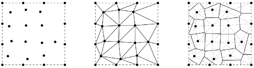
Figure 3: Single points (left), Delaunay triangulation (middle), and Voronoi diagram (right)(Image source: Rokicki & Gawell (2016)

3 Relation to Numerical Schemes

After the recent success of Neural ODEs solvers Chen et al. (2018), it has taken almost four years to start considering Neural PDEs in general Brandstetter et al. (2022). By definition, PDEs deal with derivatives of multiple variables, compared to ODEs having one variable. As a result, typical numerical approximations of PDEs are much more diverse depending on the peculiarities of the PDE of interest. Typical PDE solvers operating on grids (Eulerian description) include Finite Difference Methods (FDM), Finite Volume Methods (FVM), and Finite Element Methods (FEM), whereas other methods follow the trajectory of irregularly spaced points (Lagrangian description) like Smoothed Particle Hydrodynamics (SPH), Fluid Particle Model (FPM), Dissipative Particle Dynamics (DPD) Hoogerbrugge & Koelman (1992), Volume of Fluid Method (VOF) Hirt & Nichols (1981), Particle-in-Cell (PIC) Brackbill & Ruppel (1986), Material Point Method (MPM) Sulsky et al. (1993), Discrete Element Method (DEM) Cundall & Strack (1979), and Meshless FEM (MFEM). Finally, there are also approaches to solving PDEs without any discretization as in Sawhney et al. (2022). Each of these methods works best for a specific type of PDE, boundary/initial conditions, and parameter range. In this section we compare concepts from these classical methods to state-of-the-art learned algorithms.

3.1 Data augmentation with white noise

Two popular papers corrupting training inputs with additive Gaussian noise include Sanchez-Gonzalez et al. (2020); Pfaff et al. (2021), as described before. The goal of this approach is to force the model to deal with accumulating noise leading to a distribution shift during longer rollouts. Thus, the noise acts as an effective regularization technique, which in these two papers allows for much longer trajectories than seen during training. However, one major issue with this approach is that the scale of the noise is represented by two new hyperparameters, which have to be tuned manually (Pfaff et al. (2021), Appendix 2.2).

A perspective on noise injection coming from the physical sciences is to see it through the lens of mesoscopic particle methods like the Fluid Particle Model and Dissipative Particle Dynamics, in which the noise originates from the Brownian motion at small scales. Although GNS and MeshGraphNets operate on scales too large for the relevance of Brownian motion, the Fluid Particle Model provides a principled way of relating particle size and noise scale. The underlying considerations from statistical mechanics might aid to a better understanding of the influence of training noise and in turn make approaches based on it more efficient.

3.2 Data augmentation by multi-step loss

Another way of dealing with the distribution shift is by training a model to correct its own mistakes via some form of a multi-step loss, i.e. during training a short trajectory is generated and the loss is summed over one or multiple past steps Tompson et al. (2017); Um et al. (2020); Ummenhofer et al. (2020); Brandstetter et al. (2022). The results on this vary with some researchers reporting better performance than with noise injection Brandstetter et al. (2022), while others report the opposite experience Sanchez-Gonzalez et al. (2020).

Looking at classical solvers for something related to the multi-step loss, it is natural to think of adaptive time integrators used by default in ODE routines like ODE45 in Matlab Dormand & Prince (1980). Adaptive integrators work by generating two short trajectories of the same time length, but with different step sizes, and as long as the outcome with larger steps differs within some bounds, then the step size is increased. This guarantees some level of long-term rollout stability just as attempted with the multi-step loss, but the multi-step loss forces the network to implicitly correct for future deviations of the trajectory without actually changing the step size. The adaptive step-size idea has gained popularity in ML with the introduction of Neural ODEs Chen et al. (2018).

3.3 Equivariance bias

Numerical PDE solvers come in two flavors: stencil-based and kernel-based, both of which are equivariant to translation, rotation, and reflection in space (Euclidean group equivariance), as well as translation in time (by Noether’s theorem). These properties arise from the conservation of energy, which is a fundamental principle in physics. While equivariance, with respect to the Euclidean group, has been around for a couple of years on grids Weiler et al. (2018), its extension to the grid-free (Lagrangian) setting is gaining popularity just recently Brandstetter et al. (2021); Schütt et al. (2021); Batzner et al. (2022); Musaelian et al. (2022a). Here, we talk about equivariance in terms of a neural net operation on vectors, which rotates the output exactly the same way as the input is rotated, as opposed to working with scalar values, which is called an invariant operation, e.g. SchNet Schütt et al. (2017). The performance boost by including equivariant features is significant and reaches up to an order of magnitude compared to invariant methods Batzner et al. (2022).

3.4 Input multiple past steps

Another common performance improvement in neural net training is observed by stacking multiple past states as an input Sanchez-Gonzalez et al. (2020); Pfaff et al. (2021); Brandstetter et al. (2022). One argument supporting this approach is overfitting prevention by inputting more data Pfaff et al. (2021). Looking at conventional solvers we very rarely see multiple past states as input and this is done for materials with memory property, e.g. rheological fluids or ”smart” materials. Thus, providing multiple past states implicitly assumes that there is some nonphysical non-Markovian retardation process, which in most cases does not correspond to the physics used for training data generated.

The only physical justification of a multi-step input we are aware of arises if we train the model to learn a coarse-grained representation of the system. Li et al. (2015) showed that explicit memory effects are necessary in Dissipative Particle Dynamics for the correct coarse-graining of a complex dynamical system using the Mori-Zwanzig formalism. Given that papers like GNS and MeshGraphNets do not make use of coarse-graining, it is questionable why we observe improvement in performance and whether this trick generalizes well to different settings.

3.5 Spatial multi-scale modeling

Conventional multi-scale methods include, among others, all types of coarse-graining, Wavelet-based methods (e.g. Kim et al. (2008)), and the Fast Multipole Method Rokhlin (1985). Graph Networks seem especially suitable for tasks like coarse-graining as they are designed to work on unstructured domains, opposed for example to approaches using Wavelet or Fourier transforms, which require regular grids. GNNs seem especially promising with many applications in Molecular Dynamics Husic et al. (2020) and engineering Lino et al. (2021); Valencia et al. (2022); Migus et al. (2022); Han et al. (2022). It is particularly interesting to see works like Migus et al. (2022) inspired by multi-resolution methods and Valencia et al. (2022) resembling geometric coarse-graining by weighted averaging. All these methods rely on the fact that physical systems exhibit multi-scale behavior, meaning that the trajectory of a particle depends on its closest neighbors, but also on more far-reaching weaker forces. Splitting the scales and combining their contributions can greatly reduce computation. One of the great advantages of GNNs is their capability to operate on irregularly spaced data, which is necessary for most coarse-graining approaches.

3.6 Locality of interactions

In most cases, graph-based approaches to solving PDEs define the edges in the graph, based on an interaction radius. Methods using the Graph Network architecture Battaglia et al. (2018) effectively expand the receptive field of each node with every further layer, in the extreme case resulting in the phenomenon known as over-smoothing. But if we keep the number of layers reasonably low, the receptive field will always be larger compared to a conventional simulation with the same radius. Until recently, it was thought that a large receptive field is the reason for the success of learned simulators, but Musaelian et al. (2022a) question that assumption. In this paper, an equivariant graph network with fixed interaction neighbors performs on a par with the very similar Graph Network-based method NequIP Batzner et al. (2022) on molecular property prediction tasks. This finding supports the physics-based argument about the locality of interactions.

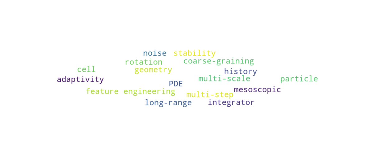
Figure 4: Overview of the currently under-utilized ideas discussed in Section 4 for Machine Learning approaches for the physical sciences.

3.7 Mesh vs Particle

GNN-based simulation approaches offer the flexibility to combine particles and meshes out-of-the-box. If we then train one neural network to reproduce the results of a Finite Element solution on a mesh and Smoothed Particle Hydrodynamics solution over particles, this is where learned methods really shine. This was achieved with the MeshGraphNets framework Pfaff et al. (2021). We argue that the transition from particles to meshes is a direct result of a coarse-graining procedure using Voronoi tessellation, which is related to the derivation of the Fluid Particle Model. The main assumption in this derivation is that each mesh cell should be small enough that it can be treated as being in equilibrium - similar to the assumption made when discretizing a domain with points.

3.8 Stencils

We talk about stencils when operating on regular grids. Although this is not the main strength of GNNs, there are some useful concepts from stencil-based simulations, which are conventionally nontrivial to generalize to particles, but can easily be adapted with GNNs. Brandstetter et al. (2022) state that their paper is motivated by the observation that the Weighted Essentially Non-Oscillatory scheme (WENO) Shu (1998) can be written as a special case of a GNN. Another work, inspired by the general idea of the Finite Volume Method, looking at the fluxes at the left and right cell boundary, was developed by Praditia et al. (2021). Inspired by the Finite Element Method, finite element networks were introduced by weighting the contributions of neighbouring cells by their volume, as is done in Finite Element analysis Lienen & Günnemann (2022).

3.9 Integration schemes

In addition to the time-step adaptation mentioned in relation to multi-step losses, another topic investigated in literature is the order of the integrator Sanchez-Gonzalez et al. (2019). This work points to the fact that higher order integrators lead to much better robustness, with respect to the choice of an integration time step. Another interesting question discussed in this paper is whether symplectic integrators improve performance of a learned Hamiltonian neural net. The answer seems to be that the symplectic property is much less important than the order of the integrator, which is in contrast with conventional Molecular Dynamics integrators, which work extremely poorly if not symplectic.

4 Untapped Ideas from Classical Approaches

In this subsection, we introduce potentially useful ideas from conventional differential equation solvers in science, which to the best of our knowledge have not been adapted in main-stream learned PDE solvers yet. Figure 4 is a collection of these concepts in the form of a word cloud.

4.1 Noise during inference

Adding noise to the inputs during training has proven to be useful, but has not been done during testing. One idea would be to use noise during inference to emulate Brownian motion. And one further topic we already mentioned is the relation of the noise scale to particle mass. From mesoscopic methods and the Fluctuation-dissipation theorem we would expect the noise to scale as $1/\sqrt{m}$ if a coarser representation is used.

4.2 Multiple time steps

Learned Molecular Dynamics simulations stick to using only the last past state and doing the same for larger-scale simulations might partially explain the unphysical behavior of the GNS method demonstrated in Klimesch et al. (2022). For coarse-graining though a longer history might be helpful.

4.3 Feature Engineering

From the Volume of Fluid Method we could adapt the idea of including features corresponding to the ratio of different material, if we are interested in simulating multi-material flows. The Discrete Element Method suggests encoding much more features like rotational degree of freedom (in magnetic field or simulating friction), stateful contact information (contact simulations), and often complicated geometry (for non-spherical, e.g. granular particles). Inspired by shock-capturing methods used routinely for the solution of nonlinear fluid dynamics problems Ketcheson et al. (2020), one could think of further hand-tuned node features indicating the presence of a shock.

4.4 Particles and Grid

There are a number of methods using the best of both particle and grid worlds like the Particle-in-Cell method and its successor Material Point Method. The idea of updating the node features and from time to time also based on the grid cell they belong to, might speed up simulations and is worth exploring. Now, if we restrict ourselves to regularly spaced particles, respectively grid cells, our solver toolkit becomes much richer with methods like the Fast Fourier Transform (which has already seen great success with the Fourier Neural Operator Li et al. (2020)) and the Wavelet Transform (as used in the PDE-Net Long et al. (2018)) at our disposal, as mentioned above in the context of multi-scale modeling.

4.5 Integrator

Taking the perspective of Neural ODEs Chen et al. (2018) with the neural network learning the perfect acceleration, one could arguably expect the next evolutionary step to be the combination of learned integrators with adaptive integration schemes. Incorporating insights from classical numerical methods, one should possibly seek to define an equivalent stability criterion for learned methods as the Courant-Friedrichs-Lewy (CFL) condition for classical numerical methods. This would in turn aid in bounding the time, and subsequently explore time steps smaller than the critical value.

5 Conclusion & Discussion

In this article, we claim that studying classical PDE solvers and their past development offers a direct path to the acceleration of the development of learned PDE solvers. Examples in literature show that biasing a learned solver by means of architectural design, data augmentation, feature engineering, etc. incorporating existing knowledge from classical solvers can greatly improve performance, explainability, and data-efficiency.

In Section 2 we show how this development has already subconsciously played out in the development of graph-based learned solvers following the same development as particle-based methods such as Molecular Dynamics, Smoothed Particle Hydrodynamics, and the Fluid-Particle Model. This investigation is revisited for algorithmic comparisons and illustrations of the limitations of classical solvers later on. In Section 3 we then focus on ideas from classical approaches which have found their way into recent learned solver literature, and discuss the physical interpretation of these developments. In the discussed examples, the included physically motivated biases are used to improve robustness w.r.t. hyperparameter choices, lower errors, and speed-up inference.

Section 4 takes a glimpse into a possible version of the future with ideas which have, to the best of our knowledge, not yet been integrated in learned methods. Given the elaborate history of classical methods, and the short, but highly dynamic history of learned approaches, there is still a lot of potential to be realized within the latter by incorporating insights from the former.

Going further, many exciting problems in the physical sciences, such as simulations involving multiple spatial scales, multiple temporal scales, non-Newtonian fluids, or phase-changing materials, are heavily data-constrained and will hence have to rely on insights from classical methods for Machine Learning approaches to become feasible.

References

- Battaglia et al. (2018) Battaglia, P. W., Hamrick, J. B., Bapst, V., Sanchez-Gonzalez, A., Zambaldi, V., Malinowski, M., Tacchetti, A., Raposo, D., Santoro, A., Faulkner, R., et al. Relational inductive biases, deep learning, and graph networks. arXiv preprint arXiv:1806.01261, 2018.
- Batzner et al. (2022) Batzner, S., Musaelian, A., Sun, L., Geiger, M., Mailoa, J. P., Kornbluth, M., Molinari, N., Smidt, T. E., and Kozinsky, B. E (3)-equivariant graph neural networks for data-efficient and accurate interatomic potentials. Nature communications, 13(1):1–11, 2022.
- Brackbill & Ruppel (1986) Brackbill, J. U. and Ruppel, H. M. Flip: A method for adaptively zoned, particle-in-cell calculations of fluid flows in two dimensions. Journal of Computational physics, 65(2):314–343, 1986.
- Brandstetter et al. (2021) Brandstetter, J., Hesselink, R., van der Pol, E., Bekkers, E., and Welling, M. Geometric and physical quantities improve e (3) equivariant message passing. arXiv preprint arXiv:2110.02905, 2021.
- Brandstetter et al. (2022) Brandstetter, J., Worrall, D. E., and Welling, M. Message passing neural PDE solvers. In International Conference on Learning Representations, 2022.
- Brunton et al. (2016) Brunton, S. L., Proctor, J. L., and Kutz, J. N. Discovering governing equations from data by sparse identification of nonlinear dynamical systems. Proceedings of the national academy of sciences, 113(15):3932–3937, 2016.
- Chen et al. (2018) Chen, R. T. Q., Rubanova, Y., Bettencourt, J., and Duvenaud, D. K. Neural ordinary differential equations. In Bengio, S., Wallach, H., Larochelle, H., Grauman, K., Cesa-Bianchi, N., and Garnett, R. (eds.), Advances in Neural Information Processing Systems, volume 31. Curran Associates, Inc., 2018.
- Cranmer et al. (2020) Cranmer, M., Sanchez Gonzalez, A., Battaglia, P., Xu, R., Cranmer, K., Spergel, D., and Ho, S. Discovering symbolic models from deep learning with inductive biases. Advances in Neural Information Processing Systems, 33:17429–17442, 2020.
- Cundall & Strack (1979) Cundall, P. A. and Strack, O. D. A discrete numerical model for granular assemblies. geotechnique, 29(1):47–65, 1979.
- Dormand & Prince (1980) Dormand, J. R. and Prince, P. J. A family of embedded runge-kutta formulae. Journal of computational and applied mathematics, 6(1):19–26, 1980.
- Espanol (1998) Espanol, P. Fluid particle model. Physical Review E, 57(3):2930, 1998.
- Frey et al. (2022) Frey, N., Soklaski, R., Axelrod, S., Samsi, S., Gomez-Bombarelli, R., Coley, C., and Gadepally, V. Neural scaling of deep chemical models. 2022.
- Gingold & Monaghan (1977) Gingold, R. A. and Monaghan, J. J. Smoothed particle hydrodynamics: theory and application to non-spherical stars. Monthly notices of the royal astronomical society, 181(3):375–389, 1977.
- Han et al. (2022) Han, X., Gao, H., Pfaff, T., Wang, J.-X., and Liu, L. Predicting physics in mesh-reduced space with temporal attention. In International Conference on Learning Representations, 2022.
- Hirt & Nichols (1981) Hirt, C. W. and Nichols, B. D. Volume of fluid (vof) method for the dynamics of free boundaries. Journal of computational physics, 39(1):201–225, 1981.
- Hoogerbrugge & Koelman (1992) Hoogerbrugge, P. and Koelman, J. Simulating microscopic hydrodynamic phenomena with dissipative particle dynamics. EPL (Europhysics Letters), 19(3):155, 1992.
- Husic et al. (2020) Husic, B. E., Charron, N. E., Lemm, D., Wang, J., Pérez, A., Majewski, M., Krämer, A., Chen, Y., Olsson, S., de Fabritiis, G., et al. Coarse graining molecular dynamics with graph neural networks. The Journal of chemical physics, 153(19):194101, 2020.
- Ketcheson et al. (2020) Ketcheson, D. I., LeVeque, R. J., and del Razo, M. J. Riemann Problems and Jupyter Solutions. Society for Industrial and Applied Mathematics, Philadelphia, PA, 2020. doi: 10.1137/1.9781611976212.
- Kim et al. (2008) Kim, T., Thürey, N., James, D., and Gross, M. Wavelet turbulence for fluid simulation. ACM Transactions on Graphics (TOG), 27(3):1–6, 2008.
- Klimesch et al. (2022) Klimesch, J., Holl, P., and Thuerey, N. Simulating liquids with graph networks. arXiv preprint arXiv:2203.07895, 2022.
- Kochkov et al. (2021) Kochkov, D., Smith, J. A., Alieva, A., Wang, Q., Brenner, M. P., and Hoyer, S. Machine learning–accelerated computational fluid dynamics. Proceedings of the National Academy of Sciences, 118(21), 2021.
- Li et al. (2015) Li, Z., Bian, X., Li, X., and Karniadakis, G. E. Incorporation of memory effects in coarse-grained modeling via the mori-zwanzig formalism. The Journal of chemical physics, 143(24):243128, 2015.
- Li et al. (2020) Li, Z., Kovachki, N., Azizzadenesheli, K., Liu, B., Bhattacharya, K., Stuart, A., and Anandkumar, A. Fourier neural operator for parametric partial differential equations. arXiv preprint arXiv:2010.08895, 2020.
- Lienen & Günnemann (2022) Lienen, M. and Günnemann, S. Learning the dynamics of physical systems from sparse observations with finite element networks. In International Conference on Learning Representations (ICLR), 2022.
- Lino et al. (2021) Lino, M., Cantwell, C., Bharath, A. A., and Fotiadis, S. Simulating continuum mechanics with multi-scale graph neural networks. arXiv preprint arXiv:2106.04900, 2021.
- Long et al. (2018) Long, Z., Lu, Y., Ma, X., and Dong, B. Pde-net: Learning pdes from data. In International Conference on Machine Learning, pp. 3208–3216. PMLR, 2018.
- Lucy (1977) Lucy, L. B. A numerical approach to the testing of the fission hypothesis. The astronomical journal, 82:1013–1024, 1977.
- Migus et al. (2022) Migus, L., Yin, Y., Mazari, J. A., and patrick gallinari. Multi-scale physical representations for approximating PDE solutions with graph neural operators. In ICLR 2022 Workshop on Geometrical and Topological Representation Learning, 2022.
- Musaelian et al. (2022a) Musaelian, A., Batzner, S., Johansson, A., Sun, L., Owen, C. J., Kornbluth, M., and Kozinsky, B. Learning local equivariant representations for large-scale atomistic dynamics, 2022a.
- Musaelian et al. (2022b) Musaelian, A., Batzner, S., Johansson, A., Sun, L., Owen, C. J., Kornbluth, M., and Kozinsky, B. Learning local equivariant representations for large-scale atomistic dynamics. arXiv preprint arXiv:2204.05249, 2022b.
- Pfaff et al. (2021) Pfaff, T., Fortunato, M., Sanchez-Gonzalez, A., and Battaglia, P. Learning mesh-based simulation with graph networks. In International Conference on Learning Representations, 2021.
- Praditia et al. (2021) Praditia, T., Karlbauer, M., Otte, S., Oladyshkin, S., Butz, M. V., and Nowak, W. Finite volume neural network : Modeling subsurface contaminant transport. In ICLR 2021 : Ninth International Conference on Learning Representations. Cornell University, 2021. doi: 10.48550/arXiv.2104.06010.
- Rokhlin (1985) Rokhlin, V. Rapid solution of integral equations of classical potential theory. Journal of computational physics, 60(2):187–207, 1985.
- Rokicki & Gawell (2016) Rokicki, W. and Gawell, E. Voronoi diagrams–architectural and structural rod structure research model optimization. MAZOWSZE Studia Regionalne, (19):155–164, 2016.
- Sanchez-Gonzalez et al. (2019) Sanchez-Gonzalez, A., Bapst, V., Cranmer, K., and Battaglia, P. Hamiltonian graph networks with ode integrators. arXiv preprint arXiv:1909.12790, 2019.
- Sanchez-Gonzalez et al. (2020) Sanchez-Gonzalez, A., Godwin, J., Pfaff, T., Ying, R., Leskovec, J., and Battaglia, P. Learning to simulate complex physics with graph networks. In International Conference on Machine Learning, pp. 8459–8468. PMLR, 2020.
- Sawhney et al. (2022) Sawhney, R., Seyb, D., Jarosz, W., and Crane, K. Grid-free Monte Carlo for PDEs with spatially varying coefficients. ACM Transactions on Graphics (Proceedings of SIGGRAPH), 41(4), July 2022. doi: 10.1145/3528223.3530134.
- Scarselli et al. (2008) Scarselli, F., Gori, M., Tsoi, A. C., Hagenbuchner, M., and Monfardini, G. The graph neural network model. IEEE transactions on neural networks, 20(1):61–80, 2008.
- Schütt et al. (2017) Schütt, K., Kindermans, P.-J., Sauceda Felix, H. E., Chmiela, S., Tkatchenko, A., and Müller, K.-R. Schnet: A continuous-filter convolutional neural network for modeling quantum interactions. Advances in neural information processing systems, 30, 2017.
- Schütt et al. (2021) Schütt, K., Unke, O., and Gastegger, M. Equivariant message passing for the prediction of tensorial properties and molecular spectra. In Meila, M. and Zhang, T. (eds.), Proceedings of the 38th International Conference on Machine Learning, volume 139 of Proceedings of Machine Learning Research, pp. 9377–9388. PMLR, 18–24 Jul 2021.
- Shu (1998) Shu, C.-W. Essentially non-oscillatory and weighted essentially non-oscillatory schemes for hyperbolic conservation laws. In Advanced numerical approximation of nonlinear hyperbolic equations, pp. 325–432. Springer, 1998.
- Sulsky et al. (1993) Sulsky, D., Chen, Z., and Schreyer, H. L. A particle method for history-dependent materials. Technical report, Sandia National Labs., Albuquerque, NM (United States), 1993.
- Tompson et al. (2017) Tompson, J., Schlachter, K., Sprechmann, P., and Perlin, K. Accelerating Eulerian fluid simulation with convolutional networks. In Precup, D. and Teh, Y. W. (eds.), Proceedings of the 34th International Conference on Machine Learning, volume 70 of Proceedings of Machine Learning Research, pp. 3424–3433. PMLR, 06–11 Aug 2017.
- Um et al. (2020) Um, K., Brand, R., Fei, Y. R., Holl, P., and Thuerey, N. Solver-in-the-loop: Learning from differentiable physics to interact with iterative pde-solvers. In Larochelle, H., Ranzato, M., Hadsell, R., Balcan, M., and Lin, H. (eds.), Advances in Neural Information Processing Systems, volume 33, pp. 6111–6122. Curran Associates, Inc., 2020.
- Ummenhofer et al. (2020) Ummenhofer, B., Prantl, L., Thuerey, N., and Koltun, V. Lagrangian fluid simulation with continuous convolutions. In International Conference on Learning Representations, 2020.
- Valencia et al. (2022) Valencia, M. L., Fotiadis, S., Bharath, A. A., and Cantwell, C. D. REMus-GNN: A rotation-equivariant model for simulating continuum dynamics. In ICLR 2022 Workshop on Geometrical and Topological Representation Learning, 2022.
- Veličković et al. (2020) Veličković, P., Ying, R., Padovano, M., Hadsell, R., and Blundell, C. Neural execution of graph algorithms. In International Conference on Learning Representations, 2020.
- Wang et al. (2020) Wang, R., Kashinath, K., Mustafa, M., Albert, A., and Yu, R. Towards physics-informed deep learning for turbulent flow prediction. In Proceedings of the 26th ACM SIGKDD International Conference on Knowledge Discovery & Data Mining, pp. 1457–1466, 2020.
- Wang et al. (2022) Wang, W., Xu, M., Cai, C., Miller, B. K., Smidt, T., Wang, Y., Tang, J., and Gómez-Bombarelli, R. Generative coarse-graining of molecular conformations. arXiv preprint arXiv:2201.12176, 2022.
- Weiler et al. (2018) Weiler, M., Geiger, M., Welling, M., Boomsma, W., and Cohen, T. S. 3d steerable cnns: Learning rotationally equivariant features in volumetric data. Advances in Neural Information Processing Systems, 31, 2018.
- Xu et al. (2020) Xu, K., Li, J., Zhang, M., Du, S. S., ichi Kawarabayashi, K., and Jegelka, S. What can neural networks reason about? In ICLR, 2020.