$\infty$-Diff: Infinite Resolution Diffusion
with Subsampled Mollified States

Abstract

We introduce $\infty$-Diff, a generative diffusion model which directly operates on infinite resolution data. By randomly sampling subsets of coordinates during training and learning to denoise the content at those coordinates, a continuous function is learned that allows sampling at arbitrary resolutions. In contrast to other recent infinite resolution generative models, our approach operates directly on the raw data, not requiring latent vector compression for context, using hypernetworks, nor relying on discrete components. As such, our approach achieves significantly higher sample quality, as evidenced by lower FID scores, as well as being able to effectively scale to higher resolutions than the training data while retaining detail.

Figure 1: We define a diffusion process in an infinite dimensional image space by randomly sampling coordinates and training a model parameterised by neural operators to denoise at those coordinates.

1 Introduction

Denoising diffusion probabilistic models [Song and Ermon, 2019, Ho et al., 2020] have become a dominant choice for data generation, offering stable training and the ability to generate diverse and high quality samples. These methods function by defining a forward diffusion process which gradually destroys information by adding Gaussian noise, with a neural network then trained to denoise the data, in turn approximating the data distribution. Scaling diffusion models to higher resolutions has been the topic of various recent research, with approaches including iteratively upsampling lower resolution images [Ho et al., 2022a] and operating in a compressed latent space [Rombach et al., 2022]. Deep neural networks typically assume that data can be represented with a fixed uniform grid, however, the underlying signal is often continuous. As such, these approaches scale poorly with resolutions. Neural fields [Xie et al., 2022, Sitzmann et al., 2020] have been proposed to address this problem, where data is represented by mapping coordinates directly to intensities (such as pixel values), making the parameterisation independent to the data resolution.

A number generative models have been developed which attempt to represent the underlying data as functions to better enable scaling with resolution. These approaches are all based on neural fields, however, because neural fields are inherently independent between coordinates, these approaches rely on conditioning the networks on compressed finite size latent vectors to provide global information. Dupont et al. [2022a] first uses meta-learning to compress the dataset into latent conditional neural fields, then approximates the distribution of latents with a DDPM [Ho et al., 2020] or Normalizing Flow [Rezende and Mohamed, 2015]; Bond-Taylor and Willcocks [2021] form a VAE-like generative model with a single gradient step used to obtain latents; approaches which use hypernetworks to outputs the weight of neural fields include Dupont et al. [2022b] who define the hypernetwork as a generator in an adversarial framework, and Du et al. [2021] who use manifold learning to represent the latent space of the hypernetwork.

Compressed latent-based neural field approaches such as these cannot be effectively used to parameterise a diffusion model, where both global and local information must be maintained in order to effectively denoise the data. In this paper we propose $\infty$-Diff, addressing these issues:

• We introduce a new mollified-state diffusion generative model which smooths states to be continuous, thereby allowing infinite resolution data to be modelled (see Fig. 2).

• Directly operating on raw data, $\infty$-Diff learns a continuous function by denoising data at randomly sampled coordinates allowing generalisation to arbitrary resolutions.

• Our approach achieves state-of-the-art FID scores on a variety of high-resolution image datasets, substantially outperforming other infinite resolution generative models.

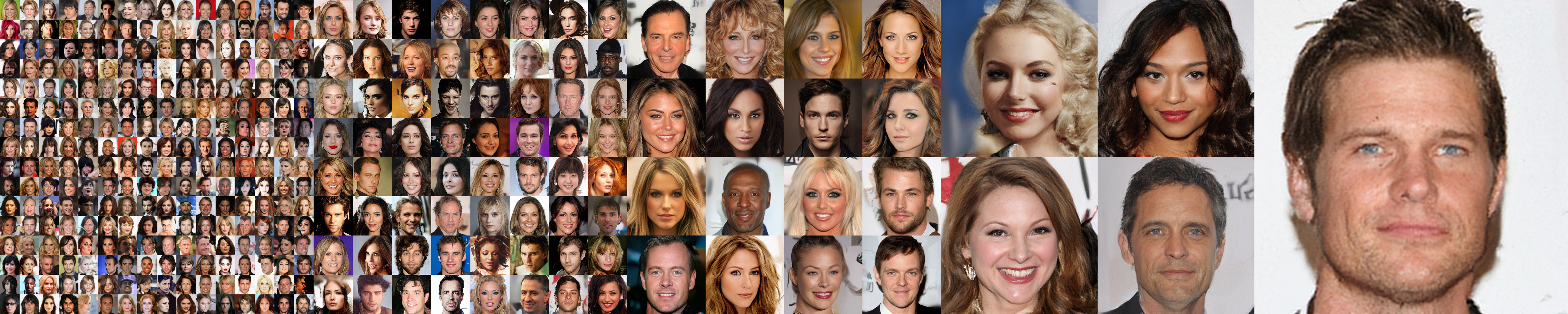
Figure 2: Modelling data as functions allows sampling at arbitrary resolutions using the same model with different sized noise. Left to right: $64\!\times\!64$, $128\!\times\!128$, $256\!\times\!256$ (original), $512\!\times\!512$, $1024\!\times\!1024$.

2 Background

Diffusion Models [Sohl-Dickstein et al., 2015, Ho et al., 2020] are probabilistic generative models that model the data distribution by learning to denoise data samples corrupted with noise. There are two main interpretations, discrete time and continuous time.

2.1 Discrete Time Diffusion

The discrete time interpretation is formed by defining a forward process $q(\boldsymbol{x}_{1:T}|\boldsymbol{x}_{0})$ that gradually adds noise to the data, $\boldsymbol{x}_{0}\sim q(\boldsymbol{x}_{0})$, over $T$ steps, resulting in a sequence of latent variables $\boldsymbol{x}_{1},\dots,\boldsymbol{x}_{T}$ such that $q(\boldsymbol{x}_{T})\approx\mathcal{N}(\boldsymbol{x}_{T};\boldsymbol{0},\boldsymbol{I})$. The reverse of this process can also be expressed as a Markov chain $p(\boldsymbol{x}_{0:T})$. Choosing Gaussian transition densities chosen to ensure these properties hold, the densities may be expressed as

$$q(\boldsymbol{x}_{1:T}|\boldsymbol{x}_{0})=\prod_{t=1}^{T}q(\boldsymbol{x}_{t}|\boldsymbol{x}_{t-1}),\qquad q(\boldsymbol{x}_{t}|\boldsymbol{x}_{t-1})=\mathcal{N}(\boldsymbol{x}_{t};\sqrt{1-\beta_{t}}\boldsymbol{x}_{t-1},\beta_{t}\boldsymbol{I}),$$ (1)

$$p(\boldsymbol{x}_{0:T})=p(\boldsymbol{x}_{T})\prod_{t=1}^{T}p(\boldsymbol{x}_{t-1}|\boldsymbol{x}_{t}),\qquad p(\boldsymbol{x}_{t-1}|\boldsymbol{x}_{t})=\mathcal{N}(\boldsymbol{x}_{t-1};\boldsymbol{\mu}_{\theta}(\boldsymbol{x}_{t},t),\boldsymbol{\Sigma}_{\theta}(\boldsymbol{x}_{t},t)),$$ (2)

where $0<\beta_{1},\dots,\beta_{T}<1$ is a pre-defined variance schedule and the covariance is typically of the form $\boldsymbol{\Sigma}_{\theta}(\boldsymbol{x}_{t},t)=\sigma_{t}^{2}\boldsymbol{I}$. Aiding training efficiency, $q(\boldsymbol{x}_{t}|\boldsymbol{x}_{0})$ can be expressed in closed form as $q(\boldsymbol{x}_{t}|\boldsymbol{x}_{0})=\mathcal{N}(\boldsymbol{x}_{t};\sqrt{\bar{\alpha}_{t}}\boldsymbol{x}_{0},(1-\bar{\alpha}_{t})\boldsymbol{I})$ where $\bar{\alpha}_{t}=\prod_{s=1}^{t}\alpha_{s}$ for $\alpha_{s}=1-\beta_{s}$. Training is possible by optimising the evidence lower bound on the negative log-likelihood which can be expressed as the KL-divergence between the forward process posteriors and backward transitions at each step

$$\mathcal{L}=\sum_{t\geq 1}\operatorname{\mathbb{E}}_{q}\left[D_{\text{KL}}(q(\boldsymbol{x}_{t-1}|\boldsymbol{x}_{t},\boldsymbol{x}_{0})\!\parallel\!p(\boldsymbol{x}_{t-1}|\boldsymbol{x}_{t}))\right]=\sum_{t\geq 1}\operatorname{\mathbb{E}}_{q}\left[\frac{1}{2\sigma_{t}^{2}}\|\tilde{\boldsymbol{\mu}}_{t}(\boldsymbol{x}_{t},\boldsymbol{x}_{0})-\boldsymbol{\mu}_{\theta}(\boldsymbol{x}_{t},t)\|_{2}^{2}\right]\!.$$ (3)

for $q(\boldsymbol{x}_{t-1}|\boldsymbol{x}_{t},\boldsymbol{x}_{0})=\mathcal{N}(\boldsymbol{x}_{t-1};\tilde{\boldsymbol{\mu}}_{t}(\boldsymbol{x}_{t},\boldsymbol{x}_{0}),\tilde{\beta}_{t}\boldsymbol{I})$, where $\tilde{\boldsymbol{\mu}}_{t}$ and $\tilde{\beta}_{t}$ can be derived in closed form. The connection between diffusion probabilistic models such as these, and denoising score-matching models can be made more explicit by making the approximation [De Bortoli et al., 2021],

$$p(\boldsymbol{x}_{t-1}|\boldsymbol{x}_{t}) =p(\boldsymbol{x}_{t}|\boldsymbol{x}_{t-1})\exp(\log p(\boldsymbol{x}_{t-1})-\log p(\boldsymbol{x}_{t}))$$ (4)

$$\approx\mathcal{N}(\boldsymbol{x}_{t-1};\sqrt{1-\beta_{t}}\boldsymbol{x}_{t}+\beta_{t}\nabla_{\boldsymbol{x}_{t}}\log p(\boldsymbol{x}_{t}),\beta_{t}\boldsymbol{I}),$$ (5)

which holds for small values of $\beta_{t}$. While $\nabla_{\boldsymbol{x}_{t}}\log p(\boldsymbol{x}_{t})$ is not available, it can be approximated using denoising score matching methods [Hyvärinen, 2005, Vincent, 2011]. Given that $\nabla_{\boldsymbol{x}_{t}}\log p(\boldsymbol{x}_{t})=\operatorname{\mathbb{E}}_{p(\boldsymbol{x}_{0}|\boldsymbol{x}_{t})}[\nabla_{\boldsymbol{x}_{t}}\log p(\boldsymbol{x}_{t}|\boldsymbol{x}_{0})]$ we can learn an approximation to the score with a neural network parameterised by $\theta$, $s_{\theta}(\boldsymbol{x}_{t},t)\approx\nabla\log p(\boldsymbol{x}_{t})$ [Song and Ermon, 2019], by minimising a reweighted variant of the ELBO (Eq. 3).

2.2 Continuous Time Diffusion

Song et al. [2021b] generalised the discrete time diffusion to an infinite number of noise scales, resulting in a stochastic differential equation (SDE) with trajectory $\{\boldsymbol{x}(t)\}_{t=0}^{T}$. The Markov chain defined in Eq. 1 is equivalent to an Euler-Maruyama discretisation of the following SDE

$$\mathop{}\!\mathrm{d}\boldsymbol{x}=f(\boldsymbol{x},t)\mathop{}\!\mathrm{d}t+g(t)\mathop{}\!\mathrm{d}\boldsymbol{w},\quad\boldsymbol{x}(0)\sim p_{0},\quad\boldsymbol{x}(T)\sim p_{T}.$$ (6)

where $\boldsymbol{w}$ is the standard Wiener process (Brownian motion), $f$ is the drift coefficient of the SDE, and $g$ is the diffusion coefficient. To allow inference, this SDE can be reversed; this can be written in the form of another SDE [Anderson, 1982]

$$\mathop{}\!\mathrm{d}\boldsymbol{x}=[f(\boldsymbol{x},t)-g(t)^{2}\nabla_{\boldsymbol{x}}\log p_{t}(\boldsymbol{x})]\mathop{}\!\mathrm{d}t+g(t)\mathop{}\!\mathrm{d}\bar{\boldsymbol{w}}.$$ (7)

where $\bar{\boldsymbol{w}}$ is the Wiener process in which time flows backward. The Markov chain defined in Eq. 5 is equivalent to an Euler-Maruyama discretisation of this SDE where the score function $\nabla_{\boldsymbol{x}}\log p_{t}(\boldsymbol{x})$ is approximated by $s_{\theta}(\boldsymbol{x},t)$. For all diffusion processes, there is an ordinary differential equation whose trajectories share the same distributions $\{p_{t}(\boldsymbol{x})\}_{t=1}^{T}$ as the SDE. The corresponding deterministic process for the SDE defined in Eq. 7 can be written as,

$$\mathop{}\!\mathrm{d}\boldsymbol{x}=\left[f(\boldsymbol{x},t)-\frac{1}{2}g(t)^{2}\nabla_{\boldsymbol{x}}\log p_{t}(\boldsymbol{x})\right]\mathop{}\!\mathrm{d}t,$$ (8)

referred to as the probability flow [Song et al., 2021b]. This deterministic interpretation has a number advantages such as faster sampling, and allowing exact-likelihoods to be calculated through the instantaneous change of variables formula [Chen et al., 2018].

3 Infinite Dimensional Diffusion Models

In contrast to previous generative diffusion models which assume that the data lies on a uniform grid, we assume that the data is a continuous function. For an introduction to infinite dimensional analysis see Da Prato [2006]. In this case, data points $x\sim q$ are functions defined on a separable Hilbert space $\mathcal{H}$ with domains $\mathbb{R}^{d}$ which are sampled from a probability distribution defined in the dual space of $\mathcal{H}$, $q\in\mathcal{H}^{*}$, i.e. $q:\mathcal{H}\to\mathbb{R}$; for simplicity we consider the case where $\mathcal{H}$ is the space of $L^{2}$ functions from $[0,1]^{n}$ to $\mathbb{R}^{d}$ although the following sections can be applied to other spaces. In this section we introduce infinite dimensional diffusion models which gradually destroy continuous signals until virtually no information remains.

3.1 White Noise Diffusion

One consideration to extend diffusion models to infinite dimensions is to use continuous white noise where each coordinate is an independent and identically distributed Gaussian random variable. In other words $\mathcal{N}(0,C_{I})$ where the covariance operator is $C_{I}(z(s),z(s^{\prime}))=\delta(s-s^{\prime})$, using the Dirac delta function $\delta$. The transition densities defined in Section 2.1 can be extended to infinite dimensions,

$$q(x_{t}|x_{t-1})=\mathcal{N}(x_{t};\sqrt{1-\beta_{t}}x_{t-1},\beta_{t}C_{I}),\quad p(x_{t-1}|x_{t})=\mathcal{N}(x_{t-1};\mu_{\theta}(x_{t},t),\Sigma_{\theta}(x_{t},t)),$$ (9)

where similar to the finite dimensional case we fix to $\Sigma_{\theta}(x_{t},t)=\sigma_{t}^{2}C_{I}$. While most similar to the finite dimensional approach, this method is problematic since white noise defined as such does not lie in $\mathcal{H}$ [Da Prato and Zabczyk, 2014] and therefore neither does $x_{t}$. However, in practice we are computationally unable to operate in infinite dimensions, instead we operate on a discretisation of the continuous space through an orthogonal projection, in which case the norm is finite. That is, if each $x$ has $n$ spatial dimensions, then the coordinate space is $D=[0,1]^{n}$; by sampling $m$ coordinates, $\boldsymbol{c}\in\left(\!\begin{smallmatrix}D\\ m\end{smallmatrix}\!\right)$ we thereby discretise $x$ as $x(\boldsymbol{c})\in\mathbb{R}^{m\times d}$. We can therefore approximate Eq. 3 by Monte-Carlo approximating each function, where we assume that $\tilde{\mu}$ and $\mu_{\theta}$ are able to operate on subsets through calculation in closed form or approximation,

$$\mathcal{L}=\sum_{t=1}^{T}\operatorname{\mathbb{E}}_{q(x_{t})}\operatorname{\mathbb{E}}_{\boldsymbol{c}\sim U\left(\left(\!\begin{smallmatrix}D\\ m\end{smallmatrix}\!\right)\right)}\left[\|\tilde{\mu}(x_{t}(\boldsymbol{c}),x_{0}(\boldsymbol{c}))-\mu_{\theta}(x_{t}(\boldsymbol{c}),t)\|_{2}^{2}\right].$$ (10)

Figure 3: Example Diffusion Processes. Mollified diffusion smooths diffusion states allowing the space to be more effectively modelled with continuous operators.

3.2 Smoothing States with Mollified Diffusion

While we can can build a generative model with white noise, in practice we may be using a neural architecture which assumes the input does lie in $\mathcal{H}$. Because of this, we propose an alternative diffusion process that approximates the non-smooth input space with a smooth function by convolving functions with a mollifier $T$ e.g. a trunctated Gaussian kernel. Convolving white noise in such a manner results in a Gaussian random field [Higdon, 2002]. Using the property that a linear transformation $y=Tx+b$ of a normally distributed variable $x\sim\mathcal{N}(\mu,C)$ is given by $y\sim\mathcal{N}(T\mu+b,TCT^{t})$, where ^t is the transpose operator, mollifying $q(x_{t}|x_{0})$ results in,

$$q(x_{t}|x_{0}) =\mathcal{N}(x_{t};\sqrt{\bar{\alpha}_{t}}Tx_{0},(1-\bar{\alpha}_{t})TT^{t}).$$ (11)

From this we are able to derive a closed form representation of the posterior (proof in Section B.1),

$$\begin{gathered}q(x_{t-1}|x_{t},x_{0})=\mathcal{N}(x_{t-1}|\tilde{\mu}_{t}(x_{t},x_{0}),\tilde{\beta}_{t}TT^{t}),\\ \text{where}\quad\tilde{\mu}_{t}(x_{t},x_{0})=\frac{\sqrt{\bar{\alpha}_{t-1}}\beta_{t}}{1-\bar{\alpha}_{t}}Tx_{0}+\frac{\sqrt{\alpha_{t}}(1-\bar{\alpha}_{t-1})}{1-\bar{\alpha}_{t}}x_{t}\quad\text{and}\quad\tilde{\beta}_{t}=\frac{1-\bar{\alpha}_{t-1}}{1-\bar{\alpha}_{t}}\beta_{t}.\end{gathered}$$ (12)

Defining the reverse transitions similarly as mollified Gaussian densities, $p_{\theta}(x_{t-1}|x_{t})=\mathcal{N}(x_{t-1}|\mu_{\theta}(x_{t},t),\sigma_{t}^{2}TT^{t})$, then we can parameterise $\mu_{\theta}:\mathcal{H}\to\mathcal{H}$ to directly predict $x_{0}$. The loss defined in Eq. 3 can be extended to infinite dimensions [Pinski et al., 2015], which in contrast to the approach in Section 3.1 is well defined in infinite dimensions (see Section B.2). However, a key finding of Ho et al. [2020] is that reparameterising to predict the noise yields much higher image quality. In this case, directly predicting white noise is impractical due to the continuous nature of $\mu_{\theta}$. Instead, we reparameterise $\mu_{\theta}$ to predict $T\xi$, for $\xi\sim\mathcal{N}(0,C_{I})$, motivated by the rewriting the loss as

$$\mathcal{L}_{t-1}=\operatorname{\mathbb{E}}_{q}\left[\frac{1}{2\sigma_{t}^{2}}\left\|T^{-1}\left(\frac{1}{\sqrt{\alpha_{t}}}\left(x_{t}(x_{0},\xi)-\frac{\beta_{t}}{\sqrt{1-\bar{\alpha_{t}}}}T\xi\right)-\mu_{\theta}(x_{t},t)\right)\right\|_{\mathcal{H}}^{2}\right],$$ (13)

$$\mu_{\theta}(x_{t},t)=\frac{1}{\sqrt{\alpha_{t}}}\left[x_{t}-\frac{\beta_{t}}{\sqrt{1-\bar{\alpha}_{t}}}f_{\theta}(x_{t},t)\right].$$ (14)

Directly predicting $x_{0}$ inherently gives an estimate of the unmollified data, but when predicting $T\xi$ we are only able to sample $Tx_{0}$, however, we can undo this process using a Wiener filter. While a similar technique could be used to calculate the loss, in this case $T^{-1}$ does not affect the minima so we can instead use $\mathcal{L}^{\text{simple}}_{t-1}=\operatorname{\mathbb{E}}_{q}[\left\|f_{\theta}(x_{t},t)-T\xi\right\|^{2}_{\mathcal{H}}]$. It is also possible to define a diffusion process where only the noise is mollified, however, we found this to not work well likely because the noise becomes of lower frequency than the underlying data. We can also directly apply the DDIM variation of DDPMs [Song et al., 2021a] to this setting, resulting in a deterministic sampling process from $T\xi$.

3.3 Continuous Time Diffusion

To examine the properties of the proposed infinite dimensional diffusion process, we consider infinite dimensional stochastic differential equations, which have been well studied. Specifically, SDEs taking values in a Banach space $\mathcal{X}$ continuously embedded into a separable Hilbert space $\mathcal{H}$,

$$\mathop{}\!\mathrm{d}x=F(x,t)\mathop{}\!\mathrm{d}t+\sqrt{2}\mathop{}\!\mathrm{d}w(t),$$ (15)

where the drift $F$ takes values in $\mathcal{H}$, the process $x$ takes values in $\mathcal{X}$, and $w$ is a cylindrical Wiener process on $\mathcal{H}$, a natural generalisation of finite dimensional Brownian motion. Infinite-dimensional SDEs have a unique strong solution as long as the coefficients satisfy some regularity conditions [Gawarecki and Mandrekar, 2010], in particular, the Lipschitz condition is met if for all $x,y\in C([0,T],\mathcal{H})$, $0\leq t\leq T$, there exists $h>0$ such that

$$\|F(x,t)-F(y,t)\|_{\mathcal{H}}\leq h\sup_{0\leq s\leq T}\|x(s)-y(s)\|.$$ (16)

Similar to the finite-dimensional case, the reverse time diffusion can be described by another SDE that runs backwards in time [Föllmer and Wakolbinger, 1986],

$$\mathop{}\!\mathrm{d}x=[F(x,t)-2D\log p_{t}(x)]\mathop{}\!\mathrm{d}t+\sqrt{2}\mathop{}\!\mathrm{d}\bar{w}(t).$$ (17)

However, unlike the finite-dimensional case, this only holds under certain conditions. If the interaction is too strong then the terminal position of the SDE may contain so much information that it is possible to reconstruct the trajectory of any coordinate. This is avoided by ensuring the drift terms have finite energy, $\operatorname{\mathbb{E}}[\int_{0}^{T}F^{i}(x,t)^{2}\mathop{}\!\mathrm{d}t]<\infty$, $\forall i\in D$. Mollifying the diffusion space is similar to preconditioning SDEs; MCMC approaches obtained by discretising such SDEs yeild compelling properties such as sampling speeds robust under mesh refinement [Cotter et al., 2013].

4 Parameterising the Diffusion Process

In order to model the score-function in Hilbert space, there are certain properties that is essential for the class of learnable functions to satisfy so as to allow training on infinite resolution data:

1. Can take as input points positioned at arbitrary coordinates.

2. Generalises to different numbers of input points than trained on, sampled on a regular grid.

3. Able to capture both global and local information.

4. Scales to very large numbers of input points, i.e. efficient in terms of runtime and memory.

Recent diffusion models often use a U-Net [Ronneberger et al., 2015] consisting of a convolutional encoder and decoder with skip-connections between resolutions allowing both global and local information to be efficiently captured. Unfortunately, U-Nets function on a fixed grid making them unsuitable. However, we can take inspiration to build an architecture satisfying the desired properties.

4.1 Neural Operators

Neural Operators [Li et al., 2020, Kovachki et al., 2021] are a framework designed for efficiently solving partial differential equations by learning to directly map the PDE parameters to the solution in a single step. However, more generally they are able to learn a map between two infinite dimensional function spaces making them suitable for parameterising an infinite dimensional diffusion model.

Let $\mathcal{X}$ and $\mathcal{S}$ be separable Banach spaces representing the spaces of noisy denoised data respectfully; a neural operator is a map $\mathcal{F}_{\theta}\colon\mathcal{X}\to\mathcal{S}$. Since $x\in\mathcal{X}$ and $s\in\mathcal{S}$ are both functions, we only have access to pointwise evaluations. Let $\boldsymbol{c}\in\left(\!\begin{smallmatrix}D\\ m\end{smallmatrix}\!\right)$ be an $m$-point discretisation of the domain and assume we have observations $x(\boldsymbol{c})\in\operatorname{\mathbb{R}}^{m\times d}$. To be discretisation invariant, the neural operator may be evaluated at any $c\in D$, potentially $c\notin\boldsymbol{c}$, thereby allowing a transfer of solutions between different discretisations i.e. satisfying properties 1 and 2. Each operator layer is built using a non-local integral kernel operator, $\mathcal{K}(x;\phi)$, which aggregates information spatially,

$$(\mathcal{K}(x;\phi)v_{l})(c)=\int_{D}\kappa(c,b,x(c),x(b);\phi)v_{l}(b)\mathop{}\!\mathrm{d}b,\qquad\forall c\in D.$$ (18)

Deep networks can be built in a similar manner to conventional methods, by stacking layers of linear operators with non-linear activation functions, $v_{0}\mapsto v_{1}\mapsto\dots\mapsto v_{L}$ where $v_{l}\mapsto v_{l+1}$ is defined as

$$v_{l+1}(c)=\sigma(Wv_{l}(c)+(\mathcal{K}(x;\phi)v_{l})(c)),\qquad\forall c\in D,$$ (19)

for pointwise linear transformation $W\colon\operatorname{\mathbb{R}}^{d}\to\operatorname{\mathbb{R}}^{d}$ and non-linear activation function $\sigma\colon\operatorname{\mathbb{R}}\to\operatorname{\mathbb{R}}$.

Figure 4: $\infty$-Diff uses a hierarchical architecture that operates on irregularly sampled functions at the top level to efficiently capture fine details, and on fixed grids at the other levels to capture global structure. This approach allows scaling to complex high resolution data.

4.2 Architecture

While neural operators which satisfy all the required properties exist, such as Galerkin attention [Cao, 2021] (a softmax-free linear attention operator) and MLP-Mixers [Tolstikhin et al., 2021], scaling beyond small numbers of coordinates is still challenging due to the high memory costs associated with caching activations for backpropagation. Instead we design a U-Net inspired multiscale architecture (Fig. 4) that aggregates information locally and globally at different points through the network.

In a continuous setting, there are two main approaches to downsampling: (1) selecting a subset of coordinates [Wang and Golland, 2022] and (2) interpolating points to a regularly spaced grid [Rahman et al., 2022]. We found that with repeated application of (1), approximating integral operators on non-uniformly spaced grids with very few points did not perform nor generalise well, likely due to the high variance. On the other hand, while working with a regular grid removes some sparsity properties, issues with variance are much lower. As such, we use a hybrid approach with sparse operators applied on the raw data, which is then interpolated to a fixed grid and a grid-based architecture is applied; if the fixed grid is of sufficiently high dimension, this combination should be sufficient. While an FNO [Li et al., 2021, Rahman et al., 2022] architecture could be used, we achieved better results with dense convolutions [Nichol and Dhariwal, 2021], with sparse operators used for resolution changes.

At the sparse level we use convolution operators [Kovachki et al., 2021], finding them to be more performant than Galerkin attention, with global context no longer essential due to the multiscale architecture. In this case, the operator is defined using a translation invariant kernel restricted to the local neighbourhood of each coordinate, $N(c)$,

$$x(c)=\int_{\text{N}(c)}\kappa(c-y)v(y)\mathop{}\!\mathrm{d}y,\qquad\forall c\in D.$$ (20)

We restrict $\kappa$ to be a depthwise kernel due to the greater parameter efficiency for large kernels (particularly for continuously parameterised kernels) and finding that they are more able to generalise when trained with fewer sampled coordinates; although the sparsity ratio is the same for regular and depthwise convolutions, because there are substantially more values in a regular kernel, there is more spatial correlation between values. When a very large number of sampled coordinates are used, fully continuous convolutions are extremely impractical in terms of memory usage and run-time. In practice, however, images are obtained and stored on a discrete grid. As such, by treating images as high dimensional, but discrete entities, we can take advantage of efficient sparse convolution libraries [Choy et al., 2019, Contributors, 2022], making memory usage and run-times much more reasonable. Specifically, we use TorchSparse [Tang et al., 2022], modified to allow depthwise convolutions. Wang and Golland [2022] proposed using low discrepancy coordinate sequences to approximate the integrals due to their better convergence rates. However, we found uniformly sampled points to be more effective, likely because the reduced structure results in points sampled close together which allows high frequency details to be captured more easily.

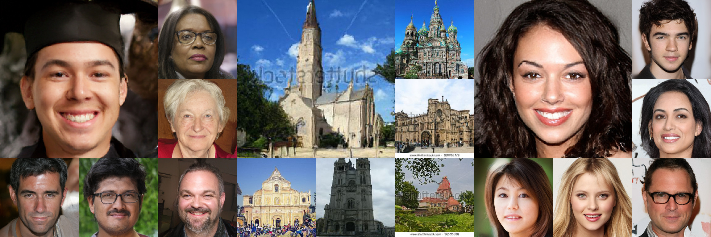
Figure 5: Samples from $\infty$-Diff models trained on sets of randomly subsampled coordinates.

Method	CelebAHQ-64	CelebAHQ-128	FFHQ-256	Church-256
Finite-Dimensional
CIPS [Anokhin et al., 2021]	-	-	5.29	10.80
StyleSwin [Zhang et al., 2022]	-	3.39	3.25	8.28
UT [Bond-Taylor et al., 2022]	-	-	3.05	5.52
StyleGAN2 [Karras et al., 2020]	-	2.20	2.35	6.21
Infinite-Dimensional
D2F [Dupont et al., 2022a]	40.4∗	-	-	-
DPF [Zhuang et al., 2023]	13.21∗	-	-	-
GEM [Du et al., 2021]	14.65	23.73	35.62	87.57
GASP [Dupont et al., 2022b]	9.29	27.31	24.37	37.46
$\boldsymbol{\infty}$-Diff (Ours)	4.57	3.02	3.87	10.36

Table 1: $\text{FID}_{\text{CLIP}}$ [Kynkäänniemi et al., 2023] evaluation against finite-dimensional methods as well as other infinite-dimensional approaches which are trained on coordinate subsets. ^∗=Inception FID.

5 Experiments

In this section we demonstrate that the proposed mollified diffusion process modelled with neural operator based networks and trained on coordinate subsets are able to generate high quality, high resolution samples. We explore the properties of this approach including discretisation invariance, the impact of the number of coordinates during training, and compare the sample quality of our approach with other infinite dimensional generative models. We train models on three $256\!\times\!256$ datasets, CelebA-HQ [Karras et al., 2018], FFHQ [Karras et al., 2019], and LSUN Church [Yu et al., 2015]; unless otherwise specified models are trained on $\nicefrac{{1}}{{4}}$ of pixels, randomly selected.

When training diffusion models, very large batch sizes are necessary due the high variance [Hoogeboom et al., 2023], making training on high resolution data on a single GPU impractical. To address this, we use the diffusion autoencoder framework [Preechakul et al., 2022] which reduces stochasticity by dividing the generation process into two stages. To encode data we use the first half of our proposed architecture (Fig. 4), which still operates on sparsely sampled coordinates. When sampling, we use the deterministic DDIM interpretation with 100 steps. Additional details are in Appendix A. Source code is available at https://github.com/samb-t/infty-diff.

Sample Quality

Samples from our approach can be found in Fig. 5 which are high quality, diverse, and capture fine details. In Table 1 we quantitatively compare with other approaches that treat inputs as infinite dimensional data, as well as more traditional approaches that assume data lies on a fixed grid. As proposed by Kynkäänniemi et al. [2023], we calculate FID [Heusel et al., 2017] using CLIP features [Radford et al., 2021] which is better correlated with human perception of image quality. Our approach scales to high resolutions much more effectively than the other function-based approaches as evidenced by the substantially lower scores. Visual comparison between samples from our approach and other function-based approaches can be found in Fig. 6 where samples from our approach can be seen to be higher quality and display more details without blurring or adversarial artefacts. All of these approaches are based on neural fields [Xie et al., 2022] where coordinates are treated independently; in contrast, our approach uses neural operators to transform functions using spatial context thereby allowing more details to be captured. Both GASP [Dupont et al., 2022b] and GEM [Du et al., 2021] rely on compressed latent-conditional hypernetworks which makes efficiently scaling difficult. D2F [Dupont et al., 2022a] relies on a deterministic compression stage which loses detail due to the finite vector size. DPF [Zhuang et al., 2023] uses small fixed sized coordinate subsets as global context with other coordinates modelled implicitly, thereby causing blur.

Discretisation Invariance

In Fig. 2 we demonstrate the discretisation invariance properties of our approach. After training on random coordinate subsets from $256\!\times\!256$ images, we can sample from this model at arbitrary resolutions which we show at resolutions from $64\!\times\!64$ to $1024\!\times\!1024$ by initialising the diffusion with different sized noise. We experimented with (alias-free) continuously parameterised kernels [Romero et al., 2022] but found bi-linearly interpolating kernels to be more effective. At each resolution, even exceeding the training data, samples are consistent and diverse. In Fig. 7 we analyse how the number of sampling steps affects quality at different sampling resolutions.

Coordinate Sparsity

One factor influencing the quality of samples is the number of coordinates sampled during training; fewer coordinates means fewer points from which to approximate each integral. We analyse the impact of this in Table 3, finding that as expected, performance decreases with fewer coordinates, however, this effect is fairly minimal. With fewer coordinates also comes substantial speedup and memory savings; at $256\!\times\!256$ with $\nicefrac{{1}}{{4}}$ coordinates the speedup is $1.4\times$.

Architecture Analysis

In Table 2 we ablate the impact of various architecture choices against the architecture described in Section 4.2, matching the architecture as closely as possible. In particular, sparse downsampling (performed by randomly subsampling coordinates; we observed similar with equidistant subsampling, Qi et al., 2017) fails to capture the distribution. Similarly using a spatially nonlinear kernel (Eq. 18), implemented as conv, activation, conv, does not generalise well unlike linear kernels (we observed similar for softmax transformers, Kovachki et al., 2021).

Figure 6: Qualitative comparison with other infinite dimensional approaches.

Figure 7: $\text{FID}_{\text{CLIP}}$ at various steps & resolutions.

Architecture	$\text{FID}_{\text{CLIP}}$
Sparse Downsample	85.99
Nonlinear Kernel	24.49
Quasi Monte Carlo	7.63
Regular Convs	5.63
$\boldsymbol{\infty}$-Diff (Ours)	4.75

Table 2: Architectural component ablations in terms of $\text{FID}_{\text{CLIP}}$.

Ratio	$\text{FID}_{\text{CLIP}}$	Speedup
1	3.15	$1.0\times$
$\nicefrac{{1}}{{2}}$	4.12	$1.0\times$
$\nicefrac{{1}}{{4}}$	4.75	$1.3\times$
$\nicefrac{{1}}{{8}}$	6.48	$1.6\times$

Table 3: Impact of coordinate sparsity on quality for FFHQ 128. $\text{FID}_{\text{CLIP}}$ calculated with 10k samples.

Figure 8: Super-resolution

Super-resolution

The discretisation invariance properties of the proposed approach makes superresolution a natural application. We evaluate this in a simple way, passing a low resolution image through the encoder, then sampling at a higher resolution; see Fig. 8 where it is clear that more details have been added. A downside of this specific approach is that information is lost in the encoding process, however, this could potentially by improved by incorporating DDIM encodings [Song et al., 2021a].

Figure 9: Inpainting.

Inpainting

Inpainting is possible with mollified diffusion (Fig. 9), using reconstruction guidance [Ho et al., 2022b], $x_{t-1}\leftarrow x_{t-1}-\lambda\nabla_{x_{t}}\|m\odot(\tilde{\mu}_{0}(x_{t},t)-T\bar{x})\|_{2}^{2}$ for inpainting mask $m$, learned estimate of $Tx_{0}$, $\tilde{\mu}_{0}$, and image to be inpainted $\bar{x}$. The diffusion autoencoder framework gives an additional level of control when inpainting since the reverse diffusion process can be applied to encodings from a chosen time step $t_{s}$, allowing control over how different the inpainted region is from the original image.

6 Discussion

There are a number of interesting directions to improve our approach including more powerful and efficient neural operators, more efficient sparse methods (including better optimised sparse convolutions), and better integral approximation for instance by adaptively sampling coordinates. One interesting architecture direction is RIN [Jabri et al., 2022] which adaptively allocates compute to complex regions. Other approaches for high resolution diffusion models have focused on architectural improvements and noise schedules [Hoogeboom et al., 2023]. In contrast, we reduce runtime and memory usage through sparsity; many of these improvements are complementary to our approach.

In recent years there have been a number of advances in the study of diffusion models which are also complementary to our approach, these include consistency models [Song et al., 2023] which form single/few-step generative models from diffusion models, mapping between arbitrary densities [Albergo et al., 2023], and reducing sampling times via Schrödinger bridges [De Bortoli et al., 2021], critically-damped diffusion [Dockhorn et al., 2022], and faster solvers [Lu et al., 2022]. Similar to our proposal of mollifying the diffusion process, a number of recent works have used blurring operations to improve diffusion. Rissanen et al. [2023] corrupt data by repeatedly blurring images until they are approximately a single colour; due to the deterministic nature of this process, noise is added to split paths. This process is formalised further by Hoogeboom and Salimans [2023].

Concurrent with this work, a number of methods independently proposed approaches for modelling diffusion models in infinite dimensions [Lim et al., 2023, Franzese et al., 2023, Hagemann et al., 2023, Zhuang et al., 2023], these approaches are complementary to ours and distinct in a number of ways. In particular, none of these approaches offer the ability to scale to high resolution data demonstrated in this work, typically being only applied to very simple data (e.g. Gaussian mixtures and MNIST). These approaches all rely on either conditional neural fields or operating on uniform grids of coordinates, whereas our approach operates directly on raw sparse data, enabling better scaling. The closest to our work in terms of scalability is Diffusion Probabilistic Fields [Zhuang et al., 2023] which denoises each coordinate independently, using a small subset of coordinates to provide context, however, this is considerably more restrictive than our approach and computational inefficiency limits resolutions to be much smaller than ours (up to $64\!\times\!64$).

There are a number of other neural field GAN approaches similar to GASP [Dupont et al., 2022b] such as CIPS [Anokhin et al., 2021] and Poly-INR [Singh et al., 2023], however, these approaches rely on convolutional discriminators thereby requiring all coordinates from fixed size images, preventing scaling to effectively infinite resolutions. Also of relevance are Neural Processes [Garnelo et al., 2018, Dutordoir et al., 2022] which also learn distributions over functions similar to Gaussian Processes. However, these approaches address conditional inference, whereas we construct an unconditional generative model that is applied to substantially more complex data such as high resolution images.

7 Conclusion

In conclusion, we found that mollified-state diffusion models with transition densities represented by neural operators are able to generate high quality infinite dimensional samples. Despite only observing subsets of pixels during training, sample quality is competitive with state-of-the-art models trained on all pixels at once. Prior infinite dimensional approaches use latent conditional neural fields; our findings demonstrate that sparse neural operators which operate directly on raw data are a capable alternative, offering significant advantages by not treating all coordinates independently, as evidenced by substantially lower FID scores. Future work would benefit from improved neural operators that can effectively operate at greater levels of sparsity to further improve the efficiency of our approach.

Appendix A Implementation Details

All $256\!\times\!256$ models are trained on a single NVIDIA A100 80GB GPU using automatic mixed precision. Optimisation is performed using the Adam optimiser [Kingma and Ba, 2015] with a batch size of 32 and learning rate of $5\!\times\!10^{-5}$; each model being trained to optimise validation loss. Each model is trained as a diffusion autoencoder to reduce training variance, allowing much smaller batch sizes thereby permitting training on a single GPU. A latent size of 1024 is used and the latent model architecture and diffusion hyperparameters are the same as used by Preechakul et al. [2022]. In image space, the diffusion model uses a cosine noise schedule [Nichol and Dhariwal, 2021] with 1000 steps. Mollifying is performed with Gaussian blur with a variance of $1.0$.

For the image-space architecture, 3 sparse residual convolution operator blocks are used on the sparse data. Each of these consist of a single depthwise sparse convolution layer with kernel size 7 and 64 channels with the output normalised by the total number of coordinates in each local region, followed by a three layer MLP; modulated layer normalisation [Ba et al., 2016, Nichol and Dhariwal, 2021] is used to normalise and condition on the diffusion time step. These blocks use larger convolution kernels than typically used in diffusion model architectures to increase the number of coordinates present in the kernel when a small number of coordinates are sampled. Using large kernel sizes paired with MLPs has found success in recent classification models such as ConvNeXt [Liu et al., 2022].

As mentioned in Section 4.2, for the grid-based component of our architecture we experimented with a variety of U-Net shaped fourier neural operator [Li et al., 2021, Rahman et al., 2022] architectures; although these more naturally allow resolution changes at those levels, we found this came with a substantial drop in performance. This was even the case when operating at different resolutions. As such, we use the architecture used by Nichol and Dhariwal [2021] fixed at a resolution of $128\!\times\!128$; the highest resolution uses 128 channels which is doubled at each successive resolution up to a maximum factor of 8; attention is applied at resolutions 16 and 8, as is dropout, as suggested by Hoogeboom et al. [2023]. Although this places more emphasis on the sparse operators for changes in sampling resolution, we found this approach to yield better sample quality across the board.

A.1 Table 1 Experiment Details

In Table 1 we compare against a number of other approaches in terms of $\text{FID}_{\text{CLIP}}$. In each case scores are calculated by comparing samples against full datasets, with 30k samples used for CelebA-HQ and 50k samples used for FFHQ and LSUN Church. For the finite-dimensional approaches we use the official code and released models in all cases to generate samples for calculating $\text{FID}_{\text{CLIP}}$ scores. To provide additional context for CelebA-HQ $128\!\times\!128$ we provide scores for StyleGAN2 and StyleSwin where samples are downsampled from $256\!\times\!256$.

For GASP [Dupont et al., 2022b] we use the official code and pretrained models for CelebA-HQ at resolutions $64\!\times\!64$ and $128\!\times\!128$; for FFHQ and LSUN Church we train models using the same generator hyperparameters as used for all experiments in that work and for the discriminator we scale the model used for CelebA-HQ $128\!\times\!128$ by adding an additional block to account for the resolution change. These models were trained by randomly sampling $\nicefrac{{1}}{{4}}$ of coordinates at each training step to match what was used to train our models.

Similarly, for GEM [Du et al., 2021] we use the official code and train models on CelebA-HQ $128\!\times\!128$, FFHQ and LSUN Church, using the same hyperparameters as used for all experiments in that work (which are independent of modality/resolution); we implement sampling as described in Section 4.4 of that paper by randomly sampling a latent corresponding to a data point, linearly interpolating to a neighbouring latent and adding a small amount of Gaussian noise (chosen with standard deviation between 0 and 1 to optimise sample quality/diversity) and then projected onto the local manifold. Because GEM is based on the autodecoder framework where latents are allocated per datapoint and jointly optimised with the model parameters, training times are proportional to the number of points in the dataset. As such, the FID scores for LSUN Church in particular are especially poor due to the large scale of the dataset.

Appendix B Mollified Diffusion Derivation

In this section we derive the mollified diffusion process proposed in Section 3.2.

B.1 Forward Process

We start by specifically choosing $q(x_{0}|x_{t})$ as defined by Section 2.1 where states are mollified by $T$,

$$q(x_{t-1}|x_{0}) =\mathcal{N}(x_{t-1}|\sqrt{\bar{\alpha}_{t-1}}Tx_{0},(1-\bar{\alpha}_{t-1})TT^{t}),$$ (21)

$$q(x_{t}|x_{0}) =\mathcal{N}(x_{t}|\sqrt{\bar{\alpha}_{t}}Tx_{0},(1-\bar{\alpha}_{t})TT^{t}),$$ (22)

from which we wish to find the corresponding representation of $q(x_{t-1}|x_{t},x_{0})$. The solution to this is given by Bishop and Nasrabadi [2006, Equations 2.113 to 2.117], where we write

$$q(x_{t}|x_{0}) =\mathcal{N}(x_{t}|\mu,\Lambda^{-1}),$$ (23)

$$q(x_{t-1}|x_{0}) =\mathcal{N}(x_{t-1}|A\mu+b,L^{-1}+A\Lambda^{-1}A^{t}),$$ (24)

$$q(x_{t-1}|x_{t},x_{0}) =\mathcal{N}(x_{t-1}|Ax_{t}+b,L^{-1}).$$ (25)

From this we can immediately see that $\mu=\sqrt{\bar{\alpha}_{t}}Tx_{0}$ and $\Lambda^{-1}=(1-\bar{\alpha}_{t})TT^{t}$. Additionally, $A\mu+b=A\sqrt{\bar{\alpha}_{t}}Tx_{0}+b=\sqrt{\bar{\alpha}_{t-1}}Tx_{0}$, therefore we can modify the approach by Ho et al. [2020], including $T$ where relevant and set $A$, $b$ and $L^{-1}$ as

$$A =\frac{\sqrt{\alpha_{t}}(1-\bar{\alpha}_{t-1})}{1-\bar{\alpha}_{t}}I, b =\frac{\sqrt{\bar{\alpha}_{t-1}}\beta_{t}}{1-\bar{\alpha}_{t}}Tx_{0}, L^{-1} =\frac{1-\bar{\alpha}_{t-1}}{1-\bar{\alpha}_{t}}\beta_{t}TT^{t}$$ (26)

This can be shown to be correct by passing $A$, $b$, and $L^{-1}$ into equations Eqs. 23, 24 and 25, first:

$$A\mu+b =\frac{\sqrt{\bar{\alpha}_{t}}\sqrt{\alpha_{t}}(1-\bar{\alpha}_{t-1})}{1-\bar{\alpha}_{t}}Tx_{0}+b$$ (27)

$$=\frac{\sqrt{\bar{\alpha}_{t}}\sqrt{\alpha_{t}}(1-\bar{\alpha}_{t-1})+\sqrt{\bar{\alpha}_{t-1}}(1-\alpha_{t})}{1-\bar{\alpha}_{t}}Tx_{0}$$ (28)

$$=\frac{\sqrt{\bar{\alpha}_{t-1}}(\alpha_{t}-\bar{\alpha}_{t}+1-\alpha_{t})}{1-\bar{\alpha}_{t}}Tx_{0}=\sqrt{\bar{\alpha}_{t-1}}Tx_{0},$$ (29)

and secondly,

$$L^{-1}+A\Lambda^{-1}A^{T} =\frac{(1-\bar{\alpha}_{t-1})(1-\alpha_{t})}{1-\bar{\alpha}_{t}}TT^{t}+\frac{\alpha_{t}(1-\bar{\alpha}_{t-1})^{2}(1-\bar{\alpha}_{t})}{(1-\bar{\alpha}_{t})^{2}}TT^{t}$$ (30)

$$=\frac{1-\bar{\alpha}_{t-1}-\alpha_{t}+\bar{\alpha_{t}}+\alpha_{t}-2\bar{\alpha}_{t}+\alpha_{t}\bar{\alpha}_{t-1}^{2}}{1-\bar{\alpha}_{t}}=(1-\bar{\alpha}_{t-1})TT^{t}$$ (31)

$$=\frac{(1-\bar{\alpha}_{t})(1-\bar{\alpha}_{t-1})}{1-\bar{\alpha}_{t}}TT^{t}=(1-\bar{\alpha}_{t-1})TT^{t},$$ (32)

which together form $q(x_{t-1}|x_{0})$.

B.2 Reverse Process

In this section we derive the loss for optimising the proposed mollified diffusion process and discuss the options for parameterising the model. As stated in Section 3.2, we define the reverse transition densities as

$$p_{\theta}(x_{t-1}|x_{t})=\mathcal{N}(x_{t-1}|\mu_{\theta}(x_{t},t),\sigma_{t}^{2}TT^{t}),$$ (33)

where $\sigma_{t}^{2}=\beta_{t}$ or $\sigma_{t}^{2}=\tilde{\beta}_{t}$. From this we can calculate the loss at time $t-1$ in the same manner as the finite-dimensional case (Eq. 3) by calculating the Kullback-Leibler divergence in infinite dimensions [Pinski et al., 2015], for conciseness we ignore additive constants throughout since they do not affect optimisation,

$$\mathcal{L}_{t-1}=\mathbb{E}_{q}\left[\frac{1}{2\sigma_{t}^{2}}\bigg{\|}T^{-1}(\tilde{\mu}_{t}(x_{t},x_{0})-\mu_{\theta}(x_{t},t))\bigg{\|}_{\mathcal{H}}^{2}\right].$$ (34)

To find a good representation for $\mu_{\theta}$ we expand out $\tilde{\mu}_{t}$ as defined in Eq. 12 in the above loss giving

$$\mathcal{L}_{t-1}=\mathbb{E}_{q}\left[\frac{1}{2\sigma_{t}^{2}}\left\|T^{-1}\left(\frac{\sqrt{\bar{\alpha}_{t-1}}\beta_{t}}{1-\bar{\alpha}_{t}}Tx_{0}+\frac{\sqrt{\alpha_{t}}(1-\bar{\alpha}_{t-1})}{1-\bar{\alpha}_{t}}x_{t}-\mu_{\theta}(x_{t},t)\right)\right\|_{\mathcal{H}}^{2}\right].$$ (35)

From this we can see that one possible parameterisation is to directly predict $x_{0}$, that is,

$$\mu_{\theta}(x_{t},t)=\frac{\sqrt{\bar{\alpha}_{t-1}}\beta_{t}}{1-\bar{\alpha}_{t}}Tf_{\theta}(x_{t},t)+\frac{\sqrt{\alpha_{t}}(1-\bar{\alpha}_{t-1})}{1-\bar{\alpha}_{t}}x_{t}.$$ (36)

This parameterisation is interesting because when sampling, we can use the output of $f_{\theta}$ to directly obtain an estimate of the unmollified data. Additionally, when calculating the loss $\mathcal{L}_{t-1}$, all $T$ and $T^{-1}$ terms cancel out meaning there are no concerns with reversing the mollification during training, which can be numerically unstable. To see this, we can further expand out Eq. 35 using the parameterisation of $\mu_{\theta}$ defined in Eq. 36,

$$\begin{split}\mathcal{L}_{t-1}&=\mathbb{E}_{q}\Bigg{[}\frac{1}{2\sigma_{t}^{2}}\bigg{\|}T^{-1}\bigg{(}\frac{\sqrt{\bar{\alpha}_{t-1}}\beta_{t}}{1-\bar{\alpha}_{t}}Tx_{0}+\frac{\sqrt{\alpha_{t}}(1-\bar{\alpha}_{t-1})}{1-\bar{\alpha}_{t}}x_{t}\\ &\hskip 100.00015pt-\frac{\sqrt{\bar{\alpha}_{t-1}}\beta_{t}}{1-\bar{\alpha}_{t}}Tf_{\theta}(x_{t},t)-\frac{\sqrt{\alpha_{t}}(1-\bar{\alpha}_{t-1})}{1-\bar{\alpha}_{t}}x_{t}\bigg{)}\bigg{\|}_{\mathcal{H}}^{2}\Bigg{]}\end{split}$$ (37)

$$=\mathbb{E}_{q}\left[\frac{1}{2\sigma_{t}^{2}}\left\|\frac{\sqrt{\bar{\alpha}_{t-1}}\beta_{t}}{1-\bar{\alpha}_{t}}x_{0}-\frac{\sqrt{\bar{\alpha}_{t-1}}\beta_{t}}{1-\bar{\alpha}_{t}}f_{\theta}(x_{t},t)\right\|_{\mathcal{H}}^{2}\right]$$ (38)

$$=\mathbb{E}_{q}\left[\frac{\sqrt{\bar{\alpha}_{t-1}}\beta_{t}}{2\sigma_{t}^{2}(1-\bar{\alpha}_{t})}\left\|x_{0}-f_{\theta}(x_{t},t)\right\|_{\mathcal{H}}^{2}\right].$$ (39)

Using this parameterisation, we can sample from $p_{\theta}(x_{t-1}|x_{t})$ as

$$x_{t-1}=\frac{\sqrt{\alpha_{t}}(1-\bar{\alpha}_{t-1})}{1-\bar{\alpha}_{t}}x_{t}+T\left(\frac{\sqrt{\bar{\alpha}_{t-1}}\beta_{t}}{1-\bar{\alpha}_{t}}f_{\theta}(x_{t},t)+\sigma_{t}\xi\right)\quad\text{where}\quad\xi\sim\mathcal{N}(0,C_{I}).$$ (40)

Alternatively, we can parameterise $\tilde{\mu}$ to predict the noise $\xi$ rather than $x_{0}$, which was found by Ho et al. [2020] to yield higher sample quality. To see this, we can write Eq. 11 as $x_{t}(x_{0},\xi)=\sqrt{\bar{\alpha}_{t}}Tx_{0}+\sqrt{1-\bar{\alpha}_{t}}T\xi$. Expanding out Eq. 34 with this gives the following loss,

$$\mathcal{L}_{t-1} =\operatorname{\mathbb{E}}_{q}\left[\frac{1}{2\sigma_{t}^{2}}\bigg{\|}T^{-1}\bigg{(}\tilde{\mu}(x_{t},x_{0})-\mu_{\theta}(x_{t},t)\bigg{)}\bigg{\|}^{2}_{\mathcal{H}}\right]$$ (41)

$$=\operatorname{\mathbb{E}}_{q}\left[\frac{1}{2\sigma_{t}^{2}}\bigg{\|}T^{-1}\bigg{(}\tilde{\mu}(x_{t}(x_{0},\xi),\frac{1}{\sqrt{\bar{\alpha}_{t}}}T^{-1}(x_{t}(x_{0},\xi)-\sqrt{1-\bar{\alpha}_{t}}T\xi))-\mu_{\theta}(x_{t},t)\bigg{)}\bigg{\|}^{2}_{\mathcal{H}}\right]$$ (42)

$$=\operatorname{\mathbb{E}}_{q}\left[\frac{1}{2\sigma_{t}^{2}}\left\|T^{-1}\left(\frac{1}{\sqrt{\alpha_{t}}}\left(x_{t}(x_{0},\xi)-\frac{\beta_{t}}{\sqrt{1-\bar{\alpha_{t}}}}T\xi\right)-\mu_{\theta}(x_{t},t)\right)\right\|^{2}_{\mathcal{H}}\right].$$ (43)

Since directly predicting $\xi$ would require predicting a non-continuous function, we instead propose predicting $T\xi$ which is a continuous function, giving the following parameterisation and loss,

$$\mu_{\theta}(x_{t},t)=\frac{1}{\sqrt{\alpha_{t}}}\left[x_{t}-\frac{\beta_{t}}{\sqrt{1-\bar{\alpha}_{t}}}f_{\theta}(x_{t},t)\right],$$ (44)

$$\mathcal{L}_{t-1}=\operatorname{\mathbb{E}}_{q}\left[\frac{1}{2\sigma_{t}^{2}}\left\|\frac{1}{\sqrt{\alpha_{t}}}T^{-1}\left(\frac{\beta_{t}}{\sqrt{1-\bar{\alpha}_{t}}}f_{\theta}(x_{t},t)-\frac{\beta_{t}}{\sqrt{1-\bar{\alpha_{t}}}}T\xi\right)\right\|^{2}_{\mathcal{H}}\right].$$ (45)

In this case $T^{-1}$ is a linear transformation that does not affect the minima. In addition to this, we can remove the weights as suggested by Ho et al. [2020], giving the following proxy loss,

$$\mathcal{L}^{\text{simple}}_{t-1} =\operatorname{\mathbb{E}}_{q}\left[\left\|f_{\theta}(x_{t},t)-T\xi\right\|^{2}_{\mathcal{H}}\right].$$ (46)

An alternative parameterisation which can train more reliably is $v$-prediction [Salimans and Ho, 2022, Hoogeboom et al., 2023]; we experimented with this parameterisation but found mollified noise prediction to yield higher quality samples.

Appendix C Additional Results

In this section we provide additional samples from our models to visually assess quality. Detecting overfitting is crucial when training generative models. Scores such as FID are unable to detect overfitting, making identifying overfitting difficult in approaches such as GANs. Because diffusion models are trained to optimise a bound on the likelihood, training can be stopped to minimise validation loss. As further evidence we provide nearest neighbour images from the training data to samples from our model, measured using LPIPS [Zhang et al., 2018].

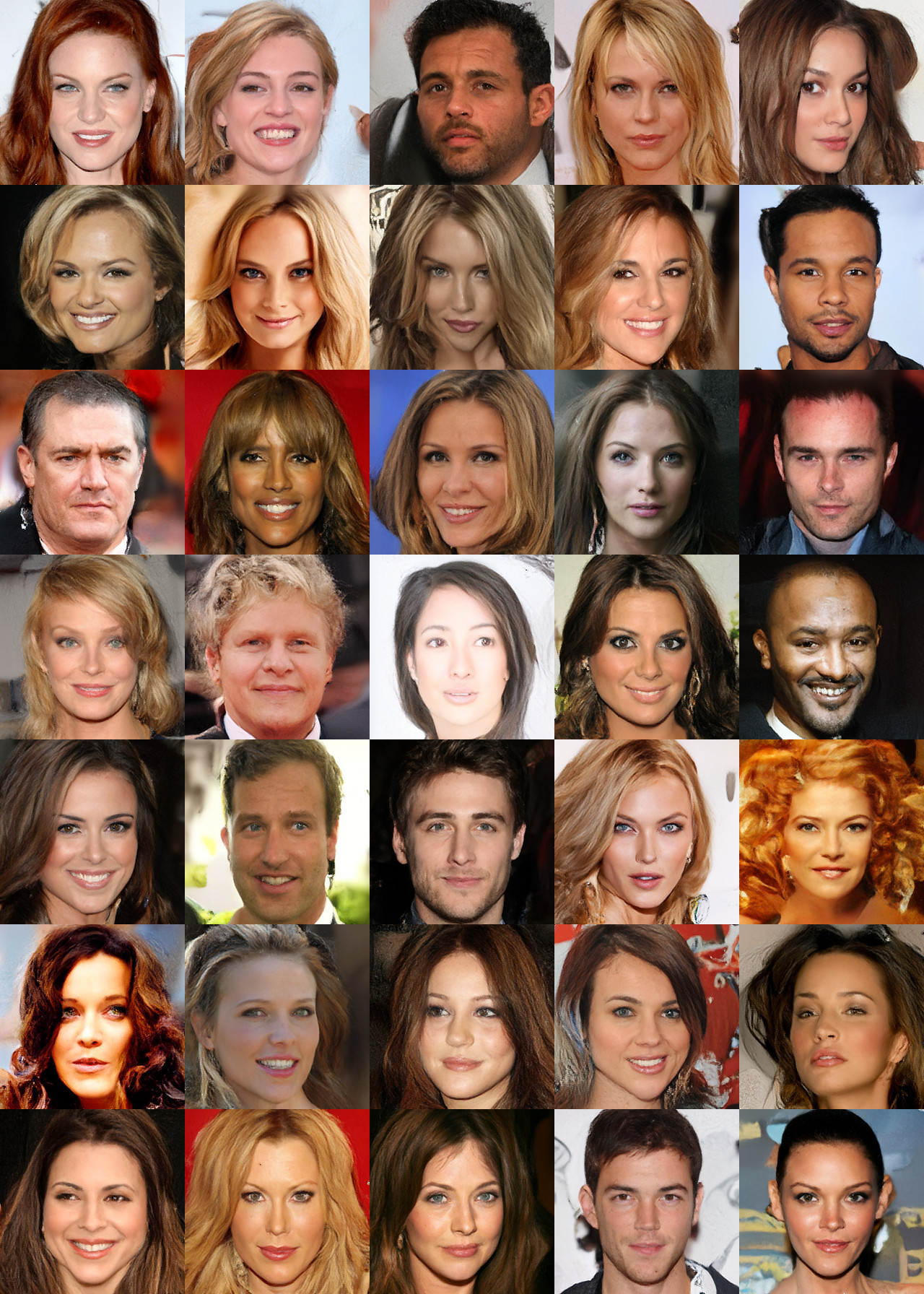
Figure 10: Non-cherry picked, CelebA-HQ $256\!\times\!256$ samples.

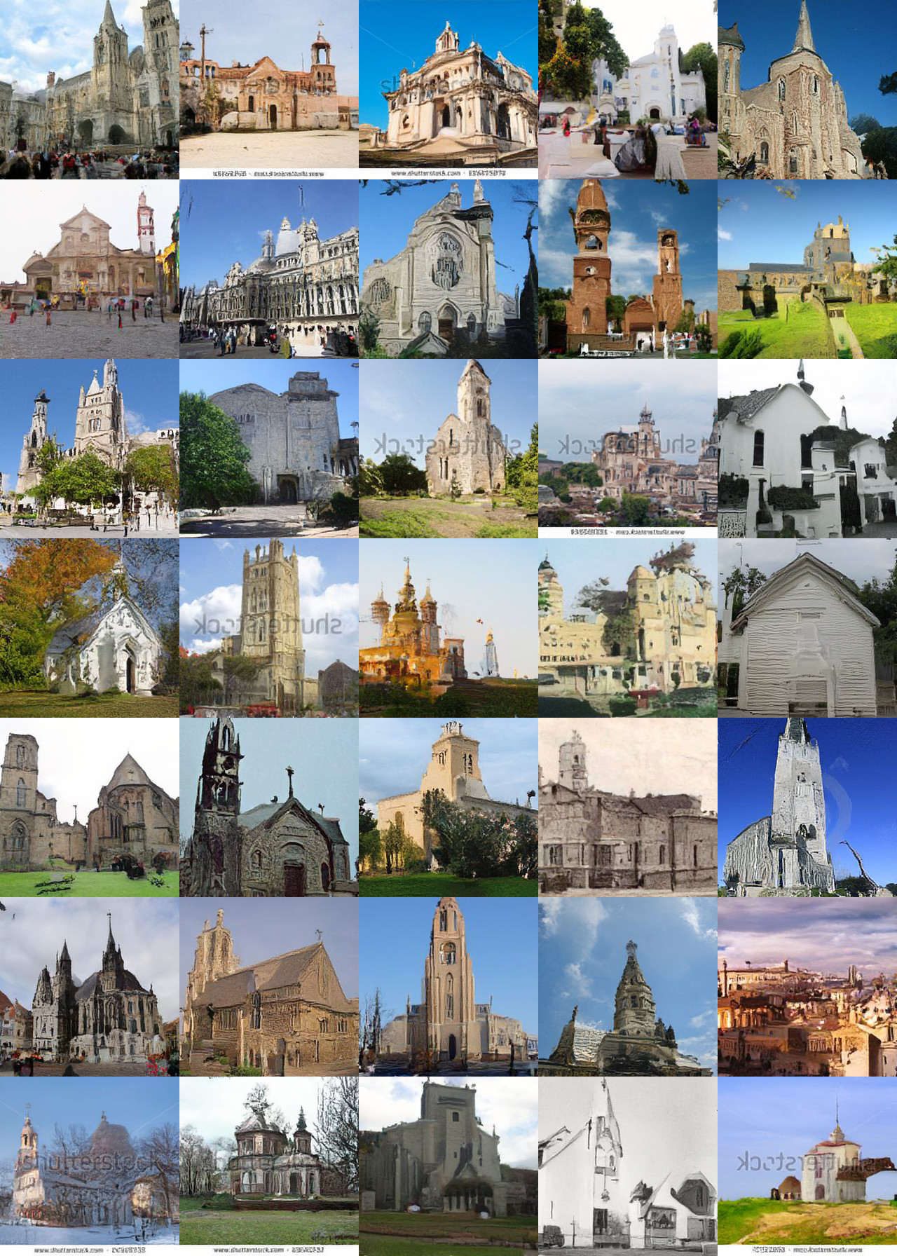
Figure 11: Non-cherry picked, LSUN Church $256\!\times\!256$ samples.

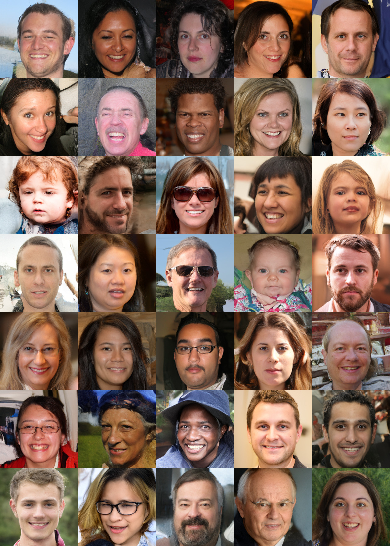
Figure 12: Non-cherry picked, FFHQ $256\!\times\!256$ samples.

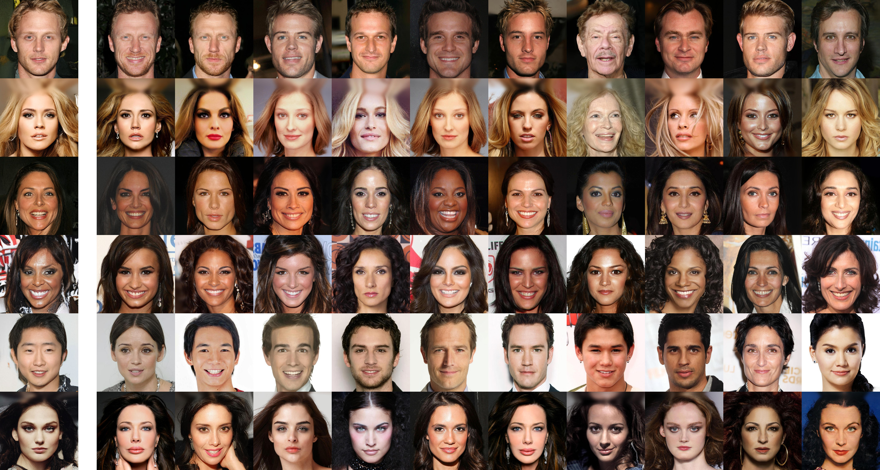
Figure 13: Nearest neighbours for a model trained on CelebA-HQ based on LPIPS distance. The left column contains samples from our model and the right column contains the nearest neighbours in the training set (increasing in distance from left to right)

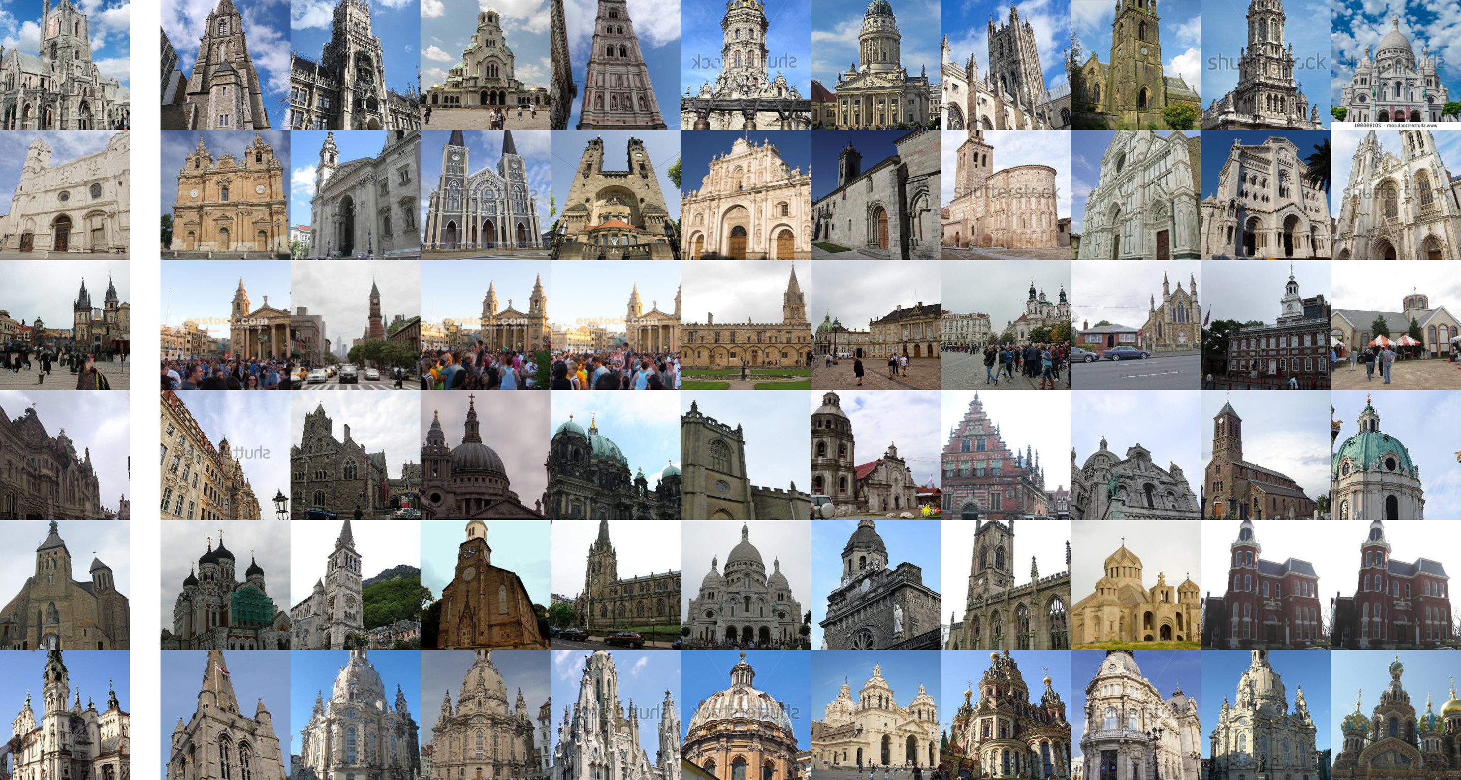
Figure 14: Nearest neighbours for a model trained on LSUN Church based on LPIPS distance. The left column contains samples from our model and the right column contains the nearest neighbours in the training set (increasing in distance from left to right)

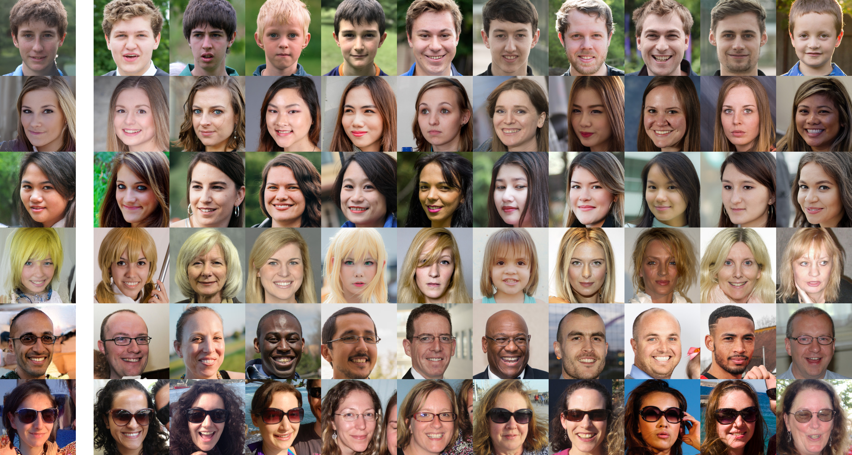
Figure 15: Nearest neighbours for a model trained on FFHQ based on LPIPS distance. The left column contains samples from our model and the right column contains the nearest neighbours in the training set (increasing in distance from left to right)

References

- Albergo et al. [2023] Michael S Albergo, Nicholas M Boffi, and Eric Vanden-Eijnden. Stochastic Interpolants: A Unifying Framework for Flows and Diffusions. arXiv preprint arXiv:2303.08797, 2023.
- Anderson [1982] Brian DO Anderson. Reverse-Time Diffusion Equation Models. Stochastic Processes and their Applications, 12(3):313–326, 1982.
- Anokhin et al. [2021] Ivan Anokhin, Kirill Demochkin, Taras Khakhulin, Gleb Sterkin, Victor Lempitsky, and Denis Korzhenkov. Image Generators with Conditionally-Independent Pixel Synthesis. In Proceedings of the IEEE/CVF Conference on Computer Vision and Pattern Recognition, pages 14278–14287, 2021.
- Ba et al. [2016] Jimmy Lei Ba, Jamie Ryan Kiros, and Geoffrey E Hinton. Layer Normalization. arXiv preprint arXiv:1607.06450, 2016.
- Bishop and Nasrabadi [2006] Christopher M Bishop and Nasser M Nasrabadi. Pattern Recognition and Machine Learning, volume 4. Springer, 2006.
- Bond-Taylor and Willcocks [2021] Sam Bond-Taylor and Chris G Willcocks. Gradient Origin Networks. In International Conference on Learning Representations, 2021.
- Bond-Taylor et al. [2022] Sam Bond-Taylor, Peter Hessey, Hiroshi Sasaki, Toby P Breckon, and Chris G Willcocks. Unleashing Transformers: Parallel Token Prediction with Discrete Absorbing Diffusion for Fast High-Resolution Image Generation from Vector-Quantized Codes. In European Conference on Computer Vision, pages 170–188. Springer, 2022.
- Cao [2021] Shuhao Cao. Choose a Transformer: Fourier or Galerkin. Advances in Neural Information Processing Systems, 34:24924–24940, 2021.
- Chen et al. [2018] Ricky TQ Chen, Yulia Rubanova, Jesse Bettencourt, and David K Duvenaud. Neural Ordinary Differential Equations. Advances in neural information processing systems, 31, 2018.
- Choy et al. [2019] Christopher Choy, JunYoung Gwak, and Silvio Savarese. 4d Spatio-Temporal ConvNets: Minkowski Convolutional Neural Networks. In Proceedings of the IEEE Conference on Computer Vision and Pattern Recognition, pages 3075–3084, 2019.
- Contributors [2022] Spconv Contributors. Spconv: Spatially Sparse Convolution Library. https://github.com/traveller59/spconv, 2022.
- Cotter et al. [2013] SL Cotter, GO Roberts, AM Stuart, and D White. MCMC Methods for Functions: Modifying Old Algorithms to Make Them Faster. Statistical Science, 28(3):424–446, 2013.
- Da Prato [2006] Giuseppe Da Prato. An Introduction to Infinite-Dimensional Analysis. Springer Science & Business Media, 2006.
- Da Prato and Zabczyk [2014] Giuseppe Da Prato and Jerzy Zabczyk. Stochastic Equations in Infinite Dimensions. Cambridge university press, 2014.
- De Bortoli et al. [2021] Valentin De Bortoli, James Thornton, Jeremy Heng, and Arnaud Doucet. Diffusion Schrödinger Bridge with Applications to Score-Based Generative Modeling. Advances in Neural Information Processing Systems, 34:17695–17709, 2021.
- Dockhorn et al. [2022] Tim Dockhorn, Arash Vahdat, and Karsten Kreis. Score-Based Generative Modeling with Critically-Damped Langevin Diffusion. In International Conference on Learning Representations, 2022.
- Du et al. [2021] Yilun Du, Katie Collins, Josh Tenenbaum, and Vincent Sitzmann. Learning Signal-Agnostic Manifolds of Neural Fields. Advances in Neural Information Processing Systems, 34:8320–8331, 2021.
- Dupont et al. [2022a] Emilien Dupont, Hyunjik Kim, SM Ali Eslami, Danilo Jimenez Rezende, and Dan Rosenbaum. From data to functa: Your data point is a function and you can treat it like one. In International Conference on Machine Learning, pages 5694–5725. PMLR, 2022a.
- Dupont et al. [2022b] Emilien Dupont, Yee Whye Teh, and Arnaud Doucet. Generative Models as Distributions of Functions. In International Conference on Artificial Intelligence and Statistics, pages 2989–3015. PMLR, 2022b.
- Dutordoir et al. [2022] Vincent Dutordoir, Alan Saul, Zoubin Ghahramani, and Fergus Simpson. Neural Diffusion Processes. arXiv preprint arXiv:2206.03992, 2022.
- Föllmer and Wakolbinger [1986] H Föllmer and A Wakolbinger. Time Reversal of Infinite-Dimensional Diffusions. Stochastic processes and their applications, 22(1):59–77, 1986.
- Franzese et al. [2023] Giulio Franzese, Simone Rossi, Dario Rossi, Markus Heinonen, Maurizio Filippone, and Pietro Michiardi. Continuous-Time Functional Diffusion Processes. arXiv preprint arXiv:2303.00800, 2023.
- Garnelo et al. [2018] Marta Garnelo, Jonathan Schwarz, Dan Rosenbaum, Fabio Viola, Danilo J Rezende, SM Eslami, and Yee Whye Teh. Neural processes. ICML Workshop, 2018.
- Gawarecki and Mandrekar [2010] Leszek Gawarecki and Vidyadhar Mandrekar. Stochastic Differential Equations in Infinite Dimensions: with Applications to Stochastic Partial Differential Equations. Springer Science & Business Media, 2010.
- Hagemann et al. [2023] Paul Hagemann, Lars Ruthotto, Gabriele Steidl, and Nicole Tianjiao Yang. Multilevel Diffusion: Infinite Dimensional Score-Based Diffusion Models for Image Generation. arXiv preprint arXiv:2303.04772, 2023.
- Heusel et al. [2017] Martin Heusel, Hubert Ramsauer, Thomas Unterthiner, Bernhard Nessler, and Sepp Hochreiter. GANs Trained by a Two Time-Scale Update Rule Converge to a Local Nash Equilibrium. Advances in neural information processing systems, 30, 2017.
- Higdon [2002] Dave Higdon. Space and Space-Time Modeling using Process Convolutions. In Quantitative methods for current environmental issues, pages 37–56. Springer, 2002.
- Ho et al. [2020] Jonathan Ho, Ajay Jain, and Pieter Abbeel. Denoising Diffusion Probabilistic Models. Advances in Neural Information Processing Systems, 33:6840–6851, 2020.
- Ho et al. [2022a] Jonathan Ho, Chitwan Saharia, William Chan, David J Fleet, Mohammad Norouzi, and Tim Salimans. Cascaded Diffusion Models for High Fidelity Image Generation. J. Mach. Learn. Res., 23(47):1–33, 2022a.
- Ho et al. [2022b] Jonathan Ho, Tim Salimans, Alexey A Gritsenko, William Chan, Mohammad Norouzi, and David J Fleet. Video Diffusion Models. In Advances in Neural Information Processing Systems, 2022b.
- Hoogeboom and Salimans [2023] Emiel Hoogeboom and Tim Salimans. Blurring Diffusion Models. In International Conference on Learning Representations, 2023.
- Hoogeboom et al. [2023] Emiel Hoogeboom, Jonathan Heek, and Tim Salimans. Simple Diffusion: End-to-End Diffusion for High Resolution Images. arXiv preprint arXiv:2301.11093, 2023.
- Hyvärinen [2005] Aapo Hyvärinen. Estimation of Non-Normalized Statistical Models by Score Matching. Journal of Machine Learning Research, 6(4), 2005.
- Jabri et al. [2022] Allan Jabri, David Fleet, and Ting Chen. Scalable Adaptive Computation for Iterative Generation. arXiv preprint arXiv:2212.11972, 2022.
- Karras et al. [2018] Tero Karras, Timo Aila, Samuli Laine, and Jaakko Lehtinen. Progressive Growing of GANs for Improved Quality, Stability, and Variation. In International Conference on Learning Representations, 2018.
- Karras et al. [2019] Tero Karras, Samuli Laine, and Timo Aila. A Style-Based Generator Architecture for Generative Adversarial Networks. In Proceedings of the IEEE/CVF Conference on Computer Vision and Pattern Recognition, pages 4401–4410, 2019.
- Karras et al. [2020] Tero Karras, Samuli Laine, Miika Aittala, Janne Hellsten, Jaakko Lehtinen, and Timo Aila. Analyzing and Improving the Image Quality of StyleGAN. In Proceedings of the IEEE/CVF conference on computer vision and pattern recognition, pages 8110–8119, 2020.
- Kingma and Ba [2015] Diederik P Kingma and Jimmy Ba. Adam: A Method for Stochastic Optimization. In International Conference on Learning Representations, 2015.
- Kovachki et al. [2021] Nikola Kovachki, Zongyi Li, Burigede Liu, Kamyar Azizzadenesheli, Kaushik Bhattacharya, Andrew Stuart, and Anima Anandkumar. Neural Operator: Learning Maps Between Function Spaces. arXiv preprint arXiv:2108.08481, 2021.
- Kynkäänniemi et al. [2023] Tuomas Kynkäänniemi, Tero Karras, Miika Aittala, Timo Aila, and Jaakko Lehtinen. The Role of ImageNet Classes in Fréchet Inception Distance. 2023.
- Li et al. [2020] Zongyi Li, Nikola Kovachki, Kamyar Azizzadenesheli, Burigede Liu, Kaushik Bhattacharya, Andrew Stuart, and Anima Anandkumar. Neural Operator: Graph Kernel Network for Partial Differential Equations. arXiv preprint arXiv:2003.03485, 2020.
- Li et al. [2021] Zongyi Li, Nikola Borislavov Kovachki, Kamyar Azizzadenesheli, Kaushik Bhattacharya, Andrew Stuart, Anima Anandkumar, et al. Fourier Neural Operator for Parametric Partial Differential Equations. In International Conference on Learning Representations, 2021.
- Lim et al. [2023] Jae Hyun Lim, Nikola B Kovachki, Ricardo Baptista, Christopher Beckham, Kamyar Azizzadenesheli, Jean Kossaifi, Vikram Voleti, Jiaming Song, Karsten Kreis, Jan Kautz, et al. Score-Based Diffusion Models in Function Space. arXiv preprint arXiv:2302.07400, 2023.
- Liu et al. [2022] Zhuang Liu, Hanzi Mao, Chao-Yuan Wu, Christoph Feichtenhofer, Trevor Darrell, and Saining Xie. A ConvNet for the 2020s. In Proceedings of the IEEE/CVF Conference on Computer Vision and Pattern Recognition, pages 11976–11986, 2022.
- Lu et al. [2022] Cheng Lu, Yuhao Zhou, Fan Bao, Jianfei Chen, Chongxuan Li, and Jun Zhu. Dpm-Solver: A Fast ODE Solver for Diffusion Probabilistic Model Sampling in Around 10 Steps. In Advances in Neural Information Processing Systems, 2022.
- Nichol and Dhariwal [2021] Alexander Quinn Nichol and Prafulla Dhariwal. Improved Denoising Diffusion Probabilistic Models. In International Conference on Machine Learning, pages 8162–8171. PMLR, 2021.
- Pinski et al. [2015] Francis J Pinski, Gideon Simpson, Andrew M Stuart, and Hendrik Weber. Kullback–Leibler Approximation for Probability Measures on Infinite Dimensional Spaces. SIAM Journal on Mathematical Analysis, 47(6):4091–4122, 2015.
- Preechakul et al. [2022] Konpat Preechakul, Nattanat Chatthee, Suttisak Wizadwongsa, and Supasorn Suwajanakorn. Diffusion Autoencoders: Toward a Meaningful and Decodable Representation. In Proceedings of the IEEE/CVF Conference on Computer Vision and Pattern Recognition, pages 10619–10629, 2022.
- Qi et al. [2017] Charles Ruizhongtai Qi, Li Yi, Hao Su, and Leonidas J Guibas. PointNet++: Deep Hierarchical Feature Learning on Point Sets in a Metric Space. Advances in neural information processing systems, 30, 2017.
- Radford et al. [2021] Alec Radford, Jong Wook Kim, Chris Hallacy, Aditya Ramesh, Gabriel Goh, Sandhini Agarwal, Girish Sastry, Amanda Askell, Pamela Mishkin, Jack Clark, et al. Learning Transferable Visual Models from Natural Language Supervision. In International Conference on Machine Learning, pages 8748–8763. PMLR, 2021.
- Rahman et al. [2022] Md Ashiqur Rahman, Zachary E Ross, and Kamyar Azizzadenesheli. U-NO: U-Shaped Neural Operators. arXiv preprint arXiv:2204.11127, 2022.
- Rezende and Mohamed [2015] Danilo Rezende and Shakir Mohamed. Variational Inference with Normalizing Flows. In International Conference on Machine Learning, pages 1530–1538. PMLR, 2015.
- Rissanen et al. [2023] Severi Rissanen, Markus Heinonen, and Arno Solin. Generative Modelling with Inverse Heat Dissipation. In International Conference on Learning Representations, 2023.
- Rombach et al. [2022] Robin Rombach, Andreas Blattmann, Dominik Lorenz, Patrick Esser, and Björn Ommer. High-Resolution Image Synthesis with Latent Diffusion Models. In Proceedings of the IEEE/CVF Conference on Computer Vision and Pattern Recognition, pages 10684–10695, 2022.
- Romero et al. [2022] David W Romero, Robert-Jan Bruintjes, Jakub Mikolaj Tomczak, Erik J Bekkers, Mark Hoogendoorn, and Jan van Gemert. Flexconv: Continuous kernel convolutions with differentiable kernel sizes. In International Conference on Learning Representations, 2022.
- Ronneberger et al. [2015] Olaf Ronneberger, Philipp Fischer, and Thomas Brox. U-Net: Convolutional Networks for Biomedical Image Segmentation. In International Conference on Medical image computing and computer-assisted intervention, pages 234–241. Springer, 2015.
- Salimans and Ho [2022] Tim Salimans and Jonathan Ho. Progressive Distillation for Fast Sampling of Diffusion Models. In International Conference on Learning Representations, 2022.
- Singh et al. [2023] Rajhans Singh, Ankita Shukla, and Pavan Turaga. Polynomial Implicit Neural Representations For Large Diverse Datasets. arXiv preprint arXiv:2301.11093, 2023.
- Sitzmann et al. [2020] Vincent Sitzmann, Julien Martel, Alexander Bergman, David Lindell, and Gordon Wetzstein. Implicit Neural Representations with Periodic Activation Functions. Advances in Neural Information Processing Systems, 33:7462–7473, 2020.
- Sohl-Dickstein et al. [2015] Jascha Sohl-Dickstein, Eric Weiss, Niru Maheswaranathan, and Surya Ganguli. Deep Unsupervised Learning using Nonequilibrium Thermodynamics. In International Conference on Machine Learning, pages 2256–2265. PMLR, 2015.
- Song et al. [2021a] Jiaming Song, Chenlin Meng, and Stefano Ermon. Denoising Diffusion Implicit Models. In International Conference on Learning Representations, 2021a.
- Song and Ermon [2019] Yang Song and Stefano Ermon. Generative Modeling by Estimating Gradients of the Data Distribution. Advances in Neural Information Processing Systems, 32, 2019.
- Song et al. [2021b] Yang Song, Jascha Sohl-Dickstein, Diederik P Kingma, Abhishek Kumar, Stefano Ermon, and Ben Poole. Score-Based Generative Modeling through Stochastic Differential Equations. In International Conference on Learning Representations, 2021b.
- Song et al. [2023] Yang Song, Prafulla Dhariwal, Mark Chen, and Ilya Sutskever. Consistency Models. arXiv preprint arXiv:2303.01469, 2023.
- Tang et al. [2022] Haotian Tang, Zhijian Liu, Xiuyu Li, Yujun Lin, and Song Han. TorchSparse: Efficient Point Cloud Inference Engine. In Conference on Machine Learning and Systems (MLSys), 2022.
- Tolstikhin et al. [2021] Ilya O Tolstikhin, Neil Houlsby, Alexander Kolesnikov, Lucas Beyer, Xiaohua Zhai, Thomas Unterthiner, Jessica Yung, Andreas Steiner, Daniel Keysers, Jakob Uszkoreit, et al. MLP-Mixer: An All-MLP Architecture for Vision. Advances in Neural Information Processing Systems, 34:24261–24272, 2021.
- Vincent [2011] Pascal Vincent. A Connection Between Score Matching and Denoising Autoencoders. Neural computation, 23(7):1661–1674, 2011.
- Wang and Golland [2022] Clinton Wang and Polina Golland. Discretization Invariant Learning on Neural Fields. In arXiv preprint arXiv:2206.01178, 2022.
- Xie et al. [2022] Yiheng Xie, Towaki Takikawa, Shunsuke Saito, Or Litany, Shiqin Yan, Numair Khan, Federico Tombari, James Tompkin, Vincent Sitzmann, and Srinath Sridhar. Neural Fields in Visual Computing and Beyond. In Computer Graphics Forum, volume 41, pages 641–676. Wiley Online Library, 2022.
- Yu et al. [2015] Fisher Yu, Yinda Zhang, Shuran Song, Ari Seff, and Jianxiong Xiao. LSUN: Construction of a Large-scale Image Dataset using Deep Learning with Humans in the Loop. arXiv preprint arXiv:1506.03365, 2015.
- Zhang et al. [2022] Bowen Zhang, Shuyang Gu, Bo Zhang, Jianmin Bao, Dong Chen, Fang Wen, Yong Wang, and Baining Guo. StyleSwin: Transformer-Based GAN for High-Resolution Image Generation. In Proceedings of the IEEE/CVF Conference on Computer Vision and Pattern Recognition, pages 11304–11314, 2022.
- Zhang et al. [2018] Richard Zhang, Phillip Isola, Alexei A Efros, Eli Shechtman, and Oliver Wang. The Unreasonable Effectiveness of Deep Features as a Perceptual Metric. In Proceedings of the IEEE conference on computer vision and pattern recognition, pages 586–595, 2018.
- Zhuang et al. [2023] Peiye Zhuang, Samira Abnar, Jiatao Gu, Alex Schwing, Joshua M Susskind, and Miguel Ángel Bautista. Diffusion Probabilistic Fields. In International Conference on Learning Representations, 2023.