Hydrodynamical constraints on bubble wall velocity

Abstract

Terminal velocity reached by bubble walls in first order phase transitions is an important parameter determining both primordial gravitational-wave spectrum and production of baryon asymmetry in models of electroweak baryogenesis. We developed a numerical code to study the real-time evolution of expanding bubbles and investigate how their walls reach stationary states. Our results agree with profiles obtained within the so-called bag model with very good accuracy, however, not all such solutions are stable and realised in dynamical systems. Depending on the exact shape of the potential there is always a range of wall velocities where no steady state solutions exist. This behaviour in deflagrations was explained by hydrodynamical obstruction where solutions that would heat the plasma outside the wall above the critical temperature and cause local symmetry restoration are forbidden. For even more affected hybrid solutions causes are less straight forward, however, we provide a simple numerical fit allowing one to verify if a solution with a given velocity is allowed simply by computing the ratio of the nucleation temperature to the critical one for the potential in question.

1 Introduction

Phase transitions are a common feature of particle physics models. If they are first order they can open a path to numerous phenomena such as generation of the baryon asymmetry Kuzmin:1985mm ; Cohen:1993nk ; Rubakov:1996vz ; Morrissey:2012db and production of a stochastic background of GWs Caprini:2015zlo ; Caprini:2019egz ; AEDGE:2019nxb ; Badurina:2021rgt . Significant progress has been made recently in understanding fine details of the dynamics of such transitions necessary to describe the intricate relation between these possibilities Cline:2020jre ; Laurent:2020gpg ; Cline:2021iff ; Dorsch:2021ubz ; Cline:2021dkf ; Lewicki:2021pgr ; Dorsch:2021nje ; Laurent:2022jrs ; Ellis:2022lft . Despite that evaluation, the bubble-wall velocity in the stationary state remains to be one of the more problematic issues. Given its impact both on the amplitude of the gravitational-wave signal as well as the production of the baryon asymmetry this has to be solved to finally pinpoint the interplay between the two signals.

Contrary to nucleation temperature or transition strength, the wall velocity is not a straightforward consequence of the shape of the effective potential. The standard WKB method of computing the velocity involves solving a set of Boltzmann equations in the vicinity of the bubble wall in order to find the friction the plasma will enact on the expanding wall. However, the result still crucially relies on the hydrodynamical solution for the plasma profile No:2011fi ; Cline:2021iff ; Lewicki:2021pgr . It is a standard practice to use the plasma behaviour obtained in the bag model in these studies. The obvious drawback of this approach is that the bag equation of state (EOS) inherently neglects all knowledge of the potential except the energy difference between its minima Espinosa:2010hh .

In this work, we investigate the impact of detailed features of the potential on hydrodynamical solutions for the plasma. To this end, we perform lattice simulations tracking the real-time evolution of the bubble-wall profiles. We focus on the hydrodynamical solutions for a single expanding bubble using novel methods that allow us to resolve shocks properly and prevent the appearance of unphysical artefacts. Our method involves algebraic flux-corrected transport (FCT), described in Kuzmin:2002 ; Kuzmin:2003 ; Moller:2013 ; Kuzmin:2021 with an improved version of Zalesak’s limiter Zalesak:1979 . This allows us to study in detail how the system reaches a stationary state and compare these late-time profiles with analytical approximations. We take a closer look at the problem of hydrodynamical obstruction and find a large class of unstable solutions that constitute a forbidden range for bubble-wall velocities below the Jouguet velocity.

The paper is structured as follows. In section 2 we discuss the details of the set-up including the exact model and form of equations of motions that govern its evolution as well as analytical approximations for the solution. Sec. 3 is devoted to the results of our simulations including the dependence of the solutions on the temperature and vacuum expectation value (vev) of the field. Here we also give a simple fit allowing one to approximate the forbidden region in any potential. We conclude in section 4. Appendix A contains finer details of our numerical set-up.

2 Modeling

In this section, we discuss details of the model we will work with as well as its analytically solvable simplification. We derive equations of motion for the scalar field coupled to the perfect fluid and discuss nucleation conditions which we later use to initialize the evolution. Finally, we briefly discuss the steady state description known as the bag model.

2.1 Scalar field coupled to perfect fluid

In this work, we investigate a well-known system consisting of the scalar field $\phi$ coupled to the perfect fluid described by its temperature $T$ and local flow four-velocity $u$ Ignatius:1993qn ; Kurki-Suonio:1995yaf ; Kurki-Suonio:1996wfr ; Hindmarsh:2013xza ; Hindmarsh:2015qta . The equation of state is given by

$$\epsilon(\phi,T) =3aT^{4}+V(\phi,T)-T\frac{\partial V}{\partial T}\,,$$ (1)

$$p(\phi,T) =aT^{4}-V(\phi,T)\,,$$ (2)

where $a=(\pi^{2}/90)g_{*}$ and $w\equiv\epsilon+p$. For the effective potential $V(\phi,T)$ we use a simple polynomial potential augmented with high-temperature corrections parameterized as

$$V(\phi,T)=\frac{1}{2}\gamma(T^{2}-T_{0}^{2})\phi^{2}-\frac{1}{3}\delta T\phi^{3}+\frac{1}{4}\lambda\phi^{4}\,.$$ (3)

The energy-momentum tensor of the system is a sum of energy-momentum tensors for the field and the fluid:

$$T^{\mu\nu}_{\textrm{field}} =\partial^{\mu}\phi\partial^{\nu}\phi-g^{\mu\nu}\left(\frac{1}{2}\partial_{\alpha}\phi\partial^{\alpha}\phi\right)\,,$$ (4)

$$T^{\mu\nu}_{\textrm{fluid}} =wu^{\mu}u^{\nu}+g^{\mu\nu}p\,,$$ (5)

where $p$ is the pressure of the perfect fluid.

We use spherical coordinates in space as they capture the symmetry of a single growing bubble that we intend to simulate . The line element $ds$ for the flat space-time takes the following form in these coordinates:

$$ds^{2}=-dt^{2}+dr^{2}+r^{2}\left(d\theta^{2}+\sin^{2}{\theta}d\varphi^{2}\right)\,.$$ (6)

The energy-momentum tensor of the system is conserved $(\nabla_{\mu}T^{\mu\nu}=0)$, however, both contributions are not conserved separately due to extra coupling term parameterised by the effective coupling of the fluid and scalar:

$$\nabla_{\mu}T^{\mu\nu}_{\textrm{field}} =\frac{\partial V}{\partial\phi}\partial^{\nu}\phi+\eta u^{\mu}\partial_{\mu}\phi\partial^{\nu}\phi\,,$$ (7)

$$\nabla_{\mu}T^{\mu\nu}_{\textrm{fluid}} =-\frac{\partial V}{\partial\phi}\partial^{\nu}\phi-\eta u^{\mu}\partial_{\mu}\phi\partial^{\nu}\phi\,,$$ (8)

where $\eta$ is a constant parametrizing strength of this interaction. The left-hand side of the equation (7) contains wave equation in spherical coordinates and leads to the equation of motion

$$-\partial_{t}^{2}\phi+\frac{1}{r^{2}}\partial_{r}(r^{2}\partial_{r}\phi)-\frac{\partial V}{\partial\phi}=\eta\gamma(\partial_{t}\phi+v\partial_{r}\phi)\,.$$ (9)

Due to the spherical symmetry of our problem, the four-velocity of the perfect fluid takes the form $u=(\gamma,\gamma v,0,0)^{T}$ with $\gamma:=(1-v^{2})^{-1}$. We will determine the equations governing the evolution of two parameters $v$ and $p$ considering time ($\nu=0$) and radial component ($\nu=1$) of eq. (8):

$$\nabla_{\mu}T^{\mu 0}_{\textrm{fluid}} =\nabla_{\mu}\left(wu^{\mu}u^{0}+g^{\mu 0}p\right)=\partial_{t}(w\gamma^{2}-p)+\frac{1}{r^{2}}\partial_{r}(r^{2}w\gamma^{2}v)\,,$$ (10a)

$$\nabla_{\mu}T^{\mu 1}_{\textrm{fluid}} =\nabla_{\mu}\left(wu^{\mu}u^{1}+g^{\mu 1}p\right)=\partial_{t}(w\gamma^{2}v)+\frac{1}{r^{2}}\partial_{r}\left(r^{2}w\gamma^{2}v^{2}\right)+\partial_{r}p\,.$$ (10b)

Introducing new variables $Z:=w\gamma^{2}v$ and $\tau:=w\gamma^{2}-p$ we get

$$\partial_{t}\tau+\frac{1}{r^{2}}\partial_{r}(r^{2}(\tau+p)v) =\frac{\partial V}{\partial\phi}\partial_{t}\phi+\eta\gamma(\partial_{t}\phi+v\partial_{r}\phi)\partial_{t}\phi\,,$$ (11a)

$$\partial_{t}Z+\frac{1}{r^{2}}\partial_{r}\left(r^{2}Zv\right)+\partial_{r}p =-\frac{\partial V}{\partial\phi}\partial_{r}\phi-\eta\gamma(\partial_{t}\phi+v\partial_{r}\phi)\partial_{r}\phi\,.$$ (11b)

The final step needed to evolve the system numerically is to discretize and solve system of equations presented above. All technical details of this procedure are described in Appendix A.

2.2 Nucleation of the bubbles

The system we are interested in consists of a single bubble growing in the fluid background. Each of our simulations is initialized with a recently nucleated bubble of the scalar field. Probability of tunneling at temperature $T$ is computed from the bubble nucleation rate Coleman:1977py ; Callan:1977pt ; Linde:1980tt ; Linde:1981zj

$$\Gamma(T)=A(T)\textrm{e}^{-S}\,.$$ (12)

For tunneling in finite temperatures the Euclidean action $S=\frac{S_{3}}{T}$ and $A(T)=T^{4}\left(\frac{S_{3}}{2\pi T}\right)^{\frac{3}{2}}$. In order to obtain the critical bubble, one needs to find the nucleation temperature $T_{n}$ at which the probability of a true vacuum bubble forming within a horizon radius becomes significant Ellis:2018mja

$$N(T_{n})=\int_{T_{n}}^{T_{c}}\frac{dT}{T}\frac{\Gamma(T)}{H(T)^{4}}\approx 1,$$ (13)

where $T_{c}$ denotes the critical temperature in which both minima are degenerate. Assuming $H(t)\approx$ const, this condition reduces to

$$\frac{S_{3}}{T_{n}}\approx 4\log\left(\frac{T_{n}}{H}\right),$$ (14)

which for temperatures around the electroweak scale gives $S_{3}/T_{n}\approx 140$ Caprini:2019egz . In the case of polynomial potentials, the critical action can be easily evaluated using the semi-analytical approximation described in Appendix B.

An important parameter characterizing transition strength is the amount of the vacuum energy released in the transition $\alpha$, normalized to the energy of the radiation bath $\rho_{r}$. In the fluid approximation, it can be defined as

$$\alpha_{\theta}=\frac{\theta_{s}-\theta_{b}}{\rho_{r}}\Big{|}_{T=T_{n}},$$ (15)

where $\theta$ is the trace anomaly in the symmetric (s) and broken (b) phase, given by the expression

$$\theta=\frac{1}{4}(\epsilon-3p).$$ (16)

Note, that such a definition of the trace anomaly applied to the equation of state (1)-(2) corresponds to a frequently used definition of $\alpha=\frac{1}{\rho_{r}}\left(\Delta V-\frac{T}{4}\Delta\frac{\partial V}{\partial T}\right)$ Hindmarsh:2017gnf ; LISACosmologyWorkingGroup:2022jok .

2.3 Analytical approximation: bag model

A simple model explaining analytically many important features of the late-time evolution is the bag model Espinosa:2010hh . It assumes that the cosmic plasma coexists in two phases:

• Symmetric phase outside the bubble

• Broken phase inside the bubble.

However, it does not include the scalar field explicitly. The equation of state in the bag model reads

$$\epsilon_{s} =3a_{s}T_{s}^{4}+\theta_{s} \epsilon_{b} =3a_{b}T_{b}^{4}+\theta_{b}$$ (17)

$$p_{s} =a_{s}T_{s}^{4}-\theta_{s} p_{b} =a_{b}T_{b}^{4}-\theta_{b},$$ (18)

where $\theta_{s}$ and $\theta_{b}$ are constants and usually one assumes $\theta_{b}=0$. Therefore the strength of the transition can be consistently defined with the equation (15). Assuming that the plasma is locally in equilibrium, the energy-momentum tensor can be parameterized for the perfect fluid as:

$$T^{\mu\nu}=wu^{\mu}u^{\nu}-g^{\mu\nu}p.$$ (19)

Conservation of $T^{\mu\nu}$ along the flow and its projection perpendicular to the flow respectively give

$$\partial_{\mu}(u^{\mu}w)-u_{\mu}\partial^{\mu}p =0,$$ (20)

$$\bar{u}^{\nu}u^{\mu}w\partial_{\mu}u_{\nu}-\bar{u}^{\nu}\partial_{\mu}p =0,$$ (21)

with $\bar{u}_{\mu}u^{\mu}=0$ and $\bar{u}^{2}=-1$. As there is no characteristic distance scale in the problem, the solution should depend only on the self-similar variable $\xi=r/t$, where $r$ denotes the distance from the center of the bubble and $t$ is the time since nucleation. Changing the variables, equations (20) and (21) take the form

$$(\xi-v)\frac{\partial_{\xi}\epsilon}{w} =2\frac{v}{\xi}+[1-\gamma^{2}v(\xi-v)]\partial_{\xi}v,$$ (22)

$$(1-v\xi)\frac{\partial_{\xi}p}{w} =\gamma^{2}(\xi-v)\partial_{\xi}v$$ (23)

and using the definition of the speed of sound in the plasma $c_{s}\equiv\frac{\textrm{d}p}{dT}/\frac{\textrm{d}\epsilon}{dT}$ can be combined into the single equation describing the plasma velocity profile $v(\xi)$ in the frame of the bubble center

$$2\frac{v}{\xi}=\gamma^{2}(1-v\xi)\left[\frac{\mu^{2}}{c_{s}^{2}}-1\right]\partial_{\xi}v,$$ (24)

with $\mu=\frac{\xi-v}{1-\xi v}$ denoting the Lorentz-transformed fluid velocity. Solutions of the equation (24) in general depend only on the transition strength $\alpha$ and bubble-wall velocity in the stationary state $\xi_{w}$. In a similar way, analytical profiles for the enthalpy $w$, temperature $T$ and other thermodynamical quantities can be obtained. Later we will refer to them to compare the results of our simulations with the analytical solutions. Detailed derivations are described in Espinosa:2010hh ; Hindmarsh:2019phv ; Ellis:2020awk ; Lewicki:2021pgr . In general, there exist three types of the bubble-wall profiles:

1. Deflagrations are the solutions with subsonic bubble-wall velocity $\xi_{w}$. In such a case, expanding bubble pushes the plasma in front of it, while behind the bubble wall plasma remains at rest. Typically value of $v$ decreases with $\xi$ in the range $[\xi_{w},c_{s}]$ and vanishes for $\xi>c_{s}$. Therefore a shock front at $\xi=c_{s}$ may appear if the transition is strong enough.

2. Detonations are supersonic solutions, for which bubble-wall velocity exceeds Jouget velocity. In this type of profile, the wall hits plasma which remains at rest in front of the bubble. As fluid enters the broken phase, it slows down smoothly and reaches zero at $\xi=c_{s}$.

3. Hybrids are combinations of the two types mentioned above. They are realised for $\xi_{w}\in[c_{s},c_{J}]$ and possess features of deflagrations (shock front in front of the wall) and detonations (non-zero plasma velocity behind the wall known as a rarefaction wave).

All three types of solutions are schematically depicted in Fig. 1. The Jouget velocity $c_{J}$ at which the shell around the bubble disappears and the solution shifts from hybrid to detonation is given by Chapman-Jouguet condition Steinhardt:1981ct ; Lewicki:2021pgr

$$c_{J}=\frac{1}{\sqrt{3}}\frac{1+\sqrt{1+3\alpha^{2}+2\alpha}}{1+\alpha}.$$ (25)

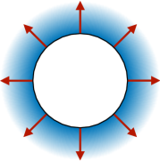
(a) deflagration: $\xi_{w}<c_{s}$

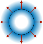
(b) hybrid: $c_{s}<\xi_{w}<c_{J}$

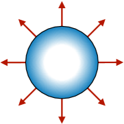
(c) detonation: $c_{J}<\xi_{w}$

Figure 1: Schematic representation of three different types of expanding bubbles. Colour saturation denotes the value of the plasma velocity, while black circles represent the position of the bubble wall.

3 Results from numerical simulations

In this section, we will discuss the results of our numerical simulations. We start with the validation of our method on two benchmark points already studied in the past. Next, we move on to our main results on existence of the gap in the allowed fluid solutions impacting the realisation of hybrids. We discuss the role of key parameters that is the temperature of the transition and the vev of the field. Every simulation is performed on the lattice with $\delta r=0.01$ GeV^-1 and $\delta t=0.001$ GeV^-1. The time duration of the evolution is large enough to asymptotically achieve stationary states and is set to $t_{max}=120$ GeV^-1. Similarly, the physical size of the lattice is fixed as $R=ct_{max}$ which is large enough to prevent reaching the boundaries by the bubbles, since they expand subluminally. We initialize each simulation with the recently nucleated bubble, fixing the field configuration to the critical profile and setting $T=T_{n}$ and $v=0$ everywhere. The value of the friction parameter depends on the field content of the model and as a result, we keep it as a free parameter. We logarithmically vary it in the range $\eta/T_{c}\in[0.01,1]$, independently checking around 75 values for every scalar potential which is enough to map all the allowed classes of solutions in each case.

3.1 Benchmark points

In order to evaluate the performance of our code, we initialized runs with two benchmark points that were already studied in similar a context Hindmarsh:2013xza . All important parameters characterizing these models are summarized in Table 1.

Model	$T_{c}$ [GeV]	$T_{0}$ [GeV]	$\gamma$	$\delta$	$\lambda$	$T_{n}$ [GeV]	$\alpha_{\theta}$
$M_{1}$	$100$	$\frac{100}{\sqrt{2}}$	$\frac{1}{18}$	$\frac{\sqrt{10}}{72}$	$\frac{10}{648}$	$86$	0.005
$M_{2}$	$100$	$\frac{100}{\sqrt{2}}$	$\frac{2}{18}$	$\frac{\sqrt{10}}{72}$	$\frac{5}{648}$	$80$	0.05

Table 1: Model parameters for the benchmark points

For both of them, we perform a scan with respect to the friction parameter $\eta$, which is the only free parameter. In accordance with previous studies, steady-state wall velocity $\xi_{w}$ grows as the friction becomes smaller Kurki-Suonio:1996wfr . The general shape of this correspondence was also confirmed, however, the exact form of the curve depends on the choice of the potential parameter and will be discussed later in this paper.

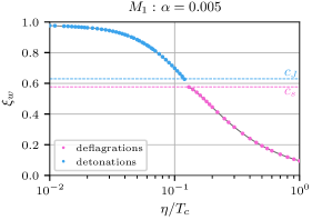
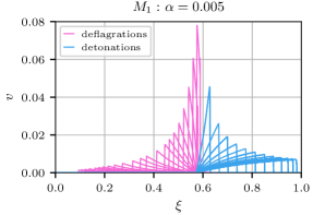
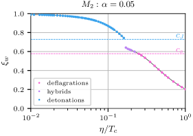
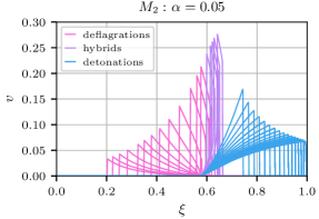
Figure 2: Relation between the friction parameter $\eta$ and bubble-wall velocity in the stationary state $\xi_{w}$ (left panels). Overview of the corresponding velocity profiles for each point (right panels). The first row corresponds to the weaker transition ($M_{1}$), while the second to the stronger one ($M_{2}$).

For the stronger transition $(M_{2})$ we managed to obtain all three types of solutions, while for the weaker one $(M_{1})$ no hybrids were realised. We, therefore, confirm the presence of the velocity gap in the region where one expects hybrid profiles. Such a gap appears in both cases, covering the whole $\xi_{w}\in[c_{s},c_{J}]$ range for $M_{1}$ and allowing to continue deflagration branch towards solutions with supersonic wall velocity for $M_{2}$. The details of this phenomenon were not well understood so far and constitute the focus of our interest in the next section. Results of the scan are presented in Fig 2.

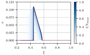
(a) deflagration: $\xi_{w}=0.45$, velocity profile

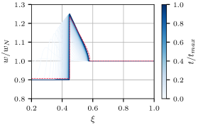
(b) deflagration: $\xi_{w}=0.45$, enthaply profile

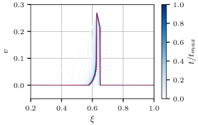
(c) hybrid: $\xi_{w}=0.63$, velocity profile

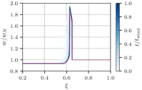
(d) hybrid: $\xi_{w}=0.63$, enthalpy profile

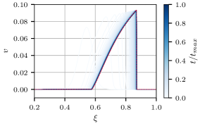
(e) detonation: $\xi_{w}=0.87$, velocity profile

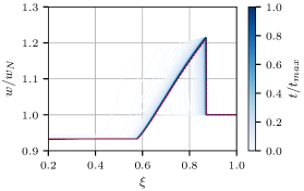
(f) detonation: $\xi_{w}=0.87$, enthalpy profile

Figure 3: Time evolution of the plasma shell profiles for plasma velocity $v$ and enthalpy $w$ as functions of the self-similar variable $\xi=r/t$. In general, all three types of solutions were found: deflagrations (first row), hybrids (second row) and detonations (third row). Different shades of blue correspond with the time flow. Profiles evolve towards stationary states represented by darker colours. Red, dashed lines denote analytical profiles obtained within the bag model.

The shapes of stationary profiles are in very good agreement with the predictions of the bag model . The comparison of the results of our simulations and the analytical profiles for three representative examples is shown in Fig. 3. As one can see, we managed to resolve the shocks and reproduce the form of hybrids with very good accuracy, which typically was challenging in previously existing results involving dynamical codes.

3.2 Dependence on the vacuum expectation value

As shown in the previous section, the exact form of the relation between the friction $\eta$ and the terminal wall velocity $\xi_{w}$, in general, depends on the parameters of the potential. In order to check the dependence on the vacuum expectation value of the scalar field, besides the transition strength $\alpha_{\theta}$ we fixed also nucleation temperature $T_{n}/T_{c}$ and check different realisations of such transitions. Fig. 4 shows that as $\eta\sim\phi^{-1}$, field value in the true vacuum $v_{0}$ fully determines the position of the gap in terms of friction parameter $\eta$. Therefore we conclude that the shape of the $\xi_{w}(\eta)$ relation can be completely explained within terms of $\alpha_{\theta}$ and $T_{n}/T_{c}$ exclusively. Moreover, this dependence should be universal for a much wider class of models involving polynomial potentials, as it does not explicitly involve any model-dependent couplings.

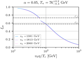
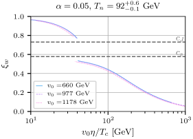
Figure 4: Relation between the friction parameter $\eta$ and bubble-wall velocity in the stationary state $\xi_{w}$ for the fixed nucleation temperature $T_{n}=76$ GeV (left panel) and $T_{n}=92$ GeV (right panel). Different colours represent different positions of the true vacuum.

3.3 Dependence on the temperature

As we have already shown the exact form of the $\xi_{w}(\eta)$ relation is not unique and depends not only on the strength of the transition $\alpha$, but also on other parameters defining the scalar potential. To illustrate this, we study a set of different potentials for which $\alpha_{\theta}$ and $T_{c}$ are fixed, however, the parameters in the potential are chosen such that they predict different nucleation temperatures $T_{n}$. Relations between $\eta$ and $\xi_{w}$ for $\alpha_{\theta}\in\{0.05,0.1\}$ and a range of $T_{n}$ are shown in Fig 5 (left panels).

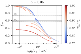
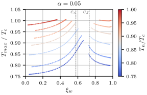
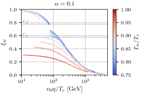
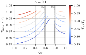
Figure 5: Relation between the friction parameter $\eta$ and bubble-wall velocity in the stationary state $\xi_{w}$ (left panels) and the maximum of the plasma temperature along the profile (right panels). Potentials are chosen such that the strength of the transition is fixed to $\alpha_{\theta}=0.05$ (upper row) and $\alpha_{\theta}=0.1$ (lower row). The value of the nucleation temperature $T_{n}$ is encoded with the colour.

We can see that higher nucleation temperatures lead to a wider velocity gap, while for lower temperatures, almost the entire range of wall velocities can be covered. Note that nucleation temperatures very close to the critical temperature limit the bubble wall velocity for both deflagrations and hybrids so the speed of sound is never reached. This dependence is made clearer in the right column, where we show values of temperature at the peak of the bubble-wall profile for different nucleation temperatures and values of $\alpha_{\theta}$. As we see in general it is not possible to find a stationary state if the temperature profile significantly exceeds the critical temperature. This is an important condition for the part of the velocity gap below $c_{s}$ and indeed this hydrodynamical obstruction was already proposed in the small velocity limit Konstandin:2010dm , where the authors derived an approximation of the maximal subsonic wall-velocity. Our results agree roughly with those limits when the nucleation temperature is very close to the critical one. However, we found that a similar behaviour continues for much lower temperatures and eventually also supersonic solutions are affected. The mechanism itself in those cases becomes less straightforward, though, as the temperature reached within the shells is significantly below the critical one when the instability sets in.

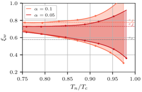
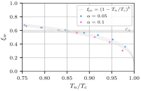
Figure 6: Left panel: Coloured regions indicate the forbidden regions of wall velocities. Coloured dashed lines indicate the Jouguet velocities for the two values of $\alpha$ (see Eq. (25)) while the dashed grey line labels the speed of sound. At high temperatures, Hydrodynamic obstruction limits the velocities of both detonation and deflagration solutions. At lower temperatures detonations are realised above the Jouguet velocity as expected, however, we find the obstruction limiting the maximal velocity of hybrids persists resulting in a range of hydrodynamical solutions that are not realised. High-temperature part of the limit on detonations relies on extrapolation and should be treated as a qualitative trend. Right panel: Our data for the maximal wall velocity on the deflagration/hybrid branch as a function of the nucleation temperature $T_{n}$ together with the fit from Eq. (26) (solid line) and its variation within $3\sigma$ of the best-fit parameters (dashed lines).

Fig. 6 shows the maximal wall velocity reached by the deflagration/hybrid solutions as a function of the nucleation temperature for different transition strengths. Given that in this limit of relatively large strength the result for hybrids does not depend significantly on $\alpha$ we found a simple fit

$$\xi_{w}^{max}=\left(1-\frac{T_{n}}{T_{c}}\right)^{k}\quad\textrm{with}\quad k=0.2768\pm 0.0055,$$ (26)

which can be used as a rough approximation for the upper bound for wall velocities. It has a similar origin as the relation proposed in Konstandin:2010dm , but is augmented with additional suppression that we observed for low temperatures, described by the power $k$.

4 Summary

We investigate the fluid solutions realised in the presence of growing bubbles in cosmological first order phase transitions. We use numerical lattice simulations using spherical symmetry of the system and compare results to the well known analytical solutions.

We found good agreement between the analytical profiles and our numerical results whenever the latter exist. Our key result, however, is that the hydrodynamical obstruction preventing the realisation of fast hybrids is very generic. In fact, we always find some solutions to be excluded and the gap in solutions becomes wider as the temperature at which bubbles nucleate predicted by the potential is closer to the critical temperature at which the minima in the potential are degenerate. In extreme cases where the temperatures are very close, no hybrid solutions are realised and as the friction drops the allowed solutions jump from subsonic deflagrations straight to detonations. The mechanism behind the obstruction is well understood in the case of deflagrations where the temperature profiles in the gap that are not realised would simply heat the plasma above the critical temperature and reverse the transition. In the case of hybrids the mechanism is more complicated and even solutions that do not reheat to such dangerous levels are not realised.

While the effect is yet to be confirmed directly in particular models we expect it to be general. Our calculations were performed for a simple toy potential, however, we express them in terms of general characteristics shared by all models predicting a first order transition. The existence of the velocity gap will have a crucial impact on predictions of models realising electroweak baryogenesis. This is due to the fact that the fastest walls that did not accelerate enough to become detonations are the ones most likely to be affected and the effect would persist even in low temperatures. Such solutions were recently shown to predict the largest baryon yields. Thus our results are likely to exclude parts of the parameter space of models most promising for electroweak baryogenesis and impact their viability as solutions to the problem of baryon asymmetry.

Acknowledgements

The authors would like to thank José Miguel No for fruitful discussions. This work was supported by the Polish National Agency for Academic Exchange within Polish Returns Programme under agreement PPN/PPO/2020/1/00013/U/00001 and the Polish National Science Center grant 2018/31/D/ST2/02048. T.K. was supported by grant 2019/32/C/ST2/00248 from the Polish National Science Centre. During the completion of this work, T.K. was supported by grant 2019/33/B/ST9/01564 from the Polish National Science Centre. T.K. acknowledges the hospitality of Rudolf Peierls Centre for Theoretical Physics at Oxford University, where parts of this work have been done.

Appendix A Discretization of the equations of motion

In order to obtain a numerical approximation of solutions of eqs. (9) and (11) we use the finite elements method, both in time and space.

To discretise in space we used the discontinuous Galerkin method. Our elements are just intervals of length $\delta r$ in the computational domain $[0,R]$. We used values of $R$ large enough to guarantee that the wall of the bubble is far from $r=R$ during the whole simulation, thus the choice of the boundary condition at this point does not influence the results.

Wave equation (9) describing the evolution of the scalar field is treated with a mixed scheme, i.e. we introduced auxiliary variable $\psi=\partial_{r}\phi$ which is interpolated using discontinuous piece-wise linear interpolation functions. Using the generalised trapezoid rule as numerical quadrature we obtained a second order scheme which is a generalization of the central finite difference scheme of the second order in Cartesian coordinates.

In the center of the bubble ($r=0$) we assumed the Neumann boundary condition for field $\phi$ which in the mixed formulation is just $\left.\psi\right|_{r=0}=0$. At the far edge of the computational lattice ($r=R$) we assumed the Dirichlet boundary condition setting the field value to the location of the false minimum.

In order to discretize the equation of motion of the field in time we used the discontinuous Galerkin method Tang:2012 ; Gagarina:2013 ; Zhao:2014 ; Campos:2014 ; Zhao:2014 ; Oberblobaum:2014 ; Gagarina:2016 ; Muehlebach:2016 ; Ober-Blobaum:2016 . The discontinuous piece-wise linear interpolation functions for $\phi$ and right-discontinuous linear interpolation for time derivative $\dot{\phi}$ result in a scheme mimicking the well-known position version of Strömer-Verlet scheme.

Deriving a numerical scheme for equations describing the evolution of plasma is somewhat more involved. We base our method on algebraic flux-corrected transport (FCT) proposed in Kuzmin:2002 ; Kuzmin:2003 ; Moller:2013 ; Kuzmin:2021 . Since the fluxes in eq. (11) are determined in terms of both conserved and so-called primitive variables $v$, $T$ (and derived from them $p$) one has to determine primitive ones from $\phi$, $\tau$ and $Z$ which are evolved in the code. In order to do so we combine (1) and (2) to find

$$\tau+p(\phi,T)-\frac{1}{2}\left(w(\phi,T)+\sqrt{w(\phi,T)^{2}+4Z^{2}}\right)=0$$ (27)

which we solve using the Raphson-Newton method to find the value of the temperature $T$. Then, $w$ and $p$ can be directly computed and the velocity $v$ can be simply computed by inverting the definition of $Z$.

In order to derive the high-order (in our case second order) scheme for FCT procedure we used the local discontinuous Galerkin method with piece-wise constant interpolation functions for conserved quantities $Z,\tau$, thus our scheme is similar to a finite volume method. To discretize the high-order scheme in time we use the midpoint method which can be derived as the discontinuous Galerkin method in time Tang:2012 ; Gagarina:2013 ; Zhao:2014 ; Campos:2014 ; Zhao:2014 ; Oberblobaum:2014 ; Gagarina:2016 ; Muehlebach:2016 ; Ober-Blobaum:2016 .

Our low-order scheme is obtained by the algebraic up-winding of the high-order scheme as described in Kuzmin:2002 ; Kuzmin:2003 ; Moller:2013 ; Kuzmin:2021 . The result is a scheme similar to the well-known Godunov scheme. To integrate the low-order scheme in time we used the backward Euler method since the forward Euler method turned out to be unstable for certain cases in the neighbourhood of center of the bubble $r=0$ and we exchanged the speed of the simulations in favour of the robustness of results. The sacrifice is not very severe, since up-winded advection matrix is band-limited with non-zero terms above diagonal only for nodes with negative velocity $v$ of plasma flow, so the implicit scheme can be efficiently implemented using Thomas’ algorithm.

The problem that we wanted to solve turned out to be demanding and we had to develop a new limiting procedure that will work properly during the whole simulation. Our attempt is based on well-known Zalesak’s limiter Zalesak:1979 in its peak-preserving version Zalesak:2012 corrected by the idea inspired by Kunhardt:1987 to restrict distances from which the conserved quantity values should be considered. The main observation is that the time step $\delta t$ used to integrate in time equations needs to satisfy the Courant-Friedrichs-Lewy condition, i.e.

$$\delta t\leq C\min{\left(\frac{\delta r}{|v|}\right)},$$ (28)

where $C$ is the so-called Courant number which depends on the used discretization scheme and $|v|$ is the maximal speed of propagation. For explicit time integration typically $C\lesssim 1$, thus the distance from which conserved quantity can be transported in a time step to a node which is bounded by the product $\delta t|v|$ must be smaller than the lattice spacing $\delta r$. As a result, it is more consistent to use in the limiter the values of conserved quantity in a distance of $\delta t|v|$ only, and not the values from the next node. Even though we conservatively assumed that the maximal speed is the speed of light, this correction significantly improved the robustness of our scheme.

Finally, the right-hand side of equations (9) and (11) can be consistently discretized using the Galerkin method with interpolation functions introduced above. Even though, interpolation functions in time were chosen in such a way to obtain explicit schemes even when $\eta$ dependent terms are included, the implicit term for $\dot{\phi}$ arises from the right-hand side of (9). Fortunately, the dependence on $\dot{\phi}$ and the implicit equation can be solved exactly.

Appendix B General results for polynomial potentials

The simplest polynomial renormalizable potential takes the form

$$V(\phi)=m^{2}\phi^{2}-a\phi^{3}+\lambda\phi^{4},$$ (29)

where $m^{2}$, $a$ and $\lambda$ may depend on the temperature. For such potential, there exists an accurate semi-analytical approximation of the critical actionAdams:1993zs ; Ellis:2020awk :

$$\frac{S_{3}}{T}=\frac{a}{T\lambda^{3/2}}\frac{8\pi\sqrt{\beta_{1}\delta+\beta_{2}\delta^{2}+\beta_{3}\delta^{3}}}{81(2-\delta)^{2}},$$ (30)

where $\delta$ = $\frac{8\lambda m^{2}}{a^{2}}$ and $\beta_{1}=8.2938$, $\beta_{2}=-5.5330$, $\beta_{3}=0.8180$. Therefore the nucleation rate for the potential (3) may be estimated as

$$\frac{\Gamma}{H^{4}}=\frac{T^{4}\exp{(-\frac{S_{3}}{T}})}{\rho_{r}+\rho_{V}}=\frac{\exp{(-\frac{8\pi\alpha(\frac{4\delta}{\lambda})^{3/2}(\beta_{1}+\beta_{2}\delta+\beta_{3}\delta^{2})}{243(\delta-2)^{2}})}}{\left(\frac{T_{0}^{2}}{1-\frac{\pi^{2}\alpha^{2}}{9\pi^{2}\gamma\lambda}}\delta\right)^{2}\left(\frac{1}{3M_{pl}^{2}}\right)^{2}\left(\frac{\pi^{2}g_{*}}{30}+(4\pi\alpha)^{4}\frac{(\sqrt{9-4\delta}+3)^{2}(\sqrt{9-4\delta}+3-2\delta)}{2\cdot 24^{4}\pi^{4}\lambda^{3}}\right)^{2}}.$$ (31)

This expression depends on the temperature only through dimensionless parameter $\delta$, which varies from $\delta=0$ at $T_{0}$ to $\delta=2$ at $T_{c}$. Using this significantly simplifies the calculations, as the value of $\delta$ for which $\frac{\Gamma}{H^{4}}=1$ can be easily translated into $T_{n}$.

References

- (1) V. A. Kuzmin, V. A. Rubakov, and M. E. Shaposhnikov, “On the Anomalous Electroweak Baryon Number Nonconservation in the Early Universe,” Phys. Lett. B, vol. 155, p. 36, 1985.
- (2) A. G. Cohen, D. B. Kaplan, and A. E. Nelson, “Progress in electroweak baryogenesis,” Ann. Rev. Nucl. Part. Sci., vol. 43, pp. 27–70, 1993.
- (3) V. A. Rubakov and M. E. Shaposhnikov, “Electroweak baryon number nonconservation in the early universe and in high-energy collisions,” Usp. Fiz. Nauk, vol. 166, pp. 493–537, 1996.
- (4) D. E. Morrissey and M. J. Ramsey-Musolf, “Electroweak baryogenesis,” New J. Phys., vol. 14, p. 125003, 2012.
- (5) C. Caprini et al., “Science with the space-based interferometer eLISA. II: Gravitational waves from cosmological phase transitions,” JCAP, vol. 04, p. 001, 2016.
- (6) C. Caprini et al., “Detecting gravitational waves from cosmological phase transitions with LISA: an update,” JCAP, vol. 03, p. 024, 2020.
- (7) Y. A. El-Neaj et al., “AEDGE: Atomic Experiment for Dark Matter and Gravity Exploration in Space,” EPJ Quant. Technol., vol. 7, p. 6, 2020.
- (8) L. Badurina, O. Buchmueller, J. Ellis, M. Lewicki, C. McCabe, and V. Vaskonen, “Prospective sensitivities of atom interferometers to gravitational waves and ultralight dark matter,” Phil. Trans. A. Math. Phys. Eng. Sci., vol. 380, no. 2216, p. 20210060, 2021.
- (9) J. M. Cline and K. Kainulainen, “Electroweak baryogenesis at high bubble wall velocities,” Phys. Rev. D, vol. 101, no. 6, p. 063525, 2020.
- (10) B. Laurent and J. M. Cline, “Fluid equations for fast-moving electroweak bubble walls,” Phys. Rev. D, vol. 102, no. 6, p. 063516, 2020.
- (11) J. M. Cline, A. Friedlander, D.-M. He, K. Kainulainen, B. Laurent, and D. Tucker-Smith, “Baryogenesis and gravity waves from a UV-completed electroweak phase transition,” Phys. Rev. D, vol. 103, no. 12, p. 123529, 2021.
- (12) G. C. Dorsch, S. J. Huber, and T. Konstandin, “On the wall velocity dependence of electroweak baryogenesis,” JCAP, vol. 08, p. 020, 2021.
- (13) J. M. Cline and B. Laurent, “Electroweak baryogenesis from light fermion sources: A critical study,” Phys. Rev. D, vol. 104, no. 8, p. 083507, 2021.
- (14) M. Lewicki, M. Merchand, and M. Zych, “Electroweak bubble wall expansion: gravitational waves and baryogenesis in Standard Model-like thermal plasma,” JHEP, vol. 02, p. 017, 2022.
- (15) G. C. Dorsch, S. J. Huber, and T. Konstandin, “A sonic boom in bubble wall friction,” JCAP, vol. 04, no. 04, p. 010, 2022.
- (16) B. Laurent and J. M. Cline, “First principles determination of bubble wall velocity,” Phys. Rev. D, vol. 106, no. 2, p. 023501, 2022.
- (17) J. Ellis, M. Lewicki, M. Merchand, J. M. No, and M. Zych, “The scalar singlet extension of the Standard Model: gravitational waves versus baryogenesis,” JHEP, vol. 01, p. 093, 2023.
- (18) J. M. No, “Large Gravitational Wave Background Signals in Electroweak Baryogenesis Scenarios,” Phys. Rev. D, vol. 84, p. 124025, 2011.
- (19) J. R. Espinosa, T. Konstandin, J. M. No, and G. Servant, “Energy Budget of Cosmological First-order Phase Transitions,” JCAP, vol. 06, p. 028, 2010.
- (20) D. Kuzmin and S. Turek, “Flux correction tools for finite elements,” Journal of Computational Physics, vol. 175, no. 2, pp. 525–558, 2002.
- (21) D. Kuzmin, M. Möller, and S. Turek, “Multidimensional fem-fct schemes for arbitrary time stepping,” International Journal for Numerical Methods in Fluids, vol. 42, no. 3, pp. 265–295, 2003.
- (22) M. Möller, “Algebraic flux correction for nonconforming finite element discretizations of scalar transport problems,” Computing, vol. 95, p. 425–448, may 2013.
- (23) D. Kuzmin, “A new perspective on flux and slope limiting in discontinuous galerkin methods for hyperbolic conservation laws,” Computer Methods in Applied Mechanics and Engineering, vol. 373, p. 113569, 2021.
- (24) S. T. Zalesak, “Fully multidimensional flux-corrected transport algorithms for fluids,” Journal of Computational Physics, vol. 31, no. 3, pp. 335–362, 1979.
- (25) J. Ignatius, K. Kajantie, H. Kurki-Suonio, and M. Laine, “The growth of bubbles in cosmological phase transitions,” Phys. Rev. D, vol. 49, pp. 3854–3868, 1994.
- (26) H. Kurki-Suonio and M. Laine, “On bubble growth and droplet decay in cosmological phase transitions,” Phys. Rev. D, vol. 54, pp. 7163–7171, 1996.
- (27) H. Kurki-Suonio, K. Jedamzik, and G. J. Mathews, “Stochastic isocurvature baryon fluctuations, baryon diffusion, and primordial nucleosynthesis,” Astrophys. J., vol. 479, pp. 31–39, 1997.
- (28) M. Hindmarsh, S. J. Huber, K. Rummukainen, and D. J. Weir, “Gravitational waves from the sound of a first order phase transition,” Phys. Rev. Lett., vol. 112, p. 041301, 2014.
- (29) M. Hindmarsh, S. J. Huber, K. Rummukainen, and D. J. Weir, “Numerical simulations of acoustically generated gravitational waves at a first order phase transition,” Phys. Rev. D, vol. 92, no. 12, p. 123009, 2015.
- (30) M. Kamionkowski and K. Freese, “Instability and subsequent evolution of electroweak bubbles,” Phys. Rev. Lett., vol. 69, pp. 2743–2746, 1992.
- (31) S. R. Coleman, “The Fate of the False Vacuum. 1. Semiclassical Theory,” Phys. Rev. D, vol. 15, pp. 2929–2936, 1977. [Erratum: Phys.Rev.D 16, 1248 (1977)].
- (32) C. G. Callan, Jr. and S. R. Coleman, “The Fate of the False Vacuum. 2. First Quantum Corrections,” Phys. Rev. D, vol. 16, pp. 1762–1768, 1977.
- (33) A. D. Linde, “Fate of the False Vacuum at Finite Temperature: Theory and Applications,” Phys. Lett. B, vol. 100, pp. 37–40, 1981.
- (34) A. D. Linde, “Decay of the False Vacuum at Finite Temperature,” Nucl. Phys. B, vol. 216, p. 421, 1983. [Erratum: Nucl.Phys.B 223, 544 (1983)].
- (35) J. Ellis, M. Lewicki, and J. M. No, “On the Maximal Strength of a First-Order Electroweak Phase Transition and its Gravitational Wave Signal,” JCAP, vol. 04, p. 003, 2019.
- (36) M. Hindmarsh, S. J. Huber, K. Rummukainen, and D. J. Weir, “Shape of the acoustic gravitational wave power spectrum from a first order phase transition,” Phys. Rev. D, vol. 96, no. 10, p. 103520, 2017. [Erratum: Phys.Rev.D 101, 089902 (2020)].
- (37) P. Auclair et al., “Cosmology with the Laser Interferometer Space Antenna,” 4 2022.
- (38) M. Hindmarsh and M. Hijazi, “Gravitational waves from first order cosmological phase transitions in the Sound Shell Model,” JCAP, vol. 12, p. 062, 2019.
- (39) J. Ellis, M. Lewicki, and J. M. No, “Gravitational waves from first-order cosmological phase transitions: lifetime of the sound wave source,” JCAP, vol. 07, p. 050, 2020.
- (40) P. J. Steinhardt, “Relativistic Detonation Waves and Bubble Growth in False Vacuum Decay,” Phys. Rev. D, vol. 25, p. 2074, 1982.
- (41) M. Lewicki, V. Vaskonen, and H. Veermäe, “Bubble dynamics in fluids with N-body simulations,” Phys. Rev. D, vol. 106, no. 10, p. 103501, 2022.
- (42) T. Konstandin and J. M. No, “Hydrodynamic obstruction to bubble expansion,” JCAP, vol. 02, p. 008, 2011.
- (43) W. Tang and Y. Sun, “Time finite element methods: A unified framework for numerical discretizations of odes,” Applied Mathematics and Computation, vol. 219, no. 4, pp. 2158–2179, 2012.
- (44) E. Gagarina, J. van der Vegt, V. Ambati, and O. Bokhove, Variational space-time (dis)continuous Galerkin method for nonlinear free surface waves. No. 2008 in Memorandum, University of Twente, Department of Applied Mathematics, May 2013.
- (45) S. Zhao and G. W. Wei, “A unified discontinuous galerkin framework for time integration,” Mathematical Methods in the Applied Sciences, vol. 37, no. 7, pp. 1042–1071, 2014.
- (46) C. M. Campos, High Order Variational Integrators: A Polynomial Approach, pp. 249–258. Cham: Springer International Publishing, 2014.
- (47) S. Ober-Blöbaum and N. Saake, “Construction and analysis of higher order galerkin variational integrators,” 2014.
- (48) E. Gagarina, V. Ambati, S. Nurijanyan, J. van der Vegt, and O. Bokhove, “On variational and symplectic time integrators for hamiltonian systems,” Journal of Computational Physics, vol. 306, pp. 370–389, 2016.
- (49) M. Muehlebach, T. Heimsch, and C. Glocker, “Variational integrators – a continuous time approach,” 2016.
- (50) S. Ober-Blöbaum, “Galerkin variational integrators and modified symplectic Runge–Kutta methods,” IMA Journal of Numerical Analysis, vol. 37, pp. 375–406, 02 2016.
- (51) S. T. Zalesak, The Design of Flux-Corrected Transport (FCT) Algorithms for Structured Grids, pp. 23–65. Dordrecht: Springer Netherlands, 2012.
- (52) E. Kunhardt and C. Wu, “Towards a more accurate flux corrected transport algorithm,” Journal of Computational Physics, vol. 68, no. 1, pp. 127–150, 1987.
- (53) F. C. Adams, “General solutions for tunneling of scalar fields with quartic potentials,” Phys. Rev. D, vol. 48, pp. 2800–2805, 1993.