Contrastive-Signal-Dependent Plasticity: Forward-Forward Learning of
Spiking Neural Systems

Abstract

We develop a neuro-mimetic architecture, composed of spiking neuronal units, where individual layers of neurons operate in parallel and adapt their synaptic efficacies without the use of feedback pathways. Specifically, we propose an event-based generalization of forward-forward learning, which we call contrastive-signal-dependent plasticity (CSDP), for a spiking neural system that iteratively processes sensory input over a stimulus window. The dynamics that underwrite this recurrent circuit entail computing the membrane potential of each processing element, in each layer, as a function of local bottom-up, top-down, and lateral signals, facilitating a dynamic, layer-wise parallel form of neural computation. Unlike other models, such as spiking predictive coding, which rely on feedback synapses to adjust neural electrical activity, our model operates purely online and forward in time, offering a promising way to learn distributed representations of sensory data patterns, with and without labeled context information. Notably, our experimental results on several pattern datasets demonstrate that the CSDP process works well for training a dynamic recurrent spiking network capable of both classification and reconstruction.

Keywords Forward learning  $\cdot$ Spiking neural networks  $\cdot$ Brain-inspired learning  $\cdot$ Credit assignment
 $\cdot$ Neuromorphic computing  $\cdot$ Neuro-mimetic systems  $\cdot$ Synaptic plasticity  $\cdot$ Self-supervised learning

1 Introduction

The notion of “mortal computation” [26] challenges one of the foundational principles upon which general purpose computers have been built. Specifically, computation, as it is conducted today, is driven by the strong separation of software from hardware, i.e., this means that the knowledge contained within a program written in the software is “immortal”, allowing it to be copied to different physical copies of the hardware itself. Machine learning models and algorithms, which can be viewed as programs that adjust themselves in accordance with data, also rely upon this separation. Mortal computation, in contrast, means that once the hardware medium fails or “dies”, the knowledge encoded within it will also “die” or disappear, much akin to what would happen to the knowledge acquired by a biological organism when it is no longer able to maintain homeostasis. Despite the seeming disadvantage that comes with tightly bounding the software’s fate with that of the hardware it is implemented within, abandoning the immortal nature of computation brings with it the important promise of substantial savings in energy usage as well as a reduction in the cost of creating the hardware needed to execute the required computations. Working towards mortal computation addresses some of the concerns and questions that have recently emerged in artificial intelligence (AI) research [1, 5, 86, 80, 70]: how may we design intelligent systems that do not escalate computational and carbon costs? In essence, there is a strong motivation to move away from Red AI, which is driven by the dominance of immortal computation, towards Green AI [80], which mortal computation would naturally facilitate.

As was further argued in [63], moving towards mortal computation would also likely entail challenging an important separation made in deep learning – the separation between inference and credit assignment. Specifically, deep neural networks, including the more recent neural transformers [12, 17, 6] that drive large language models (typically pre-trained on gigantic text databases), are fit to training datasets in such a way that learning or credit assignment, carried out via the backpropagation of errors (backprop) algorithm [75], is treated as a separate computation distinct from the mechanisms in which information is propagated through the network itself. In contrast, an adaptive system that could take advantage of mortal computing will most likely need to engage in intertwined inference-and-learning [69, 68, 64, 62]. It follows from such a view that learning and inference in the brain are not likely two completely distinct, separate processes but rather complementary ones that depend on and support one another, the formulations of which are motivated and integrated with the properties of the underlying neural circuitry (and the hardware that instantiates it), lending itself to more energy-efficient calculations, e.g., in-memory operations [71, 90]. Neural systems, in this context, would adapt to external sensory information based on the properties of the hardware that they run on, governed by homeostatic-like constraints. As a result, it would be beneficial for research in brain-inspired credit assignment to look to frameworks that embody intertwined inference-and-learning as well as facilitate implementation on energy-efficient hardware platforms; important candidate frameworks include predictive processing/coding [73, 19, 83, 62, 77], contrastive Hebbian learning [51, 56, 79], and forward-only learning [34, 26, 63, 33], each with their own strengths and weaknesses. This direction could prove invaluable for AI research, providing not only another important link between cognitive science, computational neuroscience, and machine learning, but also a critical means of running neural systems composed of trillions of synapses (as in the brain), while only consuming a few watts of energy.

Among the potential forms of hardware that could embody mortal computation and intertwined inference-and-learning, e.g., memristors [29, 87], liquid crystal spatial light modulators [7, 14], Field Programmable Gate Arrays (FPGAs) [38, 55], neuromorphic chips [20, 74] have emerged as promising candidates. Neuromorphic platforms offer an incredibly efficient, low-energy means of conducting numerical calculations, facilitating resource-constrained edge computation [37, 10]. Spiking neural networks (SNNs), sometimes branded as the third generation of neural networks [43, 45, 44, 15, 16], are a particular type of brain-inspired adaptive system and are naturally suited for implementation in neuromorophic hardware. Properly exploiting the design and properties of such chips enables the crafting of model and algorithmic designs that embody mortal computation. However, developing effective, stable processes for conducting credit assignment in SNNs remains a challenge, particularly given that the underlying process of synaptic adjustment will need to rely on local information provided by discretely spiking neuronal units. Furthermore, important qualities that should characterize the computations underwriting the inference and learning of spiking systems should include: 1) no requirement for differentiability in the spike-based communication (backprop through time as applied to SNNs requires differentiability and thus the careful design of surrogate functions [49, 91]), 2) no forward-locking [31] in the information propagation (a layer of neurons can compute their activity values without waiting on other layers to update their own), 3) no backward-locking[31] in the synaptic update phase (adjustments to synapses for one layer of neurons can be executed in parallel with other layers across time – updates are local in both space and time), and 4) no feedback synaptic pathways are fundamentally required to calculate synaptic change (promising biological frameworks such as predictive coding require synaptic pathways to carry out the requisite message passing [73, 19, 2, 72, 59, 54]).

In this work, we satisfy the above criterion by developing a novel formulation of forward-only-based credit assignment [34], specifically that of forward-forward (FF) [26] and predictive forward-forward (PFF) [63] learning, for the case of systems that center around spike-based communication. Our core contributions in this study include:

1. the design of a recurrent spiking neural network that fundamentally exhibits layer-wise parallelism, driven by a top-down, bottom-up, and lateral set of pressures that do not require feedback synaptic pathways – this means that our (intertwined) learning and inference process resolves the forward and update locking problems that characterize backprop-based credit assignment,

2. the proposal of contrastive-signal-dependent plasticity (CSDP) for locally adapting the synapses of spiking neural systems in an online, dynamic fashion, potentially serving as a process that could complement spike-timing dependent plasticity (STDP) [4],

3. the development of a simple and fast mechanism for learning a spike-based classifier without resorting to the expensive energy-based classification scheme that characterizes FF and PFF-based systems, and

4. a quantitative evaluation of the generalization ability of our spiking system learned with CSDP.

2 Learning Spiking Networks with Event-Driven Forward-Forward Adjustment

Notation. We use $\odot$ to indicate the Hadamard product (or element-wise multiplication) and $\cdot$ to denote a matrix/vector multiplication. $(\mathbf{v})^{\mathsf{T}}$ is the transpose of $\mathbf{v}$. Matrices/vectors are depicted in bold font, e.g., matrix $\mathbf{M}$ or vector $\mathbf{v}$ (scalars shown in italic). $\mathbf{z}_{j}$ will refer to extracting $j$th scalar from vector $\mathbf{z}$. Finally, $||\mathbf{v}||_{2}$ denotes the Euclidean norm of vector $\mathbf{v}$. A sensory input pattern has shape $\mathbf{x}\in\mathcal{R}^{J_{0}\times 1}$ ($J_{0}$ is the number of input features, e.g., pixels), a label vector has shape $\mathbf{y}\in\mathcal{R}^{C\times 1}$ (where $C$ is the number of classes), and any layer inside a neural system has shape $\mathbf{z}^{\ell}\in\mathcal{R}^{J_{\ell}\times 1}$; note that $J_{\ell}$ is the number of neurons in layer $\ell$.

2.1 The Recurrent Spiking Neural Circuit Dynamics

The neural system that we will design and study is composed of recurrent layers that operate in parallel with each other, i.e., at time $t$, each layer $\ell$, made up of $J_{\ell}$ neuronal cells, will take in as input the previous (spike) signals emitted (at time $t-1$) from the neurons immediately below (from layer $\ell-1$) as well as from those immediately above (from layer $\ell+1$). Optionally, each layer receives a projection of a top-down “attentional” context-mediating (spike) signals, which will be in encouraging neural units to form representations that encode any available discriminative

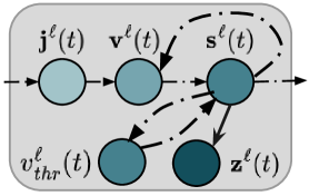
Figure 1: Our LIF cell group and their modeled internal compartments.

information, such as that found within existing labels/annotations. Finally, the neurons in each of these layers will be laterally connected to each other, where the synapses that relate them will enforce a form of dynamic inhibition, i.e., neurons that more strongly active will suppress the activities of others, resulting in an emergent form of $K$ winners-take-all competition, where $K$ changes with time.

Formally, the full model, composed of $L$ layers of neural processing elements (NPEs), is parameterized by the construct $\Theta=\{\mathbf{W}^{1},\mathbf{V}^{1},\mathbf{M}^{1},\mathbf{B}^{1},...,\mathbf{W}^{\ell},\mathbf{V}^{\ell},\mathbf{M}^{\ell},\mathbf{B}^{\ell},...\mathbf{W}^{L},\mathbf{M}^{L},\mathbf{B}^{L}\}$. As described before, each layer’s stateful activation is driven by messages passed along bottom-up synapses (inside matrix $\mathbf{W}^{\ell}\in[-1,1]^{J_{\ell}\times J_{\ell-1}}$), top-down mediating synapses (inside matrix $\mathbf{V}^{\ell}\in[-1,1]^{J_{\ell}\times J_{\ell+1}}$), lateral inhibition synapses (inside matrix $\mathbf{M}^{\ell}\in[0,1]^{J_{\ell}\times J_{\ell}}$), and optional context-mediating synapses (inside matrix $\mathbf{B}^{\ell}\in[-1,1]^{J_{\ell}\times C}$). In this work, we further constrain all of the constituent matrices to contain values that are bounded between $-1$ and $1$, except for $\mathbf{M}^{\ell}$, which itself is restricted to positive values in the range of $[0,1]$. The dynamics of any NPE/cell in layer $\ell$ of our spiking system follow that of a leaky integrator; specifically, the full dynamics of a layer of spiking NPEs are calculated in terms of electrical current:

$$\mathbf{j}^{\ell}(t)=\begin{cases}\mathbf{W}^{\ell}\cdot\mathbf{s}^{\ell-1}(t)+\mathbf{V}^{\ell}\cdot\mathbf{s}^{\ell+1}(t)-(\mathbf{M}^{\ell}\odot(1-\mathbf{I}^{\ell}))\cdot\mathbf{s}^{\ell}(t)&\text{// Unsupervised form}\\ \mathbf{W}^{\ell}\cdot\mathbf{s}^{\ell-1}(t)+\mathbf{V}^{\ell}\cdot\mathbf{s}^{\ell+1}(t)-(\mathbf{M}^{\ell}\odot(1-\mathbf{I}^{\ell}))\cdot\mathbf{s}^{\ell}(t)+\mathbf{B}^{\ell}\cdot\mathbf{s}_{y}(t)&\text{// Context-driven form},\end{cases}$$ (1)

as well as membrane voltage potential and an action potential (or spike) emission function:

$$\mathbf{v}^{\ell}(t+\Delta t) =\mathbf{v}^{\ell}(t)+\frac{\Delta t}{\tau_{m}}\Big{(}-\mathbf{v}^{\ell}(t)+R_{m}\mathbf{j}^{\ell}(t)\Big{)}$$ (2)

$$\mathbf{s}^{\ell}(t) =\mathbf{v}^{\ell}(t+\Delta t)>v^{\ell}_{thr},\;\mbox{and, }\;\mathbf{v}^{\ell}(t)=\mathbf{v}^{\ell}(t+\Delta t)\odot(1-\mathbf{s}^{\ell}(t))$$ (3)

$$v^{\ell}_{thr} =v^{\ell}_{thr}+\lambda_{v}\Big{(}(\sum^{J_{\ell}}_{j=1}\mathbf{s}^{\ell}(t)_{j})-1\Big{)}$$ (4)

where, for a given layer $\ell$ at time $t$, $\mathbf{j}^{\ell}(t)$ is the vector containing the electrical current input to each cell in the layer, $\mathbf{v}^{\ell}(t)$ is the vector containing the current membrane potential (voltage) values for each cell, and $\mathbf{s}^{\ell}(t)$ is the vector containing each cell’s binary spike output. $R_{m}$ is the resistance constant, (deci)Ohms, for layer $\ell$, $\Delta t$ is the integration time constant on the order of milliseconds (ms), and $\tau_{m}$ is the membrane time constant (in ms). In Equation 3, we depolarize the membrane voltage back to a resting potential of $0$ (deci)volts through binary gating and do not consider modeling a refractory period; we omit both relative and absolute refractory periods for simplicity. Notice in Equation 4, we simulate a simple adaptive non-negative threshold $v^{\ell}_{thr}\in[0,\infty)$ which, at each time step $t$, either adds or subtracts a small value – scaled by $\lambda_{v}$, typically set to a number such as $0.001$ – to a current threshold value based on how many spikes were recorded at time step $t$ for layer $\ell$. Finally, $\mathbf{s}^{0}(t)$ is the binary spike representation of the sensory input $\mathbf{x}$ at time $t$ and is created by sampling the normalized pixel values of $\mathbf{x}$ (each dimension of $\mathbf{x}$ is divided by the maximum pixel value $255$), treating each dimension as Bernoulli probability. $\mathbf{s}_{y}(t)$ is the contextual spike train associated with $\mathbf{x}$, i.e., in this study, if a label is available, then $\mathbf{s}_{y}(t)=\mathbf{y}$ (it is clamped to the label during training), otherwise $\mathbf{s}_{y}(t)=\emptyset$.

A useful property of the recurrent spiking system above is that it is layer-wise parallelizable and thus naturally not forward-locked [31]; this means that the spike activities at any layer can be computed in parallel of the others. Furthermore, as we will see later, the system is not update/backward-locked or, in other words, the synaptic updates for any layer can be computed in parallel of the others. This stands in contrast to many (deep) SNN designs today, with some exceptions [72, 59, 54], given that many are typically feedforward, where each layer of spiking neurons depends on the spike activities of the layer that comes before them resulting in an inherently forward-locked computation. Our spiking model ensures this important form of model-level parallelism by only enforcing leaky integrator spike activities to only depend upon recently computed activities (those of simulation step $t-1$).

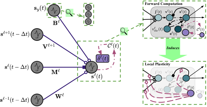
Figure 2: Depicted is the neural computation underlying our recurrent spiking network and its synaptic adjustment induced via contrastive-signal-dependent plasticity. To facilitate a contrastive form of learning, we posit the existence of another biochemical compartment $\mathbf{\delta}^{\ell}(t)$ in our leaky integrator cell. Once electrical current $\mathbf{j}^{\ell}(t)$ has been injected into the cells, triggering an update to their membrane potentials $\mathbf{v}^{\ell}(t)$, possibly leading to the emission of action potentials $\mathbf{s}^{\ell}(t)$, their glutamate traces contribute to a goodness modulator $\mathcal{C}^{\ell}(t)$ which then deposits a local synaptic adjustment signal to each cell’s $\delta^{\ell}_{i}(t)$ compartment.

Online Plasticity Dynamics. One key building block to our event-driven contrastive learning process is the trace variable. Specifically, in our recurrent spiking system above, we incorporate an additional compartment into each neural layer that is responsible for maintaining what is called an activity variable trace (or activation trace). Formally, this means that for each layer, a variable trace is dynamically updated as follows:

$$\mathbf{z}^{\ell}(t)=\mathbf{s}^{\ell}(t)-\frac{\Delta t}{\tau_{tr}}\mathbf{z}^{\ell}(t)\odot\big{(}1-\mathbf{s}^{\ell}(t)\big{)}$$ (5)

where, in this work, the trace time constant was set to $\tau_{tr}=300$ ms. Importantly, an activation trace smooths out the sparse spike trains generated by the spiking model while still being biologically-plausible. Notably, a trace offers a dynamic rate-coded equivalent value that, in our neuronal layer model, is maintained within the actual neuronal cells likely in the form of the concentration of internal calcium ions [58], i.e., a variable trace could correspond to the glutamate bound to synaptic receptors. Desirably, this will allow our local adaptation rule to take place using (filtered) spike information, bringing it closer to STDP-like learning, rather than being used directly on the voltage or electrical current values, like in other related efforts [33].

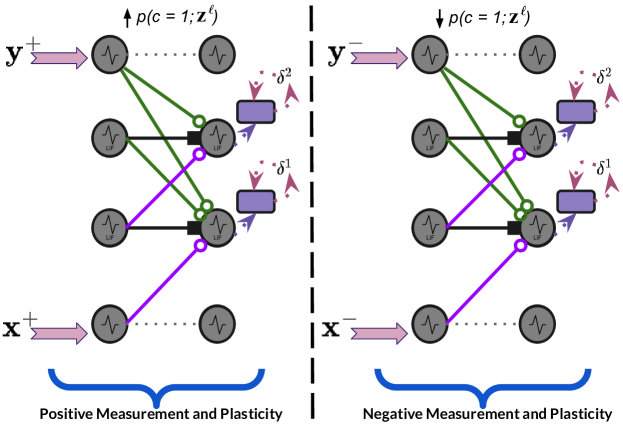
Figure 3: Shown are the two parallel modes of plasticity that our recurrent spiking circuit undergoes – a positive measurement mode where a sensory input and its corresponding (if available) context are used to drive inference and plasticity (to raise probabilities assigned to a sensory pattern), and a negative measurement mode where a negative / out-of-distribution sample and its corresponding negative context are used to drive the same underlying neural calculations (to lower assigned probabilities).

Given the activation trace above, we can now formulate the objective that each layer of our spiking system will try to optimize at each step of simulated time. Specifically, in our learning process, contrastive-signal-dependent plasticity (CSDP), we propose adjusting the synaptic strengths in the recurrent spiking model above by integrating the ‘goodness principle’ inherent to forward-forward learning [26, 63] into the dynamics of spiking neurons – this concretely means that any layer of NPEs will work to raise the probability they (collectively) assign to incoming pre-synaptic messages that they receive if the sensory input is comes from the environment, i.e., it is ‘positive’, and strive to lower the probability they assign if the input is ‘fake’ or non-sensical, i.e., it is ‘negative’ (see Figure 3). As a result, the (local) cost functional takes the following form:

$$\mathcal{C}(\mathbf{z}^{\ell}(t),y_{type})=-\Big{(}\overbrace{y_{type}\log p(y_{type}=1;\mathbf{z}^{\ell})}^{\text{Positive Term}}+\overbrace{(1-y^{\ell}_{type})\log p(y_{type}=0;\mathbf{z}^{\ell})}^{\text{Negative Term}}\Big{)},$$ (6)

where the probability $p(y_{type}=1;\mathbf{z}^{\ell})$ is further defined as:

$$p(y_{type}=1;\mathbf{z}^{\ell})=\frac{1}{1+\exp\big{(}-(\sum^{J_{\ell}}_{j=1}(\mathbf{z}^{\ell}_{j}(t))^{2}-\theta_{z})\big{)}}.$$ (7)

$y_{type}\in\{0,1\}$ is an integer that denotes what ‘type’ of sensory input incoming (pre-synaptic) activity to layer $\ell$ originates from, i.e., $1$ indicates that it originates from positive (in-distribution) sensory input while $0$ indicates that it comes from negative (out-of-distribution) sensory input. $\theta_{z}$ is a threshold for comparing the square of the trace activity values against, set to $\theta_{z}=6.5$ in this paper. Given the local cost functional defined in Equation 6, we defined the update to each synaptic matrix feeding into any one layer of the neuronal system in accordance to the following Hebbian-like adjustment scheme:

$$\delta^{\ell}(t) =2\frac{\partial\mathcal{C}(\mathbf{z}^{\ell}(t),y_{type})}{\partial\sum^{J_{\ell}}_{j}(\mathbf{z}^{\ell}_{j}(t))^{2}}$$ (8)

$$\Delta\mathbf{W}^{\ell} =\big{(}R_{m}\delta^{\ell}(t)\cdot\big{(}\mathbf{s}^{\ell-1}(t-1)\big{)}^{T}\big{)}+\lambda_{d}\big{(}\mathbf{s}^{\ell}(t)\cdot(1-\mathbf{s}^{\ell-1}(t))^{T}\big{)}$$ (9)

$$\Delta\mathbf{V}^{\ell} =\big{(}R_{m}\delta^{\ell}(t)\cdot\big{(}\mathbf{s}^{\ell+1}(t-1)\big{)}^{T}\big{)}+\lambda_{d}\big{(}\mathbf{s}^{\ell}(t)\cdot(1-\mathbf{s}^{\ell+1}(t))^{T}\big{)}$$ (10)

$$\Delta\mathbf{M}^{\ell} =\big{(}R_{m}\delta^{\ell}(t)\cdot\big{(}\mathbf{s}^{\ell}(t-1)\big{)}^{T}\big{)}+\lambda_{d}\big{(}\mathbf{s}^{\ell}(t)\cdot(1-\mathbf{s}^{\ell}(t))^{T}\big{)}$$ (11)

$$\Delta\mathbf{B}^{\ell} =\big{(}R_{m}\delta^{\ell}(t)\cdot\big{(}\mathbf{s}_{y}(t-1)\big{)}^{T}+\lambda_{d}\big{(}\mathbf{s}^{\ell}(t)\big{)}\cdot(1-\mathbf{s}^{y}(t))^{T}\big{)}$$ (12)

where $\lambda_{d}=0.00005$ is the synaptic decay factor. Notice that the update to each of the three or four key synaptic matrices which characterize the computation of layer $\ell$ depends on the easily computed partial derivative $\delta^{\ell}(t)$ of the local contrastive function $\mathcal{C}(\mathbf{z}^{\ell}(t),y_{type})$. We postulate that, biologically, $\delta^{\ell}(t)$ (scaled by the resistance $R_{m}$) would be implemented either in the form of a (neurotransmitter) chemical signal or alternatively as a separate population of neural units that encode this signal (much akin to the error neurons that characterize predictive processing [9]). If one adopts the neurotransmitter point-of-view, then the above synaptic plasticity equations could be likened to multi-factor Hebbian rules where the modulator/scaling term is deposited from a locally embedded compartment that emulates a contrastive functional $\mathcal{C}(\mathbf{z}^{\ell}(t),y_{type})$, as opposed to the typically used temporal difference error or reward value found in three-factor (neuromodulated) Hebbian/STDP update schemes. See Figure 2 for a visual depiction of the mechanics that underpin this form of plasticity. We illustrate the two ‘modes’ of plasticity that our system undergoes in Figure 3; specifically, if an in-distribution sensory pattern (and possibly its corresponding context) is fed in, then each layer in the system tries to increase the probability it assigns to the pattern whereas, for a non-sensical (out-of-distribution) pattern, each layer tries to decrease this probability.

A CSDP-SNN as a Spiking Generative Model. To incorporate the reconstruction/generative potential of the predictive forward-forward (PFF) adaptation process [63], we introduce one more set of matrices which contain the generative synapses – this means that we extend our model parameters to $\Theta\bigcup\Theta_{g}$ where $\Theta_{g}=\{\mathbf{G}^{\ell}\}^{L}_{\ell=1}$. Desirably, each synaptic matrix $\mathbf{G}^{\ell}$ is directly wired to each layer $\ell$, forming a local prediction of the activity of $\mathbf{s}^{\ell}(t)$ in the following manner:

$$\mathbf{v}^{\ell}_{\mu}(t+\Delta t) =\mathbf{v}^{\ell}_{\mu}(t)+\frac{\Delta t}{\tau_{m}}\Big{(}-\mathbf{v}^{\ell}_{\mu}(t)+R_{m}(\mathbf{G}^{\ell+1}\cdot\mathbf{s}^{\ell+1}(t))\Big{)}$$ (13)

$$\mathbf{s}^{\ell}_{\mu}(t) =\mathbf{v}^{\ell}_{\mu}(t+\Delta t)>v^{\ell}_{thr,\mu},\quad\mathbf{v}^{\ell}_{\mu}(t)=\mathbf{v}^{\ell}_{\mu}(t+\Delta t)\odot(1-\mathbf{s}^{\ell}_{\mu}(t))$$ (14)

$$\mathbf{e}^{\ell}(t) =\mathbf{s}^{\ell}_{\mu}(t)-\mathbf{s}^{\ell}(t)$$ (15)

$$v^{\ell}_{thr,\mu} =v^{\ell}_{thr,\mu}+\lambda_{v}\Big{(}(\sum^{J_{\ell}}_{j=1}\mathbf{s}^{\ell}_{\mu,j}(t))-1\Big{)}$$ (16)

where we observe that error mismatch units $\mathbf{e}^{\ell}(t)$ have been introduced that specialize in tracking the disparity between prediction spikes $\mathbf{s}^{\ell}_{\mu}(t)$ and a current representation spikes $\mathbf{s}^{\ell}(t)$. To update each generative matrix $\mathbf{G}^{\ell}$, we may then use the simple Hebbian update rule:

$$\Delta\mathbf{G}^{\ell}=\big{(}R_{m}\mathbf{e}^{\ell-1}(t)\big{)}\cdot(\mathbf{s}^{\ell}(t))^{T}\mbox{.}$$ (17)

When making local predictions and calculating mismatches as above, the full spiking neural system’s approximate free energy functional, at time $t$, can be written down as:

$$\mathcal{F}(t,\Theta)=\sum^{L}_{\ell=0}\begin{cases}\mathcal{C}(\mathbf{z}^{\ell}(t),y_{type})&\text{if }\ell=L\\ \frac{1}{2}||\mathbf{s}^{\ell}_{\mu}(t)-\mathbf{s}^{\ell}(t)||^{2}_{2}&\text{if }\ell=0\\ \mathcal{C}(\mathbf{z}^{\ell}(t),y_{type})+\frac{1}{2}||\mathbf{s}^{\ell}_{\mu}(t)-\mathbf{s}^{\ell}(t)||^{2}_{2}&\text{otherwise.}\end{cases}$$ (18)

Notice that each layer of the system is maximizing its goodness while further learning a (temporal) mapping between its own spike train to the one of the layer below it (i.e., a mapping that minimizes a measurement of local predictive spike error). The mismatch units we model explicitly in Equation 15 directly follows from taking the partial derivative of the local objective in Equation 18 with respect to $\mathbf{s}^{\ell}_{\mu}(t)$. Finally, across a full stimulus window of length $T$, the global objective that our spiking system would be optimizing is the following sequence loss:

$$\mathcal{F}(\Theta)=\sum^{T}_{t=1}\mathcal{F}(t,\Theta)\mbox{.}$$ (19)

In effect, the spiking neural system that we simulate in this work attempts to incrementally optimize the sequence loss in Equation 19 when processing a data sample $(\mathbf{x},\mathbf{y})$ (or $\mathbf{x}$ in the case of unsupervised learning setups), conducting a form of online adaptation by computing synaptic adjustments given the current state of $\Theta$ at time $t$.

2.2 Spike-Driven Classification and its Fast Approximation

To perform classification with the recurrent spiking system model developed over the previous few sections, one must run a scheme similar to [26, 63] where one iterates over all possible class values, i.e., setting the context vector $\mathbf{y}$ equal to the one-hot encoding of each class $c\in\{1,2,...,C\}$. Specifically, for each possible class index $c$, we create a candidate context vector $\mathbf{y}_{c}=\mathbf{1}_{c}$ and then present it and the sensory input $\mathbf{x}$ sensory input $\mathbf{x}$ to the system over a stimulus window of $T$ steps, recording record the goodness values summed across layers, averaged over time, i.e., $\mathcal{G}_{y=c}=\frac{1}{T}\sum^{T}_{t=1}\sum^{L}_{\ell=1}\sum^{J_{\ell}}_{j=1}(\mathbf{z}^{\ell}_{j}(t))^{2}$. This time-averaged goodness value is computed for all class indices $y=1,2,...,C$, resulting in an array of $C$ goodness scores, i.e, $G=\{\mathcal{G}_{y=1},\mathcal{G}_{y=2},...,\mathcal{G}_{y=C}\}$. The argmax operation is applied to this array $G$ to obtain the index of the class with the highest average goodness value, i.e., $c_{pred}=\operatorname*{argmax}_{c\in C}G$.

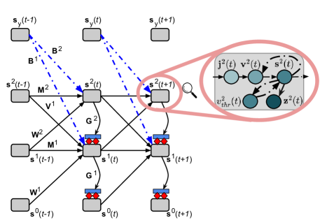
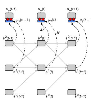
Figure 4: (Left) An overview of the circuit architecture of our CSDP-adapted recurrent spiking network, unfolded over three time steps, which processes a sensory spike train $\{\mathbf{s}^{0}(0),...,\mathbf{s}^{0}(t),...,\mathbf{s}^{0}(T)\})$ with possibly an available corresponding context spike train $\{\mathbf{s}_{y}(0),...,\mathbf{s}_{y}(t),...,\mathbf{s}_{y}(T)\})$. The zoomed-in inset depicts, internally, that each activation layer is made up of at least four components, i.e., an electrical current model $\mathbf{j}^{\ell}(t)$, a voltage model $\mathbf{v}^{\ell}(t)$, a spike response function $\mathbf{s}^{\ell}(t)$, and an adaptive threshold $v^{\ell}_{thr}(t)$. Note that the synaptic connections $\mathbf{B}^{1}$ and $\mathbf{B}^{2}$ are shown as dot-dashed blue lines to indicate that they are optional, e.g., in the case there is no available context spike train (unsupervised adapation), they would be omitted. (Right) The circuit is shown predicting the context $\mathbf{s}_{y}(t)$, where at each step $t$, the spiking classifier makes its best guess $\mathbf{\mu}_{y}(t)$ of the context’s spike train and adjusts relevant synapses via an error-driven Hebbian rule.

While the above per-class class process would work fine for reasonable values of $C$, it would not scale well to a high number of classes, i.e., very large values of $C$, given that the above process requires simulating the spiking network over $C$ stimulus windows in order to compute a predicted label index that corresponds to maximum goodness. However, we constructed a simple modification which circumvents the need to conduct this classification process entirely by integrating a simple spiking classification sub-circuit to the recurrent spiking system. This classifier, which takes in as input the spike output produced at the top level of the recurrent system, i.e., $\mathbf{s}^{L}(t)$, is jointly learned with the rest of the model parameters; this merely entails extending $\Theta$ one more time so as to include classification-specific synapses, i.e., $\Theta\bigcup\Theta_{c}$ where $\Theta_{c}=\{\mathbf{A}^{\ell}\}^{L}_{\ell=1}$. Concretely, the classifier module operates according to the following dynamics:

$$\mathbf{v}_{y}(t+\Delta t) =\mathbf{v}_{y}(t)+\frac{\Delta t}{\tau_{m}}\Big{(}-\mathbf{v}_{y}(t)+R_{m}\Big{(}\sum^{L}_{\ell=1}\mathbf{A}^{\ell}\cdot\mathbf{s}^{\ell}(t)\Big{)}\Big{)}$$ (20)

$$\mathbf{\mu}_{y}(t) =\mathbf{v}_{y}(t+\Delta t)>v^{y}_{thr},\;\mathbf{v}_{y}(t)=\mathbf{v}_{y}(t+\Delta t)\odot(1-\mathbf{\mu}_{y}(t))$$ (21)

$$v^{y}_{thr} =v^{y}_{thr}+\lambda_{v}\Big{(}(\sum^{C}_{j=1}\mathbf{\mu}_{y,j}(t)-1\Big{)}$$ (22)

where we notice, in Equation 20, that the contextual prediction voltage $\mathbf{v}_{y}(t)$ is the result of aggregating across the spike vector messages transmitted from layers $\ell=1$ to $\ell=L$. Each synaptic matrix $\mathbf{A}^{\ell}$ that makes up the spiking classifier is adjusted according to the following Hebbian rule:

$$\Delta\mathbf{A}^{\ell}=\big{(}\mathbf{\mu}_{y}(t)-\mathbf{s}_{y}(t)\big{)}\cdot(\mathbf{s}^{\ell}(t))^{T}\mbox{.}$$ (23)

If these additional synaptic classification parameters are learned, then, at test time, when synaptic adjustment would be disabled/turned off, one can simply provide the spiking system with the sensory input $\mathbf{x}$ with no context $\mathbf{y}$ and obtain a estimated context output $\mathbf{\bar{y}}$. This $\mathbf{\bar{y}}$ is a function of the system’s predictions/outputs across time, i.e., it is the approximate output/label distribution computed as: $p(\mathbf{y}|\mathbf{x};\Theta)\approx\mathbf{\bar{y}}=\exp(\sum^{T}_{t=1}\mathbf{\mu}_{y}(t))/\sum^{C}_{c=1}\exp(\sum^{T}_{t=1}\mathbf{\mu}_{y}(t))_{c}$. Note that the conditional log likelihood $\log p(\mathbf{y}|\mathbf{x};\Theta)$ of the spiking model can now be measured using this approximate label probability distribution. Although learning this spiking classifier entails a memory cost of up to $L$ additional synaptic matrices, the test-time inference of the spiking system will be significantly faster, thus making it more suitable for on-chip computation.

In Figure 4 (Right), our recurrent spiking neural architecture is shown making predictions of the context’s spike train across three time steps. Finally, in the supplementary material, we formally depict how to simulate our recurrent spiking system, including its classification, reconstruction, and (CSDP) credit assignment processes, when processing an input pattern.

3 Experiments

Table 1: Measurements of generalization error of spiking networks trained with different credit assignment processes (means and standard deviations reported for $10$ trials). “Imp.” denotes implementation. BP-FFN is the rate-coded comparison model (a backprop-trained feedforward neural network).

	MNIST	K-MNIST
BP-FNN	$1.300\pm 0.023$	$6.340\pm 0.202$
Spiking-RBM [48]	$11.000$	–
SNN-LM [23]	$5.930$	–
Power-Law STDP [13]	$5.000$	–
DRTP [18] (Imp.)	$6.451\pm 0.172$	$21.320\pm 0.130$
BFA [78] (Imp.)	$3.352\pm 0.102$	$11.250\pm 0.050$
L2-SigProp [33] (Imp.)	$11.425\pm 0.0152$	$29.065\pm 0.013$
Loc-Pred [50] (Imp.)	$6.240\pm 0.034$	$24.820\pm 0.203$
CSDP, Unsup (Ours)	$3.770\pm 0.045$	$9.403\pm 0.106$
CSDP, Sup (Ours)	$2.540\pm 0.030$	$8.860\pm 0.021$

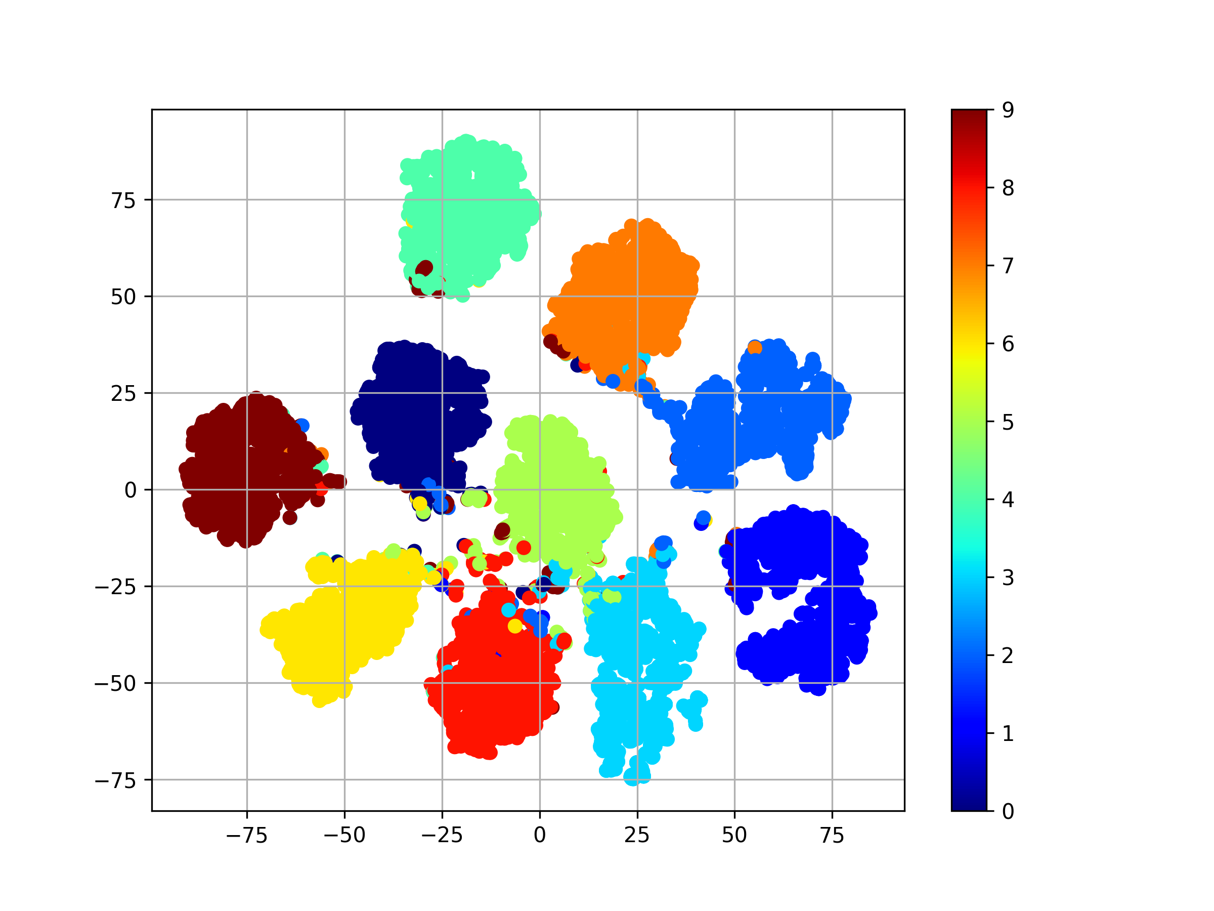
(a) MNIST latents (CSDP, Sup).

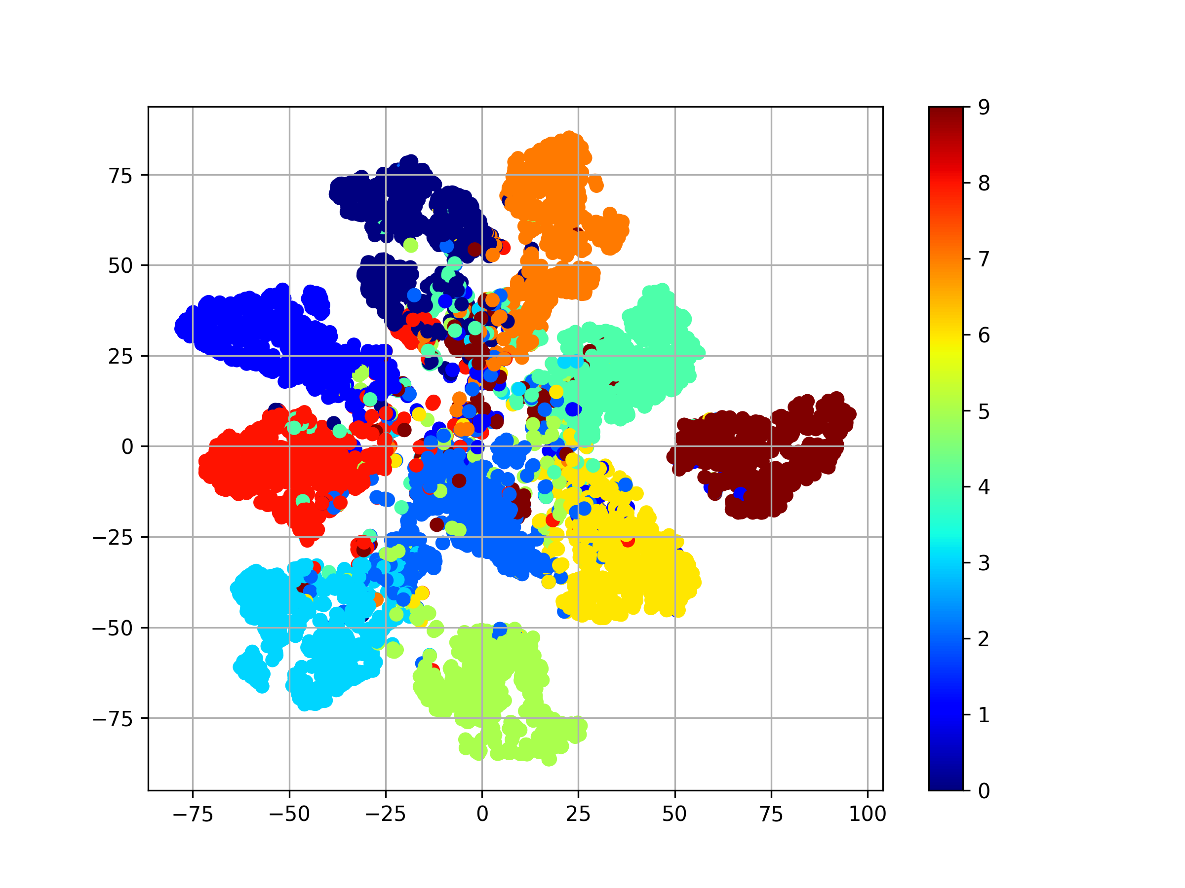
(b) K-MNIST latents (CSDP, Sup).

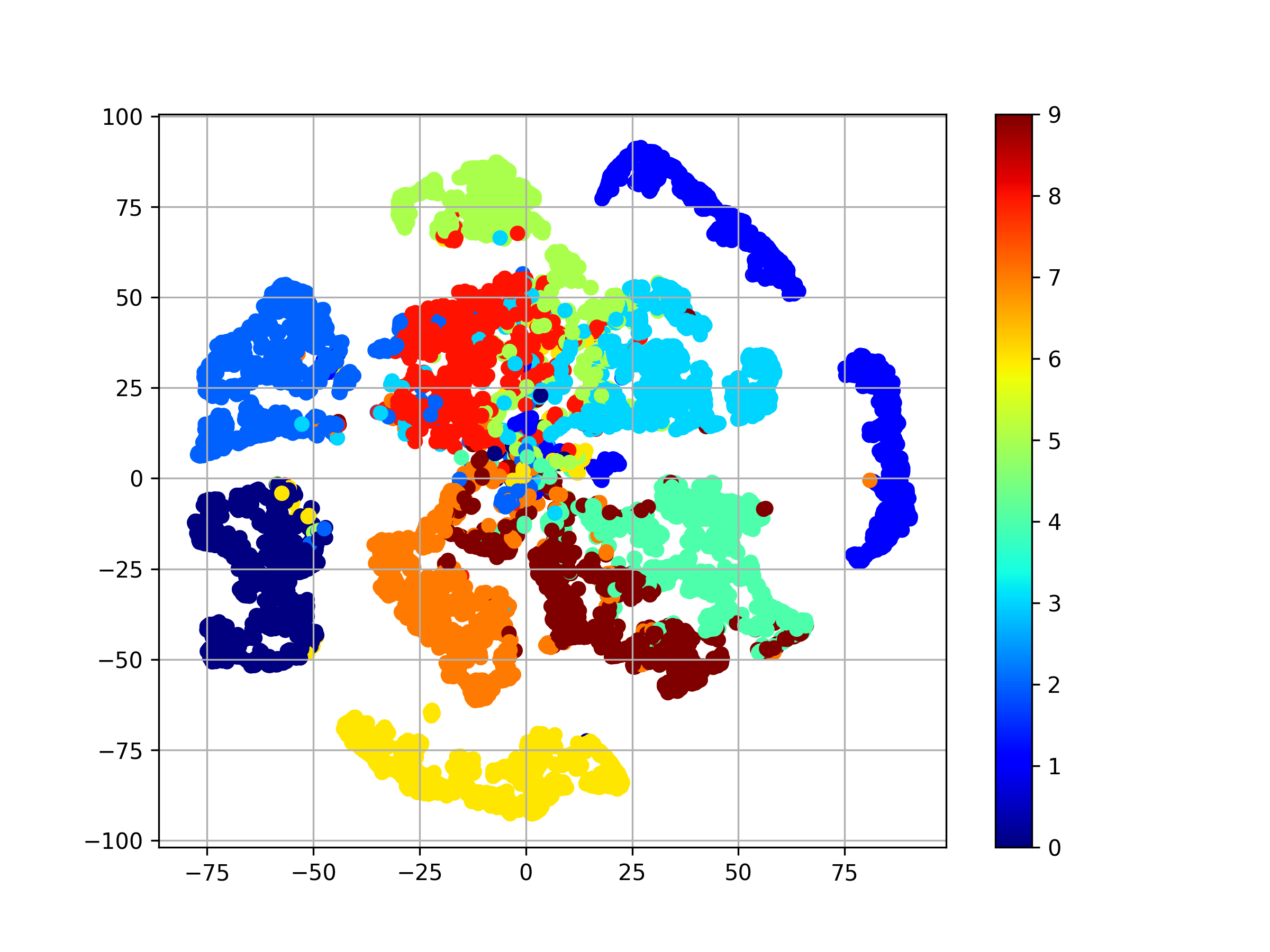
(c) MNIST latents (CSDP, Unsup).

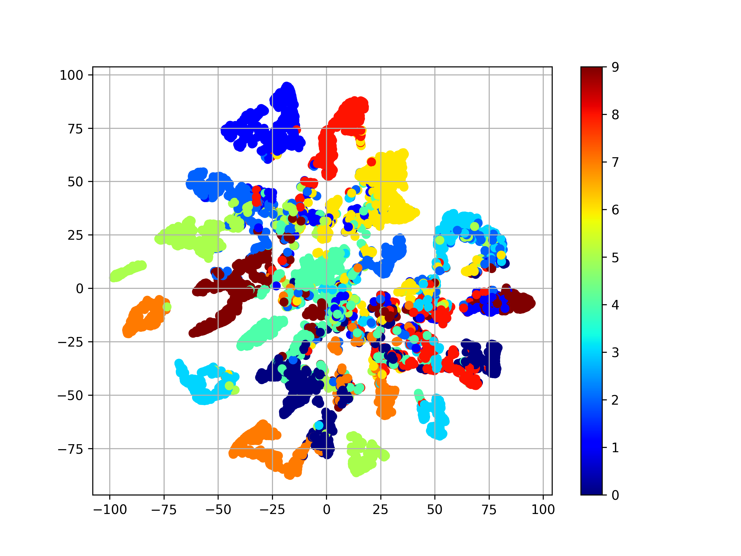
(d) K-MNIST latents (CSDP, Unsup).

Figure 5: t-SNE visualizations of the latent space induced by recurrent spiking networks learned with the CSDP process. (Left) MNIST rate codes are visualized. (Right) K-MNIST rate codes are visualized. Top row shows latent codes uncovered by supervised context-driven SNNs (‘CSDP, Sup’) while the bottom row presents those extracted from unsupervised SNNs (‘CSDP, Unsup’).

3.1 Experimental Setup

Datasets. The MNIST dataset [40] specifically contains images of handwritten digits across $10$ different categories. Kuzushiji-MNIST (K-MNIST) is a challenging drop-in replacement for MNIST, containing images depicting hand-drawn Japanese Kanji characters [8]; each class in this database corresponds to the character’s modern hiragana counterpart, with $10$ total classes. For both datasets, image patterns were normalized to the range of $[0,1]$ by dividing pixel values by $255$. The resulting pixel “probabilities” were then used to create sensory input spike trains by treating the normalized vector $\mathbf{x}/255$ as the parameters for a multivariate Bernoulli distribution. The resulting distribution was sampled at each time step $t$ over the stimulus window of length $T$. Note that we did not preprocess the image data any further unlike many previous efforts related to spiking neural networks. However, we remark that it might be possible to obtain better performance by whitening image patterns (particularly in the case of natural images) or applying a transformation that mimics the result of neural encoding populations based on Gaussian receptive fields.

Simulation Details. We compare both unsupervised and supervised SNN model variants adapted via CSDP – ‘CSDP, Unsup’ and ‘CSDP, Sup’, respectively – with several previously reported STDP-adapted SNN results as well as several implemented spiking network baselines: 1) a spiking network classifier trained with direct random target propagation (DTRP) [18], 2) a spiking network trained with broadcast feedback alignment (BFA) [78], 3) a spiking network trained with a simplified variant of signal propagation [34, 33] using a voltage-based rule and a local cost based on the Euclidean (L2) distance function (L2-SigProp), and 4) a spiking network trained using a generalization of local classifiers/predictors, where each layer-wise classifier, instead of being held fixed, is learned jointly with the overall neural system [50, 93] (Loc-Pred). Furthermore, we provide a rate-coded baseline model (i.e., one that does not operate with spike trains) represented by a tuned feedforward neural network trained by backprop (BP-FNN). Notably, SNNs learned via BFA, DRTP, or Loc-Pred require additional neural circuitry in order to create either feedback loops or layer-wise local predictors.

The network models simulated under each learning algorithm were designed to have two latent/hidden layers of $7000$ leaky integrate-and-fire (LIF) neurons with synaptic connection efficacies randomly initialized from a standard Gaussian distribution truncated to the range of $[-1,1]$) (except for the lateral synapses in CSDP, which were truncated to $[0,1]$). All SNN models further employed a spiking classifier of the same design (aggregating the spike vector outputs across all layers) as the one proposed for our CSDP SNN system in order to ensure a fair comparison; we found these hidden-to-output synapses improved generalization performance across the board.

Since all of the credit assignment algorithms, including our own, could support mini-batch calculations, we train all models with mini-batches of $200$ patterns, randomly sampled without replacement from a training dataset, to speed up simulation and used the Adam adaptive learning rate [32] (with step size $\eta=0.002$) to physically adjust synaptic strength values utilizing the updates provided by any one of the simulated algorithms. Each data point/batch $(\mathbf{x},\mathbf{y})$ was presented to all spiking networks (except for ‘CSDP, Unsup’, which only received $\mathbf{x}$) for a stimulus window of $T=30-50$ steps, or between $90$ and $150$ ms, given $\Delta t=3$ ms. Finally, note that all spiking networks employed the same adaptive threshold update scheme that the CSDP system used – it was observed that this mechanism improved training stability in all cases.

Synthesizing Negative Patterns. Given that CSDP inherently centers around self-supervised contrastive adaptation, a process for producing negative data patterns to contrast with encountered sensory patterns must be provided. Given that we have developed two different framings of our recurrent neural system – a supervised context-driven form as well as an unsupervised variant – we designed two schemes for generating out-of-distribution/negative data points that specifically operated on-the-fly, i.e., only utilized information/statistics within a current batch of data. In the case of the supervised context-driven model, we adapted the scheme used in [26, 63]; for each $(\mathbf{y},\mathbf{x})$ in a mini-batch/pool of patterns, we would produce a negative batch $(\mathbf{y}^{-},\mathbf{x}^{-})$ by duplicating the original images and, for each cloned (original/positive) pattern, we then created a corresponding ‘incorrect’ paired label by randomly sampling a class index other than the correct one (index $c$) found within $\mathbf{y}$. For the unsupervised variant, where $\mathbf{y}=\emptyset$, we took inspiration from [92] and designed a simple on-the-fly process that applied the following steps to a current mini-batch of patterns: 1) for each pattern $\mathbf{x}_{i}$, we would select one other different pattern $\mathbf{x}_{j}$, $j\neq i$, within the batch, 2) apply a random rotation to $\mathbf{x}_{j}$ (by sampling a rotation value, in radians, from the range $(\frac{\pi}{4},\frac{7\pi}{4}$) to create $\mathbf{r}_{j}$, and finally, 3) produce a negative pattern via the convex combination $\mathbf{x}^{-}_{i}=\eta\mathbf{x}_{i}+(1-\eta)\mathbf{r}_{j}$ with $\eta=0.55$ ($\eta$ interpolates between the original and rotated, non-original pattern).

3.2 Model Performance Results

In Table 1, we present our simulation results for our recurrent spiking model trained with CSDP. Notice that, like many bio-physical spiking networks, even though we do not quite match the performance of backprop-based feedforward networks, our generalization error comes surprisingly close. This is particularly promising given that the predicted context layer is a layer of spiking neurons itself. Furthermore, our CSDP model, particularly the supervised context-driven variant ‘CSDP, Sup’, comes the closest to matching the BP-FNN rate-coded baseline compared to the other SNN credit assignment algorithms. The unsupervised CSDP model only does slightly worse than the supervised one and effectively operates on par with the BFA-adapted SNN on MNIST (yet outperforms it on K-MNIST). The BFA SNN offers a competitive baseline, illustrating that feedback synapses are still quite a powerful mechanism (outperforming methods such as Loc-Pred and L2-SigProp) even though this work’s goal was to demonstrate effective learning without feedback.

In Figure 5, we examine the clusters that emerge within the latent space induced by recurrent spiking networks trained with CSDP. To compute the latent vectors/codes, we formed an approximate rate code from the top layer spike train, i.e., $\{\mathbf{s}^{L}\}^{T}_{t=1}$, of the system produced by each data point as follows:

$$\mathbf{c}=\frac{\gamma_{c}}{T}\sum^{T}_{t}\mathbf{s}^{L}_{t}$$ (24)

with $\gamma_{c}=1$. After feeding each data point $\mathbf{x}$ (without its context $\mathbf{y}$) in the test-set to each model and collecting an approximate top-layer rate-code vector $\mathbf{c}$, we visualized the emergent islands of rate codes using t-Distributed Stochastic Neighbor Embedding (t-SNE) [88]. Notice how, for both MNIST (Figure 5(a)) and K-MNIST (Figure 5(b)), clusters related to each category naturally form, qualitatively demonstrating why CSDP-adapted spiking models are able to classify unseen test patterns effectively. This is particularly impressive for K-MNIST, which is arguably the more difficult of the two datasets, which means that CSDP adaptation is capable of extracting class-centric information from more complicated patterns. Note, as expected, the clusters are less separated and distinct in the case of the unsupervised model variant ‘CSDP, Unsup’.

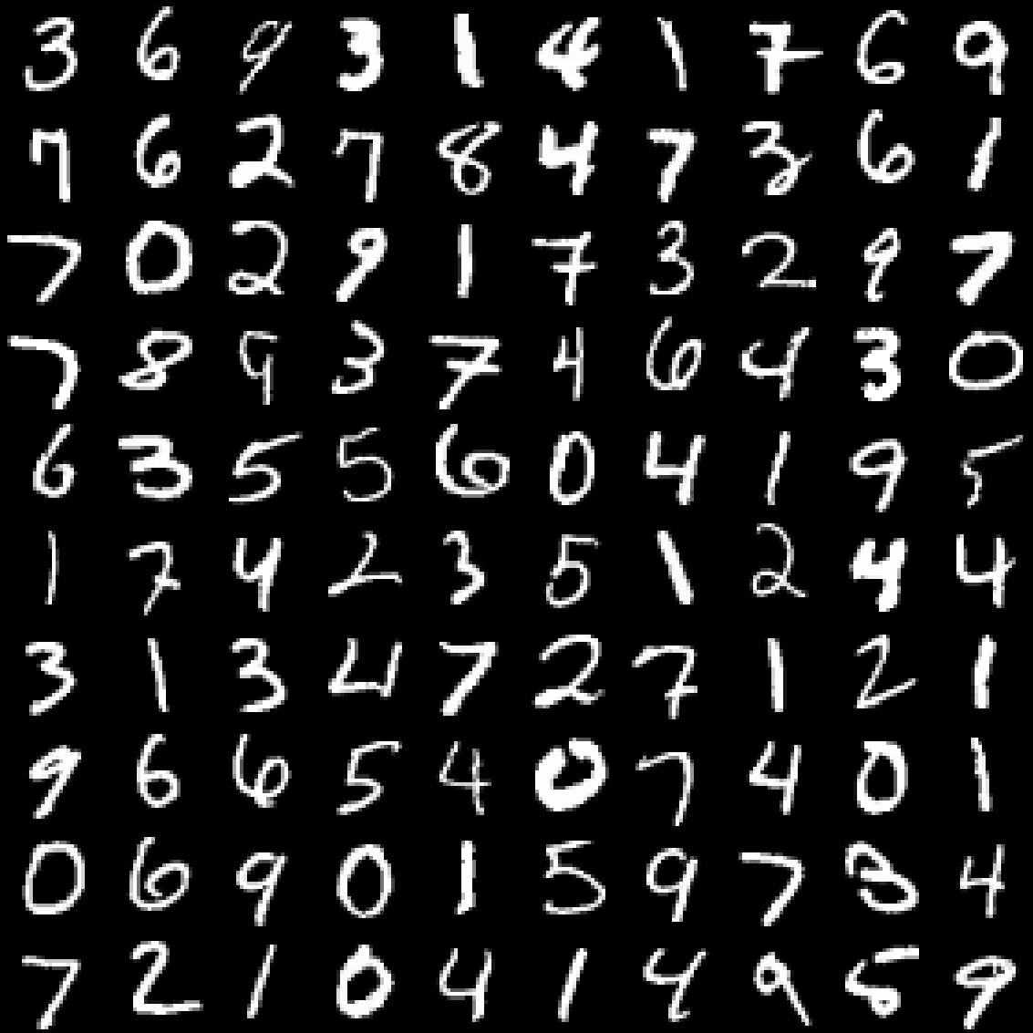
(a) MNIST data samples.

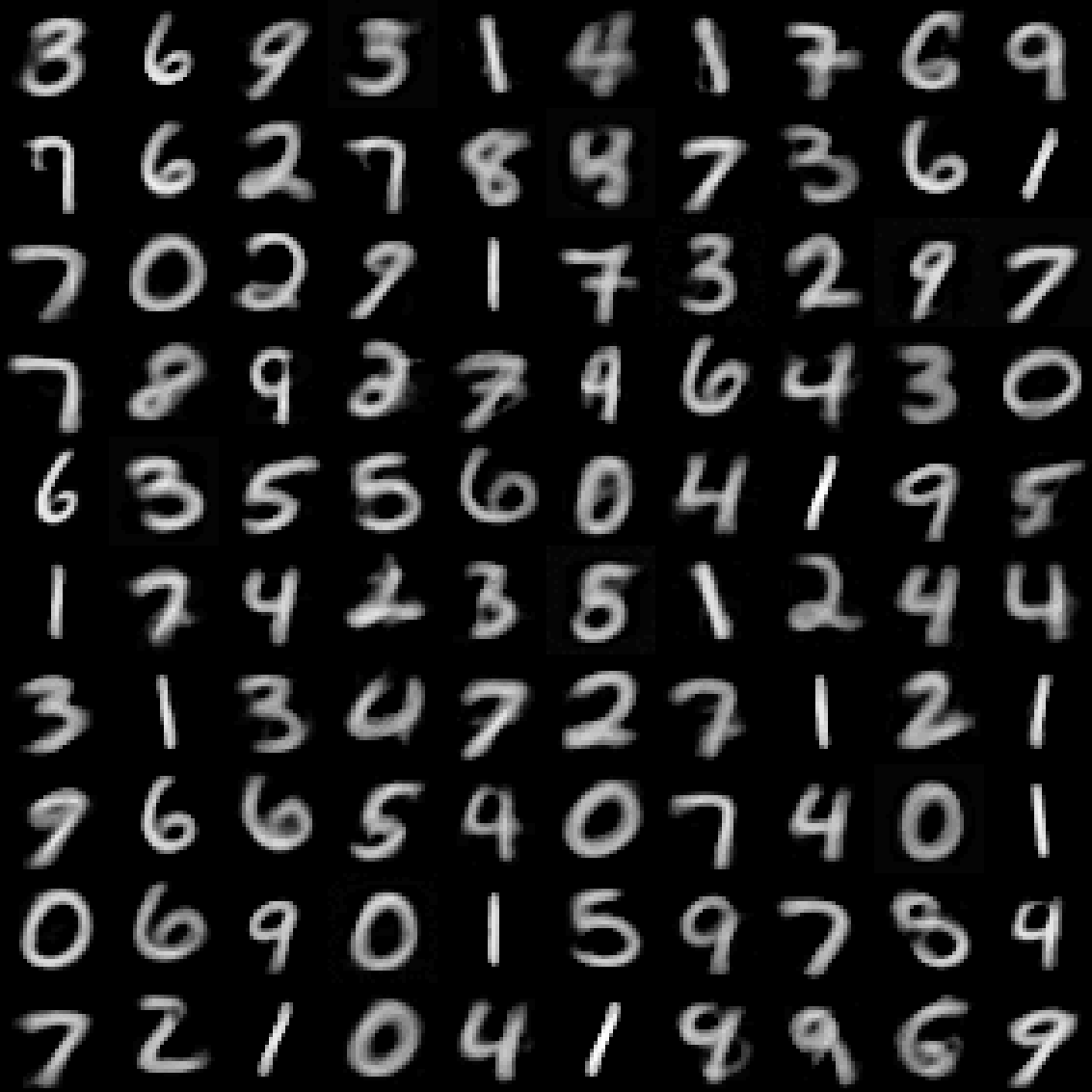
(b) MNIST reconstruction.

(c) K-MNIST data samples.

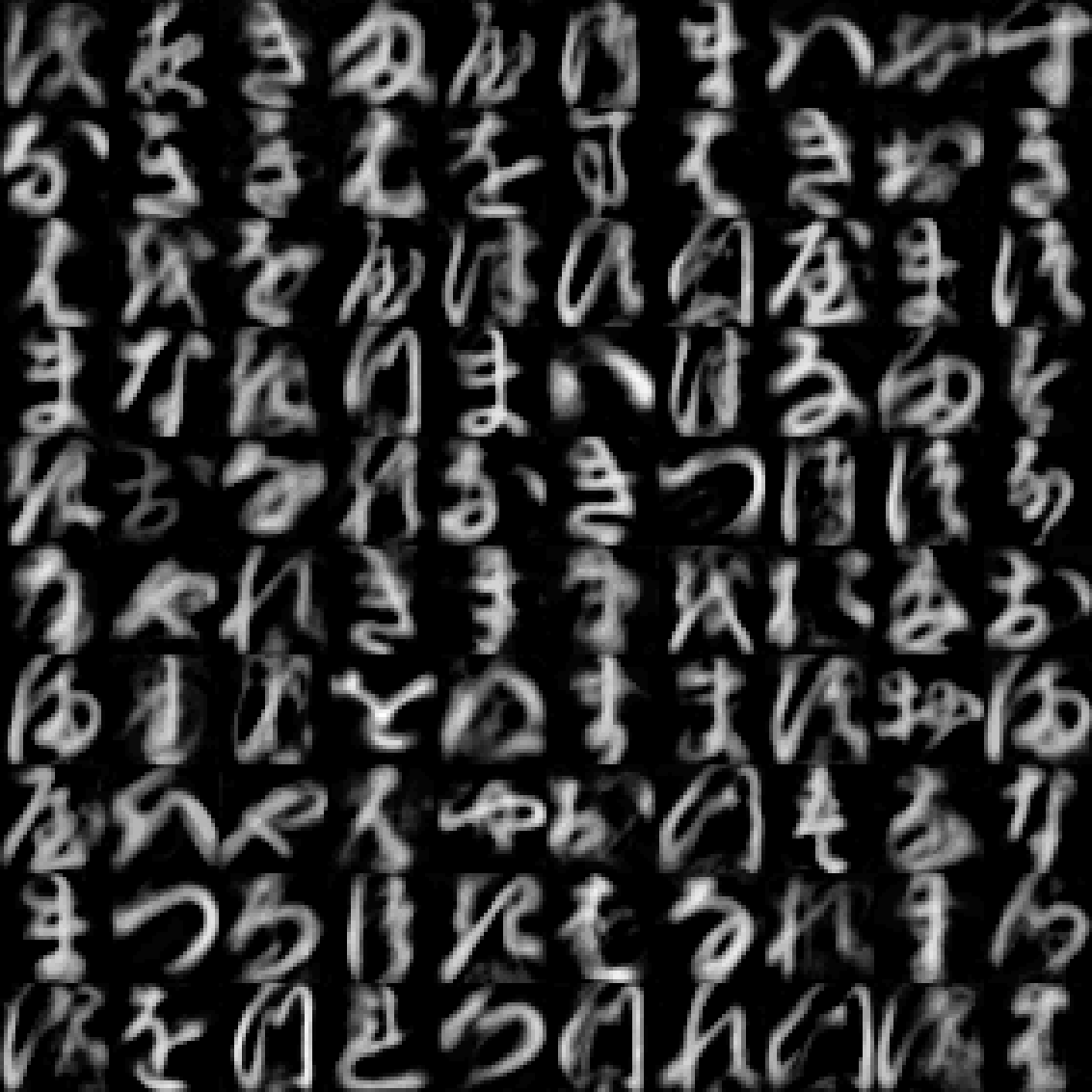
(d) K-MNIST reconstruction.

Figure 6: Reconstructions produced by the SNN when learned with CSDP. Left column (sub-figures a and c) present the randomly selected images from the target database while the right column (sub-figures b and d) present the reconstructed patterns produced by the recurrent spiking model. Top row presents results for MNIST while the bottom row presents results for K-MNIST.

Pattern Reconstruction. In Figure 6, we examine the pattern reconstruction ability of a CSDP spiking model (focusing on the ‘CSDP, Sup’ variant) on randomly sampled, without replacement, image patterns from the MNIST and K-MNIST databases. A single reconstructed pattern $\mathbf{\widehat{x}}$ was created by computing an average across activation traces of the bottom-most predictor’s output spikes, collected during the $T$-length stimulus window as follows:

$$\mathbf{\widehat{x}} =\frac{1}{T}\sum^{T}_{t=1}\mathbf{z}^{0}_{\mu}(t),\;\mbox{where }\mathbf{z}^{0}_{\mu}(t)=\mathbf{s}^{0}_{\mu}(t)-\frac{\Delta t}{\tau_{tr}}\mathbf{z}^{0}_{\mu}(t)\odot(1-\mathbf{z}^{0}_{\mu}(t))$$ (25)

where $\mathbf{z}^{0}_{\mu}(t)$ is the activation trace of the output prediction spike vector $\mathbf{s}^{0}_{\mu}(t)$, produced by the local prediction of layer $\ell=0$ from layer $\ell=1$ (see Equation 13), at simulation step $t$.

Desirably, we see that the CSDP model is able to produce reasonable reconstructions of the image patterns, demonstrating that it is enable to encode in its generative synapses information that is useful for decoding from the very sparse spike train representations that characterize its internal layers of LIF neurons. Note that the context $\mathbf{y}$ was not clamped to our model when reconstruction ability was evaluated; this means that the model had to employ any contextual information it had stored into its synapses in order to determine how to best reconstruct test samples.

Patch-Level Representations. We finally briefly investigate the representation capability of our spiking system in the context of image patches. Specifically, we extracted patches of $8\times 8$ and $12\times 12$ pixels from a subset of the MNIST database ($1000$ image patterns, $10$ from each class) and trained a model with $2000$ LIF units in both layers using the CSDP procedure. The learned receptive fields, for each of the two patch settings, of the bottom-most layer of the trained model, i.e., layer $\ell=1$, are shown in Figure 7. Receptive fields in the bottom layer were extracted for visualization by randomly sampling, without replacement, $100$ slices of the synaptic matrix $\mathbf{W}^{1}$. As observed in Figure 7, the receptive fields extract basic patterns at different resolutions; in the smaller $8\times 8$ patch model, we see simpler patterns emerge such as edges or stroke pieces (“strokelets”) of different orientations while in the larger $12\times 12$ patch model we observe portions of patterns that appear as “mini-templates” that could be used to compose larger digits.

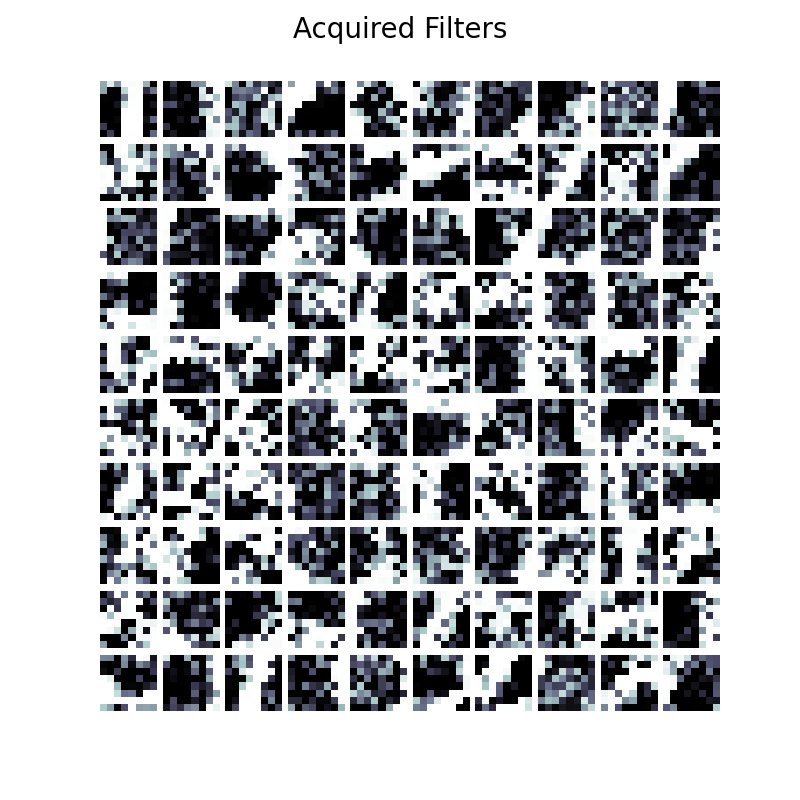
(a) $8\times 8$ patch model.

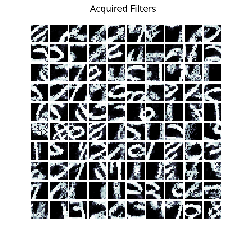
(b) $12\times 12$ patch model.

Figure 7: The receptive fields of $100$ randomly chosen LIF neurons, in layer $\ell=1$, of unsupervised CSDP models, trained on patches. Shown are the receptive fields for: (Left) $8\times 8$ patches, and (Right) $12\times 12$ patches.

3.3 Discussion

On Limitations. Although our online contrastive forward-only credit assignment process for training recurrent spiking networks is promising, there are several limitations to consider. First, although the spiking model that we designed operates with bounded synaptic values (between $-1,1$), it does not operate with strictly positive values, which is an important hallmark of neurobiology – we cannot have negative synaptic efficacies. This is an unfortunate limitation that is made worse by the fact that the signs of the synaptic values could change throughout the course of simulated learning. Nevertheless, we remark that this issue could be potentially rectified by constraining all synapses to $[0,1]$ and then introducing an additional set of spiking inhibitory (or inter-inhibitory) neurons coupled to each layer which would provide the inhibitory/depression signals generally offered by negative synaptic strengths. The proportion of inhibitory neurons to excitatory ones could then be desirably configured to furthermore adhere to Dale’s Law [84]. Future work will explore this possible reformulation, as the countering pressure offered by negative synapses is important for a goodness-based contrastive objective, much as the one employed by CSDP, to work properly – ideally, inhibitory neurons should provide a similar type of pressure.

Beyond its use of synapses without a sign constraint, our current recurrent SNN does not include refractory periods, only implementing an instantaneous form of depolarization for all NPEs. However, this could be easily corrected by modifying Equation 3 to include an absolute refractory period, as in [59], as well as a relative refractory period. Furthermore, the adaptive thresholds we presented in Equations 4, 16, and 22 are each calculated as a function of the total number of spikes across a layer $\ell$, at time $t$, whereas it would be more bio-physically realistic to have each LIF unit within a layer adapt its own specific scalar threshold.

Finally, with respect to the contrastive-signal-dependent plasticity process itself, while we were able to desirably craft a simple update rule that operated at the spike-level, via a biologically plausible activation trace, there is still the drawback that the rule, much like its rated-coded sources of inspiration [26, 63], requires positive and negative data samples to compute useful synaptic adjustments. In this study, we made use of two simple approaches to synthesize negative samples: 1) in the case of the supervised context model variant, we exploited the fact that labels were readily available to serve as top-down context signals which made synthesizing negative samples easy – all we needed to do was simply select one of the incorrect class labels to create a negative context, or 2) generated out-of-distribution patterns by interpolating between distinct pattern pairs within a mini-batch in tandem with randomly applied (image) rotation. However, while our approaches for synthesizing negative data samples are simple and online, investigating alternative, more sophisticated schemes would prove fruitful. One promising way to do this could be through the use of the predictive/generative synapses of the CSDP spike model we introduced earlier; the system could dynamically produce data confabulations that could serve as on-the-fly negative patterns. However, the greatest difficulty in synthesizing negative samples through the generative circuitry of our spiking model would be in crafting a process by which ancestral sampling could be efficiently conducted. For the supervised variant of our model, an alternative to synthesizing negative samples would be to design another neural circuit that produces context vector $\mathbf{y}$ (both positive and negative variations) instead of using a provided label – a direction that is also more biologically realistic. Another drawback of using positive and negative samples in the kind of contrastive learning that we do in this work is that both types of data are used simultaneously. In [26, 63], it has been discussed that it will be important to examine alternative schedules for when negative samples are presented to and used by a neural system to adjust its synapses.

3.4 Related Work

Backprop has long faced criticism with respect to its neurobiological plausibility [11, 21, 81, 47, 22]; it is unlikely that backprop is a viable model of credit assignment in the brain. Among the biophysical issues [22, 47] that plague backprop, some of the key ones include: 1) neural activities are explicitly stored to be used later for synaptic adjustment, 2) error derivatives are backpropagated along a global feedback pathway [65] in order to generate useful teaching signals, 3) the error signals move back along the same neural pathways used to forward propagate information (also known as the weight transport problem [22]), and, 4) inference and learning are locked to be largely sequential [30] (instead of massively parallel as in the brain), and 5) when processing temporal data, unfolding of the neural circuitry backward through time (i.e., backprop through time) is necessary before adjusting the synaptic weight values (which is clearly not the case for brain-like computation [64, 46]).

Recently, there has been a growing interest in developing algorithms and computational models that attempt to circumvent or resolve some of the criticisms highlighted above. Among the most powerful and promising ones is predictive coding (PC) [25, 73, 19, 3, 76, 62], and among the most recent ones is forward-only learning, including approaches such as signal propagation [34, 33]), the forward-forward (FF) algorithm [26], and the predictive forward-forward (PFF) procedure [63]. These alternatives offer mechanisms for conducting credit assignment that are more consistent with elements of neurobiological learning while empirically exhibiting performance similar to backprop. Crucially, evidence has been found in support of the principles underlying self-supervised contrastive learning, such as those that characterize forward-only schemes such as our proposed CSDP, with respect to biophysical neuronal functionality [39, 35, 28, 36, 52].

Forward-only processes [34, 26, 63] have a unique advantage over other biological credit assignment schemes in that they only require forward propagation of information to facilitate learning, resulting in synaptic updates that are in the same spirit as Hebbian learning [24]. In addition, such processes are more suitable for on-chip learning (for neuromorphic hardware) given that they do not require distinct separate computational pathway(s) for transmitting teaching signals (which is required by backprop [75] and feedback alignment methods [42, 53]) or even error messages and error transmission pathways, which are required by predictive coding [73, 3, 62], representation alignment [68], and target propagation processes [41]. Desirably, this means that no specialized hardware is needed for computing activation function derivatives nor for maintaining and adjusting separate feedback transmission synapses that often require different adjustment rules [68, 64]. In addition, forward-only rules are generally faster than adaptation processes based on contrastive Hebbian learning [51, 27, 79], given that they do not require a negative phase computation that is conditioned on the statistics of a positive one (or vice versa). Finally, a forward-only scheme such as CSDP naturally allows for incorporation of lateral competition within its layer-wise activities, offering corroborating evidence that cross-inhibitory activity patterns [89, 57, 66] are important for neural computation; note that competitive learning has proven valuable when integrated with pure STDP-centric adaptation [82] and further plays an important role in CSDP-adapted recurrent SNNs.

4 Conclusion

In this work, we presented the contrastive-signal-dependent plasticity (CSDP) process, a generalization of forward-forward learning to the case of spike trains, for adjusting the synaptic efficacies of a recurrent spiking neural systems. Experimentally, we demonstrated that CSDP adaptation could successfully learn discrete temporal representations that facilitated effective classification of image data as well as reconstruct the image inputs over time. Among the many potential directions that merit exploration with respect to CSDP credit assignment, we believe that investigating how the adaptation process would operate in the context of far more complex data, such as natural images (assuming that the spiking system was equipped with the proper inductive biases) and sequences, e.g., video frames, will be important. Furthermore, it would be interesting to observe how spike-level circuitry, adapted via CSDP learning, might be useful for neural-centric cognitive architectures [60, 61, 67], inspired by the success of models such as the Semantic Pointer Architecture (SPAUN) [85].

Acknowledgements

We would like to thank Alexander Ororbia (Sr.) for useful feedback on the early draft of the manuscript.

Supplementary Material

Simulating a CSDP-Adapted Spiking Recurrent Circuit

In this section, we provide the full pseudocode required for simulating a recurrent spiking network of arbitrary depth processing an input pattern over an arbitary-length stimulus window. Note that Algorithm 1 depicts both supervised context-driven and unsupervised variations of our modeling framework.

Algorithm 1 The contrastive-signal-dependent plasticity credit assignment algorithm. Blue lines depict portions of the simulation code executed if the supervised variant of the process is to be utilized.

1: Input: sample $(\mathbf{y},\mathbf{x})$ (with $\mathbf{y}=\emptyset$ if unsupervised), SNN parameters $\Theta$, and

2:          virtual data label $y_{type}$ (with value: $1=$ “positive” and $0=$ “negative”)

3: Hyperparameters: SGD step size $\eta$, stimulus time $T$, integration constant $\Delta t$, time constants $\tau_{m}$ and $\tau_{tr}$,

4:                       adaptive threshold step $\lambda_{v}$

5: $//$ $\leftarrow$ denotes the overriding of a variable/object, $\Omega()$ is a bounding function

6: function Simulate($(\mathbf{y},\mathbf{x},y_{type}),\Theta$)

7:      for $t=1$ to $T$ do

8:          $\mathbf{s}^{0}(t)\sim\mathcal{B}(1,p=\mathbf{x})$,   $\mathbf{s}_{y}(t)=\mathbf{y}$ $\triangleright$ Sample sensory input and context to get an input spike at time $t$

9:          for $\ell=1$ to $L$ do

10:               $//$ Compute the current and voltage components of layer $\ell$

11:               if $\ell<L$ then

12:                   $\mathbf{j}^{\ell}(t)=\mathbf{W}^{\ell}\cdot\mathbf{s}^{\ell-1}(t)+\mathbf{V}^{\ell}\cdot\mathbf{s}^{\ell+1}(t)-(\mathbf{M}^{\ell}\odot(1-\mathbf{I}^{\ell}))\cdot\mathbf{s}^{\ell}(t)$

13:               else

14:                   $\mathbf{j}^{\ell}(t)=\mathbf{W}^{\ell}\cdot\mathbf{s}^{\ell-1}(t)-(\mathbf{M}^{\ell}\odot(1-\mathbf{I}^{\ell}))\cdot\mathbf{s}^{\ell}(t)$               

15:               if $\mathbf{y}\neq\emptyset$ then

16:                   $\mathbf{j}^{\ell}(t)=\mathbf{j}^{\ell}(t)+\mathbf{B}^{\ell}\cdot\mathbf{s}_{y}(t)$ $\triangleright$ Apply label context pressure (if supervised)               

17:               $\mathbf{v}^{\ell}(t+\Delta t)=\mathbf{v}^{\ell}(t)+\frac{\Delta t}{\tau_{m}}\Big{(}-\mathbf{v}^{\ell}(t)+R_{m}\mathbf{j}^{\ell}(t)\Big{)}$

18:               $//$ Run the spike model given $\mathbf{j}(t)$ and $\mathbf{v}(t)$ (and depolarize $\mathbf{v}(t)$ if applicable)

19:               $\mathbf{s}^{\ell}(t)=\mathbf{v}^{\ell}(t+\Delta t)>v^{\ell}_{thr}$,   $\mathbf{v}^{\ell}(t)=\mathbf{v}^{\ell}(t+\Delta t)\odot(1-\mathbf{s}^{\ell}(t))$,   $v^{\ell}_{thr}=v^{\ell}_{thr}+\lambda_{v}\big{(}(\sum^{J_{\ell}}_{j=1}$,   $\mathbf{s}^{\ell}(t)_{j})-1\big{)}$

20:               $//$ Update the activation trace for layer $\ell$

21:               $\mathbf{z}^{\ell}_{t}=\mathbf{s}^{\ell}_{t}-\frac{\Delta t}{\tau_{tr}}\mathbf{z}^{\ell}_{t}\odot(1-\mathbf{z}^{\ell}_{t})$

22:               $//$ Calculate local synaptic adjustments and update its synaptic efficacies

23:               Get loss $\mathcal{L}_{G}(\mathbf{z}^{\ell}(t),y_{type})$ (Equation 6) & its partial derivative w.r.t. $\mathbf{z}^{\ell}(t)$, i.e., $\delta^{\ell}(t)=2\frac{\partial\mathcal{L}_{G}(\mathbf{z}^{\ell}(t),y_{type})}{\partial\sum^{J_{\ell}}_{j}(\mathbf{z}^{\ell}_{j}(t))^{2}}$

24:               $\Delta\mathbf{W}^{\ell}=\big{(}R_{m}\delta^{\ell}(t)\cdot\big{(}\mathbf{s}^{\ell-1}(t-1)\big{)}^{T}\big{)}+\lambda_{d}\big{(}\mathbf{s}^{\ell}(t)\cdot(1-\mathbf{s}^{\ell-1}(t))^{T}\big{)}$,   $\mathbf{W}^{\ell}\leftarrow\Omega\big{(}\mathbf{W}^{\ell}-\eta\Delta\mathbf{W}^{\ell}\big{)}$

25:               $\Delta\mathbf{V}^{\ell}=\big{(}R_{m}\delta^{\ell}(t)\cdot\big{(}\mathbf{s}^{\ell+1}(t-1)\big{)}^{T}\big{)}+\lambda_{d}\big{(}\mathbf{s}^{\ell}(t)\cdot(1-\mathbf{s}^{\ell+1}(t))^{T}\big{)}$,   $\mathbf{V}^{\ell}\leftarrow\Omega\big{(}\mathbf{V}^{\ell}-\eta\Delta\mathbf{V}^{\ell}\big{)}$

26:               $\Delta\mathbf{M}^{\ell}=\big{(}R_{m}\delta^{\ell}(t)\cdot\big{(}\mathbf{s}^{\ell}(t-1)\big{)}^{T}\big{)}+\lambda_{d}\big{(}\mathbf{s}^{\ell}(t)\cdot(1-\mathbf{s}^{\ell}(t))^{T}\big{)}$,   $\mathbf{M}^{\ell}\leftarrow\Omega\big{(}\mathbf{M}^{\ell}-\eta\Delta\mathbf{M}^{\ell}\big{)}$

27:               if $\mathbf{y}\neq\emptyset$ then

28:                   $\Delta\mathbf{B}^{\ell}=\big{(}R_{m}\delta^{\ell}(t)\cdot\big{(}\mathbf{s}_{y}(t-1)\big{)}^{T}+\lambda_{d}\big{(}\mathbf{s}^{\ell}(t)\big{)}\cdot(1-\mathbf{s}^{y}(t))^{T}\big{)}$,   $\mathbf{B}^{\ell}\leftarrow\Omega\big{(}\mathbf{B}^{\ell}-\eta\Delta\mathbf{B}^{\ell}\big{)}$               

29:               $//$ Run $\ell$th local predictor, error neurons and adjust its synaptic efficacies

30:               $\mathbf{v}^{\ell}_{\mu}(t+\Delta t)=\mathbf{v}^{\ell}_{\mu}(t)+\frac{\Delta t}{\tau_{m}}\Big{(}-\mathbf{v}^{\ell}_{\mu}(t)+R_{m}(\mathbf{G}^{\ell+1}\cdot\mathbf{s}^{\ell+1}(t))\Big{)}$

31:               $\mathbf{s}^{\ell}_{\mu}(t)=\mathbf{v}^{\ell}_{\mu}(t+\Delta t)>v^{\ell}_{thr,\mu}$,   $\mathbf{v}^{\ell}_{\mu}(t)=\mathbf{v}^{\ell}_{\mu}(t+\Delta t)\odot(1-\mathbf{s}^{\ell}_{\mu}(t))$,   $v^{\ell}_{thr,\mu}=v^{\ell}_{thr,\mu}+\lambda_{v}\big{(}(\sum^{J_{\ell}}_{j=1}\mathbf{s}^{\ell}_{\mu,j}(t))-1\big{)}$

32:               $\mathbf{e}^{\ell}(t)=\mathbf{s}^{\ell}_{\mu}(t)-\mathbf{s}^{\ell}(t)$ $\triangleright$ Calculate the error/mismatch activities

33:               $\Delta\mathbf{G}^{\ell}=\big{(}R_{m}\mathbf{e}^{\ell-1}(t)\big{)}\cdot(\mathbf{s}^{\ell}(t))^{T}$,   $\mathbf{G}^{\ell}\leftarrow\Omega\big{(}\mathbf{G}^{\ell}-\eta\Delta\mathbf{G}^{\ell}\big{)}$          

34:          if $\mathbf{y}\neq\emptyset$ then

35:               $//$ Calculate classifier outputs and adjust its synaptic efficacies (if supervised)

36:               $\mathbf{v}_{y}(t+\Delta t)=\mathbf{v}_{y}(t)+\frac{\Delta t}{\tau_{m}}\big{(}-\mathbf{v}_{y}(t)+R_{m}(\sum^{L}_{\ell=1}\mathbf{A}^{\ell}\cdot\mathbf{s}^{\ell}(t))\big{)}$

37:               $\mathbf{\mu}_{y}(t)=\mathbf{v}_{y}(t+\Delta t)>v^{y}_{thr}$,  $\mathbf{v}_{y}(t)=\mathbf{v}_{y}(t+\Delta t)\odot(1-\mathbf{\mu}_{y}(t))$,  $v^{y}_{thr}=\mathbf{\mu}_{y}(t)+\lambda_{v}\big{(}(\sum^{C}_{j=1}\mathbf{\mu}_{y,j}(t)-1\big{)}$

38:               $\Delta\mathbf{A}^{\ell}=\big{(}\mathbf{\mu}_{y}(t)-\mathbf{s}_{y}(t)\big{)}\cdot(\mathbf{s}^{\ell}(t))^{T}$,   $\mathbf{A}^{\ell}\leftarrow\Omega\big{(}\mathbf{A}^{\ell}-\eta\Delta\mathbf{A}^{\ell}\big{)},\;\forall\ell=1...L$

39:          else

40:               $\{\mathbf{A}^{\ell}=\emptyset\}^{L}_{\ell=1}$ $\triangleright$ In unsupervised model, these parameters are set to empty/null values                

41:      Return $\Theta=\{\mathbf{W}^{\ell},\mathbf{V}^{\ell},\mathbf{M}^{\ell},\mathbf{B}^{\ell}\}^{L}_{\ell=1}\bigcup\{\mathbf{G}^{\ell}\}^{L}_{\ell=1}\bigcup\{\mathbf{A}^{\ell}\}^{L}_{\ell=1}$ $\triangleright$ Output newly updated model parameters

References

- [1] Amodei, D., and Hernandez, D. AI and compute. https://openai.com/blog/ai-and-compute/, May 2018.
- [2] Ballard, D. H., Rao, R. P., and Zhang, Z. A single-spike model of predictive coding. Neurocomputing 32 (2000), 17–23.
- [3] Bastos, A. M., Usrey, W. M., Adams, R. A., Mangun, G. R., Fries, P., and Friston, K. J. Canonical microcircuits for predictive coding. Neuron 76, 4 (2012), 695–711.
- [4] Bi, G.-q., and Poo, M.-m. Synaptic modifications in cultured hippocampal neurons: dependence on spike timing, synaptic strength, and postsynaptic cell type. Journal of neuroscience 18, 24 (1998), 10464–10472.
- [5] Brevini, B. Black boxes, not green: Mythologizing artificial intelligence and omitting the environment. Big Data & Society 7, 2 (2020), 2053951720935141.
- [6] Bubeck, S., Chandrasekaran, V., Eldan, R., Gehrke, J., Horvitz, E., Kamar, E., Lee, P., Lee, Y. T., Li, Y., Lundberg, S., et al. Sparks of artificial general intelligence: Early experiments with gpt-4. arXiv preprint arXiv:2303.12712 (2023).
- [7] Caulfield, H. J., Kinser, J., and Rogers, S. K. Optical neural networks. Proceedings of the IEEE 77, 10 (1989), 1573–1583.
- [8] Clanuwat, T., Bober-Irizar, M., Kitamoto, A., Lamb, A., Yamamoto, K., and Ha, D. Deep learning for classical japanese literature, 2018.
- [9] Clark, A. Surfing uncertainty: Prediction, action, and the embodied mind. Oxford University Press, 2015.
- [10] Covi, E., Donati, E., Liang, X., Kappel, D., Heidari, H., Payvand, M., and Wang, W. Adaptive extreme edge computing for wearable devices. Frontiers in Neuroscience 15 (2021), 611300.
- [11] Crick, F. The recent excitement about neural networks. Nature 337, 6203 (1989), 129–132.
- [12] Devlin, J., Chang, M.-W., Lee, K., and Toutanova, K. Bert: Pre-training of deep bidirectional transformers for language understanding. arXiv preprint arXiv:1810.04805 (2018).
- [13] Diehl, P. U., and Cook, M. Unsupervised learning of digit recognition using spike-timing-dependent plasticity. Frontiers in computational neuroscience 9 (2015), 99.
- [14] Duvillier, J., Killinger, M., Heggarty, K., Yao, K., et al. All-optical implementation of a self-organizing map: a preliminary approach. Applied optics 33, 2 (1994), 258–266.
- [15] Eliasmith, C., and Anderson, C. H. Neural engineering: Computation, representation, and dynamics in neurobiological systems. MIT press, 2004.
- [16] Eliasmith, C., Stewart, T. C., Choo, X., Bekolay, T., DeWolf, T., Tang, Y., and Rasmussen, D. A large-scale model of the functioning brain. science 338, 6111 (2012), 1202–1205.
- [17] Floridi, L., and Chiriatti, M. Gpt-3: Its nature, scope, limits, and consequences. Minds and Machines 30, 4 (2020), 681–694.
- [18] Frenkel, C., Lefebvre, M., and Bol, D. Learning without feedback: Direct random target projection as a feedback-alignment algorithm with layerwise feedforward training. arXiv preprint arXiv:1909.01311 (2019).
- [19] Friston, K. The free-energy principle: a unified brain theory? Nature reviews neuroscience 11, 2 (2010), 127–138.
- [20] Furber, S. Large-scale neuromorphic computing systems. Journal of neural engineering 13, 5 (2016), 051001.
- [21] Gardner, D. The Neurobiology of neural networks. MIT Press, 1993.
- [22] Grossberg, S. Competitive learning: From interactive activation to adaptive resonance. Cognitive science 11, 1 (1987), 23–63.
- [23] Hazan, H., Saunders, D., Sanghavi, D. T., Siegelmann, H., and Kozma, R. Unsupervised learning with self-organizing spiking neural networks. In 2018 International Joint Conference on Neural Networks (IJCNN) (2018), IEEE, pp. 1–6.
- [24] Hebb, Donald O, e. a. The organization of behavior, 1949.
- [25] Helmholtz, H. v. Treatise on physiological optics, 3 vols. Treatise (1924).
- [26] Hinton, G. The forward-forward algorithm: Some preliminary investigations. arXiv preprint arXiv:2212.13345 (2022).
- [27] Hinton, G. E. Training products of experts by minimizing contrastive divergence. Neural computation 14, 8 (2002), 1771–1800.
- [28] Illing, B., Ventura, J., Bellec, G., and Gerstner, W. Local plasticity rules can learn deep representations using self-supervised contrastive predictions. Advances in Neural Information Processing Systems 34 (2021), 30365–30379.
- [29] Itoh, M., and Chua, L. O. Memristor oscillators. International journal of bifurcation and chaos 18, 11 (2008), 3183–3206.
- [30] Jaderberg, M., Czarnecki, W. M., Osindero, S., Vinyals, O., Graves, A., and Kavukcuoglu, K. Decoupled neural interfaces using synthetic gradients. arXiv preprint arXiv:1608.05343 (2016).
- [31] Jaderberg, M., Czarnecki, W. M., Osindero, S., Vinyals, O., Graves, A., Silver, D., and Kavukcuoglu, K. Decoupled neural interfaces using synthetic gradients. In International conference on machine learning (2017), PMLR, pp. 1627–1635.
- [32] Kingma, D., and Ba, J. Adam: A method for stochastic optimization. arXiv preprint arXiv:1412.6980 (2014).
- [33] Kohan, A., Rietman, E. A., and Siegelmann, H. T. Signal propagation: The framework for learning and inference in a forward pass. IEEE Transactions on Neural Networks and Learning Systems (2023).
- [34] Kohan, A. A., Rietman, E. A., and Siegelmann, H. T. Error forward-propagation: Reusing feedforward connections to propagate errors in deep learning. arXiv preprint arXiv:1808.03357 (2018).
- [35] Konkle, T., and Alvarez, G. A. Instance-level contrastive learning yields human brain-like representation without category-supervision. BioRxiv (2020), 2020–06.
- [36] Konkle, T., and Alvarez, G. A. A self-supervised domain-general learning framework for human ventral stream representation. Nature communications 13, 1 (2022), 491.
- [37] Krestinskaya, O., James, A. P., and Chua, L. O. Neuromemristive circuits for edge computing: A review. IEEE transactions on neural networks and learning systems 31, 1 (2019), 4–23.
- [38] Kuon, I., Tessier, R., Rose, J., et al. Fpga architecture: Survey and challenges. Foundations and Trends® in Electronic Design Automation 2, 2 (2008), 135–253.
- [39] Kuśmierz, Ł., Isomura, T., and Toyoizumi, T. Learning with three factors: modulating hebbian plasticity with errors. Current opinion in neurobiology 46 (2017), 170–177.
- [40] LeCun, Y. The mnist database of handwritten digits. http://yann. lecun. com/exdb/mnist/ (1998).
- [41] Lee, D.-H., Zhang, S., Fischer, A., and Bengio, Y. Difference target propagation. In Joint European Conference on Machine Learning and Knowledge Discovery in Databases (2015), Springer, pp. 498–515.
- [42] Lillicrap, T. P., Cownden, D., Tweed, D. B., and Akerman, C. J. Random feedback weights support learning in deep neural networks. arXiv preprint arXiv:1411.0247 (2014).
- [43] Maass, W. Networks of spiking neurons: the third generation of neural network models. Neural networks 10, 9 (1997), 1659–1671.
- [44] Maass, W. Computation with spiking neurons. The handbook of brain theory and neural networks (2003), 1080–1083.
- [45] Maass, W., and Bishop, C. M. Pulsed neural networks. MIT press, 2001.
- [46] Manchev, N., and Spratling, M. Target propagation in recurrent neural networks. The Journal of Machine Learning Research 21, 1 (2020), 250–282.
- [47] Marblestone, A. H., Wayne, G., and Kording, K. P. Toward an integration of deep learning and neuroscience. Frontiers in computational neuroscience (2016), 94.
- [48] Merolla, P., Arthur, J., Akopyan, F., Imam, N., Manohar, R., and Modha, D. S. A digital neurosynaptic core using embedded crossbar memory with 45pj per spike in 45nm. In 2011 IEEE custom integrated circuits conference (CICC) (2011), IEEE, pp. 1–4.
- [49] Mohemmed, A., Schliebs, S., Matsuda, S., and Kasabov, N. Span: Spike pattern association neuron for learning spatio-temporal spike patterns. International journal of neural systems 22, 04 (2012), 1250012.
- [50] Mostafa, H., Ramesh, V., and Cauwenberghs, G. Deep supervised learning using local errors. Frontiers in neuroscience 12 (2018), 608.
- [51] Movellan, J. R. Contrastive hebbian learning in the continuous hopfield model. In Connectionist models. Elsevier, 1991, pp. 10–17.
- [52] Nayebi, A., Rajalingham, R., Jazayeri, M., and Yang, G. R. Neural foundations of mental simulation: Future prediction of latent representations on dynamic scenes. arXiv preprint arXiv:2305.11772 (2023).
- [53] Nøkland, A. Direct feedback alignment provides learning in deep neural networks. In Advances in Neural Information Processing Systems (2016), pp. 1037–1045.
- [54] N’Dri, A. W., Barbier, T., Teulière, C., and Triesch, J. Predictive Coding Light: learning compact visual codes by combining excitatory and inhibitory spike timing-dependent plasticity*. 2023 IEEE/CVF Conference on Computer Vision and Pattern Recognition Workshops (CVPRW) 00 (2023), 3997–4006.
- [55] Omondi, A. R., and Rajapakse, J. C. FPGA implementations of neural networks, vol. 365. Springer, 2006.
- [56] O’Reilly, R. C. Biologically plausible error-driven learning using local activation differences: The generalized recirculation algorithm. Neural computation 8, 5 (1996), 895–938.
- [57] O’Reilly, R. C. Six principles for biologically based computational models of cortical cognition. Trends in cognitive sciences 2, 11 (1998), 455–462.
- [58] O’Reilly, R. C., and Munakata, Y. Computational explorations in cognitive neuroscience: Understanding the mind by simulating the brain. MIT press, 2000.
- [59] Ororbia, A. Spiking neural predictive coding for continual learning from data streams. arXiv preprint arXiv:1908.08655 (2019).
- [60] Ororbia, A., and Kelly, M. A. Towards a predictive processing implementation of the common model of cognition. arXiv preprint arXiv:2105.07308 (2021).
- [61] Ororbia, A., and Kelly, M. A. Cogngen: Building the kernel for a hyperdimensional predictive processing cognitive architecture. In Proceedings of the Annual Meeting of the Cognitive Science Society (2022), vol. 44.
- [62] Ororbia, A., and Kifer, D. The neural coding framework for learning generative models. Nature communications 13, 1 (2022), 1–14.
- [63] Ororbia, A., and Mali, A. The predictive forward-forward algorithm. arXiv preprint arXiv:2301.01452 (2022).
- [64] Ororbia, A., Mali, A., Giles, C. L., and Kifer, D. Continual learning of recurrent neural architectures by locally aligning distributed representations. arXiv preprint arXiv:1810.07411 (2018).
- [65] Ororbia, A., Mali, A., Kifer, D., and Giles, C. L. Large-scale gradient-free deep learning with recursive local representation alignment. arXiv preprint arXiv:2002.03911 (2020).
- [66] Ororbia, A. G. Continual competitive memory: A neural system for online task-free lifelong learning. arXiv preprint arXiv:2106.13300 (2021).
- [67] Ororbia, A. G., and Kelly, M. A. Maze learning using a hyperdimensional predictive processing cognitive architecture. In Artificial General Intelligence: 15th International Conference, AGI 2022, Seattle, WA, USA, August 19–22, 2022, Proceedings (2023), Springer, pp. 321–331.
- [68] Ororbia, A. G., and Mali, A. Biologically motivated algorithms for propagating local target representations. In Proceedings of the AAAI Conference on Artificial Intelligence (2019), vol. 33, pp. 4651–4658.
- [69] Ororbia II, A. G., Haffner, P., Reitter, D., and Giles, C. L. Learning to adapt by minimizing discrepancy. arXiv preprint arXiv:1711.11542 (2017).
- [70] Patterson, D., Gonzalez, J., Le, Q., Liang, C., Munguia, L.-M., Rothchild, D., So, D., Texier, M., and Dean, J. Carbon emissions and large neural network training. arXiv preprint arXiv:2104.10350 (2021).
- [71] Payvand, M., Nair, M. V., Müller, L. K., and Indiveri, G. A neuromorphic systems approach to in-memory computing with non-ideal memristive devices: From mitigation to exploitation. Faraday Discussions 213 (2019), 487–510.
- [72] Rao, R. P. Hierarchical bayesian inference in networks of spiking neurons. Advances in neural information processing systems 17 (2004).
- [73] Rao, R. P., and Ballard, D. H. Predictive coding in the visual cortex: a functional interpretation of some extra-classical receptive-field effects. Nature neuroscience 2, 1 (1999).
- [74] Roy, K., Jaiswal, A., and Panda, P. Towards spike-based machine intelligence with neuromorphic computing. Nature 575, 7784 (2019), 607–617.
- [75] Rumelhart, D. E., Hinton, G. E., and Williams, R. J. Learning representations by back-propagating errors. nature 323, 6088 (1986), 533–536.
- [76] Salvatori, T., Song, Y., Hong, Y., Sha, L., Frieder, S., Xu, Z., Bogacz, R., and Lukasiewicz, T. Associative memories via predictive coding. Advances in Neural Information Processing Systems 34 (2021), 3874–3886.
- [77] Salvatori, T., Song, Y., Xu, Z., Lukasiewicz, T., Bogacz, R., Lin, H., Fan, Y., Zhang, J., Bai, B., and Xu, Zhenghua, e. a. Reverse differentiation via predictive coding. In Proceedings of the 36th AAAI Conference on Artificial Intelligence ‚AAAI 2022 ‚Vancouver, BC, Canada, February 22–March 1 ‚2022 (2022), vol. 10177, AAAI Press, pp. 507–524.
- [78] Samadi, A., Lillicrap, T. P., and Tweed, D. B. Deep learning with dynamic spiking neurons and fixed feedback weights. Neural computation 29, 3 (2017), 578–602.
- [79] Scellier, B., and Bengio, Y. Equilibrium propagation: Bridging the gap between energy-based models and backpropagation. Frontiers in computational neuroscience 11 (2017), 24.
- [80] Schwartz, R., Dodge, J., Smith, N. A., and Etzioni, O. Green AI. Communications of the ACM 63, 12 (2020), 54–63.
- [81] Shepherd, G. M. The significance of real neuron architectures for neural network simulations. Computational neuroscience (1990), 82–96.
- [82] Song, S., Miller, K. D., and Abbott, L. F. Competitive hebbian learning through spike-timing-dependent synaptic plasticity. Nature neuroscience 3, 9 (2000), 919–926.
- [83] Spratling, M. W. A hierarchical predictive coding model of object recognition in natural images. Cognitive computation 9, 2 (2017), 151–167.
- [84] Sprekeler, H. Functional consequences of inhibitory plasticity: homeostasis, the excitation-inhibition balance and beyond. Current opinion in neurobiology 43 (2017), 198–203.
- [85] Stewart, T., Choo, F.-X., and Eliasmith, C. Spaun: A perception-cognition-action model using spiking neurons. In Proceedings of the Annual Meeting of the Cognitive Science Society (2012), vol. 34.
- [86] Strubell, E., Ganesh, A., and McCallum, A. Energy and policy considerations for deep learning in NLP. In Proceedings of the 57th Annual Meeting of the Association for Computational Linguistics (Florence, Italy, July 2019), Association for Computational Linguistics, pp. 3645–3650.
- [87] Thomas, A. Memristor-based neural networks. Journal of Physics D: Applied Physics 46, 9 (2013), 093001.
- [88] Van der Maaten, L., and Hinton, G. Visualizing data using t-sne. Journal of machine learning research 9, 11 (2008).
- [89] White, R. H. Competitive hebbian learning. In IJCNN-91-Seattle International Joint Conference on Neural Networks (1991), vol. 2, IEEE, pp. 949–vol.
- [90] Xue, F., He, X., Wang, Z., Retamal, J. R. D., Chai, Z., Jing, L., Zhang, C., Fang, H., Chai, Y., Jiang, T., et al. Giant ferroelectric resistance switching controlled by a modulatory terminal for low-power neuromorphic in-memory computing. Advanced Materials 33, 21 (2021), 2008709.
- [91] Yin, S., Venkataramanaiah, S. K., Chen, G. K., Krishnamurthy, R., Cao, Y., Chakrabarti, C., and Seo, J.-s. Algorithm and hardware design of discrete-time spiking neural networks based on back propagation with binary activations. In 2017 IEEE Biomedical Circuits and Systems Conference (BioCAS) (2017), IEEE, pp. 1–5.
- [92] Zhang, H., Cisse, M., Dauphin, Y. N., and Lopez-Paz, D. mixup: Beyond empirical risk minimization. In International Conference on Learning Representations (2018).
- [93] Zhao, G., Wang, T., Li, Y., Jin, Y., Lang, C., and Ling, H. The cascaded forward algorithm for neural network training. arXiv preprint arXiv:2303.09728 (2023).