Robust Tensor Factor Analysis

Abstract

We consider (robust) inference in the context of a factor model for tensor-valued sequences. We study the consistency of the estimated common factors and loadings space when using estimators based on minimising quadratic loss functions. Building on the observation that such loss functions are adequate only if sufficiently many moments exist, we extend our results to the case of heavy-tailed distributions by considering estimators based on minimising the Huber loss function, which uses an $L_{1}$-norm weight on outliers. We show that such class of estimators is robust to the presence of heavy tails, even when only the second moment of the data exists. We also propose a modified version of the eigenvalue-ratio principle to estimate the dimensions of the core tensor and show the consistency of the resultant estimators without any condition on the relative rates of divergence of the sample size and dimensions. Extensive numerical studies are conducted to show the advantages of the proposed methods over the state-of-the-art ones especially under the heavy-tailed cases. An import/export dataset of a variety of commodities across multiple countries is analyzed to show the practical usefulness of the proposed robust estimation procedure. An R package “RTFA” implementing the proposed methods is available on R CRAN.

1 Introduction

In this paper, we study (robust) inference in the context of a factor model for tensor-valued sequences, viz.

$$\mathcal{X}_{t}=\mathcal{F}_{t}\times_{1}\mathbf{A}_{1}\times_{2}\cdots\times_{K}\mathbf{A}_{K}+\mathcal{E}_{t}=\mathcal{F}_{t}\times_{k=1}^{K}\mathbf{A}_{k}+\mathcal{E}_{t},$$ (1.1)

where $\mathcal{X}_{t}$ is a $p_{1}\times p_{2}\times\dots\times p_{K}$-dimensional tensor observed at $1\leq t\leq T$. In (1.1), $\mathbf{A}_{k}$ is a $p_{k}\times r_{k}$ matrix of loadings with $1\leq k\leq K$, $\mathcal{F}_{t}$ is a common core tensor of dimensions $r_{1}\times\cdots\times r_{K}$, and $\mathcal{E}_{t}$ is an idiosyncratic component of dimensions $p_{1}\times p_{2}\times\dots\times p_{K}$.

The literature on inference for tensor-valued sequences has been growing very rapidly in the past few years, and has now become one of the most active research areas in statistics and machine learning. Datasets collected in the form of high-order, multidimensional arrays arise in virtually all applied sciences, including inter alia: computer vision data (Panagakis et al., 2021); neuroimaging data (see e.g. Zhou et al., 2013, Ji et al., 2021 and Chen et al., 2022a); macroeconomic indicators (Chen et al., 2022b) and financial data (Han et al., 2022, He et al., 2023b); recommender systems (see e.g. Entezari et al., 2021, and the various references therein); and data arising in psychometrics (Carroll and Chang, 1970, Douglas Carroll et al., 1980) and chemometrics (see Tomasi and Bro, 2005, and also the references in Acar et al., 2011). We also refer to the papers by Kolda and Bader (2009) and Bi et al. (2021) for a review of further applications. As Lu et al. (2011) put it: “Increasingly large amount of multidimensional data are being generated on a daily basis in many applications” (p. 1540). However, the large dimensionality involved (and the huge computational power required) in the analysis of tensor-valued data proves an important challenge, and several contributions have been developed in order to parsimoniously model a tensor dataset $\left\{\mathcal{X}_{t},1\leq t\leq T\right\}$, and in order to extract the signal it contains. A natural way of modelling tensors is through a low-dimensional projection on a space of common factors (core tensor), such as the Tucker decomposition type factor model in (1.1). Indeed, factor models have proven very effective in the context of vector-valued series, and we refer to Stock and Watson (2002), Bai (2003) and Fan et al. (2013), and also to subsequent representative work on estimating the number of factors including, e.g., Bai and Ng (2002), Onatski (2010), Ahn and Horenstein (2013), Trapani (2018) and Yu et al. (2019). In recent years, the literature has extended the tools developed for the analysis of vector-valued data to the context of matrix-valued data: in particular, we refer to the seminal contribution by Wang et al. (2019), who proposed Matrix Factor Model (MFM) exploiting the double low-rank structure of matrix-valued observations (see also Chen and Fan, 2021, Yu et al., 2022 and He et al., 2023a). In contrast with this plethora of contributions, the statistical analysis of factor models for tensor-valued data is still in its infancy, with few exceptions: we refer to Chen et al. (2022b), Han et al. (2020) Chen and Lam (2022), Barigozzi et al. (2022b), and Zhang et al. (2022) for the Tucker decomposition, and Han et al. (2021) and Chang et al. (2023) for the CP decomposition.

One restriction common to virtually all the contributions cited above is that statistical inference is developed under the assumption of the data admitting at least four moments. Whilst this is convenient when developing the limiting theory, it can be argued that such an assumption is unlikely to be realistic in various contexts: as mentioned above, for example, financial data lend themselves naturally to being modelled as tensor-valued series, but the existence of high-order moments in financial data, particularly at high frequency, is difficult to justify (see e.g. Cont, 2001, and Degiannakis et al., 2021). Similarly, heavy tails are encountered in income data (Sarpietro et al., 2022), macroeconomics (Ibragimov and Ibragimov, 2018), urban studies (Gabaix, 1999), and in insurance, telecommunication network traffic and meteorology (see e.g. the book by Embrechts et al., 2013). Contributions that develop inference in the context for factor models with heavy tails are rare: the main attempts to relax moment restrictions are Fan et al. (2018) and He et al. (2022) (see also Yu et al., 2019 and Barigozzi et al., 2022a for estimating the number of factors). However, both Fan et al. (2018) and He et al. (2022) impose a shape constraint on the data - namely, that they follow an elliptical distribution - which, albeit natural, may not be satisfied by all datasets; an alternative to the use of a specific distributional shape, one could consider the use of estimators based on $L_{1}$-norm loss functions such as the Huber loss function (see the original paper by Huber, 1992, and also He et al., 2023c for an application to vector-valued series). In the high-dimensional regression setting, Zhou et al. (2018) derive a nonasymptotic concentration results for an adaptive Huber estimator with the tuning parameter adapted to sample size, dimension, and the variance of the noise, see also Sun et al. (2020) and Wang et al. (2021).

1.1 Contributions and paper organization

In this paper, we propose an advance in both areas mentioned above through two contributions. Firstly, we study estimation of the loadings $\left\{\mathbf{A}_{k},1\leq k\leq K\right\}$ and of the common factors $\left\{\mathcal{F}_{t},1\leq t\leq T\right\}$ based on minimising a square loss function; we show the consistency of the estimates, and derive their rates under standard moment assumptions. Secondly, in order to be able to analyse heavy-tailed data, we study estimation of the loadings $\left\{\mathbf{A}_{k},1\leq k\leq K\right\}$ and of the common factors $\left\{\mathcal{F}_{t},1\leq t\leq T\right\}$ using a Huber loss function. To the best of our knowledge, this is the first time that an estimator for a tensor factor model is proposed that can be used in the presence of heavy tails, with no restrictions on the shape of the distribution. As a by-product, we also offer a novel methodology, based on a modified version of the eigenvalue-ratio principle, in order to determine the number of common factors. Although the asymptotic theory is reported in Section 3, here we offer a heuristic preview of our findings. We show that, when the fourth moment exists, the Least Squares (LS) estimator is consistent as can be expected; estimators based on the Huber loss function are also consistent, however, and at the same rate as the LS estimator, save for (extreme) cases where one (or more) of the cross-sectional dimension is very small. Conversely, the robust, Huber loss-based estimator is consistent even when the fourth moment does not exist, and indeed even when only the second moent exists; in this case, estimation is slower than it would be if more moments existed, but consistency can still be guaranteed. From a practical point of view, our estimators are easy to implement and require minimal coding. An R package “RTFA” implementing the proposed methods is available on R CRAN .

The remainder of the paper is organised as follows. We provide the details of estimators based on quadratic loss and Huber loss functions in Section 2 (see Sections 2.1 and 2.2 respectively), and discuss our estimators of the number of common factors in Section 2.3. We report and discuss the main assumptions, and the rates of convergence and the relevant asymptotic theory, in Section 3. We validate ou results by means of a comprehensive set of simulations in Section 4, and we ilustrate our approach through an application to import/export data in Section 5. Section 6 concludes the paper and all proofs are relegated to the supplent.

1.2 Notation

Throughout the paper, we extensively use the following notation: $p=p_{1}p_{2}\cdots p_{K}$, $p_{-k}=p/p_{k}$, $r=r_{1}r_{2}\cdots r_{K}$ and $r_{-k}=r/r_{k}$. Given a tensor $\mathcal{X}\in\mathbb{R}^{p_{1}\times p_{2}\times\dots\times p_{K}}$, and a matrix $\mathbf{A}\in\mathbb{R}^{d\times p_{k}}$, we denote the mode-$k$ product as (the tensor of size $p_{1}\times\cdots\times p_{k-1}\times d\times p_{k+1}\times\cdots p_{K}$) $\mathcal{X}\times_{k}\mathbf{A}$, defined element-wise as

$$\left(\mathcal{X}\times_{k}\mathbf{A}\right)_{i_{1},\cdots,i_{k-1},j,i_{k+1},\cdots,i_{K}}=\sum_{i_{k}=1}^{p_{k}}x_{i_{1},\cdots,i_{k},\cdots,i_{K}}a_{j,i_{k}}.$$

The mode-$k$ unfolding matrix of $\mathcal{X}$ is denoted by mat${}_{k}(\mathcal{X})$, and it arranges all $p_{-k}$ mode-$k$ fibers of $\mathcal{X}$ to be the columns of a $p_{k}\times p_{-k}$ matrix. As far as matrices and matrix operations are concerned: given a matrix $\mathbf{A}$, $\mathbf{A}^{\top}$ is the transpose of $\mathbf{A}$; Tr$(\mathbf{A})$ is the trace of $\mathbf{A}$; $\|\mathbf{A}\|_{F}$ is the Frobenious norm of $\mathbf{A}$; $\mathbf{A}\otimes\mathbf{B}$ denotes the Kronecker product between matrices $\mathbf{A}$ and $\mathbf{B}$; and $\mathbf{I}_{k}$ represents a $k$-order identity matrix. Finite, positive constants whose value can change from line to line are indicated as $c_{0}$, $c_{1}$,… Other, relevant notation is introduced later on in the paper.

2 Methodology

Recall the tensor factor model of (1.1), viz.

$$\mathcal{X}_{t}=\mathcal{F}_{t}\times_{1}\mathbf{A}_{1}\times_{2}\cdots\times_{K}\mathbf{A}_{K}+\mathcal{E}_{t},$$

which can be re-written more compactly as

$$\mathcal{X}_{t}=\mathcal{F}_{t}\times_{k=1}^{K}\mathbf{A}_{k}+\mathcal{E}_{t}=\mathcal{S}_{t}+\mathcal{E}_{t},$$

with $\mathcal{S}_{t}$ representing the signal component. In this section, we discuss estimation of (1.1) using two (families of) methodologies: one based on minimising a quadratic loss function (Section 2.1), and one based on minimising a Huber-type loss function (Section 2.2). The emphasis is on applicability/implementation, and all the relevant theory is relegated to the next section.

In order to ensure identifiability, and without loss of generality, we will assume the following (standard) restriction

$$\frac{1}{p_{k}}\mathbf{A}_{k}^{\top}\mathbf{A}_{k}=\mathbf{I}_{r_{k}},$$ (2.1)

for all $1\leq k\leq K$. Henceforth, we will also use extensively the short-hand notation

$$\text{mat}_{k}\left(\mathcal{X}_{t}\right) = \mathbf{X}_{k,t},$$ (2.2)

$$\text{mat}_{k}\left(\mathcal{F}_{t}\right) = \mathbf{F}_{k,t}.$$ (2.3)

2.1 Estimation based on quadratic loss functions

Under the identifiability condition (2.1), $\{\mathbf{A}_{k},1\leq k\leq K\}$ and $\left\{\mathcal{F}_{t},1\leq t\leq T\right\}$ is estimated by minimizing the following Least Squares loss:

$$\min_{\mathbf{A}_{1},\cdots,\mathbf{A}_{K},\left\{\mathcal{F}_{t}\right\}_{t=1}^{T}}L_{1}\left(\mathbf{A}_{1},\cdots,\mathbf{A}_{K},\left\{\mathcal{F}_{t}\right\}_{t=1}^{T}\right)$$ (2.4)

$$\text{s.t. }\frac{1}{p_{k}}\mathbf{A}_{k}^{\top}\mathbf{A}_{k}=\mathbf{I}_{r_{k}},1\leq k\leq K,$$

where

$$L_{1}\left(\mathbf{A}_{1},\cdots,\mathbf{A}_{K},\left\{\mathcal{F}_{t}\right\}_{t=1}^{T}\right)=\frac{1}{T}\sum_{t=1}^{T}\left\|\frac{\mathcal{X}_{t}-\mathcal{F}_{t}\times_{k=1}^{K}\mathbf{A}_{k}}{\sqrt{p}}\right\|_{F}^{2}.$$

Note that

$$\left\|\mathcal{X}_{t}-\mathcal{F}_{t}\times_{k=1}^{K}\mathbf{A}_{k}\right\|_{F}^{2}=\left\|\text{mat}_{k}\left(\mathcal{X}_{t}\right)-\text{mat}_{k}\left(\mathcal{F}_{t}\times_{k=1}^{K}\mathbf{A}_{k}\right)\right\|_{F}^{2}=\left\|\text{mat}_{k}\left(\mathcal{X}_{t}\right)-\mathbf{A}_{k}\text{mat}_{k}\left(\mathcal{F}_{t}\right)\left(\otimes_{j\in[K]\backslash\{k\}}\mathbf{A}_{j}\right)^{\top}\right\|_{F}^{2},$$

where $\otimes_{j\in[K]\backslash\{k\}}\mathbf{A}_{j}=\mathbf{A}_{K}\otimes\mathbf{A}_{K-1}\otimes\cdots\otimes\mathbf{A}_{k+1}\otimes\mathbf{A}_{k-1}\otimes\cdots\otimes\mathbf{A}_{1}$. Let

$$\mathbf{B}_{k}=\otimes_{j\in[K]\backslash\{k\}}\mathbf{A}_{j};$$

then $\mathbf{B}_{k}$ satisfies $\mathbf{B}_{k}^{\top}\mathbf{B}_{k}/p_{-k}=\mathbf{I}_{r_{-k}}$ for all $1\leq k\leq K$. Recalling that mat${}_{k}\left(\mathcal{X}_{t}\right)=\mathbf{X}_{k,t}$, and mat${}_{k}\left(\mathcal{F}_{t}\right)=\mathbf{F}_{k,t}$, we can finally write

$$L_{1}\left(\mathbf{A}_{1},\cdots,\mathbf{A}_{K},\left\{\mathcal{F}_{t}\right\}_{t=1}^{T}\right) = \frac{1}{Tp}\sum_{t=1}^{T}\left\|\mathbf{X}_{k,t}-\mathbf{A}_{k}\mathbf{F}_{k,t}\mathbf{B}_{k}^{\top}\right\|_{F}^{2}$$

$$= \frac{1}{Tp}\sum_{t=1}^{T}\left(\text{Tr}\left(\mathbf{X}_{k,t}^{\top}\mathbf{X}_{k,t}\right)-2\text{Tr}\left(\mathbf{X}_{k,t}^{\top}\mathbf{A}_{k}\mathbf{F}_{k,t}\mathbf{B}_{k}^{\top}\right)+p\text{Tr}\left(\mathbf{F}_{k,t}^{\top}\mathbf{F}_{k,t}\right)\right)$$

$$= L_{1}\left(\mathbf{A}_{k},\mathbf{B}_{k},\left\{\mathbf{F}_{k,t}\right\}_{t=1}^{T}\right).$$

The function $L_{1}\left(\mathbf{A}_{k},\mathbf{B}_{k},\left\{\mathbf{F}_{k,t}\right\}_{t=1}^{T}\right)$ can be minimised by concentrating out $\left\{\mathbf{F}_{k,t}\right\}_{t=1}^{T}$. Indeed, given $\left\{\mathbf{A}_{k},\mathbf{B}_{k}\right\}$, and minimising with respect to $\left\{\mathbf{F}_{k,t}\right\}_{t=1}^{T}$, we receive the following first order conditions, for all $1\leq t\leq T$

$$\frac{\partial}{\partial\mathbf{F}_{k,t}}L_{1}\left(\mathbf{A}_{k},\mathbf{B}_{k},\left\{\mathbf{F}_{k,t}\right\}_{t=1}^{T}\right)=0,$$

whose solutions are

$$\mathbf{F}_{k,t}=\frac{1}{p}\mathbf{A}_{k}^{\top}\mathbf{X}_{k,t}\mathbf{B}_{k},$$ (2.5)

for all $1\leq t\leq T$. Plugging (2.5) into $L_{1}\left(\mathbf{A}_{k},\mathbf{B}_{k},\left\{\mathbf{F}_{k,t}\right\}_{t=1}^{T}\right)$, the minimisation problem becomes

$$\min_{\mathbf{A}_{1},\cdots,\mathbf{A}_{K}}L_{1}\left(\mathbf{A}_{k},\mathbf{B}_{k}\right)$$ (2.6)

$$\text{s.t. }\frac{1}{p_{k}}\mathbf{A}_{k}^{\top}\mathbf{A}_{k}=\mathbf{I}_{r_{k}},\text{ \ and }\frac{1}{p_{-k}}\mathbf{B}_{k}^{\top}\mathbf{B}_{k}=\mathbf{I}_{r_{-k}},\text{\ }1\leq k\leq K,$$

where

$$L_{1}\left(\mathbf{A}_{k},\mathbf{B}_{k}\right)=\frac{1}{Tp}\sum_{t=1}^{T}\left(\text{Tr}\left(\mathbf{X}_{k,t}^{\top}\mathbf{X}_{k,t}\right)-2\text{Tr}\left(\mathbf{X}_{k,t}^{\top}\mathbf{A}_{k}\mathbf{F}_{k,t}\mathbf{B}_{k}^{\top}\right)+p\text{Tr}\left(\mathbf{F}_{k,t}^{\top}\mathbf{F}_{k,t}\right)\right).$$

Hence, the minimisation problem ultimately becomes

$$\min_{\{\mathbf{A}_{k},\mathbf{B}_{k}\}}\mathcal{L}_{1},$$ (2.7)

where $\mathcal{L}_{1}$ is the Lagrangian associated with (2.6), given by

$$\mathcal{L}_{1}=L_{1}\left(\mathbf{A}_{k},\mathbf{B}_{k}\right)+\text{Tr}\left(\Lambda_{\mathbf{A}}\left(\frac{1}{p_{k}}\mathbf{A}_{k}^{\top}\mathbf{A}_{k}-\mathbf{I}_{r_{k}}\right)\right)+\text{Tr}\left(\Lambda_{\mathbf{B}}\left(\frac{1}{p_{-k}}\mathbf{B}_{k}^{\top}\mathbf{B}_{k}-\mathbf{I}_{r_{-k}}\right)\right),$$ (2.8)

with the Lagrange multipliers $\Lambda_{\mathbf{A}}$ and $\Lambda_{\mathbf{B}}$ being two symmetric matrices. Based on (2.7) and (2.8), we can derive the following KKT conditions

$$\left\{\begin{array}[]{ccc}\frac{\partial}{\partial\mathbf{A}_{k}}\mathcal{L}_{1}=&-\frac{2}{Tp^{2}}\sum_{t=1}^{T}\mathbf{X}_{k,t}\mathbf{B}_{k}\mathbf{B}_{k}^{\top}\mathbf{X}_{k,t}^{\top}\mathbf{A}_{k}+\frac{2}{p_{k}}\mathbf{A}_{k}\Lambda_{\mathbf{A}}&=0\\ \frac{\partial}{\partial\mathbf{B}_{k}}\mathcal{L}_{1}=&-\frac{2}{Tp^{2}}\sum_{t=1}^{T}\mathbf{X}_{k,t}^{\top}\mathbf{A}_{k}\mathbf{A}_{k}^{\top}\mathbf{X}_{k,t}\mathbf{B}_{k}+\frac{2}{p_{-k}}\mathbf{B}_{k}\Lambda_{\mathbf{B}}&=0\end{array}\right..$$ (2.9)

Then, the following equations hold

$$\left\{\begin{array}[]{cc}\left(\frac{1}{Tpp_{-k}}\sum_{t=1}^{T}\mathbf{X}_{k,t}\mathbf{B}_{k}\mathbf{B}_{k}^{\top}\mathbf{X}_{k,t}^{\top}\right)\mathbf{A}_{k}&=\mathbf{A}_{k}\Lambda_{\mathbf{A}}\\ \left(\frac{1}{Tpp_{k}}\sum_{t=1}^{T}\mathbf{X}_{k,t}^{\top}\mathbf{A}_{k}\mathbf{A}_{k}^{\top}\mathbf{X}_{k,t}\right)\mathbf{B}_{k}&=\mathbf{B}_{k}\Lambda_{\mathbf{B}}\end{array}\right..$$ (2.10)

Defining, for short

$$\mathbf{M}_{k} = \frac{1}{Tpp_{-k}}\sum_{t=1}^{T}\mathbf{X}_{k,t}\mathbf{B}_{k}\mathbf{B}_{k}^{\top}\mathbf{X}_{k,t}^{\top},$$ (2.11)

$$\mathbf{M}_{-k} = \frac{1}{Tpp_{k}}\sum_{t=1}^{T}\mathbf{X}_{k,t}^{\top}\mathbf{A}_{k}\mathbf{A}_{k}^{\top}\mathbf{X}_{k,t},$$

then (2.10) can alternatively be written as

$$\left\{\begin{array}[]{cc}\mathbf{M}_{k}\mathbf{A}_{k}&=\mathbf{A}_{k}\Lambda_{\mathbf{A}}\\ \mathbf{M}_{-k}\mathbf{B}_{k}&=\mathbf{B}_{k}\Lambda_{\mathbf{B}}\end{array}\right..$$ (2.12)

Define the first $r_{k}$ eigenvalues of $\mathbf{M}_{k}$ as $\left\{\lambda_{k,1},\cdots,\lambda_{k,r_{k}}\right\}$, and the corresponding eigenvectors as $\left\{\mathbf{u}_{k,1},\cdots,\mathbf{u}_{k,r_{k}}\right\}$. Then it is easy to see that (2.12) is satisfied by

$$\widehat{\Lambda}_{\mathbf{A}} = \text{diag}\left\{\lambda_{k,1},\cdots,\lambda_{k,r_{k}}\right\},$$

$$\widehat{\mathbf{A}}_{k} = p_{k}^{1/2}\left\{\mathbf{u}_{k,1}|\cdots|\mathbf{u}_{k,r_{k}}\right\},$$

and similarly, defining $r_{k}$ eigenvalues of $\mathbf{M}_{-k}$ as $\left\{\lambda_{-k,1},\cdots,\lambda_{-k,r_{k}}\right\}$, and the corresponding eigenvectors as $\left\{\mathbf{u}_{-k,1},\cdots,\mathbf{u}_{-k,r_{k}}\right\}$, (2.12) is also satisfied by

$$\widehat{\Lambda}_{\mathbf{B}} = \text{diag}\left\{\lambda_{-k,1},\cdots,\lambda_{-k,r_{k}}\right\},$$

$$\widehat{\mathbf{B}}_{k} = p_{-k}^{1/2}\left\{\mathbf{u}_{-k,1}|\cdots|\mathbf{u}_{-k,r_{k}}\right\}.$$

With $\widehat{\mathbf{B}}_{k}$, we are able to define the feasible version of $\mathbf{M}_{k}$ defined in (2.11), viz.

$$\widehat{\mathbf{M}}_{k}=\frac{1}{Tpp_{-k}}\sum_{t=1}^{T}\mathbf{X}_{k,t}\widehat{\mathbf{B}}_{k}\widehat{\mathbf{B}}_{k}^{\top}\mathbf{X}_{k,t}^{\top},$$ (2.13)

and $\widehat{\mathbf{M}}_{-k}$ an be defined along similar lines. Hence, it is clear that the estimation of $\mathbf{A}_{k}$ relies on the unknown $\left\{\mathbf{A}_{j}\right\}_{j\neq k}$; in our Algorithm 1 below, we propose to initialise the estimation of $\left\{\mathbf{A}_{j}\right\}_{j=1}^{K}$ by using the Initial Estimator (IE) of Barigozzi et al. (2022b), defined as $\widehat{\mathbf{A}}_{k}^{(0)}=\sqrt{p_{k}}\widehat{\mathbf{U}}_{k}$, where $\widehat{\mathbf{U}}_{k}$ is the $p_{k}\times r_{k}$ matrix having as columns the $r_{k}$ leading normalized eigenvectors of $\sum_{t=1}^{T}\mathbf{X}_{k,t}\mathbf{X}_{k,t}^{\top}/(Tp)$. When computing the estimators of $\left\{\mathbf{A}_{j}\right\}_{j\neq k}$ in order to estimate $\mathbf{A}_{k}$, we recommend using a projection-based method like e.g. the Projection Estimation (PE) of Barigozzi et al. (2022b), or the Iterative Projected mode-wise PCA estimation (IPmoPCA) of Zhang et al. (2022).

Algorithm 1 Iterative Projection Estimation Algorithm for Tensor Factor Model

0:  tensor data $\{\mathcal{X}_{t}\}_{t=1}^{T}$, factor numbers $\{r_{k}\}_{k=1}^{K}$, initial estimation of loading matrices $\{\widehat{\mathbf{A}}_{k}^{(0)}\}_{k=1}^{K}$, maximum iterative step $m$

0:  loading matrices $\{\widehat{\mathbf{A}}_{k}\}_{k=1}^{K}$, factor tensors $\{\widehat{\mathcal{F}}_{t}\}_{t=1}^{T}$

1:  compute $\widehat{\mathbf{B}}_{k}^{(s)}=\otimes_{j=k+1}^{K}\widehat{\mathbf{A}}_{j}^{(s-1)}\otimes_{j=1}^{k-1}\widehat{\mathbf{A}}_{j}^{(s)}$;

2:  compute $\widehat{\mathbf{M}}_{k}^{(s)}$ based on (2.13), viz. $\widehat{\mathbf{M}}_{k}^{(s)}=\sum_{t=1}^{T}\mathbf{X}_{k,t}\widehat{\mathbf{B}}_{k}^{(s)}\widehat{\mathbf{B}}_{k}^{(s)\top}\mathbf{X}_{k,t}^{\top}/(Tp_{-k})$, renew $\widehat{\mathbf{A}}_{k}^{(s)}$ as $\sqrt{p_{k}}$ times the matrix with columns being the first $r_{k}$ eigenvectors of $\widehat{\mathbf{M}}_{k}^{(s)}$;

3:  repeat steps 1 to 2 until convergence, or up to the maximum number of iterations, output the last step estimators as $\{\widehat{\mathbf{A}}_{k}\}_{k=1}^{K}$, and the corresponding factor tensors $\{\widehat{\mathcal{F}}_{t}=\mathcal{X}_{t}\times_{k=1}^{K}\left(\widehat{\mathbf{A}}_{k}\right)^{\top}/p\}_{t=1}^{T}$.

2.2 Estimation based on the Huber loss functions

As mentioned in the introduction, in the presence of heavy tails it may be more appropriate to consider a loss function which dampens outliers. Here, we propose the following, $L_{1}$-norm based loss function, known as Huber loss function

$$H_{\tau}\left(x\right)=\begin{cases}\frac{1}{2}x^{2}&\text{if }\left|x\right|\leq\tau,\\ \tau\left|x\right|-\frac{1}{2}\tau^{2}&\text{if }\left|x\right|>\tau.\end{cases}$$ (2.14)

The penalty imposed on an error $x$ is quadratic up to a threshold $\tau$, and “only” linear thereafter. Based on (2.14), we define the following minimisation problem

$$\min_{\mathbf{A}_{1},\cdots,\mathbf{A}_{K},\left\{\mathcal{F}_{t}\right\}_{t=1}^{T}}L_{2}\left(\mathbf{A}_{1},\cdots,\mathbf{A}_{K},\left\{\mathcal{F}_{t}\right\}_{t=1}^{T}\right)$$ (2.15)

$$\text{s.t. }\frac{1}{p_{k}}\mathbf{A}_{k}^{\top}\mathbf{A}_{k}=\mathbf{I}_{r_{k}},\text{ \ and }\frac{1}{p_{-k}}\mathbf{B}_{k}^{\top}\mathbf{B}_{k}=\mathbf{I}_{r_{-k}},\text{\ }1\leq k\leq K,$$

where

$$L_{2}\left(\mathbf{A}_{1},\cdots,\mathbf{A}_{K},\left\{\mathcal{F}_{t}\right\}_{t=1}^{T}\right) = \frac{1}{T}\sum_{t=1}^{T}H_{\tau}\left(\left\|\frac{\mathcal{X}_{t}-\mathcal{F}_{t}\times_{k=1}^{K}\mathbf{A}_{k}}{\sqrt{p}}\right\|_{F}\right)$$

$$= \frac{1}{T}\sum_{t=1}^{T}H_{\tau}\left(\left\|\frac{\mathbf{X}_{k,t}-\mathbf{A}_{k}\mathbf{F}_{k,t}\mathbf{B}_{k}^{\top}}{\sqrt{p}}\right\|_{F}\right)$$

$$= L_{2}\left(\mathbf{A}_{k},\mathbf{B}_{k},\left\{\mathbf{F}_{k,t}\right\}_{t=1}^{T}\right).$$

Using (2.14), it is clear that

$$H_{\tau} \left(\left\|\frac{\mathbf{X}_{k,t}-\mathbf{A}_{k}\mathbf{F}_{k,t}\mathbf{B}_{k}^{\top}}{\sqrt{p}}\right\|_{F}\right)$$

$$=\left\{\begin{array}[]{cc}\frac{1}{2p}\left(\text{Tr}\left(\mathbf{X}_{k,t}^{\top}\mathbf{X}_{k,t}\right)-2\text{Tr}\left(\mathbf{X}_{k,t}^{\top}\mathbf{A}_{k}\mathbf{F}_{k,t}\mathbf{B}_{k}^{\top}\right)+p\text{Tr}\left(\mathbf{F}_{k,t}^{\top}\mathbf{F}_{k,t}\right)\right)&\text{if }\left\|\frac{\mathbf{X}_{k,t}-\mathbf{A}_{k}\mathbf{F}_{k,t}\mathbf{B}_{k}^{\top}}{\sqrt{p}}\right\|_{F}\leq\tau,\\ \tau\sqrt{\frac{1}{p}\left(\text{Tr}\left(\mathbf{X}_{k,t}^{\top}\mathbf{X}_{k,t}\right)-2\text{Tr}\left(\mathbf{X}_{k,t}^{\top}\mathbf{A}_{k}\mathbf{F}_{k,t}\mathbf{B}_{k}^{\top}\right)+p\text{Tr}\left(\mathbf{F}_{k,t}^{\top}\mathbf{F}_{k,t}\right)\right)}-\frac{1}{2}\tau^{2}&\text{if }\left\|\frac{\mathbf{X}_{k,t}-\mathbf{A}_{k}\mathbf{F}_{k,t}\mathbf{B}_{k}^{\top}}{\sqrt{p}}\right\|_{F}>\tau.\end{array}\right.$$ (2.17)

Similarly to the results in the previous section, the first order conditions

$$\frac{\partial}{\partial\mathbf{F}_{k,t}}L_{2}\left(\mathbf{A}_{k},\mathbf{B}_{k},\left\{\mathbf{F}_{k,t}\right\}_{t=1}^{T}\right)=0,$$

yield

$$\mathbf{F}_{k,t}=\frac{1}{p}\mathbf{A}_{k}^{\top}\mathbf{X}_{k,t}\mathbf{B}_{k},$$ (2.19)

whence, substituting (2.19) into (2.2), it follows that the concentrated Huber loss at each $t$ can be expressed as

$$H_{\tau}\left(\left\|\frac{\mathbf{X}_{k,t}-\mathbf{A}_{k}\mathbf{F}_{k,t}\mathbf{B}_{k}^{\top}}{\sqrt{p}}\right\|_{F}\right)$$

$$=\left\{\begin{array}[]{cc}\frac{1}{2p}\left(\text{Tr}\left(\mathbf{X}_{k,t}^{\top}\mathbf{X}_{k,t}\right)-\frac{1}{p}\text{Tr}\left(\mathbf{X}_{k,t}^{\top}\mathbf{A}_{k}\mathbf{A}_{k}^{\top}\mathbf{X}_{k,t}\mathbf{B}_{k}\mathbf{B}_{k}^{\top}\right)\right)&\text{if }\left\|\frac{\mathbf{X}_{k,t}-\mathbf{A}_{k}\mathbf{F}_{k,t}\mathbf{B}_{k}^{\top}}{\sqrt{p}}\right\|_{F}\leq\tau,\\ \tau\sqrt{\frac{1}{p}\left(\text{Tr}\left(\mathbf{X}_{k,t}^{\top}\mathbf{X}_{k,t}\right)-\frac{1}{p}\text{Tr}\left(\mathbf{X}_{k,t}^{\top}\mathbf{A}_{k}\mathbf{A}_{k}^{\top}\mathbf{X}_{k,t}\mathbf{B}_{k}\mathbf{B}_{k}^{\top}\right)\right)}-\frac{1}{2}\tau^{2}&\text{if }\left\|\frac{\mathbf{X}_{k,t}-\mathbf{A}_{k}\mathbf{F}_{k,t}\mathbf{B}_{k}^{\top}}{\sqrt{p}}\right\|_{F}>\tau.\end{array}\right.$$

When $\left\|\frac{\mathbf{X}_{k,t}-\mathbf{A}_{k}\mathbf{F}_{k,t}\mathbf{B}_{k}^{\top}}{\sqrt{p}}\right\|_{F}\leq\tau$, it holds that

$$\left\{\begin{array}[]{cc}\frac{\partial}{\partial\mathbf{A}_{k}}H_{\tau}\left(\left\|\frac{\mathbf{X}_{k,t}-\mathbf{A}_{k}\mathbf{F}_{k,t}\mathbf{B}_{k}^{\top}}{\sqrt{p}}\right\|_{F}\right)=&-\frac{1}{p^{2}}\mathbf{X}_{k,t}\mathbf{B}_{k}\mathbf{B}_{k}^{\top}\mathbf{X}_{k,t}^{\top}\mathbf{A}_{k}\\ \frac{\partial}{\partial\mathbf{B}_{k}}H_{\tau}\left(\left\|\frac{\mathbf{X}_{k,t}-\mathbf{A}_{k}\mathbf{F}_{k,t}\mathbf{B}_{k}^{\top}}{\sqrt{p}}\right\|_{F}\right)=&-\frac{1}{p^{2}}\mathbf{X}_{k,t}^{\top}\mathbf{A}_{k}\mathbf{A}_{k}^{\top}\mathbf{X}_{k,t}\mathbf{B}_{k}\end{array}\right..$$ (2.20)

Conversely, when $\left\|\frac{\mathbf{X}_{k,t}-\mathbf{A}_{k}\mathbf{F}_{k,t}\mathbf{B}_{k}^{\top}}{\sqrt{p}}\right\|_{F}>\tau$, it holds that

$$\left\{\begin{array}[]{cc}\frac{\partial}{\partial\mathbf{A}_{k}}H_{\tau}\left(\left\|\frac{\mathbf{X}_{k,t}-\mathbf{A}_{k}\mathbf{F}_{k,t}\mathbf{B}_{k}^{\top}}{\sqrt{p}}\right\|_{F}\right)=&-\frac{\tau}{p^{2}}\frac{\mathbf{X}_{k,t}\mathbf{B}_{k}\mathbf{B}_{k}^{\top}\mathbf{X}_{k,t}^{\top}\mathbf{A}_{k}}{\sqrt{\left(\text{Tr}\left(\mathbf{X}_{k,t}^{\top}\mathbf{X}_{k,t}\right)-\frac{1}{p}\text{Tr}\left(\mathbf{X}_{k,t}^{\top}\mathbf{A}_{k}\mathbf{A}_{k}^{\top}\mathbf{X}_{k,t}\mathbf{B}_{k}\mathbf{B}_{k}^{\top}\right)\right)/p}}\\ \frac{\partial}{\partial\mathbf{B}_{k}}H_{\tau}\left(\left\|\frac{\mathbf{X}_{k,t}-\mathbf{A}_{k}\mathbf{F}_{k,t}\mathbf{B}_{k}^{\top}}{\sqrt{p}}\right\|_{F}\right)=&-\frac{\tau}{p^{2}}\frac{\mathbf{X}_{k,t}^{\top}\mathbf{A}_{k}\mathbf{A}_{k}^{\top}\mathbf{X}_{k,t}\mathbf{B}_{k}}{\sqrt{\left(\text{Tr}\left(\mathbf{X}_{k,t}^{\top}\mathbf{X}_{k,t}\right)-\frac{1}{p}\text{Tr}\left(\mathbf{X}_{k,t}^{\top}\mathbf{A}_{k}\mathbf{A}_{k}^{\top}\mathbf{X}_{k,t}\mathbf{B}_{k}\mathbf{B}_{k}^{\top}\right)\right)/p}}\end{array}\right..$$ (2.21)

By the above, we write the Lagrangian of the concentrated version of (2.15) as follows

$$\min_{\{\mathbf{A}_{k},\mathbf{B}_{k}\}}\mathcal{L}_{2},$$ (2.22)

where $\mathcal{L}_{2}$ is the Lagrangian associated with (2.6), given by

$$\mathcal{L}_{2}=L_{2}\left(\mathbf{A}_{k},\mathbf{B}_{k}\right)+\text{Tr}\left(\Lambda_{\mathbf{A}}^{H}\left(\frac{1}{p_{k}}\mathbf{A}_{k}^{\top}\mathbf{A}_{k}-\mathbf{I}_{r_{k}}\right)\right)+\text{Tr}\left(\Lambda_{\mathbf{B}}^{H}\left(\frac{1}{p_{-k}}\mathbf{B}_{k}^{\top}\mathbf{B}_{k}-\mathbf{I}_{r_{-k}}\right)\right),$$ (2.23)

where the Lagrange multipliers $\Lambda_{\mathbf{A}}^{H}$ and $\Lambda_{\mathbf{B}}^{H}$ are two symmetric matrices, and

$$L_{2}\left(\mathbf{A}_{k},\mathbf{B}_{k}\right)=\frac{1}{T}\sum_{t=1}^{T}H_{\tau}\left(\left\|\frac{\mathbf{X}_{k,t}-\mathbf{A}_{k}\mathbf{F}_{k,t}\mathbf{B}_{k}^{\top}}{\sqrt{p}}\right\|_{F}\right).$$ (2.24)

Hence, we have the following KKT conditions

$$\left\{\begin{array}[]{ccc}\frac{\partial}{\partial\mathbf{A}_{k}}\mathcal{L}_{2}=&-\left(\frac{1}{T}\sum_{t=1}^{T}w_{k,t}^{h}\mathbf{X}_{k,t}\mathbf{B}_{k}\mathbf{B}_{k}^{\top}\mathbf{X}_{k,t}^{\top}\mathbf{A}_{k}\right)\mathbf{A}_{k}+\frac{2}{p_{k}}\mathbf{A}_{k}\Lambda_{\mathbf{A}}^{H}&=0\\ \frac{\partial}{\partial\mathbf{B}_{k}}\mathcal{L}_{2}=&-\left(\frac{1}{T}\sum_{t=1}^{T}w_{k,t}^{h}\mathbf{X}_{k,t}^{\top}\mathbf{A}_{k}\mathbf{A}_{k}^{\top}\mathbf{X}_{k,t}\mathbf{B}_{k}\right)\mathbf{B}_{k}+\frac{2}{p_{-k}}\mathbf{B}_{k}\Lambda_{\mathbf{B}}^{H}&=0\end{array}\right.,$$ (2.25)

where we have defined the weights $w_{k,t}^{h}$ as

$$w_{k,t}^{h}=\left\{\begin{array}[]{cc}\frac{1}{p^{2}}&\text{if }\left\|\frac{\mathbf{X}_{k,t}-\mathbf{A}_{k}\mathbf{F}_{k,t}\mathbf{B}_{k}^{\top}}{\sqrt{p}}\right\|_{F}\leq\tau,\\ \frac{\tau}{p^{2}}\frac{1}{\sqrt{\left(\text{Tr}\left(\mathbf{X}_{k,t}^{\top}\mathbf{X}_{k,t}\right)-\frac{1}{p}\text{Tr}\left(\mathbf{X}_{k,t}^{\top}\mathbf{A}_{k}\mathbf{A}_{k}^{\top}\mathbf{X}_{k,t}\mathbf{B}_{k}\mathbf{B}_{k}^{\top}\right)\right)/p}}&\text{if }\left\|\frac{\mathbf{X}_{k,t}-\mathbf{A}_{k}\mathbf{F}_{k,t}\mathbf{B}_{k}^{\top}}{\sqrt{p}}\right\|_{F}>\tau.\end{array}\right.$$

Letting $\widetilde{w}_{k,t}^{H}=\left(p^{2}/2\right)w_{k,t}^{h}$ and

$$\mathbf{M}_{k}^{H} = \frac{1}{Tpp_{-k}}\sum_{t=1}^{T}\widetilde{w}_{k,t}^{H}\mathbf{X}_{k,t}\mathbf{B}_{k}\mathbf{B}_{k}^{\top}\mathbf{X}_{k,t}^{\top},$$ (2.26)

$$\mathbf{M}_{-k}^{H} = \frac{1}{Tpp_{k}}\sum_{t=1}^{T}\widetilde{w}_{k,t}^{H}\mathbf{X}_{k,t}^{\top}\mathbf{A}_{k}\mathbf{A}_{k}^{\top}\mathbf{X}_{k,t},$$

the minimisation problem can be re-written equivalently as

$$\left\{\begin{array}[]{cc}\mathbf{M}_{k}^{H}\mathbf{A}_{k}&=\mathbf{A}_{k}\Lambda_{\mathbf{A}}^{H}\\ \mathbf{M}_{-k}^{H}\mathbf{B}_{k}&=\mathbf{B}_{k}\Lambda_{\mathbf{B}}^{H}\end{array}\right..$$ (2.27)

Hence, defining the first $r_{k}$ eignvalues of $\mathbf{M}_{k}^{H}$ as $\{\lambda_{k,1}^{H},\cdots,\lambda_{k,r_{k}}^{H}\}$ and the corresponding eigenvectors as $\{\mathbf{u}_{k,1}^{H},\cdots,\mathbf{u}_{k,r_{k}}^{H}\}$, (2.27) is satisfied by

$$\widehat{\Lambda}_{\mathbf{A}}^{H} = \text{diag}\left\{\lambda_{k,1}^{H},\cdots,\lambda_{k,r_{k}}^{H}\right\},$$

$$\widehat{\mathbf{A}}_{k}^{H} = p_{k}^{1/2}\left\{\mathbf{u}_{k,1}^{H}|\cdots|\mathbf{u}_{k,r_{k}}^{H}\right\},$$

and similarly, defining $r_{k}$ eigenvalues of $\mathbf{M}_{-k}^{H}$ as $\left\{\lambda_{-k,1}^{H},\cdots,\lambda_{-k,r_{k}}^{H}\right\}$, and the corresponding eigenvectors as $\left\{\mathbf{u}_{-k,1}^{H},\cdots,\mathbf{u}_{-k,r_{k}}^{H}\right\}$

$$\widehat{\Lambda}_{\mathbf{B}}^{H} = \text{diag}\left\{\lambda_{-k,1}^{H},\cdots,\lambda_{-k,r_{k}}^{H}\right\},$$

$$\widehat{\mathbf{B}}_{k}^{H} = p_{-k}^{1/2}\left\{\mathbf{u}_{-k,1}^{H}|\cdots|\mathbf{u}_{-k,r_{k}}^{H}\right\}.$$

With $\widehat{\mathbf{B}}_{k}^{H}$, we are able to define the feasible version of $\mathbf{M}_{k}^{H}$ defined in (2.26), viz.

$$\widehat{\mathbf{M}}_{k}^{H}=\frac{1}{Tpp_{-k}}\sum_{t=1}^{T}\widehat{w}_{k,t}^{H}\mathbf{X}_{k,t}\widehat{\mathbf{B}}_{k}^{H}\left(\widehat{\mathbf{B}}_{k}^{H}\right)^{\top}\mathbf{X}_{k,t}^{\top},$$ (2.28)

based on the feasible weights

$$\widehat{w}_{k,t}^{H}=\left\{\begin{array}[]{cc}\frac{1}{2}&\text{if }\left\|\frac{\mathbf{X}_{k,t}-\widehat{\mathbf{A}}_{k}^{H}\widehat{\mathbf{F}}_{k,t}^{H}\left(\widehat{\mathbf{B}}_{k}^{H}\right)^{\top}}{\sqrt{p}}\right\|_{F}\leq\tau,\\ \frac{\tau}{2}\frac{1}{\sqrt{\left(\text{Tr}\left(\mathbf{X}_{k,t}^{\top}\mathbf{X}_{k,t}\right)-\frac{1}{p}\text{Tr}\left(\mathbf{X}_{k,t}^{\top}\widehat{\mathbf{A}}_{k}^{H}(\widehat{\mathbf{A}}_{k}^{H})^{\top}\mathbf{X}_{k,t}\widehat{\mathbf{B}}_{k}^{H}(\widehat{\mathbf{B}}_{k}^{H})^{\top}\right)\right)/p}}&\text{if }\left\|\frac{\mathbf{X}_{k,t}-\widehat{\mathbf{A}}_{k}^{H}\widehat{\mathbf{F}}_{k,t}^{H}\left(\widehat{\mathbf{B}}_{k}^{H}\right)^{\top}}{\sqrt{p}}\right\|_{F}>\tau;\end{array}\right.$$ (2.29)

$\widehat{\mathbf{M}}_{-k}^{H}$ also can be defined along similar lines. Similarly to the case of Least Squares loss, the estimation of the loading matrices $\mathbf{A}_{k}$ relies on the unobservable $\left\{\mathbf{A}_{j}\right\}_{j=1}^{K}$ (note that an initial estimate of $\mathbf{A}_{k}$ itself is required in the computation of $\widehat{w}_{k,t}^{H}$). In our Algorithm 2 below, we propose an iterative weighted projection-based procedure to obtain the robust estimation of loading matrices and factor tensor based on Huber loss function, which we call Robust Tensor Factor Analysis (RTFA). Similarly to Algorithm 1, we recommend to use the Initial Estimator (IE) of Barigozzi et al. (2022b) as initialisation, and subsequently the Projection Estimation (PE) of Barigozzi et al. (2022b), or the Iterative Projected mode-wise PCA estimation (IPmoPCA) of Zhang et al. (2022).

Algorithm 2 Robust Tensor Factor Analysis (RTFA)

0:  tensor data $\{\mathcal{X}_{t}\}_{t=1}^{T}$, factor numbers $\{r_{k}\}_{k=1}^{K}$, initial estimation of loading matrices $\{\widehat{\mathbf{A}}_{k}^{(0)}\}_{k=1}^{K}$, maximum iterative step $m$

0:  loading matrices $\{\widehat{\mathbf{A}}_{k}^{H}\}_{k=1}^{K}$, factor tensors $\{\widehat{\mathcal{F}}_{t}^{H}\}_{t=1}^{T}$

1:  compute $\widehat{\mathbf{B}}_{k}^{(s)}=\otimes_{j=k+1}^{K}\widehat{\mathbf{A}}_{j}^{(s-1)}\otimes_{j=1}^{k-1}\widehat{\mathbf{A}}_{j}^{(s)}$;

2:  calculate the feasible weights $\widehat{w}_{k,t}^{H(s)}$ defined in (2.29) using $\widehat{\mathbf{A}}_{k}^{(s-1)}$, $\widehat{\mathbf{B}}_{k}^{(s)}$;

3:  compute $\widehat{\mathbf{M}}_{k}^{H(s)}$ based on (2.28), viz. $\widehat{\mathbf{M}}_{k}^{H(s)}=\sum_{t=1}^{T}\widehat{w}_{k,t}^{H(s)}\mathbf{X}_{k,t}\widehat{\mathbf{B}}_{k}^{(s)}\widehat{\mathbf{B}}_{k}^{(s)\top}\mathbf{X}_{k,t}^{\top}/(Tp_{-k})$, renew $\widehat{\mathbf{A}}_{k}^{(s)}$ as $\sqrt{p_{k}}$ times the matrix with columns being the first $r_{k}$ eigenvectors of $\widehat{\mathbf{M}}_{k}^{H(s)}$;

4:  repeat steps 1 to 3 until convergence, or up to the maximum number of iterations, output the last step estimators as $\{\widehat{\mathbf{A}}_{k}^{H}\}_{k=1}^{K}$, and the corresponding factor tensors $\{\widehat{\mathcal{F}}_{t}^{H}=\mathcal{X}_{t}\times_{k=1}^{K}\left(\widehat{\mathbf{A}}_{k}^{H}\right)^{\top}/p\}_{t=1}^{T}$.

2.3 Estimation of the numbers of factors

Arguably, the first step in the estimation of the core tensor is the estimation of its dimensions $r_{k}$, $1\leq k\leq K$. Several methodologies can be proposed to this end, which are, in essence, extensions of existing results derived in the case of vector-valued time series. Here, we propose an estimator of $r_{k}$, $1\leq k\leq K$, based on a modified version of the eigenvalue-ratio principle (Lam and Yao, 2012; Ahn and Horenstein, 2013). Specifically, we propose the following family of (infeasible) criteria

$$ER\left(r_{k}\right)=\operatorname{argmax}_{j\leq r_{\max}}\frac{\lambda_{j}(\mathbf{M}_{k}^{w})}{\lambda_{j+1}(\mathbf{M}_{k}^{w})+c\widetilde{\omega}_{k}},$$ (2.30)

where: $\mathbf{M}_{k}^{w}=\sum_{t=1}^{T}w_{k,t}\mathbf{X}_{k,t}{\mathbf{B}}_{k}{\mathbf{B}}_{k}^{\top}\mathbf{X}_{k,t}^{\top}/\left(Tpp_{-k}\right)$ is a weighted projection covariance matrix of $\{\mathcal{X}_{t}\}$ with some weights $w_{k,t}$’s, $r_{\max}$ is a predetermined positive constant greater than $\{r_{k},k=1,\cdots,K\}$, $0<c<\infty$ is a user-chosen constant, and $\widetilde{\omega}_{k}$ is a sequence such that, as $\min\left\{T,p_{1},...,p_{K}\right\}\rightarrow\infty$, $\widetilde{\omega}_{k}=o\left(1\right)$ (we refer to Section 3.3 for specific examples and discussion of these tuning parameters).

The intuition underpinning (2.30) is the same as in Ahn and Horenstein (2013): if the common factors are strong enough, the first $r_{k}$ eigenvalues of $\mathbf{M}_{k}^{w}$ will be significantly larger than the rest. However, the denominator of $ER\left(r_{k}\right)$ contains the further term $c\widetilde{w}_{k}$. This is because there is no theoretical guarantee that, for some $j>r_{k}$, $\lambda_{j+1}\left(\mathbf{M}_{k}^{w}\right)$, will not be very small, thus artificially inflating the ratio $\lambda_{j}\left(\mathbf{M}_{k}^{w}\right)/\lambda_{j+1}\left(\mathbf{M}^{w}_{k}\right)$. The presence of $c\widetilde{w}_{k}$ (which can be chosen to be of the same order of magnitude as the upper bound for $\lambda_{j+1}\left(\mathbf{M}_{k}^{w}\right)$ when $j\geq r_{k}$) serves the purpose of “weighing down” the eigenvalue ratio and avoid such degeneracy - see also Chang et al. (2023). As we show in Section 3.3, no restrictions are needed on the relative rates of divergence of $T$ and $p_{1},...,p_{K}$ as they pass to infinity, contrary to Ahn and Horenstein (2013): hence our estimator can be applied for all values of $\left\{T,p_{1},...,p_{K}\right\}$, as long as $\min\left\{T,p_{1},...,p_{K}\right\}\rightarrow\infty$.

As far as implementation is concerned, based on the discussion in the previous sections, we propose two methods to estimate the number of factors. The first one is to replace $\mathbf{M}_{k}^{w}$ in (2.30) with $\widehat{\mathbf{M}}_{k}$ defined in (2.13), based on the Least Squares loss estimate; the second one is to use $\widehat{\mathbf{M}}_{k}^{H}$ defined in (2.28), based on the Huber loss estimate. Since the computation of $\widehat{\mathbf{M}}_{k}$ and $\widehat{\mathbf{M}}_{k}^{H}$ requires $\{\widehat{\mathcal{F}}_{t}\}_{t=1}^{T}$ and $\{\widehat{\mathcal{F}}_{t}^{H}\}_{t=1}^{T}$, and therefore it requires an initial estimate of the dimensions of the tensor factor, we propose two iterative methods to obtain, respectively, the projection-based estimators $\{\widehat{r}_{k},k=1,\cdots,K\}$, and the robust, Huber loss based estimator $\{\widehat{r}_{k}^{H},k=1,\cdots,K\}$. Details are in Algorithms 3 and 4 below, respectively. Similarly to the iterative estimation of loading matrices and tensor factors, we use the initial estimator IE of Barigozzi et al. (2022b) as the initial estimation in the numerical simulations. One novelty of the algorithms is that, at each iteration $s+1$, we re-estimate the loadings $\mathbf{A}_{k}$ using a deliberately inflated dimension given by $\widehat{r}_{k}^{\left(s\right)}+2$, in order to avoid the risk of underestimation. We refer to Section 4.4 for guidelines on the choice of $c$ in (2.30).

Algorithm 3 Iterative Projected Estimation of factor numbers based on Eigenvalue-Ratio (iPE-ER)

0:  tensor data $\{\mathcal{X}_{t}\}_{t=1}^{T}$, the initial estimators $\{\widehat{\mathbf{A}}_{k}^{(0)}\}_{k=1}^{K}$, maximum number $r_{\max}$, maximum iterative step $m$

0:  factor numbers $\{\widehat{r}_{k}\}_{k=1}^{K}$

1:  initialize: $r_{k}^{(0)}=r_{\max},k=1,\cdots,K$;

2:  compute $\widehat{\mathbf{B}}_{k}^{(s)}=\otimes_{j=k+1}^{K}\widehat{\mathbf{A}}_{j}^{(s-1)}\otimes_{j=1}^{k-1}\widehat{\mathbf{A}}_{j}^{(s)}$;

3:  compute $\widehat{\mathbf{M}}_{k}^{(s)}$ as per (2.13), obtain $\widehat{r}_{k}^{(s)}$;

4:  renew $\widehat{\mathbf{A}}_{k}^{(s)}$ as $\sqrt{p_{k}}$ times the matrix with columns being the first $\widehat{r}_{k}^{(s)}+2$ eigenvectors of $\widehat{\mathbf{M}}_{k}^{(s)}$;

5:  repeat steps 2 to 4 until convergence, or up to the maximum number of iterations, output the last step estimator as $\{\widehat{r}_{k}^{\text{iPE-ER}}\}_{k=1}^{K}$.

Algorithm 4 Robust Tensor Factor Analysis of factor numbers based on Eigenvalue-Ratio (RTFA-ER)

0:  tensor data $\{\mathcal{X}_{t},t=1,\cdots,T\}$, the initial estimators $\{\widehat{\mathbf{A}}_{k}^{(0)},k=1,\cdots,K\}$, maximum number $r_{\max}$, maximum iterative step $m$

0:  factor numbers $\{\widehat{r}_{k}^{\text{RTFA-ER}},k=1,\cdots,K\}$

1:  initialize: $r_{k}^{(0)}=r_{\max},k=1,\cdots,K$;

2:  compute $\widehat{\mathbf{B}}_{k}^{(s)}=\otimes_{j=k+1}^{K}\widehat{\mathbf{A}}_{j}^{(s-1)}\otimes_{j=1}^{k-1}\widehat{\mathbf{A}}_{j}^{(s)}$;

3:  use $\widehat{\mathbf{A}}_{k}^{(s-1)}$ and $\widehat{\mathbf{B}}_{k}^{(s)}$ to calculate weights $\widehat{w}_{k,t}^{H(s)}$;

4:  compute $\widehat{\mathbf{M}}_{k}^{H(s)}$ as per (2.28), obtain $\widehat{r}_{k}^{(s)}$;

5:  renew $\widehat{\mathbf{A}}_{k}^{(s)}$ as $\sqrt{p_{k}}$ times the matrix with columns being the first $\widehat{r}_{k}^{(s)}+2$ eigenvectors of $\widehat{\mathbf{M}}_{k}^{H(s)}$;

6:  repeat steps 2 to 5 until convergence, or up to the maximum number of iterations, output the last step estimator as $\{\widehat{r}_{k}^{\text{RTFA-ER}}\}_{k=1}^{K}$.

3 Assumptions and rates of convergence

In this section, we study the asymptotic theory of the proposed estimators. Throughout the section, we use the following notation. We define, for short, a generic value on the parameter space as

$$\theta=\left\{\mathbf{A}_{1},\ldots,\mathbf{A}_{K},\mathcal{F}_{1},\ldots,\mathcal{F}_{T}\right\},$$

with $\mathbf{A}_{k}=\left(\mathbf{a}_{k,1}|\ldots|\mathbf{a}_{k,p_{k}}\right)^{\top}$, and we denote the parameter space as

$$\Theta= \,\bigg{\{}\theta:\mathbf{a}_{k,j}\in\mathcal{A}_{k}\subset\mathbb{R}^{r_{k}}\text{, }1\leq j\leq p_{k},1\leq k\leq K,\text{ such that }\frac{1}{p_{k}}\mathbf{A}_{k}^{\top}\mathbf{A}_{k}=\mathbf{I}_{r_{k}}\text{, }1\leq k\leq K,\text{ and }$$

$$\left.\mathcal{F}_{t}\in\mathcal{F}\subset\mathbb{R}^{r_{1}\times...\times r_{K}}\text{, such that }\frac{1}{T}\sum_{t=1}^{T}\mathbf{F}_{k,t}\mathbf{F}_{k,t}^{\top}\text{ is a }r_{k}\times r_{k}\text{ positive diagonal matrix with }\right.$$

$$\text{non-increasing diagonal elements, }1\leq t\leq T\bigg{\}}.$$

Finally, we denote the true value of a set of parameters using the subscript “₀”, e.g.

$$\theta_{0}=\left\{\mathbf{A}_{01},...,\mathbf{A}_{0K},\mathcal{F}_{01},...,\mathcal{F}_{0T}\right\}.$$

3.1 Assumptions

We now introduce our main assumptions; from the outset we note that we will consider two sets of assumptions - one set for the case of sufficiently light-tailed data, and another set for the case of datasets with heavier tails.

Assumption 1.

It holds that: (i) $\left\{\mathcal{A}_{k}\text{, }1\leq k\leq K\right\}$ and $\mathcal{F}$ are closed sets and $\theta_{0}\in\Theta$; (ii) there exists constants $0<c_{k}<\infty$ such that, for all $1\leq k\leq K$, $\left\|\mathbf{A}_{0k}\right\|_{F}=c_{k}p_{k}^{1/2}$; (iii) $\left\{\mathbf{F}_{0k,t},1\leq t\leq T\right\}$ is a nonrandom sequence such that (a) $\left\|\mathbf{F}_{0k,t}\right\|_{F}<\infty$, and (b) for $1\leq k\leq K$

$$\frac{1}{T}\sum_{t=1}^{T}\mathbf{F}_{0k,t}\mathbf{F}_{0k,t}^{\top}=\bm{\Sigma}_{0T,k}\rightarrow\mathbf{\Sigma}_{0k}\text{ as }T\rightarrow\infty,$$

where $\mathbf{\Sigma}_{0k}$ is an $r_{k}\times r_{k}$ positive definite, diagonal matrix with non-increasing diagonal elements $\sigma_{k,01},\cdots,\sigma_{0,kr_{k}}$, where $\mathbf{F}_{0k,t}=$mat${}_{k}\left(\mathcal{F}_{0t}\right)$.

Assumption 2.

It holds that $e_{t,i_{1},...,i_{K}}|\left\{\mathcal{F}_{0,t},1\leq t\leq T\right\}$ is independent across $t$ and $i_{1},...,i_{K}$.

Assumption 1 is standard in this literature. Part (ii), in essence, requires that the common factors be “strong” or “pervasive” across the dimension $k$, by requiring that the sum of the squares of the loadings, $\mathbf{A}_{0k}$, grow as fast as the dimension $p_{k}$. This is a typical requirement in the context of factor models for vector-valued (see e.g. Stock and Watson, 2002 and Bai, 2003) and matrix-valued (see e.g. Wang et al., 2019) time series, and it could potentially be relaxed to consider “weak(er)” common factor structures - see, e.g. Uematsu and Yamagata (2022), inter alia, for the vector-valued case, and He et al. (2023a) for the matrix-valued case. Part (iii) of the assumption stipulates that the common factors are fixed; whilst this is natural, since in our context we need to estimate them, we would like to point out that in the context of vector-valued and matrix-valued time series, usually it is assumed that the common factors are random variables. In our context, this could also be done, at the price of more complicated algebra, and we spell out all our assumptions in terms of conditioning upon $\left\{\mathcal{F}_{0,t},1\leq t\leq T\right\}$. The assumption of serial and cross-sectional independence of the idiosyncratic components is required for some technical results in our proofs (e.g., we need a Hoeffding-type bound for sum of sub-Gaussian variables), and in principle it could be relaxed at the price of more complicated high-level assumptions (for example, in the case of the aforementioned Hoeffding-type bound, see van de Geer, 2002).

We now consider two alternative assumptions to characterise the tails of $e_{t,i_{1},...,i_{K}}$. Let $\Gamma_{e}$ denote the support of $e_{t,i_{1},...,i_{K}}|\left\{\mathcal{F}_{0,t},1\leq t\leq T\right\}$, i.e.

$$\Gamma_{e}=\big{\{}x:P\left(e_{t,i_{1},...,i_{K}}|\left\{\mathcal{F}_{0,t},1\leq t\leq T\right\}\in\left(x\pm\epsilon\right),\text{ for all }\epsilon>0\right)\big{\}},$$

and denote the half lines as $\mathbb{R}^{+}=\left\{x:x>0\right\}$ and $\mathbb{R}^{-}=\left\{x:x<0\right\}$. The number of elements contained in $\Gamma_{e}$ is denoted as Card$\left(\Gamma_{e}\right)$, with the convention that Card$\left(\Gamma_{e}\right)=\infty$ if $\Gamma_{e}$ does not contain a finite number of elements.

Assumption 3.

It holds that: (i) $\mathbb{E}\left(e_{t,i_{1},...,i_{K}}|\mathcal{F}_{0,t}\right)=0$ for all $t$ and $i_{1},...,i_{K}$; (ii) there exists a $\nu>0$ such that, for all $d=1,2,...$

$$\mathbb{E}\left(\left|e_{t,i_{1},...,i_{K}}\right|^{2d}|\left\{\mathcal{F}_{0,t},1\leq t\leq T\right\}\right)\leq\frac{\left(2d\right)!}{2^{d}d!}\nu^{2d};$$

(iii) $\left\|\mathcal{E}_{t}\right\|_{F}>0$ a.s., for all $1\leq t\leq T$.

Assumption 4.

It holds that: (i) $\Gamma_{e}\cap\mathbb{R}^{+}\neq\varnothing$, and $\Gamma_{e}\cap\mathbb{R}^{-}\neq\varnothing$, with Card$\left(\Gamma_{e}\right)\geq 3$; (ii) $\mathbb{E}\left(e_{t,i_{1},...,i_{K}}|\mathcal{F}_{0,t}\right)=0$ for all $t$ and $i_{1},...,i_{K}$; (iii)

$$\mathbb{E}\left(\left|e_{t,i_{1},...,i_{K}}\right|^{2+\epsilon}|\left\{\mathcal{F}_{0,t},1\leq t\leq T\right\}\right)<\infty,$$

for some $\epsilon>0$.

Assumption 3 contains a weak exogeneity requirement that the idiosyncratic component $e_{t,i_{1},...,i_{K}}$ has zero mean conditional upon $\mathcal{F}_{0,t}$, and states that the conditional distribution of $e_{t,i_{1},...,i_{K}}$ has sub-Gaussian tails (see e.g. Wainwright, 2019). Assumption 4 relaxes Assumption 3, requiring the existence of fewer moments - indeed, the assumption requires, essentially, only the finiteness of the second moments. Part (i) of the assumption is a technical condition which we require to be able to use the results in Jing et al. (2008), and it essentially requires that the distribution function of $e_{t,i_{1},...,i_{K}}|\left\{\mathcal{F}_{0,t},1\leq t\leq T\right\}$ has a common support covering an open neighbourhood of the origin.

3.2 Rates of convergence

We now report the main results of this paper, namely the consistency (up to a linear transformation) of the estimated common factors and loadings spaces. We will consider, in particular, estimators based on minimising quadratic loss functions discussed in Section 2.1, defined as

$$\widehat{\theta}=\arg\min_{\theta\in\Theta}\frac{1}{T}\sum_{t=1}^{T}\left\|\mathcal{X}_{t}-\mathcal{F}_{t}\times_{k=1}^{K}\mathbf{A}_{k}\right\|_{F}^{2},$$

and estimators based on minimising the Huber loss function discussed in Section 2.2, viz.

$$\widehat{\theta}^{H}=\arg\min_{\theta\in\Theta}\frac{1}{T}\sum_{t=1}^{T}H_{\tau}\left(\left\|\mathcal{X}_{t}-\mathcal{F}_{t}\times_{k=1}^{K}\mathbf{A}_{k}\right\|_{F}\right).$$

In addition to the factors $\left\{\mathcal{F}_{t}\right\}_{t=1}^{T}$ and the loadings $\left\{\mathbf{A}_{k},1\leq k\leq K\right\}$, we also estimate the common components $\mathcal{S}_{0t}=\mathcal{F}_{0t}\times_{k=1}^{K}\mathbf{A}_{0k}$.

We begin with the rates of convergence of $\widehat{\theta}$. Define the following quantities

$$\widehat{\mathbf{S}}_{k}=\text{sgn}\left(\mathbf{A}_{0k}^{\top}\widehat{\mathbf{A}}_{k}/p_{k}\right),$$

and

$$L=\min\left\{p,Tp_{-1},...,Tp_{-K}\right\}.$$ (3.1)

Theorem 3.1.

We assume that Assumptions 1-3 are satisfied. Then, for all $1\leq k\leq K$, it holds that

$$\frac{1}{p_{k}}\left\|\widehat{\mathbf{A}}_{k}-\mathbf{A}_{0k}\widehat{\mathbf{S}}_{k}\right\|_{F}^{2} = O_{P}\left(\frac{1}{L}\right),$$

$$\frac{1}{T}\sum_{t=1}^{T}\left\|\widehat{\mathcal{F}}_{t}-\mathcal{F}_{0t}\times_{k=1}^{K}\widehat{\mathbf{S}}_{k}\right\|_{F}^{2} = O_{P}\left(\frac{1}{L}\right).$$

The following result states the consistency of the estimator of ${\mathcal{S}}_{0t}$ defined as $\widehat{\mathcal{S}}_{t}=\widehat{\mathcal{F}}_{t}\times_{k=1}^{K}\widehat{\mathbf{A}}_{k}$.

Corollary 3.1.

We assume that Assumptions 1-3 are satisfied. Then, for all $1\leq k\leq K$, it holds that $\sum_{t=1}^{T}\left\|\widehat{\mathcal{S}}_{t}-\mathcal{S}_{0t}\right\|_{F}^{2}/(Tp)=O_{P}(1/L)$.

The results in Theorem 3.1 and Corollary 3.1 state the $L_{2}$-norm consistency of the Least Squares estimator; under sufficiently many moments, the estimators are consistent at rate $O_{P}\left(L^{-1}\right)$, modulo the sign indeterminacy indicated by the presence of $\widehat{\mathbf{S}}_{k}$. We would like to point out that this result is different - albeit obviously related - compared to the theory in Han et al. (2020) and Barigozzi et al. (2022b): the rates in Theorem 3.1 are a joint convergence result, whereas the estimators in Han et al. (2020) and Barigozzi et al. (2022b) focus on individual convergence rates.

We now turn to studying $\widehat{\theta}^{H}$. Let

$$\widehat{\mathbf{S}}_{k}^{H}=\text{sgn}\left(\mathbf{A}_{0k}^{\top}\widehat{\mathbf{A}}_{k}^{H}/p_{k}\right),$$

and further define

$$L^{\ast} = \min\left\{p,p_{-1}^{2},...,p_{-K}^{2},Tp_{-1},...,Tp_{-K}\right\},$$ (3.2)

$$L^{\ast\ast} = \min\left\{p_{-1},...,p_{-K}\right\},$$ (3.3)

and the common component estimator $\widehat{{\mathcal{S}}}_{t}^{H}=\widehat{\mathcal{F}}_{t}^{H}\times_{k=1}^{K}\widehat{\mathbf{A}}_{k}^{H}$.

Theorem 3.2.

We assume that Assumptions 1-3 are satisfied. Then, for all $1\leq k\leq K$, it holds that

$$\frac{1}{p_{k}}\left\|\widehat{\mathbf{A}}_{k}^{H}-\mathbf{A}_{0k}\widehat{\mathbf{S}}_{k}^{H}\right\|_{F}^{2} = O_{P}\left(\frac{1}{L^{\ast}}\right),$$

$$\frac{1}{T}\sum_{t=1}^{T}\left\|\widehat{\mathcal{F}}_{t}^{H}-\mathcal{F}_{0t}\times_{k=1}^{K}\widehat{\mathbf{S}}_{k}^{H}\right\|_{F}^{2} = O_{P}\left(\frac{1}{L^{\ast}}\right).$$

Corollary 3.2.

We assume that Assumptions 1-3 are satisfied. Then, for all $1\leq k\leq K$, it holds that $\sum_{t=1}^{T}\left\|\widehat{\mathcal{S}}_{t}^{H}-\mathcal{S}_{0t}\right\|_{F}^{2}/(Tp)=O_{P}\left(1/L^{\ast}\right)$.

Theorem 3.2 and Corollary 3.2 are the counterparts to Theorem 3.1 and Corollary 3.1 respectively, and are based exactly on the same assumptions. The rates are also virtually the same, at least upon excluding the case of “very small” cross-sectional dimensions, where the Least Squares estimator has a faster rate of convergence.

Theorem 3.3.

We assume that Assumptions 1, 2 and 4 are satisfied. Then, for all $1\leq k\leq K$, it holds that

- if $\epsilon$ in Assumption 4 satisfies $\epsilon\geq 2$

$$\frac{1}{p_{k}}\left\|\widehat{\mathbf{A}}_{k}^{H}-\mathbf{A}_{0k}\widehat{\mathbf{S}}_{k}^{H}\right\|_{F}^{2} = O_{P}\left(\frac{1}{L^{\ast}}\right),$$

$$\frac{1}{T}\sum_{t=1}^{T}\left\|\widehat{\mathcal{F}}_{t}^{H}-\mathcal{F}_{0t}\times_{k=1}^{K}\widehat{\mathbf{S}}_{k}^{H}\right\|_{F}^{2} = O_{P}\left(\frac{1}{L^{\ast}}\right);$$

- if $\epsilon$ in Assumption 4 satisfies $0\leq\epsilon<2$

$$\frac{1}{p_{k}}\left\|\widehat{\mathbf{A}}_{k}^{H}-\mathbf{A}_{0k}\widehat{\mathbf{S}}_{k}^{H}\right\|_{F}^{2} = O_{P}\left(\frac{1}{L^{\ast\ast}}\right),$$

$$\frac{1}{T}\sum_{t=1}^{T}\left\|\widehat{\mathcal{F}}_{t}^{H}-\mathcal{F}_{0t}\times_{k=1}^{K}\widehat{\mathbf{S}}_{k}^{H}\right\|_{F}^{2} = O_{P}\left(\frac{1}{L^{\ast\ast}}\right).$$

Corollary 3.3.

We assume that Assumptions 1, 2 and 4 are satisfied. Then it holds that

- if $\epsilon$ in Assumption 4 satisfies $\epsilon\geq 2$, $\sum_{t=1}^{T}\left\|\widehat{\mathcal{S}}_{t}^{H}-\mathcal{S}_{0t}\right\|_{F}^{2}/(Tp)=O_{P}(1/L^{\ast})$;

- if $\epsilon$ in Assumption 4 satisfies $0\leq\epsilon<2$, $\sum_{t=1}^{T}\left\|\widehat{\mathcal{S}}_{t}^{H}-\mathcal{S}_{0t}\right\|_{F}^{2}/(Tp)=O_{P}(1/L^{\ast\ast})$.

According to Theorem 3.3 and Corollary 3.3, the rates of convergence of $\widehat{\theta}^{H}$ and the corresponding common components in the presence of heavy tails are the same as under sub-Gaussian tails if at least the first four moments exist. If only fewer moments exist, the Huber loss estimator has slower rates of convergence because the signal contained in $\left\{\mathcal{F}_{t}\right\}_{t=1}^{T}$ is drowned out by the heavy tails of the noise $\mathcal{E}_{t}$, but it is still consistent, which indicates the robustness of the Huber estimator.

3.3 Asymptotic properties of the estimators of the numbers of factors

In order to make the infeasible estimator defined in (2.30) feasible, define $\omega_{k}=\min\left\{p_{k}T,p_{-k}^{2},L\right\}$ and

$$\widehat{r}_{k}^{\text{iPE-ER}}=\mathop{\mathrm{argmax}}_{j\leq r_{\max}}\frac{\lambda_{j}\left(\widehat{\mathbf{M}}_{k}\right)}{\lambda_{j+1}\left(\widehat{\mathbf{M}}_{k}\right)+c\omega_{k}^{-1/2}},$$

and

$$\widehat{r}_{k}^{\text{RTFA-ER}}=\mathop{\mathrm{argmax}}_{j\leq r_{\max}}\frac{\lambda_{j}\left(\widehat{\mathbf{M}}_{k}^{H}\right)}{\lambda_{j+1}\left(\widehat{\mathbf{M}}_{k}^{H}\right)+c\widetilde{L}^{-1/2}},$$

where $\widetilde{L}=L^{\ast}I\left(\epsilon\geq 2\right)+L^{\ast\ast}I\left(0<\epsilon<2\right)$ - i.e., $\widetilde{L}=L^{\ast}$ or $L^{\ast\ast}$ according as $\epsilon\geq 2$ or not, and $0<c<\infty$ is a user-chosen quantity whose tuning we defer to Section 4.4. The extra terms in $\widehat{r}_{k}^{\text{iPE-ER}}$ and $\widehat{r}_{k}^{\text{RTFA-ER}}$ are based on Lemmas A.6 and A.7; indeed, based on those lemmas, they may not be the sharpest bounds, but they suffice for our purposes.

The following theorems stipulate that $\widehat{r}_{k}^{\text{iPE-ER}}$ and $\widehat{r}_{k}^{\text{RTFA-ER}}$ are consistent estimators of $r_{k}$.

Theorem 3.4.

We assume that Assumptions 1-3 hold. Then, for all $1\leq k\leq K$, it holds that

$$\lim_{\min\left\{T,p_{1},...,p_{K}\right\}\rightarrow\infty}\mathbb{P}\left(\widehat{r}_{k}^{\text{iPE-ER}}=r_{k}\right)=1,$$

Theorem 3.5.

We assume that Assumptions 1, 2 and 4 hold, and that $\left\|\mathbf{E}_{k,0}\right\|_{F}$ is identically distributed across $t$ with bounded density, with $P\left(\left\|\mathbf{E}_{k,0}\right\|_{F}/\sqrt{p}\leq\tau\right)>0$. Then, for all $1\leq k\leq K$, it holds that

$$\lim_{\min\left\{T,p_{1},...,p_{K}\right\}\rightarrow\infty}\mathbb{P}\left(\widehat{r}_{k}^{\text{RTFA-ER}}=r_{k}\right)=1.$$

The two theorems state that both $\widehat{r}_{k}^{\text{iPE-ER}}$ and $\widehat{r}_{k}^{\text{RTFA-ER}}$ are consistent estimators of $r_{k}$; consistency holds as long as $\min\left\{T,p_{1},\ldots,p_{K}\right\}\rightarrow\infty$, with no restrictions needed on the relative rates of divergence of the sample sizes. As far as Theorem 3.5 is concerned, the assumption that the idiosyncratic component is identically distributed is done merely for simplicity, and extensions to the case(s) of heterogeneity and serial dependence are possible - in essence, by making appeal to a suitable Law of Large Numbers.

4 Simulations

In this section, we investigate the finite sample performance of the estimators discussed in the previous sections. In particular, we focus on the Robust Tensor Factor Analysis (RTFA), and evaluate its performance at estimating the loading matrices, the common components and the number of factors, against several alternative estimators: the Initial Estimator (IE) and the Projection Estimator (PE) of Barigozzi et al. (2022b), the Iterative Projected mode-wise PCA estimation (IPmoPCA) of Zhang et al. (2022), and the Time series Outer-Product Unfolding Procedure (TOPUP) and Time series Inner-Product Unfolding Procedure (TIPUP) with their iteration versions (iTOPUP and iTIPUP) proposed by Chen et al. (2022b). In the following, all iterative procedures are initialised using the the Initial Estimator (IE) of Barigozzi et al. (2022b).

4.1 Data generation

The tensor observations are generated following the 3-order tensor factor model:

$$\mathcal{X}_{t}=\mathcal{F}_{t}\times_{1}\mathbf{A}_{1}\times_{2}\mathbf{A}_{2}\times_{3}\mathbf{A}_{3}+\mathcal{E}_{t}.$$

We set $r_{1}=r_{2}=r_{3}=3$, draw the entries of $\mathbf{A}_{1}$, $\mathbf{A}_{2}$ and $\mathbf{A}_{3}$ independently from uniform distribution $\mathcal{U}(-1,1)$, and let

$$\begin{gathered}\operatorname{Vec}\left(\mathcal{F}_{t}\right)=\phi\times\operatorname{Vec}\left(\mathcal{F}_{t-1}\right)+\sqrt{1-\phi^{2}}\times\epsilon_{t},\epsilon_{t}\stackrel{{\scriptstyle i.i.d}}{{\sim}}\mathcal{N}\left(\mathbf{0},\mathbf{I}_{r_{1}r_{2}r_{3}}\right),\\ \operatorname{Vec}\left(\mathcal{E}_{t}\right)=\psi\times\operatorname{Vec}\left(\mathcal{E}_{t-1}\right)+\sqrt{1-\psi^{2}}\times\operatorname{Vec}\left(\mathcal{U}_{t}\right),\end{gathered}$$ (4.1)

where we consider two scenarios: in the first one, $\mathcal{U}_{t}$ is drawn from a tensor normal distribution, and in the second one it is drawn from a tensor-$t$ distribution. If $\mathcal{U}_{t}$ is from a tensor normal distribution ${\mathcal{T}}\mathcal{N}(\mathcal{M},\bm{\Sigma}_{1},\bm{\Sigma}_{2},\bm{\Sigma}_{3})$, then $\mathop{\mathrm{V}ec}(\mathcal{U}_{t})\leavevmode\nobreak\ {\sim}\leavevmode\nobreak\ \mathcal{N}(\mathop{\mathrm{V}ec}(\mathcal{M}),\bm{\Sigma}_{3}\otimes\bm{\Sigma}_{2}\otimes\bm{\Sigma}_{1})$; on the other hand, if $\mathcal{U}_{t}$ is from a tensor-$t$ distribution $t_{\nu}(\mathcal{M},\bm{\Sigma}_{1},\bm{\Sigma}_{2},\bm{\Sigma}_{3})$, then $\mathop{\mathrm{V}ec}(\mathcal{U}_{t})$ is drawn from a multivariate $t$ distribution $t_{\nu}(\mathcal{M},\bm{\Sigma}_{3}\otimes\bm{\Sigma}_{2}\otimes\bm{\Sigma}_{1})$. We further set: $\mathcal{M}=0$; $\bm{\Sigma}_{k}$ to be a matrix with ones on its main diagonal, and $1/p_{k}$ in the off-diagonal entries, for $k=1,2,3$. The parameters $\phi$ and $\psi$ in (4.1) control for temporal correlations of $\mathcal{F}_{t}$ and $\mathcal{E}_{t}$. By setting $\phi$ and $\psi$ unequal to zero, common factors have cross-correlations, and idiosyncratic noises have both cross-correlations and weak autocorrelations. For RTFA, the Huber loss threshold parameter $\tau$ is set as the median of $\|\mathcal{X}_{t}-\mathcal{F}_{t}\times_{1}\widehat{\mathbf{A}}_{1}\times_{2}\widehat{\mathbf{A}}_{2}\times_{3}\widehat{\mathbf{A}}_{3}\|_{F}$, where $\widehat{\mathbf{A}}_{1}$, $\widehat{\mathbf{A}}_{2}$ and $\widehat{\mathbf{A}}_{3}$ are the initial estimators of $\mathbf{A}_{1}$, $\mathbf{A}_{2}$ and $\mathbf{A}_{3}$.

Finally, we note that in Sections 4.2 and 4.3 it is assumed that factor numbers are known; the performance of our estimators for the number of factors is investigated in Section 4.4. All the following simulation results are based on $1,000$ repetitions.

Table 1: Averaged estimation error and standard deviations of loading spaces for Settings A, B and C under Tensor Normal distribution over 1000 replications.

Evaluation	$p_{1}$	$p_{2}$	$p_{3}$	$T$	RTFA	IPmoPCA	iTOPUP	iTIPUP
$\mathcal{D}(\widehat{\mathbf{A}}_{1},\mathbf{A}_{1})$	10	10	10	20	0.0444(0.01714)	0.0444(0.01716)	0.0677(0.02622)	0.3564(0.12453)
				50	0.0288(0.01154)	0.0288(0.01155)	0.0544(0.01850)	0.3039(0.12303)
				100	0.0220(0.00902)	0.0219(0.00899)	0.0502(0.01870)	0.2357(0.10816)
				200	0.0176(0.00840)	0.0175(0.00838)	0.0477(0.01866)	0.1519(0.06752)
	100	10	10	20	0.0404(0.00606)	0.0404(0.00606)	0.0584(0.00876)	0.3495(0.09297)
				50	0.0253(0.00369)	0.0253(0.00369)	0.0476(0.00694)	0.2941(0.09262)
				100	0.0126(0.00179)	0.0126(0.00179)	0.0435(0.00626)	0.2350(0.08630)
				200	0.0126(0.00188)	0.0126(0.00188)	0.0405(0.00611)	0.1548(0.05279)
	20	20	20	20	0.0199(0.00328)	0.0199(0.00328)	0.0294(0.00546)	0.2551(0.11100)
				50	0.0125(0.00206)	0.0125(0.00206)	0.0237(0.00425)	0.1927(0.09755)
				100	0.0088(0.00145)	0.0088(0.00145)	0.0218(0.00391)	0.1363(0.08070)
				200	0.0063(0.00108)	0.0063(0.00108)	0.0204(0.00364)	0.0758(0.03423)
$\mathcal{D}(\widehat{\mathbf{A}}_{2},\mathbf{A}_{2})$	10	10	10	20	0.0430(0.01496)	0.0430(0.01497)	0.0647(0.02183)	0.3456(0.12170)
				50	0.0289(0.01233)	0.0289(0.01234)	0.0554(0.02402)	0.3066(0.12251)
				100	0.0221(0.01050)	0.0221(0.01049)	0.0505(0.01959)	0.2344(0.11219)
				200	0.0177(0.00959)	0.0177(0.00958)	0.0483(0.01974)	0.1530(0.06836)
	100	10	10	20	0.0124(0.00344)	0.0124(0.00344)	0.0192(0.00572)	0.2039(0.11585)
				50	0.0079(0.00217)	0.0079(0.00217)	0.0159(0.00494)	0.1510(0.10617)
				100	0.0040(0.00110)	0.0040(0.00110)	0.0148(0.00461)	0.0958(0.07905)
				200	0.0041(0.00122)	0.0041(0.00122)	0.0134(0.00393)	0.0492(0.02894)
	20	20	20	20	0.0198(0.00334)	0.0198(0.00334)	0.0293(0.00537)	0.2551(0.11190)
				50	0.0125(0.00210)	0.0125(0.00210)	0.0237(0.00420)	0.2007(0.10736)
				100	0.0088(0.00140)	0.0088(0.00140)	0.0220(0.00399)	0.1375(0.08115)
				200	0.0063(0.00105)	0.0063(0.00106)	0.0205(0.00384)	0.0783(0.03367)
$\mathcal{D}(\widehat{\mathbf{A}}_{3},\mathbf{A}_{3})$	10	10	10	20	0.0440(0.01639)	0.0440(0.01639)	0.0654(0.02285)	0.3539(0.12488)
				50	0.0293(0.01573)	0.0293(0.01572)	0.0550(0.01986)	0.3049(0.12164)
				100	0.0222(0.01003)	0.0222(0.01005)	0.0507(0.01943)	0.2350(0.10515)
				200	0.0176(0.01166)	0.0175(0.01168)	0.0478(0.02054)	0.1515(0.07578)
	100	10	10	20	0.0124(0.00341)	0.0124(0.00341)	0.0189(0.00568)	0.2050(0.12253)
				50	0.0079(0.00230)	0.0079(0.00230)	0.0158(0.00468)	0.1500(0.10853)
				100	0.0041(0.00119)	0.0041(0.00119)	0.0147(0.00457)	0.0944(0.07445)
				200	0.0040(0.00131)	0.0040(0.00131)	0.0138(0.00451)	0.0492(0.02638)
	20	20	20	20	0.0197(0.00319)	0.0197(0.00319)	0.0295(0.00564)	0.2617(0.11524)
				50	0.0125(0.00200)	0.0125(0.00200)	0.0238(0.00452)	0.1945(0.10286)
				100	0.0088(0.00144)	0.0088(0.00144)	0.0219(0.00401)	0.1328(0.07698)
				200	0.0063(0.00104)	0.0063(0.00104)	0.0205(0.00383)	0.0772(0.03516)

Table 2: Averaged estimation errors and standard deviations of loading spaces for Settings A, B and C under Tensor $t_{3}$ distribution over 1000 replications.

Evaluation	$p_{1}$	$p_{2}$	$p_{3}$	$T$	RTFA	IPmoPCA	iTOPUP	iTIPUP
$\mathcal{D}(\widehat{\mathbf{A}}_{1},\mathbf{A}_{1})$	10	10	10	20	0.0834(0.11570)	0.1663(0.19281)	0.2019(0.19822)	0.4492(0.15666)
				50	0.0480(0.05786)	0.1317(0.17159)	0.1583(0.17561)	0.4185(0.16319)
				100	0.0373(0.03886)	0.1080(0.15089)	0.1458(0.17116)	0.3591(0.17313)
				200	0.0323(0.02847)	0.0910(0.13705)	0.1376(0.16456)	0.2633(0.16956)
	100	10	10	20	0.0509(0.09346)	0.1043(0.17912)	0.1263(0.18374)	0.4186(0.15705)
				50	0.0254(0.03927)	0.0690(0.15127)	0.1023(0.16260)	0.3703(0.15725)
				100	0.0164(0.01805)	0.0540(0.13712)	0.0836(0.14229)	0.2853(0.14941)
				200	0.0112(0.00225)	0.0388(0.11309)	0.0720(0.13155)	0.1842(0.11782)
	20	20	20	20	0.0199(0.04163)	0.0455(0.11617)	0.0503(0.10430)	0.2859(0.14501)
				50	0.0124(0.03068)	0.0354(0.11309)	0.0423(0.10085)	0.2349(0.14240)
				100	0.0079(0.00187)	0.0204(0.07970)	0.0358(0.08455)	0.1576(0.11309)
				200	0.0058(0.00139)	0.0156(0.06583)	0.0367(0.09113)	0.0975(0.08937)
$\mathcal{D}(\widehat{\mathbf{A}}_{2},\mathbf{A}_{2})$	10	10	10	20	0.0831(0.12082)	0.1663(0.20363)	0.2010(0.20489)	0.4514(0.16433)
				50	0.0487(0.06591)	0.1294(0.17971)	0.1562(0.17988)	0.4135(0.16926)
				100	0.0380(0.04225)	0.1080(0.16396)	0.1424(0.17216)	0.3600(0.17577)
				200	0.0344(0.03886)	0.0891(0.14623)	0.1401(0.17474)	0.2618(0.17082)
	100	10	10	20	0.0257(0.09058)	0.0760(0.18092)	0.0820(0.17510)	0.2982(0.18181)
				50	0.0106(0.04496)	0.0509(0.15435)	0.0665(0.15780)	0.2489(0.19057)
				100	0.0062(0.01828)	0.0406(0.13901)	0.0533(0.14272)	0.1600(0.16268)
				200	0.0043(0.00182)	0.0297(0.11620)	0.0441(0.13454)	0.0877(0.12974)
	20	20	20	20	0.0201(0.04920)	0.0481(0.13532)	0.0497(0.10947)	0.2821(0.14975)
				50	0.0124(0.03446)	0.0358(0.12025)	0.0435(0.11028)	0.2293(0.14320)
				100	0.0078(0.00171)	0.0216(0.09336)	0.0373(0.09692)	0.1574(0.11931)
				200	0.0057(0.00125)	0.0162(0.07606)	0.0378(0.10205)	0.0987(0.09844)
$\mathcal{D}(\widehat{\mathbf{A}}_{3},\mathbf{A}_{3})$	10	10	10	20	0.0817(0.11664)	0.1667(0.20234)	0.1975(0.20149)	0.4490(0.16158)
				50	0.0498(0.06719)	0.1288(0.17687)	0.1539(0.17948)	0.4233(0.16859)
				100	0.0384(0.04332)	0.1040(0.15592)	0.1431(0.17293)	0.3598(0.17328)
				200	0.0339(0.03448)	0.0907(0.14822)	0.1353(0.16943)	0.2593(0.16919)
	100	10	10	20	0.0260(0.09286)	0.0738(0.17765)	0.0811(0.17356)	0.3002(0.17988)
				50	0.0106(0.04682)	0.0488(0.14885)	0.0666(0.15908)	0.2387(0.18475)
				100	0.0060(0.01838)	0.0385(0.13252)	0.0536(0.14379)	0.1658(0.16711)
				200	0.0042(0.00201)	0.0294(0.11584)	0.0441(0.13170)	0.0881(0.12675)
	20	20	20	20	0.0200(0.04897)	0.0478(0.13359)	0.0500(0.10906)	0.2904(0.1496)
				50	0.0124(0.03369)	0.0362(0.12095)	0.0431(0.10735)	0.2391(0.14844)
				100	0.0078(0.00168)	0.0212(0.09063)	0.0369(0.09449)	0.1583(0.12042)
				200	0.0056(0.00123)	0.0157(0.07138)	0.0380(0.10159)	0.0988(0.09740)

4.2 Verifying the convergence rates for loading spaces

In this section, we compare the performance of RTFA, PE, IE, IPmoPCA, TOPUP, TIPUP, iTOPUP and iTIPUP (with $h_{0}=1$), as far as estimating loading spaces is concerned. We would like to note that preliminary, unreported simulations indicate that, in all setting considered, the iterative estimation methods perform better than the non-iterative ones; hence, in order to save space, we only report results concerning RTFA, IPmoPCA, iTOPUP and iTIPUP.

We consider the following three settings:

Setting A:  $p_{1}=p_{2}=p_{3}=10,\leavevmode\nobreak\ \phi=0.1,\leavevmode\nobreak\ \psi=0.1,\leavevmode\nobreak\ T\in(20,50,100,200)$

Setting B:  $p_{1}=100,\leavevmode\nobreak\ p_{2}=p_{3}=10,\leavevmode\nobreak\ \phi=0.1,\leavevmode\nobreak\ \psi=0.1,\leavevmode\nobreak\ T\in(20,50,100,200)$

Setting C:  $p_{1}=p_{2}=p_{3}=20,\leavevmode\nobreak\ \phi=0.1,\leavevmode\nobreak\ \psi=0.1,\leavevmode\nobreak\ T\in(20,50,100,200)$

Due to the identifiability issue of factor model, the performance of the candidates methods is evaluated by comparing the distance between the estimated loading space and the true loading space, which is

$$\mathcal{D}(\widehat{\mathbf{A}}_{k},\mathbf{A}_{k})=\left(1-\frac{1}{r_{k}}\mathrm{{Tr}\left(\widehat{\mathbf{Q}}_{k}\widehat{\mathbf{Q}}_{k}^{\top}\mathbf{Q}_{k}\mathbf{Q}_{k}^{\top}\right)}\right)^{1/2},\leavevmode\nobreak\ k=1,2,3,$$

where $\mathbf{Q}_{k}$ and $\widehat{\mathbf{Q}}_{k}$ are the left singular-vector matrices of the true loading matrix $\mathbf{A}_{k}$ and its estimator $\widehat{\mathbf{A}}_{k}$. The distance is always in the interval $[0,1]$. When $\mathbf{A}_{k}$ and $\widehat{\mathbf{A}}_{k}$ span the same space, the distance $\mathcal{D}(\widehat{\mathbf{A}}_{k},\mathbf{A}_{k})$ is equal to 0, while is equal to 1 when the two spaces are orthogonal.

Table 1 shows the averaged estimation errors and standard deviations under Settings A, B and C with idiosyncratic components following tensor normal distribution. As expected, all these methods benefit from the increase in the dimensions $p_{1}$, …, $p_{K}$ and $T$. Compared with iTOPUP and iTIPUP, the RTFA and the IPmoPCA estimators deliver a better performance especially when the idiosyncratic components have (weak) cross-sectional and serial correlation. We note that the RTFA and IPmoPCA estimators behave in a similar way in the case of Gaussian idiosyncratic components. This result is not surprising: the RTFA estimator is based on the eigenstructure of the weighted sample covariance matrix of the projected data, while IPmoPCA is based on the unweighted sample covariance matrix. However, in the case of Gaussian idiosyncratic components, the weights used in the RTFA estimator tend to be equal; hence, the RTFA and IPmoPCA estimators have virtually the same performance (incidentally, both share the benefits brought about from iterative projection). Conversely, when considering the case where the idiosyncratic components follow the tensor $t_{3}$ distribution, Table 2 indicates that, although all methods improve as $p_{1}$, …, $p_{K}$ and $T$ increase, the RTFA estimator clearly outperforms all the other methods, across all settings. In summary, the distilled essence of our simulations is that when data have light tail, the RTFA estimator and the IPmoPCA estimator perform similarly; conversely, the RTFA estimator offers the best performance for data with heavy tails, which indicates that RTFA is more robust and is adaptive to the tail properties of data compared with other non-weighted projection procedures.

Table 3: Averaged estimation errors and and standard deviations of common components for Settings A, B and C over 1000 replications.

Distribution	$p_{1}$	$p_{2}$	$p_{3}$	$T$	RTFA	IPmoPCA	iTOPUP	iTIPUP
normal	10	10	10	20	0.0314(0.00417)	0.0314(0.00417)	0.0362(0.00499)	0.2877(0.11770)
				50	0.0290(0.00345)	0.0290(0.00345)	0.0335(0.00417)	0.2399(0.12044)
				100	0.0286(0.00353)	0.0286(0.00353)	0.0328(0.00412)	0.1611(0.09365)
				200	0.0281(0.00332)	0.0281(0.00332)	0.0322(0.00392)	0.0835(0.04398)
	100	10	10	20	0.0044(0.00047)	0.0044(0.00047)	0.0064(0.00079)	0.1902(0.09065)
				50	0.0034(0.00033)	0.0034(0.00033)	0.0052(0.00063)	0.1339(0.08519)
				100	0.0030(0.00028)	0.0030(0.00028)	0.0048(0.00056)	0.0791(0.06332)
				200	0.0029(0.00028)	0.0029(0.00028)	0.0045(0.00050)	0.0316(0.02330)
	20	20	20	20	0.0044(0.00034)	0.0044(0.00034)	0.0055(0.00049)	0.1826(0.09781)
				50	0.0038(0.00028)	0.0038(0.00028)	0.0048(0.00040)	0.1195(0.08365)
				100	0.0036(0.00025)	0.0036(0.00025)	0.0046(0.00034)	0.0626(0.05947)
				200	0.0035(0.00023)	0.0035(0.00023)	0.0044(0.00033)	0.0207(0.01746)
$t_{3}$	10	10	10	20	0.2617(4.86213)	0.4230(4.88769)	0.4146(4.84075)	0.6991(4.82388)
				50	0.0973(0.73454)	0.2186(0.93345)	0.2202(0.78275)	0.5236(0.87847)
				100	0.0426(0.04327)	0.1315(0.38312)	0.1507(0.35565)	0.3754(0.37653)
				200	0.0412(0.02450)	0.1251(0.36703)	0.1565(0.39378)	0.2541(0.38040)
	100	10	10	20	0.0770(0.71436)	0.1902(0.86077)	0.1526(0.62744)	0.3926(0.78267)
				50	0.0213(0.29108)	0.1270(0.58298)	0.1263(0.54295)	0.3202(0.53778)
				100	0.0099(0.20305)	0.0856(0.49088)	0.0939(0.49068)	0.2050(0.49981)
				200	0.0034(0.00294)	0.0769(0.56020)	0.0902(0.56730)	0.1234(0.56034)
	20	20	20	20	0.0213(0.34443)	0.0740(0.46448)	0.0535(0.35076)	0.2612(0.41123)
				50	0.0044(0.00415)	0.0742(0.69496)	0.0719(0.68009)	0.2208(0.67815)
				100	0.0040(0.00185)	0.0349(0.26854)	0.0353(0.23290)	0.1081(0.25400)
				200	0.0041(0.00245)	0.0311(0.25765)	0.0387(0.26898)	0.0581(0.26084)

4.3 Estimation error for common components

In this section, we compare the performance of several estimators at estimating the common component ${\mathcal{S}}_{t}$, under Setting A, B, C defined in the previous set of simulations. As in the previous section, we have tried the following estimators: RTFA, PE, IE, TOPUP, TIPUP, iTOPUP and iTIPUP (with $h_{0}=1$); however, preliminary simulations clearly showed that non-iterative methods perform much worse than iterative ones, and therefore we report only the results with the RTFA, IPmoPCA, iTOPUP and iTIPUP estimators. We use the metric of Mean Squared Error (MSE) to evaluate the performance of different procedures, i.e.,

$$\mathrm{MSE}=\frac{1}{Tp}\sum_{t=1}^{T}\left\|\widehat{{\mathcal{S}}}_{t}-{\mathcal{S}}_{t}\right\|_{F}^{2}.$$

Table 3 shows the averaged estimation errors and standard deviations of estimating the common components under Settings A, B and C. Similarly to the conclusions in the previous section, all methods benefit from increasing $p_{1}$, …, $p_{K}$ and $T$ as expected, and the RTFA and IPmoPCA estimators outperform the iTOPUP and iTIPUP ones. In particular, RTFA performs comparably with IPmoPCA under Gaussian idiosyncratic components, whereas it delivers a significantly better performance than other methods when the idiosyncratic components follow a $t_{3}$ distribution.

Table 4: The frequencies of exact estimation of the numbers of factors under Settings A, C and D over 1000 replications.

Distribution	$p_{1}=p_{2}=p_{3}$	$T$	RTFA-ER	iPE-ER	TCorTh	iTOP-ER	iTIP-ER
normal	10	20	0.826	0.829	0.000	0.776	0.046
		50	0.854	0.853	0.034	0.789	0.097
		100	0.858	0.859	0.139	0.811	0.302
		200	0.848	0.851	0.318	0.796	0.577
	20	20	0.997	0.997	0.628	1.000	0.215
		50	0.999	0.999	0.941	1.000	0.434
		100	1.000	1.000	0.990	1.000	0.766
		200	1.000	1.000	0.994	1.000	0.975
	30	20	1.000	1.000	0.988	$\backslash$	0.321
		50	1.000	1.000	1.000	$\backslash$	0.573
		100	1.000	1.000	1.000	$\backslash$	0.839
		200	1.000	1.000	1.000	$\backslash$	0.991
$t_{3}$	10	20	0.520	0.381	0.003	0.332	0.030
		50	0.565	0.367	0.138	0.341	0.060
		100	0.557	0.394	0.340	0.361	0.106
		200	0.568	0.398	0.462	0.347	0.216
	20	20	0.967	0.841	0.523	0.825	0.184
		50	0.968	0.856	0.135	0.867	0.385
		100	0.986	0.918	0.026	0.903	0.688
		200	0.988	0.924	0.002	0.915	0.897
	30	20	0.941	0.890	0.273	$\backslash$	0.333
		50	0.952	0.934	0.068	$\backslash$	0.502
		100	0.987	0.942	0.006	$\backslash$	0.811
		200	0.999	0.967	0.001	$\backslash$	0.954

4.4 Estimating the numbers of factors

We investigate the empirical performances of several methodologies to estimate the number of common factors. In this set of simulations, we also consider the setting

Setting D:  $p_{1}=p_{2}=p_{3}=30,\leavevmode\nobreak\ \phi=0.1,\leavevmode\nobreak\ \psi=0.1,\leavevmode\nobreak\ T\in(20,50,100,200)$

We compare the performance of our iterative Projected Estimator based on the eigenvalue ratio (iPE-ER), alongside the robust version (RTFA-ER), against seveal competitors including: the Total mode-k Correlation Thresholding (TCorTh) of Lam (2021), and the methods based on both information criteria and the Eigenvalue Ratio principle based on the TOPUP, TIPUP, iTOPUP and iTIPUP estimators of Han et al. (2022), which we abbreviate as TOP-IC, TIP-IC, iTOP-IC, iTIP-IC, TOP-ER, TIP-ER, iTOP-ER, and iTIP-ER respectively with fixed $h_{0}=1$. Preliminary results showed that the accuracy of methods based on information criteria is almost zero under all settings, which indicates that information criteria in general are not suitable to estimate the number of factors in our setting. Similarly, TOP-ER and TIP-ER are uniformly dominated by their iterative counterparts, and therefore we only present the results obtained using iTOP-ER and iTIP-ER. We set $r_{\max}=8$ for all estimation procedures. As far as both iPE-ER and RTFA-ER are concerned, inspired by Hallin and Liška (2007) and Alessi et al. (2010) we explored the stability of the estimated number of factors as the tuning coefficient $c$ in (2.30) changes from $c=0$ to $c$ set equal to the largest eigenvalues of $\widehat{\mathbf{M}}_{k}$ and $\widehat{\mathbf{M}}_{k}^{H}$. Estimates are entirely insensitive to $c$, which indicates that our methodology is completely robust to $c$; hence, hereafter we report results using $c=0$.

Table 4 presents the frequencies of exact estimation over $1,000$ replications under Settings A, C and D. When the idiosyncratic component follows a Gaussian distribution, the accuracy of all five methods improve as $p_{1}$, …, $p_{K}$ and $T$ increase, as expected. Among them, iTIP-ER delivers the worst performance, essentially due to the fact that the TIPUP method is not suitable in the presence of serial correlation in the idiosyncratic component. Similarly, TCorTh does not perform well when $p_{1}$, …, $p_{K}$ and $T$ are small, but its performance becomes comparable with that of the other methodologies as $p_{1}$, …, $p_{K}$ and $T$ increase. The performances of RTFA-ER and iPE-ER are comparable, and they are both better than those of iTIP-ER and TCorTh. On the other hand, the accuracy of iTOP-ER is comparable with that of iPE-ER and RTFA-ER; this can be expected, since iTOP-ER is based on the tensor outer product, and it uses as much information as possible. It is worth noting, though, that iTOP-ER requires much longer run time and larger storage space, since the TOPUP procedure needs to deal with a large high-order tensor, such as $\mathbb{R}^{p_{1}\times p_{2}\times p_{3}\times p_{1}\times p_{2}\times p_{3}\times 1}$ while $h_{0}=1$. Therefore, the use of iTOP-ER may present some difficulties in practice. Finally, as can be expected, when the idiosyncratic component follows a heavy-tailed, $t_{3}$ distribution, the accuracy of RTFA-ER is significantly higher than that of all other methods, which indicates that RTFA-ER is a robust method for estimating the numbers of factors, especially in the cases of heavy-tailed data.

5 Empirical analysis

In this section, we study import/export data of a variety of commodities across multiple countries, which is also analyzed in Chen et al. (2022b). This set of data is made up of the monthly total value (in US dollars) of imports and exports of 15 kinds of commodities in 22 European and American countries from January 2014 to December 2022, thus extending the sample used by (Chen et al., 2022b, January 2010 to December 2016) to cover also the period of COVID-19 pandemic. The 15 commodities are Animal & Animal Products (HS code 01-05), Vegetable Products (06-15), Foodstuffs (16-24), Mineral Products (25-27), Chemicals & Allied Industries (28-38), Plastics & Rubbers (39-40), Raw Hides, Skins, Leather & Furs (41-43), Wood & Wood Products (44-49), Textiles (50-63), Footwear & Headgear (64-67), Stone & Glass (68-71), Metals (72-83), Machinery & Electrical (84-85), Transportation (86-89), and Miscellaneous (90-97), and the 22 countries are Belgium (BE), Bulgaria (BG), Canada (CA), Denmark (DK), Finland (FI), France (FR), Germany (DE), Greece (GR), Hungary (HU), Iceland (IS), Ireland (IR), Italy (IT), Mexico (MX), Norway (NO), Poland (PO), Portugal (PT), Spain (ES), Sweden (SE), Switzerland (CH), Turkey (TR), United States of America (US) and United Kingdom (GB). Notice that, by construction, each country’s import and export with itself is zero. We compute a three-month moving average to reduce the impact of occasional transactions for large traded or unusual shipping delays.

Hence, we ultimately get a $22\times 22\times 15$ three-way tensor time series $\{\mathcal{X}_{t}\}_{t=1}^{T}$ with length $T=106$, where the $(i,j,k)$-th element of $\mathcal{X}_{t}$ represents the three-month average of exports of the $i$-th country to the $j$-th country for the $k$-th good at the $t$-th month. By absorbing the time dimension, we may stack $\mathcal{X}_{t}$ into an four-way tensor $\mathcal{Y}\in\mathbb{R}^{p_{1}\times p_{2}\times p_{3}\times T}$, with time $t$ as the fourth mode, referred to as the time-mode. We assume that, the tensors $\mathcal{X}_{t}\in\mathbb{R}^{p_{1}\times p_{2}\times p_{3}}$ have the following factor structure

$$\mathcal{X}_{t}=\mathcal{F}_{t}\times_{1}\mathbf{A}_{1}\times_{2}\mathbf{A}_{2}\times_{3}\mathbf{A}_{3}+\mathcal{E}_{t},\quad t=1,\cdots,106,\quad p_{1}=p_{2}=22,\quad p_{3}=15,$$

where $\mathbf{A}_{k}\in\mathbb{R}^{p_{k}\times r_{k}}$ are the loading matrices, $\mathcal{F}_{t}\in\mathbb{R}^{r_{1}\times r_{2}\times r_{3}}$ is the factor tensor with factor numbers $r_{k}<p_{k}$, $k=1,2,3$, to be determined. Equivalently we write $\mathcal{Y}=\mathcal{G}\times_{1}\mathbf{A}_{1}\times_{2}\mathbf{A}_{2}\times_{3}\mathbf{A}_{3}+\mathcal{R}$, where $\mathcal{G}$ and $\mathcal{R}$ are obtained by stacking $\mathcal{F}_{t}$ and $\mathcal{E}_{t}$ with time $t$ as the fourth mode.

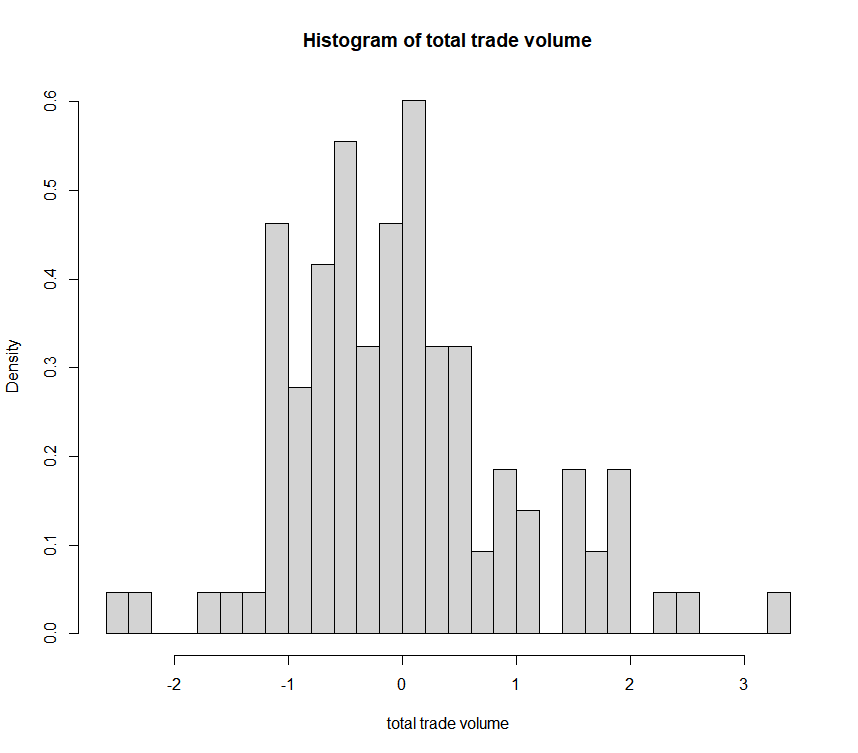
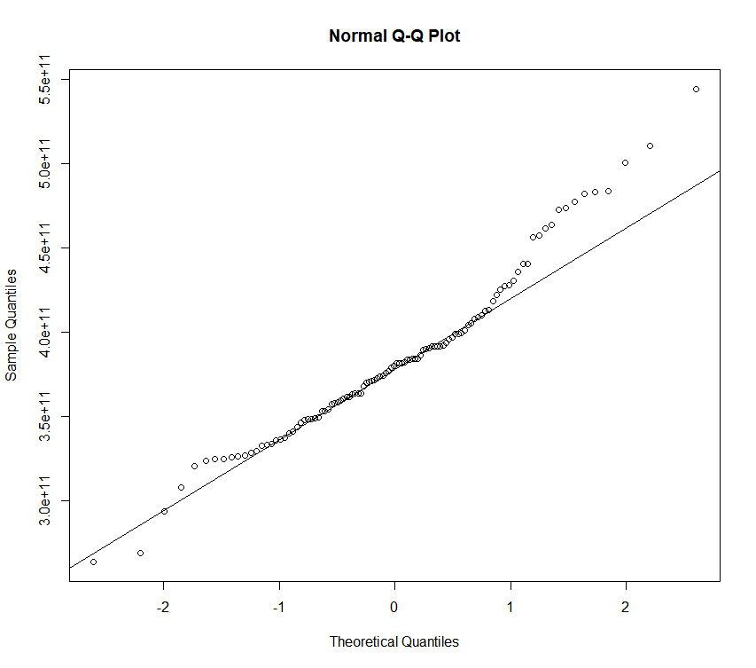
Figure 1: Histogram (a) and normal Q-Q plot (b) of total trade volume of 15 commodities between 22 countries at each time point.

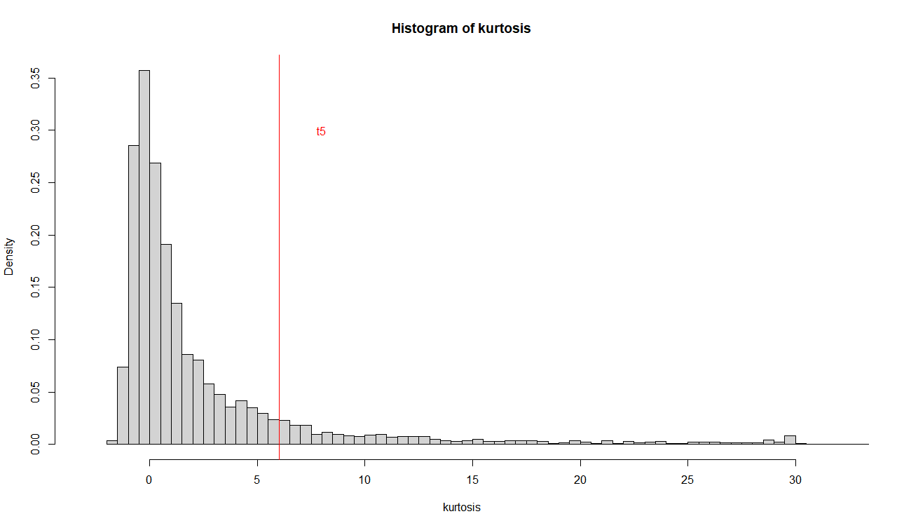
Figure 2: Histogram of the sample kurtosis for $22\times 22\times 15$ trade volumes and the red dashed line is the theoretical kurtosis of $t_{5}$ distribution.

Figure 1 and 1 show the histogram and normal Q-Q plot of the total trade volume at each time point $t$ by adding the volume of trade between 22 countries for 15 commodities, respectively. It can be seen that the total trade volume deviates from the normal distribution and is skewed to the right. Figure 2 shows the histogram of sample kurtosis of $22\times 22\times 15$ variables with respect to the trade volume of 15 commodities among 22 countries, where the red vertical line represents the theoretical kurtosis of the $t_{5}$ distribution. It suggests that this dataset has heavy tails.

In order to assess the goodness of fit, we use the relative Mean Squared Error (MSE) defined as

$$\mathrm{MSE}=\frac{\sum_{t=1}^{T}\|\mathcal{X}_{t}-\widehat{{\mathcal{S}}}_{t}\|_{F}^{2}}{\sum_{t=1}^{T}\|\mathcal{X}_{t}\|_{F}^{2}},$$

where $\widehat{{\mathcal{S}}}_{t}=\widehat{\mathcal{F}}_{t}\times_{1}\widehat{\mathbf{A}}_{1}\times_{2}\widehat{\mathbf{A}}_{2}\times_{3}\widehat{\mathbf{A}}_{3}$ is the estimated three-month average import-export factor driven tensor component of the data tensor at $t$-th moment. When the MSE is small, this means that there is strong evidence of comovements among the variables, thus indicating that the factor model is an adequate representation of the data. Table 5 shows the MSE of the three-month moving average estimated by different methods given different combinations of factor numbers. Specifically, we compare our RTFA method with the following estimators: Initial Estimator (IE) and the Projection Estimator (PE) by Barigozzi et al. (2022b), Iterative Projected mode-wise PCA estimation (IPmoPCA) by Zhang et al. (2022), and the Time series Inner-Product Unfolding Procedure (TIPUP) with their iteration versions (iTIPUP) by Chen et al. (2022b). It can be seen that the estimation accuracy of the non-iterative method is inferior to that of the corresponding iterative method, and the best one is the proposed RTFA method.

Table 5: The MSE for the three-month moving average data. $r_{1}=r_{2}=r_{3}=r$ is the number of factors.

r	IE	PE	IPmoPCA	RTFA	TIPUP	iTIPUP
4	0.005052	0.003243	0.002973	0.002958	0.005055	0.002991
5	0.004675	0.003061	0.002446	0.002403	0.004676	0.002445
6	0.003885	0.002028	0.002025	0.001999	0.003734	0.002022

Table 6: The averaged MSE of rolling validation for the three-month moving average data. $12n$ is the sample size of the training set. $r_{1}=r_{2}=r_{3}=r$ is the number of factors.

$n$	$r$	IE	PE	IPmoPCA	RTFA	TIPUP	iTIPUP
1	4	0.305648	0.234050	0.207419	0.207050	0.306730	0.218064
2	4	0.306979	0.232142	0.190624	0.190185	0.307584	0.192854
3	4	0.307025	0.217422	0.186855	0.186556	0.307332	0.187705
1	5	0.261384	0.176364	0.172087	0.172043	0.258143	0.172437
2	5	0.260488	0.177568	0.167676	0.167616	0.258174	0.166238
3	5	0.259934	0.166453	0.149322	0.149246	0.258230	0.149851
1	6	0.164834	0.114599	0.114138	0.113976	0.159747	0.114077
2	6	0.148967	0.111139	0.110729	0.110743	0.145592	0.110896
3	6	0.163283	0.108324	0.108366	0.108390	0.159581	0.108561

Then we use a rolling-validation procedure as in Wang et al. (2019) to futher compare these methods. For each year $t$ from 2017 to 2022, we repeatedly use the $n$ (bandwidth) year observations prior to $t$ to fit the tensor factor model and estimate the loading matrices. The estimated loading matrices are then used to estimate the factor tensors and the corresponding residuals of the 12 months in the current year. Specifically, let $\mathcal{X}_{t}^{i}$ be the observed import-export tensor of month $i$ in year $t$ and $\widehat{{\mathcal{S}}}_{t}^{i}=\widehat{\mathcal{F}}_{t}^{i}\times_{1}\widehat{\mathbf{A}}_{1}^{i,n}\times_{2}\widehat{\mathbf{A}}_{2}^{i,n}\times_{3}\widehat{\mathbf{A}}_{3}^{i,n}$, where $\{\mathbf{A}_{k}^{i,n}\}_{k=1}^{K}$ are the loading matrices estimated based on $n$ years of observations prior to month $i$ in year $t$, and further define

$$\mathrm{MSE}_{t}=\frac{\sum_{i=1}^{12}\left\|\mathcal{X}_{t}^{i}-\widehat{{\mathcal{S}}}_{t}^{i}\right\|_{F}^{2}}{\sum_{i=1}^{12}\left\|\mathcal{X}_{t}^{i}\right\|_{F}^{2}}$$

as the mean squared error. Table 6 compares the mean values of MSE of various estimation methods for different combinations of bandwidth $n$ and factor number $r_{1}=r_{2}=r_{3}=r$. The estimation errors of IPmoPCA, RTFA and iTIPUP methods are very close together, and the results in Table 6 show that these three methods perform better than the other methods. It is worth noting that our proposed RTFA performs better than the other methods in almost all considered settings. This indicates that RTFA is particularly suitable for capturing comovements in this heavy-tailed data.

Table 7: Estimated loading matrix $\widehat{\mathbf{A}}_{3}^{\top}$ for the commodity mode.

Factor	Animal	Vegetable	Food	Mineral	Chemicals	Plastics	Leather	Wood	Textiles	Footwear	Stone	Metals	Machinery	Transport	Misc
1	0	3	-1	0	-1	1	0	-3	1	0	1	0	29	0	6
2	0	0	0	30	1	-1	0	3	-1	0	0	1	0	0	2
3	0	-3	1	-2	29	3	1	0	0	0	-2	3	0	0	6
4	0	-1	4	0	0	-2	0	2	0	0	-1	1	0	30	2
5	6	6	6	0	-2	19	0	6	4	1	0	17	1	0	-9
6	1	4	4	-1	2	-4	0	5	1	1	29	1	-1	0	2

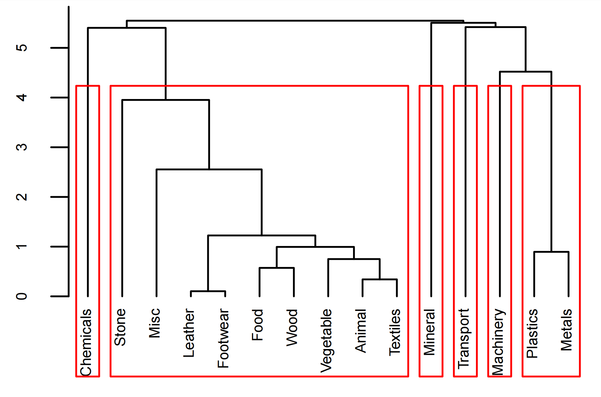
Figure 3: Clustering of product categories by their loading coefficients.

We then use RTFA to further analyze the export-import tensor time series data and, hereafter, we set $r_{1}=r_{2}=4,\leavevmode\nobreak\ r_{3}=6$ as in Chen et al. (2022b).

Table 7 shows the estimated loadings $\widehat{\mathbf{A}}_{3}^{\top}$ for the commodity mode obtained using the RTFA procedure. For better interpretation, the loading matrix is rotated using the varimax procedure (see e.g. Mardia et al., 1979, Chapter 9.6) and all numbers are multiplied by 30 and then truncated to integers for clearer viewing The sign of each row of $\widehat{\mathbf{A}}_{3}^{\top}$ (column of $\widehat{\mathbf{A}}_{3}$) is set in such a way that the largest entry (in boldface) is positive. It can be seen from Table 7 that there is a group structure of these six category factors. Hence, each factor is represents a “condensed product group” in Chen et al. (2022b). Factor 1, 2, 3, 4 and 6 can be interpreted as Machinery & Electrical factor, Mineral Products factor, Chemicals & Allied Industries factor, Transportation factor and Stone & Glass factor, because these factors are mainly loaded on these commodity categories. Factor 5 can be viewed as a mixing factor, with Plastics & Rubbers and Metals as main load. The clustering of the product categories according to their loading vectors, the 15 columns of $\widehat{\mathbf{A}}_{3}^{\top}$ each of dimension 6, is shown in Figure 3. The distance between two product categories $i$ and $j$ is defined by Euclidean distance, which is $d_{ij}^{2}=\sum_{k=1}^{6}\left((\widehat{\mathbf{A}}_{3})_{ki}-(\widehat{\mathbf{A}}_{3})_{kj}\right)^{2}/\widehat{\operatorname{Var}}(\widehat{\mathbf{A}}_{3})_{k\cdot}=d_{ji}^{2}$, where $\widehat{\operatorname{Var}}(\widehat{\mathbf{A}}_{3})_{k\cdot}$ is the sample variance of the $k$th row of $\widehat{\mathbf{A}}_{3}^{\top}$. In this study, we adopt the “complete linkage method” (see e.g. Hubert, 1974) for clustering in this study.

As pointed out by Chen et al. (2022b), each frontal slice of the factor $\mathcal{F}_{t}$, which is equal to $\mathcal{G}_{\cdot,\cdot,i_{3},t}$, can be regarded as the trade of $i_{3}$ commodity types between several virtual export hubs and virtual import hubs. Each commodity transaction can be seen as first the product is transported from the exporting country to an export hub, then exported from the export hub to an import hub, and finally reaches the importing country from the import hub. Each row of $\mathcal{G}_{\cdot,\cdot,i_{3},t}$ represents an exit hub and each column represents an import hub. The corresponding estimated loading matrices $\widehat{\mathbf{A}}_{1}^{\top}$ and $\widehat{\mathbf{A}}_{2}^{\top}$ computed by the RTFA method, can reflect the trading activities of each country through each export hub and import hub, respectively. They are reported in Tables 8 and 9, respectively. The scale and sign of the entries of this tables is set in the same way as for Table 7 above.

Table 8: Estimated loading matrix $\widehat{\mathbf{A}}_{1}^{\top}$ for the export mode.

Factor	BE	BU	CA	DK	FI	FR	DE	GR	HU	IS	IR	IT	MX	NO	PO	PT	ES	SE	CH	ER	US	GB
1	-1	0	0	0	0	1	3	0	0	0	-3	1	30	0	0	0	-1	0	-1	0	0	1
2	0	0	0	0	0	0	-2	0	1	0	-2	1	0	0	1	0	0	0	0	0	30	0
3	1	0	30	0	0	0	-1	0	0	0	2	0	0	1	0	0	0	0	1	0	0	1
4	7	0	0	2	1	9	22	0	2	0	9	8	-2	1	4	1	6	2	7	2	1	6

Table 9: Estimated loading matrix $\widehat{\mathbf{A}}_{2}^{\top}$ for the import fiber.

Factor	BE	BU	CA	DK	FI	FR	DE	GR	HU	IS	IR	IT	MX	NO	PO	PT	ES	SE	CH	ER	US	GB
1	0	0	0	0	0	0	0	0	0	0	0	0	0	0	0	0	0	0	0	0	30	0
2	2	0	28	0	0	3	7	0	0	0	4	1	-2	1	1	0	1	0	5	1	0	1
3	7	1	-7	2	1	14	10	1	4	0	1	11	1	1	6	2	7	4	6	3	0	14
4	-2	0	3	0	0	-1	1	0	0	0	-2	-2	29	0	-1	0	0	0	-5	0	0	4

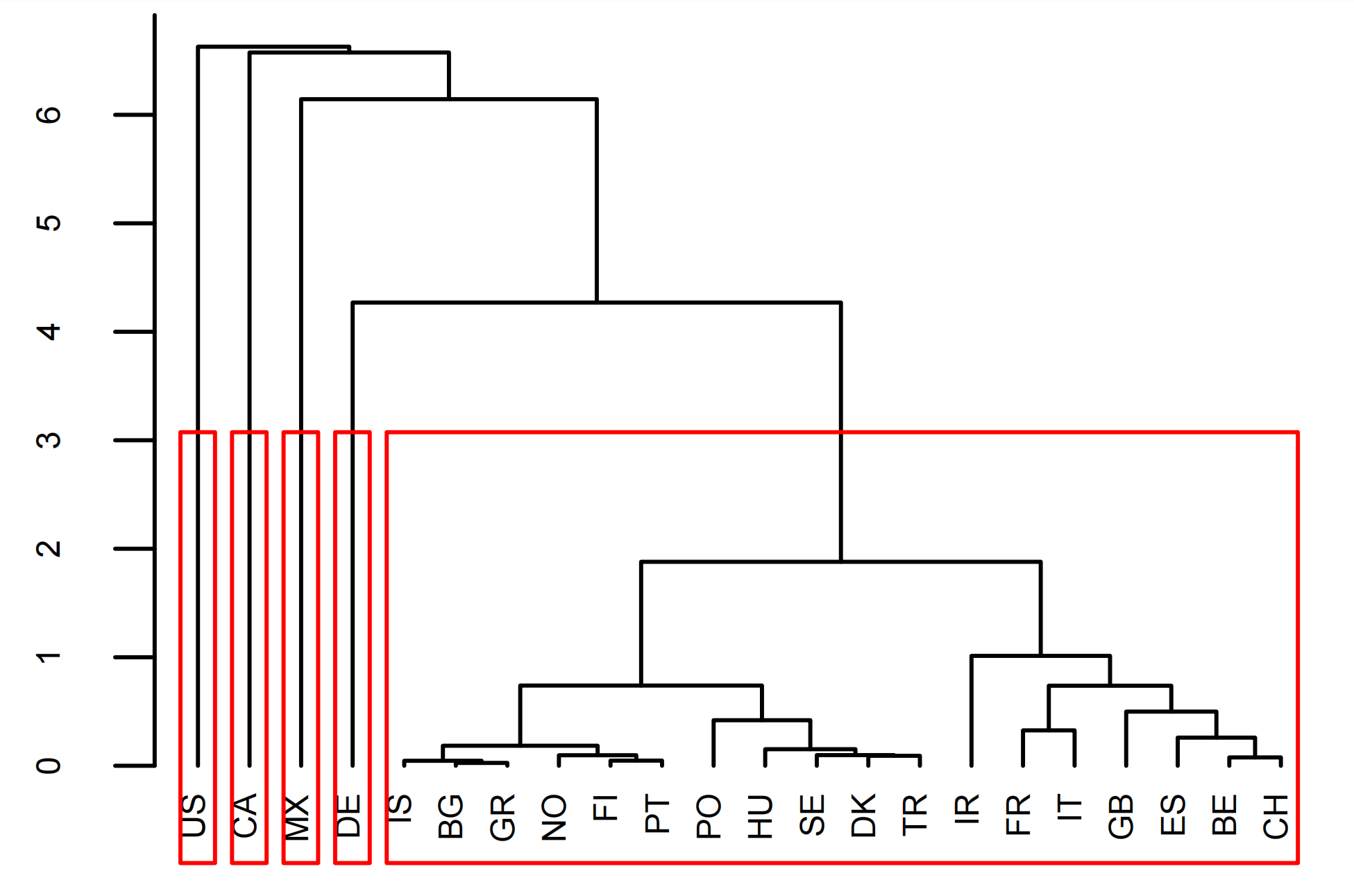
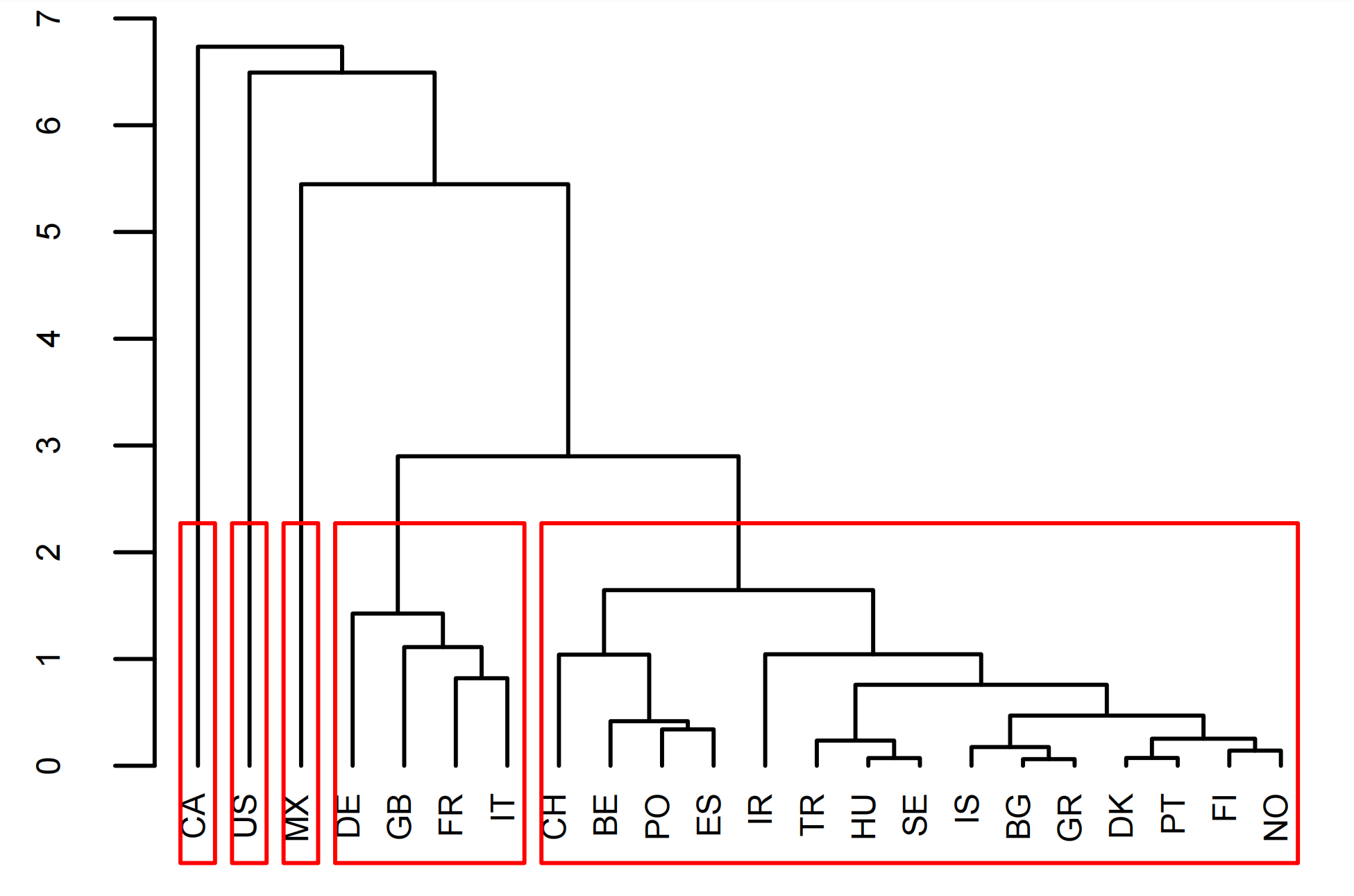
Figure 4: Clustering of countries by their export (a) and import (b) loading coefficients.

The loading matrices are also rotated via varimax procedure.Mexico, the United States of America and Canada heavily load on virtual export hubs E1, E2 and E3, respectively. European countries mainly load on export hub E4, and Germany occupies an important position. The United States of America, Mexico and Canda heavily load on virtual import hubs I1, I2 and I4. European countries mainly load on import hub I3, led by France and Britain. Figures 4 and 4 show the clustering of loadings for $\widehat{\mathbf{A}}_{1}$ and $\widehat{\mathbf{A}}_{2}$ respectively.

For exporting activities, the three countries in the America are very different from the European countries, and Germany is divided into a separate group and other European countries into another. For importing activities, the three North American countries still differ markedly from Europe. Germany, the United Kingdom, France and Italy are grouped into one cluster, and the other countries are grouped into another.

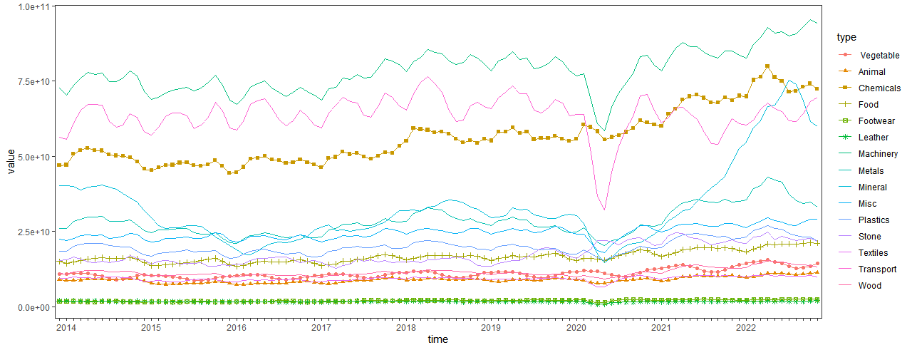
Figure 5: Total trade volume of each commodity between 22 countries at each moment.

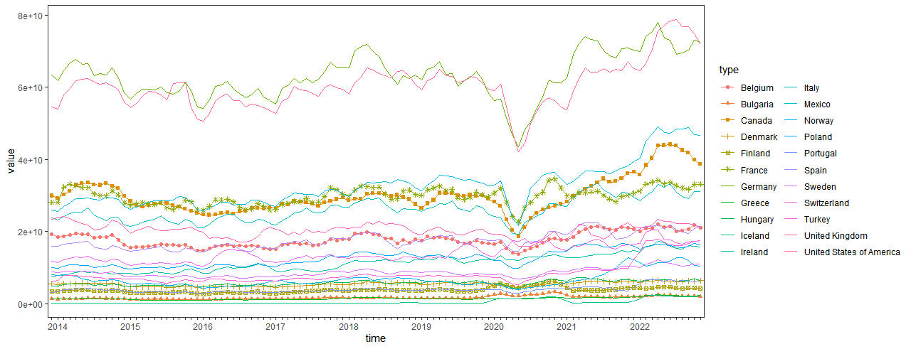
Figure 6: Each country’s total export trade with 21 other countries for 15 commodities at each moment.

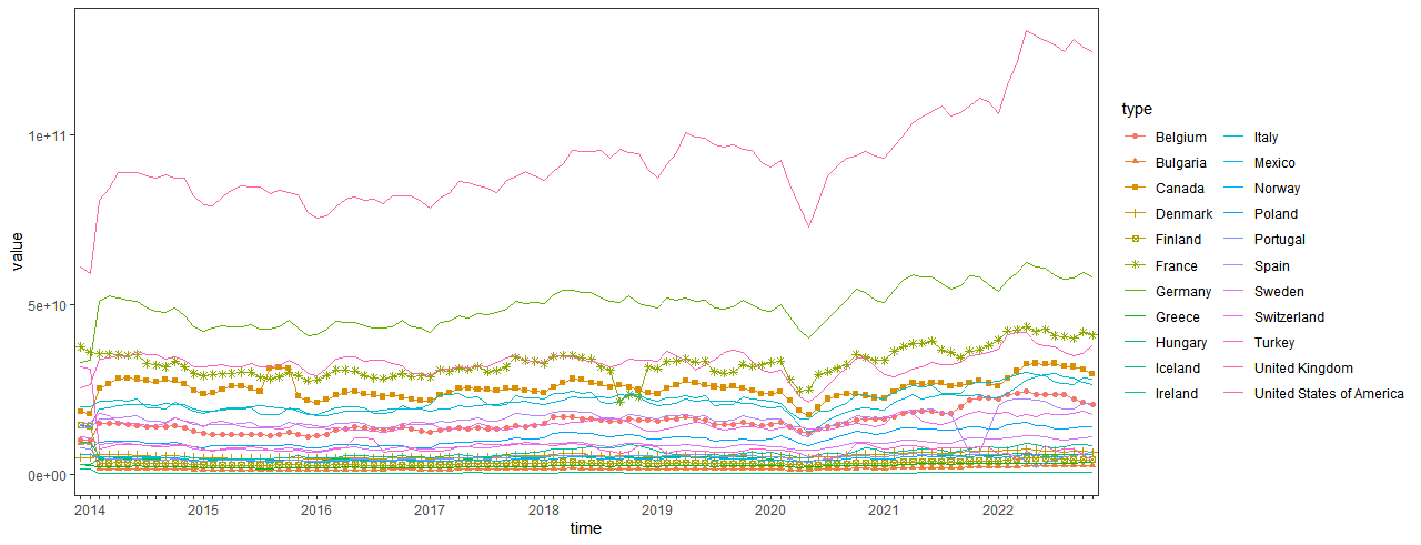
Figure 7: Each country’s total import trade with 21 other countries for 15 commodities at each moment.

Figure 5 shows the total volume of trade between the 22 countries for each commodity at each time. We can see that the product categories with the largest volume of import-export are Machinery & Electrical, Transportation and Chemicals & Allied Industries. Each country’s total export trade volumes and import trade volumes with 21 other countries for 15 commodities at each moment are shown in Figures 6 and 7. The largest importers are Germany, the United States of America, followed by Mexico, Canada, France and Italy. The largest exporters are the United States of America, Germany, followed by France and the United Kingdom. All three charts show larger fluctuations in 2020, which is understandable because of COVID-19. And around 2021, the potential factor model of the data may change. We will analyze this change by dividing the data into two groups for 2014-2019 and 2020-2022, written as period $\mathcal{I}$ and $\mathcal{I}\mathcal{I}$. Although period $\mathcal{I}\mathcal{I}$ is relatively short we recall that when estimating the loadings the effective sample size is $Tp_{-k}$ which is instead quite large.

Table 10: Estimated loadings matrix $\widehat{\mathbf{A}}_{3}^{\top}$ for the commodity mode in periods $\mathcal{I}$ and $\mathcal{I}\mathcal{I}$.

Period	Factor	Animal	Vegetable	Food	Mineral	Chemicals	Plastics	Leather	Wood	Textiles	Footwear	Stone	Metals	Machinery	Transport	Misc
$\mathcal{I}$	1	0	2	-1	0	-1	1	0	-2	1	0	0	0	29	1	6
	2	0	1	-1	30	1	-1	0	3	-1	0	1	1	0	0	1
	3	0	-3	1	-1	29	2	0	1	0	0	0	2	0	0	7
	4	0	0	4	0	0	-2	0	2	0	0	-1	1	0	29	2
	5	6	6	6	0	0	20	0	6	5	1	1	16	1	0	-9
	6	2	4	1	-1	0	-4	0	3	1	1	29	0	0	0	1
$\mathcal{I}\mathcal{I}$	1	-1	3	0	0	1	2	0	6	0	0	0	-1	29	2	5
	2	0	1	0	30	2	-1	0	2	-1	0	0	1	0	-1	1
	3	0	-2	1	-3	29	1	1	1	1	0	0	1	-1	3	6
	4	6	6	6	0	0	19	0	7	4	0	0	17	2	-1	-8
	5	1	0	4	0	-4	-4	0	7	0	0	0	2	0	28	3
	6	1	-1	1	0	0	-1	0	5	1	0	29	0	1	-2	2

Table 11: Estimated loadings matrix $\widehat{\mathbf{A}}_{1}^{\top}$ for the export mode in periods $\mathcal{I}$ and $\mathcal{I}\mathcal{I}$.

Period	Factor	BE	BU	CA	DK	FI	FR	DE	GR	HU	IS	IR	IT	MX	NO	PO	PT	ES	SE	CH	ER	US	GB
$\mathcal{I}$	1	-2	0	1	0	0	0	3	0	0	0	-2	1	30	0	0	0	-1	0	-1	0	0	1
	2	0	0	-1	0	0	0	-2	0	1	0	-1	1	0	0	1	0	0	0	0	0	30	0
	3	1	0	30	0	0	0	0	0	0	0	2	0	-1	1	0	0	0	0	1	0	1	1
	4	6	0	-1	2	1	9	23	0	2	0	7	7	-1	1	4	1	6	2	6	2	1	6
$\mathcal{I}\mathcal{I}$	-1	-1	0	0	0	0	0	3	0	0	0	-3	1	30	0	0	0	0	0	-1	0	0	1
	2	0	0	0	0	0	1	-1	0	1	0	-2	1	-1	1	1	0	1	0	0	0	30	1
	-3	0	0	30	0	0	0	-1	0	0	0	1	0	0	0	-1	0	0	0	0	0	0	1
	-4	7	0	0	2	1	8	19	0	2	0	13	8	-1	1	4	1	5	2	9	2	1	5

Table 12: Estimated loadings matrix $\widehat{\mathbf{A}}_{2}^{\top}$ for the import mode in periods $\mathcal{I}$ and $\mathcal{I}\mathcal{I}$.

Period	Factor	BE	BU	CA	DK	FI	FR	DE	GR	HU	IS	IR	IT	MX	NO	PO	PT	ES	SE	CH	ER	US	GB
$\mathcal{I}$	1	0	0	0	0	0	0	0	0	0	0	0	0	0	0	0	0	0	0	0	0	30	0
	2	-1	0	3	0	0	1	3	0	0	0	-3	-1	29	0	-1	0	-1	0	-4	0	0	4
	3	7	1	-5	2	1	15	10	1	4	0	1	10	0	1	6	2	8	4	7	4	0	15
	4	1	0	29	0	0	2	5	0	-1	0	5	1	-2	1	0	0	1	0	3	1	0	1
$\mathcal{I}\mathcal{I}$	1	0	0	1	0	0	0	0	0	0	0	0	0	0	0	0	0	0	0	0	0	30	0
	2	-1	0	21	0	0	0	6	0	-1	0	2	-1	20	0	-1	0	1	0	-1	0	0	0
	3	11	1	-1	3	1	16	14	1	4	0	2	12	-2	1	7	2	7	4	8	3	0	1
	4	-2	0	-1	0	0	-1	-1	0	0	0	-1	-1	2	0	0	0	0	0	2	0	0	30

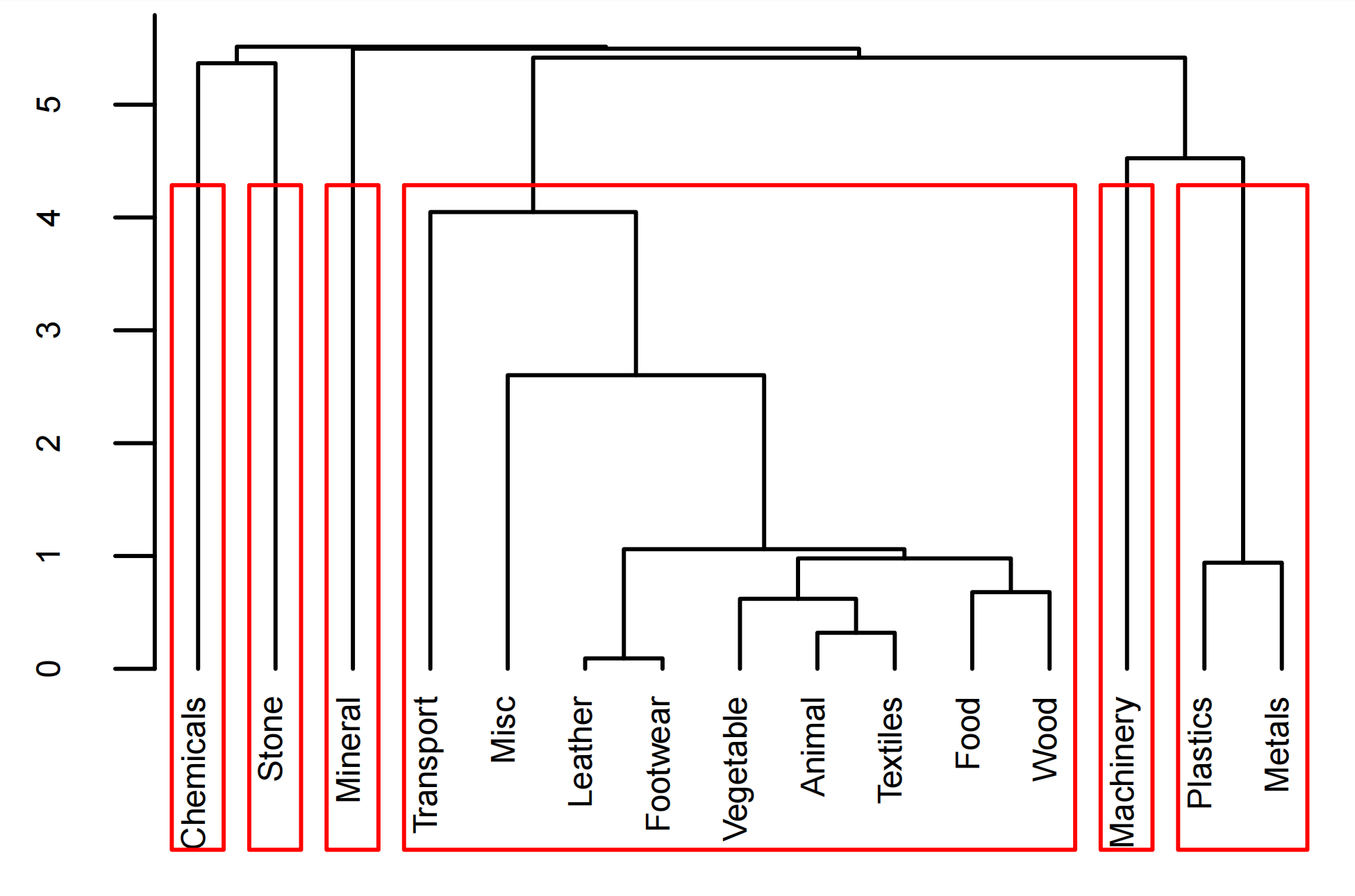
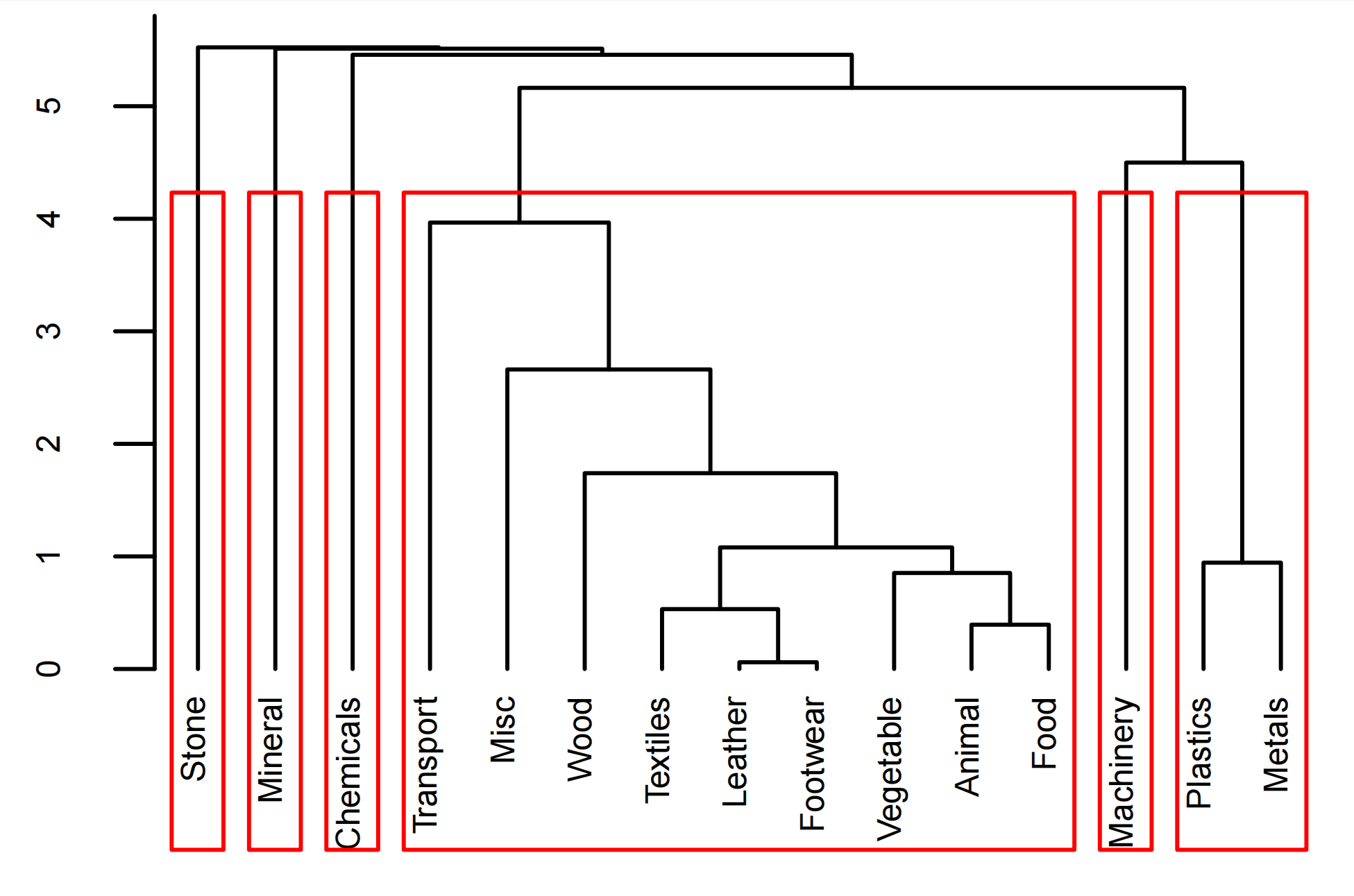
Figure 8: Clustering of product categories by their loading coefficients in periods $\mathcal{I}$ (a) and $\mathcal{I}\mathcal{I}$ (b).

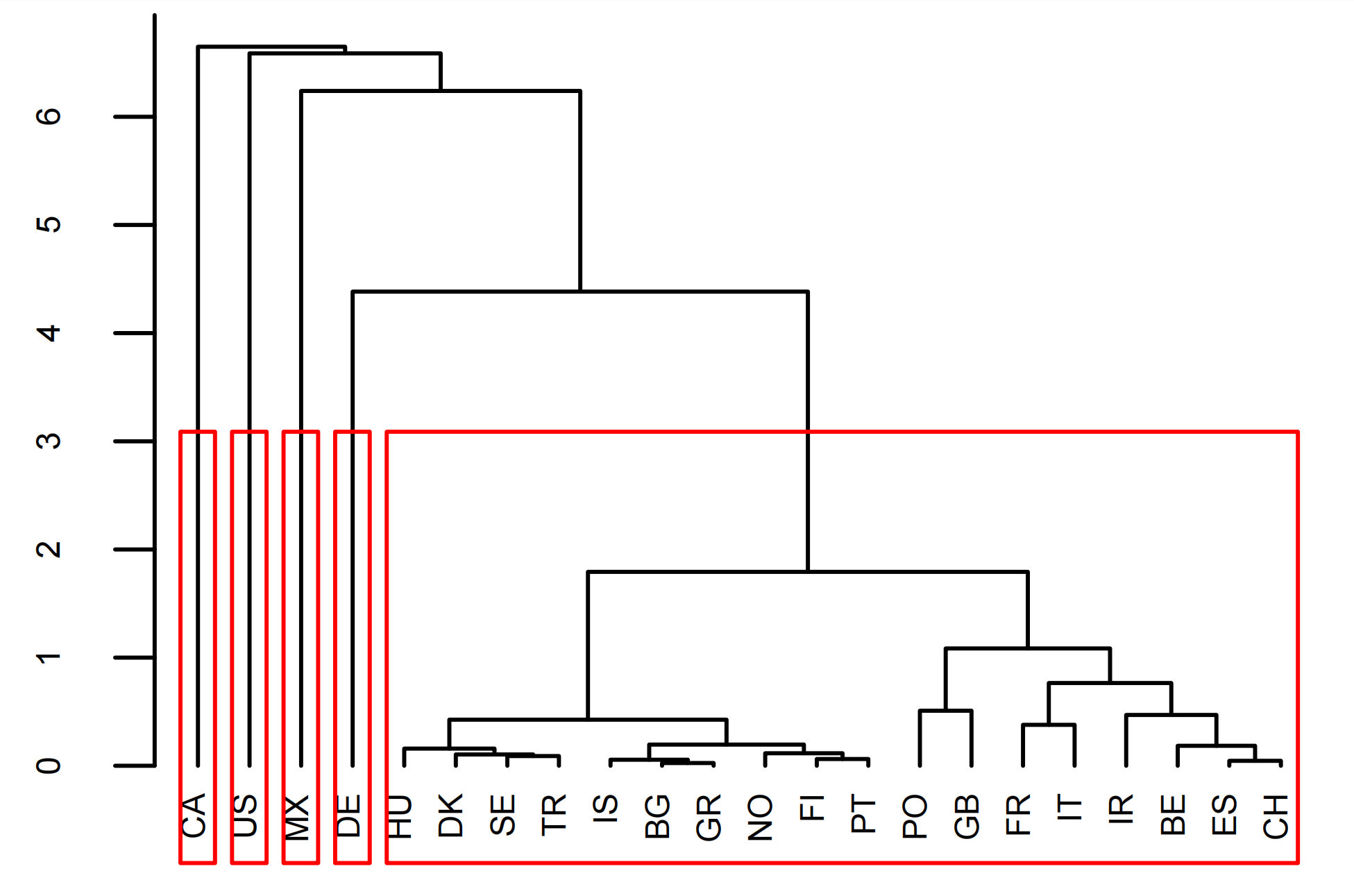
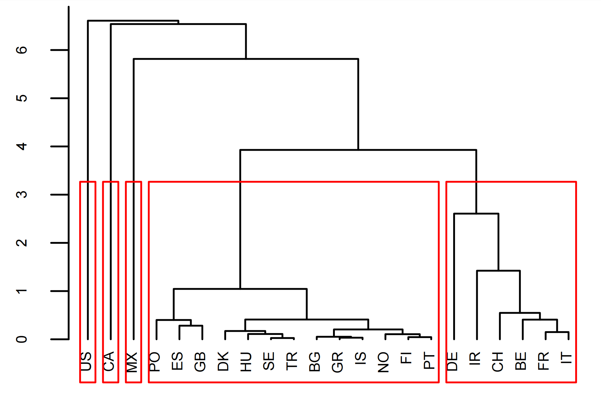
Figure 9: Clustering of countries by their export loading coefficients in periods $\mathcal{I}$ (a) and $\mathcal{I}\mathcal{I}$ (b).

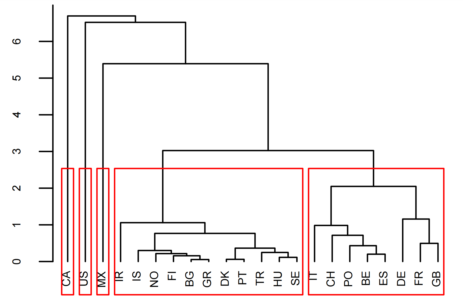
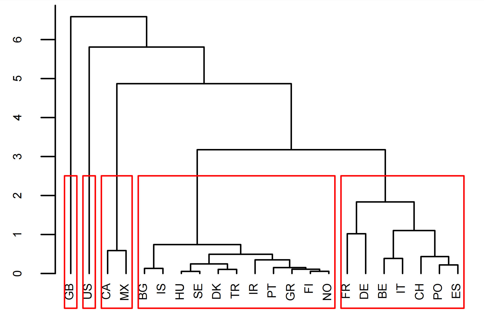
Figure 10: Clustering of countries by their import loading coefficients in periods $\mathcal{I}$ (a) and $\mathcal{I}\mathcal{I}$ (b).

Tables 10, 11 and 12 show the estimated loading matrices $\widehat{\mathbf{A}}_{3}$, $\widehat{\mathbf{A}}_{1}$, and $\widehat{\mathbf{A}}_{2}$, respectively, of import-export data for two periods, and their corresponding clustering results is shown in Figures 8 and 8, 9 and 9, and 10 and 10, respectively.

For product categories and exporting countries, the estimation of loading matrices in the two periods are very similar. The clustering results also illustrate this point. It is suggested that there are some difference in estimation of $\mathbf{A}_{2}$. In period $\mathcal{I}$, the United States of America, Mexico and Canada heavily load on virtual import hubs I1, I2 and I3, European countries mainly load on import hub I3, dominated by France and the United Kingdom. In period $\mathcal{I}\mathcal{I}$, the United States of America and the United Kingdom heavily load on virtual import hubs I1 and I4, American countries Canada and Mexico mainly load on import hub I2 while hub I3 is mainly loaded by European countries France and Germany.

6 Conclusion

In this paper, we study inference in the context of a factor model for tensor-valued time series, from the perspective of both Least Squares and Huber Loss. As far as the former is concerned, we investigate the consistency of the estimated common factors and loadings space when using estimators based on minimising quadratic loss functions. Building on the observation that such loss functions are adequate only if sufficiently many moments exist, we extend our results to the case of heavy-tailed distributions by considering estimators based on minimising the Huber loss function, which uses an $L_{1}$-norm weight on outliers. We show that such class of estimators is robust to the presence of heavy tails, even when only the second moment of the data exists. We also propose a modified version of the eigenvalue-ratio principle to estimate the dimensions of the factors tensor, and show the consistency of such estimators without any condition on the relative rates of divergence of the dimensions $p_{1}$, …, $p_{K}$ and $T$. Extensive numerical results show the proposed methods performs better than the state-of-the-art ones, and that our proposed methodology is particularly effective when data exhibit heavy tails. In the paper, we also show that the iterative version of our estimators performs very well; deriving theoretical guarantees for the estimators in the solution path of the iterative algorithm is a very interesting, and challenging, topic, which is currently under investigation by the authors.

Appendix A Preliminary lemmas

Henceforth, we use the following notation. Recall that, by (3.1)

$$L=\min\left\{p,Tp_{-1},...,Tp_{-K}\right\}.$$

Further, let $\leavevmode\nobreak\ r=r_{1}\cdots r_{k}$; we define

$$M=\sum_{k=1}^{K}p_{k}r_{k}+Tr,$$ (A.1)

as the total number of parameters to be estimated. We define the function

$$\mathbb{M}(\theta)=\frac{1}{Tp}\sum_{t=1}^{T}\sum_{i_{1}=1}^{p_{1}}\cdots\sum_{i_{K}=1}^{p_{K}}\left(x_{t,i_{1},\cdots,i_{K}}-\mathcal{F}_{t}\times_{k=1}^{K}\bm{a}_{k,i_{k}}^{\top}\right)^{2}=\frac{1}{Tp}\sum_{t=1}^{T}\left\|\mathcal{X}_{t}-\mathcal{F}_{t}\times_{k=1}^{K}\mathbf{A}_{k}\right\|_{F}^{2};$$ (A.2)

it can be readily seen that minimizing $\mathbb{M}(\theta)$ is equivalent to minimizing the Least Squares loss $L_{1}\left(\mathbf{A}_{1},\cdots,\mathbf{A}_{K},\mathcal{F}_{t}\right)$, whence $\widehat{\theta}$ is (alternatively) defined as

$$\widehat{\theta}=\left(\widehat{\mathbf{A}}_{1},\cdots,\widehat{\mathbf{A}}_{K},\widehat{\mathcal{F}}_{1},\cdots,\widehat{\mathcal{F}}_{T},\right)=\underset{\theta\in\Theta}{\arg\min}\mathbb{M}(\theta).$$

In addition to $\mathbb{M}(\theta)$, we introduce the quantities

$$\mathbb{M}^{\ast}\left(\theta\right) = \frac{1}{Tp}\sum_{t=1}^{T}\sum_{i_{1}=1}^{p_{1}}...\sum_{i_{K}=1}^{p_{K}}w\left(\bm{a}_{1,i_{1}},,...,\bm{a}_{K,i_{K}},\mathcal{F}_{t}\right),$$ (A.3)

$$\overline{\mathbb{M}}^{\ast}\left(\theta\right) = \mathbb{E}\left(\mathbb{M}^{\ast}\left(\theta\right)\right)=\frac{1}{Tp}\sum_{t=1}^{T}\sum_{i_{1}=1}^{p_{1}}...\sum_{i_{K}=1}^{p_{K}}\mathbb{E}\left[w\left(\bm{a}_{1,i_{1}},,...,\bm{a}_{K,i_{K}},\mathcal{F}_{t}\right)\right],$$ (A.4)

$$\mathbb{W}\left(\theta\right) = \mathbb{M}^{\ast}\left(\theta\right)-\overline{\mathbb{M}}^{\ast}\left(\theta\right),$$ (A.5)

where we have defined

$$w\left(\bm{a}_{1,i_{1}},\cdots,\mathbf{b}_{K,i_{K}},\mathcal{F}_{t}\right)=\left(x_{t,i_{1},\cdots,i_{K}}-\mathcal{F}_{t}\times_{k=1}^{K}\bm{a}_{k,i_{k}}^{\top}\right)^{2}-\left(x_{t,i_{1},\cdots,i_{K}}-\mathcal{F}_{0t}\times_{k=1}^{K}\bm{a}_{0k,i_{k}}^{\top}\right)^{2}.$$ (A.6)

We will make extensive use of the semimetric

$$d\left(\theta_{a},\theta_{b}\right) = \sqrt{\frac{1}{Tp}\sum_{t=1}^{T}\sum_{i_{1}=1}^{p_{1}}...\sum_{i_{K}=1}^{p_{K}}\left(\mathcal{F}_{at}\times_{k=1}^{K}\bm{a}_{ak,i_{k}}^{\top}-\mathcal{F}_{bt}\times_{k=1}^{K}\bm{a}_{bk,i_{k}}^{\top}\right)^{2}}$$

$$= \sqrt{\frac{1}{Tp}\sum_{t=1}^{T}\left\|\mathcal{F}_{at}\times_{k=1}^{K}\bm{A}_{ak}-\mathcal{F}_{bt}\times_{k=1}^{K}\bm{A}_{bk}\right\|_{F}^{2}.}$$

Further, we let $C(\cdot,g,\mathcal{G})$ and $D(\cdot,g,\mathcal{G})$ be the covering number and the packing number, respectively, of space $\mathcal{G}$ equipped with the semimetric $g$. Throughout the proof, we denote positive, finite constants as $c_{0}$, $c_{1}$, … and their value may change from line to line.

For a random variable $X$ and a non-decreasing, convex function $\psi$ such that $\psi\left(0\right)=0$, we define the Orlicz norm as $\|X\|_{\psi}=\inf\{C>0:\mathbb{E}\psi(|X|/C)\leq 1\}$. In particular, based on the function $y=\psi^{2}\left(x\right)$, we use the notation

$$\|X\|_{\psi^{2}}=\inf\{C>0:\mathbb{E}\exp\left(\frac{\left|X\right|}{C}\right)^{2}\leq 1\}.$$

Lemma A.1.

We assume that Assumptions 1-3 hold. Then, as $\min\left\{p_{1},...,p_{K},T\right\}\rightarrow\infty$, it holds that

$$d\left(\widehat{\theta},\theta_{0}\right)=o_{P}\left(1\right).$$

Proof.

We begin by noting that, for any $\mathbf{A}_{k}$, $1\leq k\leq K$, and for any $\mathcal{F}_{t}\in\mathcal{F}$, it holds that, using Assumptions 2 and 3

$$\mathbb{E}\left[w\left(\bm{a}_{1,i_{1}},,...,\bm{a}_{K,i_{K}},\mathcal{F}_{t}\right)\right]$$

$$= \mathbb{E}\left[\left(x_{t,i_{1},...,i_{K}}-\mathcal{F}_{t}\times_{k=1}^{K}\bm{a}_{k,i_{k}}^{\top}\right)^{2}-\left(x_{t,i_{1},...,i_{K}}-\mathcal{F}_{0t}\times_{k=1}^{K}\bm{a}_{0k,i_{k}}^{\top}\right)^{2}\right]$$

$$= \mathbb{E}\left(\mathcal{F}_{t}\times_{k=1}^{K}\bm{a}_{k,i_{k}}^{\top}-\mathcal{F}_{0t}\times_{k=1}^{K}\bm{a}_{0k,i_{k}}^{\top}\right)\left(\mathcal{F}_{t}\times_{k=1}^{K}\bm{a}_{k,i_{k}}^{\top}-\mathcal{F}_{0t}\times_{k=1}^{K}\bm{a}_{0k,i_{k}}^{\top}+2e_{t,i_{1},...,i_{K}}\right)$$

$$= \left(\mathcal{F}_{t}\times_{k=1}^{K}\bm{a}_{k,i_{k}}^{\top}-\mathcal{F}_{0t}\times_{k=1}^{K}\bm{a}_{0k,i_{k}}^{\top}\right)^{2}.$$

Then, recalling (A.4), for any $\theta\in\Theta$ it follows that

$$\overline{\mathbb{M}}^{\ast}(\theta)=d^{2}\left(\theta,\theta_{0}\right).$$

By definition, it holds that

$$\mathbb{M}^{\ast}(\widehat{\theta})=\mathbb{M}(\widehat{\theta})-\mathbb{M}\left(\theta_{0}\right)\leq 0,$$

and therefore, using the definition of (A.5)

$$\mathbb{W}(\widehat{\theta})+\overline{\mathbb{M}}^{\ast}(\widehat{\theta})=\mathbb{M}^{\ast}(\widehat{\theta})\leq 0.$$

Hence, it ultimately follows that

$$0\leq d^{2}\left(\widehat{\theta},\theta_{0}\right)=\overline{\mathbb{M}}^{\ast}(\widehat{\theta})\leq\sup_{\theta\in\Theta}|\mathbb{W}(\theta)|,$$

which entails that it is sufficient to prove that

$$\sup_{\theta\in\Theta}|\mathbb{W}(\theta)|=o_{P}(1).$$ (A.9)

For any $\theta\in\Theta$, define $\theta^{\ast}=\left(\mathbf{A}_{1}^{\ast},\cdots,\mathbf{A}_{K}^{\ast},\mathcal{F}_{1}^{\ast},\cdots,\mathcal{F}_{T}^{\ast}\right)$, where, for all $1\leq k\leq K$

$$\bm{a}_{k,i_{k}}^{\ast}=\left\{\bm{a}_{k,(i)}:i\leq J_{k},\left\|\bm{a}_{k,(i)}-\bm{a}_{k,i_{k}}\right\|_{2}\leq\epsilon/C_{1}\right\},$$ (A.10)

and

$$\mathcal{F}_{t}^{\ast}=\left\{\mathcal{F}_{(h)}:h\leq J_{H},\left\|\mathcal{F}_{(h)}-\mathcal{F}_{t}\right\|_{F}\leq\epsilon/C_{1}\right\}.$$ (A.11)

Hence, using the fact that $\mathbb{W}(\theta)=\mathbb{W}\left(\theta^{\ast}\right)+\mathbb{W}(\theta)-\mathbb{W}\left(\theta^{\ast}\right)$, (A.9) follows if we show that

$$\sup_{\theta\in\Theta}|\mathbb{W}(\theta)-\mathbb{W}\left(\theta^{\ast}\right)| = o_{P}(1),$$ (A.12)

$$\sup_{\theta\in\Theta}|\mathbb{W}(\theta^{\ast})| = o_{P}(1).$$ (A.13)

We begin with (A.12). Choose $C_{1}$ large enough such that $\left\|\bm{a}_{0k,i_{k}}\right\|_{2}$, $\left\|\mathcal{F}_{0t}\right\|_{F}$, $\left\|\bm{a}_{k,i_{k}}\right\|_{2}$, and $\left\|\mathcal{F}_{t}\right\|_{F}$ are all $\leq C_{1}$ for all $i_{1},\cdots,i_{K},t$ and $1\leq k\leq K$. Let $B_{i}(C_{1})$ denote a Euclidean ball in $\mathbb{R}^{i}$ with radius $K$, for all $i=r_{1},\cdots,r_{K}$; and let $B_{r_{1}\times r_{2}\times\cdots\times r_{K}}(C_{1})$ denote a Euclidean ball in $\mathbb{R}^{r_{1}\times\cdots\times r_{K}}$ with radius $C_{1}$. For any $\epsilon>0$, let $\mathbf{a}_{k,(1)},\cdots,\mathbf{a}_{k,\left(J_{k}\right)}$ be the maximal set of points in $B_{r_{k}}(C_{1})$ such that $\left\|\mathbf{a}_{k,(i)}-\mathbf{a}_{k,(h)}\right\|_{2}>\epsilon/C_{1}$, $\forall i\neq h$; and let $\mathcal{F}_{(1)},\cdots,\mathcal{F}_{\left(H\right)}$ be the maximal set of points in $B_{r_{1}\times\cdots\times r_{K}}(C_{1})$ such that $\left\|\mathcal{F}_{(t)}-\mathcal{F}_{(h)}\right\|_{F}>\epsilon/C$, for $\forall t\neq h$. Then the packing numbers of $B_{r_{k}}(C_{1})$, with $1\leq k\leq K$, and of $B_{r_{1}\times\cdots\times r_{K}}(C_{1})$ are $D_{k}(C_{1}/\epsilon)^{r_{k}}$, and $D_{F}(C_{1}/\epsilon)^{r_{1}\times\cdots\times r_{K}}$, respectively - note that we denote the constants as $D_{k}$, $1\leq k\leq K$, and $D_{F}$ respectively. Note that

$$\mathbb{W}(\theta)-\mathbb{W}\left(\theta^{\ast}\right)$$

$$= \frac{1}{Tp}\sum_{t=1}^{T}\sum_{i_{1}=1}^{p_{1}}...\sum_{i_{K}=1}^{p_{K}}\left[w\left(\bm{a}_{1,i_{1}},,...,\bm{a}_{K,i_{K}},\mathcal{F}_{t}\right)-w\left(\bm{a}_{1,i_{1}}^{\ast},,...,\bm{a}_{K,i_{K}}^{\ast},\mathcal{F}_{t}^{\ast}\right)\right]$$

$$-\frac{1}{Tp}\sum_{t=1}^{T}\sum_{i_{1}=1}^{p_{1}}...\sum_{i_{K}=1}^{p_{K}}\left(\mathbb{E}\left[w\left(\bm{a}_{1,i_{1}},,...,\bm{a}_{K,i_{K}},\mathcal{F}_{t}\right)\right]-\mathbb{E}\left[w\left(\bm{a}_{1,i_{1}}^{\ast},,...,\bm{a}_{K,i_{K}}^{\ast},\mathcal{F}_{t}^{\ast}\right)\right]\right).$$

By standard algebra, it holds that

$$\mathbb{E}\left|w\left(\bm{a}_{1,i_{1}},,...,\bm{a}_{K,i_{K}},\mathcal{F}_{t}\right)-w\left(\bm{a}_{1,i_{1}}^{\ast},,...,\bm{a}_{K,i_{K}}^{\ast},\mathcal{F}_{t}^{\ast}\right)\right|$$

$$= 2\mathbb{E}\left(\left|\mathcal{F}_{t}^{\ast}\times_{k=1}^{K}\bm{a}_{k,i_{k}}^{\ast\top}-\mathcal{F}_{t}\times_{k=1}^{K}\bm{a}_{k,i_{k}}^{\top}\right|\left|x_{t,i_{1},...,i_{K}}-\mathcal{F}_{0t}\times_{k=1}^{K}\bm{a}_{0k,i_{k}}^{\top}\right|\right)$$

$$= 2\mathbb{E}\left(\left|\mathcal{F}_{t}^{\ast}\times_{k=1}^{K}\bm{a}_{k,i_{k}}^{\ast\top}-\mathcal{F}_{t}\times_{k=1}^{K}\bm{a}_{k,i_{k}}^{\top}\right|\left|e_{t,i_{1},...,i_{K}}\right|\right)$$

$$\leq c_{0}\left|\mathcal{F}_{t}^{\ast}\times_{k=1}^{K}\bm{a}_{k,i_{k}}^{\ast\top}-\mathcal{F}_{t}\times_{k=1}^{K}\bm{a}_{k,i_{k}}^{\top}\right|,$$

having used Assumptions 2 and 3. Note now that

$$\left|\mathcal{F}_{t}^{\ast}\times_{k=1}^{K}\bm{a}_{k,i_{k}}^{\ast\top}-\mathcal{F}_{t}\times_{k=1}^{K}\bm{a}_{k,i_{k}}^{\top}\right|$$

$$= \left|\mathcal{F}_{t}\times_{k=1}^{K}\left(\bm{a}_{k,i_{k}}^{\top}-\bm{a}_{k,i_{k}}^{\ast\top}\right)+\left(\mathcal{F}_{t}-\mathcal{F}_{t}^{\ast}\right)\times_{k=1}^{K}\bm{a}_{k,i_{k}}^{\ast\top}\right|$$

$$= \left|\sum_{l=1}^{K}\mathcal{F}_{t}\times_{k=1}^{l-1}\left(\bm{a}_{k,i_{k}}^{\top}-\bm{a}_{k,i_{k}}^{\ast\top}\right)\times_{l}\left(\bm{a}_{l,i_{l}}^{\top}-\bm{a}_{l,i_{l}}^{\ast\top}\right)\times_{k=l+1}^{K}\left(\bm{a}_{k,i_{k}}^{\top}-\bm{a}_{k,i_{k}}^{\ast\top}\right)+\left(\mathcal{F}_{t}-\mathcal{F}_{t}^{\ast}\right)\times_{k=1}^{K}\bm{a}_{k,i_{k}}^{\ast\top}\right|$$

$$\leq \sum_{l=1}^{K}\left\|\mathcal{F}_{t}\right\|_{F}\prod\limits_{k=1,k\neq l}^{K}\left\|\bm{a}_{k,i_{k}}\right\|_{2}\left\|\bm{a}_{l,i_{l}}-\bm{a}_{l,i_{l}}^{\ast}\right\|_{2}+\prod\limits_{k=1}^{K}\left\|\bm{a}_{k,i_{k}}^{\ast}\right\|_{2}\left\|\mathcal{F}_{t}-\mathcal{F}_{t}^{\ast}\right\|_{F}$$

$$\leq \left(K+1\right)C_{1}^{K-1}\epsilon,$$

where we have used, repeatedly, (A.10) and (A.11), and the fact that, by definition of $C_{1}$, $\left\|\mathcal{F}_{t}\right\|_{F}\leq C_{1}$, $\left\|\bm{a}_{k,i_{k}}\right\|_{2}\leq C_{1}$ and $\left\|\bm{a}_{k,i_{k}}^{\ast}\right\|_{2}\leq C_{1}$. Considering now (A), the first term on the right-hand side is bounded by

$$\frac{1}{Tp}\sum_{t=1}^{T}\sum_{i_{1}=1}^{p_{1}}...\sum_{i_{K}=1}^{p_{K}}\mathbb{E}\left|w\left(\bm{a}_{1,i_{1}},,...,\bm{a}_{K,i_{K}},\mathcal{F}_{t}\right)-w\left(\bm{a}_{1,i_{1}}^{\ast},,...,\bm{a}_{K,i_{K}}^{\ast},\mathcal{F}_{t}^{\ast}\right)\right|$$

$$\leq c_{0}\left|\mathcal{F}_{t}^{\ast}\times_{k=1}^{K}\bm{a}_{k,i_{k}}^{\ast\top}-\mathcal{F}_{t}\times_{k=1}^{K}\bm{a}_{k,i_{k}}^{\top}\right|\leq c_{0}\left(K+1\right)C_{1}^{K-1}\epsilon,$$

where the last passage follows from (A); the same applies to the second term on the right-hand side of (A); putting everything together, it finally follows that

$$\sup_{\theta\in\Theta}\left|\mathbb{W}\left(\theta\right)-\mathbb{W}\left(\theta^{\ast}\right)\right|=\epsilon O_{P}\left(1\right).$$ (A.17)

We now turn to (A.13). Recall that the sub-Gaussian factor is defined in Assumption 3 as $\nu^{2}$; then, for any $\lambda\in\mathbb{R}$, it holds that

$$\mathbb{E}\left[\exp\left(\lambda\left(w\left(\bm{a}_{1,i_{1}}^{\ast},,...,\bm{a}_{K,i_{K}}^{\ast},\mathcal{F}_{t}^{\ast}\right)-\mathbb{E}w\left(\bm{a}_{1,i_{1}}^{\ast},,...,\bm{a}_{K,i_{K}}^{\ast},\mathcal{F}_{t}^{\ast}\right)\right)\right)\right]$$

$$= \mathbb{E}\left[\exp\left(2\lambda e_{t,i_{1},...,i_{K}}\left(\mathcal{F}_{0t}\times_{k=1}^{K}\bm{a}_{0k,i_{k}}^{\top}-\mathcal{F}_{t}^{\ast}\times_{k=1}^{K}\bm{a}_{k,i_{k}}^{\ast\top}\right)\right)\right]$$

$$\leq c_{1}\exp\left(\frac{4\lambda^{2}\left(\mathcal{F}_{0t}\times_{k=1}^{K}\bm{a}_{0k,i_{k}}^{\top}-\mathcal{F}_{t}^{\ast}\times_{k=1}^{K}\bm{a}_{k,i_{k}}^{\ast\top}\right)^{2}}{2}\nu^{2}\right),$$

having used Assumption 3 in the last passage. Thus, $w\left(\bm{a}_{1,i_{1}}^{\ast},,...,\bm{a}_{K,i_{K}}^{\ast},\mathcal{F}_{t}^{\ast}\right)-\mathbb{E}w\left(\bm{a}_{1,i_{1}}^{\ast},,...,\bm{a}_{K,i_{K}}^{\ast},\mathcal{F}_{t}^{\ast}\right)$ is a sub-Gaussian random variable with variance factor equal to $4\nu^{2}\left(\mathcal{F}_{0t}\times_{k=1}^{K}\bm{a}_{0k,i_{k}}^{\top}-\mathcal{F}_{t}^{\ast}\times_{k=1}^{K}\bm{a}_{k,i_{k}}^{\ast\top}\right)^{2}$. Using the Hoeffding’s bound for sums of sub-Gaussian variables, it follows that

$$\mathbb{P}\left(\left|\mathbb{W}\left(\theta^{\ast}\right)\right|>c\right)$$

$$\leq 2\exp\left(-\frac{c^{2}\left(Tp\right)^{2}}{8\nu^{2}\sum_{t=1}^{T}\sum_{i_{1}=1}^{p_{1}}...\sum_{i_{K}=1}^{p_{K}}\left(\mathcal{F}_{0t}\times_{k=1}^{K}\bm{a}_{0k,i_{k}}^{\top}-\mathcal{F}_{t}^{\ast}\times_{k=1}^{K}\bm{a}_{k,i_{k}}^{\ast\top}\right)^{2}}\right)$$

$$= 2\exp\left(-\frac{c^{2}Tp}{8\nu^{2}d^{2}\left(\theta^{\ast},\theta_{0}\right)}\right)$$

Hence, by Lemma 2.2.1 in Van der Vaart and Wellner (1996)

$$\left\|\mathbb{W}\left(\theta^{\ast}\right)\right\|_{\psi_{2}}\leq\sqrt{24\nu^{2}}\left(\frac{d^{2}\left(\theta^{\ast},\theta_{0}\right)}{Tp}\right)^{1/2},$$

where $\theta^{\ast}$ can take at most $\prod_{k=1}^{K}J_{k}^{p_{k}}J_{H}^{T}\leq c_{0}\prod_{k=1}^{K}(C_{1}/\epsilon)^{p_{k}r_{k}}(C_{1}/\epsilon)^{Tr}=(C_{1}/\epsilon)^{\sum_{k=1}^{K}p_{k}r_{k}+Tr}$ different values, and $d\left(\theta^{\ast},\theta_{0}\right)\leq c_{0}K$ by (A).Hence, using the maximal inequality for Orlicz norms (see Lemma 2.2.2 in Van der Vaart and Wellner, 1996) we have

$$\mathbb{E}\sup_{\theta\in\Theta}\left|\mathbb{W}\left(\theta^{\ast}\right)\right|\leq\left\|\sup_{\theta\in\Theta}\left|\mathbb{W}\left(\theta^{\ast}\right)\right|\right\|_{\psi_{2}}\lesssim\sqrt{M}\sqrt{\log(C_{1}/\epsilon)}/\sqrt{Tp}\lesssim\sqrt{\log(C_{1}/\epsilon)}/\sqrt{L}.$$ (A.18)

Finally, for any $\delta>0$

$$\mathbb{P}\left(\sup_{\theta\in\Theta}\left|\mathbb{W}\left(\theta\right)\right|>\delta\right)$$

$$\leq \mathbb{P}\left(\sup_{\theta\in\Theta}\left|\mathbb{W}\left(\theta^{\ast}\right)\right|>\delta/2\right)+\mathbb{P}\left(\sup_{\theta\in\Theta}\left|\mathbb{W}\left(\theta\right)-\mathbb{W}\left(\theta^{\ast}\right)\right|>\delta/2\right)$$

$$\leq \frac{2}{\delta}\mathbb{E}\sup_{\theta\in\Theta}\left|\mathbb{W}\left(\theta^{\ast}\right)\right|+\mathbb{P}\left(\sup_{\theta\in\Theta}\left|\mathbb{W}\left(\theta\right)-\mathbb{W}\left(\theta^{\ast}\right)\right|>\delta/2\right),$$

having used Markov’s inequality in the last line. Combining (A.17) and (A.18), and recalling that $\epsilon$ in (A.17) is arbitrary, the desired result follows.    

Lemma A.2.

We assume that Assumptions 1-3 hold. Define the set $\Theta\left(\delta\right)=\left\{\theta\in\Theta:d\left(\theta,\theta_{0}\right)\leq\delta\right\}$. Then, for all $\theta\in\Theta\left(\delta\right)$, it holds that

$$\sum_{k=1}^{K}\frac{1}{p_{k}}\left\|\mathbf{A}_{k}-\mathbf{A}_{0k}\mathbf{S}_{k}\right\|_{F}^{2}+\frac{1}{T}\sum_{t=1}^{T}\left\|\mathcal{F}_{t}-\mathcal{F}_{0t}\times_{k=1}^{K}\mathbf{S}_{k}\right\|_{F}^{2}\leq C_{3}\delta^{2},$$

where

$$\mathbf{S}_{k}=\text{sgn}\left(\mathbf{A}_{0k}^{\top}\mathbf{A}_{k}/p_{k}\right).$$

Proof.

Let $\mathbf{U}_{k}\in\mathbb{R}^{r_{k}\times r_{k}}$ - where $1\leq k\leq K$ - is a diagonal matrix whose diagonal elements are either $1$ or $-1$, and recall that $\mathbf{A}_{k}^{\top}\mathbf{A}_{k}=\mathbf{A}_{0k}^{\top}\mathbf{A}_{0k}=\mathbf{I}_{k}$; further, Assumption 1 entails that $\left\|\mathcal{F}_{0t}\right\|_{F}^{2}\leq C_{4}$ for every $t$. We will use the following facts

$$\left\|\mathcal{F}_{t}-\mathcal{F}_{0t}\times_{k=1}^{K}\mathbf{U}_{k}\right\|_{F}^{2}=\frac{1}{p}\left\|\left(\mathcal{F}_{t}-\mathcal{F}_{0t}\times_{k=1}^{K}\mathbf{U}_{k}\right)\times_{k=1}^{K}\mathbf{A}_{k}\right\|_{F}^{2}.$$ (A.19)

It holds that

$$\sum_{t=1}^{T}\left\|\left(\mathcal{F}_{t}-\mathcal{F}_{0t}\times_{k=1}^{K}\mathbf{U}_{k}\right)\right\|_{F}^{2}$$

$$\leq \frac{1}{p}\sum_{t=1}^{T}\left\|\left(\mathcal{F}_{t}-\mathcal{F}_{0t}\times_{k=1}^{K}\mathbf{U}_{k}\right)\times_{k=1}^{K}\mathbf{A}_{k}\right\|_{F}^{2}$$

$$= \frac{1}{p}\sum_{t=1}^{T}\left\|\mathcal{F}_{t}\times_{k=1}^{K}\mathbf{A}_{k}-\mathcal{F}_{0t}\times_{k=1}^{K}\mathbf{A}_{0k}+\mathcal{F}_{0t}\times_{k=1}^{K}\mathbf{A}_{0k}-\mathcal{F}_{0t}\times_{k=1}^{K}\left(\mathbf{A}_{k}\mathbf{U}_{k}\right)\right\|_{F}^{2}$$

$$\leq \frac{2}{p}\sum_{t=1}^{T}\left\|\mathcal{F}_{t}\times_{k=1}^{K}\mathbf{A}_{k}-\mathcal{F}_{0t}\times_{k=1}^{K}\mathbf{A}_{0k}\right\|_{F}^{2}+\frac{2}{p}\sum_{t=1}^{T}\left\|\mathcal{F}_{0t}\times_{k=1}^{K}\mathbf{A}_{0k}-\mathcal{F}_{0t}\times_{k=1}^{K}\left(\mathbf{A}_{k}\mathbf{U}_{k}\right)\right\|_{F}^{2}$$

$$= 2Td^{2}\left(\theta,\theta_{0}\right)+\frac{2}{p}\sum_{t=1}^{T}\left\|\mathcal{F}_{0t}\times_{k=1}^{K}\mathbf{A}_{0k}-\mathcal{F}_{0t}\times_{k=1}^{K}\left(\mathbf{A}_{k}\mathbf{U}_{k}\right)\right\|_{F}^{2}.$$

Further note that

$$\sum_{t=1}^{T}\left\|\mathcal{F}_{0t}\times_{k=1}^{K}\mathbf{A}_{0k}-\mathcal{F}_{0t}\times_{k=1}^{K}\left(\mathbf{A}_{k}\mathbf{U}_{k}\right)\right\|_{F}^{2}$$

$$= \sum_{t=1}^{T}\left\|\mathcal{F}_{0t}\times_{k=1}^{K}\mathbf{A}_{0k}-\mathcal{F}_{0t}\times_{1}\left(\mathbf{A}_{1}\mathbf{U}_{1}\right)\times_{k=2}^{K}\mathbf{A}_{0k}+\mathcal{F}_{0t}\times_{1}\left(\mathbf{A}_{1}\mathbf{U}_{1}\right)\times_{k=2}^{K}\mathbf{A}_{0k}-\mathcal{F}_{0t}\times_{k=1}^{K}\left(\mathbf{A}_{k}\mathbf{U}_{k}\right)\right\|_{F}^{2}$$

$$= \sum_{t=1}^{T}\left\|\mathcal{F}_{0t}\times_{1}\left(\mathbf{A}_{01}-\mathbf{A}_{1}\mathbf{U}_{1}\right)\times_{k=2}^{K}\mathbf{A}_{0k}+\mathcal{F}_{0t}\times_{1}\left(\mathbf{A}_{1}\mathbf{U}_{1}\right)\times_{2}\left(\mathbf{A}_{02}-\mathbf{A}_{2}\mathbf{U}_{2}\right)\times_{k=3}^{K}\mathbf{A}_{0k}+...\right.$$

$$\left....+\mathcal{F}_{0t}\times_{k=1}^{K}\left(\mathbf{A}_{k}\mathbf{U}_{k}\right)\times_{k}\left(\mathbf{A}_{0K}-\mathbf{A}_{K}\mathbf{U}_{K}\right)\right\|_{F}^{2}$$

$$\leq K\sum_{t=1}^{T}\sum_{l=1}^{K}\left\|\mathcal{F}_{0t}\times_{k=1}^{l-1}\left(\mathbf{A}_{k}\mathbf{U}_{k}\right)\times_{l}\left(\mathbf{A}_{0l}-\mathbf{A}_{l}\mathbf{U}_{l}\right)\times_{k=l+1}^{K}\mathbf{A}_{0k}\right\|_{F}^{2}$$

$$\leq c_{0}KT\sum_{k=1}^{K}p_{-k}\left\|\mathbf{A}_{k}-\mathbf{A}_{0k}\mathbf{U}_{k}\right\|_{F}^{2}.$$

Hence it follows that

$$\frac{1}{T}\sum_{t=1}^{T}\left\|\left(\mathcal{F}_{t}-\mathcal{F}_{0t}\times_{k=1}^{K}\mathbf{U}_{k}\right)\right\|_{F}^{2}\leq 2d^{2}\left(\theta,\theta_{0}\right)+2c_{0}K\sum_{k=1}^{K}\frac{1}{p_{k}}\left\|\mathbf{A}_{k}-\mathbf{A}_{0k}\mathbf{U}_{k}\right\|_{F}^{2}.$$

Thus, for all $\theta\in\Theta(\delta)$

$$\sum_{k=1}^{K}\frac{1}{p_{k}}\left\|\mathbf{A}_{k}-\mathbf{A}_{0k}\mathbf{U}_{k}\right\|_{F}^{2}+\frac{1}{T}\sum_{t=1}^{T}\left\|\left(\mathcal{F}_{t}-\mathcal{F}_{0t}\times_{k=1}^{K}\mathbf{U}_{k}\right)\right\|_{F}^{2}$$

$$\leq 2d^{2}\left(\theta,\theta_{0}\right)+\left(2c_{0}K+1\right)\sum_{k=1}^{K}\frac{1}{p_{k}}\left\|\mathbf{A}_{k}-\mathbf{A}_{0k}\mathbf{U}_{k}\right\|_{F}^{2}$$

$$\leq 2\delta^{2}+\left(2c_{0}K+1\right)\sum_{k=1}^{K}\frac{1}{p_{k}}\left\|\mathbf{A}_{k}-\mathbf{A}_{0k}\mathbf{U}_{k}\right\|_{F}^{2}.$$

Hence, we only need to study $p_{k}^{-1}\left\|\mathbf{A}_{k}-\mathbf{A}_{0k}\mathbf{U}_{k}\right\|_{F}^{2}$. It holds that

$$\frac{1}{p_{k}}\left\|\mathbf{A}_{k}-\mathbf{A}_{0k}\mathbf{U}_{k}\right\|_{F}^{2}$$

$$\leq \frac{2}{p_{k}}\left\|\mathbf{A}_{0k}\mathbf{U}_{k}-\frac{1}{p_{k}}\mathbf{A}_{k}\mathbf{A}_{k}^{\top}\mathbf{A}_{0k}\mathbf{U}_{k}\right\|_{F}^{2}+\frac{2}{p_{k}}\left\|\frac{1}{p_{k}}\mathbf{A}_{k}\mathbf{A}_{k}^{\top}\mathbf{A}_{0k}\mathbf{U}_{k}-\mathbf{A}_{k}\right\|_{F}^{2}$$

$$= \frac{2}{p_{k}}\left\|\mathbf{A}_{0k}-\frac{1}{p_{k}}\mathbf{A}_{k}\mathbf{A}_{k}^{\top}\mathbf{A}_{0k}\right\|_{F}^{2}+\frac{2}{p_{k}}\left\|\mathbf{A}_{k}\left(\frac{1}{p_{k}}\mathbf{A}_{k}^{\top}\mathbf{A}_{0k}\mathbf{U}_{k}-\mathbf{I}_{r_{k}}\right)\right\|_{F}^{2}$$

$$= \frac{2}{p_{k}}\left\|\left(\mathbf{I}_{p_{k}}-\mathbf{P}_{\mathbf{A}_{k}}\right)\mathbf{A}_{0k}\right\|_{F}^{2}+2\left\|\frac{1}{p_{k}}\mathbf{A}_{k}^{\top}\mathbf{A}_{0k}-\mathbf{U}_{k}\right\|_{F}^{2}$$

$$= \frac{2}{p_{k}}\left\|\mathbf{M}_{\mathbf{A}_{k}}\mathbf{A}_{0k}\right\|_{F}^{2}+2\left\|\frac{1}{p_{k}}\mathbf{A}_{k}^{\top}\mathbf{A}_{0k}-\mathbf{U}_{k}\right\|_{F}^{2}=I+II,$$

where we have defined $\mathbf{P}_{\mathbf{A}_{k}}=\mathbf{A}_{k}\left(\mathbf{A}_{k}^{\top}\mathbf{A}_{k}\right)^{-1}\mathbf{A}_{k}^{\top}$ and $\mathbf{M}_{\mathbf{A}_{k}}=\mathbf{I}_{p_{k}}-\mathbf{P}_{\mathbf{A}_{k}}$. Consider $I$; letting $\mathbf{B}_{k}=\mathbf{A}_{K}\otimes...\otimes\mathbf{A}_{k+1}\otimes\mathbf{A}_{k-1}\otimes...\otimes\mathbf{A}_{1}$ and $\mathbf{B}_{0k}=\mathbf{A}_{0K}\otimes...\otimes\mathbf{A}_{0k+1}\otimes\mathbf{A}_{0k-1}\otimes...\otimes\mathbf{A}_{01}$, it holds that

$$\frac{1}{Tp}\sum_{t=1}^{T}\left\|\mathbf{M}_{\mathbf{A}_{k}}\left(\mathbf{A}_{k}\mathbf{F}_{k,t}\mathbf{B}_{k}^{\top}-\mathbf{A}_{0k}\mathbf{F}_{0k,t}\mathbf{B}_{0k}^{\top}\right)\right\|_{F}^{2}$$

$$\leq \frac{1}{Tp}\sum_{t=1}^{T}\text{rank}\left(\mathbf{M}_{\mathbf{A}_{k}}\left(\mathbf{A}_{k}\mathbf{F}_{k,t}\mathbf{B}_{k}^{\top}-\mathbf{A}_{0k}\mathbf{F}_{0k,t}\mathbf{B}_{0k}^{\top}\right)\right)\left\|\mathbf{M}_{\mathbf{A}_{k}}\right\|_{2}^{2}\left\|\mathcal{F}_{t}\times_{k=1}^{K}\mathbf{A}_{k}-\mathcal{F}_{0t}\times_{k=1}^{K}\mathbf{A}_{0k}\right\|_{F}^{2}$$

$$\leq \frac{1}{Tp}\sum_{t=1}^{T}\left\|\mathcal{F}_{t}\times_{k=1}^{K}\mathbf{A}_{k}-\mathcal{F}_{0t}\times_{k=1}^{K}\mathbf{A}_{0k}\right\|_{F}^{2}=d^{2}\left(\theta,\theta_{0}\right),$$

and

$$\frac{1}{Tp}\sum_{t=1}^{T}\left\|\mathbf{M}_{\mathbf{A}_{k}}\left(\mathbf{A}_{k}\mathbf{F}_{k,t}\mathbf{B}_{k}^{\top}-\mathbf{A}_{0k}\mathbf{F}_{0k,t}\mathbf{B}_{0k}^{\top}\right)\right\|_{F}^{2}$$

$$= \frac{1}{Tp}\sum_{t=1}^{T}\left\|\mathbf{M}_{\mathbf{A}_{k}}\mathbf{A}_{0k}\mathbf{F}_{0k,t}\mathbf{B}_{0k}^{\top}\right\|_{F}^{2}$$

$$= \frac{1}{Tp_{k}}\sum_{t=1}^{T}\mathop{\mathrm{tr}}\left(\mathbf{F}_{0k,t}\mathbf{F}_{0k,t}^{\top}\mathbf{A}_{0k}^{\top}\mathbf{M}_{\mathbf{A}_{k}}\mathbf{A}_{0k}\right)$$

$$\geq \frac{1}{Tp_{k}}\sum_{t=1}^{T}\lambda_{\min}\left(\mathbf{F}_{0k,t}\mathbf{F}_{0k,t}^{\top}\right)\mathop{\mathrm{tr}}\left(\mathbf{A}_{0k}^{\top}\mathbf{M}_{\mathbf{A}_{k}}\mathbf{A}_{0k}\right)$$

$$\geq \lambda_{\min}\left(\frac{1}{T}\sum_{t=1}^{T}\mathbf{F}_{0k,t}\mathbf{F}_{0k,t}^{\top}\right)\frac{1}{p_{k}}\left\|\mathbf{M}_{\mathbf{A}_{k}}\mathbf{A}_{0k}\right\|_{F}^{2},$$

where we have used the fact that $\mathbf{B}_{0k}^{\top}\mathbf{B}_{0k}=\mathbf{I}_{K}\otimes...\otimes\mathbf{I}_{k+1}\otimes\mathbf{I}_{k-1}\otimes...\otimes\mathbf{I}_{1}$ in the third line, and Assumption 1 in the last one. Combining these two bounds

$$\frac{1}{p_{k}}\left\|\mathbf{M}_{\mathbf{A}_{k}}\mathbf{A}_{0k}\right\|_{F}^{2}\leq\frac{d^{2}\left(\theta,\theta_{0}\right)}{\lambda_{\min}\left(\frac{1}{T}\sum_{t=1}^{T}\mathbf{F}_{0k,t}\mathbf{F}_{0k,t}^{\top}\right)}\leq d^{2}\left(\theta,\theta_{0}\right)\leq\delta^{2}.$$

As far as $II$ is concerned, we define $\mathbf{Z}_{k}^{\top}=\mathbf{A}_{k}^{\top}\mathbf{A}_{0k}/p_{k}$ and

$$\mathbf{V}_{k}=\mbox{diag}\left(\left(\mathbf{z}_{k,1}\mathbf{z}_{k,1}^{\top}\right)^{-1/2},...,\left(\mathbf{z}_{k,r_{k}}\mathbf{z}_{k,r_{k}}^{\top}\right)^{-1/2}\right),$$

where $\mathbf{z}_{k,j}$ is the $j$-th row of $\mathbf{Z}_{k}$. Then we have

$$\left\|\frac{1}{p_{k}}\mathbf{A}_{k}^{\top}\mathbf{A}_{0k}-\mathbf{S}_{k}\right\|_{F}^{2} = \left\|\mathbf{Z}_{k}^{\top}-\mathbf{S}_{k}\right\|_{F}^{2}$$

$$\leq \left\|\mathbf{Z}_{k}^{\top}\mathbf{V}_{k}-\mathbf{S}_{k}\right\|_{F}^{2}+\left\|\mathbf{Z}_{k}^{\top}\mathbf{V}_{k}-\mathbf{Z}_{k}^{\top}\right\|_{F}^{2}$$

$$\leq \left\|\mathbf{Z}_{k}^{\top}\mathbf{V}_{k}-\mathbf{S}_{k}\right\|_{F}^{2}+\left\|\mathbf{Z}_{k}\right\|_{F}^{2}\left\|\mathbf{V}_{k}-\mathbf{I}_{r_{k}}\right\|_{F}^{2}.$$

Using the definition of $\mathbf{S}_{k}$, it follows that

$$\left\|\mathbf{Z}_{k}^{\top}\mathbf{V}_{k}-\mathbf{S}_{k}\right\|_{F}^{2}=\left\|\mathbf{Z}_{k}^{\top}\mathbf{V}_{k}\mathbf{S}_{k}-\mathbf{I}_{r_{k}}\right\|_{F}^{2}\leq d^{2}\left(\theta,\theta_{0}\right)=\delta^{2}.$$ (A.22)

Also

$$\left\|\mathbf{V}_{k}-\mathbf{I}_{r_{k}}\right\|_{F}^{2} \leq \left\|\mathbf{Z}_{k}^{\top}\mathbf{Z}_{k}-\mathbf{I}_{r_{k}}\right\|_{F}^{2}=\left\|\frac{1}{p_{k}}\mathbf{A}_{k}^{\top}\mathbf{P}_{\mathbf{A}_{0k}}\mathbf{A}_{k}-\frac{1}{p_{k}}\mathbf{A}_{k}^{\top}\mathbf{A}_{k}\right\|_{F}^{2}$$

$$= \left\|\frac{1}{p_{k}}\mathbf{A}_{k}^{\top}\mathbf{M}_{\mathbf{A}_{0k}}\mathbf{A}_{k}\right\|_{F}^{2}\leq\frac{1}{p_{k}^{2}}\left\|\mathbf{A}_{k}\right\|_{F}^{2}\left\|\mathbf{M}_{\mathbf{A}_{0k}}\mathbf{A}_{k}\right\|_{F}^{2}.$$

Similar passages as above yield

$$\frac{1}{p_{k}^{2}}\left\|\mathbf{M}_{\mathbf{A}_{0k}}\mathbf{A}_{k}\right\|_{F}^{2}\leq\frac{d^{2}\left(\theta,\theta_{0}\right)}{\frac{1}{T}\sum_{t=1}^{T}\lambda_{\min}\left(\mathbf{F}_{k,t}\mathbf{F}_{k,t}^{\top}\right)}.$$

By Lemma A.3, it follows that $\frac{1}{T}\sum_{t=1}^{T}\lambda_{\min}\left(\mathbf{F}_{k,t}\mathbf{F}_{k,t}^{\top}\right)$ is bounded away from zero, and therefore

$$\frac{1}{p_{k}^{2}}\left\|\mathbf{M}_{\mathbf{A}_{0k}}\mathbf{A}_{k}\right\|_{F}^{2}\leq c_{0}d^{2}\left(\theta,\theta_{0}\right)=c_{0}\delta^{2}.$$ (A.23)

Putting (A.22) and (A.23) in (A), it follows that

$$\left\|\frac{1}{p_{k}}\mathbf{A}_{k}^{\top}\mathbf{A}_{0k}-\mathbf{S}_{k}\right\|_{F}^{2}\leq c_{0}\delta^{2}.$$ (A.24)

Putting all together, the desired result follows.    

Lemma A.3.

We assume that the assumptions of Lemma A.2 hold. Then it holds that

$$\frac{1}{T}\sum_{t=1}^{T}\lambda_{\min}\left(\mathbf{F}_{k,t}\mathbf{F}_{k,t}^{\top}\right)>0.$$

Proof.

Recall that we have defined $\mathbf{Z}_{k}=p_{k}^{-1}\mathbf{A}_{k}^{\top}\mathbf{A}_{0k}$. We begin with some preliminary facts. Firstly, note that

$$\frac{1}{Tp}\sum_{t=1}^{T}\left\|\mathbf{P}_{\mathbf{A}_{k}}\left(\mathbf{A}_{k}\mathbf{F}_{k,t}\mathbf{B}_{k}^{\top}-\mathbf{A}_{0k}\mathbf{F}_{0k,t}\mathbf{B}_{0k}^{\top}\right)\right\|_{F}^{2}$$

$$\leq \frac{1}{Tp}\sum_{t=1}^{T}\left\|\mathbf{P}_{\mathbf{A}_{k}}\right\|_{F}^{2}\left\|\mathbf{A}_{k}\mathbf{F}_{k,t}\mathbf{B}_{k}^{\top}-\mathbf{A}_{0k}\mathbf{F}_{0k,t}\mathbf{B}_{0k}^{\top}\right\|_{F}^{2}$$

$$= \frac{r_{k}}{Tp}\sum_{t=1}^{T}\left\|\mathbf{A}_{k}\mathbf{F}_{k,t}\mathbf{B}_{k}^{\top}-\mathbf{A}_{0k}\mathbf{F}_{0k,t}\mathbf{B}_{0k}^{\top}\right\|_{F}^{2}\leq c_{0}d^{2}\left(\theta,\theta_{0}\right),$$

which entails that

$$\frac{1}{Tp_{-k}}\sum_{t=1}^{T}\left\|\mathbf{F}_{k,t}\mathbf{B}_{k}^{\top}-\frac{1}{p_{k}}\mathbf{A}_{k}^{\top}\mathbf{A}_{0k}\mathbf{F}_{0k,t}\mathbf{B}_{0k}^{\top}\right\|_{F}^{2}$$

$$= \frac{1}{Tp}\sum_{t=1}^{T}\left\|\mathbf{A}_{k}\mathbf{F}_{k,t}\mathbf{B}_{k}^{\top}-\frac{1}{p_{k}}\mathbf{A}_{k}\mathbf{A}_{k}^{\top}\mathbf{A}_{0k}\mathbf{F}_{0k,t}\mathbf{B}_{0k}^{\top}\right\|_{F}^{2}$$

$$= \frac{1}{Tp}\sum_{t=1}^{T}\left\|\mathbf{A}_{k}\mathbf{F}_{k,t}\mathbf{B}_{k}^{\top}-\mathbf{P}_{\mathbf{A}_{k}}\mathbf{A}_{0k}\mathbf{F}_{0k,t}\mathbf{B}_{0k}^{\top}\right\|_{F}^{2}$$

$$= \frac{1}{Tp}\sum_{t=1}^{T}\left\|\mathbf{P}_{\mathbf{A}_{k}}\left(\mathbf{A}_{k}\mathbf{F}_{k,t}\mathbf{B}_{k}^{\top}-\mathbf{A}_{0k}\mathbf{F}_{0k,t}\mathbf{B}_{0k}^{\top}\right)\right\|_{F}^{2}\leq c_{0}d^{2}\left(\theta,\theta_{0}\right).$$

Similarly,

$$\frac{1}{Tp_{-k}}\sum_{t=1}^{T}\left\|\mathbf{F}_{0k,t}\mathbf{B}_{0k}^{\top}-\frac{1}{p_{k}}\mathbf{A}_{0k}^{\top}\mathbf{A}_{k}\mathbf{F}_{k,t}\mathbf{B}_{k}^{\top}\right\|_{F}^{2}\lesssim d^{2}\left(\theta,\theta_{0}\right).$$ (A.26)

Note that $\mathbf{A}_{k}\mathbf{Z}_{k}=p_{k}^{-1}\mathbf{A}_{k}\mathbf{A}_{k}^{\top}\mathbf{A}_{0k}=\mathbf{P}_{\mathbf{A}_{k}}\mathbf{A}_{0k}$, thus

$$\mathbf{I}_{r_{k}} = \frac{1}{p_{k}}\mathbf{A}_{k}^{\top}\mathbf{A}_{k}=\frac{1}{p_{k}}\mathbf{A}_{0k}^{\top}\mathbf{A}_{0k}\pm\mathbf{Z}_{k}^{\top}\left(\frac{1}{p_{k}}\mathbf{A}_{k}^{\top}\mathbf{A}_{k}\right)\mathbf{Z}_{k}$$

$$= \mathbf{Z}_{k}^{\top}\mathbf{Z}_{k}+\frac{1}{p_{k}}\mathbf{A}_{0k}^{\top}\mathbf{A}_{0k}-\frac{1}{p_{k}}\mathbf{A}_{0k}^{\top}\mathbf{A}_{k}\mathbf{Z}_{k}$$

$$= \mathbf{Z}_{k}^{\top}\mathbf{Z}_{k}+\mathbf{A}_{0k}^{\top}\frac{1}{p_{k}}\left(\mathbf{A}_{0k}-\mathbf{A}_{k}\mathbf{Z}_{k}\right)$$

$$= \mathbf{Z}_{k}^{\top}\mathbf{Z}_{k}+\frac{1}{p_{k}}\mathbf{A}_{0k}^{\top}\mathbf{M}_{\mathbf{A}_{k}}\mathbf{A}_{0k}.$$

Similarly,

$$\mathbf{I}_{r_{k}}=\mathbf{Z}_{k}\mathbf{Z}_{k}^{\top}+\mathbf{A}_{k}^{\top}\frac{1}{p_{k}}\left(\mathbf{A}_{k}-\mathbf{A}_{0k}\mathbf{Z}_{k}^{\top}\right)=\mathbf{Z}_{k}\mathbf{Z}_{k}^{\top}+\frac{1}{p_{k}}\mathbf{A}_{k}^{\top}\mathbf{M}_{\mathbf{A}_{0k}}\mathbf{A}_{k}.$$ (A.28)

In addition, it holds that

$$\frac{1}{Tp_{-k}}\sum_{t=1}^{T}\left(\mathbf{F}_{0k,t}\mathbf{B}_{0k}^{\top}\right)\left(\mathbf{F}_{0k,t}\mathbf{B}_{0k}^{\top}\right)^{\top}$$

$$= \frac{1}{Tp_{-k}}\sum_{t=1}^{T}\left(\mathbf{F}_{0k,t}\mathbf{B}_{0k}^{\top}\right)\left(\mathbf{F}_{0k,t}\mathbf{B}_{0k}^{\top}\right)^{\top}-\mathbf{Z}_{k}^{\top}\left(\frac{1}{Tp_{-k}}\sum_{t=1}^{T}\left(\mathbf{F}_{k,t}\mathbf{B}_{k}^{\top}\right)\left(\mathbf{F}_{k,t}\mathbf{B}_{k}^{\top}\right)^{\top}\right)\mathbf{Z}_{k}$$

$$+\mathbf{Z}_{k}^{\top}\left(\frac{1}{Tp_{-k}}\sum_{t=1}^{T}\left(\mathbf{F}_{k,t}\mathbf{B}_{k}^{\top}\right)\left(\mathbf{F}_{k,t}\mathbf{B}_{k}^{\top}\right)^{\top}\right)\mathbf{Z}_{k}$$

$$= \mathbf{Z}_{k}^{\top}\left(\frac{1}{Tp_{-k}}\sum_{t=1}^{T}\left(\mathbf{F}_{k,t}\mathbf{B}_{k}^{\top}\right)\left(\mathbf{F}_{k,t}\mathbf{B}_{k}^{\top}\right)^{\top}\right)\left(\mathbf{Z}_{k}^{\top}\right)^{-1}\mathbf{Z}_{k}^{\top}\mathbf{Z}_{k}+\frac{1}{Tp_{-k}}\sum_{t=1}^{T}\left(\mathbf{F}_{0k,t}\mathbf{B}_{0k}^{\top}-\mathbf{Z}_{k}\mathbf{F}_{k,t}\mathbf{B}_{k}^{\top}\right)\left(\mathbf{F}_{0k,t}\mathbf{B}_{0k}^{\top}\right)^{\top}$$

$$+\frac{1}{Tp_{-k}}\sum_{t=1}^{T}\mathbf{Z}_{k}\mathbf{F}_{k,t}\mathbf{B}_{k}^{\top}\left(\mathbf{F}_{0k,t}\mathbf{B}_{0k}^{\top}-\mathbf{Z}_{k}\mathbf{F}_{k,t}\mathbf{B}_{k}^{\top}\right)^{\top}$$

$$= \mathbf{Z}_{k}^{\top}\left(\frac{1}{Tp_{-k}}\sum_{t=1}^{T}\left(\mathbf{F}_{k,t}\mathbf{B}_{k}^{\top}\right)\left(\mathbf{F}_{k,t}\mathbf{B}_{k}^{\top}\right)^{\top}\right)\left(\mathbf{Z}_{k}^{\top}\right)^{-1}$$

$$\mathbf{+Z}_{k}^{\top}\left(\frac{1}{Tp_{-k}}\sum_{t=1}^{T}\left(\mathbf{F}_{k,t}\mathbf{B}_{k}^{\top}\right)\left(\mathbf{F}_{k,t}\mathbf{B}_{k}^{\top}\right)^{\top}\right)\left(\mathbf{Z}_{k}^{\top}\right)^{-1}\left(\mathbf{Z}_{k}^{\top}\mathbf{Z}_{k}-\mathbf{I}_{r_{k}}\right)$$

$$+\frac{1}{Tp_{-k}}\sum_{t=1}^{T}\left(\mathbf{F}_{0k,t}\mathbf{B}_{0k}^{\top}-\mathbf{Z}_{k}\mathbf{F}_{k,t}\mathbf{B}_{k}^{\top}\right)\left(\mathbf{F}_{0k,t}\mathbf{B}_{0k}^{\top}\right)^{\top}+\frac{1}{Tp_{-k}}\sum_{t=1}^{T}\mathbf{Z}_{k}\mathbf{F}_{k,t}\mathbf{B}_{k}^{\top}\left(\mathbf{F}_{0k,t}\mathbf{B}_{0k}^{\top}-\mathbf{Z}_{k}\mathbf{F}_{k,t}\mathbf{B}_{k}^{\top}\right)^{\top}$$

Then, combining (A.3) and (A.3), it follows that

$$\left(\frac{1}{Tp_{-k}}\sum_{t=1}^{T}\mathbf{F}_{0k,t}\mathbf{B}_{0k}^{\top}\left(\mathbf{F}_{0k,t}\mathbf{B}_{0k}^{\top}\right)^{\top}+\mathbf{D}_{k}\right)\mathbf{Z}_{k}^{\top}=\mathbf{Z}_{k}^{\top}\left(\frac{1}{Tp_{-k}}\sum_{t=1}^{T}\mathbf{F}_{k,t}\mathbf{B}_{k}^{\top}\left(\mathbf{F}_{k,t}\mathbf{B}_{k}^{\top}\right)^{\top}\right),$$

where

$$\mathbf{D}_{k} = \mathbf{Z}_{k}^{\top}\left(\frac{1}{Tp_{-k}}\sum_{t=1}^{T}\left(\mathbf{F}_{k,t}\mathbf{B}_{k}^{\top}\right)\left(\mathbf{F}_{k,t}\mathbf{B}_{k}^{\top}\right)^{\top}\right)\left(\mathbf{Z}_{k}^{\top}\right)^{-1}\left(\mathbf{I}_{r_{k}}-\mathbf{Z}_{k}^{\top}\mathbf{Z}_{k}\right)$$

$$-\frac{1}{Tp_{-k}}\sum_{t=1}^{T}\left(\mathbf{F}_{0k,t}\mathbf{B}_{0k}^{\top}-\mathbf{Z}_{k}\mathbf{F}_{k,t}\mathbf{B}_{k}^{\top}\right)\left(\mathbf{F}_{0k,t}\mathbf{B}_{0k}^{\top}\right)^{\top}$$

$$-\frac{1}{Tp_{-k}}\sum_{t=1}^{T}\mathbf{Z}_{k}\mathbf{F}_{k,t}\mathbf{B}_{k}^{\top}\left(\mathbf{F}_{0k,t}\mathbf{B}_{0k}^{\top}-\mathbf{Z}_{k}\mathbf{F}_{k,t}\mathbf{B}_{k}^{\top}\right)^{\top}$$

$$= \mathbf{Z}_{k}^{\top}\left(\frac{1}{Tp_{-k}}\sum_{t=1}^{T}\left(\mathbf{F}_{k,t}\mathbf{B}_{k}^{\top}\right)\left(\mathbf{F}_{k,t}\mathbf{B}_{k}^{\top}\right)^{\top}\right)\left(\mathbf{Z}_{k}^{\top}\right)^{-1}\left(\frac{1}{p_{k}}\mathbf{A}_{0k}^{\top}\mathbf{M}_{\mathbf{A}_{k}}\mathbf{A}_{0k}\right)$$

$$-\frac{1}{Tp_{-k}}\sum_{t=1}^{T}\left(\mathbf{F}_{0k,t}\mathbf{B}_{0k}^{\top}-\mathbf{Z}_{k}\mathbf{F}_{k,t}\mathbf{B}_{k}^{\top}\right)\left(\mathbf{F}_{0k,t}\mathbf{B}_{0k}^{\top}\right)^{\top}$$

$$-\frac{1}{Tp_{-k}}\sum_{t=1}^{T}\mathbf{Z}_{k}\mathbf{F}_{k,t}\mathbf{B}_{k}^{\top}\left(\mathbf{F}_{0k,t}\mathbf{B}_{0k}^{\top}-\mathbf{Z}_{k}\mathbf{F}_{k,t}\mathbf{B}_{k}^{\top}\right)^{\top}.$$

Combining the above with (A.3) and (A.26), it follows that

$$\left\|\mathbf{D}_{k}\right\|_{F}^{2} \leq 3\left\|\mathbf{Z}_{k}^{\top}\left(\frac{1}{Tp_{-k}}\sum_{t=1}^{T}\left(\mathbf{F}_{k,t}\mathbf{B}_{k}^{\top}\right)\left(\mathbf{F}_{k,t}\mathbf{B}_{k}^{\top}\right)^{\top}\right)\left(\mathbf{Z}_{k}^{\top}\right)^{-1}\left(\frac{1}{p_{k}}\mathbf{A}_{0k}^{\top}\mathbf{M}_{\mathbf{A}_{k}}\mathbf{A}_{0k}\right)\right\|_{F}^{2}$$

$$+3\left\|\frac{1}{Tp_{-k}}\sum_{t=1}^{T}\left(\mathbf{F}_{0k,t}\mathbf{B}_{0k}^{\top}-\mathbf{Z}_{k}\mathbf{F}_{k,t}\mathbf{B}_{k}^{\top}\right)\left(\mathbf{F}_{0k,t}\mathbf{B}_{0k}^{\top}\right)^{\top}\right\|_{F}^{2}$$

$$+3\left\|\frac{1}{Tp_{-k}}\sum_{t=1}^{T}\mathbf{Z}_{k}\mathbf{F}_{k,t}\mathbf{B}_{k}^{\top}\left(\mathbf{F}_{0k,t}\mathbf{B}_{0k}^{\top}-\mathbf{Z}_{k}\mathbf{F}_{k,t}\mathbf{B}_{k}^{\top}\right)^{\top}\right\|_{F}^{2}$$

$$\leq c_{0}\left\|\mathbf{Z}_{k}\right\|_{F}^{2}\frac{p_{-k}}{T^{2}p_{-k}^{2}}\left\|\sum_{t=1}^{T}\mathbf{F}_{k,t}\mathbf{F}_{k,t}^{\top}\right\|_{F}^{2}\left(\left\|\mathbf{Z}_{k}\right\|_{F}^{2}\right)^{-1}\left\|\frac{1}{p_{k}}\mathbf{A}_{0k}^{\top}\mathbf{M}_{\mathbf{A}_{k}}\mathbf{A}_{0k}\right\|_{F}^{2}$$

$$+c_{1}\frac{1}{T^{2}p_{-k}^{2}}\left(\sum_{t=1}^{T}\left\|\mathbf{F}_{0k,t}\mathbf{B}_{0k}^{\top}-\mathbf{Z}_{k}\mathbf{F}_{k,t}\mathbf{B}_{k}^{\top}\right\|_{F}^{2}\right)\left(\sum_{t=1}^{T}\left\|\mathbf{F}_{0k,t}\mathbf{B}_{0k}^{\top}\right\|_{F}^{2}\right)$$

$$+c_{2}\frac{1}{T^{2}p_{-k}^{2}}\left(\sum_{t=1}^{T}\left\|\mathbf{F}_{k,t}\mathbf{B}_{k}^{\top}\right\|_{F}^{2}\right)\left(\sum_{t=1}^{T}\left\|\mathbf{F}_{0k,t}\mathbf{B}_{0k}^{\top}-\mathbf{Z}_{k}\mathbf{F}_{k,t}\mathbf{B}_{k}^{\top}\right\|_{F}^{2}\right)$$

$$\leq c_{3}d^{2}\left(\theta,\theta_{0}\right).$$

Note that the matrix $\sum_{t=1}^{T}\mathbf{F}_{0k,t}\mathbf{F}_{0k,t}^{\top}/T$ is symmetric, and therefore diagonalisable, for each $T$; hence, the matrix of its eigenvectors is invertible, with condition number $\kappa_{\mathbf{F}}<\infty$. Hence, by the Bauer-Fike theorem (Golub and Van Loan, 2013), there exists an eigenvalue of $\sum_{t=1}^{T}\mathbf{F}_{0k,t}\mathbf{F}_{0k,t}^{\top}/T$, say $\mu\left(\sum_{t=1}^{T}\mathbf{F}_{0k,t}\mathbf{F}_{0k,t}^{\top}/T\right)$, such that

$$\left|\lambda_{\min}\left(\frac{1}{T}\sum_{t=1}^{T}\mathbf{F}_{k,t}\mathbf{F}_{k,t}^{\top}\right)-\mu\left(\frac{1}{T}\sum_{t=1}^{T}\mathbf{F}_{0k,t}\mathbf{F}_{0k,t}^{\top}\right)\right|$$

$$= \left|\lambda_{\min}\left(\frac{1}{T}\sum_{t=1}^{T}\left(\mathbf{F}_{k,t}\mathbf{B}_{k}^{\top}\right)\left(\mathbf{F}_{k,t}\mathbf{B}_{k}^{\top}\right)^{\top}\right)-\mu\left(\frac{1}{T}\sum_{t=1}^{T}\left(\mathbf{F}_{0k,t}\mathbf{B}_{0k}^{\top}\right)\left(\mathbf{F}_{0k,t}\mathbf{B}_{0k}^{\top}\right)^{\top}\right)\right|$$

$$\leq \kappa_{\mathbf{F}}\left\|\mathbf{D}_{k}\right\|_{2}\leq\kappa_{\mathbf{F}}\left\|\mathbf{D}_{k}\right\|_{F}\leq\kappa_{\mathbf{F}}d\left(\theta,\theta_{0}\right).$$

Using Lemma A.1, it follows that

$$\left|\lambda_{\min}\left(\frac{1}{T}\sum_{t=1}^{T}\mathbf{F}_{k,t}\mathbf{F}_{k,t}^{\top}\right)-\mu\left(\frac{1}{T}\sum_{t=1}^{T}\mathbf{F}_{0k,t}\mathbf{F}_{0k,t}^{\top}\right)\right|=o\left(1\right),$$

which entails that $\lambda_{\min}\left(\sum_{t=1}^{T}\mathbf{F}_{k,t}\mathbf{F}_{k,t}^{\top}/T\right)$ is bounded from below by a positive constant on account of Assumption 1. Furthermore, using Weyl’s inequality, it follows that

$$\frac{1}{T}\sum_{t=1}^{T}\lambda_{\min}\left(\mathbf{F}_{k,t}\mathbf{F}_{k,t}^{\top}\right)\geq\lambda_{\min}\left(\frac{1}{T}\sum_{t=1}^{T}\mathbf{F}_{k,t}\mathbf{F}_{k,t}^{\top}\right)>0,$$

whence the desired result.    

Lemma A.4.

We assume that Assumptions 1-3 hold. Then it holds that

$$\mathbb{E}\left(\sup_{\theta\in\Theta\left(\delta\right)}\left|\mathbb{W}\left(\theta\right)\right|\right)\leq c_{0}\frac{\delta}{L^{1/2}},$$

where recall that $\Theta\left(\delta\right)=\left\{\theta\in\Theta:d\left(\theta,\theta_{0}\right)\leq\delta\right\}$.

Proof.

Repeating the proof of Lemma A.1, it can be shown that, for any $\theta_{a},\leavevmode\nobreak\ \theta_{b}\in\Theta$, it holds that

$$\left\|\sqrt{Tp}\left|\mathbb{W}\left(\theta_{a}\right)-\mathbb{W}\left(\theta_{b}\right)\right|\right\|_{\psi_{2}}\leq c_{0}d\left(\theta_{a},\theta_{b}\right).$$

By Assumption 3, the process $\mathbb{W}(\theta)$ is sub-Gaussian. Further, Assumption 1(i) entails that $\left(\cup_{k=1}^{K}\mathbf{A}_{k}\right)\cup\mathcal{F}$ is closed, since it is the finite union of closed sets; since $\Theta$ is defined as a closed subset of $\left(\cup_{k=1}^{K}\mathbf{A}_{k}\right)\cup\mathcal{F}$, it follows that $\Theta$ also is closed. Then, by the continuity of $\mathbb{W}(\theta)$, applying condition ($S_{3}^{\prime}$) on p. 171 in Loève (2017), it follows that $\mathbb{W}(\theta)$ is a separable process. Hence, applying Corollary 2.2.8 in Van der Vaart and Wellner (1996)

$$\mathbb{E}\left(\sup_{\theta\in\Theta(\delta)}\sqrt{Tp}|\mathbb{W}(\theta)|\right)\lesssim\left\|\sup_{\theta\in\Theta(\delta)}\sqrt{Tp}|\mathbb{W}(\theta)|\right\|_{\psi_{2}}\lesssim\int_{0}^{\delta}\sqrt{\log D(\epsilon,d,\Theta(\delta))}d\epsilon,$$

where recall that $D(\epsilon,d,\Theta(\delta))$ is the packing number of the set $\Theta(\delta)$. We now show that

$$\int_{0}^{\delta}\sqrt{\log D(\epsilon,d,\Theta(\delta))}d\epsilon/\sqrt{Tp}=O_{P}\left(\delta/\sqrt{L}\right).$$

Based on Lemma A.2, and the definition of $\Theta(\delta)$, it is easy to verify that

$$\Theta(\delta)\subset\bigcup_{\mathbf{U}_{1}\in\mathcal{S}_{1},\cdots,\mathbf{U}_{K}\in\mathcal{S}_{K}}\Theta\left(\delta;\mathbf{U}_{1},\cdots,\mathbf{U}_{K}\right),$$

where (similarly to the notation used in Lemma A.2): $\mathcal{S}_{k}=\Big{\{}\mathbf{U}_{k}\in\mathbb{R}^{r_{k}\times r_{k}}:\mathbf{U}_{k}=\mbox{diag}\left(u_{1},...,u_{r_{k}}\right),$ $u_{j}\in\{-1,1\}\text{ for }j=1,...,r_{k}\Big{\}}$ for $1\leq k\leq K$ and

$$\Theta\left(\delta,\mathbf{U}_{1},...,\mathbf{U}_{K}\right)=\left\{\theta\in\Theta:\sum_{k=1}^{K}\frac{1}{p_{k}}\left\|\mathbf{A}_{k}-\mathbf{A}_{0k}\mathbf{U}_{k}\right\|_{F}^{2}+\frac{1}{T^{2}}\left\|\sum_{t=1}^{T}\left({\mathcal{F}}_{t}-{\mathcal{F}}_{0t}\times_{k=1}^{K}\mathbf{U}_{k}\right)\right\|_{F}^{2}\leq C_{5}\delta^{2}\right\}.$$

Because, for each $1\leq k\leq K$, there are $2^{r_{k}}$ elements in $\mathcal{S}_{k}$, we only to need study

$$\int_{0}^{\delta}\sqrt{\log D\left(\epsilon,d,\Theta\left(\delta,\mathbf{U}_{1},\cdots,\mathbf{U}_{K}\right)\right)}d\epsilon,$$

at a single $\mathbf{U}_{k}\in\mathcal{S}_{k}$. Without loss of generality, set $\mathbf{U}_{k}=\mathbf{I}_{r_{k}}$. For any $\theta_{a},\theta_{b}\in\Theta$, we have

$$d\left(\theta_{a},\theta_{b}\right)$$

$$= \sqrt{\frac{1}{Tp}\sum_{t=1}^{T}\left\|\mathcal{F}_{at}\times_{k=1}^{K}\mathbf{A}_{ak}-\mathcal{F}_{bt}\times_{k=1}^{K}\mathbf{A}_{bk}\right\|_{F}^{2}}$$

$$= \sqrt{\frac{1}{Tp}\sum_{t=1}^{T}\left\|\mathcal{F}_{at}\times_{1}\left(\mathbf{A}_{a1}-\mathbf{A}_{b1}\right)\times_{k=2}^{K}\mathbf{A}_{ak}+\left(\mathcal{F}_{at}\times_{k=2}^{K}\mathbf{A}_{ak}-\mathcal{F}_{bt}\times_{k=2}^{K}\mathbf{A}_{bk}\right)\times_{1}\mathbf{A}_{b1}\right\|_{F}^{2}}$$

$$\leq c_{0}\frac{1}{\sqrt{Tp}}\left\|\mathbf{A}_{a1}-\mathbf{A}_{b1}\right\|_{F}\prod\limits_{k=2}^{K}\left\|\mathbf{A}_{ak}\right\|_{F}\sqrt{\sum_{t=1}^{T}\left\|\mathcal{F}_{at}\right\|_{F}^{2}}+$$

$$c_{1}\frac{1}{\sqrt{Tp}}\left\|\mathbf{A}_{b1}\right\|_{F}\sqrt{\sum_{t=1}^{T}\left\|\mathcal{F}_{at}\times_{k=1}^{K}\mathbf{A}_{ak}-\mathcal{F}_{bt}\times_{k=1}^{K}\mathbf{A}_{bk}\right\|_{F}^{2}}$$

$$\leq c_{2}\left(\frac{1}{\sqrt{p_{1}}}\left\|\mathbf{A}_{a1}-\mathbf{A}_{b1}\right\|_{F}+\frac{1}{\sqrt{Tp_{-1}}}\sqrt{\sum_{t=1}^{T}\left\|\mathcal{F}_{at}\times_{k=2}^{K}\mathbf{A}_{ak}-\mathcal{F}_{bt}\times_{k=2}^{K}\mathbf{A}_{bk}\right\|_{F}^{2}}\right)$$

$$\leq c_{3}\left(\sum_{k=1}^{K}\frac{1}{\sqrt{p_{k}}}\|\mathbf{A}_{ak}-\mathbf{A}_{bk}{\|}_{F}+\frac{1}{\sqrt{T}}\sqrt{\sum_{t=1}^{T}\left\|\mathcal{F}_{at}-\mathcal{F}_{bt}\right\|_{F}^{2}}\right)$$

Define

$$d^{\ast}\left(\theta_{a},\theta_{b}\right)=\sqrt{\frac{1}{p_{k}}\sum_{k=1}^{K}\|\mathbf{A}_{ak}-\mathbf{A}_{bk}{\|}_{F}^{2}+\frac{1}{T}\sum_{t=1}^{T}\left\|\mathcal{F}_{at}-\mathcal{F}_{bt}\right\|_{F}^{2}}.$$

Repeated applications of the Jensen’s inequality yield that there exists a $0<C_{6}<\infty$ such that

$$d\left(\theta_{a},\theta_{b}\right)\leq C_{6}\cdot d^{\ast}\left(\theta_{a},\theta_{b}\right).$$

Furthermore, it also holds that $\Theta\left(\delta;\mathbf{I}_{r_{1}},...,\mathbf{I}_{r_{k}}\right)\subset\Theta^{\ast}(\delta)=\left\{\theta\in\Theta:d^{\ast}\left(\theta,\theta_{0}\right)\leq C_{7}\delta\right\}$, where $C_{7}=C_{5}C_{4}$. Then it follows that

$$D\left(\epsilon,d,\Theta\left(\delta;\mathbf{I}_{r_{1}},\cdots,\mathbf{I}_{r_{{}_{K}}}\right)\right)\leq D\left(\epsilon,d^{\ast},\Theta\left(\delta;\mathbf{I}_{r_{1}},\cdots,\mathbf{I}_{r_{{}_{K}}}\right)\right)\leq D\left(\epsilon/2,d^{\ast},\Theta^{\ast}(\delta)\right)\leq C\left(\epsilon/4,d^{\ast},\Theta^{\ast}(\delta)\right)\text{,}$$ (A.30)

where $C\left(\epsilon/4,d^{\ast},\Theta^{\ast}(\delta)\right)$ is the covering number of $\Theta^{\ast}(\delta)$. We now find an upper bound for $C\left(\epsilon/4,d^{\ast},\Theta^{\ast}(\delta)\right)$. Let $\eta=\epsilon/4$, and $\theta_{1}^{\ast},\cdots,\theta_{J}^{\ast}$ be the maximal set in $\Theta^{\ast}(\delta)$ such that $d^{\ast}\left(\theta_{j}^{\ast},\theta_{l}^{\ast}\right)>\eta$, for all $j\neq l$. Set $B(\theta,c)=\left\{\gamma\in\Theta:d^{\ast}(\gamma,\theta)\leq c\right\}$. Then $B\left(\theta_{1}^{\ast},\eta\right),\cdots,B\left(\theta_{J}^{\ast},\eta\right)$ cover $\Theta^{\ast}(\delta)$ and $C\left(\epsilon/4,d^{\ast},\Theta^{\ast}(\delta)\right)\leq J$. Moreover, $B\left(\theta_{1}^{\ast},\eta/4\right),\cdots,B\left(\theta_{J}^{\ast},\eta/4\right)$ are disjoint and it can be verified that

$$\bigcup_{j=1}^{J}B\left(\theta_{j}^{\ast},\eta/4\right)\subset\Theta^{\ast}(\delta+\eta/4).$$ (A.31)

The volume of a ball belonging in $\mathbb{R}^{M}$ (where recall that $M$ is defined in (A.1)) defined by the semimetric $d^{\ast}$ and with radius $c$ is equal to $h_{M}c^{M}$, where $h_{M}$ is a constant, so (A.31) implies

$$J\cdot h_{M}\left(\frac{\eta}{4}\right)^{M}\leq h_{M}\left(C_{7}\left(\delta+\frac{\eta}{4}\right)\right)^{M}.$$

Hence we have

$$J\leq\left(\frac{C_{7}(4\delta+\eta)}{\eta}\right)^{M}=\left(\frac{C_{7}(16\delta+\epsilon)}{\epsilon}\right)^{M}\leq\left(\frac{C_{8}\delta}{\epsilon}\right)^{M},$$ (A.32)

for $\epsilon\leq\delta$. Combining (A.30) and (A.32), we have

$$\int_{0}^{\delta}\sqrt{\log D(\epsilon,d,\Theta\left(\delta;\mathbf{I}_{r_{1}},\cdots,\mathbf{I}_{r_{{}_{K}}}\right))}d\epsilon$$

$$\leq \int_{0}^{\delta}\sqrt{\log C\left(\epsilon/4,d^{\ast},\Theta^{\ast}(\delta)\right)}d\epsilon$$

$$\leq M^{1/2}\int_{0}^{\delta}\sqrt{\log\left(\frac{C_{8}\delta}{\epsilon}\right)}d\epsilon\leq c_{0}\delta M^{1/2}.$$

Hence, finally

$$\mathbb{E}\left(\sup_{\theta\in\Theta(\delta)}|\mathbb{W}(\theta)|\right)\leq c_{0}\int_{0}^{\delta}\sqrt{\log D(\epsilon,d,\Theta(\delta))}d\epsilon/\sqrt{Tp}\lesssim\frac{\delta}{\sqrt{L}},$$

which entails the desired result.    

Lemma A.5.

We assume that Assumptions 1-3 hold. Then, as $\min\left\{p_{1},...,p_{K},T\right\}\rightarrow\infty$, it holds that

$$d\left(\widehat{\theta}^{H},\theta_{0}\right)=o_{P}\left(1\right).$$

Proof.

The proof similar to Lemma A.1. The $\left(\mathbf{A}_{1},\cdots,\mathbf{A}_{K},\left\{\mathcal{F}_{t}\right\}_{t=1}^{T}\right)$ minimizing $L_{2}\left(\mathbf{A}_{1},\cdots,\mathbf{A}_{K},\left\{\mathcal{F}_{t}\right\}_{t=1}^{T}\right)$ is the same as that minimizing $L_{3}\left(\mathbf{A}_{1},\cdots,\mathbf{A}_{K},\left\{\mathcal{F}_{t}\right\}_{t=1}^{T}\right)$ where

$$L_{3}\left(\mathbf{A}_{1},\cdots,\mathbf{A}_{K},\left\{\mathcal{F}_{t}\right\}_{t=1}^{T}\right)=\frac{1}{T}\sum_{t=1}^{T}\left[H_{\tau}\left(\left\|\frac{\mathcal{E}_{t}+\mathcal{F}_{0t}\times_{k=1}^{K}\mathbf{A}_{0k}-\mathcal{F}_{t}\times_{k=1}^{K}\mathbf{A}_{k}}{\sqrt{p}}\right\|_{F}\right)-H_{\tau}\left(\left\|\frac{\mathcal{E}_{t}}{\sqrt{p}}\right\|_{F}\right)\right].$$

Let $\xi_{t}$ be a variable lying between $\left\|p^{-1/2}\mathcal{E}_{t}\right\|_{F}$ and $\left\|p^{-1/2}\left(\mathcal{E}_{t}+\mathcal{F}_{0t}\times_{k=1}^{K}\mathbf{A}_{0k}-\mathcal{F}_{t}\times_{k=1}^{K}\mathbf{A}_{k}\right)\right\|_{F}$. Using the Mean Value Theorem, it follows that

$$L_{3}\left(\mathbf{A}_{1},\cdots,\mathbf{A}_{K},\left\{\mathcal{F}_{t}\right\}_{t=1}^{T}\right)$$

$$= \frac{1}{T}\sum_{t=1}^{T}H_{\tau}\left(\xi_{t}\right)\left(\left\|\frac{\mathcal{E}_{t}+\mathcal{F}_{0t}\times_{k=1}^{K}\mathbf{A}_{0k}-\mathcal{F}_{t}\times_{k=1}^{K}\mathbf{A}_{k}}{\sqrt{p}}\right\|_{F}-\left\|\frac{\mathcal{E}_{t}}{\sqrt{p}}\right\|_{F}\right)$$

$$= \frac{1}{T}\sum_{t=1}^{T}H_{\tau}\left(\xi_{t}\right)\frac{1}{\sqrt{p}}\frac{\sum_{i_{1}=1}^{p_{1}}...\sum_{i_{K}=1}^{p_{K}}2\left(\mathcal{F}_{0t}\times_{k=1}^{K}\bm{a}_{0k,i_{k}}^{\top}-\mathcal{F}_{t}\times_{k=1}^{K}\bm{a}_{k,i_{k}}^{\top}\right)e_{t,i_{1},...,i_{K}}}{\left\|\mathcal{E}_{t}+\mathcal{F}_{0t}\times_{k=1}^{K}\mathbf{A}_{0k}-\mathcal{F}_{t}\times_{k=1}^{K}\mathbf{A}_{k}\right\|_{F}+\left\|\mathcal{E}_{t}\right\|_{F}}$$

$$+\frac{1}{T}\sum_{t=1}^{T}H_{\tau}\left(\left\|\frac{\mathcal{E}_{t}}{\sqrt{p}}\right\|_{F}\right)\frac{1}{\sqrt{p}}\frac{\sum_{i_{1}=1}^{p_{1}}...\sum_{i_{K}=1}^{p_{K}}\left(\mathcal{F}_{0t}\times_{k=1}^{K}\bm{a}_{0k,i_{k}}^{\top}-\mathcal{F}_{t}\times_{k=1}^{K}\bm{a}_{k,i_{k}}^{\top}\right)^{2}}{\left\|\mathcal{E}_{t}+\mathcal{F}_{0t}\times_{k=1}^{K}\mathbf{A}_{0k}-\mathcal{F}_{t}\times_{k=1}^{K}\mathbf{A}_{k}\right\|_{F}+\left\|\mathcal{E}_{t}\right\|_{F}}$$

$$= I\left(\theta\right)+II\left(\theta\right).$$

Recall the definition of $\theta^{\ast}=\left(\mathbf{A}_{1}^{\ast},\cdots,\mathbf{A}_{K}^{\ast},\left\{\mathcal{F}_{t}^{\ast}\right\}_{t=1}^{T}\right)$ in the proof of Lemma A.1, and define

$$I\left(\theta^{\ast}\right)=\frac{1}{T}\sum_{t=1}^{T}H_{\tau}\left(\xi_{t}\right)\frac{1}{\sqrt{p}}\frac{\sum_{i_{1}=1}^{p_{1}}...\sum_{i_{K}=1}^{p_{K}}2\left(\mathcal{F}_{0t}\times_{k=1}^{K}\bm{a}_{0k,i_{k}}^{\top}-\mathcal{F}_{t}^{\ast}\times_{k=1}^{K}\bm{a}_{k,i_{k}}^{\ast\top}\right)e_{t,i_{1},...,i_{K}}}{\left\|\mathcal{E}_{t}+\mathcal{F}_{0t}\times_{k=1}^{K}\mathbf{A}_{0k}-\mathcal{F}_{t}\times_{k=1}^{K}\mathbf{A}_{k}\right\|_{F}+\left\|\mathcal{E}_{t}\right\|_{F}}.$$

It holds that

$$I\left(\theta\right)-I\left(\theta^{\ast}\right)$$

$$= \frac{1}{T}\sum_{t=1}^{T}H_{\tau}\left(\xi_{t}\right)\frac{1}{\sqrt{p}}\frac{\sum_{i_{1}=1}^{p_{1}}...\sum_{i_{K}=1}^{p_{K}}2\left(\mathcal{F}_{t}^{\ast}\times_{k=1}^{K}\bm{a}_{k,i_{k}}^{\ast\top}-\mathcal{F}_{t}\times_{k=1}^{K}\bm{a}_{k,i_{k}}^{\top}\right)e_{t,i_{1},...,i_{K}}}{\left\|\mathcal{E}_{t}+\mathcal{F}_{0t}\times_{k=1}^{K}\mathbf{A}_{0k}-\mathcal{F}_{t}\times_{k=1}^{K}\mathbf{A}_{k}\right\|_{F}+\left\|\mathcal{E}_{t}\right\|_{F}};$$

using the Cauchy-Schwartz inequality

$$\left|I\left(\theta\right)-I\left(\theta^{\ast}\right)\right|$$

$$\leq \left(\frac{1}{T}\sum_{t=1}^{T}\left(H_{\tau}\left(\xi_{t}\right)\right)^{2}\right)^{1/2}\left(\frac{1}{Tp}\sum_{t=1}^{T}\left(\frac{\sum_{i_{1}=1}^{p_{1}}...\sum_{i_{K}=1}^{p_{K}}2\left(\mathcal{F}_{t}^{\ast}\times_{k=1}^{K}\bm{a}_{k,i_{k}}^{\ast\top}-\mathcal{F}_{t}\times_{k=1}^{K}\bm{a}_{k,i_{k}}^{\top}\right)e_{t,i_{1},...,i_{K}}}{\left\|\mathcal{E}_{t}+\mathcal{F}_{0t}\times_{k=1}^{K}\mathbf{A}_{0k}-\mathcal{F}_{t}\times_{k=1}^{K}\mathbf{A}_{k}\right\|_{F}+\left\|\mathcal{E}_{t}\right\|_{F}}\right)^{2}\right)^{1/2}$$

$$\leq c_{0}\left(\frac{1}{Tp}\sum_{t=1}^{T}\left(\sum_{i_{1}=1}^{p_{1}}...\sum_{i_{K}=1}^{p_{K}}2\left(\mathcal{F}_{t}^{\ast}\times_{k=1}^{K}\bm{a}_{k,i_{k}}^{\ast\top}-\mathcal{F}_{t}\times_{k=1}^{K}\bm{a}_{k,i_{k}}^{\top}\right)e_{t,i_{1},...,i_{K}}\right)^{2}\right)^{1/2},$$

having exploited the fact that $H_{\tau}\left(\cdot\right)$ is bounded, and Assumption 3(iii). Note that

$$\mathbb{E}\left[\frac{1}{Tp}\sum_{t=1}^{T}\left(\sum_{i_{1}=1}^{p_{1}}...\sum_{i_{K}=1}^{p_{K}}\left(\mathcal{F}_{t}^{\ast}\times_{k=1}^{K}\bm{a}_{k,i_{k}}^{\ast\top}-\mathcal{F}_{t}\times_{k=1}^{K}\bm{a}_{k,i_{k}}^{\top}\right)e_{t,i_{1},...,i_{K}}\right)^{2}\right]$$

$$= \mathbb{E}\left[\frac{1}{Tp}\sum_{t=1}^{T}\sum_{i_{1},i_{1}^{\prime}=1}^{p_{1}}...\sum_{i_{K},i_{K}^{\prime}=1}^{p_{K}}\left(\mathcal{F}_{t}^{\ast}\times_{k=1}^{K}\bm{a}_{k,i_{k}}^{\ast\top}-\mathcal{F}_{t}\times_{k=1}^{K}\bm{a}_{k,i_{k}}^{\top}\right)\times\right.$$

$$\left.\left(\mathcal{F}_{t}^{\ast}\times_{k=1}^{K}\bm{a}_{k,i_{k}^{\prime}}^{\ast\top}-\mathcal{F}_{t}\times_{k=1}^{K}\bm{a}_{k,i_{{}^{\prime}k}}^{\top}\right)e_{t,i_{1},...,i_{K}}e_{t,i_{{}^{\prime}1},...,i_{K}^{\prime}}\right]$$

$$= \frac{1}{Tp}\sum_{t=1}^{T}\sum_{i_{1},i_{1}^{\prime}=1}^{p_{1}}...\sum_{i_{K},i_{K}^{\prime}=1}^{p_{K}}\left(\mathcal{F}_{t}^{\ast}\times_{k=1}^{K}\bm{a}_{k,i_{k}}^{\ast\top}-\mathcal{F}_{t}\times_{k=1}^{K}\bm{a}_{k,i_{k}}^{\top}\right)^{2}\mathbb{E}\left(e_{t,i_{1},...,i_{K}}^{2}\right)$$

$$= c_{0}\frac{1}{Tp}\sum_{t=1}^{T}\sum_{i_{1},i_{1}^{\prime}=1}^{p_{1}}...\sum_{i_{K},i_{K}^{\prime}=1}^{p_{K}}\left(\mathcal{F}_{t}^{\ast}\times_{k=1}^{K}\bm{a}_{k,i_{k}}^{\ast\top}-\mathcal{F}_{t}\times_{k=1}^{K}\bm{a}_{k,i_{k}}^{\top}\right)^{2},$$

by Assumption 3. Using (A), it follows that

$$\frac{1}{Tp}\sum_{t=1}^{T}\sum_{i_{1},i_{1}^{\prime}=1}^{p_{1}}...\sum_{i_{K},i_{K}^{\prime}=1}^{p_{K}}\left(\mathcal{F}_{t}^{\ast}\times_{k=1}^{K}\bm{a}_{k,i_{k}}^{\ast\top}-\mathcal{F}_{t}\times_{k=1}^{K}\bm{a}_{k,i_{k}}^{\top}\right)^{2}\leq c_{0}\epsilon,$$

whence finally, by convexity

$$\mathbb{E}\sup_{\theta\in\Theta}\left|I(\theta)-I\left(\theta^{\ast}\right)\right|=\epsilon^{1/2}O(1).$$ (A.33)

We now define the following variables (and the corresponding short-hand notation)

$$\zeta_{t}=\frac{2H_{\tau}^{\prime}\left(\xi_{t}\right)}{\left\|\mathcal{E}_{t}+\mathcal{F}_{0t}\times_{k=1}^{K}\mathbf{A}_{0k}-\mathcal{F}_{t}\times_{k=1}^{K}\mathbf{A}_{k}\right\|_{F}/\sqrt{p}+\left\|\mathcal{E}_{t}\right\|\|_{F}/\sqrt{p}}=\frac{2H_{\tau}^{\prime}\left(\xi_{t}\right)}{\zeta_{td,1}},$$ (A.34)

and

$$\zeta_{t}^{0}=\frac{2H_{\tau}^{\prime}\left(\xi_{t}^{0}\right)}{\sqrt{d_{t}^{2}(\theta,\theta_{0})+\sigma^{2}}+\sigma}=\frac{2H_{\tau}^{\prime}\left(\xi_{t}^{0}\right)}{\zeta_{td,0}},$$ (A.35)

where: we have defined for short

$$\sigma^{2}=\mathbb{E}\left(e_{t,i_{1},\cdots,i_{K}}^{2}|\mathbf{F}\right),$$

with $\mathbf{F}=\left\{\mathcal{F}_{1},\ldots,\mathcal{F}_{T}\right\}$; $\xi_{t}^{0}$ is the conditional mean of $\xi_{t}$ on $\mathbf{F}$; and

$$d_{t}^{2}\left(\theta,\theta_{0}\right)=\frac{1}{p}\sum_{i_{1}=1}^{p_{1}}\cdots\sum_{i_{K}=1}^{p_{K}}\left(\mathcal{F}_{0t}\times_{k=1}^{K}\mathbf{b}_{0k,i_{k}}^{\top}-\mathcal{F}_{t}\times_{k=1}^{K}\mathbf{b}_{k,i_{k}}^{\top}\right)^{2}.$$

We also note that $\zeta_{td,0}>0$ a.s. by definition, and that Assumption 3(iii) ensures also that $\zeta_{td,1}>0$ a.s. Let now $D_{t}=\zeta_{t}-\zeta_{t}^{0}$ and note that, by construction, $\left|\zeta_{t}^{0}\right|\leq c_{0}$ a.s. Then $I(\theta)$ can be rewritten as

$$I\left(\theta\right) = \frac{1}{Tp}\sum_{t=1}^{T}\sum_{i_{1}=1}^{p_{1}}\cdots\sum_{i_{K}=1}^{p_{K}}\zeta_{t}^{0}\left(\mathcal{F}_{0t}\times_{k=1}^{K}\mathbf{a}_{0k,i_{k}}^{\top}-\mathcal{F}_{t}\times_{k=1}^{K}\mathbf{a}_{k,i_{k}}^{\top}\right)e_{t,i_{1},\cdots,i_{K}}$$

$$+\frac{1}{Tp}\sum_{t=1}^{T}\sum_{i_{1}=1}^{p_{1}}\cdots\sum_{i_{K}=1}^{p_{K}}D_{t}\left(\mathcal{F}_{0t}\times_{k=1}^{K}\mathbf{a}_{0k,i_{k}}^{\top}-\mathcal{F}_{t}\times_{k=1}^{K}\mathbf{a}_{k,i_{k}}^{\top}\right)e_{t,i_{1},\cdots,i_{K}}$$

$$= I_{1}\left(\theta\right)+I_{2}\left(\theta\right).$$

Then for any fixed $\theta$ and for all $\lambda\in\mathbb{R}$ and all $\delta>0$, it holds that

$$\mathbb{P}\left(I_{1}\left(\theta\right)>\delta\right)$$

$$\leq \exp\left(-\lambda\delta\right)\mathbb{E}\exp\left(\lambda I_{1}\left(\theta\right)\right)$$

$$= \exp\left(-\lambda\delta\right)\prod\limits_{t=1}^{T}\mathbb{E}\exp\left(\frac{\lambda\zeta_{t}^{0}}{Tp}\sum_{i_{1}=1}^{p_{1}}\cdots\sum_{i_{K}=1}^{p_{K}}\left(\mathcal{F}_{0t}\times_{k=1}^{K}\mathbf{a}_{0k,i_{k}}^{\top}-\mathcal{F}_{t}\times_{k=1}^{K}\mathbf{a}_{k,i_{k}}^{\top}\right)e_{t,i_{1},\cdots,i_{K}}\right)$$

$$= \exp\left(-\lambda\delta+\left(\lambda\zeta_{t}^{0}\right)^{2}\frac{d^{2}\left(\theta,\theta_{0}\right)}{Tp}\right),$$

having used the Hoeffding bound in the last passage. Setting $\lambda=c\delta Tp/d^{2}\left(\theta,\theta_{0}\right)$ for small enough $c$, it follows that

$$\mathbb{P}\left(I_{1}\left(\theta\right)>\delta\right)\leq\exp\left(-\left(c\delta^{2}-c^{2}\delta^{2}\left(\zeta_{t}^{0}\right)^{2}\right)\frac{Tp}{d^{2}\left(\theta,\theta_{0}\right)}\right)\leq\exp\left(-C_{10}\frac{\delta^{2}Tp}{d^{2}\left(\theta,\theta_{0}\right)}\right),$$

for some $C_{10}>0$. Using the same arguments as in the proof of Lemma A.1, it can be shown that

$$\|I_{1}(\theta)\|_{\psi_{2}}\lesssim\frac{1}{\sqrt{Tp}}d\left(\theta,\theta_{0}\right);$$

combining this with (A.33), it also follows that

$$\mathbb{E}\sup_{\theta\in\Theta}|I_{1}(\theta^{\ast})|=O(1/\sqrt{L}).$$ (A.37)

Also, letting $\Theta(\delta)=\{\theta\in\Theta:d(\theta,\theta_{0})\leq\delta\}$, and following the proof of Lemma A.4, it holds that

$$\mathbb{E}\sup_{\theta\in\Theta(\delta)}|I_{1}(\theta)|=O(\delta/\sqrt{L}).$$ (A.38)

We now consider $I_{2}(\theta)$ in (A.5). We write

$$D_{t} = 2\frac{H_{\tau}^{\prime}(\xi_{t})\zeta_{td,0}-H_{\tau}^{\prime}(\xi_{t})\zeta_{td,1}+H_{\tau}^{\prime}(\xi_{t})\zeta_{td,1}-H_{\tau}^{\prime}(\xi_{t}^{0})\zeta_{td,0}}{\zeta_{td,0}\zeta_{td,1}}$$

$$= -\frac{1}{p}\dfrac{4H_{\tau}^{\prime}(\xi_{t})\sum_{i_{1}=1}^{p_{1}}\cdots\sum_{i_{K}=1}^{p_{K}}(\mathcal{F}_{0t}\times_{k=1}^{K}\mathbf{b}_{0k,i_{k}}^{\top}-\mathcal{F}_{t}\times_{k=1}^{K}\mathbf{b}_{k,i_{k}}^{\top}\mathring{)}e_{t,i_{1},\cdots,i_{K}}}{\zeta_{td,1}\zeta_{td,0}\left(\zeta_{td,1}-\|\mathcal{E}_{t}/\sqrt{p}\|_{F}+\zeta_{td,0}-\sigma\right)}$$

$$-2\frac{H_{\tau}^{\prime}(\xi_{t})\left(\|\mathcal{E}_{t}/\sqrt{p}\|_{F}^{2}-\sigma^{2}\right)}{\zeta_{td,1}\zeta_{td,0}\left(\zeta_{td,1}-\|\mathcal{E}_{t}/\sqrt{p}\|_{F}+\zeta_{td,0}-\sigma\right)}-2\frac{H_{\tau}^{\prime}(\xi_{t})\left(\|\mathcal{E}_{t}/\sqrt{p}\|_{F}-\sigma\right)}{\zeta_{td,1}\zeta_{td,0}}+2\frac{H_{\tau}^{\prime}(\xi_{t})-H_{\tau}^{\prime}(\xi_{t}^{0})}{\zeta_{td,0}}$$

$$= D_{t,1}+D_{t,2},$$

with

$$D_{t,1} = -4H_{\tau}^{\prime}(\xi_{t})\dfrac{p^{-1}\sum_{i_{1}=1}^{p_{1}}\cdots\sum_{i_{K}=1}^{p_{K}}\left(\mathcal{F}_{0t}\times_{k=1}^{K}\mathbf{b}_{0k,i_{k}}^{\top}-\mathcal{F}_{t}\times_{k=1}^{K}\mathbf{b}_{k,i_{k}}^{\top}\right)e_{t,i_{1},\cdots,i_{K}}}{\zeta_{td,1}\zeta_{td,0}(\zeta_{td,1}-\|\mathcal{E}_{t}/\sqrt{p}\|_{F}+\zeta_{td,0}-\sigma\mathring{)}}$$

$$= -4H_{\tau}(\xi_{t})\dfrac{D_{t,1}^{(1)}}{D_{t,1}^{(2)}},$$

and $D_{t,2}$ the remainder in (A.5). Let

$$I_{2}(\theta)=I_{2,1}(\theta)+I_{2,2}(\theta),$$

where $I_{2,1}(\theta)$ ($I_{2,2}(\theta)$) is defined by replacing $D_{t}$ with $D_{t,1}$ ($D_{t,2}$) in $I_{2}(\theta)$. Then

$$|I_{2,1}(\theta)|=\frac{1}{T}\sum_{t=1}^{T}\dfrac{4H_{\tau}^{\prime}(\xi_{t})(D_{t,1}^{(1)})^{2}}{D_{t,1}^{\left(2\right)}}\leq C_{11}\frac{1}{T}\sum_{t=1}^{T}(D_{t,1}^{(1)})^{2}.$$

Similar passages as in the proof of Lemma A.1 - with $T=1$ - yield $\mathbb{E}\sup_{\theta\in\Theta}\left|D_{t,1}^{(1)}\right|=O\left(1/\sqrt{\min\left\{p_{-1},...,p_{-K}\right\}}\right)$ and $\mathbb{E}\sup_{\theta\in\Theta\left(\delta\right)}\left|D_{t,1}^{(1)}\right|=O\left(\delta/\sqrt{\min\left\{p_{-1},...,p_{-K}\right\}}\right)$, and therefore

$$\mathbb{E}\sqrt{\sup_{\theta\in\Theta}\left|I_{2,1}(\theta^{\ast})\right|}$$

$$\leq \sqrt{\mathbb{E}\sup_{\theta\in\Theta}\left|I_{2,1}(\theta^{\ast})\right|}$$

$$\leq c_{0}p^{-1/2}\sqrt{\frac{1}{T}\sum_{t=1}^{T}\sup_{\theta\in\Theta}\frac{1}{p}\sum_{i_{1}=1}^{p_{1}}\cdots\sum_{i_{K}=1}^{p_{K}}\left(\mathcal{F}_{0t}\times_{k=1}^{K}\mathbf{b}_{0k,i_{k}}^{\top}-\mathcal{F}_{t}\times_{k=1}^{K}\mathbf{b}_{k,i_{k}}^{\top}\right)^{2}}$$

$$= O\left(1/\sqrt{\min\{p_{-1},p_{-2},\cdots,p_{-K}\}}\right),$$

and

$$\mathbb{E}\sqrt{\sup_{\theta\in\Theta\left(\delta\right)}\left|I_{2,1}(\theta)\right|} \leq \sqrt{\mathbb{E}\sup_{\theta\in\Theta\left(\delta\right)}\left|I_{2,1}(\theta)\right|}$$

$$\leq c_{0}p^{-1/2}\sqrt{\frac{1}{T}\sum_{t=1}^{T}\sup_{\theta\in\Theta\left(\delta\right)}\frac{1}{p}\sum_{i_{1}=1}^{p_{1}}\cdots\sum_{i_{K}=1}^{p_{K}}\left(\mathcal{F}_{0t}\times_{k=1}^{K}\mathbf{b}_{0k,i_{k}}^{\top}-\mathcal{F}_{t}\times_{k=1}^{K}\mathbf{b}_{k,i_{k}}^{\top}\right)^{2}}$$

$$= O\left(\delta/\sqrt{\min\{p_{-1},p_{-2},\cdots,p_{-K}\}}\right).$$

As fas as $I_{2,2}(\theta)$ is concerned

$$\mathbb{E}\sup_{\theta\in\Theta}\left|I_{2,2}(\theta)\right| \leq \mathbb{E}\sup_{\theta\in\Theta}\left|D_{t,2}\right|\sup_{\theta\in\Theta}\left|\frac{1}{Tp}\sum_{t=1}^{T}\sum_{i_{1}=1}^{p_{1}}\cdots\sum_{i_{K}=1}^{p_{K}}\left(\mathcal{F}_{0t}\times_{k=1}^{K}\mathbf{b}_{0k,i_{k}}^{\top}-\mathcal{F}_{t}\times_{k=1}^{K}\mathbf{b}_{k,i_{k}}^{\top}\right)e_{t,i_{1},...,i_{K}}\right|$$

$$\leq \sqrt{\mathbb{E}\sup_{\theta\in\Theta}\left|D_{t,2}\right|^{2}}\sqrt{\mathbb{E}\sup_{\theta\in\Theta}\left(\frac{1}{Tp}\sum_{t=1}^{T}\sum_{i_{1}=1}^{p_{1}}\cdots\sum_{i_{K}=1}^{p_{K}}\left(\mathcal{F}_{0t}\times_{k=1}^{K}\mathbf{b}_{0k,i_{k}}^{\top}-\mathcal{F}_{t}\times_{k=1}^{K}\mathbf{b}_{k,i_{k}}^{\top}\right)e_{t,i_{1},...,i_{K}}\right)^{2}}$$

$$\leq \frac{1}{T}\sum_{t=1}^{T}\sqrt{\mathbb{E}\sup_{\theta\in\Theta}\left|D_{t,2}\right|^{2}}\sqrt{\mathbb{E}\sup_{\theta\in\Theta}d_{t}^{2}\left(\theta,\theta_{0}\right)\frac{1}{p}\sum_{i_{1}=1}^{p_{1}}\cdots\sum_{i_{K}=1}^{p_{K}}e_{t,i_{1},...,i_{K}}^{2}}.$$

Applying the Delta method, it is easy to see that $\mathbb{E}\sup_{\theta\in\Theta}\left|D_{t,2}\right|^{2}=O\left(1/p\right)$; using Assumption 3, it now follows that

$$\mathbb{E}\sup_{\theta\in\Theta}\left|I_{2,2}(\theta^{\ast})\right|=O\left(p^{-1/2}\right),$$ (A.41)

and

$$\mathbb{E}\sup_{\theta\in\Theta\left(\delta\right)}\left|I_{2,2}(\theta)\right|=O\left(\delta p^{-1/2}\right).$$

Hence, using now (A.33), (A.37), (A.5) and (A.41), it holds that

$$\mathbb{P}\left(\sup_{\theta\in\Theta}\left|I\left(\theta\right)\right|\geq\epsilon^{\prime}\right)$$

$$\leq \mathbb{P}\left(\sup_{\theta\in\Theta}\left|I\left(\theta\right)-I\left(\theta^{\ast}\right)\right|\geq\frac{\epsilon^{\prime}}{4}\right)+\mathbb{P}\left(\sup_{\theta\in\Theta}\left|I\left(\theta^{\ast}\right)\right|\geq\frac{3\epsilon^{\prime}}{4}\right)$$

$$\leq \mathbb{P}\left(\sup_{\theta\in\Theta}\left|I\left(\theta\right)-I\left(\theta^{\ast}\right)\right|\geq\frac{\epsilon^{\prime}}{4}\right)+\mathbb{P}\left(\sup_{\theta\in\Theta}\left|I_{1}\left(\theta^{\ast}\right)\right|\geq\frac{\epsilon^{\prime}}{4}\right)+\mathbb{P}\left(\sup_{\theta\in\Theta}\left|I_{2,1}\left(\theta^{\ast}\right)\right|\geq\frac{\epsilon^{\prime}}{4}\right)+\mathbb{P}\left(\sup_{\theta\in\Theta}\left|I_{2,2}\left(\theta^{\ast}\right)\right|\geq\frac{\epsilon^{\prime}}{4}\right)$$

$$\leq \frac{4}{\epsilon^{\prime}}\mathbb{E}\sup_{\theta\in\Theta}\left|I\left(\theta\right)-I\left(\theta^{\ast}\right)\right|+\frac{4}{\epsilon^{\prime}}\mathbb{E}\sup_{\theta\in\Theta}\left|I_{1}\left(\theta^{\ast}\right)\right|+\frac{4}{\epsilon^{\prime}}\mathbb{E}\sup_{\theta\in\Theta}\left|I_{2,1}\left(\theta^{\ast}\right)\right|+\frac{4}{\epsilon^{\prime}}\mathbb{E}\sup_{\theta\in\Theta}\left|I_{2,2}\left(\theta^{\ast}\right)\right|$$

$$\leq c_{0}\left(\frac{4}{\epsilon^{\prime}}\epsilon^{1/2}+\frac{4}{\epsilon^{\prime}}L^{-1/2}+\frac{4}{\epsilon^{\prime}}\left(\sqrt{\min\{p_{-1},p_{-2},\cdots,p_{-K}\}}\right)^{-1/2}+\frac{4}{\epsilon^{\prime}}p^{-1/2}\right);$$

upon noting that $\epsilon$ in (A.33) and $\epsilon^{\prime}$ are arbitrary, the result that $\sup_{\theta\in\Theta}|I(\theta)|=o_{P}(1)$ readily obtains. Because of the boundness of $\zeta_{t}$, $II(\theta)=C_{12}d^{2}(\theta,\theta_{0})$ for some constant $C_{12}>0$. Noting that $L_{3}\left(\widehat{\theta}^{H}\right)=I\left(\widehat{\theta}^{H}\right)+II\left(\widehat{\theta}^{H}\right)\leq L_{3}\left(\theta_{0}\right)=0$, then we finally obtain that

$$d^{2}\left(\widehat{\theta}^{H},\theta_{0}\right)\leq c_{0}II\left(\widehat{\theta}^{H}\right)\leq\sup_{\theta\in\Theta}\left|I(\theta)\right|=o_{P}(1).$$ (A.42)

   

Lemma A.6.

We assume that Assumptions 1-3 hold. Then, as $\min\left\{T,p_{1},...,p_{K}\right\}\rightarrow\infty$, it holds that, for all $j\leq r_{k}$

$$\lambda_{j}\left(\widehat{\mathbf{M}}_{k}\right)=c_{k}+o_{P}\left(1\right),$$ (A.43)

for some $c_{k}>0$; for all $j>r_{k}$, it holds that

$$\lambda_{j}\left(\widehat{\mathbf{M}}_{k}\right)=O_{P}\left(\omega_{k}^{-1/2}\right).$$ (A.44)

Proof.

The proof is similar to that of Lemma A.7 below and, similarly to that lemma, not all rates are the sharpest although they suffice for our purposes. Hence, we report only some passages in which the two proofs differ. We begin by studying the consistency of the (overdimensioned) Least Squares estimates of $\mathbf{A}_{k}$ and $\mathbf{B}_{k}$. For $\theta_{a}\in\Theta^{M}$, $\theta_{b}\in\Theta^{M}$, let

$$d_{M}\left(\theta_{a},\theta_{b}\right)=\left(Tp\right)^{-1/2}\left\|\mathcal{F}_{at}\times_{k=1}^{K}\mathbf{A}_{ak}-\mathcal{F}_{bt}\times_{k=1}^{K}\mathbf{A}_{bt}\right\|_{F}.$$

We denote

$$\left(\mathcal{F}_{0t}^{M}\right)_{i_{1},...,i_{K}}=\left\{\begin{array}[]{ll}\left(\mathcal{F}_{0t}\right)_{i_{1},...,i_{K}}&1\leq i_{1}\leq r_{1},...,1\leq i_{K}\leq r_{K}\\ 0&\text{others}\end{array}\right.,$$ (A.45)

and, for $m_{k}\geq r_{k}$

$$\mathbf{A}_{0k}^{M}=\left(\mathbf{A}_{0k}|\mathbf{0}_{p_{k}\times\left(m_{k}-r_{k}\right)}\right),$$ (A.46)

whence also

$$\theta_{0}^{M}=\left(\mathbf{A}_{01}^{M},\cdots,\mathbf{A}_{0K}^{M},\mathcal{F}_{01}^{M},\cdots,\mathcal{F}_{0T}^{M}\right),$$ (A.47)

and $\mathbf{B}_{0k}^{M}$ can be defined accordingly. Let $\widehat{\theta}^{M}$ be the Least Squares estimator of $\theta_{0}^{M}$ satisfying (2.12). By repeating verbatim the proof of Theorem 3.1, it can be shown that

$$d_{M}\left(\widehat{\theta}^{M},\theta_{0}^{M}\right)=O_{P}\left(L^{-1/2}\right).$$

Also, following the proof of Lemma A.2, for any $\theta^{M}\in\Theta^{M}(\delta)$ with $\Theta^{M}(\delta)=\left\{\theta^{M}\in\Theta^{M}:d_{M}\left(\theta^{M},\theta_{0}^{M}\right)\leq\delta\right\}$, it holds that, for all $1\leq k\leq K$

$$\frac{1}{p_{k}}\left\|\widehat{\mathbf{A}}_{k}^{M}-\mathbf{A}_{0k}^{M}\widehat{\mathbf{S}}_{k}^{M}\right\|_{F}^{2} \lesssim \delta^{2},$$ (A.48)

$$\frac{1}{T}\sum_{t=1}^{T}\left\|\widehat{\mathcal{F}}_{t}^{M}-\mathcal{F}_{0t}^{M}\times_{k=1}^{K}\widehat{\mathbf{S}}_{k}^{M}\right\|_{F}^{2} \lesssim \delta^{2},$$ (A.49)

where $\widehat{\mathbf{S}}_{k}^{M}=\mathop{\mathrm{s}gn}\left\{\left(\widehat{\mathbf{A}}_{k}^{M}\right)^{\top}\mathbf{A}_{0k}^{M}/p_{k}\right\}$, so that

$$\frac{1}{p_{k}}\left\|\widehat{\mathbf{A}}_{k}^{M}-\mathbf{A}_{0k}^{M}\widehat{\mathbf{S}}_{k}^{M}\right\|_{F}^{2}=O_{P}\left(L^{-1}\right).$$ (A.50)

Also, letting $\widehat{\mathbf{S}}_{-k}^{M}=\left(\otimes_{j=1,j\neq k}^{K}\widehat{\mathbf{S}}_{j}^{M}\right)$, it follows that

$$\frac{1}{p_{-k}}\left\|\widehat{\mathbf{B}}_{k}^{M}-\mathbf{B}_{0k}^{M}\widehat{\mathbf{S}}_{-k}^{M}\right\|_{F}^{2}$$

$$\lesssim \frac{1}{p_{-k}}\sum_{j=1,j\neq k}^{K}\left\|\left(\otimes_{l=k+1,l\neq k}^{K}\mathbf{A}_{0l}^{M}\widehat{\mathbf{S}}_{l}^{M}\right)\otimes\left(\widehat{\mathbf{A}}_{j}^{M}-\mathbf{A}_{0j}^{M}\widehat{\mathbf{S}}_{j}^{M}\right)\otimes\left(\otimes_{l=1,l\neq k}^{j-1}\widehat{\mathbf{A}}_{l}^{M}\right)\right\|_{F}^{2}$$

$$\lesssim \frac{1}{p_{-k}}\sum_{j=1,j\neq k}^{K}\left\|\left(\otimes_{l=k+1,l\neq k}^{K}\mathbf{A}_{0l}^{M}\right)\otimes\left(\widehat{\mathbf{A}}_{j}^{M}-\mathbf{A}_{0j}^{M}\widehat{\mathbf{S}}_{j}^{M}\right)\otimes\left(\otimes_{l=1,l\neq k}^{j-1}\mathbf{A}_{0l}^{M}\right)\right\|_{F}^{2}$$

$$\lesssim \frac{1}{p_{-k}}\sum_{j=1,j\neq k}^{K}\left(\prod_{l=1,l\neq j,k}^{K}\left\|\mathbf{A}_{0l}^{M}\right\|_{F}^{2}\right)\left\|\widehat{\mathbf{A}}_{j}^{M}-\mathbf{A}_{0j}^{M}\widehat{\mathbf{S}}_{j}^{M}\right\|_{F}^{2}$$

$$\lesssim \sum_{j=1,j\neq k}^{K}\frac{1}{p_{j}}\left\|\widehat{\mathbf{A}}_{j}^{M}-\mathbf{A}_{0j}^{M}\widehat{\mathbf{S}}_{j}^{M}\right\|_{F}^{2}=O_{P}\left(L^{-1}\right).$$

We are now ready to prove the lemma. We will routinely assume that $r_{1}=...=r_{K}=1$ for simplicity and without loss of generality. In order to make the proof as transparent as possible, we will use the notation

$$\mathbf{X}_{k,t}=\mathbf{A}_{0k}^{M}\mathbf{F}_{0k,t}^{M}\left(\mathbf{B}_{0k}^{M}\right)^{\top}+\mathbf{E}_{k,t},$$ (A.52)

and recall that

$$\widehat{\mathbf{B}}_{k}^{M}=\widehat{\mathbf{B}}_{k}^{M}+\mathbf{B}_{0k}^{M}\widehat{\mathbf{S}}_{-k}^{M}-\mathbf{B}_{0k}^{M}\widehat{\mathbf{S}}_{-k}^{M}.$$ (A.53)

We begin by noting that

$$\widehat{\mathbf{M}}_{k} = \frac{1}{pTp_{-k}}\sum_{t=1}^{T}\mathbf{X}_{k,t}\widehat{\mathbf{B}}_{k}^{M}\left(\widehat{\mathbf{B}}_{k}^{M}\right)^{{}^{\top}}\mathbf{X}_{k,t}^{{}^{\top}}$$

$$= \frac{1}{pTp_{-k}}\sum_{t=1}^{T}\mathbf{A}_{0k}^{M}\mathbf{F}_{0k,t}^{M}\left(\mathbf{B}_{0k}^{M}\right)^{\top}\widehat{\mathbf{B}}_{k}^{M}\left(\widehat{\mathbf{B}}_{k}^{M}\right)^{{}^{\top}}\mathbf{B}_{0k}^{M}\left(\mathbf{F}_{0k,t}^{M}\right)^{{}^{\top}}\left(\mathbf{A}_{0k}^{M}\right)^{{}^{\top}}$$

$$+\frac{1}{pTp_{-k}}\sum_{t=1}^{T}\mathbf{A}_{0k}^{M}\mathbf{F}_{0k,t}^{M}\left(\mathbf{B}_{0k}^{M}\right)^{\top}\widehat{\mathbf{B}}_{k}^{M}\left(\widehat{\mathbf{B}}_{k}^{M}\right)^{{}^{\top}}\mathbf{E}_{k,t}^{{}^{\top}}$$

$$+\frac{1}{pTp_{-k}}\sum_{t=1}^{T}\mathbf{E}_{k,t}\widehat{\mathbf{B}}_{k}^{M}\left(\widehat{\mathbf{B}}_{k}^{M}\right)^{{}^{\top}}\mathbf{B}_{0k}^{M}\left(\mathbf{F}_{0k,t}^{M}\right)^{{}^{\top}}\left(\mathbf{A}_{0k}^{M}\right)^{{}^{\top}}$$

$$+\frac{1}{pTp_{-k}}\sum_{t=1}^{T}\mathbf{E}_{k,t}\widehat{\mathbf{B}}_{k}^{M}\left(\widehat{\mathbf{B}}_{k}^{M}\right)^{{}^{\top}}\mathbf{E}_{k,t}^{{}^{\top}}$$

$$= I+II+III+IV.$$

We begin by studying the spectrum of $I$. We write

$$I = \frac{1}{pTp_{-k}}\sum_{t=1}^{T}\mathbf{A}_{0k}^{M}\mathbf{F}_{0k,t}^{M}\left(\mathbf{B}_{0k}^{M}\right)^{\top}\mathbf{B}_{0k}^{M}\widehat{\mathbf{S}}_{-k}^{M}\left(\mathbf{B}_{0k}^{M}\widehat{\mathbf{S}}_{-k}^{M}\right)^{{}^{\top}}\mathbf{B}_{0k}^{M}\left(\mathbf{F}_{0k,t}^{M}\right)^{{}^{\top}}\left(\mathbf{A}_{0k}^{M}\right)^{{}^{\top}}$$

$$+\frac{1}{pTp_{-k}}\sum_{t=1}^{T}\mathbf{A}_{0k}^{M}\mathbf{F}_{0k,t}^{M}\left(\mathbf{B}_{0k}^{M}\right)^{\top}\mathbf{B}_{0k}^{M}\widehat{\mathbf{S}}_{-k}^{M}\left(\widehat{\mathbf{B}}_{k}^{M}-\mathbf{B}_{0k}^{M}\widehat{\mathbf{S}}_{-k}^{M}\right)^{{}^{\top}}\mathbf{B}_{0k}^{M}\left(\mathbf{F}_{0k,t}^{M}\right)^{{}^{\top}}\left(\mathbf{A}_{0k}^{M}\right)^{{}^{\top}}$$

$$+\frac{1}{pTp_{-k}}\sum_{t=1}^{T}\mathbf{A}_{0k}^{M}\mathbf{F}_{0k,t}^{M}\left(\mathbf{B}_{0k}^{M}\right)^{\top}\left(\widehat{\mathbf{B}}_{k}^{M}-\mathbf{B}_{0k}^{M}\widehat{\mathbf{S}}_{-k}^{M}\right)\left(\mathbf{B}_{0k}^{M}\widehat{\mathbf{S}}_{-k}^{M}\right)^{{}^{\top}}\mathbf{B}_{0k}^{M}\left(\mathbf{F}_{0k,t}^{M}\right)^{{}^{\top}}\left(\mathbf{A}_{0k}^{M}\right)^{{}^{\top}}$$

$$+\frac{1}{pTp_{-k}}\sum_{t=1}^{T}\mathbf{A}_{0k}^{M}\mathbf{F}_{0k,t}^{M}\left(\mathbf{B}_{0k}^{M}\right)^{\top}\left(\widehat{\mathbf{B}}_{k}^{M}-\mathbf{B}_{0k}^{M}\widehat{\mathbf{S}}_{-k}^{M}\right)\left(\widehat{\mathbf{B}}_{k}^{M}-\mathbf{B}_{0k}^{M}\widehat{\mathbf{S}}_{-k}^{M}\right)^{{}^{\top}}\mathbf{B}_{0k}^{M}\left(\mathbf{F}_{0k,t}^{M}\right)^{{}^{\top}}\left(\mathbf{A}_{0k}^{M}\right)^{{}^{\top}}$$

$$= I_{a}+I_{b}+I_{c}+I_{d}.$$

Consider the case $j\leq r_{k}$; it holds that

$$\lambda_{j}\left(I_{a}\right)=\lambda_{j}\left(\frac{1}{p_{k}}\mathbf{A}_{0k}\left(\frac{1}{T}\sum_{t=1}^{T}\mathbf{F}_{0k,t}\mathbf{F}_{0k,t}^{{}^{\top}}\right)\mathbf{A}_{0k}^{{}^{\top}}\right),$$

and using the multiplicative Weyl’s inequality (see e.g. Theorem 7 in Merikoski and Kumar, 2004)

$$\lambda_{j}\left(I_{a}\right)\geq\lambda_{j}\left(\frac{\mathbf{A}_{0k}^{{}^{\top}}\mathbf{A}_{0k}}{p_{k}}\right)\lambda_{\min}\left(\frac{1}{T}\sum_{t=1}^{T}\mathbf{F}_{0k,t}\mathbf{F}_{0k,t}^{{}^{\top}}\right)=c_{0}>0,$$

for some $c_{0}>0$, on account of the normalisation $\mathbf{A}_{0k}^{\top}\mathbf{A}_{0k}/p_{k}=\mathbf{I}_{r_{k}}$ and of Assumption 1. Further, by construction, $\lambda_{j}\left(I_{a}\right)=0$ for all $j>r_{k}$. Also (recall that we set $r_{k}=1$ for simplicity)

$$\left\|I_{b}\right\|_{F} = \frac{1}{p}\left\|\frac{1}{T}\sum_{t=1}^{T}\left(\mathbf{F}_{0k,t}^{M}\right)^{2}\mathbf{A}_{0k}^{M}\left(\widehat{\mathbf{B}}_{k}^{M}-\mathbf{B}_{0k}^{M}\widehat{\mathbf{S}}_{-k}^{M}\right)^{{}^{\top}}\mathbf{B}_{0k}^{M}\left(\mathbf{A}_{0k}^{M}\right)^{{}^{\top}}\right\|_{F}$$

$$= \left(\frac{1}{T}\sum_{t=1}^{T}\left(\mathbf{F}_{0k,t}^{M}\right)^{2}\right)\frac{1}{p}\left\|\mathbf{A}_{0k}^{M}\left(\widehat{\mathbf{B}}_{k}^{M}-\mathbf{B}_{0k}^{M}\widehat{\mathbf{S}}_{-k}^{M}\right)^{{}^{\top}}\mathbf{B}_{0k}^{M}\left(\mathbf{A}_{0k}^{M}\right)^{{}^{\top}}\right\|_{F}$$

$$\leq c_{0}\frac{1}{p}\left\|\mathbf{A}_{0k}^{M}\right\|_{F}^{2}\left\|\mathbf{B}_{0k}^{M}\right\|_{F}\left\|\widehat{\mathbf{B}}_{k}^{M}-\mathbf{B}_{0k}^{M}\widehat{\mathbf{S}}_{-k}^{M}\right\|_{F}=O_{P}\left(L^{-1/2}\right),$$

and the same can be shown for $\left\|I_{c}\right\|_{F}$ by symmetry. Similarly

$$\left\|I_{d}\right\|_{F} = \frac{1}{p}\left\|\frac{1}{Tp_{-k}}\sum_{t=1}^{T}\left(\mathbf{F}_{0k,t}^{M}\right)^{2}\mathbf{A}_{0k}^{M}\left(\mathbf{B}_{0k}^{M}\right)^{\top}\left(\widehat{\mathbf{B}}_{k}^{M}-\mathbf{B}_{0k}^{M}\widehat{\mathbf{S}}_{-k}^{M}\right)\left(\widehat{\mathbf{B}}_{k}^{M}-\mathbf{B}_{0k}^{M}\widehat{\mathbf{S}}_{-k}^{M}\right)^{{}^{\top}}\mathbf{B}_{0k}^{M}\left(\mathbf{A}_{0k}^{M}\right)^{{}^{\top}}\right\|_{F}$$

$$= \left(\frac{1}{T}\sum_{t=1}^{T}\left(\mathbf{F}_{0k,t}^{M}\right)^{2}\right)\frac{1}{p_{-k}p}\left\|\mathbf{A}_{0k}^{M}\left(\mathbf{B}_{0k}^{M}\right)^{\top}\left(\widehat{\mathbf{B}}_{k}^{M}-\mathbf{B}_{0k}^{M}\widehat{\mathbf{S}}_{-k}^{M}\right)\left(\widehat{\mathbf{B}}_{k}^{M}-\mathbf{B}_{0k}^{M}\widehat{\mathbf{S}}_{-k}^{M}\right)^{{}^{\top}}\mathbf{B}_{0k}^{M}\left(\mathbf{A}_{0k}^{M}\right)^{{}^{\top}}\right\|_{F}$$

$$\leq \left(\frac{1}{T}\sum_{t=1}^{T}\left(\mathbf{F}_{0k,t}^{M}\right)^{2}\right)\frac{1}{p_{-k}p}\left\|\mathbf{A}_{0k}^{M}\right\|_{F}^{2}\left\|\mathbf{B}_{0k}^{M}\right\|_{F}^{2}\left\|\widehat{\mathbf{B}}_{k}^{M}-\mathbf{B}_{0k}^{M}\widehat{\mathbf{S}}_{-k}^{M}\right\|_{F}^{2}=O_{P}\left(L^{-1}\right).$$

Using Weyls’ inequality, this entails that

$$\lambda_{j}\left(I\right)=c_{0}+O_{P}\left(L^{-1/2}\right),$$

for all $j\leq r_{k}$. By construction, $I$ has rank $r_{k}$, and therefore $\lambda_{j}\left(I\right)=0$ for all $j>r_{k}$. We now turn to bounding the largest eigenvalues of $II$, $III$ and $IV$, setting $r_{k}=1$ for simplicity. Recall $\left\|\widehat{\mathbf{A}}_{k}^{M}\right\|_{F}=c_{0}p_{k}^{1/2}$. Hence

$$\left\|II\right\|_{F} \leq \frac{1}{p}\left\|\mathbf{A}_{0k}^{M}\left(\mathbf{B}_{0k}^{M}\right)^{\top}\widehat{\mathbf{B}}_{k}^{M}\frac{1}{Tp_{-k}}\sum_{t=1}^{T}\left(\widehat{\mathbf{B}}_{k}^{M}\right)^{{}^{\top}}\mathbf{E}_{k,t}^{{}^{\top}}\mathbf{F}_{0k,t}^{M}\right\|_{F}$$

$$\leq \frac{1}{p}\frac{\left\|\mathbf{B}_{0k}^{M}\right\|_{F}\left\|\widehat{\mathbf{B}}_{k}^{M}\right\|_{F}}{p_{-k}}\left\|\frac{1}{T}\sum_{t=1}^{T}\mathbf{A}_{0k}^{M}\left(\widehat{\mathbf{B}}_{k}^{M}\right)^{\top}\mathbf{E}_{k,t}^{{}^{\top}}\mathbf{F}_{0k,t}^{M}\right\|_{F}$$

$$\leq c_{0}\frac{1}{p}\left\|\frac{1}{T}\sum_{t=1}^{T}\mathbf{A}_{0k}^{M}\left(\widehat{\mathbf{B}}_{k}^{M}\right)^{{}^{\top}}\mathbf{E}_{k,t}^{{}^{\top}}\mathbf{F}_{0k,t}^{M}\right\|_{F}.$$

Using again (A.53), we may write

$$\left\|\frac{1}{T}\sum_{t=1}^{T}\mathbf{A}_{0k}^{M}\left(\widehat{\mathbf{B}}_{k}^{M}\right)^{{}^{\top}}\mathbf{E}_{k,t}^{{}^{\top}}\mathbf{F}_{0k,t}^{M}\right\|_{F}$$

$$\leq \left\|\frac{1}{T}\sum_{t=1}^{T}\mathbf{A}_{0k}^{M}\left(\mathbf{B}_{0k}^{M}\widehat{\mathbf{S}}_{-k}^{M}\right)^{{}^{\top}}\mathbf{E}_{k,t}^{{}^{\top}}\mathbf{F}_{0k,t}^{M}\right\|_{F}+\left\|\frac{1}{T}\sum_{t=1}^{T}\mathbf{A}_{0k}^{M}\left(\widehat{\mathbf{B}}_{k}^{M}-\mathbf{B}_{0k}^{M}\widehat{\mathbf{S}}_{-k}^{M}\right)^{{}^{\top}}\mathbf{E}_{k,t}^{{}^{\top}}\mathbf{F}_{0k,t}^{M}\right\|_{F}.$$

It holds that

$$\left\|\sum_{t=1}^{T}\mathbf{A}_{0k}^{M}\left(\mathbf{B}_{0k}^{M}\widehat{\mathbf{S}}_{-k}^{M}\right)^{{}^{\top}}\mathbf{E}_{k,t}^{{}^{\top}}\mathbf{F}_{0k,t}^{M}\right\|_{F}^{2}=\sum_{i,j=1}^{p_{k}}\left(\sum_{t=1}^{T}a_{k,i}\sum_{h=1}^{p_{-k}}b_{k,h}e_{jh,k,t}\mathbf{F}_{k,t}\right)^{2}=O_{P}\left(p_{k}^{2}p_{-k}T\right),$$

and therefore

$$\left\|\frac{1}{T}\sum_{t=1}^{T}\mathbf{A}_{0k}^{M}\left(\mathbf{B}_{0k}^{M}\widehat{\mathbf{S}}_{-k}^{M}\right)^{{}^{\top}}\mathbf{E}_{k,t}^{{}^{\top}}\mathbf{F}_{0k,t}^{M}\right\|_{F}=O_{P}\left(p_{k}p_{-k}^{1/2}T^{-1/2}\right).$$

On the other hand

$$\left\|\frac{1}{T}\sum_{t=1}^{T}\mathbf{A}_{0k}^{M}\left(\widehat{\mathbf{B}}_{k}^{M}-\mathbf{B}_{0k}^{M}\widehat{\mathbf{S}}_{-k}^{M}\right)^{{}^{\top}}\mathbf{E}_{k,t}^{{}^{\top}}\mathbf{F}_{0k,t}^{M}\right\|_{F}^{2} \leq \left\|\mathbf{A}_{0k}^{M}\right\|_{F}^{2}\left\|\widehat{\mathbf{B}}_{k}^{M}-\mathbf{B}_{0k}^{M}\widehat{\mathbf{S}}_{-k}^{M}\right\|_{F}^{2}\left\|\frac{1}{T}\sum_{t=1}^{T}\mathbf{E}_{k,t}^{{}^{\top}}\mathbf{F}_{0k,t}^{M}\right\|_{F}^{2}$$

$$= O_{P}\left(1\right)p_{k}p_{-k}L^{-1}T^{-1}p=O_{P}\left(p^{2}\left(LT\right)^{-1}\right),$$

and therefore

$$\left\|\frac{1}{T}\sum_{t=1}^{T}\mathbf{A}_{0k}^{M}\left(\widehat{\mathbf{B}}_{k}^{M}-\mathbf{B}_{0k}^{M}\widehat{\mathbf{S}}_{-k}^{M}\right)^{{}^{\top}}\mathbf{E}_{k,t}^{{}^{\top}}\mathbf{F}_{0k,t}^{M}\right\|_{F}=O_{P}\left(p\left(LT\right)^{-1/2}\right).$$

Hence we finally have

$$\left\|II\right\|_{F}=\frac{1}{p}\left(O_{P}\left(p_{k}p_{-k}^{1/2}T^{-1/2}\right)+O_{P}\left(p\left(LT\right)^{-1/2}\right)\right)=O_{P}\left(\left(p_{k}T\right)^{-1/2}\right)+O_{P}\left(\left(LT\right)^{-1/2}\right);$$

the same can be shown for $\left\|III\right\|_{F}$, so that

$$\left|\lambda_{\max}\left(II+III\right)\right|\leq\left\|II+III\right\|_{F}\leq\left\|II\right\|_{F}+\left\|III\right\|_{F}=O_{P}\left(\left(p_{k}T\right)^{-1/2}\right)+O_{P}\left(\left(LT\right)^{-1/2}\right).$$ (A.54)

Applying the same passages, mutatis mutandis, as in the proof of Lemma A.7, it can be shown that

$$\left\|IV\right\|_{F}=O_{P}\left(p_{-k}^{-1}\right)+O_{P}\left(L^{-1/2}\right)$$ (A.55)

Putting (A.54) and (A.55) together

$$\left|\lambda_{\max}\left(II+III+IV\right)\right|$$

$$\leq \left\|II+III\right\|_{F}+\left\|IV\right\|_{F}=O_{P}\left(\left(p_{k}T\right)^{-1/2}\right)+O_{P}\left(p_{-k}^{-1}\right)+O_{P}\left(L^{-1/2}\right).$$

The desired result now follows from Weyl’s inequality.    

Lemma A.7.

We assume that Assumptions 1, 2 and 4 hold. Then, as $\min\left\{T,p_{1},...,p_{K}\right\}\rightarrow\infty$, it holds that, for all $j\leq r_{k}$

$$\lambda_{j}\left(\widehat{\mathbf{M}}_{k}^{H}\right)=c_{k}+o_{P}\left(1\right),$$ (A.56)

for some $c_{k}>0$. For all $j>r_{k}$: (a) if, in Assumption 4, $\epsilon\geq 2$, then it holds that

$$\lambda_{j}\left(\widehat{\mathbf{M}}_{k}^{H}\right)=O_{P}\left(\left(L^{\ast}\right)^{-1/2}\right);$$ (A.57)

(b) if, in Assumption 4, $0<\epsilon<2$, then it holds that

$$\lambda_{j}\left(\widehat{\mathbf{M}}_{k}^{H}\right)=O_{P}\left(\left(L^{\ast\ast}\right)^{-1/2}\right).$$ (A.58)

Proof.

Some arguments in the proof are rather repetitive and similar to the proof of Lemma A.6, and we omit them when possible. We begin by defining some preliminary notation and state some facts concerning the - deliberately overdimensioned - estimation of $\mathbf{A}_{k}$. Let $\widetilde{L}=L^{\ast}I\left(\epsilon>2\right)+L^{\ast\ast}I\left(0<\epsilon\leq 2\right)$, where $\epsilon$ is defined in Assumption 4.

Recall (A.45)-(A.47), and let $\widehat{\theta}^{M,H}$ be the of $\theta_{0}^{M}$ satisfying (2.27), by repeating verbatim the proof of Theorem 3.2, it can be shown that

$$d_{M}\left(\widehat{\theta}^{M,H},\theta_{0}^{M}\right)=O_{P}\left(\widetilde{L}^{-1}\right).$$ (A.59)

Also, following the proof of Lemma A.2, it can be shown that

$$\frac{1}{p_{k}}\left\|\widehat{\mathbf{A}}_{k}^{M,H}-\mathbf{A}_{0k}^{M}\widehat{\mathbf{S}}_{k}^{M,H}\right\|_{F}^{2} = O_{P}\left(\widetilde{L}^{-1}\right),$$ (A.60)

$$\frac{1}{T}\sum_{t=1}^{T}\left\|\widehat{\mathcal{F}}_{t}^{M,H}-\mathcal{F}_{0t}^{M}\times_{k=1}^{K}\widehat{\mathbf{S}}_{k}^{M,H}\right\|_{F}^{2} = O_{P}\left(\widetilde{L}^{-1}\right),$$ (A.61)

where $\widehat{\mathbf{S}}_{k}^{M,H}=\mathop{\mathrm{s}gn}\left\{\left(\widehat{\mathbf{A}}_{k}^{M,H}\right)^{\top}\mathbf{A}_{0k}^{M}/p_{k}\right\}$. Further, letting $\widehat{\mathbf{S}}_{-k}^{M,H}=\left(\otimes_{j=1,j\neq k}^{K}\widehat{\mathbf{S}}_{j}^{M,H}\right)$, it follows that

$$\frac{1}{p_{-k}}\left\|\widehat{\mathbf{B}}_{k}^{M,H}-\mathbf{B}_{0k}^{M}\widehat{\mathbf{S}}_{-k}^{M,H}\right\|_{F}^{2}$$

$$\lesssim \frac{1}{p_{-k}}\sum_{j=1,j\neq k}^{K}\left\|\left(\otimes_{l=k+1,l\neq k}^{K}\mathbf{A}_{0l}^{M}\widehat{\mathbf{S}}_{l}^{M,H}\right)\otimes\left(\widehat{\mathbf{A}}_{j}^{M,H}-\mathbf{A}_{0j}^{M}\widehat{\mathbf{S}}_{j}^{M,H}\right)\otimes\left(\otimes_{l=1,l\neq k}^{j-1}\widehat{\mathbf{A}}_{l}^{M,H}\right)\right\|_{F}^{2}$$

$$\lesssim \frac{1}{p_{-k}}\sum_{j=1,j\neq k}^{K}\left\|\left(\otimes_{l=k+1,l\neq k}^{K}\mathbf{A}_{0l}^{M}\right)\otimes\left(\widehat{\mathbf{A}}_{j}^{M,H}-\mathbf{A}_{0j}^{M}\widehat{\mathbf{S}}_{j}^{M,H}\right)\otimes\left(\otimes_{l=1,l\neq k}^{j-1}\mathbf{A}_{0l}^{M}\right)\right\|_{F}^{2}$$

$$\lesssim \frac{1}{p_{-k}}\sum_{j=1,j\neq k}^{K}\left(\prod_{l=1,l\neq j,k}^{K}\left\|\mathbf{A}_{0l}^{M}\right\|_{F}^{2}\right)\left\|\widehat{\mathbf{A}}_{j}^{M,H}-\mathbf{A}_{0j}^{M}\widehat{\mathbf{S}}_{j}^{M,H}\right\|_{F}^{2}$$

$$\lesssim \sum_{j=1,j\neq k}^{K}\frac{1}{p_{j}}\left\|\widehat{\mathbf{A}}_{j}^{M,H}-\mathbf{A}_{0j}^{M}\widehat{\mathbf{S}}_{j}^{M,H}\right\|_{F}^{2}=O_{P}\left(\widetilde{L}^{-1}\right).$$

We now study the spectrum of

$$\widehat{\mathbf{M}}_{k}^{H} = \frac{1}{pTp_{-k}}\sum_{t=1}^{T}\widehat{w}_{k,t}^{H}\mathbf{X}_{k,t}\widehat{\mathbf{B}}_{k}^{M,H}\left(\widehat{\mathbf{B}}_{k}^{M,H}\right)^{{}^{\top}}\mathbf{X}_{k,t}^{{}^{\top}}$$

$$= \frac{1}{pTp_{-k}}\sum_{t=1}^{T}\widehat{w}_{k,t}^{H}\mathbf{A}_{0k}^{M}\mathbf{F}_{0k,t}^{M}\left(\mathbf{B}_{0k}^{M}\right)^{\top}\widehat{\mathbf{B}}_{k}^{M}\left(\widehat{\mathbf{B}}_{k}^{M,H}\right)^{{}^{\top}}\mathbf{B}_{0k}^{M}\left(\mathbf{F}_{0k,t}^{M}\right)^{{}^{\top}}\left(\mathbf{A}_{0k}^{M}\right)^{{}^{\top}}$$

$$+\frac{1}{pTp_{-k}}\sum_{t=1}^{T}\widehat{w}_{k,t}^{H}\mathbf{A}_{0k}^{M}\mathbf{F}_{0k,t}^{M}\left(\mathbf{B}_{0k}^{M}\right)^{\top}\widehat{\mathbf{B}}_{k}^{M,H}\left(\widehat{\mathbf{B}}_{k}^{M,H}\right)^{{}^{\top}}\mathbf{E}_{k,t}^{{}^{\top}}$$

$$+\frac{1}{pTp_{-k}}\sum_{t=1}^{T}\widehat{w}_{k,t}^{H}\mathbf{E}_{k,t}\widehat{\mathbf{B}}_{k}^{M}\left(\widehat{\mathbf{B}}_{k}^{M,H}\right)^{{}^{\top}}\mathbf{B}_{0k}^{M}\left(\mathbf{F}_{0k,t}^{M}\right)^{{}^{\top}}\left(\mathbf{A}_{0k}^{M}\right)^{{}^{\top}}$$

$$+\frac{1}{pTp_{-k}}\sum_{t=1}^{T}\widehat{w}_{k,t}^{H}\mathbf{E}_{k,t}\widehat{\mathbf{B}}_{k}^{M,H}\left(\widehat{\mathbf{B}}_{k}^{M,H}\right)^{{}^{\top}}\mathbf{E}_{k,t}^{{}^{\top}}$$

$$= I+II+III+IV.$$

We will use again (A.52), and the notation

$$\widehat{\mathbf{B}}_{k}^{M,H}=\widehat{\mathbf{B}}_{k}^{M,H}+\mathbf{B}_{0k}^{M}\widehat{\mathbf{S}}_{-k}^{M,H}-\mathbf{B}_{0k}^{M}\widehat{\mathbf{S}}_{-k}^{M,H}.$$ (A.63)

begin by studying the spectrum of $I$. Note that

$$\frac{1}{pTp_{-k}}\sum_{t=1}^{T}\widehat{w}_{k,t}^{H}\mathbf{A}_{0k}^{M}\mathbf{F}_{0k,t}^{M}\left(\mathbf{B}_{0k}^{M}\right)^{\top}\widehat{\mathbf{B}}_{k}^{M,H}\left(\widehat{\mathbf{B}}_{k}^{M,H}\right)^{{}^{\top}}\mathbf{B}_{0k}^{M}\left(\mathbf{F}_{0k,t}^{M}\right)^{{}^{\top}}\left(\mathbf{A}_{0k}^{M}\right)^{{}^{\top}}$$

$$= \mathbf{A}_{0k}^{M}\left(\frac{1}{pTp_{-k}}\sum_{t=1}^{T}\widehat{w}_{k,t}^{H}\mathbf{F}_{0k,t}^{M}\left(\mathbf{B}_{0k}^{M}\right)^{\top}\widehat{\mathbf{B}}_{k}^{M,H}\left(\widehat{\mathbf{B}}_{k}^{M,H}\right)^{{}^{\top}}\mathbf{B}_{0k}^{M}\left(\mathbf{F}_{0k,t}^{M}\right)^{{}^{\top}}\right)\left(\mathbf{A}_{0k}^{M}\right)^{{}^{\top}},$$

has rank $r_{k}$ by construction, and therefore $\lambda_{j}\left(I\right)=0$ whenever $j>r_{k}$. We write

$$I = \frac{1}{pTp_{-k}}\sum_{t=1}^{T}\widehat{w}_{k,t}^{H}\mathbf{A}_{0k}^{M}\mathbf{F}_{0k,t}^{M}\left(\mathbf{B}_{0k}^{M}\right)^{\top}\mathbf{B}_{0k}^{M}\widehat{\mathbf{S}}_{-k}^{M,H}\left(\mathbf{B}_{0k}^{M}\widehat{\mathbf{S}}_{-k}^{M,H}\right)^{{}^{\top}}\mathbf{B}_{0k}^{M}\left(\mathbf{F}_{0k,t}^{M}\right)^{{}^{\top}}\left(\mathbf{A}_{0k}^{M}\right)^{{}^{\top}}$$

$$+\frac{1}{pTp_{-k}}\sum_{t=1}^{T}\widehat{w}_{k,t}^{H}\mathbf{A}_{0k}^{M}\mathbf{F}_{0k,t}^{M}\left(\mathbf{B}_{0k}^{M}\right)^{\top}\mathbf{B}_{0k}^{M}\widehat{\mathbf{S}}_{-k}^{M,H}\left(\widehat{\mathbf{B}}_{k}^{M,H}-\mathbf{B}_{0k}^{M}\widehat{\mathbf{S}}_{-k}^{M,H}\right)^{{}^{\top}}\mathbf{B}_{0k}^{M}\left(\mathbf{F}_{0k,t}^{M}\right)^{{}^{\top}}\left(\mathbf{A}_{0k}^{M}\right)^{{}^{\top}}$$

$$+\frac{1}{pTp_{-k}}\sum_{t=1}^{T}\widehat{w}_{k,t}^{H}\mathbf{A}_{0k}^{M}\mathbf{F}_{0k,t}^{M}\left(\mathbf{B}_{0k}^{M}\right)^{\top}\left(\widehat{\mathbf{B}}_{k}^{M,H}-\mathbf{B}_{0k}^{M}\widehat{\mathbf{S}}_{-k}^{M,H}\right)\left(\mathbf{B}_{0k}^{M}\widehat{\mathbf{S}}_{-k}^{M,H}\right)^{{}^{\top}}\mathbf{B}_{0k}^{M}\left(\mathbf{F}_{0k,t}^{M}\right)^{{}^{\top}}\left(\mathbf{A}_{0k}^{M}\right)^{{}^{\top}}$$

$$+\frac{1}{pTp_{-k}}\sum_{t=1}^{T}\widehat{w}_{k,t}^{H}\mathbf{A}_{0k}^{M}\mathbf{F}_{0k,t}^{M}\left(\mathbf{B}_{0k}^{M}\right)^{\top}\left(\widehat{\mathbf{B}}_{k}^{M,H}-\mathbf{B}_{0k}^{M}\widehat{\mathbf{S}}_{-k}^{M,H}\right)\left(\widehat{\mathbf{B}}_{k}^{M,H}-\mathbf{B}_{0k}^{M}\widehat{\mathbf{S}}_{-k}^{M,H}\right)^{{}^{\top}}\mathbf{B}_{0k}^{M}\left(\mathbf{F}_{0k,t}^{M}\right)^{{}^{\top}}\left(\mathbf{A}_{0k}^{M}\right)^{{}^{\top}}$$

$$= I_{a}+I_{b}+I_{c}+I_{d}.$$

Consider the case $j\leq r_{k}$; it holds that

$$\lambda_{j}\left(I_{a}\right)=\lambda_{j}\left(\frac{1}{p_{k}}\mathbf{A}_{0k}\left(\frac{1}{T}\sum_{t=1}^{T}\widehat{w}_{k,t}^{H}\mathbf{F}_{0k,t}\mathbf{F}_{0k,t}^{{}^{\top}}\right)\mathbf{A}_{0k}^{\top}\right),$$

and using the multiplicative Weyl’s inequality (see e.g. Theorem 7 in Merikoski and Kumar, 2004)

$$\lambda_{j}\left(I_{a}\right)\geq\lambda_{j}\left(\frac{\mathbf{A}_{0k}^{\top}\mathbf{A}_{0k}}{p_{k}}\right)\lambda_{\min}\left(\frac{1}{T}\sum_{t=1}^{T}\widehat{w}_{k,t}^{H}\mathbf{F}_{0k,t}\mathbf{F}_{0k,t}^{{}^{\top}}\right)=\lambda_{\min}\left(\frac{1}{T}\sum_{t=1}^{T}\widehat{w}_{k,t}^{H}\mathbf{F}_{0k,t}\mathbf{F}_{0k,t}^{{}^{\top}}\right),$$

on account of the normalisation $\mathbf{A}_{0k}^{\top}\mathbf{A}_{0k}/p_{k}=\mathbf{I}_{r_{k}}$. We now show that

$$\lambda_{\min}\left(\frac{1}{T}\sum_{t=1}^{T}\widehat{w}_{k,t}^{H}\mathbf{F}_{0k,t}\mathbf{F}_{0k,t}^{{}^{\top}}\right)>0.$$ (A.64)

Indeed, note that

$$\frac{2}{T}\sum_{t=1}^{T}\widehat{w}_{k,t}^{H}\mathbf{F}_{0k,t}\mathbf{F}_{0k,t}^{{}^{\top}}$$

$$= \frac{1}{T}\sum_{t=1}^{T}\mathbf{F}_{0k,t}\mathbf{F}_{0k,t}^{{}^{\top}}I\left(\left\|\mathbf{A}_{0k}^{M}\mathbf{F}_{0k,t}^{M}\left(\mathbf{B}_{0k}^{M}\right)^{\top}-\widehat{\mathbf{A}}_{k}^{M,H}\widehat{\mathbf{F}}_{k,t}^{M,H}\left(\widehat{\mathbf{B}}_{k}^{M,H}\right)^{\top}+\mathbf{E}_{k,t}\right\|_{F}/\sqrt{p}\leq\tau\right)$$

$$+\frac{1}{T}\sum_{t=1}^{T}\widehat{w}_{k,t}^{H}\mathbf{F}_{0k,t}\mathbf{F}_{0k,t}^{{}^{\top}}I\left(\left\|\mathbf{A}_{0k}^{M}\mathbf{F}_{0k,t}^{M}\left(\mathbf{B}_{0k}^{M}\right)^{\top}-\widehat{\mathbf{A}}_{k}^{M,H}\widehat{\mathbf{F}}_{k,t}^{M,H}\left(\widehat{\mathbf{B}}_{k}^{M,H}\right)^{\top}+\mathbf{E}_{k,t}\right\|_{F}/\sqrt{p}>\tau\right)$$

$$\geq \frac{1}{T}\sum_{t=1}^{T}\mathbf{F}_{0k,t}\mathbf{F}_{0k,t}^{{}^{\top}}I\left(\left\|\mathbf{A}_{0k}^{M}\mathbf{F}_{0k,t}^{M}\left(\mathbf{B}_{0k}^{M}\right)^{\top}-\widehat{\mathbf{A}}_{k}^{M,H}\widehat{\mathbf{F}}_{k,t}^{M,H}\left(\widehat{\mathbf{B}}_{k}^{M,H}\right)^{\top}+\mathbf{E}_{k,t}\right\|_{F}/\sqrt{p}\leq\tau\right),$$

where $I\left(\cdot\right)$ is the indicator function. We begin by finding a bound for

$$\frac{1}{T}\sum_{t=1}^{T}\mathbf{F}_{0k,t}\mathbf{F}_{0k,t}^{{}^{\top}}\left[I\left(\left\|\mathbf{A}_{0k}^{M}\mathbf{F}_{0k,t}^{M}\left(\mathbf{B}_{0k}^{M}\right)^{\top}-\widehat{\mathbf{A}}_{k}^{M,H}\widehat{\mathbf{F}}_{k,t}^{M,H}\left(\widehat{\mathbf{B}}_{k}^{M,H}\right)^{\top}+\mathbf{E}_{k,t}\right\|_{F}/\sqrt{p}\leq\tau\right)\right.$$ (A.65)

$$\left.-I\left(\left\|\mathbf{E}_{k,t}-\widehat{\mathbf{A}}_{k}^{M,H}\left(\widehat{\mathbf{F}}_{k,t}^{M,H}-\widehat{\mathbf{S}}_{k}^{M,H}\mathbf{F}_{0k,t}^{M}\widehat{\mathbf{S}}_{-k}^{M,H}\right)\left(\widehat{\mathbf{B}}_{k}^{M,H}\right)^{\top}\right\|_{F}/\sqrt{p}\leq\tau\right)\right].$$

Given that

$$\left\|\mathbf{A}_{0k}^{M}\mathbf{F}_{0k,t}^{M}\left(\mathbf{B}_{0k}^{M}\right)^{\top}-\widehat{\mathbf{A}}_{k}^{M,H}\widehat{\mathbf{F}}_{k,t}^{M,H}\left(\widehat{\mathbf{B}}_{k}^{M,H}\right)^{\top}+\mathbf{E}_{k,t}\right\|_{F}$$

$$\geq \left\|\mathbf{E}_{k,t}-\widehat{\mathbf{A}}_{k}^{M,H}\left(\widehat{\mathbf{F}}_{k,t}^{M,H}-\widehat{\mathbf{S}}_{k}^{M,H}\mathbf{F}_{0k,t}^{M}\widehat{\mathbf{S}}_{-k}^{M,H}\right)\left(\widehat{\mathbf{B}}_{k}^{M,H}\right)^{\top}\right\|_{F}-\left\|\mathbf{A}_{0k}^{M}\mathbf{F}_{0k,t}^{M}\left(\mathbf{B}_{0k}^{M}\right)^{\top}-\widehat{\mathbf{A}}_{k}^{M,H}\mathbf{F}_{0k,t}^{M}\widehat{\mathbf{S}}_{k}^{M,H}\left(\widehat{\mathbf{B}}_{k}^{M,H}\right)^{\top}\right\|_{F},$$

an upper bound for the expression in (A.65) is

$$\frac{1}{T}\sum_{t=1}^{T}\mathbf{F}_{0k,t}\mathbf{F}_{0k,t}^{{}^{\top}}\left[I\left(\left\|\mathbf{E}_{k,t}-\widehat{\mathbf{A}}_{k}^{M,H}\left(\widehat{\mathbf{F}}_{k,t}^{M,H}-\widehat{\mathbf{S}}_{k}^{M,H}\mathbf{F}_{0k,t}^{M}\widehat{\mathbf{S}}_{-k}^{M,H}\right)\left(\widehat{\mathbf{B}}_{k}^{M,H}\right)^{\top}\right\|_{F}/\sqrt{p}\right.\right.$$

$$\left.-\left\|\mathbf{A}_{0k}^{M}\mathbf{F}_{0k,t}^{M}\left(\mathbf{B}_{0k}^{M}\right)^{\top}-\widehat{\mathbf{A}}_{k}^{M,H}\widehat{\mathbf{S}}_{k}^{M,H}\mathbf{F}_{0k,t}^{M}\widehat{\mathbf{S}}_{-k}^{M,H}\left(\widehat{\mathbf{B}}_{k}^{M,H}\right)^{\top}\right\|_{F}/\sqrt{p}\leq\tau\right)$$

$$\left.-I\left(\left\|\mathbf{E}_{k,t}-\widehat{\mathbf{A}}_{k}^{M,H}\left(\widehat{\mathbf{F}}_{k,t}^{M,H}-\widehat{\mathbf{S}}_{k}^{M,H}\mathbf{F}_{0k,t}^{M}\widehat{\mathbf{S}}_{-k}^{M,H}\right)\left(\widehat{\mathbf{B}}_{k}^{M,H}\right)^{\top}\right\|_{F}/\sqrt{p}\leq\tau\right)\right],$$

and it is immediate to see that the term above is always non-negative. Also, since

$$p^{-1/2}\left\|\mathbf{A}_{0k}^{M}\mathbf{F}_{0k,t}^{M}\left(\mathbf{B}_{0k}^{M}\right)^{\top}-\widehat{\mathbf{A}}_{k}^{M,H}\widehat{\mathbf{F}}_{k,t}^{M,H}\left(\widehat{\mathbf{B}}_{k}^{M,H}\right)^{\top}+\mathbf{E}_{k,t}\right\|_{F}$$

$$\leq p^{-1/2}\left\|\mathbf{E}_{k,t}-\widehat{\mathbf{A}}_{k}^{M,H}\left(\widehat{\mathbf{F}}_{k,t}^{M,H}-\widehat{\mathbf{S}}_{k}^{M,H}\mathbf{F}_{0k,t}^{M}\widehat{\mathbf{S}}_{-k}^{M,H}\right)\left(\widehat{\mathbf{B}}_{k}^{M,H}\right)^{\top}\right\|_{F}$$

$$+p^{-1/2}\left\|\mathbf{A}_{0k}^{M}\mathbf{F}_{0k,t}^{M}\left(\mathbf{B}_{0k}^{M}\right)^{\top}-\widehat{\mathbf{A}}_{k}^{M,H}\widehat{\mathbf{S}}_{k}^{M,H}\mathbf{F}_{0k,t}^{M}\widehat{\mathbf{S}}_{-k}^{M,H}\left(\widehat{\mathbf{B}}_{k}^{M,H}\right)^{\top}\right\|_{F},$$

a lower bound for the expression in (A.65) is

$$\frac{1}{T}\sum_{t=1}^{T}\mathbf{F}_{0k,t}\mathbf{F}_{0k,t}^{{}^{\top}}\left[I\left(\left\|\mathbf{E}_{k,t}-\widehat{\mathbf{A}}_{k}^{M,H}\left(\widehat{\mathbf{F}}_{k,t}^{M,H}-\widehat{\mathbf{S}}_{k}^{M,H}\mathbf{F}_{0k,t}^{M}\widehat{\mathbf{S}}_{-k}^{M,H}\right)\left(\widehat{\mathbf{B}}_{k}^{M,H}\right)^{\top}\right\|_{F}/\sqrt{p}\right.\right.$$

$$\left.+\left\|\mathbf{A}_{0k}^{M}\mathbf{F}_{0k,t}^{M}\left(\mathbf{B}_{0k}^{M}\right)^{\top}-\widehat{\mathbf{A}}_{k}^{M,H}\widehat{\mathbf{S}}_{k}^{M,H}\mathbf{F}_{0k,t}^{M}\widehat{\mathbf{S}}_{-k}^{M,H}\left(\widehat{\mathbf{B}}_{k}^{M,H}\right)^{\top}\right\|_{F}/\sqrt{p}\leq\tau\right)$$

$$\left.-I\left(\left\|\mathbf{E}_{k,t}-\widehat{\mathbf{A}}_{k}^{M,H}\left(\widehat{\mathbf{F}}_{k,t}^{M,H}-\widehat{\mathbf{S}}_{k}^{M,H}\mathbf{F}_{0k,t}^{M}\widehat{\mathbf{S}}_{-k}^{M,H}\right)\left(\widehat{\mathbf{B}}_{k}^{M,H}\right)^{\top}\right\|_{F}/\sqrt{p}\leq\tau\right)\right],$$

which is non-positive. Given that, by (A.60) and (A.7), it follows that

$$\left\|\mathbf{A}_{0k}^{M}\mathbf{F}_{0k,t}^{M}\left(\mathbf{B}_{0k}^{M}\right)^{\top}-\widehat{\mathbf{A}}_{k}^{M,H}\widehat{\mathbf{S}}_{k}^{M,H}\mathbf{F}_{0k,t}^{M}\widehat{\mathbf{S}}_{-k}^{M,H}\left(\widehat{\mathbf{B}}_{k}^{M,H}\right)^{\top}\right\|_{F}=O_{P}\left(p^{1/2}\widetilde{L}^{-1/2}\right),$$

we have

$$E\left[I\left(\left\|\mathbf{E}_{k,t}-\widehat{\mathbf{A}}_{k}^{M,H}\left(\widehat{\mathbf{F}}_{k,t}^{M,H}-\widehat{\mathbf{S}}_{k}^{M,H}\mathbf{F}_{0k,t}^{M}\widehat{\mathbf{S}}_{-k}^{M,H}\right)\left(\widehat{\mathbf{B}}_{k}^{M,H}\right)^{\top}\right\|_{F}/\sqrt{p}\right.\right.$$

$$\left.+\left\|\mathbf{A}_{0k}^{M}\mathbf{F}_{0k,t}^{M}\left(\mathbf{B}_{0k}^{M}\right)^{\top}-\widehat{\mathbf{A}}_{k}^{M,H}\widehat{\mathbf{S}}_{k}^{M,H}\mathbf{F}_{0k,t}^{M}\widehat{\mathbf{S}}_{-k}^{M,H}\left(\widehat{\mathbf{B}}_{k}^{M,H}\right)^{\top}\right\|_{F}/\sqrt{p}\leq\tau\right)$$

$$\left.-I\left(\left\|\mathbf{E}_{k,t}-\widehat{\mathbf{A}}_{k}^{M,H}\left(\widehat{\mathbf{F}}_{k,t}^{M,H}-\widehat{\mathbf{S}}_{k}^{M,H}\mathbf{F}_{0k,t}^{M}\widehat{\mathbf{S}}_{-k}^{M,H}\right)\left(\widehat{\mathbf{B}}_{k}^{M,H}\right)^{\top}\right\|_{F}/\sqrt{p}\leq\tau\right)\right]$$

$$= P\left(\left\|\mathbf{E}_{k,t}-\widehat{\mathbf{A}}_{k}^{M,H}\left(\widehat{\mathbf{F}}_{k,t}^{M,H}-\widehat{\mathbf{S}}_{k}^{M,H}\mathbf{F}_{0k,t}^{M}\widehat{\mathbf{S}}_{-k}^{M,H}\right)\left(\widehat{\mathbf{B}}_{k}^{M,H}\right)^{\top}\right\|_{F}/\sqrt{p}\right.$$

$$\left.+\left\|\mathbf{A}_{0k}^{M}\mathbf{F}_{0k,t}^{M}\left(\mathbf{B}_{0k}^{M}\right)^{\top}-\widehat{\mathbf{A}}_{k}^{M,H}\widehat{\mathbf{S}}_{k}^{M,H}\mathbf{F}_{0k,t}^{M}\widehat{\mathbf{S}}_{-k}^{M,H}\left(\widehat{\mathbf{B}}_{k}^{M,H}\right)^{\top}\right\|_{F}/\sqrt{p}\leq\tau\right)$$

$$-P\left(\left\|\mathbf{E}_{k,t}-\widehat{\mathbf{A}}_{k}^{M,H}\left(\widehat{\mathbf{F}}_{k,t}^{M,H}-\widehat{\mathbf{S}}_{k}^{M,H}\mathbf{F}_{0k,t}^{M}\widehat{\mathbf{S}}_{-k}^{M,H}\right)\left(\widehat{\mathbf{B}}_{k}^{M,H}\right)^{\top}\right\|_{F}/\sqrt{p}\leq\tau\right)$$

$$= P\left(\left\|\mathbf{E}_{k,t}-\widehat{\mathbf{A}}_{k}^{M,H}\left(\widehat{\mathbf{F}}_{k,t}^{M,H}-\widehat{\mathbf{S}}_{k}^{M,H}\mathbf{F}_{0k,t}^{M}\widehat{\mathbf{S}}_{-k}^{M,H}\right)\left(\widehat{\mathbf{B}}_{k}^{M,H}\right)^{\top}\right\|_{F}/\sqrt{p}\leq\tau\right)+o\left(1\right)$$

$$-P\left(\left\|\mathbf{E}_{k,t}-\widehat{\mathbf{A}}_{k}^{M,H}\left(\widehat{\mathbf{F}}_{k,t}^{M,H}-\widehat{\mathbf{S}}_{k}^{M,H}\mathbf{F}_{0k,t}^{M}\widehat{\mathbf{S}}_{-k}^{M,H}\right)\left(\widehat{\mathbf{B}}_{k}^{M,H}\right)^{\top}\right\|_{F}/\sqrt{p}\leq\tau\right)$$

$$= o\left(1\right),$$

and similarly

$$E\left[I\left(\left\|\mathbf{E}_{k,t}-\widehat{\mathbf{A}}_{k}^{M,H}\left(\widehat{\mathbf{F}}_{k,t}^{M,H}-\widehat{\mathbf{S}}_{k}^{M,H}\mathbf{F}_{0k,t}^{M}\widehat{\mathbf{S}}_{-k}^{M,H}\right)\left(\widehat{\mathbf{B}}_{k}^{M,H}\right)^{\top}\right\|/\sqrt{p}\right.\right.$$

$$\left.-\left\|\mathbf{A}_{0k}^{M}\mathbf{F}_{0k,t}^{M}\left(\mathbf{B}_{0k}^{M}\right)^{\top}-\widehat{\mathbf{A}}_{k}^{M,H}\mathbf{F}_{0k,t}^{M}\widehat{\mathbf{S}}_{k}^{M,H}\left(\widehat{\mathbf{B}}_{k}^{M,H}\right)^{\top}\right\|_{F}/\sqrt{p}\leq\tau\right)$$

$$\left.-I\left(\left\|\mathbf{E}_{k,t}-\widehat{\mathbf{A}}_{k}^{M,H}\left(\widehat{\mathbf{F}}_{k,t}^{M,H}-\widehat{\mathbf{S}}_{k}^{M,H}\mathbf{F}_{0k,t}^{M}\widehat{\mathbf{S}}_{-k}^{M,H}\right)\left(\widehat{\mathbf{B}}_{k}^{M,H}\right)^{\top}\right\|_{F}/\sqrt{p}\leq\tau\right)\right]$$

$$= P\left(\left\|\mathbf{E}_{k,t}-\widehat{\mathbf{A}}_{k}^{M,H}\left(\widehat{\mathbf{F}}_{k,t}^{M,H}-\widehat{\mathbf{S}}_{k}^{M,H}\mathbf{F}_{0k,t}^{M}\widehat{\mathbf{S}}_{-k}^{M,H}\right)\left(\widehat{\mathbf{B}}_{k}^{M,H}\right)^{\top}\right\|_{F}/\sqrt{p}\right.$$

$$\left.-\left\|\mathbf{A}_{0k}^{M}\mathbf{F}_{0k,t}^{M}\left(\mathbf{B}_{0k}^{M}\right)^{\top}-\widehat{\mathbf{A}}_{k}^{M,H}\widehat{\mathbf{S}}_{k}^{M,H}\mathbf{F}_{0k,t}^{M}\widehat{\mathbf{S}}_{-k}^{M,H}\left(\widehat{\mathbf{B}}_{k}^{M,H}\right)^{\top}\right\|_{F}/\sqrt{p}\leq\tau\right)$$

$$-P\left(\left\|\mathbf{E}_{k,t}-\widehat{\mathbf{A}}_{k}^{M,H}\left(\widehat{\mathbf{F}}_{k,t}^{M,H}-\widehat{\mathbf{S}}_{k}^{M,H}\mathbf{F}_{0k,t}^{M}\widehat{\mathbf{S}}_{-k}^{M,H}\right)\left(\widehat{\mathbf{B}}_{k}^{M,H}\right)^{\top}\right\|_{F}/\sqrt{p}\leq\tau\right)$$

$$= o\left(1\right).$$

Hence, by dominated convergence, we have shown that

$$\frac{1}{T}\sum_{t=1}^{T}\mathbf{F}_{0k,t}\mathbf{F}_{0k,t}^{{}^{\top}}I\left(\left\|\mathbf{A}_{0k}^{M}\mathbf{F}_{0k,t}^{M}\left(\mathbf{B}_{0k}^{M}\right)^{\top}-\widehat{\mathbf{A}}_{k}^{M,H}\widehat{\mathbf{F}}_{k,t}^{M,H}\left(\widehat{\mathbf{B}}_{k}^{M,H}\right)^{\top}+\mathbf{E}_{k,t}\right\|_{F}/\sqrt{p}\leq\tau\right)$$

$$= \frac{1}{T}\sum_{t=1}^{T}\mathbf{F}_{0k,t}\mathbf{F}_{0k,t}^{{}^{\top}}I\left(\left\|\mathbf{E}_{k,t}-\mathbf{A}_{0k}^{M}\left(\widehat{\mathbf{F}}_{k,t}^{M,H}-\widehat{\mathbf{S}}_{k}^{M,H}\mathbf{F}_{0k,t}^{M}\widehat{\mathbf{S}}_{-k}^{M,H}\right)\left(\mathbf{B}_{0k}^{M}\right)^{\top}\right\|_{F}/\sqrt{p}\leq\tau\right)+o_{P}\left(1\right).$$

Consider now

$$I\left(\left\|\mathbf{A}_{0k}^{M}\mathbf{F}_{0k,t}^{M}\left(\mathbf{B}_{0k}^{M}\right)^{\top}-\widehat{\mathbf{A}}_{k}^{M,H}\widehat{\mathbf{F}}_{k,t}^{M,H}\left(\widehat{\mathbf{B}}_{k}^{M,H}\right)^{\top}+\mathbf{E}_{k,t}\right\|_{F}/\sqrt{p}\leq\tau\right)-I\left(\left\|\mathbf{E}_{k,t}\right\|_{F}/\sqrt{p}\leq\tau\right).$$

This expression has (non-negative) upper bound given by

$$I\left(\left\|\mathbf{E}_{k,t}\right\|_{F}/\sqrt{p}-\left\|\mathbf{A}_{0k}^{M}\mathbf{F}_{0k,t}^{M}\left(\mathbf{B}_{0k}^{M}\right)^{\top}-\widehat{\mathbf{A}}_{k}^{M,H}\widehat{\mathbf{F}}_{k,t}^{M,H}\left(\widehat{\mathbf{B}}_{k}^{M,H}\right)^{\top}\right\|_{F}/\sqrt{p}\leq\tau\right)-I\left(\left\|\mathbf{E}_{k,t}\right\|_{F}/\sqrt{p}\leq\tau\right),$$

and (non-positive) lower bound given by

$$I\left(\left\|\mathbf{E}_{k,t}\right\|_{F}/\sqrt{p}+\left\|\mathbf{A}_{0k}^{M}\mathbf{F}_{0k,t}^{M}\left(\mathbf{B}_{0k}^{M}\right)^{\top}-\widehat{\mathbf{A}}_{k}^{M,H}\widehat{\mathbf{F}}_{k,t}^{M,H}\left(\widehat{\mathbf{B}}_{k}^{M,H}\right)^{\top}\right\|_{F}/\sqrt{p}\leq\tau\right)-I\left(\left\|\mathbf{E}_{k,t}\right\|_{F}/\sqrt{p}\leq\tau\right).$$

Hence we can study

$$\frac{1}{T}\sum_{t=1}^{T}\mathbf{F}_{0k,t}\mathbf{F}_{0k,t}^{{}^{\top}}\left[I\left(\left\|\mathbf{E}_{k,t}-\mathbf{A}_{0k}^{M}\left(\widehat{\mathbf{F}}_{k,t}^{M,H}-\widehat{\mathbf{S}}_{k}^{M,H}\mathbf{F}_{0k,t}^{M}\widehat{\mathbf{S}}_{-k}^{M,H}\right)\left(\mathbf{B}_{0k}^{M}\right)^{\top}\right\|_{F}/\sqrt{p}\leq\tau\right)-I\left(\left\|\mathbf{E}_{k,t}\right\|_{F}/\sqrt{p}\leq\tau\right)\right],$$

as before, by studying

$$\frac{1}{T}\sum_{t=1}^{T}\mathbf{F}_{0k,t}\mathbf{F}_{0k,t}^{{}^{\top}}E\left[I\left(\left\|\mathbf{E}_{k,t}-\mathbf{A}_{0k}^{M}\left(\widehat{\mathbf{F}}_{k,t}^{M,H}-\widehat{\mathbf{S}}_{k}^{M,H}\mathbf{F}_{0k,t}^{M}\widehat{\mathbf{S}}_{-k}^{M,H}\right)\left(\mathbf{B}_{0k}^{M}\right)^{\top}\right\|_{F}/\sqrt{p}\leq\tau\right)-I\left(\left\|\mathbf{E}_{k,t}\right\|_{F}/\sqrt{p}\leq\tau\right)\right]$$

$$\leq \frac{1}{T}\sum_{t=1}^{T}\mathbf{F}_{0k,t}\mathbf{F}_{0k,t}^{{}^{\top}}\left[P\left(\left\|\mathbf{E}_{k,t}\right\|_{F}/\sqrt{p}-\left\|\mathbf{A}_{0k}^{M}\mathbf{F}_{0k,t}^{M}\left(\mathbf{B}_{0k}^{M}\right)^{\top}-\widehat{\mathbf{A}}_{k}^{M,H}\widehat{\mathbf{F}}_{k,t}^{M,H}\left(\widehat{\mathbf{B}}_{k}^{M,H}\right)^{\top}\right\|_{F}/\sqrt{p}\leq\tau\right)\right.$$

$$\left.-P\left(\left\|\mathbf{E}_{k,t}\right\|_{F}/\sqrt{p}\leq\tau\right)\right],$$

and

$$\frac{1}{T}\sum_{t=1}^{T}\mathbf{F}_{0k,t}\mathbf{F}_{0k,t}^{{}^{\top}}E\left[I\left(\left\|\mathbf{E}_{k,t}-\mathbf{A}_{0k}^{M}\left(\widehat{\mathbf{F}}_{k,t}^{M,H}-\widehat{\mathbf{S}}_{k}^{M,H}\mathbf{F}_{0k,t}^{M}\widehat{\mathbf{S}}_{-k}^{M,H}\right)\left(\mathbf{B}_{0k}^{M}\right)^{\top}\right\|_{F}/\sqrt{p}\leq\tau\right)-I\left(\left\|\mathbf{E}_{k,t}\right\|_{F}/\sqrt{p}\leq\tau\right)\right]$$

$$\geq \frac{1}{T}\sum_{t=1}^{T}\mathbf{F}_{0k,t}\mathbf{F}_{0k,t}^{{}^{\top}}P\left[\left(\left\|\mathbf{E}_{k,t}\right\|_{F}/\sqrt{p}+\left\|\mathbf{A}_{0k}^{M}\mathbf{F}_{0k,t}^{M}\left(\mathbf{B}_{0k}^{M}\right)^{\top}-\widehat{\mathbf{A}}_{k}^{M,H}\widehat{\mathbf{F}}_{k,t}^{M,H}\left(\widehat{\mathbf{B}}_{k}^{M,H}\right)^{\top}\right\|_{F}/\sqrt{p}\leq\tau\right)\right.$$

$$\left.-P\left(\left\|\mathbf{E}_{k,t}\right\|_{F}/\sqrt{p}\leq\tau\right)\right].$$

In both cases we can use the fact that the density of $\left\|\mathbf{E}_{k,t}\right\|_{F}/\sqrt{p}$ is bounded, whence by the Mean Value Theorem and the Law of Total Probability

$$P\left(p^{-1/2}\left\|\mathbf{E}_{k,t}\right\|_{F}-p^{-1/2}\left\|\mathbf{A}_{0k}^{M}\mathbf{F}_{0k,t}^{M}\left(\mathbf{B}_{0k}^{M}\right)^{\top}-\widehat{\mathbf{A}}_{k}^{M,H}\widehat{\mathbf{F}}_{k,t}^{M,H}\left(\widehat{\mathbf{B}}_{k}^{M,H}\right)^{\top}\right\|_{F}\leq\tau\right)$$

$$-P\left(p^{-1/2}\left\|\mathbf{E}_{k,t}\right\|_{F}\leq\tau\right)$$

$$= c_{0}p^{-1/2}E\left\|\mathbf{A}_{0k}^{M}\mathbf{F}_{0k,t}^{M}\left(\mathbf{B}_{0k}^{M}\right)^{\top}-\widehat{\mathbf{A}}_{k}^{M,H}\widehat{\mathbf{F}}_{k,t}^{M,H}\left(\widehat{\mathbf{B}}_{k}^{M,H}\right)^{\top}\right\|_{F},$$

and

$$P\left(p^{-1/2}\left\|\mathbf{E}_{k,t}\right\|_{F}+p^{-1/2}\left\|\mathbf{A}_{0k}^{M}\mathbf{F}_{0k,t}^{M}\left(\mathbf{B}_{0k}^{M}\right)^{\top}-\widehat{\mathbf{A}}_{k}^{M,H}\widehat{\mathbf{F}}_{k,t}^{M,H}\left(\widehat{\mathbf{B}}_{k}^{M,H}\right)^{\top}\right\|_{F}\leq\tau\right)$$

$$-P\left(p^{-1/2}\left\|\mathbf{E}_{k,t}\right\|_{F}\leq\tau\right)$$

$$= -c_{1}p^{-1/2}E\left\|\mathbf{A}_{0k}^{M}\mathbf{F}_{0k,t}^{M}\left(\mathbf{B}_{0k}^{M}\right)^{\top}-\widehat{\mathbf{A}}_{k}^{M,H}\widehat{\mathbf{F}}_{k,t}^{M,H}\left(\widehat{\mathbf{B}}_{k}^{M,H}\right)^{\top}\right\|_{F}.$$

Hence

$$\left\|\frac{1}{T}\sum_{t=1}^{T}\mathbf{F}_{0k,t}\mathbf{F}_{0k,t}^{{}^{\top}}E\left[I\left(\left\|\mathbf{E}_{k,t}-\mathbf{A}_{0k}^{M}\left(\widehat{\mathbf{F}}_{k,t}^{M,H}-\widehat{\mathbf{S}}_{k}^{M,H}\mathbf{F}_{0k,t}^{M}\widehat{\mathbf{S}}_{-k}^{M,H}\right)\left(\mathbf{B}_{0k}^{M}\right)^{\top}\right\|_{F}/\sqrt{p}\leq\tau\right)-I\left(\left\|\mathbf{E}_{k,t}\right\|_{F}/\sqrt{p}\leq\tau\right)\right]\right\|_{F}$$

$$\leq c_{0}\frac{1}{T}\sum_{t=1}^{T}\left\|\mathbf{F}_{0k,t}\right\|_{F}^{2}p^{-1/2}E\left\|\mathbf{A}_{0k}^{M}\left(\widehat{\mathbf{F}}_{k,t}^{M,H}-\widehat{\mathbf{S}}_{k}^{M,H}\mathbf{F}_{0k,t}^{M}\widehat{\mathbf{S}}_{-k}^{M,H}\right)\left(\mathbf{B}_{0k}^{M}\right)^{\top}\right\|_{F}$$

$$\leq c_{0}\frac{1}{T}\sum_{t=1}^{T}\left\|\mathbf{F}_{0k,t}\right\|_{F}^{2}E\left\|\widehat{\mathbf{F}}_{k,t}^{M,H}-\widehat{\mathbf{S}}_{k}^{M,H}\mathbf{F}_{0k,t}^{M}\widehat{\mathbf{S}}_{-k}^{M,H}\right\|_{F}$$

$$\leq c_{0}\left(\frac{1}{T}\sum_{t=1}^{T}\left\|\mathbf{F}_{0k,t}\right\|_{F}^{4}\right)^{1/2}\left(\frac{1}{T}\sum_{t=1}^{T}E\left\|\widehat{\mathbf{F}}_{k,t}^{M,H}-\widehat{\mathbf{S}}_{k}^{M,H}\mathbf{F}_{0k,t}^{M}\widehat{\mathbf{S}}_{-k}^{M,H}\right\|_{F}^{2}\right)^{1/2}=o_{P}\left(1\right),$$

on account of the fact that Assumption 1 implies $\left\|\mathbf{F}_{0k,t}\right\|_{F}^{4}<\infty$, and that, by adapting the proof of (A.49), it follows that

$$\frac{1}{T}\sum_{t=1}^{T}\left\|\widehat{\mathbf{F}}_{k,t}^{M,H}-\widehat{\mathbf{S}}_{k}^{M,H}\mathbf{F}_{0k,t}^{M}\widehat{\mathbf{S}}_{-k}^{M,H}\right\|_{F}^{2}=O_{P}\left(\widetilde{L}^{-1}\right).$$

Finally, by the Law of Large Numbers, and by the fact that the $E_{k,t}$ are i.i.d., it follows that

$$\frac{1}{T}\sum_{t=1}^{T}\mathbf{F}_{0k,t}\mathbf{F}_{0k,t}^{{}^{\top}}I\left(\left\|\mathbf{E}_{k,t}\right\|_{F}/\sqrt{p}\leq\tau\right)=P\left(\left\|\mathbf{E}_{k,0}\right\|_{F}/\sqrt{p}\leq\tau\right)\left(\frac{1}{T}\sum_{t=1}^{T}\mathbf{F}_{0k,t}\mathbf{F}_{0k,t}^{{}^{\top}}\right)+o_{P}\left(1\right),$$

and by Assumption 1

$$P\left(\left\|\mathbf{E}_{k,0}\right\|_{F}/\sqrt{p}\leq\tau\right)\left(\frac{1}{T}\sum_{t=1}^{T}\mathbf{F}_{0k,t}\mathbf{F}_{0k,t}^{{}^{\top}}\right)\rightarrow P\left(\left\|\mathbf{E}_{k,0}\right\|_{F}/\sqrt{p}\leq\tau\right)\mathbf{\Sigma}_{0,k}.$$

Now (A.64) finally follows, since $\mathbf{\Sigma}_{0,k}$ has full rank and $P\left(\left\|\mathbf{E}_{k,0}\right\|_{F}/\sqrt{p}\leq\tau\right)>0$ by assumption. Note that, by construction, $\lambda_{j}\left(I_{a}\right)=0$ for all $j>r_{k}$. Also note that (recall that we set $r_{k}=1$ for simplicity)

$$\left\|I_{b}\right\|_{F} = \frac{1}{p}\left\|\frac{1}{T}\sum_{t=1}^{T}\widehat{w}_{k,t}^{H}\mathbf{F}_{0k,t}^{2}\mathbf{A}_{0k}\left(\widehat{\mathbf{B}}_{k}^{M,H}-\mathbf{B}_{0k}^{M}\widehat{\mathbf{S}}_{-k}^{M,H}\right)^{{}^{\top}}\mathbf{B}_{0k}\mathbf{A}_{0k}^{\top}\right\|_{F}$$

$$= \left(\frac{1}{T}\sum_{t=1}^{T}\widehat{w}_{k,t}^{H}\mathbf{F}_{0k,t}^{2}\right)\frac{1}{p}\left\|\mathbf{A}_{0k}\left(\widehat{\mathbf{B}}_{k}^{M,H}-\mathbf{B}_{0k}^{M}\widehat{\mathbf{S}}_{-k}^{M,H}\right)^{{}^{\top}}\mathbf{B}_{0k}\mathbf{A}_{0k}^{\top}\right\|_{F}$$

$$\leq c_{0}\frac{1}{p}\left\|\mathbf{A}_{0k}\right\|_{F}^{2}\left\|\mathbf{B}_{0k}\right\|_{F}\left\|\widehat{\mathbf{B}}_{k}^{M,H}-\mathbf{B}_{0k}^{M}\widehat{\mathbf{S}}_{-k}^{M,H}\right\|_{F}=O_{P}\left(\widetilde{L}^{-1/2}\right),$$

and the same can be shown for $\left\|I_{c}\right\|_{F}$ by symmetry. Similarly

$$\left\|I_{d}\right\|_{F} = \frac{1}{p}\left\|\frac{1}{Tp_{-k}}\sum_{t=1}^{T}\widehat{w}_{k,t}^{H}\mathbf{F}_{0k,t}^{2}\mathbf{A}_{0k}\mathbf{B}_{0k}^{\top}\left(\widehat{\mathbf{B}}_{k}^{M,H}-\mathbf{B}_{0k}^{M}\widehat{\mathbf{S}}_{-k}^{M,H}\right)\left(\widehat{\mathbf{B}}_{k}^{M,H}-\mathbf{B}_{0k}^{M}\widehat{\mathbf{S}}_{-k}^{M,H}\right)^{{}^{\top}}\mathbf{B}_{0k}\mathbf{A}_{0k}^{\top}\right\|_{F}$$

$$= \left(\frac{1}{T}\sum_{t=1}^{T}\widehat{w}_{k,t}^{H}\mathbf{F}_{0k,t}^{2}\right)\frac{1}{p_{-k}p}\left\|\mathbf{A}_{0k}\mathbf{B}_{0k}^{\top}\left(\widehat{\mathbf{B}}_{k}^{M,H}-\mathbf{B}_{0k}^{M}\widehat{\mathbf{S}}_{-k}^{M,H}\right)\left(\widehat{\mathbf{B}}_{k}^{M,H}-\mathbf{B}_{0k}^{M}\widehat{\mathbf{S}}_{-k}^{M,H}\right)^{{}^{\top}}\mathbf{B}_{0k}\mathbf{A}_{0k}^{\top}\right\|_{F}$$

$$\leq \left(\frac{1}{T}\sum_{t=1}^{T}\widehat{w}_{k,t}^{H}\mathbf{F}_{0k,t}^{2}\right)\frac{1}{p_{-k}p}\left\|\mathbf{A}_{0k}\right\|_{F}^{2}\left\|\mathbf{B}_{0k}\right\|_{F}^{2}\left\|\widehat{\mathbf{B}}_{k}^{M,H}-\mathbf{B}_{0k}^{M}\widehat{\mathbf{S}}_{-k}^{M,H}\right\|_{F}^{2}=O_{P}\left(\widetilde{L}^{-1}\right).$$

Using Weyls’ inequality, this entails that

$$\lambda_{j}\left(I\right)=c_{0}+O_{P}\left(\widetilde{L}^{-1/2}\right),$$ (A.66)

for all $j\leq r_{k}$, and recall that

$$\lambda_{j}\left(I\right)=0,$$ (A.67)

for $j>r_{k}$. We now turn to bounding the largest eigenvalues of $II$, $III$ and $IV$, setting $r_{k}=1$ for simplicity. Recalling that, by construction, $\left\|\widehat{\mathbf{A}}_{k}^{M}\right\|_{F}=c_{0}p_{k}^{1/2}$, it follows that

$$\left\|II\right\|_{F} \leq \frac{1}{p}\left\|\mathbf{A}_{0k}^{M}\left(\mathbf{B}_{0k}^{M}\right)^{\top}\widehat{\mathbf{B}}_{k}^{M,H}\frac{1}{Tp_{-k}}\sum_{t=1}^{T}\widehat{w}_{k,t}^{H}\left(\widehat{\mathbf{B}}_{k}^{M,H}\right)^{{}^{\top}}\mathbf{E}_{k,t}^{{}^{\top}}\mathbf{F}_{0k,t}^{M}\right\|_{F}$$

$$\leq \frac{1}{p}\frac{\left\|\mathbf{B}_{0k}^{M}\right\|_{F}\left\|\widehat{\mathbf{B}}_{k}^{M,H}\right\|_{F}}{p_{-k}}\left\|\frac{1}{T}\sum_{t=1}^{T}\widehat{w}_{k,t}^{H}\mathbf{A}_{0k}^{M}\left(\widehat{\mathbf{B}}_{k}^{M,H}\right)^{{}^{\top}}\mathbf{E}_{k,t}^{{}^{\top}}\mathbf{F}_{0k,t}^{M}\right\|_{F}$$

$$\leq c_{0}\frac{1}{p}\left\|\frac{1}{T}\sum_{t=1}^{T}\widehat{w}_{k,t}^{H}\mathbf{A}_{0k}^{M}\left(\widehat{\mathbf{B}}_{k}^{M,H}\right)^{{}^{\top}}\mathbf{E}_{k,t}^{{}^{\top}}\mathbf{F}_{0k,t}^{M}\right\|_{F}.$$

Using again (A.63), we may write

$$\left\|\frac{1}{T}\sum_{t=1}^{T}\widehat{w}_{k,t}^{H}\mathbf{A}_{0k}^{M}\left(\widehat{\mathbf{B}}_{k}^{M,H}\right)^{{}^{\top}}\mathbf{E}_{k,t}^{{}^{\top}}\mathbf{F}_{0k,t}^{M}\right\|_{F}$$

$$\leq \left\|\frac{1}{T}\sum_{t=1}^{T}\widehat{w}_{k,t}^{H}\mathbf{A}_{0k}^{M}\left(\mathbf{B}_{0k}^{M}\widehat{\mathbf{S}}_{-k}^{M,H}\right)^{{}^{\top}}\mathbf{E}_{k,t}^{{}^{\top}}\mathbf{F}_{0k,t}^{M}\right\|_{F}+\left\|\frac{1}{T}\sum_{t=1}^{T}\widehat{w}_{k,t}^{H}\mathbf{A}_{0k}^{M}\left(\widehat{\mathbf{B}}_{k}^{M,H}-\mathbf{B}_{0k}^{M}\widehat{\mathbf{S}}_{-k}^{M,H}\right)^{{}^{\top}}\mathbf{E}_{k,t}^{{}^{\top}}\mathbf{F}_{0k,t}^{M}\right\|_{F}.$$

It holds that

$$\left\|\frac{1}{T}\sum_{t=1}^{T}\widehat{w}_{k,t}^{H}\mathbf{A}_{0k}^{M}\left(\mathbf{B}_{0k}^{M}\widehat{\mathbf{S}}_{-k}^{M,H}\right)^{{}^{\top}}\mathbf{E}_{k,t}^{{}^{\top}}\mathbf{F}_{0k,t}^{M}\right\|_{F}^{2}$$

$$= \left\|\frac{1}{T}\sum_{t=1}^{T}\widehat{w}_{k,t}^{H}\mathbf{A}_{0k}^{M}\left(\mathbf{B}_{0k}^{M}\right)^{{}^{\top}}\mathbf{E}_{k,t}^{{}^{\top}}\mathbf{F}_{0k,t}^{M}\right\|_{F}^{2}\leq c_{0}\frac{1}{T}\sum_{t=1}^{T}\left\|\mathbf{A}_{0k}\mathbf{B}_{0k}^{{}^{\top}}\mathbf{E}_{k,t}^{{}^{\top}}\mathbf{F}_{0k,t}\right\|_{F}^{2}.$$

Now it is easy to see that, by simmilar passages as in the above, $E\left\|\mathbf{A}_{0k}\mathbf{B}_{0k}^{{}^{\top}}\mathbf{E}_{k,t}^{{}^{\top}}\mathbf{F}_{0k,t}\right\|_{F}^{2}=O\left(p\right)$, and therefore

$$\frac{1}{p}\left\|\frac{1}{T}\sum_{t=1}^{T}\widehat{w}_{k,t}^{H}\mathbf{A}_{0k}^{M}\left(\mathbf{B}_{0k}^{M}\widehat{\mathbf{S}}_{-k}^{M,H}\right)^{{}^{\top}}\mathbf{E}_{k,t}^{{}^{\top}}\mathbf{F}_{0k,t}^{M}\right\|_{F}=O_{P}\left(p^{-1/2}\right).$$ (A.68)

Also, by the same token

$$\left\|\frac{1}{T}\sum_{t=1}^{T}\widehat{w}_{k,t}^{H}\mathbf{A}_{0k}^{M}\left(\widehat{\mathbf{B}}_{k}^{M,H}-\mathbf{B}_{0k}^{M}\widehat{\mathbf{S}}_{-k}^{M,H}\right)^{{}^{\top}}\mathbf{E}_{k,t}^{{}^{\top}}\mathbf{F}_{0k,t}^{M}\right\|_{F}^{2}$$

$$\leq c_{0}\frac{1}{T}\sum_{t=1}^{T}\left\|\mathbf{A}_{0k}^{M}\left(\widehat{\mathbf{B}}_{k}^{M,H}-\mathbf{B}_{0k}^{M}\widehat{\mathbf{S}}_{-k}^{M,H}\right)^{{}^{\top}}\mathbf{E}_{k,t}^{{}^{\top}}\mathbf{F}_{0k,t}^{M}\right\|_{F}^{2}$$

$$= c_{0}\frac{1}{T}\sum_{t=1}^{T}\mathbf{F}_{0k,t}^{2}\text{Tr}\left(\mathbf{A}_{0k}\left(\widehat{\mathbf{B}}_{k}^{M,H}-\mathbf{B}_{0k}^{M}\widehat{\mathbf{S}}_{-k}^{M,H}\right)^{{}^{\top}}\mathbf{E}_{k,t}^{{}^{\top}}\mathbf{E}_{k,t}\left(\widehat{\mathbf{B}}_{k}^{M,H}-\mathbf{B}_{0k}^{M}\widehat{\mathbf{S}}_{-k}^{M,H}\right)\mathbf{A}_{0k}^{{}^{\top}}\right)$$

$$\leq c_{0}\sigma_{\max}^{2}\left(\mathbf{A}_{0k}\right)\left\|\widehat{\mathbf{B}}_{k}^{M,H}-\mathbf{B}_{0k}^{M}\widehat{\mathbf{S}}_{-k}^{M,H}\right\|_{F}^{2}\frac{1}{T}\sum_{t=1}^{T}\mathbf{F}_{0k,t}^{2}\left\|\mathbf{E}_{k,t}\right\|_{F}^{2}$$

$$= O_{P}\left(1\right)p^{2}\widetilde{L}^{-1};$$

hence it holds that

$$\frac{1}{p}\left\|\frac{1}{T}\sum_{t=1}^{T}\widehat{w}_{k,t}^{H}\mathbf{A}_{0k}^{M}\left(\widehat{\mathbf{B}}_{k}^{M,H}-\mathbf{B}_{0k}^{M}\widehat{\mathbf{S}}_{-k}^{M,H}\right)^{{}^{\top}}\mathbf{E}_{k,t}^{{}^{\top}}\mathbf{F}_{0k,t}^{M}\right\|_{F}=O_{P}\left(\widetilde{L}^{-1/2}\right).$$ (A.69)

Combining (A.68) and (A.69), it follows that $\left\|II\right\|_{F}=O_{P}\left(\widetilde{L}^{-1/2}\right)$; the same can be shown, by symmetry, for $\left\|III\right\|_{F}$. Hence it follows that

$$\left|\lambda_{\max}\left(II+III\right)\right|\leq\left\|II+III\right\|_{F}\leq\left\|II\right\|_{F}+\left\|III\right\|_{F}=O_{P}\left(\widetilde{L}^{-1/2}\right).$$ (A.70)

Consider now

$$\frac{1}{Tp_{-k}}\sum_{t=1}^{T}\widehat{w}_{k,t}^{H}\mathbf{E}_{k,t}\widehat{\mathbf{B}}_{k}^{M,H}\left(\widehat{\mathbf{B}}_{k}^{M,H}\right)^{{}^{\top}}\mathbf{E}_{k,t}^{{}^{\top}}$$

$$= \frac{1}{Tp_{-k}}\sum_{t=1}^{T}\widehat{w}_{k,t}^{H}\mathbf{E}_{k,t}\mathbf{B}_{0k}^{M}\widehat{\mathbf{S}}_{-k}^{M,H}\left(\mathbf{B}_{0k}^{M}\widehat{\mathbf{S}}_{-k}^{M,H}\right)^{{}^{\top}}\mathbf{E}_{k,t}^{{}^{\top}}$$

$$+\frac{1}{Tp_{-k}}\sum_{t=1}^{T}\widehat{w}_{k,t}^{H}\mathbf{E}_{k,t}\left(\widehat{\mathbf{B}}_{k}^{M,H}-\mathbf{B}_{0k}^{M}\widehat{\mathbf{S}}_{-k}^{M,H}\right)\left(\mathbf{B}_{0k}^{M}\widehat{\mathbf{S}}_{-k}^{M,H}\right)^{{}^{\top}}\mathbf{E}_{k,t}^{{}^{\top}}$$

$$+\frac{1}{Tp_{-k}}\sum_{t=1}^{T}\widehat{w}_{k,t}^{H}\mathbf{E}_{k,t}\mathbf{B}_{0k}^{M}\widehat{\mathbf{S}}_{-k}^{M,H}\left(\widehat{\mathbf{B}}_{k}^{M,H}-\mathbf{B}_{0k}^{M}\widehat{\mathbf{S}}_{-k}^{M,H}\right)^{{}^{\top}}\mathbf{E}_{k,t}^{{}^{\top}}$$

$$+\frac{1}{Tp_{-k}}\sum_{t=1}^{T}\widehat{w}_{k,t}^{H}\mathbf{E}_{k,t}\left(\widehat{\mathbf{B}}_{k}^{M,H}-\mathbf{B}_{0k}^{M}\widehat{\mathbf{S}}_{-k}^{M,H}\right)\left(\widehat{\mathbf{B}}_{k}^{M,H}-\mathbf{B}_{0k}^{M}\widehat{\mathbf{S}}_{-k}^{M,H}\right)^{{}^{\top}}\mathbf{E}_{k,t}^{{}^{\top}}$$

$$= IV_{a}+IV_{b}+IV_{c}+IV_{d}.$$

It holds that

$$\lambda_{\max}\left(IV_{a}\right) = \lambda_{\max}\left(\frac{1}{pTp_{-k}}\sum_{t=1}^{T}\widehat{w}_{k,t}^{H}\mathbf{E}_{k,t}\mathbf{B}_{0k}^{M}\left(\mathbf{B}_{0k}^{M}\right)^{{}^{\top}}\mathbf{E}_{k,t}^{{}^{\top}}\right)$$

$$\leq c_{0}\frac{1}{pTp_{-k}}\sum_{t=1}^{T}\lambda_{\max}\left(\mathbf{E}_{k,t}\mathbf{B}_{0k}\mathbf{B}_{0k}^{{}^{\top}}\mathbf{E}_{k,t}^{{}^{\top}}\right)=c_{0}\frac{1}{pTp_{-k}}\sum_{t=1}^{T}\left(\mathbf{B}_{0k}^{{}^{\top}}\mathbf{E}_{k,t}^{{}^{\top}}\mathbf{E}_{k,t}\mathbf{B}_{0k}\right),$$

and since, by standard algebra

$$E\left(\mathbf{B}_{k}^{{}^{\top}}\mathbf{E}_{k,t}^{{}^{\top}}\mathbf{E}_{k,t}\mathbf{B}_{k}\right)=O\left(p\right),$$

it follows that $\lambda_{\max}\left(IV_{a}\right)=O_{P}\left(p_{-k}^{-1}\right)$. Similarly

$$\lambda_{\max}\left(IV_{b}\right)\leq c_{0}\frac{1}{pTp_{-k}}\sum_{t=1}^{T}\left(\left(\mathbf{B}_{0k}^{M}\right)^{{}^{\top}}\mathbf{E}_{k,t}^{{}^{\top}}\mathbf{E}_{k,t}\left(\widehat{\mathbf{B}}_{k}^{M,H}-\mathbf{B}_{0k}^{M}\widehat{\mathbf{S}}_{-k}^{M,H}\right)\right),$$

and since

$$\left(\mathbf{B}_{0k}^{M}\right)^{{}^{\top}}\mathbf{E}_{k,t}^{{}^{\top}}\mathbf{E}_{k,t}\left(\widehat{\mathbf{B}}_{k}^{M,H}-\mathbf{B}_{0k}^{M}\widehat{\mathbf{S}}_{-k}^{M,H}\right) = \text{Tr}\left(\mathbf{E}_{k,t}^{{}^{\top}}\mathbf{E}_{k,t}\left(\widehat{\mathbf{B}}_{k}^{M,H}-\mathbf{B}_{0k}^{M}\widehat{\mathbf{S}}_{-k}^{M,H}\right)\left(\mathbf{B}_{0k}^{M}\right)^{{}^{\top}}\right)$$

$$\leq \left\|\mathbf{E}_{k,t}\right\|_{F}\left\|\widehat{\mathbf{B}}_{k}^{M,H}-\mathbf{B}_{0k}^{M}\widehat{\mathbf{S}}_{-k}^{M,H}\right\|_{F}\left\|\mathbf{B}_{0k}^{M}\right\|_{F},$$

it follows that $\lambda_{\max}\left(IV_{b}\right)=O_{P}\left(\widetilde{L}^{-1/2}\right)$; the same applies for $\lambda_{\max}\left(IV_{c}\right)$, and similarly it is easy to see that $\lambda_{\max}\left(IV_{d}\right)=O_{P}\left(\widetilde{L}^{-1}\right)$. Hence

$$\lambda_{\max}\left(IV\right)=O_{P}\left(p_{-k}^{-1}\right)+O_{P}\left(\widetilde{L}^{-1/2}\right)=O_{P}\left(\widetilde{L}^{-1/2}\right)\text{.}$$ (A.71)

Recallig (A.70), it holds that

$$\left|\lambda_{\max}\left(II+III+IV\right)\right|\leq\left|\lambda_{\max}\left(II+III\right)\right|+\left|\lambda_{\max}\left(IV\right)\right|=O_{P}\left(\widetilde{L}^{-1/2}\right).$$ (A.72)

The desired result now follows from a routine application of Weyl’s inequality, using (A.66), (A.67) and (A.72).    

Appendix B Proofs

Proof of Theorem 3.1.

First, we divide the parameter space $\Theta$ into $S_{j}=\{\theta\in\Theta$ : $\left.2^{j-1}<\sqrt{L}\cdot d\left(\theta,\theta_{0}\right)\leq 2^{j}\right\}$, with $j\geq 1$. If $\sqrt{L}d\left(\widehat{\theta},\theta_{0}\right)>2^{V}$ for a certain $V$, then $\widehat{\theta}$ is in one of the shells $S_{j},j>V$, where the infimum of $\mathbb{M}^{\ast}(\theta)=\mathbb{M}(\theta)-\mathbb{M}\left(\theta_{0}\right)$ is nonpositive over this shell since $\mathbb{M}(\widehat{\theta})\leq\mathbb{M}\left(\theta_{0}\right)$. Therefore, for every $\eta>0$, we have

$$\mathbb{P}\left(\sqrt{L}d\left(\widehat{\theta},\theta_{0}\right)>2^{V}\right)$$

$$= \mathbb{P}\left(2^{V}\leq\sqrt{L}d\left(\widehat{\theta},\theta_{0}\right)\leq\sqrt{L}\eta\right)+\mathbb{P}\left(d\left(\widehat{\theta},\theta_{0}\right)>\eta\right)$$

$$\leq \sum_{j>V,2^{j-1}\leq\sqrt{L}\eta}\mathbb{P}\left(\inf_{\theta\in S_{j}}\mathbb{M}^{\ast}\left(\theta\right)\leq 0\right)+\mathbb{P}\left(d\left(\widehat{\theta},\theta_{0}\right)>\eta\right).$$

According to Lemma A.1, for all $\eta>0$, $\mathbb{P}\left[d\left(\widehat{\theta},\theta_{0}\right)>\eta\right]$ converges to 0 as $\min\left\{T,p_{1},\cdots,p_{K}\right\}\rightarrow\infty$. Further, for each $\theta$ in $S_{j}$ it holds that

$$-\overline{\mathbb{M}}^{\ast}(\theta)=-d^{2}\left(\theta,\theta_{0}\right)\leq-\frac{2^{2j-2}}{L}.$$

Then from $\inf_{\theta\in S_{j}}\mathbb{M}^{\ast}(\theta)\leq 0$, we have

$$\inf_{\theta\in S_{j}}\mathbb{W}(\theta)=\inf_{\theta\in S_{j}}\left(\mathbb{M}^{\ast}\left(\theta\right)-\overline{\mathbb{M}}^{\ast}\left(\theta\right)\right)\leq-\frac{2^{2j-2}}{L}$$

So

$$\sum_{j>V,2^{j-1}\leq\eta\sqrt{L}}\mathbb{P}\left(\inf_{\theta\in S_{j}}\mathbb{M}^{\ast}(\theta)\leq 0\right)$$

$$\leq \sum_{j>V,2^{j-1}\leq\eta\sqrt{L}}\mathbb{P}\left(\inf_{\theta\in S_{j}}\mathbb{W}(\theta)\leq\frac{2^{2j-2}}{L}\right)$$

$$\leq \sum_{j>V,2^{j-1}\leq\eta\sqrt{L}}\mathbb{P}\left(\sup_{\theta\in S_{j}}|\mathbb{W}(\theta)|\geq\frac{2^{2j-2}}{L}\right).$$

Using Lemma A.4 and Markov’s inequality, it follows that

$$\mathbb{P}\left(\sup_{\theta\in S_{j}}|\mathbb{W}(\theta)|\geq\frac{2^{2j-2}}{L}\right)\leq c_{0}\frac{L}{2^{2j}}\cdot\mathbb{E}\left(\sup_{\theta\in S_{j}}|\mathbb{W}(\theta)|\right)\leq c_{1}\frac{L}{2^{2j}}\cdot\frac{2^{j}}{L}=2^{-j}.$$

Hence

$$\sum_{j>V,2^{j-1}\leq\eta\sqrt{L}}\mathbb{P}\left(\inf_{\theta\in S_{j}}\mathbb{M}^{\ast}(\theta)\leq 0\right)\leq c_{0}\sum_{j>V}2^{-j}\leq c_{1}2^{-V}.$$

This entails that there exists a $c_{2}<\infty$ such that

$$\mathbb{P}\left(\sqrt{L}d\left(\widehat{\theta},\theta_{0}\right)>2^{V}\right)\leq c_{2}2^{-V},$$

which eadily entails that $\sqrt{L}\cdot d\left(\widehat{\theta},\theta_{0}\right)=O_{p}(1)$. The desired result now follows from Lemma A.2.    

Proof of Theorem 3.1.

Note that

$$\widehat{\mathcal{S}}_{t}-{\mathcal{S}}_{0t}= \widehat{\mathcal{F}}_{t}\times_{k=1}^{K}\widehat{\mathbf{A}}_{k}-\mathcal{F}_{0t}\times_{k=1}^{K}\mathbf{A}_{0k}$$

$$= \widehat{\mathcal{F}}_{t}\times_{k=1}^{K}\widehat{\mathbf{A}}_{k}-\mathcal{F}_{0t}\times_{k=1}^{K}\widehat{\mathbf{S}}_{k}\times_{k=1}^{K}\mathbf{A}_{0k}\widehat{\mathbf{S}}_{k}$$

$$= \sum_{k=1}^{K}\widehat{\mathcal{F}}_{t}\times_{j=1}^{k-1}\mathbf{A}_{0j}\widehat{\mathbf{S}}_{j}\times_{k}\left(\widehat{\mathbf{A}}_{k}-\mathbf{A}_{0k}\widehat{\mathbf{S}}_{k}\right)\times_{j=k+1}^{K}\widehat{\mathbf{A}}_{j}+\left(\widehat{\mathcal{F}}_{t}-\mathcal{F}_{0t}\times_{k=1}^{K}\widehat{\mathbf{S}}_{k}\right)\times_{k=1}^{K}\mathbf{A}_{0k}\widehat{\mathbf{S}}_{k}.$$

Then we have that

$$\frac{1}{Tp}\sum_{t=1}^{T}\lVert\widehat{\mathcal{S}}_{t}-{\mathcal{S}}_{0t}\rVert_{F}^{2}= \frac{1}{T}\sum_{t=1}^{T}\lVert\widehat{\mathcal{F}}_{t}\times_{k=1}^{K}\widehat{\mathbf{A}}_{k}-\mathcal{F}_{0t}\times_{k=1}^{K}\mathbf{A}_{0k}\rVert_{F}^{2}$$

$$\leq \frac{1}{Tp}\sum_{t=1}^{T}\left(\sum_{k=1}^{K}\lVert\widehat{\mathcal{F}}_{t}\rVert_{F}^{2}\prod_{j=1}^{k-1}\lVert\mathbf{A}_{0j}\rVert_{F}^{2}\lVert\widehat{\mathbf{A}}_{k}-\mathbf{A}_{0k}\widehat{\mathbf{S}}_{k}\rVert_{F}^{2}+\lVert\widehat{\mathcal{F}}_{t}-\mathcal{F}_{0t}\times_{k=1}^{K}\mathbf{S}_{k}\rVert_{F}^{2}\prod_{k=1}^{K}\lVert\mathbf{A}_{0k}\widehat{\mathbf{S}}_{k}\rVert_{F}^{2}\right)$$

$$\lesssim \frac{1}{Tp}\sum_{t=1}^{T}\left(\sum_{k=1}^{K}p_{-k}\lVert\widehat{\mathbf{A}}_{k}-\mathbf{A}_{0k}\widehat{\mathbf{S}}_{k}\rVert_{F}^{2}+p\lVert\widehat{\mathcal{F}}_{t}-\mathcal{F}_{0t}\times_{k=1}^{K}\widehat{\mathbf{S}}_{k}\rVert_{F}^{2}\right)$$

$$= O_{p}(1/L),$$

by Theorem 3.1, with $L=\min\{p,Tp_{-1},\cdots,Tp_{-K}\}$.

   

Proof of Theorem 3.2.

Replacing $\mathbb{W}(\theta)$ by $I(\theta)$, $L$ by $L^{\ast}$ and $S_{j}$ by $S_{j}^{\ast}=\left\{\theta\in\Theta:2^{j-1}<\sqrt{L^{\ast}}\cdot d\left(\theta,\theta_{0}\right)\leq 2^{j}\right\}$ in proof of Theorem 3.1, we now have

$$\mathbb{P}\left(\sqrt{L^{\ast}}d\left(\widehat{\theta}^{H},\theta_{0}\right)>2^{V}\right)$$

$$= \mathbb{P}\left(2^{V}<\sqrt{L^{\ast}}d\left(\widehat{\theta}^{H},\theta_{0}\right)\leq\sqrt{L^{\ast}}\eta\right)+\mathbb{P}\left(d\left(\widehat{\theta}^{H},\theta_{0}\right)>\eta\right)$$

$$\leq \sum_{j>V,2^{j-1}\leq\sqrt{L^{\ast}}\eta}\mathbb{P}\left(\inf_{\theta\in S_{j}}L_{3}\left(\theta\right)\leq 0\right)+\mathbb{P}\left(d\left(\widehat{\theta}^{H},\theta_{0}\right)>\eta\right)$$

$$\leq \sum_{j>V,2^{j-1}\leq\sqrt{L^{\ast}}\eta}\mathbb{P}\left(\sup_{\theta\in S_{j}}\left|I\left(\theta\right)\right|\geq\frac{2^{2j-2}}{L^{\ast}}\right)+\mathbb{P}\left(d\left(\widehat{\theta}^{H},\theta_{0}\right)>\eta\right)$$

$$\leq \sum_{j>V,2^{j-1}\leq\sqrt{L^{\ast}}\eta}\left(\mathbb{P}\left(\sup_{\theta\in S_{j}}\left|I_{1}\left(\theta\right)\right|\geq\frac{2^{2j-2}}{3L^{\ast}}\right)+\mathbb{P}\left(\sup_{\theta\in S_{j}}\sqrt{\left|I_{2,1}\left(\theta\right)\right|}\geq\sqrt{\frac{2^{2j-2}}{3L^{\ast}}}\right)+\mathbb{P}\left(\sup_{\theta\in S_{j}}\left|I_{2,2}\left(\theta\right)\right|\geq\frac{2^{2j-2}}{3L^{\ast}}\right)\right)$$

$$+\mathbb{P}\left(d\left(\widehat{\theta}^{H},\theta_{0}\right)>\eta\right)$$

$$\leq \sum_{j>V,2^{j-1}\leq\sqrt{L^{\ast}}\eta}\frac{3L^{\ast}}{2^{2j-2}}\mathbb{E}\sup_{\theta\in S_{j}}\left|I_{1}\left(\theta\right)\right|+\sum_{j>V,2^{j-1}\leq\sqrt{L^{\ast}}\eta}\sqrt{\frac{3L^{\ast}}{2^{2j-2}}}\mathbb{E}\sup_{\theta\in S_{j}}\sqrt{\left|I_{2,1}\left(\theta\right)\right|}$$

$$+\sum_{j>V,2^{j-1}\leq\sqrt{L^{\ast}}\eta}\frac{3L^{\ast}}{2^{2j-2}}\mathbb{E}\sup_{\theta\in S_{j}}\left|I_{2,2}\left(\theta\right)\right|+\mathbb{P}\left(d\left(\widehat{\theta}^{H},\theta_{0}\right)>\eta\right)$$

$$\leq c_{0}\left(\sum_{j>V,2^{j-1}\leq\sqrt{L^{\ast}}\eta}2^{-j/2}\right)+\mathbb{P}\left(d\left(\widehat{\theta}^{H},\theta_{0}\right)>\eta\right).$$

We know by Lemma A.5 that, for arbitrarily small $\eta>0$, $\mathbb{P}[d\left(\widehat{\theta}^{H},\theta_{0}\right)>\eta]$ converges to $0$ as $\min\left\{T,p_{1},...,p_{K}\right\}\rightarrow\infty$. Also, as $V\rightarrow\infty$, it is easy to show that $\sum_{j>V,2^{j-1}\leq\eta\sqrt{L^{\ast}}}2^{-j/2}$ converges to $0$, which implies $d\left(\widehat{\theta}^{H},\theta_{0}\right)=O_{p}(1/\sqrt{L^{\ast}})$. Hence, by making appeal to Lemma A.4, Theorem 3.2 follows.    

Proof of Theorem 3.2.

The proof is similar to the proof of Theorem 3.1 and it is therefore omitted.    

Proof of Theorem 3.3.

Consider (A.5); we can write

$$I_{1}\left(\theta\right) = \frac{1}{Tp}\sum_{t=1}^{T}\sum_{i_{1}=1}^{p_{1}}\cdots\sum_{i_{K}=1}^{p_{K}}\zeta_{t}^{0}\left(\mathcal{F}_{0t}\times_{k=1}^{K}\mathbf{a}_{0k,i_{k}}^{\top}-\mathcal{F}_{t}\times_{k=1}^{K}\mathbf{a}_{k,i_{k}}^{\top}\right)e_{t,i_{1},\cdots,i_{K}}$$

$$= I^{\ast}\left(\theta\right)\sqrt{\frac{1}{Tp}\sum_{t=1}^{T}\sum_{i_{1}=1}^{p_{1}}\cdots\sum_{i_{K}=1}^{p_{K}}\left(\zeta_{t}^{0}\right)^{2}\left(\mathcal{F}_{0t}\times_{k=1}^{K}\mathbf{a}_{0k,i_{k}}^{\top}-\mathcal{F}_{t}\times_{k=1}^{K}\mathbf{a}_{k,i_{k}}^{\top}\right)^{2}e_{t,i_{1},\cdots,i_{K}}^{2}}$$

$$\leq c_{0}I_{1}^{\ast}\left(\theta\right)d\left(\theta,\theta_{0}\right),$$

where we have exploited the fact that $\left|\zeta_{t}^{0}\right|\leq c_{0}$ a.s. and define

$$I_{1}^{\ast}\left(\theta\right)=\frac{\frac{1}{Tp}\sum_{t=1}^{T}\sum_{i_{1}=1}^{p_{1}}\cdots\sum_{i_{K}=1}^{p_{K}}\zeta_{t}^{0}\left(\mathcal{F}_{0t}\times_{k=1}^{K}\mathbf{a}_{0k,i_{k}}^{\top}-\mathcal{F}_{t}\times_{k=1}^{K}\mathbf{a}_{k,i_{k}}^{\top}\right)e_{t,i_{1},\cdots,i_{K}}}{\sqrt{\frac{1}{Tp}\sum_{t=1}^{T}\sum_{i_{1}=1}^{p_{1}}\cdots\sum_{i_{K}=1}^{p_{K}}\left(\zeta_{t}^{0}\right)^{2}\left(\mathcal{F}_{0t}\times_{k=1}^{K}\mathbf{a}_{0k,i_{k}}^{\top}-\mathcal{F}_{t}\times_{k=1}^{K}\mathbf{a}_{k,i_{k}}^{\top}\right)^{2}e_{t,i_{1},\cdots,i_{K}}^{2}}}.$$ (B.1)

We note that $I_{1}^{\ast}\left(\theta\right)$ is a self-normalised sum. In order to study it, similarly to Shao (1997), we will repeatedly use the following elementary fact

$$zy=\inf_{b>0}\left(\frac{z^{2}}{b}+y^{2}b\right),$$ (B.2)

and define the short-hand notation

$$\xi_{t,i_{1},\cdots,i_{K}}=\left(\mathcal{F}_{0t}\times_{k=1}^{K}\mathbf{b}_{0k,i_{k}}^{\top}-\mathcal{F}_{t}\times_{k=1}^{K}\mathbf{b}_{k,i_{k}}^{\top}\right)e_{t,i_{1},\cdots,i_{K}}.$$

Define now an $A>2$; similarly to equation (2.6) in Shao (1997), it holds that

$$\mathbb{P}\left(I\left(\theta^{\ast}\right)>x\right) = \mathbb{P}\left(\sum_{t=1}^{T}\sum_{i_{1}=1}^{p_{1}}\cdots\sum_{i_{K}=1}^{p_{K}}\xi_{t,i_{1},\cdots,i_{K}}>x\sqrt{Tp}\sqrt{\sum_{t=1}^{T}\sum_{i_{1}=1}^{p_{1}}\cdots\sum_{i_{K}=1}^{p_{K}}\xi_{t,i_{1},\cdots,i_{K}}^{2}}\right)$$

$$= \mathbb{P}\left(\sum_{t=1}^{T}\sum_{i_{1}=1}^{p_{1}}\cdots\sum_{i_{K}=1}^{p_{K}}\xi_{t,i_{1},\cdots,i_{K}}>x\inf_{b>0}\frac{1}{2b}\left(\sum_{t=1}^{T}\sum_{i_{1}=1}^{p_{1}}\cdots\sum_{i_{K}=1}^{p_{K}}\xi_{t,i_{1},\cdots,i_{K}}^{2}+b^{2}Tp\right)\right)$$

$$= \mathbb{P}\left(\sup_{b\geq 0}\sum_{t=1}^{T}\sum_{i_{1}=1}^{p_{1}}\cdots\sum_{i_{K}=1}^{p_{K}}\left(b\xi_{t,i_{1},\cdots,i_{K}}-x\left(\xi_{t,i_{1},\cdots,i_{K}}^{2}+b^{2}\right)/2\right)>0\right)$$

$$= \mathbb{P}\left(\sup_{b>4A}\sum_{t=1}^{T}\sum_{i_{1}=1}^{p_{1}}\cdots\sum_{i_{K}=1}^{p_{K}}\left(b\xi_{t,i_{1},\cdots,i_{K}}-x\left(\xi_{t,i_{1},\cdots,i_{K}}^{2}+b^{2}\right)/2\right)>0\right)$$

$$+\mathbb{P}\left(\sup_{0\leq b\leq 4A}\sum_{t=1}^{T}\sum_{i_{1}=1}^{p_{1}}\cdots\sum_{i_{K}=1}^{p_{K}}\left(b\xi_{t,i_{1},\cdots,i_{K}}-x\left(\xi_{t,i_{1},\cdots,i_{K}}^{2}+b^{2}\right)/2\right)>0\right)$$

$$= P_{1}+P_{2}.$$

We begin by studying $P_{1}$, using a similar approach as in equation (2.7) in Shao (1997). It holds that

$$P_{1} = \mathbb{P}\left(\sup_{b>4A}\sum_{t=1}^{T}\sum_{i_{1}=1}^{p_{1}}\cdots\sum_{i_{K}=1}^{p_{K}}\left(b\xi_{t,i_{1},\cdots,i_{K}}-x\left(\xi_{t,i_{1},\cdots,i_{K}}^{2}+b^{2}\right)/2\right)>0\right)$$

$$= \mathbb{P}\left(\sup_{b>4A}\sum_{t=1}^{T}\sum_{i_{1}=1}^{p_{1}}\cdots\sum_{i_{K}=1}^{p_{K}}\left(b\xi_{t,i_{1},\cdots,i_{K}}\left(I\left(\left|\xi_{t,i_{1},\cdots,i_{K}}\right|\leq xA\right)+I\left(\left|\xi_{t,i_{1},\cdots,i_{K}}\right|>xA\right)\right)-x\frac{\xi_{t,i_{1},\cdots,i_{K}}^{2}+b^{2}}{2}\right)>0\right)$$

$$\leq \mathbb{P}\left(\sup_{b>4A}\sum_{t=1}^{T}\sum_{i_{1}=1}^{p_{1}}\cdots\sum_{i_{K}=1}^{p_{K}}\left(bxA+b\xi_{t,i_{1},\cdots,i_{K}}I\left(\left|\xi_{t,i_{1},\cdots,i_{K}}\right|>xA\right)-x\frac{\xi_{t,i_{1},\cdots,i_{K}}^{2}+b^{2}}{2}\right)>0\right)$$

$$\leq \mathbb{P}\left(\sup_{b>4A}\sum_{t=1}^{T}\sum_{i_{1}=1}^{p_{1}}\cdots\sum_{i_{K}=1}^{p_{K}}\left(b\xi_{t,i_{1},\cdots,i_{K}}I\left(\left|\xi_{t,i_{1},\cdots,i_{K}}\right|>xA\right)-x\frac{\xi_{t,i_{1},\cdots,i_{K}}^{2}+b^{2}/2}{2}\right)>0\right)$$

$$= \mathbb{P}\left(\sum_{t=1}^{T}\sum_{i_{1}=1}^{p_{1}}\cdots\sum_{i_{K}=1}^{p_{K}}\xi_{t,i_{1},\cdots,i_{K}}I\left(\left|\xi_{t,i_{1},\cdots,i_{K}}\right|>xA\right)\geq\frac{x}{2}\inf_{b>4A}\left(\frac{\sum_{t=1}^{T}\sum_{i_{1}=1}^{p_{1}}\cdots\sum_{i_{K}=1}^{p_{K}}\xi_{t,i_{1},\cdots,i_{K}}^{2}}{b}+\frac{bTp}{2}\right)\right)$$

$$\leq \mathbb{P}\left(\sum_{t=1}^{T}\sum_{i_{1}=1}^{p_{1}}\cdots\sum_{i_{K}=1}^{p_{K}}\xi_{t,i_{1},\cdots,i_{K}}I\left(\left|\xi_{t,i_{1},\cdots,i_{K}}\right|>xA\right)\geq\frac{x}{\sqrt{2}}\left(Tp\sum_{t=1}^{T}\sum_{i_{1}=1}^{p_{1}}\cdots\sum_{i_{K}=1}^{p_{K}}\xi_{t,i_{1},\cdots,i_{K}}^{2}\right)^{1/2}\right)$$

$$\leq \mathbb{P}\left[\left|\sum_{t=1}^{T}\sum_{i_{1}=1}^{p_{1}}\cdots\sum_{i_{K}=1}^{p_{K}}\xi_{t,i_{1},\cdots,i_{K}}^{2}\right|^{1/2}\left|\sum_{t=1}^{T}\sum_{i_{1}=1}^{p_{1}}\cdots\sum_{i_{K}=1}^{p_{K}}I\left(\left|\xi_{t,i_{1},\cdots,i_{K}}\right|>xA\right)\right|^{1/2}\right.$$

$$\left.\geq\frac{x}{\sqrt{2}}\left(Tp\sum_{t=1}^{T}\sum_{i_{1}=1}^{p_{1}}\cdots\sum_{i_{K}=1}^{p_{K}}\xi_{t,i_{1},\cdots,i_{K}}^{2}\right)^{1/2}\right]$$

$$= \mathbb{P}\left(\sum_{t=1}^{T}\sum_{i_{1}=1}^{p_{1}}\cdots\sum_{i_{K}=1}^{p_{K}}I\left(\left|\xi_{t,i_{1},\cdots,i_{K}}\right|>xA\right)\geq\frac{x^{2}Tp}{2}\right),$$

where we have used the Cauchy-Schwartz inequality in the seventh line. Then, using the Markov’s inequality and recalling that $\exp\left(x\right)=1+\sum_{j=1}^{\infty}\frac{x^{j}}{j!}$, it follows that

$$P_{1} \leq \exp\left(-\frac{x^{2}Tp}{2}\right)\mathbb{E}\exp\left(\sum_{t=1}^{T}\sum_{i_{1}=1}^{p_{1}}\cdots\sum_{i_{K}=1}^{p_{K}}I\left(\left|\xi_{t,i_{1},\cdots,i_{K}}\right|>xA\right)\right)$$

$$\leq \exp\left(-\frac{x^{2}Tp}{2}\right)\prod\limits_{t=1}^{T}\prod\limits_{i_{1}=1}^{p_{1}}...\prod\limits_{i_{K}=1}^{p_{K}}\mathbb{E}\exp\left(I\left(\left|\xi_{t,i_{1},\cdots,i_{K}}\right|>xA\right)\right)$$

$$= \exp\left(-\frac{x^{2}Tp}{2}\right)\prod\limits_{t=1}^{T}\prod\limits_{i_{1}=1}^{p_{1}}...\prod\limits_{i_{K}=1}^{p_{K}}\left(1+\left(e-1\right)\delta_{t,i_{1},\cdots,i_{K}}\right),$$

where

$$\delta_{t,i_{1},\cdots,i_{K}}=\mathbb{P}\left\{\left|\xi_{t,i_{1},\cdots,i_{K}}\right|>xA\right\}\leq\delta,$$

for sufficiently large $A$ due to the compactness of the parameter space. Therefore

$$P_{1}\leq\exp\left(-\frac{x^{2}Tp}{2}\right)\exp\left(Tp\log(1+(e-1)\delta)\right)\leq\exp\left(-\frac{\left(x^{2}-4\delta\right)Tp}{2}\right),$$

for small enough $0<\delta<x^{2}/4$. Considering now $P_{2}$ in (B) similar to the proof in Shao (1997), let $0<\alpha<1$, and $\Delta=\alpha^{2}/\left[(10+60x)A^{4}\right]$, and let $Y$ be a standard normal random variable independent of $\left(\mathcal{E}_{t},\mathcal{F}_{t}\right)$. Then we have

$$P_{2} \leq \mathbb{P}\left(\max_{1\leq j\leq 1+4A/\Delta}\sup_{\left(j-1\right)\Delta\leq b\leq j\Delta}\sum_{t=1}^{T}\sum_{i_{1}=1}^{p_{1}}\cdots\sum_{i_{K}=1}^{p_{K}}\left(b\xi_{t,i_{1},\cdots,i_{K}}-x\left(\xi_{t,i_{1},\cdots,i_{K}}^{2}+b^{2}\right)/2\right)>0\right)$$

$$\leq \mathbb{P}\left(\max_{1\leq j\leq 1+4A/\Delta}\sum_{t=1}^{T}\sum_{i_{1}=1}^{p_{1}}\cdots\sum_{i_{K}=1}^{p_{K}}\left(j\Delta\xi_{t,i_{1},\cdots,i_{K}}-x\left(\xi_{t,i_{1},\cdots,i_{K}}^{2}+\left(\left(j-1\right)\Delta\right)^{2}\right)/2\right)>0\right)$$

$$\leq \sum_{j=1}^{1+4A/\Delta}\mathbb{P}\left(\sum_{t=1}^{T}\sum_{i_{1}=1}^{p_{1}}\cdots\sum_{i_{K}=1}^{p_{K}}\left(j\Delta\xi_{t,i_{1},\cdots,i_{K}}-x\left(\xi_{t,i_{1},\cdots,i_{K}}^{2}+\left(\left(j-1\right)\Delta\right)^{2}\right)/2\right)>0\right).$$

By Markov’s inequality and (B.2), it holds that

$$P_{2} \leq \sum_{j=1}^{1+4A/\Delta}\prod\limits_{t=1}^{T}\prod\limits_{i_{1}=1}^{p_{1}}...\prod\limits_{i_{K}=1}^{p_{K}}\inf_{\beta\geq 0}\mathbb{E}\exp\left(\beta\left(j\Delta\xi_{t,i_{1},\cdots,i_{K}}-x\left(\xi_{t,i_{1},\cdots,i_{K}}^{2}+\left(\left(j-1\right)\Delta\right)^{2}\right)/2\right)\right)$$

$$\leq \sum_{j=1}^{1+4A/\Delta}\prod\limits_{t=1}^{T}\prod\limits_{i_{1}=1}^{p_{1}}...\prod\limits_{i_{K}=1}^{p_{K}}\inf_{\beta\geq 0}\exp\left(\frac{\alpha^{2}\beta^{2}}{2}\right)\mathbb{E}\exp\left(\beta\left(j\Delta\xi_{t,i_{1},\cdots,i_{K}}-x\left(\xi_{t,i_{1},\cdots,i_{K}}^{2}+\left(\left(j-1\right)\Delta\right)^{2}\right)/2\right)\right)$$

$$\leq \sum_{j=1}^{1+4A/\Delta}\prod\limits_{t=1}^{T}\prod\limits_{i_{1}=1}^{p_{1}}...\prod\limits_{i_{K}=1}^{p_{K}}\inf_{\beta\geq 0}\mathbb{E}\exp\left(\beta\left(j\Delta\xi_{t,i_{1},\cdots,i_{K}}+\alpha Y-x\left(\xi_{t,i_{1},\cdots,i_{K}}^{2}+\left(\left(j-1\right)\Delta\right)^{2}\right)/2\right)\right).$$

Let $\zeta_{t,i_{1},\cdots,i_{K},j}=j\Delta\xi_{t,i_{1},\cdots,i_{K}}+\alpha Y-x\left(\xi_{t,i_{1},\cdots,i_{K}}^{2}+(j\Delta)^{2}\right)/2$. By (2.12) in Shao (1997),

$$\mathbb{E}\exp\left(\beta_{t,i_{1},\cdots,i_{K},j}\zeta_{t,i_{1},\cdots,i_{K},j}\right)=\inf_{\beta\geq 0}\mathbb{E}\exp\left(\beta\zeta_{t,i_{1},\cdots,i_{K},j}\right),$$

for some bounded $\beta_{t,i_{1},\cdots,i_{K},j}$ satisfying $0<\beta_{t,i_{1},\cdots,i_{K},j}\leq(10+60x)A^{2}/\alpha^{2}$. Therefore

$$P_{2} \leq \sum_{j=1}^{1+4A/\Delta}\prod\limits_{t=1}^{T}\prod\limits_{i_{1}=1}^{p_{1}}...\prod\limits_{i_{K}=1}^{p_{K}}\mathbb{E}\exp\left(\beta_{t,i_{1},\cdots,i_{K},j}\left(j\Delta\xi_{t,i_{1},\cdots,i_{K}}+\alpha Y-x\left(\xi_{t,i_{1},\cdots,i_{K}}^{2}+\left(\left(j-1\right)\Delta\right)^{2}\right)/2\right)\right)$$

$$= \sum_{j=1}^{1+4A/\Delta}\prod\limits_{t=1}^{T}\prod\limits_{i_{1}=1}^{p_{1}}...\prod\limits_{i_{K}=1}^{p_{K}}\exp\left(\beta_{t,i_{1},\cdots,i_{K},j}x\left(j^{2}-\left(j-1\right)^{2}\right)\Delta^{2}/2\right)\mathbb{E}\exp\left(\beta_{t,i_{1},\cdots,i_{K},j}\zeta_{t,i_{1},\cdots,i_{K},j}\right)$$

$$\leq \sum_{j=1}^{1+4A/\Delta}\prod\limits_{t=1}^{T}\prod\limits_{i_{1}=1}^{p_{1}}...\prod\limits_{i_{K}=1}^{p_{K}}\exp\left(\beta_{t,i_{1},\cdots,i_{K},j}j\Delta^{2}\right)\mathbb{E}\exp\left(\beta_{t,i_{1},\cdots,i_{K},j}\zeta_{t,i_{1},\cdots,i_{K},j}\right)$$

$$\leq \left(1+4A/\Delta\right)\exp\left(Tp\frac{\Delta\left(1+4A\right)(10+60x)A^{2}}{\alpha^{2}}\right)\prod\limits_{t=1}^{T}\prod\limits_{i_{1}=1}^{p_{1}}...\prod\limits_{i_{K}=1}^{p_{K}}\inf_{\beta\geq 0}\mathbb{E}\exp\left(\beta\zeta_{t,i_{1},\cdots,i_{K},j}\right)$$

$$\leq \left(1+4A/\Delta\right)\exp\left(\frac{5}{A}Tp\right)\prod\limits_{t=1}^{T}\prod\limits_{i_{1}=1}^{p_{1}}...\prod\limits_{i_{K}=1}^{p_{K}}\inf_{\beta\geq 0}\mathbb{E}\exp\left(\beta\zeta_{t,i_{1},\cdots,i_{K},j}\right)$$

$$\leq \left(1+4A/\Delta\right)\exp\left(\frac{5}{A}Tp\right)\prod\limits_{t=1}^{T}\prod\limits_{i_{1}=1}^{p_{1}}...\prod\limits_{i_{K}=1}^{p_{K}}\sup_{b\geq 0}\inf_{\beta\geq 0}\mathbb{E}\exp\left(\beta\left(b\xi_{t,i_{1},\cdots,i_{K}}+\alpha Y-x\left(\xi_{t,i_{1},\cdots,i_{K}}^{2}+b^{2}\right)/2\right)\right)$$

$$\leq \left(1+4A/\Delta\right)\exp\left(\frac{5}{A}Tp\right)\prod\limits_{t=1}^{T}\prod\limits_{i_{1}=1}^{p_{1}}...\prod\limits_{i_{K}=1}^{p_{K}}\sup_{b\geq 0}\inf_{\beta\geq 0}\exp\left(\frac{\alpha^{2}\beta^{2}}{2}\right)\mathbb{E}\exp\left(\beta\left(b\xi_{t,i_{1},\cdots,i_{K}}-x\left(\xi_{t,i_{1},\cdots,i_{K}}^{2}+b^{2}\right)/2\right)\right)$$

As $\alpha\rightarrow 0$, it follows from Lemma $2.1$ in Shao (1997) that

$$P_{2t}\leq(1+4A/\Delta)e^{5p/A}\prod_{i_{1}=1}^{p_{1}}\cdots\prod_{i_{K}=1}^{p_{K}}\sup_{b\geq 0}\inf_{\beta\geq 0}\mathbb{E}\exp\left\{\beta\left(b\xi_{t,i_{1},\cdots,i_{K}}-x\left(\xi_{t,i_{1},\cdots,i_{K}}^{2}+b^{2}\right)/2\right)\right\}.$$

Assumption 4 and Proposition $2.1$ in Jing et al. (2008) show that, there exist $\beta_{t,i_{1},\cdots,i_{K}}\left(x^{2}\right)>$ 0 and $b_{t,i_{1},\cdots,i_{K}}\left(x^{2}\right)>0$ satisfying $\beta_{t,i_{1},\cdots,i_{K}}\left(x^{2}\right)\rightarrow\beta_{0}>0$ and $b_{t,i_{1},\cdots,i_{K}}\left(x^{2}\right)\rightarrow 0$ for $x\rightarrow 0$,

$$\sup_{b}\inf_{\beta}\mathbb{E}\exp\left\{\beta\left(b\xi_{t,i_{1},\cdots,i_{K}}-x\left(\xi_{t,i_{1},\cdots,i_{K}}^{2}+b^{2}\right)/2\right)\right\}=\exp\left\{-g\left(\beta_{t,i_{1},\cdots,i_{K}}\left(x^{2}\right),b_{t,i_{1},\cdots,i_{K}}\left(x^{2}\right);x^{2}\right)\right\},$$

where

$$g\left(\beta_{t,i_{1},\cdots,i_{K}}\left(x^{2}\right),b_{t,i_{1},\cdots,i_{K}}\left(x^{2}\right);x^{2}\right)$$

$$= \beta_{t,i_{1},\cdots,i_{K}}\left(x^{2}\right)x^{2}-\log\left(\mathbb{E}\exp\left[\beta_{t,i_{1},\cdots,i_{K}}(x^{2})\left(2b_{t,i_{1},\cdots,i_{K}}\left(x^{2}\right)\xi_{t,i_{1},\cdots,i_{K}}-b_{t,i_{1},\cdots,i_{K}}^{2}\left(x^{2}\right)\xi_{t,i_{1},\cdots,i_{K}}^{2}\right)\right]\right).$$

The variable $\xi_{t,i_{1},\cdots,i_{K}}$ has zero mean, it is (conditionally) independent across $t$ and $i_{1},\cdots,i_{K}$, and finally it admits moments up to order $2+\epsilon$; hence, it is easy to verify that it belongs in the centered Feller class with limit $0$ - see (1.5) in Jing et al. (2008). Hence, by Assumption 4(i), we can use Lemma 3.1 in Jing et al. (2008), whence

$$\mathbb{E}\exp\left\{\beta_{t,i_{1},\cdots,i_{K}}(x^{2})\left(2b_{t,i_{1},\cdots,i_{K}}(x^{2})\xi_{t,i_{1},\cdots,i_{K}}-b_{t,i_{1},\cdots,i_{K}}^{2}(x^{2})\xi_{t,i_{1},\cdots,i_{K}}^{2}\right)\right\}=1+o(x)$$

as $x\rightarrow 0^{+}$, whence

$$\exp\left\{-g\left(\beta_{t,i_{1},\cdots,i_{K}}\left(x^{2}\right),b_{t,i_{1},\cdots,i_{K}}\left(x^{2}\right);x^{2}\right)\right\}$$

$$= \exp\left\{-\beta_{t,i_{1},\cdots,i_{K}}\left(x^{2}\right)x^{2}+o\left(x^{2}\right)\right\}=\exp\left\{-\beta_{0}x^{2}+o\left(x^{2}\right)\right\}.$$

Therefore,

$$P_{2}\leq(1+4A/\Delta)\exp\left\{-\left(\beta_{0}x^{2}-5/A\right)Tp+o\left(x^{2}\right)Tp\right\}.$$

Let $x$ be small enough, and $A$ large enough. Then, as $Tp\rightarrow$ $\infty$, using the same arguments as in the proof of Lemma A.1 we have

$$I_{1}^{\ast}(\theta)\leq\exp\{-C_{13}Tp\}.$$

Hence, similarly arguments as in the proof of Lemma A.1 yield

$$\|\sqrt{Tp}|I_{1}(\theta^{\ast})|\|_{\psi_{2}}\lesssim d(\theta^{\ast},\theta_{0}),$$

and then

$$\mathbb{E}\sup_{\theta\in\Theta}\left|I_{1}(\theta^{\ast})\right| = O\left(L^{-1/2}\right),$$ (B.5)

$$\mathbb{E}\sup_{\theta\in\Theta\left(\delta\right)}\left|I_{1}(\theta^{\ast})\right| = O\left(\delta L^{-1/2}\right).$$ (B.6)

Considering $I_{2,1}(\theta)$ in (A.5), it is easy to see that this can be studied in the same way as under Assumption 3. Similarly, as far as $I_{2,2}(\theta)$ is concerned, assuming $\mathbb{E}e_{t,i_{1},...,i_{K}}^{4}<\infty$, we still have

$$\mathbb{E}\sup_{\theta\in\Theta}\left|I_{2,2}(\theta^{\ast})\right| = O\left(p^{-1/2}\right),$$

$$\mathbb{E}\sup_{\theta\in\Theta\left(\delta\right)}\left|I_{2,2}(\theta)\right| \leq \mathbb{E}\sup_{\theta\in\Theta\left(\delta\right)}\left|D_{t,2}\right|=O\left(\delta p^{-1/2}\right);$$

hence, under $\mathbb{E}e_{t,i_{1},...,i_{K}}^{4}<\infty$, similar arguments as in the proof under Assumptions 1, 2, and 3 entail

$$d(\widehat{\theta}^{H},\theta_{0})=O_{p}(1/\sqrt{L^{\ast}}).$$

Finally, consider the case $\mathbb{E}\left|e_{t,i_{1},...,i_{K}}\right|^{2+\epsilon}<\infty$. In this case, we note that $|D_{t,2}|$ is bounded and it can be shown, similarly to the above, that

$$\mathbb{E}\sup_{\theta\in\Theta(\delta)}\left|\frac{1}{p}\sum_{i_{1}=1}^{p_{1}}\cdots\sum_{i_{K}=1}^{p_{K}}\left(\mathcal{F}_{0t}\times_{k=1}^{K}\mathbf{a}_{0k,i_{k}}^{\top}-\mathcal{F}_{t}\times_{k=1}^{K}\mathbf{a}_{k,i_{k}}^{\top}\right)e_{t,i_{1},\cdots,i_{K}}\right|=O\left(\delta/\sqrt{\min\{p_{-1},p_{-2},\cdots,p_{-K}\}}\right).$$

Hence we have

$$\mathbb{E}\sup_{\theta\in\Theta}\left|I_{2,2}(\theta)\right|$$

$$\leq \mathbb{E}\frac{1}{T}\sum_{t=1}^{T}\sup_{\theta\in\Theta}\left|\frac{1}{p}\sum_{i_{1}=1}^{p_{1}}\cdots\sum_{i_{K}=1}^{p_{K}}\left(\mathcal{F}_{0t}\times_{k=1}^{K}\mathbf{a}_{0k,i_{k}}^{\top}-\mathcal{F}_{t}\times_{k=1}^{K}\mathbf{a}_{k,i_{k}}^{\top}\right)e_{t,i_{1},\cdots,i_{K}}\right|$$

$$= O\left(1/\sqrt{\min\{p_{-1},p_{-2},\cdots,p_{-K}\}}\right),$$

and

$$\mathbb{E}\sup_{\theta\in\Theta(\delta)}\left|I_{2,2}(\theta)\right|=O\left(\delta/\sqrt{\min\{p_{-1},p_{-2},\cdots,p_{-K}\}}\right).$$

Following the same logic as in the above, and replacing $L^{\ast}$ as $L^{\ast\ast}$, the desired result finally obtains.    

Proof of Theorem 3.3.

The proof is similar to the proof of Theorem 3.1 and it is therefore omitted.    

Proof of Theorem 3.4.

Consider first the case $j<r_{k}$; in this case

$$\frac{\lambda_{j}\left(\widehat{\mathbf{M}}_{k}\right)}{\lambda_{j+1}\left(\widehat{\mathbf{M}}_{k}\right)+c\omega_{k}^{-1/2}}\leq\frac{\lambda_{j}\left(\widehat{\mathbf{M}}_{k}\right)}{\lambda_{j+1}\left(\widehat{\mathbf{M}}_{k}\right)}=O_{P}\left(1\right),$$

as a consequence of equation (A.44) in Lemma A.6. Similarly, whenever $j>r_{k}$

$$\frac{\lambda_{j}\left(\widehat{\mathbf{M}}_{k}\right)}{\lambda_{j+1}\left(\widehat{\mathbf{M}}_{k}\right)+c\omega_{k}^{-1/2}}\leq\left(c\omega_{k}^{-1/2}\right)^{-1}\lambda_{j}\left(\widehat{\mathbf{M}}_{k}\right)=O_{P}\left(1\right),$$

again by equation (A.44) in Lemma A.6. Finally, when $j=r_{k}$, it holds that there exists a $0<c_{0}<\infty$ such that

$$\frac{\lambda_{j}\left(\widehat{\mathbf{M}}_{k}\right)}{\lambda_{j+1}\left(\widehat{\mathbf{M}}_{k}\right)+c\omega_{k}^{-1/2}}=c_{0}\omega_{k}^{1/2}\lambda_{j}\left(\widehat{\mathbf{M}}_{k}\right)+o_{P}\left(1\right)\overset{P}{\rightarrow}\infty,$$

on account of equation (A.43). This completes the proof.    

Proof of Theorem 3.5.

The proof is similar to the proof of Theorem 3.4, using Lemma A.7 and it is therefore omitted.

References

- Acar et al. (2011) Acar, E., Dunlavy, D.M., Kolda, T.G., Mørup, M., 2011. Scalable tensor factorizations for incomplete data. Chemometrics and Intelligent Laboratory Systems 106, 41–56.
- Ahn and Horenstein (2013) Ahn, S.C., Horenstein, A.R., 2013. Eigenvalue ratio test for the number of factors. Econometrica 81, 1203–1227.
- Alessi et al. (2010) Alessi, L., Barigozzi, M., Capasso, M., 2010. Improved penalization for determining the number of factors in approximate static factor models. Statistics and Probability Letters 80, 1806–1813.
- Bai (2003) Bai, J., 2003. Inferential theory for factor models of large dimensions. Econometrica 71, 135–171.
- Bai and Ng (2002) Bai, J., Ng, S., 2002. Determining the number of factors in approximate factor models. Econometrica 70, 191–221.
- Barigozzi et al. (2022a) Barigozzi, M., Cavaliere, G., Trapani, L., 2022a. Inference in heavy-tailed nonstationary multivariate time series. Journal of the American Statistical Association , 1–17.
- Barigozzi et al. (2022b) Barigozzi, M., He, Y., Li, L., Trapani, L., 2022b. Statistical inference for large-dimensional tensor factor model by iterative projection. arXiv preprint arXiv:2206.09800 .
- Bi et al. (2021) Bi, X., Tang, X., Yuan, Y., Zhang, Y., Qu, A., 2021. Tensors in statistics. Annual review of statistics and its application 8, 345–368.
- Carroll and Chang (1970) Carroll, J.D., Chang, J.J., 1970. Analysis of individual differences in multidimensional scaling via an n-way generalization of “eckart-young” decomposition. Psychometrika 35, 283–319.
- Chang et al. (2023) Chang, J., He, J., Yang, L., Yao, Q., 2023. Modelling matrix time series via a tensor CP-decomposition. Journal of the Royal Statistical Society Series B: Statistical Methodology 85, 127–148.
- Chen and Fan (2021) Chen, E.Y., Fan, J., 2021. Statistical inference for high-dimensional matrix-variate factor models. Journal of the American Statistical Association , 1–18.
- Chen et al. (2022a) Chen, H., Guo, Y., He, Y., Ji, J., Liu, L., Shi, Y., Wang, Y., Yu, L., Zhang, X., Initiative, A.D.N., et al., 2022a. Simultaneous differential network analysis and classification for matrix-variate data with application to brain connectivity. Biostatistics 23, 967–989.
- Chen et al. (2022b) Chen, R., Yang, D., Zhang, C.H., 2022b. Factor models for high-dimensional tensor time series. Journal of the American Statistical Association 117, 94–116.
- Chen and Lam (2022) Chen, W., Lam, C., 2022. Rank and factor loadings estimation in time series tensor factor model by pre-averaging arXiv:arXiv:2208.04012.
- Cont (2001) Cont, R., 2001. Empirical properties of asset returns: stylized facts and statistical issues. Quantitative finance 1, 223.
- Degiannakis et al. (2021) Degiannakis, S., Filis, G., Siourounis, G., Trapani, L., 2021. Superkurtosis. Journal of Money, Credit and Banking .
- Douglas Carroll et al. (1980) Douglas Carroll, J., Pruzansky, S., Kruskal, J.B., 1980. Candelinc: A general approach to multidimensional analysis of many-way arrays with linear constraints on parameters. Psychometrika 45, 3--24.
- Embrechts et al. (2013) Embrechts, P., Klüppelberg, C., Mikosch, T., 2013. Modelling extremal events: for insurance and finance. volume 33. Springer Science & Business Media.
- Entezari et al. (2021) Entezari, N., Papalexakis, E.E., Wang, H., Rao, S., Prasad, S.K., 2021. Tensor-based complementary product recommendation, in: 2021 IEEE International Conference on Big Data (Big Data), IEEE. pp. 409--415.
- Fan et al. (2013) Fan, J., Liao, Y., Mincheva, M., 2013. Large covariance estimation by thresholding principal orthogonal complements. Journal of the Royal Statistical Society: Series B (Statistical Methodology) 75, 603--680.
- Fan et al. (2018) Fan, J., Liu, H., Wang, W., 2018. Large covariance estimation through elliptical factor models. The Annals of Statistics 46, 1383--1414.
- Gabaix (1999) Gabaix, X., 1999. Zipf’s law for cities: an explanation. The Quarterly journal of economics 114, 739--767.
- van de Geer (2002) van de Geer, S.A., 2002. On hoeffding’s inequality for dependent random variables, in: Empirical process techniques for dependent data. Springer, pp. 161--169.
- Golub and Van Loan (2013) Golub, G.H., Van Loan, C.F., 2013. Matrix computations. JHU press.
- Hallin and Liška (2007) Hallin, M., Liška, R., 2007. Determining the number of factors in the general dynamic factor model. Journal of the American Statistical Association 102, 603--617.
- Han et al. (2020) Han, Y., Chen, R., Yang, D., Zhang, C.H., 2020. Tensor factor model estimation by iterative projection. arXiv preprint arXiv:2006.02611 .
- Han et al. (2021) Han, Y., Zhang, C.H., Chen, R., 2021. CP factor model for dynamic tensors. arXiv:2110.15517 .
- Han et al. (2022) Han, Y., Zhang, C.H., Chen, R., 2022. Rank determination in tensor factor model. Electronic Journal of Statistics 16, 1726--1803.
- He et al. (2023a) He, Y., Kong, X., Trapani, L., Yu, L., 2023a. One-way or two-way factor model for matrix sequences? Journal of Econometrics .
- He et al. (2022) He, Y., Kong, X., Yu, L., Zhang, X., 2022. Large-dimensional factor analysis without moment constraints. Journal of Business & Economic Statistics 40, 302--312.
- He et al. (2023b) He, Y., Kong, X., Yu, L., Zhang, X., Zhao, C., 2023b. Matrix factor analysis: From least squares to iterative projection. Journal of Business and Economic Statistics, in press .
- He et al. (2023c) He, Y., Li, L., Liu, D., Zhou, W.X., 2023c. Huber principal component analysis for large-dimensional factor models. arXiv preprint arXiv:2303.02817 .
- Huber (1992) Huber, P.J., 1992. Robust estimation of a location parameter. Breakthroughs in statistics: Methodology and distribution , 492--518.
- Hubert (1974) Hubert, L., 1974. Approximate evaluation techniques for the single-link and complete-link hierarchical clustering procedures. Journal of the American Statistical Association 69, 698--704.
- Ibragimov and Ibragimov (2018) Ibragimov, M., Ibragimov, R., 2018. Heavy tails and upper-tail inequality: The case of russia. Empirical Economics 54, 823--837.
- Ji et al. (2021) Ji, J., He, Y., Liu, L., Xie, L., 2021. Brain connectivity alteration detection via matrix-variate differential network model. Biometrics 77, 1409--1421.
- Jing et al. (2008) Jing, B.Y., Shao, Q.M., Zhou, W., 2008. Towards a universal self-normalized moderate deviation. Transactions of the American Mathematical Society 360, 4263--4285.
- Kolda and Bader (2009) Kolda, T.G., Bader, B.W., 2009. Tensor decompositions and applications. SIAM review 51, 455--500.
- Lam (2021) Lam, C., 2021. Rank determination for time series tensor factor model using correlation thresholding. Technical Report. Working paper LSE.
- Lam and Yao (2012) Lam, C., Yao, Q., 2012. Factor modeling for high-dimensional time series: inference for the number of factors. The Annals of Statistics 40, 694--726.
- Loève (2017) Loève, M., 2017. Probability theory II. Courier Dover Publications.
- Lu et al. (2011) Lu, H., Plataniotis, K.N., Venetsanopoulos, A.N., 2011. A survey of multilinear subspace learning for tensor data. Pattern Recognition 44, 1540--1551.
- Mardia et al. (1979) Mardia, K., Kent, J., Bibby, J., 1979. Multivariate analysis.
- Merikoski and Kumar (2004) Merikoski, J.K., Kumar, R., 2004. Inequalities for spreads of matrix sums and products. Applied Mathematics E-Notes 4, 150--159.
- Onatski (2010) Onatski, A., 2010. Determining the number of factors from empirical distribution of eigenvalues. Review of Economics and Statistics 92, 1004--1016.
- Panagakis et al. (2021) Panagakis, Y., Kossaifi, J., Chrysos, G.G., Oldfield, J., Nicolaou, M.A., Anandkumar, A., Zafeiriou, S., 2021. Tensor methods in computer vision and deep learning. Proceedings of the IEEE 109, 863--890.
- Sarpietro et al. (2022) Sarpietro, S., Sasaki, Y., Wang, Y., 2022. How unequally heavy are the tails of the distributions of income growth? arXiv preprint arXiv:2203.08014 .
- Shao (1997) Shao, Q.M., 1997. Self-normalized large deviations. The Annals of Probability 25, 285--328.
- Stock and Watson (2002) Stock, J.H., Watson, M.W., 2002. Forecasting using principal components from a large number of predictors. Journal of the American statistical association 97, 1167--1179.
- Sun et al. (2020) Sun, Q., Zhou, W.X., Fan, J., 2020. Adaptive huber regression. Journal of the American Statistical Association 115, 254--265.
- Tomasi and Bro (2005) Tomasi, G., Bro, R., 2005. PARAFAC and missing values. Chemometrics and Intelligent Laboratory Systems 75, 163--180.
- Trapani (2018) Trapani, L., 2018. A randomised sequential procedure to determine the number of factors. Journal of the American Statistical Association 113, 1341--1349.
- Uematsu and Yamagata (2022) Uematsu, Y., Yamagata, T., 2022. Inference in sparsity-induced weak factor models. Journal of Business & Economic Statistics 41, 126--139.
- Van der Vaart and Wellner (1996) Van der Vaart, A.W., Wellner, J.A., 1996. Weak Convergence and Empirical Processes. New York: Springer.
- Wainwright (2019) Wainwright, M.J., 2019. High-dimensional statistics: A non-asymptotic viewpoint. volume 48. Cambridge university press.
- Wang et al. (2019) Wang, D., Liu, X., Chen, R., 2019. Factor models for matrix-valued high-dimensional time series. Journal of Econometrics 208, 231--248.
- Wang et al. (2021) Wang, L., Zheng, C., Zhou, W., Zhou, W.X., 2021. A new principle for tuning-free huber regression. Statistica Sinica 31, 2153--2177.
- Yu et al. (2022) Yu, L., He, Y., Kong, X., Zhang, X., 2022. Projected estimation for large-dimensional matrix factor models. Journal of Econometrics 229, 201--217.
- Yu et al. (2019) Yu, L., He, Y., Zhang, X., 2019. Robust factor number specification for large-dimensional elliptical factor model. Journal of Multivariate Analysis 174, 104543.
- Zhang et al. (2022) Zhang, X., Li, G., Liu, C.C., 2022. Tucker tensor factor models for high-dimensional higher-order tensor observations arXiv:2206.02508.
- Zhou et al. (2013) Zhou, H., Li, L., Zhu, H., 2013. Tensor regression with applications in neuroimaging data analysis. Journal of the American Statistical Association 108, 540--552.
- Zhou et al. (2018) Zhou, W.X., Bose, K., Fan, J., Liu, H., 2018. A new perspective on robust m-estimation: Finite sample theory and applications to dependence-adjusted multiple testing. Annals of statistics 46, 1904.