Nash equilibria for relative investors with (non)linear price impact

Abstract.

We consider the strategic interaction of $n$ investors who are able to influence a stock price process and at the same time measure their utilities relative to the other investors. Our main aim is to find Nash equilibrium investment strategies in this setting in a financial market driven by a Brownian motion and investigate the influence the price impact has on the equilibrium. We consider both CRRA and CARA utility functions. Our findings show that the problem is well-posed as long as the price impact is at most linear. Moreover, numerical results reveal that the investors behave very aggressively when the price impact is beyond a critical parameter.

1. Introduction

In this paper, we determine the optimal investment strategies of $n$ investors in a common financial market who interact strategically. The strategic interaction is caused by two different factors: a relative component inside the objective function of each investor and by the fact that the stock price dynamic is affected by the arithmetic mean of the $n$ agents’ investments.

We contribute to two strands of literature. The first one is the literature on strategic interaction between agents. Strategic interaction in portfolio optimization problems has been motivated for example by [8] and [25] through competition between agents. Since then, portfolio choice problems including strategic interaction between investors have been widely studied. [3] consider two agents in a continuous-time model which includes stocks following geometric Brownian motions. They use power utility functions and maximize the ratio of the two investors’ wealth. [17] also consider stocks driven by geometric Brownian motions and $n$ agents maximizing a weighted difference of their own wealth and the arithmetic mean of the other agents’ wealth. Structurally similar objective functions including the arithmetic mean have been used by [4]. There, the unique Nash equilibrium for $n$ agents is derived in a very general financial market using the unique solution to some auxiliary classical portfolio optimization problem. [29] consider the case of asset specialization for $n$ agents. They derive the unique constant Nash equilibrium using both the arithmetic mean under CARA utility and the geometric mean under CRRA utility. Later, their work has been extended by [28] to consumption-investment problems including relative concerns. [14, 15] use forward utilities of both CARA and CRRA type with and without consumption. More general financial markets (including e.g. stochastic volatility and incomplete information) were, for example, used in [27], [19] and [21].

The second strand of literature focuses on (large) investors whose trades affect the price processes of certain assets. [7] gives an overview of different reasons and methods to incorporate price impact. [22, 23] consider a discrete time market model in which a single large trader affects the price of the risky asset. He finds conditions under which there are no arbitrage opportunities for small traders while the large trader is able to achieve riskless profit using some market manipulation strategy. [1] introduce a discrete-time financial market in which the price process of the risky stock is affected by the investment of a large investor. The impact is divided into temporary and permanent price impact. They minimize risk and transaction costs arising from the price impact simultaneously. In [5], the problem of minimizing the expected cost of liquidating a block of shares over a fixed time interval is solved in a discrete time financial market. Here, the number of shares held by a large trader impacts the stock price process linearly.

[13] assume that the investment of a single large investor affects the interest rate of a riskless asset and the drift and volatility of stock price processes, which are modeled by Itô-diffusions, simultaneously. They allow for general square integrable strategies and extend classical results of hedging contingent claims to their setting. A similar model including stocks paying dividends was used by [10]. In their setting, the volatility of the stock prices does not depend on the large investors portfolio and they determine the optimal consumption strategy of the large investor. [2] use a more general continuous-time model for the stock prices, but only allow for constant portfolio processes. They prove necessary and sufficient conditions for the absence of arbitrage for both small and large investors. [30] consider a Black-Scholes-type stock price dynamic where the investor’s impact is modeled by a general price impact function integrated with respect to an Itô process which models the investment of the large agent. After introducing their market model they show how to price European options defined therein. [16] also consider a Black-Scholes-type price process in which the drift is (possibly nonlinearly) affected by the large investors’ trades and also contains a stochastic component which depends on the current market state. They maximize expected utility of the large investor under both complete and incomplete information. A problem of optimal liquidation in another Black-Scholes-type market is treated in [20]. Here, the stock price depends linearly on the dynamics of the large investors selling process. [26] maximize expected utility in a financial market similar to the one treated in this paper. They model the price process as a geometric Brownian motion by adding a multiple of the large traders investment to the constant drift.

The majority of literature considers the case of a single large trader. [33], however, consider a continuous time financial market where the price impact - both temporary and permanent - results from the investment of $n+1$ ’strategic players’. Moreover, [12] considers two agents who interact strategically through their linear impact on the return of the risk free asset. Maximizing their terminal wealth under CRRA utility, he derives the unique constant pure-strategy Nash equilibrium.

In the following, we solve an $n$-agent portfolio problem with relative performance concerns where we allow that the agents are jointly able to influence the asset dynamics which is reasonable if $n$ is large and which has not been done before.

This paper is organized as follows. In the next section we introduce the linear price impact financial market. In Section 3 we explicitly solve the problem of maximizing expected utility of exponential type which results in the unique constant Nash equilibrium. The argument of the utility function consists of the difference of some agents’ wealth and a weighted arithmetic mean of the other agents’ wealth. We also examine the influence of the price impact parameter $\alpha$ to the Nash equilibrium and the stock price attained by inserting the arithmetic mean of the components of the Nash equilibrium. In Section 4 we substitute the linear impact of the agents arithmetic mean on the stock price process by a nonlinear one. We prove that the problem of maximizing CARA utility is well-posed as long the influence is sublinear and does not have an optimal solution if the influence is superlinear. In Section 5 we assume that agents use CRRA utility functions (power and logarithmic utility) and insert the product of some agents wealth and a weighted geometric mean of the other agents’ wealth into the expected utility criterion. Similar to the CARA case we are able to explicitly determine the unique constant Nash equilibrium.

2. Price impact market

Let $(\Omega,\mathcal{F},(\mathcal{F}_{t})_{t\in[0,T]},\mathbb{P})$ be a filtered probability space and $T>0$ a finite time horizon. Moreover, let $W$ be a standard Brownian motion therein.

The underlying financial market consists of one riskless bond which will for simplicity be assumed to be identical to 1, and one risky asset (a stock). Note that it is straightforward to extend the results below to the case of $d>1$ stocks instead of just one. However, to keep calculations simple, we only consider one stock.

The price process of the stock, denoted by $(S_{t})_{t\in[0,T]}$, is the solution to the SDE

$$\mathrm{d}S_{t}=S_{t}\left(\left(\mu+\alpha\bar{\pi}_{t}\right)\mathrm{d}t+\sigma\mathrm{d}W_{t}\right),\,S(0)=1.$$ (2.1)

Here, the drift $\mu>0$ and volatility $\sigma>0$ are assumed to be deterministic and constant in time. Our model describes a special case of the models considered by [13], [10] and [26]. Note that, instead of just one large investor, we consider the case of $n$ agents who collectively act like one large investor.

The expression $\bar{\pi}_{t}$ will describe the arithmetic mean of the investment of $n$ investors into the stock at time $t\in[0,T]$, i.e.

$$\bar{\pi}_{t}\coloneqq\frac{1}{n}\sum_{i=1}^{n}\pi^{i}_{t},$$ (2.2)

where $\pi^{i}_{t}$ describes either the amount or the fraction of wealth agent $i$ invests into the stock at some time $t\in[0,T]$. The strategies $\pi^{i}$ of the $n$ investors are assumed to belong to the set $\mathcal{A}$ of $(\mathcal{F}_{t})_{t\in[0,T]}$-progressively measurable, square-integrable processes, i.e.

$$\mathcal{A}\coloneqq\left\{\pi:\Omega\times[0,T]\to\mathbb{R}:\,\pi\text{ is }(\mathcal{F}_{t})_{t\in[0,T]}\text{-progressively measurable, }\int_{0}^{T}\pi_{t}^{2}\mathrm{d}t<\infty\,\mathbb{P}\text{-a.s.}\right\}.$$ (2.3)

This assumption ensures that the SDE (2.1) has a unique solution (see e.g. [24]). Let the initial capital of agent $i$ be given by $x_{0}^{i}$.

Finally, $\alpha\in\mathbb{R}$ is some constant that describes the impact of the investment of the $n$ investors into the stock.

Remark 2.1.

• Some authors argue that $\alpha$ should take both positive and negative values due to the fact that (large) investors may have both positive and negative impact on stock returns (see e.g. [9], [11]). On the other hand, [2] prove in a more general setting that stock prices need to be increasing in terms of some large investor’s investment. Otherwise it would be possible to construct some ’In & Out’ arbitrage strategy. Since the optimization problems considered in this paper have finite optimal solutions, our model appears to be free of arbitrage. Hence, we allow for both positive and negative values for $\alpha$.

• Assuming that the drift of the risky stock depends linearly on the agents’ investment makes the model mathematically tractable. However, empirical data suggests that price impact is concave in order size (see [31] and references therein). Thus, we also consider the case of nonlinear price impact if investors use exponential utility functions (see Section 4).

3. Optimization under CARA utility with linear price impact

At first, we assume that investors use exponential utility (CARA) functions to measure their preferences. Hence, define

$$U_{i}:\mathbb{R}\to\mathbb{R},\,x\mapsto-\exp\Big{(}-\frac{1}{\delta_{i}}x\Big{)}$$ (3.1)

for some parameters $\delta_{i}>0$, $i=1,\ldots,n.$ While using CARA utility functions, it is more convenient to consider the amount invested into the risky stock instead of the fraction of wealth or number of shares. Hence, we interpret $\pi^{i}_{t}$ as the amount of money agent $i$ invests into the risky stock at some $t\in[0,T],\,i=1,\ldots,n.$ Thus, the wealth process of agent $i$ is given by

$$X_{t}^{i,\pi^{i}}=x_{0}^{i}+\int_{0}^{t}\pi^{i}_{s}\left(\left(\mu+\alpha\bar{\pi}_{s}\right)\mathrm{d}s+\sigma\mathrm{d}W_{s}\right),\ t\in[0,T].$$ (3.2)

In this paper, we want to examine the strategic interaction created by the price impact introduced earlier and a modification of the classical objective function used in expected utility maximization. Hence, we substitute the terminal wealth of a single investor inside the expected utility criterion by a relative quantity which captures the fact that agent $i$ wants to maximize her terminal wealth while also considering her performance with respect to the other agents. Similar to Section 2 in [29], we use the difference of agent $i$’s terminal wealth and a weighted arithmetic mean of the other agents’ terminal wealth. Hence, we insert

$$X_{T}^{i,\pi}-\frac{\theta_{i}}{n}\sum_{j\neq i}X_{T}^{j,\pi^{j}}$$

into the argument of the utility function of investor $i$. The parameter $\theta_{i}\in[0,1]$ measures how much agent $i$ cares about her performance with respect to the other agents.

Our goal will therefore be to find all Nash equilibria to the multi-objective optimization problem

$$\begin{cases}&\sup_{\pi^{i}\in\mathcal{A}}\mathbb{E}\left[-\exp\left(-\frac{1}{\delta_{i}}\left(X_{T}^{i,\pi^{i}}-\frac{\theta_{i}}{n}\sum_{j\neq i}X_{T}^{j,\pi^{j}}\right)\right)\right],\\ \text{s.t. }&X^{i,\pi^{i}}_{T}=x_{0}^{i}+\displaystyle\int_{0}^{T}\pi^{i}_{t}\left(\left(\mu+\alpha\bar{\pi}_{t}\right)\mathrm{d}t+\sigma\mathrm{d}W_{t}\right),\end{cases}$$ (3.3)

$i=1,\ldots,n$. A Nash equilibrium for general objective functions $J_{i}$, $i=1,\ldots,n,$ is defined as follows.

Definition 3.1.

Let $J_{i}:\mathcal{A}^{n}\rightarrow\mathbb{R}$ be the objective function of agent $i$. A vector $\left(\pi^{1,*},\ldots,\pi^{n,*}\right)$ of strategies is called a Nash equilibrium, if, for all admissible $\pi^{i}\in\mathcal{A}$ and $i=1,\ldots,n$,

$$J_{i}(\pi^{1,*},\ldots,\pi^{i,*},\ldots,\pi^{n,*})\geq J_{i}(\pi^{1,*},\ldots,\pi^{i-1,*},\pi^{i},\pi^{i+1,*},\ldots,\pi^{n,*}).$$ (3.4)

I.e. deviating from $\pi^{i,*}$ does not increase agent $i$’s objective function.

3.1. Solution

In order to solve the best response problem (3.3), we fix some investor $i$ and assume that the strategies $\pi^{j}$, $j\neq i$, of the other agents are given. Under these conditions we can rewrite the optimization problem (3.3) into a classical portfolio optimization problem in a similar (but not identical) price impact market. Afterwards, the Nash equilibria can be determined using the solution to the classical problem.

Define the process $\left(Y_{t}^{i,\varphi^{i}}\right)_{t\in[0,T]}$ by

$$Y_{t}^{i,\varphi^{i}}\coloneqq X^{i,\pi^{i}}_{t}-\frac{\theta_{i}}{n}\sum_{j\neq i}X^{j,\pi^{j}}_{t},\,t\in[0,T],\,i=1,\ldots,n,$$ (3.5)

where we further define the strategy $\varphi^{i}$ by

$$\varphi^{i}_{t}\coloneqq\pi^{i}_{t}-\frac{\theta_{i}}{n}\sum_{j\neq i}\pi^{j}_{t},\,t\in[0,T],\,i=1,\ldots,n,$$ (3.6)

which is still square integrable and progressively measurable ($\varphi^{i}\in\mathcal{A}$).

Then we can write $Y_{T}^{i,\varphi^{i}}$ as

$$Y_{T}^{i,\varphi^{i}} =X^{i,\pi^{i}}_{T}-\frac{\theta_{i}}{n}\sum_{j\neq i}X^{j,\pi^{j}}_{T}$$

$$\eqqcolon y_{0}^{i}+\int_{0}^{T}\varphi^{i}_{t}\left(\left(\tilde{\mu}^{-i}_{t}+\frac{\alpha}{n}\varphi^{i}_{t}\right)\mathrm{d}t+\sigma\mathrm{d}W_{t}\right),$$

where we introduced $y_{0}^{i}\coloneqq x_{0}^{i}-\frac{\theta_{i}}{n}\sum_{j\neq i}x_{0}^{j}$, $\bar{\pi}^{-i}_{t}\coloneqq\frac{1}{n}\sum_{j\neq i}\pi^{j}_{t}$ and $\tilde{\mu}^{-i}_{t}\coloneqq\mu+\alpha\frac{n+\theta_{i}}{n}\bar{\pi}^{-i}_{t}$.

Hence, in order to solve the best response problem associated to (3.3), we can equivalently solve the following single investor portfolio optimization problem due to the one-to-one relation between $\pi^{i}$ and $\varphi^{i}$

$$\begin{cases}&\sup_{\varphi^{i}\in\mathcal{A}}\mathbb{E}\left[-\exp\left(-\frac{1}{\delta_{i}}Y_{T}^{i,\varphi^{i}}\right)\right],\\ \text{s.t. }&Y_{T}^{i,\varphi^{i}}=y_{0}^{i}+\int_{0}^{T}\varphi^{i}_{t}\left(\left(\tilde{\mu}^{-i}_{t}+\frac{\alpha}{n}\varphi^{i}_{t}\right)\mathrm{d}t+\sigma\mathrm{d}W_{t}\right),\,t\in[0,T],\end{cases}$$ (3.7)

in a financial market with corrected price impact.

Now assume that $\varphi^{i,*}=\varphi^{i,*}(\tilde{\mu}^{-i})$ is an optimal solution to (3.7) depending on the drift process $\tilde{\mu}^{-i}$. Then the optimal solution to the best response problem with respect to (3.3) is uniquely determined by

$$\pi^{i}=\varphi^{i,*}(\tilde{\mu}^{-i})+\frac{\theta_{i}}{n}\sum_{j\neq i}\pi^{j},\,i=1,\ldots,n.$$ (3.8)

Note that we can find a unique Nash equilibrium if and only if problem (3.7) and the fixed point problem for $\pi^{i}$, given in terms of the system of equations (3.8), are uniquely solvable.

Using the described technique, we are able to find the unique constant Nash equilibrium. Note that the restriction to constant Nash equilibria is necessary since otherwise we would not be able to solve the auxiliary problem explicitly.

At first, we solve the auxiliary problem (3.7) for investor $i$ under the assumption that the strategies of the other investors are constant in time and deterministic.

Lemma 3.2.

Let $\theta_{i}\in[0,1]$ and $\delta_{i}>0$, $i=1,\ldots,n$. Moreover, assume that $n\sigma^{2}-2\delta_{i}\alpha>0$ for all $i=1,\ldots,n$. If, for some $i\in\{1,\ldots,n\}$, the strategies $\pi^{j}$, $j\neq i$, are constant in time and deterministic, the unique optimal solution to (3.7) is given by

$$\varphi^{i,*}_{t}\equiv\frac{n\delta_{i}\tilde{\mu}^{-i}}{n\sigma^{2}-2\delta_{i}\alpha},\,t\in[0,T].$$ (3.9)

Proof.

Since $\pi^{j}$, $j\neq i$, are constant, the drift $\widetilde{\mu}^{-i}$ is also constant. The dynamics of the wealth process $Y^{i,\varphi^{i}}$ are therefore given by

$$\mathrm{d}Y_{t}^{i,\varphi^{i}}=\varphi^{i}_{t}\left(\left(\widetilde{\mu}^{-i}+\frac{\alpha}{n}\varphi^{i}_{t}\right)\mathrm{d}t+\sigma\mathrm{d}W_{t}\right),\,t\in[0,T].$$

To derive the associated HJB equation used to solve the portfolio optimization problem, we define the value function

$$v(t,y):=\sup_{\varphi^{i}\in\mathcal{A}}\mathbb{E}\Big{[}-\exp\Big{(}-\frac{1}{\delta_{i}}Y_{T}^{i,\varphi^{i}}\Big{)}\Big{|}Y_{t}^{i,\varphi^{i}}=y\Big{]},\ t\in[0,T],\,y\in\mathbb{R}.$$ (3.10)

The maximum value in (3.7) is thus given by $v(0,y_{0}^{i}).$ The Hamilton Jacobi Bellman (HJB) equation for this problem reads

$$0=v_{t}+\max_{a\in\mathbb{R}}\left\{v_{y}\widetilde{\mu}^{-i}a+\left(\frac{\alpha}{n}v_{y}+\frac{\sigma^{2}}{2}v_{yy}\right)a^{2}\right\}$$ (3.11)

for $y\in\mathbb{R}$, $t\in[0,T]$, with terminal condition $v(T,y)=-\exp(-\frac{1}{\delta_{i}}y).$ Note that we omitted the arguments of $v$ to keep notation simple. The maximum in (3.11) is attained at

$$a^{*}=-\frac{n\widetilde{\mu}^{-i}v_{y}}{n\sigma^{2}v_{yy}+2\alpha v_{y}}.$$ (3.12)

Inserting the maximum point into (3.11) yields

$$0=v_{t}-\frac{1}{2}\frac{n(\widetilde{\mu}^{-i})^{2}v_{y}^{2}}{n\sigma^{2}v_{yy}+2\alpha v_{y}}.$$ (3.13)

We use the ansatz $v(t,y)=-f(t)\exp(-\frac{1}{\delta_{i}}y)$ for some continuously differentiable function $f:[0,T]\to\mathbb{R}$ satisfying $f(T)=1$. Then (3.13) simplifies to the ODE

$$f^{\prime}(t)+\rho f(t)=0,\,f(T)=1,$$ (3.14)

where $\rho=\frac{1}{2}\frac{n(\widetilde{\mu}^{-i})^{2}}{n\sigma^{2}-2\alpha\delta_{i}}$. The unique solution to this ODE is given by $f(t)=e^{\rho(T-t)},\,t\in[0,T]$. Finally, $v(t,y)=-\exp(\rho(T-t)-\frac{1}{\delta_{i}}y)$, $t\in[0,T],\,y\in\mathbb{R},$ solves the HJB equation. Inserting $v$ into (3.12) yields

$$\varphi^{i,*}\equiv\frac{n\delta_{i}\widetilde{\mu}^{-i}}{n\sigma^{2}-2\delta_{i}\alpha}.$$ (3.15)

A standard verification theorem (see for example [6], pp.280-282, [32], [18] for similar versions) concludes our proof. ∎

Lemma 3.2 together with (3.8) introduces a system of linear equations whose solutions constitute Nash equilibrium strategies. The next theorem displays the unique solution to this system and thus, the unique constant Nash equilibrium.

Theorem 3.3.

Assume that $n\sigma^{2}-2\delta_{j}\alpha>0$ for all $j=1,\ldots,n.$ If $1-\hat{\theta}\neq\sum_{j=1}^{n}\frac{n\alpha\delta_{j}}{(n+\theta_{j})\left(n\sigma^{2}-\delta_{j}\alpha\right)},$ the unique constant Nash equilibrium to (3.3) is given by

$$\pi^{i,*} =\frac{n}{n+\theta_{i}}\frac{n\delta_{i}\mu}{n\sigma^{2}-\delta_{i}\alpha}+\left(\frac{\theta_{i}}{n+\theta_{i}}+\frac{n\alpha\delta_{i}}{(n+\theta_{i})(n\sigma^{2}-\delta_{i}\alpha)}\right)\cdot\frac{\sum_{j=1}^{n}\frac{n}{n+\theta_{j}}\frac{n\delta_{j}}{\left(n\sigma^{2}-\delta_{j}\alpha\right)}\cdot\mu}{1-\hat{\theta}-\sum_{j=1}^{n}\frac{n\alpha\delta_{j}}{(n+\theta_{j})\left(n\sigma^{2}-\delta_{j}\alpha\right)}},$$

$i=1,\ldots,n,$ where $\hat{\theta}=\sum_{j=1}^{n}\frac{\theta_{j}}{n+\theta_{j}}.$ If $1-\hat{\theta}=\sum_{j=1}^{n}\frac{n\alpha\delta_{j}}{(n+\theta_{j})\left(n\sigma^{2}-\delta_{j}\alpha\right)}$, there is no constant Nash equilibrium.

Proof.

Using Lemma 3.2, the unique optimal solution to the auxiliary problem (3.7) is given by

$$\varphi^{i,*}=\frac{n\delta_{i}\widetilde{\mu}^{-i}}{n\sigma^{2}-2\delta_{i}\alpha}.$$ (3.16)

Note that this is obviously a constant and deterministic strategy. Moreover, we defined $\varphi^{i,*}=\pi^{i}-\frac{\theta_{i}}{n}\sum_{j\neq i}\pi^{j}$ and $\widetilde{\mu}^{-i}=\mu+\frac{n+\theta_{i}}{n^{2}}\alpha\sum_{j\neq i}\pi^{j}.$ Hence, we need to solve the following system of linear equations to determine the unique constant Nash equilibrium

$$\pi^{i}-\frac{\theta_{i}}{n}\sum_{j\neq i}\pi^{j}=\frac{n\delta_{i}}{n\sigma^{2}-2\delta_{i}\alpha}\mu+\frac{\delta_{i}\alpha}{n\sigma^{2}-2\delta_{i}\alpha}\frac{n+\theta_{i}}{n}\sum_{j\neq i}\pi^{j}.$$ (3.17)

Rearranging (3.17) and adding $\pi^{i}$ in the sum yields

$$\pi^{i}=\frac{n}{n+\theta_{i}}\frac{n\delta_{i}}{n\sigma^{2}-\delta_{i}\alpha}\mu+\left(\frac{\theta_{i}}{n+\theta_{i}}+\frac{n\delta_{i}\alpha}{(n+\theta_{i})(n\sigma^{2}-\delta_{i}\alpha)}\right)\sum_{j=1}^{n}\pi^{j}.$$ (3.18)

Summing over all $i\in\{1,\ldots,n\}$ on both sides then yields

$$\sum_{j=1}^{n}\pi^{j}=\sum_{j=1}^{n}\frac{n}{n+\theta_{j}}\frac{n\delta_{j}}{n\sigma^{2}-\delta_{j}\alpha}\mu+\left(\hat{\theta}+\sum_{j=1}^{n}\frac{n}{n+\theta_{j}}\frac{\delta_{j}\alpha}{n\sigma^{2}-\delta_{j}\alpha}\right)\sum_{j=1}^{n}\pi^{j}.$$ (3.19)

Solving for $\sum_{j=1}^{n}\pi^{j}$ (which is possible if and only if $\sum_{j=1}^{n}\frac{n\alpha\delta_{j}}{(n+\theta_{j})(n\sigma^{2}-\delta_{j}\alpha)}\neq 1-\hat{\theta}$) yields

$$\sum_{j=1}^{n}\pi^{j}=\frac{\sum_{j=1}^{n}\frac{n}{n+\theta_{j}}\frac{n\delta_{j}}{\left(n\sigma^{2}-\delta_{j}\alpha\right)}\cdot\mu}{1-\hat{\theta}-\sum_{j=1}^{n}\frac{n\alpha\delta_{j}}{(n+\theta_{j})\left(n\sigma^{2}-\delta_{j}\alpha\right)}}.$$ (3.20)

Finally, we can insert (3.20) into (3.18) to obtain the claimed representation of $\pi^{i,*}$ which concludes our proof. ∎

Remark 3.4.

Theorem 3.3 contains the two special cases $\alpha=0$ (no price impact) and $\theta_{i}=0$ for all $i=1,\ldots,n$ (no relative concerns in the objective function). For $\alpha=0$ we obtain

$$\pi^{i,*}=\left(\frac{n\delta_{i}}{n+\theta_{i}}+\frac{\theta_{i}}{(1-\hat{\theta})(n+\theta_{i})}\sum_{j=1}^{n}\frac{n\delta_{j}}{n+\theta_{j}}\right)\cdot\frac{\mu}{\sigma^{2}}>0$$ (3.21)

for $i=1,\ldots,n$ which coincides (as expected) with the Nash equilibrium in [4] (Remark 4.1). If $\theta_{i}=0$ for all $i=1,\ldots,n,$ we deduce

$$\pi^{i,*}=\frac{n\delta_{i}\mu}{n\sigma^{2}-\delta_{i}\alpha}+\frac{\alpha\delta_{i}}{n\sigma^{2}-\delta_{i}\alpha}\cdot\frac{n\sum_{j=1}^{n}\frac{\delta_{j}}{n\sigma^{2}-\delta_{j}\alpha}}{1-\alpha\sum_{j=1}^{n}\frac{\delta_{j}}{n\sigma^{2}-\delta_{j}\alpha}}\cdot\mu,$$ (3.22)

$i=1,\ldots,n.$

3.2. Influence of the parameter $\alpha$

We consider two different features of our solution that are affected by the choice of $\alpha$ which regulates the price impact. Throughout this subsection, we assume that $\alpha$ satisfies the conditions of Theorem 3.3, i.e. $\alpha<\frac{n\sigma^{2}}{2\delta_{\text{max}}}\eqqcolon\alpha_{\text{max}}$, where $\delta_{\text{max}}\coloneqq\max\{\delta_{1},\ldots,\delta_{n}\}$ and

$$\hat{s}(\alpha)\coloneqq\sum_{j=1}^{n}\frac{n\alpha\delta_{j}}{(n+\theta_{j})(n\sigma^{2}-\delta_{j}\alpha)}+\hat{\theta}\neq 1.$$

Indeed, it is possible to show that there exists a unique $\alpha_{0}\in(0,\alpha_{\text{max}})$ such that $\hat{s}(\alpha_{0})=1.$ This can be seen as follows: First $\alpha\mapsto\hat{s}(\alpha)$ is strictly increasing and continuous on $(-\infty,\alpha_{\text{max}}].$ Further, we have $\hat{s}(0)=\hat{\theta}<1$ and $\hat{s}(\alpha_{\text{max}})>1.$ Thus, the intermediate value theorem implies the statement. We have to exclude this $\alpha_{0}$ from our considerations. The specific value of $\alpha_{0}$ does not depend on the type of the agent. It is the same for all investors.

At first, we consider the impact of the choice of $\alpha$ on the optimal strategy of agent $i$, i.e. the $i$-th entry $\pi^{i,*}$ of the Nash equilibrium. At first, it can be easily shown that $\pi^{i,*}>0$, $i=1,\ldots,n,$ if and only if $\alpha<\alpha_{0}$. Moreover, we can compute the derivative of $\pi^{i,*}$ with respect to $\alpha$ and deduce that it is strictly positive on $(-\infty,\alpha_{\text{max}})\setminus\{\alpha_{0}\}.$ Note however that $\pi^{i,*}$ is only piecewise increasing on $(-\infty,\alpha_{0})$ and $(\alpha_{0},\alpha_{\text{max}})$ due to the discontinuity located at $\alpha_{0}$.

The second property of $\alpha$ we want to consider is the influence on the equilibrium stock price $(S_{t}^{*})_{t\in[0,T]}$ that is obtained by inserting the Nash equilibrium from Theorem 3.3 into the stock price dynamic. At first, it is not clear whether $S_{t}^{*}$ is smaller or larger than the stock price with drift $\mu$ and volatility $\sigma$ without the $n$ investors’ impact. It obviously suffices to consider the drift of $S_{t}^{*}$ compared to $\mu$ since the volatility does not depend on the $n$ agents’ investments.

From the proof of Theorem 3.3, we know that the arithmetic mean of the components of the Nash equilibrium is given by

$$\frac{1}{n}\sum_{j=1}^{n}\pi^{j,*}=\frac{(\hat{s}(\alpha)-\hat{\theta})\cdot\mu/\alpha}{1-\hat{s}(\alpha)}.$$ (3.23)

Therefore, the drift of $S_{t}^{*}$ is equal to

$$\mu+\frac{\alpha}{n}\sum_{j=1}^{n}\pi^{j,*}=\mu\cdot\frac{\hat{s}(\alpha)-\hat{\theta}}{1-\hat{s}(\alpha)}.$$

Since the constant $\frac{\hat{s}(\alpha)-\hat{\theta}}{1-\hat{s}(\alpha)}$ is strictly positive if and only if $\alpha\in(0,\alpha_{0})$, we deduce that the drift of $S_{t}^{*}$ is larger (smaller) than $\mu$ if and only if $\alpha\in(0,\alpha_{0})$ ($\alpha\in(-\infty,0)\cup(\alpha_{0},\alpha_{\text{max}})$). Moreover, since we already saw that $\sum_{j=1}^{n}\pi^{j,*}$ is piecewise increasing in terms of $\alpha$, we infer that $S_{t}^{*}$ is also piecewise increasing in terms of $\alpha$ on $(-\infty,\alpha_{0})$ and $(\alpha_{0},\alpha_{\text{max}})$.

Figure 1 shows the behavior of $\pi^{1,*}$ (cf. Theorem 3.3) in terms of $\alpha$ for the two different risk aversion parameters $\delta=1$ and $\delta=4$. The vertical lines (dotted) show the discontinuity $\alpha_{0}$ for the different parameter choices. The gray horizontal line (dashed) marks the value zero while the orange and blue horizontal lines (dashed) display the optimal solution to the classical problem of maximizing expected terminal wealth under CARA utility without price impact and relative concerns given by $\delta\mu\sigma^{-2}$ (Merton ratio). There are two ways the agents may try to influence the stock price to their advantage. By buying the stock they may jointly increase the stock value and thus raise their utility or by jointly short-selling the stock and thus decrease its value. Our analysis shows that in case of a small price impact the agents go for the first option and in case of a larger price impact they go for the latter option. Of course, this is only true under the exponential utility where short-selling is no problem. Under an increasingly negative price impact, the investors engage less in the financial market.

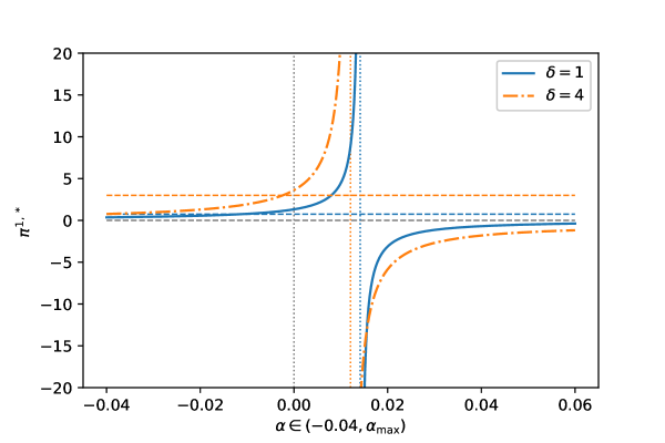
Figure 1. Illustration of $\pi^{1,*}$ from Theorem 3.3 in terms of $\alpha\in(-0.04,\alpha_{\text{max}})$ for $n=12$, $\mu=0.03$, $\sigma=0.2$ and $\alpha_{\text{max}}=n\sigma^{2}/8$. $\theta_{1}=0.3,\,\delta_{1}\in\{1,4\}$ and the parameters $\theta_{j}$ and $\delta_{j}$, $j\geq 2$ are increasing from $0$ to $1$ with step size $0.1$ and from $0.5$ to $2.7$ by step size $0.2$, respectively.

4. Optimization under CARA utility with nonlinear price impact

At the beginning of Section 2, we assumed that the price impact of the $n$ investors in our financial market is given as a linear function in terms of the arithmetic mean of the $n$ investors’ strategies. While the use of the arithmetic mean seems intuitive and reasonable since we assumed that investors are ’small’, one could ask whether using a different function than a linear one would lead to a different optimization problem and hence also a different optimal investment.

In Theorem 3.3 we were able to find an explicit solution to the associated multi-objective portfolio optimization problem using exponential utility (if the parameters are chosen accordingly). The proof highly relies on the linearity of the price impact, so we will not be able to give an explicit solution to the resulting optimization problem in general. However, we will discuss that using a function $g$ that grows superlinearly yields a problem that does not have a finite optimal solution while a function $g$ that grows sublinearly yields a finite optimal solution. If $g$ is a linear function, it depends on the parameter choices whether or not there exists a finite optimal solution (cf. Theorem 3.3). Since, in the linear case, the optimally invested amount is close to zero for decreasing price impact (i.e. if $\alpha<0$, see Theorem 3.3 and Figure 1) we only consider price impact which is increasing in order size.

More explicitly, the price impact will now be modeled by some strictly increasing and continuous function $g:\mathbb{R}\to\mathbb{R}$ with $g(0)=0$. Therefore, the stock price process will be given as the solution to the SDE

$$\mathrm{d}S_{t}=S_{t}\left(\left(\mu+g\left(\bar{\pi}_{t}\right)\right)\mathrm{d}t+\sigma\mathrm{d}W_{t}\right),\,S_{0}=1,$$ (4.1)

which is, of course, still just a stochastic exponential.

As before, we have to restrict ourselves to constant Nash equilibria. Therefore, from the view of investor $i$, we can rewrite the expression $g(\bar{\pi}_{t})$ in the previous SDE as follows

$$g(\bar{\pi}_{t})=g\left(\frac{1}{n}\sum_{j=1}^{n}\pi^{j}_{t}\right)=g\left(\frac{1}{n}\pi^{i}_{t}+\frac{1}{n}\sum_{j\neq i}\pi^{j}\right)\eqqcolon\widetilde{g}(\pi^{i}_{t}),$$ (4.2)

where $\widetilde{g}(p)\coloneqq g\left(\frac{p}{n}+\frac{1}{n}\sum_{j\neq i}\pi^{j}\right),\,p\in\mathbb{R}$. Of course, we assumed that the strategies $\pi^{j}$, $j\neq i$, of the other investors are fixed, constant and deterministic. It also follows that $\widetilde{g}$ is still strictly increasing and satisfies $\widetilde{g}\left(-\sum_{j\neq i}\pi^{j}\right)=0$.

Again, strategies $\pi^{i}$ are restricted to the set $\mathcal{A}$ of admissible strategies. In the following, we will prove that

$$\begin{cases}&\sup_{\pi^{i}\in\mathcal{A}}\mathbb{E}\left[-\exp\left(-\frac{1}{\delta_{i}}\left(X_{T}^{i,\pi^{i}}-\frac{\theta_{i}}{n}\sum_{j\neq i}X_{T}^{j,\pi^{j}}\right)\right)\right],\\ \text{s.t. }&X^{i,\pi^{i}}_{T}=x_{0}^{i}+\displaystyle\int_{0}^{T}\pi^{i}_{t}\left(\left(\mu+g(\bar{\pi}_{t})\right)\mathrm{d}t+\sigma\mathrm{d}W_{t}\right),\end{cases}$$ (4.3)

has an optimal solution if $g$ grows sublinearly and there exists no optimal strategy if $g$ grows superlinearly. Here, $\pi^{j}$, $j\neq i$, are assumed to be constant.

The following theorem summarizes the first assertion of this section, which treats the case that $g$ grows superlinearly.

Proposition 4.1.

If $\lim_{x\to\pm\infty}\frac{g(x)}{x}=\infty$, (4.3) does not have an optimal solution.

Proof.

In order to prove that (4.3) does not have an optimal solution, we will prove that, even if we only consider constant strategies for agent $i$, the optimal value is zero and the associated strategy is infinite. If $\pi^{j}$ is constant for all $j\in\{1,\ldots,n\}$, we obtain

$$X_{T}^{i,\pi^{i}}-\frac{\theta_{i}}{n}\sum_{j\neq i}X_{T}^{j,\pi^{j}}$$

$$= x_{0}^{i}-\frac{\theta_{i}}{n}\sum_{j\neq i}x_{0}^{j}+\Big{(}\pi^{i}-\frac{\theta_{i}}{n}\sum_{j\neq i}\pi^{j}\Big{)}(\mu+g(\bar{\pi}))T+\Big{(}\pi^{i}-\frac{\theta_{i}}{n}\sum_{j\neq i}\pi^{j}\Big{)}\sigma W_{T}$$

$$\eqqcolon y_{0}^{i}+\mu(\pi^{i})T+\sigma(\pi^{i})W_{T}.$$

Hence, for fixed $\pi^{j}$, $j=1,\ldots,n$, the value of the objective function in (4.3) is given by

$$\mathbb{E}\Big{[}-\exp\Big{(}-\frac{1}{\delta_{i}}\Big{(}y_{0}^{i}+\mu(\pi^{i})T+\sigma(\pi^{i})W_{T}\Big{)}\Big{)}\Big{]}$$ (4.4)

$$= -\exp\Big{(}-\frac{1}{\delta_{i}}y_{0}^{i}\Big{)}\cdot\exp\Big{(}-\frac{1}{\delta_{i}}\Big{(}\mu(\pi^{i})-\frac{\sigma(\pi^{i})^{2}}{2\delta_{i}}\Big{)}T\Big{)}.$$ (4.5)

Thus, maximizing the objective function of $\eqref{eq:problem_g}$ with respect to constant strategies $\pi^{i}$ is equivalent to maximizing $\mu(\pi^{i})-\frac{\sigma(\pi^{i})^{2}}{2\delta_{i}}.$ Reinserting the definition of $\mu(\pi^{i})$ and $\sigma(\pi^{i})$ yields

$$\mu(\pi^{i})-\frac{\sigma(\pi^{i})^{2}}{2\delta_{i}}$$

$$= \pi^{i}g(\bar{\pi})-\frac{\sigma^{2}}{2\delta_{i}}(\pi^{i})^{2}+\pi^{i}\Big{(}\mu+\frac{\sigma^{2}\theta_{i}}{n\delta_{i}}\sum_{j\neq i}\pi^{j}\Big{)}-\frac{\theta_{i}}{n}g(\bar{\pi})\sum_{j\neq i}\pi^{j}-\frac{\theta_{i}}{n}\sum_{j\neq i}\pi^{j}\Big{(}\mu+\frac{\sigma^{2}\theta_{i}}{2n\delta_{i}}\sum_{j\neq i}\pi^{j}\Big{)}$$

which converges to $\infty$ if $\pi^{i}$ converges to $\pm\infty$ using the assumption that $g$ grows superlinearly. Therefore,

$$0\geq \sup_{\pi^{i}\in\mathcal{A}}\mathbb{E}\Big{[}-\exp\Big{(}-\frac{1}{\delta_{i}}\Big{(}X_{T}^{i,\pi^{i}}-\frac{\theta_{i}}{n}\sum_{j\neq i}X_{T}^{j,\pi^{j}}\Big{)}\Big{)}\Big{]}$$

$$\geq \sup_{\begin{subarray}{c}\pi^{i}\in\mathcal{A}\\ \pi^{i}\text{ constant}\end{subarray}}\mathbb{E}\Big{[}-\exp\Big{(}-\frac{1}{\delta_{i}}\Big{(}X_{T}^{i,\pi^{i}}-\frac{\theta_{i}}{n}\sum_{j\neq i}X_{T}^{j,\pi^{j}}\Big{)}\Big{)}\Big{]}=0.$$

Hence, the optimal value of (4.3) is zero, which implies that the argument inside the exponential function needs to be infinite. Hence, the problem does not have an optimal solution. ∎

As a result we cannot hope for a Nash equilibrium in this case. Now we can consider the case of sublinear growth of $g$. Hence, we assume that

$$\lim_{x\to\pm\infty}\frac{g(x)}{x}=0.$$

Then we can prove that there exists an optimal policy for (4.3). In order to do so, let $a^{*}$ be a maximum point of

$$a\mapsto\Big{(}a-\frac{\theta_{i}}{n}\sum_{j\neq i}\pi^{j}\Big{)}\Big{(}\mu+\widetilde{g}(a)\Big{)}-\frac{\sigma^{2}}{2\delta_{i}}\Big{(}a-\frac{\theta_{i}}{n}\sum_{j\neq i}\pi^{j}\Big{)}^{2}.$$ (4.6)

Due to our assumption on $g$, a maximum point $a^{*}$ exists and is finite. Then we obtain the following result.

Proposition 4.2.

If $\lim_{x\to\pm\infty}\frac{g(x)}{x}=0$, an optimal strategy for (4.3) is given by $\pi_{t}^{i}\equiv a^{*}$, where $a^{*}$ is the maximum point from (4.6).

Proof.

For the moment we restrict to bounded strategies $(\pi_{t}^{i}),$ i.e. there exists a constant $K>0$ such that $|\pi_{t}^{i}|\leq K$ for all $t\in[0,T].$ For constants $\pi^{j}$, we obtain

$$-\frac{1}{\delta_{i}}\Big{(}X_{T}^{i,\pi^{i}}-\frac{\theta_{i}}{n}\sum_{j\neq i}X_{T}^{j,\pi^{j}}\Big{)}$$

$$= -\frac{1}{\delta_{i}}\Big{(}x_{0}^{i}-\frac{\theta_{i}}{n}\sum_{j\neq i}x_{0}^{j}\Big{)}-\frac{1}{\delta_{i}}\Bigg{(}\int_{0}^{T}\Big{(}\pi^{i}_{t}-\frac{\theta_{i}}{n}\sum_{j\neq i}\pi^{j}\Big{)}(\mu+g(\bar{\pi}_{t}))\mathrm{d}t+\sigma\int_{0}^{T}\Big{(}\pi^{i}_{t}-\frac{\theta_{i}}{n}\sum_{j\neq i}\pi^{j}\Big{)}\mathrm{d}W_{t}\Bigg{)}$$

$$-\frac{\sigma^{2}}{2\delta_{i}^{2}}\int_{0}^{T}\Big{(}\pi^{i}_{t}-\frac{\theta_{i}}{n}\sum_{j\neq i}\pi^{j}\Big{)}^{2}\mathrm{d}t+\frac{\sigma^{2}}{2\delta_{i}^{2}}\int_{0}^{T}\Big{(}\pi^{i}_{t}-\frac{\theta_{i}}{n}\sum_{j\neq i}\pi^{j}\Big{)}^{2}\mathrm{d}t.$$

Now define a new probability measure $\mathbb{Q}$ by

$$\frac{\mathrm{d}\mathbb{Q}}{\mathrm{d}\mathbb{P}}=\exp\Bigg{(}-\frac{\sigma^{2}}{2\delta_{i}^{2}}\int_{0}^{T}\Big{(}\pi^{i}_{t}-\frac{\theta_{i}}{n}\sum_{j\neq i}\pi^{j}\Big{)}^{2}\mathrm{d}t-\frac{\sigma}{\delta_{i}}\int_{0}^{T}\Big{(}\pi^{i}_{t}-\frac{\theta_{i}}{n}\sum_{j\neq i}\pi^{j}\Big{)}\mathrm{d}W_{t}\Bigg{)}.$$

Note that this expression is a density since $\pi_{t}^{i}$ is bounded. Thus, we can write the (negative) target function of (4.3) as

$$\mathbb{E}\left[\exp\left(-\frac{1}{\delta_{i}}\left(X_{T}^{i,\pi^{i}}-\frac{\theta_{i}}{n}\sum_{j\neq i}X_{T}^{j,\pi^{j}}\right)\right)\right]=\exp\Bigg{(}-\frac{1}{\delta_{i}}\Big{(}x_{0}^{i}-\frac{\theta_{i}}{n}\sum_{j\neq i}x_{0}^{j}\Big{)}\Bigg{)}$$

$$\cdot\mathbb{E}_{\mathbb{Q}}\left[\exp\Bigg{(}-\frac{1}{\delta_{i}}\Bigg{(}\int_{0}^{T}\Big{(}\pi^{i}_{t}-\frac{\theta_{i}}{n}\sum_{j\neq i}\pi^{j}\Big{)}(\mu+g(\bar{\pi}_{t}))-\frac{\sigma^{2}}{2\delta_{i}}\Big{(}\pi^{i}_{t}-\frac{\theta_{i}}{n}\sum_{j\neq i}\pi^{j}\Big{)}^{2}\mathrm{d}t\Bigg{)}\Bigg{)}\right].$$

But now in order to minimize the expectation we can do this pointwise under the integral which leads to maximizing (4.6). Since the maximizing point is not at the boundary, the assumption of bounded policies is no restriction. Thus, we have solved the problem.

∎

Whether or not a Nash equilibrium exists in this case depends now on the precise choice of $g.$

Remark 4.3.

The structure of the function (4.6) considered in the proof of Proposition 4.2 implies that there exist at least one and at most two global maxima.

5. Optimization under CRRA utility with linear price impact

In this section, we assume that agents use CRRA utility functions (power or logarithmic) to measure their preferences. Hence, we let

$$U_{i}:(0,\infty)\rightarrow\mathbb{R},\,x\mapsto\begin{cases}\left(1-\frac{1}{\delta_{i}}\right)^{-1}x^{1-\frac{1}{\delta_{i}}},\,&\delta_{i}\neq 1,\\ \ln(x),\,&\delta_{i}=1\end{cases}$$ (5.1)

for some preference parameter $\delta_{i}>0$, $i=1,\ldots,n$. By $\ln(\cdot)$ we denote the natural logarithm.

While using CRRA utility functions, it is mathematically more convenient to optimize the invested fraction of wealth instead of the amount or number of shares. Thus, throughout this subsection, $\pi^{i}_{t}$, $i=1,\ldots,n,$ denotes the fraction of agent $i$’s wealth invested into the risky stock at some time $t\in[0,T]$. The wealth process of agent $i$ is therefore given as the solution to the SDE

$$\mathrm{d}X_{t}^{i,\pi^{i}}=X_{t}^{i,\pi^{i}}\pi^{i}_{t}\left(\left(\mu+\alpha\bar{\pi}_{t}\right)\mathrm{d}t+\sigma\mathrm{d}W_{t}\right),\,X_{0}^{i,\pi^{i}}=x_{0}^{i}.$$ (5.2)

Similar to Section 3 in [29], we include the strategic interaction component into our problem by inserting the product of agent $i$’s and a weighted geometric mean of the other agents’ terminal wealth into the expected utility criterion of the portfolio optimization problem. Therefore, the portfolio optimization problem of agent $i$ is given by

$$\begin{cases}&\sup_{\pi^{i}\in\mathcal{A}}\,\mathbb{E}\Bigg{[}\frac{\delta_{i}}{\delta_{i}-1}\Bigg{(}X_{T}^{i,\pi^{i}}\Big{(}\prod_{j\neq i}X_{T}^{j,\pi^{j}}\Big{)}^{-\frac{\theta_{i}}{n}}\Bigg{)}^{\frac{\delta_{i}-1}{\delta_{i}}}\Bigg{]},\\ \text{s.t. }&\mathrm{d}X_{t}^{i,\pi^{i}}=X_{t}^{i,\pi^{i}}\pi^{i}_{t}\left(\left(\mu+\alpha\bar{\pi}_{t}\right)\mathrm{d}t+\sigma\mathrm{d}W_{t}\right),\,X_{0}^{i,\pi^{i}}=x_{0}^{i}.\end{cases}$$ (5.3)

In order to find an explicit solution for the Nash equilibrium we need to restrict ourselves to constant strategies. Since the reduction to some auxiliary problem containing only one instead of all $n$ agents is not possible in this setting, we need to directly solve the best response problem in order to determine the Nash equilibrium. Then the unique constant Nash equilibrium is given in the following theorem.

Theorem 5.1.

Assume that the following assumptions hold

1. $(n+\theta_{i})\left(n\sigma^{2}-\delta_{i}\alpha\right)-\theta_{i}\delta_{i}\sigma^{2}>0$ for all $i=1,\ldots,n$,

2. $n\sigma^{2}-2\delta_{i}\alpha>0$ for all $i=1,\ldots,n$,

3. $1-\sum_{j=1}^{n}\frac{(n-\theta_{j})\alpha\delta_{j}-n\theta_{j}(\delta_{j}-1)\sigma^{2}}{(n+\theta_{j})(n\sigma^{2}-\alpha\delta_{j})-n\theta_{j}\delta_{j}\sigma^{2}}\neq 0$.

Then the unique (up to modifications) constant Nash equilibrium to (5.3) in terms of invested fractions is given by

$$\pi^{i,*}= \frac{n^{2}\delta_{i}\mu}{(n+\theta_{i})(n\sigma^{2}-\delta_{i}\alpha)-n\theta_{i}\delta_{i}\sigma^{2}}+\frac{(n-\theta_{i})\alpha\delta_{i}-n\theta_{i}(\delta_{i}-1)\sigma^{2}}{(n+\theta_{i})(n\sigma^{2}-\delta_{i}\alpha)-n\theta_{i}\delta_{i}\sigma^{2}}$$ (5.4)

$$\cdot\Bigg{(}1-\sum_{j=1}^{n}\frac{(n-\theta_{j})\alpha\delta_{j}-n\theta_{j}(\delta_{j}-1)\sigma^{2}}{(n+\theta_{j})(n\sigma^{2}-\alpha\delta_{j})-n\theta_{j}\delta_{j}\sigma^{2}}\Bigg{)}^{-1}\sum_{j=1}^{n}\frac{n^{2}\delta_{j}\mu}{(n+\theta_{j})(n\sigma^{2}-\delta_{j}\alpha)-n\theta_{j}\delta_{j}\sigma^{2}}.$$ (5.5)

Proof.

Let $i\in\{1,\ldots,n\}$ be arbitrary but fixed and assume that the other agents use constant strategies $\pi^{j}$, $j\neq i$, which will also be assumed to be arbitrary but fixed. Now define the stochastic process $(Y_{t}^{-i})_{t\in[0,T]}$ by $Y_{t}^{-i}=\prod_{j\neq i}X_{t}^{j,\pi^{j}}$, $t\in[0,T]$.

At first, we determine the dynamics of the process $\Big{(}(Y_{t}^{-i})^{-\frac{\theta_{i}}{n}}\Big{)}_{t\in[0,T]}$. To simplify our calculations, we first consider the logarithm of this process. We obtain

$$\ln\Big{(}(Y_{t}^{-i})^{-\frac{\theta_{i}}{n}}\Big{)}=-\frac{\theta_{i}}{n}\sum_{j\neq i}\ln\Big{(}X_{t}^{j,\pi^{j}}\Big{)}$$ (5.6)

for $t\in[0,T]$. The Itô-Doeblin formula implies

$$\mathrm{d}\ln\Big{(}X_{t}^{j,\pi^{j}}\Big{)} =\pi^{j}((\mu+\alpha\bar{\pi}_{t})\mathrm{d}t+\sigma\mathrm{d}W_{t})-\frac{\sigma^{2}}{2}(\pi^{j})^{2}\mathrm{d}t.$$

Hence, using (5.6),

$$\mathrm{d}\Big{(}\ln\Big{(}(Y_{t}^{-i})^{-\frac{\theta_{i}}{n}}\Big{)}\Big{)}=-\frac{\theta_{i}}{n}\sum_{j\neq i}\pi^{j}((\mu+\alpha\bar{\pi}_{t})\mathrm{d}t+\sigma\mathrm{d}W_{t})+\frac{\theta_{i}}{n}\frac{\sigma^{2}}{2}\sum_{j\neq i}(\pi^{j})^{2}\mathrm{d}t.$$

Using the Itô-Doeblin formula a second time then yields

$$\mathrm{d}\Big{(}(Y_{t}^{-i})^{-\frac{\theta_{i}}{n}}\Big{)}=\mathrm{d}\Big{(}\exp\Big{(}\ln\Big{(}(Y_{t}^{-i})^{-\frac{\theta_{i}}{n}}\Big{)}\Big{)}\Big{)}$$

$$= \,(Y_{t}^{-i})^{-\frac{\theta_{i}}{n}}\left(-\frac{\theta_{i}}{n}\sum_{j\neq i}\pi^{j}((\mu+\alpha\bar{\pi}_{t})\mathrm{d}t+\sigma\mathrm{d}W_{t})+\frac{\sigma^{2}}{2}\frac{\theta_{i}}{n}\sum_{j\neq i}(\pi^{j})^{2}\mathrm{d}t+\frac{\sigma^{2}}{2}\Big{(}\frac{\theta_{i}}{n}\Big{)}^{2}\Big{(}\sum_{j\neq i}\pi^{j}\Big{)}^{2}\mathrm{d}t\right).$$

Hence, we can use partial integration to find the dynamics of the process associated to the argument of the utility function in (5.3):

$$\mathrm{d}\Big{(}X_{t}^{i,\pi^{i}}(Y_{t}^{-i})^{-\frac{\theta_{i}}{n}}\Big{)}$$

$$= X_{t}^{i,\pi^{i}}\left(Y_{t}^{-i}\right)^{-\frac{\theta_{i}}{n}}\Bigg{(}-\frac{\theta_{i}}{n}\sum_{j\neq i}\pi^{j}((\mu+\alpha\bar{\pi}_{t})\mathrm{d}t+\sigma\mathrm{d}W_{t})+\frac{\sigma^{2}}{2}\frac{\theta_{i}}{n}\sum_{j\neq i}(\pi^{j})^{2}\mathrm{d}t+\frac{\sigma^{2}}{2}\Big{(}\frac{\theta_{i}}{n}\Big{)}^{2}\Big{(}\sum_{j\neq i}\pi^{j}\Big{)}^{2}\mathrm{d}t$$

$$+\pi^{i}_{t}((\mu+\alpha\bar{\pi}_{t})\mathrm{d}t+\sigma\mathrm{d}W_{t})-\frac{\theta_{i}}{n}\sigma^{2}\pi^{i}_{t}\sum_{j\neq i}\pi^{j}\mathrm{d}t\Bigg{)}$$

$$= X_{t}^{i,\pi^{i}}\left(Y_{t}^{-i}\right)^{-\frac{\theta_{i}}{n}}\Bigg{(}\pi^{i}_{t}(\mu\mathrm{d}t+\sigma\mathrm{d}W_{t})+\frac{\alpha}{n}(\pi^{i}_{t})^{2}\mathrm{d}t+\Big{(}\frac{\alpha}{n}-\frac{\alpha\theta_{i}}{n^{2}}-\frac{\theta_{i}}{n}\sigma^{2}\Big{)}\pi^{i}_{t}\sum_{j\neq i}\pi^{j}\mathrm{d}t$$

$$+\Big{(}\sum_{j\neq i}\pi^{j}\Big{)}^{2}\frac{\theta_{i}}{n}\Big{(}\frac{\theta_{i}}{2n}\sigma^{2}-\frac{\alpha}{n}\Big{)}\mathrm{d}t-\frac{\theta_{i}}{n}\sum_{j\neq i}\pi^{j}(\mu\mathrm{d}t+\sigma\mathrm{d}W_{t})+\frac{\theta_{i}}{2n}\sigma^{2}\sum_{j\neq i}(\pi^{j})^{2}\mathrm{d}t\Bigg{)},$$

where we used the last step to separate the summands depending on $\pi^{i}$ from the ones that do not depend on $\pi^{i}$. Now a simple caluculation yields that we can rewrite

$$X_{t}^{i,\pi^{i}}\cdot\left(Y_{t}^{-i}\right)^{-\frac{\theta_{i}}{n}}=\widetilde{X}^{i,\pi^{i}}_{t}\cdot\left(\widetilde{Y}^{-i}_{t}\right)^{-\frac{\theta_{i}}{n}},$$ (5.7)

where the process $\widetilde{Y}^{-i}$ does not depend on $\pi^{i}$. More specifically, the dynamics of $\widetilde{X}^{i,\pi^{i}}$ and $\widetilde{Y}^{-i}$ are given by

$$\mathrm{d}\widetilde{X}^{i,\pi^{i}}_{t} =\widetilde{X}^{i,\pi^{i}}_{t}\pi^{i}_{t}\Bigg{(}\Big{(}\mu+\frac{\alpha}{n}\pi^{i}_{t}+\frac{\alpha}{n}\Big{(}1-\frac{\theta_{i}}{n}\Big{)}\sum_{j\neq i}\pi^{j}\Big{)}\mathrm{d}t+\sigma\mathrm{d}W_{t}\Bigg{)},$$

$$\mathrm{d}\widetilde{Y}^{-i}_{t} =\widetilde{Y}^{-i}_{t}\Bigg{(}\sum_{j\neq i}\pi^{j}\Big{(}\Big{(}\mu+\frac{\alpha}{n}\sum_{j\neq i}\pi^{j}\Big{)}\mathrm{d}t+\sigma\mathrm{d}W_{t}\Big{)}+\frac{\sigma^{2}}{2}\Big{(}\sum_{j\neq i}\pi^{j}\Big{)}^{2}\mathrm{d}t-\frac{\sigma^{2}}{2}\sum_{j\neq i}(\pi^{j})^{2}\mathrm{d}t\Bigg{)}$$

with $\widetilde{X}_{0}^{i,\pi^{i}}=x_{0}^{i},\,\widetilde{Y}_{0}^{-i}=\prod_{j\neq i}x_{0}^{j}.$

The previously introduced processes $\widetilde{X}^{i,\pi^{i}}$ and $\widetilde{Y}^{-i}$ simplify the derivation of the HJB-equation in this setting. In order to derive a HJB-equation we define the following value function ($t\in[0,T],\,x,y\in(0,\infty)$)

$$v(t,x,y) \coloneqq\sup_{\pi^{i}\in\mathcal{A}}\mathbb{E}\left[\frac{\delta_{i}}{\delta_{i}-1}\left(\widetilde{X}^{i,\pi^{i}}_{T}\left(\widetilde{Y}^{-i}_{T}\right)^{-\frac{\theta_{i}}{n}}\right)^{\frac{\delta_{i}-1}{\delta_{i}}}\Bigg{|}\widetilde{X}^{i,\pi^{i}}_{t}=x,\,\widetilde{Y}^{-i}_{t}=y\right].$$

We can derive a HJB equation using classical arguments (see e.g. [32], [6], [18]) and obtain

$$0= v_{t}+yv_{y}\Bigg{\{}\sum_{j\neq i}\pi^{j}\Big{(}\mu+\frac{\alpha}{n}\sum_{j\neq i}\pi^{j}\Big{)}+\frac{\sigma^{2}}{2}\Big{(}\sum_{j\neq i}\pi^{j}\Big{)}^{2}-\frac{\sigma^{2}}{2}\sum_{j=1}^{n}(\pi^{j})^{2}\Bigg{\}}+\frac{\sigma^{2}}{2}y^{2}v_{yy}\Big{(}\sum_{j\neq i}\pi^{j}\Big{)}^{2}$$

$$+\sup_{\pi^{i}\in\mathbb{R}}\Bigg{\{}xv_{x}\pi^{i}\mu+\left(\frac{\alpha}{n}\left(1-\frac{\theta_{i}}{n}\right)xv_{x}+\sigma^{2}xyv_{xy}\right)\pi^{i}\sum_{j\neq i}\pi^{j}+\Big{(}\frac{\alpha}{n}xv_{x}+\frac{\sigma^{2}}{2}x^{2}v_{xx}\Big{)}(\pi^{i})^{2}\Bigg{\}},$$

where we omitted the arguments of $v$ and its derivatives for notational convenience. The supremum is attained at

$$\pi^{i,*}=-\frac{xv_{x}\mu+\Big{(}\frac{\alpha}{n}\Big{(}1-\frac{\theta_{i}}{n}\Big{)}xv_{x}+\sigma^{2}xyv_{xy}\Big{)}\sum_{j\neq i}\pi^{j}}{2\Big{(}\frac{\alpha}{n}xv_{x}+\frac{\sigma^{2}}{2}x^{2}v_{xx}\Big{)}},$$ (5.8)

which reduces the HJB equation to the PDE

$$0= v_{t}+yv_{y}\Bigg{\{}\sum_{j\neq i}\pi^{j}\Big{(}\mu+\frac{\alpha}{n}\sum_{j\neq i}\pi^{j}\Big{)}+\frac{\sigma^{2}}{2}\Big{(}\sum_{j\neq i}\pi^{j}\Big{)}^{2}-\frac{\sigma^{2}}{2}\sum_{j=1}^{n}(\pi^{j})^{2}\Bigg{\}}+\frac{\sigma^{2}}{2}y^{2}v_{yy}\Big{(}\sum_{j\neq i}\pi^{j}\Big{)}^{2}$$

$$-\frac{\Big{(}xv_{x}\mu+\Big{(}\frac{\alpha}{n}\Big{(}1-\frac{\theta_{i}}{n}\Big{)}xv_{x}+\sigma^{2}xyv_{xy}\Big{)}\sum_{j\neq i}\pi^{j}\Big{)}^{2}}{4\Big{(}\frac{\alpha}{n}xv_{x}+\frac{\sigma^{2}}{2}x^{2}v_{xx}\Big{)}}$$

with terminal condition

$$v(T,x,y)=\frac{\delta_{i}}{\delta_{i}-1}\Big{(}xy^{-\frac{\theta_{i}}{n}}\Big{)}^{\frac{\delta_{i}-1}{\delta_{i}}},\,x,y>0.$$ (5.9)

For the solution, we make the following ansatz for $v$

$$v(t,x,y)=f(t)\frac{\delta_{i}}{\delta_{i}-1}\Big{(}xy^{-\frac{\theta_{i}}{n}}\Big{)}^{\frac{\delta_{i}-1}{\delta_{i}}}$$ (5.10)

for some continuously differentiable function $f:[0,T]\to(0,\infty)$ with $f(T)=1$. Hence, inserting the ansatz for $v$ reduces the HJB equation to the ODE

$$0=f^{\prime}(t)+\rho f(t)$$ (5.11)

with terminal condition $f(T)=1$, where we defined the constant

$$\rho= -\frac{\theta_{i}}{n}\frac{\delta_{i}-1}{\delta_{i}}\Bigg{(}\sum_{j\neq i}\pi^{j}\Big{(}\mu+\frac{\alpha}{n}\sum_{j\neq i}\pi^{j}\Big{)}+\frac{\sigma^{2}}{2}\Big{(}\sum_{j\neq i}\pi^{j}\Big{)}^{2}-\frac{\sigma^{2}}{2}\sum_{j=1}^{n}(\pi^{j})^{2}\Bigg{)}$$

$$+\frac{\sigma^{2}}{2}\frac{\theta_{i}}{n}\frac{\delta_{i}-1}{\delta_{i}}\Big{(}1+\frac{\theta_{i}}{n}\frac{\delta_{i}-1}{\delta_{i}}\Big{)}\Big{(}\sum_{j\neq i}\pi^{j}\Big{)}^{2}-\frac{\Big{(}n\delta_{i}\mu+\Big{(}\alpha\delta_{i}\Big{(}1-\frac{\theta_{i}}{n}\Big{)}-\sigma^{2}\theta_{i}(\delta_{i}-1)\Big{)}\sum_{j\neq i}\pi^{j}\Big{)}^{2}}{4\Big{(}n\sigma^{2}-2\alpha\delta_{i}\Big{)}^{2}}.$$

The unique solution to (5.11) is given by

$$f(t)=e^{\rho(T-t)},\,t\in[0,T].$$ (5.12)

Inserting the solution $v$ of the HJB equation into the maximizer $\pi^{i,*}$ yields

$$\pi^{i,*}=\frac{n\delta_{i}\mu+\Big{(}\alpha\delta_{i}\Big{(}1-\frac{\theta_{i}}{n}\Big{)}-\sigma^{2}\theta_{i}(\delta_{i}-1)\Big{)}\sum_{j\neq i}\pi^{j}}{n\sigma^{2}-2\alpha\delta_{i}}.$$ (5.13)

Application of a standard verification theorem (see for example [32], [18], [6] for similar arguments) implies that $\pi^{i,*}$ is the unique solution to the best response problem. Moreover, since $\pi^{j}$ were assumed to be constant, $\pi^{i,*}$ is constant, as well. To conclude the proof, we need to solve the system of linear equations defined by (5.13) for $i=1,\ldots,n$. By adding an appropriate multiple of $\pi^{i}$ on both sides and simplifying the equation, we obtain

$$\pi^{i}=\frac{n\delta_{i}\mu}{(n+\theta_{i})\Big{(}\sigma^{2}-\frac{\delta_{i}\alpha}{n}\Big{)}-\sigma^{2}\theta_{i}\delta_{i}}+\frac{\alpha\delta_{i}\Big{(}1-\frac{\theta_{i}}{n}\Big{)}-\sigma^{2}\theta_{i}(\delta_{i}-1)}{(n+\theta_{i})\Big{(}\sigma^{2}-\frac{\delta_{i}\alpha}{n}\Big{)}-\sigma^{2}\theta_{i}\delta_{i}}\sum_{j=1}^{n}\pi^{j}.$$ (5.14)

Summing over all $i\in\{1,\ldots,n\}$ on both sides and solving for $\sum_{j=1}^{n}\pi^{j}$ then yields

$$\sum_{j=1}^{n}\pi^{j}=\Bigg{(}1-\sum_{j=1}^{n}\frac{\alpha\delta_{j}\Big{(}1-\frac{\theta_{j}}{n}\Big{)}-\sigma^{2}\theta_{j}(\delta_{j}-1)}{(n+\theta_{j})\Big{(}\sigma^{2}-\frac{\delta_{j}\alpha}{n}\Big{)}-\sigma^{2}\theta_{j}\delta_{j}}\Bigg{)}^{-1}\sum_{j=1}^{n}\frac{n\delta_{j}\mu}{(n+\theta_{j})\Big{(}\sigma^{2}-\frac{\delta_{j}\alpha}{n}\Big{)}-\sigma^{2}\theta_{j}\delta_{j}}$$ (5.15)

Finally, inserting (5.15) into (5.14) yields the unique constant Nash equilibrium given by ($i=1,\ldots,n$)

$$\pi^{i,*}= \frac{n\delta_{i}\mu}{(n+\theta_{i})\Big{(}\sigma^{2}-\frac{\delta_{i}\alpha}{n}\Big{)}-\sigma^{2}\theta_{i}\delta_{i}}+\frac{\alpha\delta_{i}\Big{(}1-\frac{\theta_{i}}{n}\Big{)}-\sigma^{2}\theta_{i}(\delta_{i}-1)}{(n+\theta_{i})\Big{(}\sigma^{2}-\frac{\delta_{i}\alpha}{n}\Big{)}-\sigma^{2}\theta_{i}\delta_{i}}$$

$$\cdot\Bigg{(}1-\sum_{j=1}^{n}\frac{\alpha\delta_{j}\Big{(}1-\frac{\theta_{j}}{n}\Big{)}-\sigma^{2}\theta_{j}(\delta_{j}-1)}{(n+\theta_{j})\Big{(}\sigma^{2}-\frac{\delta_{j}\alpha}{n}\Big{)}-\sigma^{2}\theta_{j}\delta_{j}}\Bigg{)}^{-1}\sum_{j=1}^{n}\frac{n\delta_{j}\mu}{(n+\theta_{j})\Big{(}\sigma^{2}-\frac{\delta_{j}\alpha}{n}\Big{)}-\sigma^{2}\theta_{j}\delta_{j}}.$$

∎

Remark 5.2.

Similar to Remark 3.4, Theorem 5.1 contains the special cases $\alpha=0$ and $\theta_{i}=0$, $i=1,\ldots,n$. For $\alpha=0$ (no price impact), we deduce

$$\pi^{i,*}=\Bigg{(}\frac{n\delta_{i}}{n+\theta_{i}(1-\delta_{i})}+\frac{\theta_{i}(1-\delta_{i})}{n+\theta_{i}(1-\delta_{i})}\cdot\frac{\sum_{j=1}^{n}\frac{n\delta_{j}}{n+\theta_{j}(1-\delta_{j})}}{1-\sum_{j=1}^{n}\frac{\theta_{j}(1-\delta_{j})}{n+\theta_{j}(1-\delta_{j})}}\Bigg{)}\cdot\frac{\mu}{\sigma^{2}},$$ (5.16)

$i=1,\ldots,n$. In the special case without relative concerns inside the objective function, we obtain

$$\pi^{i,*}=\frac{n\delta_{i}\mu}{n\sigma^{2}-\delta_{i}\alpha}+\frac{\alpha\delta_{i}}{n\sigma^{2}-\delta_{i}\alpha}\cdot\frac{\sum_{j=1}^{n}\frac{n\delta_{j}\mu}{n\sigma^{2}-\alpha\delta_{j}}}{1-\sum_{j=1}^{n}\frac{\alpha\delta_{j}}{n\sigma^{2}-\alpha\delta_{j}}},$$ (5.17)

$i=1,\ldots,n.$ A comparison with Remark 3.4 shows that the Nash equilibria in the special case of $\theta_{i}=0$ for all $i=1,\ldots,n$ are actually the same, although $\pi^{i,*}$ represents the invested amount for exponential and the invested fraction for power utility.

6. Conclusion

In this paper we derive Nash equilibria for agents with relative performance measures in financial markets with price impact. We show that as long as the price impact is not more than linear, the individual optimization problems are well-defined. Whereas without price impact, the agents would always invest a positive amount in the stock in our model, the situation changes dramatically when the price impact is beyond a certain threshold. Then the agents massively short-sell the stock and try to take advantage of falling prices. Thus, a larger price impact leads to a more aggressive behavior of the agents in our model.

Acknoledgement: The authors would like to thank Dirk Becherer and Johannes Muhle-Karbe for helpful discussions and hints to literature.

Statements and Declarations: The authors have no relevant financial or non-financial interests to disclose.

References

- [1] Robert Almgren and Neil Chriss, Optimal execution of portfolio transactions, Journal of Risk 3 (2001), 5–40.
- [2] Peter Bank and Dietmar Baum, Hedging and portfolio optimization in financial markets with a large trader, Mathematical Finance: An International Journal of Mathematics, Statistics and Financial Economics 14 (2004), no. 1, 1–18.
- [3] Suleyman Basak and Dmitry Makarov, Competition among portfolio managers and asset specialization, Paris December 2014, Finance Meeting EUROFIDAI-AFFI Paper (2015).
- [4] Nicole Bäuerle and Tamara Göll, Nash equilibria for relative investors via no-arbitrage arguments, Mathematical Methods of Operations Research (2022), 1–23.
- [5] Dimitris Bertsimas and Andrew W Lo, Optimal control of execution costs, Journal of Financial Markets 1 (1998), no. 1, 1–50.
- [6] Tomas Björk, Arbitrage theory in continuous time, 2. ed., Oxford University Press, 2004.
- [7] Jean-Philippe Bouchaud, Price impact, arXiv:0903.2428 (2009).
- [8] Stephen J. Brown, William N. Goetzmann, and James Park, Careers and survival: Competition and risk in the hedge fund and CTA industry, The Journal of Finance 56 (2001), no. 5, 1869–1886.
- [9] Henrik Cronqvist and Rüdiger Fahlenbrach, Large shareholders and corporate policies, The Review of Financial Studies 22 (2008), no. 10, 3941–3976.
- [10] Domenico Cuoco and Jakša Cvitanić, Optimal consumption choices for a ‘large’investor, Journal of Economic Dynamics and Control 22 (1998), no. 3, 401–436.
- [11] Giuliano Curatola, Portfolio choice of large investors who interact strategically, Available at SSRN 3404491 (2019).
- [12] by same author, Price impact, strategic interaction and portfolio choice, The North American Journal of Economics and Finance 59 (2022), 101594.
- [13] Jakša Cvitanić and Jin Ma, Hedging options for a large investor and forward-backward sde’s, The Annals of Applied Probability 6 (1996), no. 2, 370–398.
- [14] Goncalo Dos Reis and Vadim Platonov, Forward utilities and mean-field games under relative performance concerns, From Particle Systems to Partial Differential Equations, Springer, 2019, pp. 227–251.
- [15] by same author, Forward utility and market adjustments in relative investment-consumption games of many players, arXiv:2012.01235 (2020).
- [16] Zehra Eksi and Hyejin Ku, Portfolio optimization for a large investor under partial information and price impact, Mathematical Methods of Operations Research 86 (2017), 601–623.
- [17] Gilles-Edouard Espinosa and Nizar Touzi, Optimal investment under relative performance concerns, Mathematical Finance 25 (2015), no. 2, 221–257.
- [18] Wendell H Fleming and Halil Mete Soner, Controlled markov processes and viscosity solutions, vol. 25, Springer Science & Business Media, 2006.
- [19] Guanxing Fu, Xizhi Su, and Chao Zhou, Mean field exponential utility game: A probabilistic approach, arXiv:2006.07684 (2020).
- [20] Hua He and Harry Mamaysky, Dynamic trading policies with price impact, Journal of Economic Dynamics and Control 29 (2005), no. 5, 891–930.
- [21] Ruimeng Hu and Thaleia Zariphopoulou, -player and mean-field games in It-diffusion markets with competitive or homophilous interaction, arXiv:2106.00581 (2021).
- [22] Robert A Jarrow, Market manipulation, bubbles, corners, and short squeezes, Journal of Financial and Quantitative Analysis 27 (1992), no. 3, 311–336.
- [23] by same author, Derivative security markets, market manipulation, and option pricing theory, Journal of Financial and Quantitative Analysis 29 (1994), no. 2, 241–261.
- [24] Ioannis Karatzas and Steven E. Shreve, Methods of mathematical finance, vol. 39, Springer, 1998.
- [25] Alexander Kempf and Stefan Ruenzi, Tournaments in mutual-fund families, The Review of Financial Studies 21 (2008), no. 2, 1013–1036.
- [26] Holger Kraft and Christoph Kühn, Large traders and illiquid options: Hedging vs. manipulation, Journal of Economic Dynamics and Control 35 (2011), no. 11, 1898–1915.
- [27] Holger Kraft, André Meyer-Wehmann, and Frank Thomas Seifried, Dynamic asset allocation with relative wealth concerns in incomplete markets, Journal of Economic Dynamics and Control 113 (2020), 103857.
- [28] Daniel Lacker and Agathe Soret, Many-player games of optimal consumption and investment under relative performance criteria, Mathematics and Financial Economics 14 (2020), no. 2, 263–281.
- [29] Daniel Lacker and Thaleia Zariphopoulou, Mean field and -agent games for optimal investment under relative performance criteria, Mathematical Finance 29 (2019), no. 4, 1003–1038.
- [30] Hong Liu and Jiongmin Yong, Option pricing with an illiquid underlying asset market, Journal of Economic Dynamics and Control 29 (2005), no. 12, 2125–2156.
- [31] Johannes Muhle-Karbe, Zexin Wang, and Kevin Webster, Stochastic liquidity as a proxy for nonlinear price impact, Available at SSRN 4286108 (2022).
- [32] Huyên Pham, Continuous-time stochastic control and optimization with financial applications, vol. 61, Springer Science & Business Media, 2009.
- [33] Torsten Schöneborn and Alexander Schied, Liquidation in the face of adversity: stealth vs. sunshine trading, EFA 2008 Athens Meetings Paper, 2009.