Microscopic calculation of the pinning energy of a vortex in the inner crust of a neutron star

Abstract

The structure of a vortex in the inner crust of a pulsar is calculated microscopically in the Wigner-Seitz cell approximation, simulating the conditions of the inner crust of a cold, non-accreting neutron star, in which a lattice of nuclei coexists with a sea of superfluid neutrons. The calculation is based on the axially deformed Hartree-Fock-Bogolyubov framework, using effective interactions. The present work extends and improves previous studies in four ways: i) it allows for the axial deformation of protons induced by the large deformation of neutrons due to the appearance of vortices; ii) it includes the effect of Coulomb exchange; iii) considers the possible effects of the screening of the pairing interaction; and iv) it improves the numerical treatment. We also demonstrate that the binding energy of the nucleus-vortex system can be used as a proxy to the pinning energy of a vortex and discuss in which conditions this applies. From our results, we can estimate the mesoscopic pinning forces per unit length acting on vortices. We obtain values ranging between $10^{14}$ to $10^{16}$ dyn/cm, consistent with previous findings.

I Introduction

Pulsars are characterized by the regular emission of electromagnetic radiation. These stars spin down steadily, but sudden spin-ups, called glitches, have been observed. Such events were recorded first in the Vela pulsar and subsequently in many other stars (see Fuentes, J. R. et al. (2017) for a statistical study of the properties of glitches observed in 141 stars). Soon after the first observations, it was proposed that the glitch phenomenon was closely associated with the existence of a neutron superfluid in the interior of the star Baym et al. (1969), see Haskell and Melatos (2015); Antonelli et al. (2022) for a review. According to the current theoretical understanding of neutron star structure, the layer extending from a density of about $10^{-3}$ fm^-3 to 0.04 fm^-3, called the inner crust, is composed of a lattice of heavy nuclei immersed in a sea of free neutrons and electrons Chamel and Haensel (2008); Haensel et al. (2007). Negele and Vautherin carried out a seminal study Negele and Vautherin (1973) within the Wigner-Seitz approximation. They determined the optimal radius of a spherical cell with a nucleus at its center, the number of protons and of neutrons bound to the nucleus and the number of unbound neutrons, as a function of the neutron density at the edges of the cell. Their results have been refined and extended in many subsequent works, see Pizzochero et al. (2002); Sandulescu et al. (2004); Baldo et al. (2007); Grill et al. (2011); Pastore et al. (2011); Mondal et al. (2020); Shelley and Pastore (2021) and references therein. Moreover, given the typical range of temperature expected in the inner crust of mature neutron stars (from $10^{7}$ to $10^{9}$ K, that is from 1 to 100 keV, a very low value with respect to the Fermi energy ranging from 10 to 100 MeV), neutrons are likely to be superfluid Sedrakian and Clark (2019).

Due to the rotation of the star, the superfluid neutrons form a (possibly disordered) array of quantum vortices Feynman (1998), whose average density is closely linked to the pulsar angular velocity via a generalization of the so-called Feynman-Onsager relation Antonelli et al. (2018). Anderson and Itoh Anderson and Itoh (1975) proposed that the interaction between the heavy nuclei at the lattice sites and the vortices can anchor the vortices in particularly energetically favourable positions, a phenomenon referred to as “pinning”. If this is the case, the superfluid component cannot follow the regular slowdown of the crust and rotates faster, becoming a reservoir of angular momentum. This gives rise to hydrodynamical lift forces (Magnus forces), which act on the vortex lines and tend to push them away from their sites. The glitch phenomenon would then occur when Magnus forces take over and a catastrophically large number of vortices suddenly unpin from their positions, releasing their angular momentum to the crust.

There are still some unanswered questions regarding several central aspects of this model. First of all, the trigger which leads to the collective vortex unpinning is not well established yet; there are several possibilities advanced in the literature, like vortex avalanches Anderson and Itoh (1975); Warszawski and Melatos (2013) or hydrodynamical instabilities Glampedakis and Andersson (2009); Khomenko et al. (2019). Secondly, it has been pointed out that the angular momentum contained in the crust may not be sufficient Andersson et al. (2012); Chamel (2013) to explain glitches, albeit this conclusion is less clear if the statistical uncertainty on the observed glitch activity Montoli et al. (2021) or the possible presence of lattice defects Sauls et al. (2020) are taken into account. Finally, there is no definitive answer on the strength of the pinning interaction throughout the inner crust. The greater the ability of pinning to withstand the hydrodynamical lift, the higher the amount of angular momentum that the superfluid can store, so that it is possible to constrain the unpinning threshold (i.e. the theoretical upper limit of the distribution of pinning forces Antonelli and Haskell (2020)) with observations of large glitches Antonelli et al. (2018).

The microscopic computation of the single-nucleus pinning potential is very challenging and has never been performed in the literature. In fact, existing studies resorted to the pinning energy Donati and Pizzochero (2006); Avogadro et al. (2008); Epstein and Baym (1988), defined as the energy difference between two extreme situations: one where the vortex is on top of the nucleus (nuclear pinning), and one where the vortex is equidistant between two adjacent nuclei in the lattice (interstitial pinning). A negative (positive) value of this quantity indicates that the former (latter) situation is energetically favourable.

Different methods have been used to estimate the single-nucleus pinning potential. Epstein and Baym  Epstein and Baym (1988) used hydrodynamic considerations in combination with the Ginzburg–Landau theory of superfluidity to compute the free energy of a nucleus as a function of the distance from a vortex line, ignoring the internal structure of the nucleus and using instead schematic expressions for the kinetic and condensation energies. They found that vortices pin on nuclei in the deeper layers of the inner crust, while they are repelled in the low-density regions. The model by Epstein and Baym was later improved Donati and Pizzochero (2004), providing estimates of pinning energies obtained by making use of a semiclassical treatment based on the Local Density Approximation Donati and Pizzochero (2006).

The first microscopical quantum calculation was then carried out by Avogadro et al. (2008, 2007), based on the solution of the axially symmetric Hartree-Fock-Bogoliubov (HFB) equations in the Wigner-Seitz approximation for various densities in the crust. Specifically, it was found that the nuclear shell structure has relevant effects on the spatial configuration of the vortex and that pinning occurs only in the less dense regions of the inner crust. The solution of the HFB equations was carried out assuming spherical symmetry for the proton density, thus breaking self-consistency. In the present paper, we remove this assumption, which was based on the fact that proton orbitals are deeply bound. Furthermore, we include the effect of the Coulomb exchange, which was previously neglected, and improve the numerical treatment, devoting particular attention to the convergence of our results. We are then able to present new and more reliable values of the binding energy and, based on them, we present our best estimation of the pinning energy. We also show detailed results for neutron and proton deformation at different densities. We also study the dependence of our results on the strength of the pairing interaction, in keeping with the analysis carried out in Donati and Pizzochero (2006).

Due to the fact that hydrodynamics is non-linear, the pinning potential is not immediately related to the pinning “landscape” that defines the dynamics of a finite-size vortex segment Antonelli and Haskell (2020). We then estimate the typical strength of the pinning landscape by taking the mean value of the pinning force for unit length acting on a vortex line Seveso et al. (2016), see also the discussion in Antonelli and Haskell (2020).

Other recent efforts, based on a microscopic quantal picture, have also been made. The most significant advance concerns a three-dimensional dynamical simulation of the vortex motion, based on the time-dependent superfluid local density approximation (TDSLDA), leading to an estimate of the force between the vortex and the nucleus as a function of their separation Wlazłowski et al. (2016); Bulgac et al. (2013)(see also Link (2009)). Results were obtained for two densities and showed that the vortex is repelled by nuclei. At the same time, it was found that the vortex-nucleus interactions induce a deformation of the nucleus and lead to a bending of the vortex line shape. These findings represent an important confirmation of our results and extend them toward a complete characterization of the vortex-nucleus interaction. On the other hand, TDSLDA computations are very costly, while we are able to present systematic calculations of the pinning energy with different functionals and pairing forces and to provide a detailed description of the nuclear deformation. We also report that the properties of a quantum vortex were recently studied at finite temperature in infinite matter using Brussels-Montreal energy functionals Pecak et al. (2021).

We begin in Section II by explaining the general features of the calculation and giving some details about the computation of the pinning energy. Our results are presented in Section III. Finally, in Section IV we give our closing remarks.

II Method

II.1 General description

In this paper, we expand and improve the work done in Avogadro et al. (2008) (hereafter referred to as Paper I). There, the authors approached the problem of pinning energy by solving the Hartree-Fock-Bogolyubov (HFB) equations in a cylindrical Wigner-Seitz cell of radius $R_{WS}$ and height $h_{WS}$ in four different configurations. HFB equations (also called Bogliubov-De Gennes equations) are well suited to study the pairing properties of quantal inhomogeneous systems, like the inner crust of a neutron star, where a lattice of heavy nuclei coexists with a sea of superfluid neutrons. With this technique both the nuclear potential and the pairing correlations are treated simultaneously and self consistently. Explicitly, the HFB equations read

$$\begin{cases}\left(h(\mathbf{x})-\lambda\right)u_{i}(\mathbf{x})+\Delta(\mathbf{x})v_{i}(\mathbf{x})=E_{i}u_{i}(\mathbf{x})\\ \Delta^{*}(\mathbf{x})u_{i}(\mathbf{x})-\left(h(\mathbf{x})-\lambda\right)v_{i}(\mathbf{x})=E_{i}v_{i}(\mathbf{x})\end{cases}$$ (1)

where $E_{i}$ is the quasi-particle energy of level $i$ and $u_{i}$ and $v_{i}$ are the quasi-particle amplitudes relative to that level, $\lambda$ is the chemical potential, $\Delta(\mathbf{x})$ is the pairing field and $h(\mathbf{x})=T+U^{HF}$ is the single particle Hartree-Fock Hamiltonian, sum of the kinetic term $T$ and the self-consistent potential $U^{HF}$.

From the solutions of (1), one can compute the normal and abnormal densities of the system

$$\begin{split}n(\mathbf{x})=\displaystyle\sum_{i}|v_{i}(\mathbf{x})|^{2}\\ \kappa(\mathbf{x})=\displaystyle\sum_{i}u_{i}(\mathbf{x})v_{i}(\mathbf{x})^{*}\end{split}$$ (2)

from which one can find new $h(\mathbf{x})$ and $\Delta(\mathbf{x})$ which in turn give rise to a new set of equations (1) (see Appendix A). The HFB equations are therefore solved via an iterative process.

As for the interaction chosen in the HF sector, we adopt the Skyrme SLy4 and the SkM* parameterizations (see Chabanat et al. (1997)) and neglect the spin-orbit term, because we expect that the pinning energy is not significantly affected by this term (cf. Paper I and our discussion below).

For the pairing field, we start from a neutron pairing potential, adopting a density-dependent, contact interaction of the form

$$V_{pair}(\mathbf{x},\mathbf{x}^{\prime})=V_{0}\left(1-\eta\left(\frac{n(\mathbf{x})}{0.08}\right)^{a}\right)\delta(\mathbf{x}-\mathbf{x}^{\prime})$$ (3)

where $V_{0}=-481$ MeV$\,\cdot\,$fm³, $\eta=0.7$ and $a=0.45$ have been used. This leads in turn to the pairing field

$$\Delta(\mathbf{x})=-V_{pair}(\mathbf{x},\mathbf{x}^{\prime})\kappa(\mathbf{x})$$ (4)

The adopted parameters, together with a cutoff energy $E_{cut}=$ 60 MeV, reproduce the pairing gap of uniform neutron matter as predicted by a realistic nucleon–nucleon interaction Garrido et al. (1999), and are the same as those used in Paper I. We will also perform calculations with two weaker pairing interactions. We aimed for pairing gaps reduced by a factor $\beta=2$ and $\beta=3$; we found $V_{0}^{\beta=2}=432.9$ MeV$\,\cdot\,$fm³ and $V_{0}^{\beta=3}=408.85$ MeV$\,\cdot\,$fm³. These interactions are introduced only to have a rough qualitative assessment of the effects of correlations beyond the mean field, which generally lead to a reduction of the pairing gaps (see Ramanan and Urban (2021); Gandolfi et al. (2022) for recent reviews). However, such reductions show a dependence on the neutron density which is not taken into account by the constant reduction factors considered here. Nonetheless, we will still label the results by $\beta=2$ and $\beta=3$.

The pairing interaction has been neglected in the case of protons since $Z$=40 is used throughout this work and this value corresponds to a magic number in our calculations.

We carry out our calculations in a cylindrical box, so it is natural to use cylindrical coordinates $\mathbf{x}=(\rho,z,\varphi)$. Eqs. (1) are expanded on a single-particle basis. All the calculation details are presented in Appendix A. The pairing field (4) is defined as (Paper I and Gygi and Schlüter (1991))

$$\Delta(\rho,z,\varphi)=\Delta(\rho,z)\,e^{i\nu\varphi}$$ (5)

so that the vortex is created along the $z$-axis keeping the cylindrical symmetry. The integer parameter $\nu$ can be interpreted as the number of units of angular momentum carried by each Cooper pair along the $z-$axis. The standard solution of the HFB equations corresponds to $\nu=0$ and to Cooper pairs coupled to zero angular momentum while $\nu=1$ defines an excited solution in which Cooper pairs of different parity couple to one unit of angular momentum. This solution describes a vortex, as it gives rise to an azimuthal velocity field $V$ of the form

$$V(\rho,z,\varphi)=-\frac{i\hbar}{mn\rho}\displaystyle\sum_{i}v_{i}^{*}(\rho,z,\varphi)\frac{\partial v_{i}(\rho,z,\varphi)}{\partial\varphi}.$$ (6)

It is noted that nuclear shell effects act quite differently on the $\nu=1$ gap, as compared to $\nu=0$. This point is discussed at length in Paper I. In particular, one expects that the spin-orbit interaction, which is neglected in the present work, tends to shift the energy of the single-particle pairs involved in the formation of $S=0,\nu=1$ Cooper pairs by the same amount (see Fig. 21 in Paper I).

We have changed considerably the part of the computation relative to protons with respect to Paper I. In Paper I, the proton density was forced to be spherically symmetric. This was achieved by taking spherical averages of the cylindrical neutron densities to compute the proton potential $U^{HF}_{prot}$ at each step of the iterative process. The reasoning behind this choice was that protons are deeply bound and one does not expect them to be much affected by the neutron density deviation from sphericity. As we will show, this is an accurate approximation only for the outermost layers of the inner crust.

Summarizing, we have extended and improved the calculations of Paper I as follows:

• we add the Coulomb exchange term in the proton potential using the Slater approximation.

• we adopt cylindrical symmetry also in the case of protons.

• we consider, although schematically, the effects associated with the possible reduction of the pairing interaction due to screening effects.

• we improve the numerical aspects of the code, namely the derivation and integration techniques. Improving the numerical precision is crucial for computing the pinning energy, as we will show in the next section.

II.2 Binding and pinning energy

We solve the HFB equations in the following configurations (see Fig. 1 for a sketch):

• Neutron sea (NS): the neutron sea, with neither a nucleus ($Z=0$) nor a vortex ($\nu=0$);

• Nucleus (Nu): a nucleus ($Z\neq 0$) with no vortex ($\nu=0$), surrounded by the neutron sea;

• Interstitial pinning (IP): a vortex ($\nu=1$) with no nucleus ($Z=0$), surrounded by the neutron sea;

• Nuclear pinning (NP): a nucleus ($Z\neq 0$) and a vortex ($\nu=1$) on top of it, surrounded by the neutron sea.

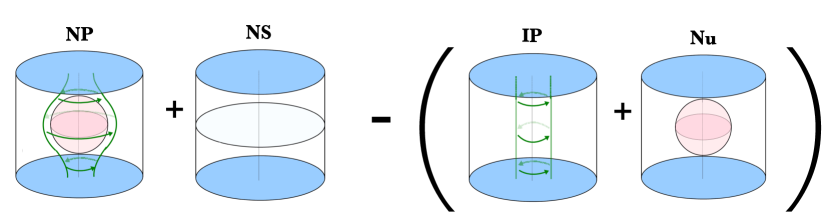
Figure 1: Visual representation of (7). The binding energy is shown as the energy cost to move a vortex from its position on top of a nucleus to an infinite distance from it.

By comparing the total energies of each configuration, we computed the binding energy of the vortex onto the nucleus. This quantity is defined as the difference between the energy needed to build a vortex on top of a nucleus and the energy necessary to build a vortex in uniform matter. Equivalently, the binding energy can be defined as the energy needed to move the vortex from its site on top of the nucleus to an infinite distance from it (see Fig. 1). A negative value means that the favorable position for the vortex is on top of the nucleus, whilst a positive value means that the favorable position is far away from it.

A simple combination of the total energies of each configuration gives the explicit expression of the binding energy

$$E_{b} = E^{NP}+E^{NS}-(E^{IP}+E^{Nu})$$ (7)

$$- \lambda_{n}\left[(N^{NP}+N^{NS}-(N^{IP}+N^{Nu})\right]$$

where $E^{i}$ is the total energy of the specified configuration. We added a correction term proportional to the neutron chemical potential $\lambda_{n}$ to ensure that we compare calculations with the same number of particles, since the vortex, if present, reduces the number of neutrons $N^{i}$ found in each cell.

Numerical precision is crucial to compute the binding energy. The energy terms in (7) range from some hundreds of MeVs up to tens of thousands MeVs as a function of neutron density in the inner crust. The values of the nucleus-vortex binding energy, on the other hand, range from some hundreds of keVs up to tens of MeVs. Even small numerical errors can have substantial effects on the final values of the binding energy.

The binding energy is a different quantity with respect to the pinning energy $E_{p}$. The latter is influenced by the presence of the surrounding nuclear lattice and therefore we are unable to calculate it directly. Nonetheless, we can find an estimate through the binding energy.

Epstein and Baym in Epstein and Baym (1988) realized that there is a kinetic component to the vortex-nucleus interaction, that accounts for the amount of superfluid flow displaced by the nucleus. It reads

$$K_{n}(\rho)=\frac{3}{2}M_{s}\left(\frac{\zeta-1}{\zeta+2}\right)\left(\frac{\hbar}{2m_{0}\rho}\right)^{2}$$ (8)

where $m_{0}$ is the nucleon mass, $M_{s}$ is the mass of the neutron superfluid of density $n_{\infty}$ displaced by a sphere of radius $R_{n}$ (i.e., the nuclear radius) and $\zeta$ is the ratio of the nucleus density $n_{n}$ to the neutron superfluid density $n_{\infty}$. $K_{n}$ is always positive and it is inversely proportional to the square of the distance $\rho$ between the nucleus center and the vortex axis.

On the other hand, the other component of the interaction is of nuclear nature. If we assume that such nuclear interaction is short-ranged, then after a certain critical distance $\rho^{*}$ it will become negligible, along with its contribution to the pinning energy. We can estimate such distance as the sum of the nuclear radius $R_{n}$ and the coherence length $\xi$ of the vortex

$$\rho^{*}\sim R_{n}+\xi$$ (9)

where $\xi=\hbar^{2}k_{F}/\pi m_{0}\Delta$, with $k_{F}$ the Fermi momentum. From our calculations, $\xi$ ranges between 3 and 10 fm approximately, depending on the density of the neutron sea.

To compute the pinning energy, we must compare $\rho^{*}$ with $R_{WS}$. We assume that the nuclear contribution to the vortex-nucleus interaction is negligible for $\rho\gtrsim\rho^{*}$. If $\rho^{*}<R_{WS}$, we then suppose that at $\rho=R_{WS}$ the vortex-nucleus interaction is dominated by the kinetic term (8). Therefore, from the definition of pinning energy, we write

$$E_{p}\simeq E_{b}-K_{n}(R_{WS})$$ (10)

At $R_{WS}$, the contribution of $K_{n}(R_{WS})$ is of the order of a few tens of keV, so that it usually represents a small correction to the pinning energy.

If, on the contrary, $\rho^{*}\gtrsim R_{WS}$, there would still be a substantial overlap between the vortex and the nucleus at a distance $\rho=R_{WS}$. In this case, we are unable to estimate the non-negligible nuclear component to the interaction and therefore we cannot provide an estimate on the pinning energy.

II.3 Computational details

Similarly to Paper I, we present the calculated value of the pinning energy as a function of the density of the neutron sea far from the nucleus, $n_{\infty}$. We investigated eight different density zones, from $n_{\infty}=0.001$ fm^-3 to $n_{\infty}=0.038$ fm^-3. At each density, we have carried out six sets of calculations, using two different Skyrme models, namely SLy4 and SkM*, and three different pairing strengths (marked by the pairing-interaction reduction factor $\beta$). For each set, we iteratively solved two HFB equations, one for protons and one for neutrons, for each of the four different configurations.

The neutron chemical potential was chosen so as to reproduce the external densities predicted in Negele and Vautherin (1973) and studied in Paper I. On the other hand, the proton chemical potential was adjusted to give the proton number $Z=40$ Negele and Vautherin (1973).

We took special care in estimating the errors due to the convergence of the calculations and also those due to the size of the box, which is essential for our results to be reliable. Specifically, we adopted the following convergence criterion for the computation of a given configuration: the program halts when the relative total energy difference between the last and second-last iteration is less than $5\times 10^{-6}$ for three consecutive iteration cycles. In some cases, we observed that this criterion was not stringent enough; we let therefore the computation continue until the relative energy difference reached $5\times 10^{-8}$ for three consecutive iteration cycles.

After the binding energy was obtained, we computed the critical distance $\rho^{*}$ (9) as well as the kinetic contribution (8) (which within our approximation does not depend on the box radius). If the criterion $\rho^{*}<R_{WS}$ was met, we were able to compute the corresponding pinning energies via (10); otherwise, we concluded that our method could not produce a result for the particular parameter set. In Appendix C we show the values of $\rho^{*}$ we obtained.

III Results

III.1 Vortex effects on pairing gaps and proton deformation

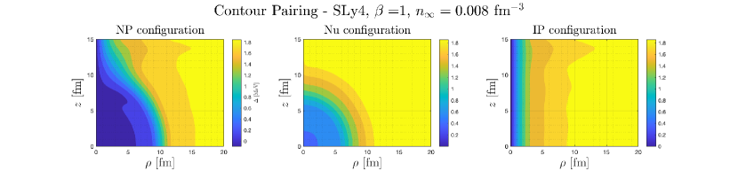
Figure 2: Contour plots of the pairing gaps of the NP (left), Nu (center), and IP (right) configurations.

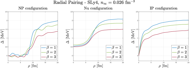
Figure 3: Typical pairing gaps obtained in our calculations for the NP, Nu, and IP configurations, for the SLy4 interactions, and for the three adopted values of $\beta$, as a function of the distance from the vortex axis in the $z=0$ plane.

In Fig. 2 we compare contour plots of the pairing gaps associated with the NP (left), Nu (center), and IP (right) configurations in the $(\rho,z)$ plane, calculated with the SLy4 interaction for the density $n_{\infty}=0.008$ fm^-3. One can see that the gap acquires its asymptotic value for $\rho\gtrsim$ 10 fm in the IP configuration, while the presence of the nucleus distorts the gap profile in the NP configuration so that the vortex enlarges and incorporates the nucleus, and the gap reaches its asymptotic value only for $\rho\gtrsim$ 15 fm. Our results are qualitatively consistent with those obtained in Wlazłowski et al. (2016), where the vortex-nucleus interaction was studied with dynamical simulations (see Fig. 2 in Wlazłowski et al. (2016), where one can actually observe the vortex bending to avoid the nuclear region). The gap profiles for the NP, Nu, and IP configuration along the equator $z=0$ are shown in Fig. 3 for the SLy4 interaction and the three values of $\beta$ we have considered. The density is $n_{\infty}=0.026$ fm^-3. In all cases, the gap is suppressed for $\rho\leq$ 10 fm and rapidly reaches the asymptotic value corresponding to the given value of $\beta$. There is a slight dependence on the interaction, which essentially depends on the different values of the effective mass associated with the SLy4 and with the SkM^∗ interaction.

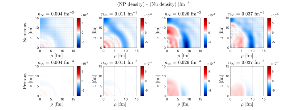
Figure 4: Difference between the densities calculated in the NP and Nu configurations, expressed in fm^-3, as a function of ($\rho,z$) in a $\varphi$-constant plane for several neutron sea densities $n_{\infty}$. In the top half, we show neutron quantities, while in the bottom half proton quantities.

In Fig. 4 we present contour plots in the ($\rho,z)$ plane of the differences between the density distributions calculated in the NP and in the Nu configuration with the SLy4 interaction (see also Avogadro et al. (2012)). Upper and lower panels refer to neutrons and to protons respectively. We have set the same color scale for both neutrons and protons and we display results obtained for four different Wigner-Seitz cells corresponding to varying depths in the inner crust. Deformation effects increase as a function of density. The deformation of the nucleus tends to be prolate, that is, aligning the nuclear density with the axis of the vortex. In the neutron case, it is possible to observe a density depletion (circular blue shadow) surrounding the nucleus ($\rho\lesssim 7$ fm and $z\lesssim 7$ fm). This is an expected effect of the internal regions of a fermionic vortex (see Paper I and Pecak et al. (2021) for more details), that takes place at all densities and for the three $\beta$ factors. The only exceptions are found in the case of the SkM* interaction where one observes some penetration of the vortex into the nucleus at the two highest neutron sea densities (not shown in the figures).

In general, the deformation of the distribution of protons is similar in shape and magnitude to that of neutrons (giving rise to variations in the density up to 5-10% in the case of high-density cells). This can be considered to be the result of the general tendency of the nucleus to maximize the overlap between the distribution of neutrons and protons. We will assess the effect of the deformation on pinning energies below.

It is reasonable to think that this trend should continue as we move to deeper and denser areas of the crust, where the pasta phase will most likely produce negative pinning energy, thus giving rise to a hitherto unexplored hybrid mode of pinning.

Hence, the vortex-nucleus interaction may favor the appearance of the pasta phase, thought to be present at higher densities than the ones studied here Pearson and Chamel (2022). Moreover, the appearance of the nuclear pasta is expected to influence the pinning interaction, with consequences for the macroscopic hydrodynamic behavior of the superfluid in the pasta layers Antonelli and Haskell (2020). This interesting subject is left for future studies. The effect of deformation on the pinning energy will be discussed in the next section.

III.2 Pinning Energies

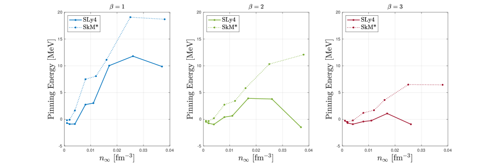
Figure 5: Pinning energies as a function of the neutron sea density $n_{\infty}$, for three values of $\beta$ and for both SLy4 (straight line) and SkM* (dotted line) interactions. The highest density point with SLy4 and $\beta=3$ is absent because it does not satisfy our requirement $\rho^{*}>R_{WS}$ (see section II.2).

In Fig. 5 we show our results for the pinning energy as a function of the neutron sea density $n_{\infty}$ for both SLy4 (straight line) and SkM* (dotted line) interactions. The corresponding numerical values are reported in Tab. 1 and 2.

The value of the pinning energy depends considerably on the value of the interstitial pairing gap, which could be much lower than the bare gap (especially at high densities) due to screening effects. For this reason, we have carried out calculations with $\beta$=2 and 3.

We first point out that with $\beta=3$ and the SLy4 interaction we find $\rho^{*}>R_{WS}$ at the highest density, so the criteria we explained in II.2 are not met. Therefore our method cannot produce a pinning energy value for that point.

Generally, the pinning energy has the same qualitative behavior for both interactions, with SkM* systematically predicting higher values. At the lowest densities, the pinning energy is slightly negative and therefore nuclear pinning is favored. On the other hand, the pinning energy grows considerably with $n_{\infty}$ up to about $n_{\infty}=0.02$ fm^-3, implying that vortex lines are repelled at intermediate densities. At the highest densities, the pinning energy either becomes roughly stable, as in the case of SkM*, or decreases, as for SLy4, where it even becomes negative again for $\beta=$ 2 and 3.

At a given density the pinning energy decreases as a function of $\beta$. This can be understood, considering that the vortex radius (expressed in terms of its coherence length $\xi$) grows with $n_{\infty}$ and with $\beta$, as a larger value of $\beta$ corresponds to a lower pairing field $\Delta$. We have previously seen that the vortex tends to incorporate the nucleus. This costs less energy if the vortex radius is larger, that is, for larger values of $\beta$, because the deformation needed is clearly less significant. The nuclear pinning configuration, while still being not convenient, becomes less unfavorable and the pinning energy decreases considerably with $\beta$.

$n_{\infty}$ [fm-3]	$E_{p}$ [MeV] (SLy4)
	$\beta=1$	$\beta=2$	$\beta=3$
$0.001$	$-0.72$	$-0.48$	$-0.27$
$0.002$	$-0.91$	$-0.75$	$-0.70$
$0.004$	$-0.89$	$-0.97$	$-0.93$
$0.008$	$2.73$	$0.40$	$-0.43$
$0.011$	$3.01$	$0.63$	$-0.26$
$0.017$	$10.00$	$3.90$	$1.06$
$0.026$	$11.78$	$3.77$	$-0.94$
$0.037$	$9.85$	$-1.49$	-

Table 1: Pinning energy and its uncertainty for eight different values of the neutron sea density. We show our results with the SLy4 interaction for the three different values of $\beta$. The highest density point with $\beta=3$ is absent because it does not satisfy our requirement $\rho^{*}>R_{WS}$ (see section II.2).

$n_{\infty}$ [fm-3]	$E_{p}$ [MeV] (SkM*)
	$\beta=1$	$\beta=2$	$\beta=3$
$0.001$	$-0.19$	$-0.30$	$-0.27$
$0.002$	$-0.10$	$-0.35$	$-0.50$
$0.004$	$1.63$	$0.18$	$-0.23$
$0.008$	$7.47$	$2.72$	$1.19$
$0.011$	$8.06$	$3.41$	$1.68$
$0.017$	$11.12$	$5.81$	$3.59$
$0.026$	$19.07$	$10.31$	$6.47$
$0.037$	$18.69$	$12.07$	$6.43$

Table 2: Pinning energy and its uncertainty for eight different values of the neutron sea density. We show our results with the SkM* interaction for the three different values of $\beta$.

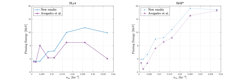
Figure 6: Comparison between our new results (blue dots) on the pinning energy and the results of Paper I Avogadro et al. (2008) (purple triangles). As previously, we show the values as a function of the exterior neutron sea density $n_{\infty}$ for both Sly4 (left) and SkM* (right) interactions and for $\beta=1$.

We carefully checked the dependence of our results on the radius of the Wigner-Seitz cell. We have found that generally, the computed pinning energies tend to stabilize for $R_{WS}$ larger than 35 fm. For each set of parameters, we performed three calculations for $\rho_{WS}$= 38 fm, 40 fm, 42 fm, and the same height ($h_{WS}=40$ fm). The resulting pinning energies differ by less than $\sim 10$ keV at the lowest density we have considered, that is, $n_{\infty}$ = 0.001 fm^-3 and by less than 300 keV at $n_{\infty}$ = 0.017 fm^-3. For a given density, we will report the value averaged over the three boxes. We have found that at the two largest computed densities, namely $n_{\infty}$ = 0.026 fm^-3 and $n_{\infty}$ = 0.037 fm^-3, the convergence pattern is more complicated, and we considered also larger values of $R_{WS}$, up to 48 fm. The HFB self-consistent process for the NP configurations can lead to two solutions having a different pairing and density spatial dependence, according to the box radius, and differing from each other by about 1.5 MeV. For these two densities, the boxes displaying the deepest minima were selected, in keeping with the variational nature of our approach. The resulting uncertainty on the pinning energy is equal to about 500 keV.

We conclude this section comparing our results with those reported in Paper I in Fig. 6. The pinning energies computed with the SLy4 and the SkM* interaction are shown in the left and right panel respectively. Only the value $\beta=1$ was considered in Paper I. The results obtained for the SkM* interaction are similar, aside from a sharp fall of the pinning energy in the second density zone. On the other hand, for SLy4 the situation is rather different: the new results are more regular and grow monotonously with $n_{\infty}$, while the previous ones present a distinct oscillatory behavior. Quantitatively, the difference with the results of Paper I is substantial at the largest densities, where the present pinning energies are larger by 5-10 MeV.

To study these differences in more detail, in Fig. 7 we consider first the effect of proton deformation and of Coulomb exchange, which were not taken into account in Paper I. Proton deformation decreases the energy of the NP configuration; on the other hand, it does not affect the Nu configuration, in which we consider a spherical, closed shell nucleus. As a consequence (see Eq. (7)) the pinning energy decreases, and therefore this effect cannot explain why the pinning energies are larger than those calculated in Paper I. In any case, one sees in Fig. 7 (see in particular the inset) that this effect is significant only for the largest densities, where it amounts to about 600-700 KeV. Neglecting deformation but including Coulomb exchange, on the other hand, decreases the pinning energy by at most about 100 keV.

We then conclude that the differences with Paper I must be related to the improvements in the computational algorithms. This point is further considered in Appendix B.

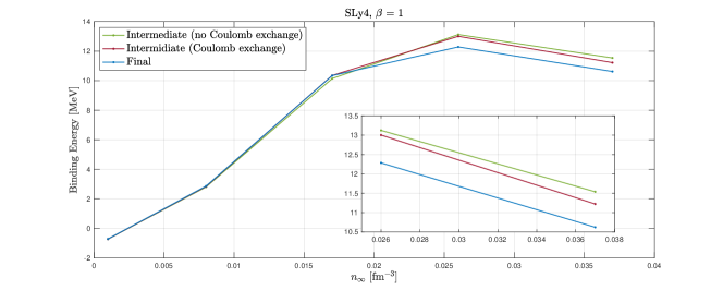
Figure 7: The pinning energy calculated with the SLy4 interaction for $\beta=1$ as a function of neutron density, already shown in Fig. 5. Our results (blue line) are compared with the one obtained neglecting both proton deformation and Coulomb exchange (green line) or neglecting only proton deformation (red line). The results obtained at the highest densities are shown in more detail in the inset.

III.3 Mesoscopic pinning forces

The pinning energy contains information about the microscopic interaction between a vortex and a single nucleus. Nonetheless, inner crust vortices are much longer than the lattice spacing and are expected to interact with many pinning sites (Seveso et al., 2016; Antonelli and Haskell, 2020), giving rise to pinning at the mesoscopic scale (an intermediate scale in between the lattice spacing and the typical distance between two vortices in a pulsar).

Seveso et al. (2016) found a simple prescription to estimate the mesoscopic pinning force per unit length $f_{L}$ acting on a vortex segment of length $L$, which is a better representative of the vortex-lattice interaction than the single-nucleus pinning energy, see the discussion in (Antonelli and Haskell, 2020). They found an analytic approximation where the force per unit length $f_{L}=f_{L}(E_{p},\,R_{WS},L)$ is a function of the pinning energy $E_{p}$ and the dimension of the WS cell $R_{WS}$. This function depends also on the parameter $L$, the typical length over which a vortex filament in the inner crust could be approximated as straight. Finally, the estimate of $f_{L}(E_{p},\,R_{WS},L)$ also depends on the geometrical properties of the lattice and on whether there is nuclear or interstitial pinning. However, the authors found that this distinction has a low impact on the pinning strength results, a result that is confirmed also by the dynamical simulations of an ensemble of vortices in complex pinning landscapes performed in Antonelli and Haskell (2020); Link and Levin (2022).

By following the procedure in Seveso et al. (2016), we can calculate new estimates for the typical pinning force for three different values of the parameter $L$ that defines the scale on which a vortex can be considered straight ($L=1000,2500,5000\;R_{WS}$, see Seveso et al. (2016)). Our results are shown in Fig. 8. We plot the absolute value of the force per unit length; where it is marked with dots, it is repulsive, otherwise, it is attractive where marked by circles. The mesoscopic pinning force values are of the same order of magnitude as the results of Seveso et al. (2016): the force per unit length ranges from $\sim 10^{13}$ dyn/cm up to $\sim 10^{16}$ dyn/cm.

While most of the remarks present in Seveso et al. (2016) are valid for our results too, we briefly underline the following aspect. The force decreases as the vortex length increases. Note that for an infinitely long and rigid vortex, the pinning force should vanish. In fact, if the vortex were to move, the number of nuclei with which it interacts would not changeJones (1991); Seveso et al. (2016).

We can also compare our findings with the results of Wlazłowski et al. (2016), which are obtained through a different method. In particular, from inset (b) of Fig. 3 of their work, we can see that they found a repulsive force of the order of $\sim 0.5$ MeV/fm when the vortex-nucleus distance is approximately 20 fm; after conversion to appropriate units, this is broadly consistent with our results.

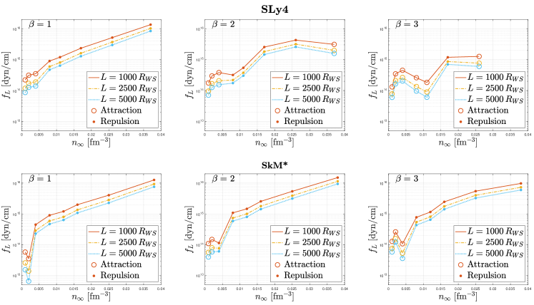
Figure 8: Absolute value of the pinning force per unit length as a function of the neutron sea density $n_{\infty}$, for both SLy4 (upper half) and SkM* (lower half) interactions. Where it is attractive, we used a hollow circle, while where it is repulsive we used a dot. The values have been found using the prescription in Seveso et al. (2016) for three different maximum-straight lengths $L=1000$ (straight line), 2500 (line-dot), and 5000 (dotted line) $R_{WS}$. We plotted the results for the three different values of $\beta$ used. As for the corresponding pinning energy, the highest density point with SLy4 and $\beta=3$ is absent because it does not satisfy our requirement $\rho^{*}>R_{WS}$ (see section II.2).

IV Conclusions

Microscopic pinning energies are a crucial ingredient in the dynamics of vortex-mediated pulsar glitches. The stronger the pinning of a vortex line, the larger the amount of angular momentum that can be stored in the inner crust in the form of a persistent (dissipationless) neutron current, which can then be potentially released in a glitch Antonelli et al. (2022).

Most of the past estimates of the pinning energies relied on a classical or semiclassical picture and had to use significant approximations to describe nuclei. Working in the microscopic HFB framework solves these problems, as was done in Paper I Avogadro et al. (2008). We have expanded and improved the latter work in four respects: we have i) allowed for the axial deformation of protons; ii) included the effect of the Coulomb exchange; iii) considered, although schematically, the effects of the screening of the pairing interaction; and iv) improved the numerical treatment giving special attention to the convergence of our results. Based on these improvements, we found new and more reliable results on the pinning energy.

Our results show that nuclei attract vortices for the lower external neutron sea densities, while the situation is the opposite at higher densities unless the pairing gap is strongly screened. From our estimates of the pinning binding energy, we then extracted the typical force per unit length acting on a vortex, consistently with the procedure developed in Seveso et al. (2016). This force defines a theoretical upper limit on the depinning threshold Antonelli and Haskell (2020) and, accordingly, an upper limit on the glitch amplitude in general relativity Antonelli et al. (2018). Therefore, in Sec. III.3 we have checked that our mesoscopic pinning forces are sufficiently large to be consistent with observations of giant glitches in the Vela pulsar.

Appendix A Numerical details

Within the HF approximation, one can obtain an explicit expression for the self-consistent potential of the Skyrme potential

$$h(\mathbf{x})=-\nabla\frac{\hbar^{2}}{2m^{*}_{q}(\mathbf{x})}\nabla+U_{q}(\mathbf{x})+\delta_{q,p}V_{C}$$ (11)

where $q$ can stand for $p$ (protons) or $n$ (neutrons). Remembering that $n_{q}$ and $\tau_{q}$ are the density and the kinetic density of either protons or neutrons, and that $n=n_{p}+n_{n}$ and $\tau=\tau_{p}+\tau_{n}$, we write the terms in (11) following Chabanat et al. (1997). The effective mass $m^{*}_{q}$ is

$$\frac{\hbar^{2}}{2m^{*}_{q}(\mathbf{x})}=\frac{\hbar^{2}}{2m_{q}}+\frac{1}{8}\bigg{[}t_{1}(2+x_{1})+t_{2}(2+x_{2})\bigg{]}n(\mathbf{x})$$ (12)

$$-\frac{1}{8}\bigg{[}t_{1}(1+2x_{1})+t_{2}(1+2x_{2})\bigg{]}n_{q}(\mathbf{x})$$

the self-consistent potential $U_{q}$ reads

$$\begin{split}U_{q}(\mathbf{x})&=\frac{1}{2}t_{0}\bigg{[}(2+x_{0})n+(1+2x_{0})n_{q}\bigg{]}\\ &+\frac{1}{24}t_{3}\bigg{\{}(2+x_{3})(2+\alpha)n^{\alpha+1}-\\ &(2x_{3}+1)\left[2n^{\alpha}n_{q}+\alpha n^{\alpha-1}(n_{p}^{2}+n_{n}^{2})\right]\bigg{\}}\\ &+\frac{1}{8}\bigg{[}t_{1}(2+x_{1})+t_{2}(2+x_{2})\bigg{]}\tau+\\ &\frac{1}{8}\bigg{[}t_{2}(1+2x_{2})-t_{1}(1+2x_{1})\bigg{]}\tau_{q}\\ &+\frac{1}{16}\bigg{[}t_{2}(2+x_{2})-3t_{1}(2+x_{1})\bigg{]}\nabla^{2}n\\ &+\frac{1}{16}\bigg{[}t_{2}(1+2x_{2})+3t_{1}(1+2x_{1})\bigg{]}\nabla^{2}n_{q}\\ \end{split}$$ (13)

Lastly, the Coulomb potential, with the Slater approximation for the exchange part, reads

$$V_{C}(\mathbf{x})=e^{2}\left(\int\frac{n_{p}(\mathbf{x}^{\prime})\mathrm{d}_{3}x^{\prime}}{|\mathbf{x}-\mathbf{x^{\prime}}|}-\left(\frac{3}{\pi}\right)^{\frac{1}{3}}n_{p}(\mathbf{x})^{\frac{1}{3}}\right)$$ (14)

In the code, we neglect the spin-orbit interaction, taking into account the spin simply with a degeneracy factor $g=2$.

Each term of the potentials contributes to a term of the energy density of the system $\mathcal{H_{HF}}(\mathbf{x})$, which in turn is subdivided into different components

$$\mathcal{H_{HF}}=\mathcal{K}+\mathcal{H}_{0}+\mathcal{H}_{3}+\mathcal{H}_{eff}+\mathcal{H}_{fin}+\mathcal{H}_{C}$$ (15)

where each term reads

$$\begin{split}\mathcal{K}&=\frac{\hbar^{2}}{2m}\tau\\ \mathcal{H}_{0}&=\frac{1}{4}t_{0}\bigg{[}(2+x_{0})n^{2}-(2x_{0}+1)(n_{p}^{2}+n^{2}_{n})\bigg{]}\\ \mathcal{H}_{3}&=\frac{1}{24}t_{3}n^{\alpha}\bigg{[}(2+x_{3})n^{2}-(2x_{3}+1)(n^{2}_{p}+n^{2}_{n})\bigg{]}\\ \mathcal{H}_{eff}&=\frac{1}{8}\bigg{[}t_{1}(2+x_{1})+t_{2}(2+x_{2})\bigg{]}\tau n\\ &+\frac{1}{8}\bigg{[}t_{2}(2x_{2}+1)-t_{1}(2x_{1}+1)\bigg{]}(\tau_{p}n_{p}+\tau_{n}n_{n})\\ \mathcal{H}_{fin}&=\frac{1}{32}\bigg{[}3t_{1}(2+x_{1})-t2(2+x_{2})\bigg{]}\left(\nabla n\right)^{2}\\ &-\frac{1}{32}\biggl{[}3t_{1}(2x_{1}+1)+3t_{2}(2x_{2}+1)\biggr{]}\left[\left(\nabla n_{p}\right)^{2}+\left(\nabla n_{n}\right)^{2}\right]\\ \mathcal{H}_{C}&=e^{2}\left(\frac{n_{p}}{2}\int\frac{n_{p}(\mathbf{x}^{\prime})\mathrm{d}_{3}x^{\prime}}{|\mathbf{x}-\mathbf{x^{\prime}}|}-\frac{3}{4}\left(\frac{3}{\pi}\right)^{\frac{1}{3}}n_{p}(\mathbf{x})^{\frac{4}{3}}\right)\end{split}$$ (16)

We solve (1) in a cylindrical box with height $h_{box}$ and radius $\rho_{box}$. We search for a solution expanded on a single-particle basis so that the amplitudes $u_{qm}(\rho,z,\varphi)$ and $v_{qm}(\rho,z,\varphi)$ for the quasi-particle level $q$ with projection of angular momentum along the $z$-axis $m$ are

$$\begin{split}u_{qm}(\rho,z,\varphi)&=\displaystyle\sum_{nl}U_{qm}^{nl}f_{nm}(\rho)g_{l}(z)e^{im\varphi}\\ v_{qm}(\rho,z,\varphi)&=\displaystyle\sum_{nl}V_{qm}^{nl}f_{nm-\nu}(\rho)g_{l}(z)e^{i(m-\nu)\varphi}\\ \end{split}$$ (17)

On the $\rho$ axis, functions $f_{nm}(\rho)$ are the solution of the Schrödinger equation for free particles

$$-\frac{\hbar^{2}}{2m_{0}}\left(\frac{1}{\rho}\partialderivative{\rho}\left(\rho\partialderivative{\rho}\right)+\frac{m^{2}}{\rho^{2}}\right)f_{nm}(\rho)=e_{nm}f_{nm}(\rho)$$ (18)

where $m_{0}$ is the bare nucleon mass and the index $n$ is the number of nodes of function $f_{nm}(\rho)$ on the $\rho$ axis.

On the $z$ axis, functions $g_{l}(z)$ are normalized plane waves

$$g_{l}(z)=\sqrt{\frac{2}{h_{box}}}\sin\left(k_{l}\left(z+\frac{h_{box}}{2}\right)\right),\;k_{l}=\frac{\pi}{h_{box}},\frac{2\pi}{h_{box}},\dots$$ (19)

so that we have

$$\begin{split}-\frac{\hbar^{2}}{2m_{0}}\left(\partialderivative[2]{z}+\frac{1}{\rho}\partialderivative[2]{\varphi}+\frac{1}{\rho}\partialderivative{\rho}\left(\rho\partialderivative{\rho}\right)\right)&f_{nm}(\rho)g_{l}(z)e^{im\varphi}=\\ \left(e_{nm}+\frac{\hbar^{2}k_{l}^{2}}{2m_{0}}\right)&f_{nm}(\rho)g_{l}(z)e^{im\varphi}\end{split}$$ (20)

As for the boundary condition, each single-particle function vanishes at the edge of the box.

To solve (1), we project it onto generic basis states $\ket{m_{i},n_{i},l_{i}}=\ket{\alpha_{i}}$. Therefore our system of equations becomes, in matrix form

$$\matrixquantity(\matrixelement{\alpha_{2}}{h-\lambda}{\alpha_{1}}&\matrixelement{\alpha_{2}}{\Delta}{\alpha_{1}}\\ \matrixelement{\alpha_{2}}{\Delta^{*}}{\alpha_{1}}&-\matrixelement{\alpha_{2}}{h-\lambda}{\alpha_{1}})$$ (21)

Since $h$ depends only on the density, and the density does not depend on the azimuthal angle $\varphi$, it holds

$$\matrixelement{m_{2},n_{2},l_{2}}{h}{m_{1},n_{1},l_{1}}=\delta_{m_{1},m_{2}}\matrixelement{n_{2},l_{2}}{h}{n_{1},l_{1}}$$ (22)

On the other hand, $\Delta=\Delta(\rho,z)e^{i\nu\varphi}$. It follows

$$\matrixelement{m_{2},n_{2},l_{2}}{\Delta}{m_{1},n_{1},l_{1}}=\delta_{m_{1},m_{2}+\nu}\matrixelement{n_{2},l_{2}}{\Delta(\rho,z)}{n_{1},l_{1}}$$ (23)

We can now rewrite (1) explicitly. From (11) and (5), we find

$$\begin{cases}\displaystyle\sum_{n_{2}l_{2}}\left(h^{m}_{n_{1}l_{1}n_{2}l_{2}}-\lambda\right)U^{qm}_{n_{2}l_{2}}+\Delta^{m}_{n_{1}l_{1}n_{2}l_{2}}V^{qm}_{n_{2}l_{2}}&=E^{qm}U^{qm}_{n_{1}l_{1}}\\ \displaystyle\sum_{n_{2}l_{2}}\Delta^{m}_{n_{1}l_{1}n_{2}l_{2}}U^{qm}_{n_{2}l_{2}}-\left(h^{m}_{n_{1}l_{1}n_{2}l_{2}}-\lambda\right)V^{qm}_{n_{2}l_{2}}&=E^{qm}V^{qm}_{n_{1}l_{1}}\end{cases}$$ (24)

where

$$h^{m}_{n_{1}l_{1}n_{2}l_{2}} = 2\pi\int_{0}^{h_{box}}2\mathrm{d}z\;\int_{0}^{\rho_{box}}\rho\,\mathrm{d}\rho\Bigg{\{}f_{n_{2}m}(\rho)g_{{l_{2}}}(z)\left(U(\rho,z)+\left(\frac{m_{0}}{m^{*}(\rho,z)}\right)\left(e_{n_{1}m}+\frac{\hbar^{2}k_{l_{1}}^{2}}{2m_{0}}\right)-\lambda\right)f_{n_{1}m}(\rho)g_{{l_{1}}}(z)$$

$$+ f_{n_{2}m}(\rho)g_{{l_{2}}}(z)\left(\partialderivative{\rho}\left(\frac{\hbar^{2}}{2m^{*}(\rho,z)}\right)\cdot\partialderivative{f_{n_{1}m}(\rho)}{\rho}\right)g_{{l_{1}}}(z)+f_{n_{2}m}(\rho)g_{{l_{2}}}(z)\left(\partialderivative{z}\left(\frac{\hbar^{2}}{2m^{*}(\rho,z)}\right)\cdot\partialderivative{g_{{l_{1}}}(z)}{z}\right)f_{n_{1}m}(\rho)\Bigg{\}}$$

and

$$\Delta^{m}_{n_{1}l_{1}n_{2}l_{2}}=2\pi\int_{0}^{h_{box}}2\mathrm{d}z\;\int_{0}^{\rho_{box}}\rho\,\mathrm{d}\rho\left(f_{n_{2}m-\nu}(\rho)g_{{l_{2}}}(z)\Delta(\rho,z)f_{n_{1}m}(\rho)g_{{l_{1}}}(z)\right)$$ (26)

Since protons and neutrons feel different self-consistent potentials (13), they give rise to two systems (24). From the solution of such systems, we then compute new densities, which we can use to write a new set of equations (24). This iterative process stops once the relative energy difference between subsequent iterations is lower than an appropriate value. Since protons are confined in the nucleus, the dimension of their box is smaller, fixed at 15 fm: so that it’s big enough to contain all the protons but small enough to shorten the calculation times. Finally, we do not consider proton pairing.

Appendix B Numerical Test

We test the accuracy of our axially deformed HFB code by applying it to the spherical nucleus ⁴⁰Ca and comparing the results with the those obtained with the spherical code hfbcs-qrpa Colò and Roca-Maza (2021). For this test, we use the SLy4 interaction without the spin-orbit terms.

In Table 3 we show the total energy, divided among its contributions, as listed in (16); the only exception being $E_{12}$, which is defined as $E_{12}=E_{fin}+E_{eff}$. The relative difference between the hfbcs-qrpa results and our program amount to 0.1-0.3%.

In Table 6 we list the single-particle energy levels of neutrons and protons. We see that the present code reproduces the degeneracy of the Levels with the same values of the angular momentum $l$ within a few keVs, while deviations of the order of 100 keV are found in the original code.

Table 3: All contributions to the total energy ($E_{tot}$). Values are expressed in MeV. $\delta E$ is the relative energy difference (in percentage) between each value and the standard HF equivalent. We divided the energy in its main contributions, as in (16), except for $E_{12}$, which is defined as $E_{12}=E_{fin}+E_{eff}$. The interaction used was SLy4 and the spin-orbit terms were neglected, as well as the Coulomb exchange potential.

	Ref. Colò and Roca-Maza (2021)	Present work	$\delta E(\%)$
$K$	$640.21$	$638.93$	0.1
$E_{0}$	$-3716.80$	$-3707.01$	0.3
$E_{3}$	$2398.00$	$-2391.19$	0.3
$E_{12}$	$279.59$	$278.83$	0.3
$E_{C}$	$78.94$	$78.72$	$0.3$
$E_{tot}$	$-320.03$	$-319.33$	$0.2$

		Neutrons		Protons
		Ref. Colò and Roca-Maza (2021)	Present work	Ref. Colò and Roca-Maza (2021)	Present work
2s	$l_{z}=0$	$-16.95$	$-16.889$	$-9.48$	$-9.459$
	$l_{z}=2$	$-18.85$	$-18.785$	$-11.40$	$-11.361$
	$l_{z}=1$	$-18.85$	$-18.786$	$-11.40$	$-11.362$
1d	$l_{z}=0$	$-18.85$	$-18.789$	$-11.40$	$-11.371$
	$l_{z}=-1$	$-18.85$	$-18.786$	$-11.40$	$-11.362$
	$l_{z}=-2$	$-18.85$	$-18.785$	$-11.40$	$-11.361$
	$l_{z}=1$	$-33.21$	$-33.184$	$-25.29$	$-25.282$
1p	$l_{z}=0$	$-33.21$	$-33.182$	$-25.29$	$-25.277$
	$l_{z}=-1$	$-33.21$	$-33.184$	$-25.29$	$-25.282$
1s	$l_{z}=0$	$-47.82$	$-47.799$	$-39.36$	$-39.356$

Table 4: Energies of each single particle level, both for protons and neutrons, expressed in MeV.

Appendix C $\rho^{*}$ criterion

We show here the values of the critical distance $\rho^{*}=R_{N}+\xi$ (see eq. (9)) for the two adopted Skyrme parametrizations and for three values of the gap-reduction factor $\beta$.

We observe that the value of $\rho^{*}$ is mostly determined by the pairing gap. As a consequence, $\rho^{*}$ has a minimum at intermediate densities, where the pairing gap reaches its maximum value.

$n_{\infty}$ [fm-3]	$R_{WS}$ [fm]	$\rho^{*}$ [fm] (SLy4)
		$\beta=1$	$\beta=2$	$\beta=3$
$0.001$	$43.7$	$11.8$	$16.3$	$21.0$
$0.002$	$41.5$	$11.9$	$16.0$	$20.0$
$0.004$	$38.8$	$11.4$	$14.2$	$16.7$
$0.008$	$33.7$	$11.1$	$13.1$	$14.9$
$0.011$	$31.8$	$11.2$	$13.1$	$14.7$
$0.017$	$28.9$	$11.6$	$13.6$	$15.3$
$0.026$	$25.6$	$12.5$	$15.0$	$17.2$
$0.037$	$21.4$	$14.5$	$18.5$	$21.7$

Table 5: Critical distance $\rho^{*}$ from our calculations with the SLy4 Skyrme parametrization. For $\beta=3$, the value of $\rho^{*}$ is comparable to the dimension of the WS cell; therefore our method cannot estimate the pinning energy for this case.

$n_{\infty}$ [fm-3]	$R_{WS}$ [fm]	$\rho^{*}$ [fm] (SkM*)
		$\beta=1$	$\beta=2$	$\beta=3$
$0.001$	$43.7$	$11.3$	$15.9$	$20.6$
$0.002$	$41.5$	$11.7$	$16.3$	$21.0$
$0.004$	$38.8$	$11.5$	$13.9$	$19.7$
$0.008$	$33.7$	$10.7$	$12.7$	$14.2$
$0.011$	$31.8$	$10.7$	$12.4$	$13.9$
$0.017$	$28.9$	$10.7$	$12.4$	$13.8$
$0.025$	$25.6$	$11.2$	$12.9$	$14.3$
$0.038$	$21.4$	$12.3$	$14.0$	$14.0$

Table 6: Critical distance $\rho^{*}$ from our calculations with the SkM* Skyrme parametrization.

References

- Fuentes, J. R. et al. (2017) Fuentes, J. R., Espinoza, C. M., Reisenegger, A., Shaw, B., Stappers, B. W., and Lyne, A. G., “The glitch activity of neutron stars,” A&A 608, A131 (2017).
- Baym et al. (1969) Gordon Baym, Christopher Pethick, David Pines, and Malvin Ruderman, “Spin Up in Neutron Stars : The Future of the Vela Pulsar,” Nature 224, 872–874 (1969).
- Haskell and Melatos (2015) Brynmor Haskell and Andrew Melatos, “Models of pulsar glitches,” International Journal of Modern Physics D 24, 1530008 (2015), arXiv:1502.07062 [astro-ph.SR] .
- Antonelli et al. (2022) M. Antonelli, A. Montoli, and P.M. Pizzochero, Insights Into the Physics of Neutron Star Interiors from Pulsar Glitches (World Scientific, Singapore, 2022) pp. 219–281, arXiv:2301.12769 [astro-ph.HE] .
- Chamel and Haensel (2008) Nicolas Chamel and Pawel Haensel, “Physics of Neutron Star Crusts,” Living Reviews in Relativity 11, 10 (2008), arXiv:0812.3955 [astro-ph] .
- Haensel et al. (2007) P. Haensel, A. Y. Potekhin, and D. G. Yakovlev, Neutron stars 1: Equation of state and structure, Vol. 326 (Springer, New York, USA, 2007).
- Negele and Vautherin (1973) J.W. Negele and D. Vautherin, “Neutron star matter at sub-nuclear densities,” Nuclear Physics A 207, 298–320 (1973).
- Pizzochero et al. (2002) P.M. Pizzochero, F. Barranco, Vigezzi E., and Broglia R.A., “Nuclear impurities in the superfluid crust of neutron stars: quantum calculation and observable effects on the cooling,” Astrophys. J. 569, 381 (2002).
- Sandulescu et al. (2004) N. Sandulescu, N.V. Giai, and R.J. Liotta, “Superfluid properties of the inner crust of neutron stars,” Phys. Rev. C 69, 045802 (2004).
- Baldo et al. (2007) M. Baldo, E. Saperstein, and S. Tolokonnikov, “A realistic model of superfluidity in the neutron star inner crust,” Eur. Phys. Jou. A 32, 97 (2007).
- Grill et al. (2011) F. Grill, J. Margueron, and N. Sandulescu, “Cluster structure of the inner crust of neutron stars in the hartree-fock-bogoliubov approach,” Phys. Rev. C 84, 065807 (2011).
- Pastore et al. (2011) A. Pastore, S. Baroni, and C. Losa, “Superfluid properties of the inner crust of neutron stars,” Phys. Rev. C 84, 065807 (2011).
- Mondal et al. (2020) C. Mondal, X. Viñas, M. Centelles, and J. N. De, “Structure and composition of the inner crust of neutron stars from Gogny interactions,” Phys. Rev. C 102, 015802 (2020), arXiv:2003.03338 [nucl-th] .
- Shelley and Pastore (2021) M. Shelley and A. Pastore, “Systematic analysis of inner crust composition using the extended thomas-fermi approximation with pairing correlations,” Phys. Rev. C 103, 035807 (2021).
- Sedrakian and Clark (2019) Armen Sedrakian and John W. Clark, “Superfluidity in nuclear systems and neutron stars,” European Physical Journal A 55, 167 (2019), arXiv:1802.00017 [nucl-th] .
- Feynman (1998) R.P. Feynman, Statistical Mechanics: A Set Of Lectures, Advanced Books Classics (Avalon Publishing, 1998).
- Antonelli et al. (2018) M. Antonelli, A. Montoli, and P. M. Pizzochero, “Effects of general relativity on glitch amplitudes and pulsar mass upper bounds,” Mon. Not. Roy. Astr. Soc. 475, 5403–5416 (2018), arXiv:1710.05879 [astro-ph.HE] .
- Anderson and Itoh (1975) P. W. Anderson and N. Itoh, “Pulsar glitches and restlessness as a hard superfluidity phenomenon,” Nature 256, 25–27 (1975).
- Warszawski and Melatos (2013) L. Warszawski and A. Melatos, “Knock-on processes in superfluid vortex avalanches and pulsar glitch statistics,” Mon. Not. Roy. Astr. Soc. 428, 1911–1926 (2013), arXiv:1210.2203 [astro-ph.HE] .
- Glampedakis and Andersson (2009) Kostas Glampedakis and Nils Andersson, “Hydrodynamical Trigger Mechanism for Pulsar Glitches,” Phys. Rev. Lett. 102, 141101 (2009), arXiv:0806.3664 [astro-ph] .
- Khomenko et al. (2019) V. Khomenko, M. Antonelli, and B. Haskell, “Hydrodynamical instabilities in the superfluid interior of neutron stars with background flows between the components,” Phys. Rev. D 100, 123002 (2019), arXiv:1906.05177 [astro-ph.HE] .
- Andersson et al. (2012) N. Andersson, K. Glampedakis, W. C. G. Ho, and C. M. Espinoza, “Pulsar Glitches: The Crust is not Enough,” Phys. Rev. Lett. 109, 241103 (2012), arXiv:1207.0633 [astro-ph.SR] .
- Chamel (2013) N. Chamel, “Crustal Entrainment and Pulsar Glitches,” Phys. Rev. Lett. 110, 011101 (2013), arXiv:1210.8177 [astro-ph.HE] .
- Montoli et al. (2021) A. Montoli, M. Antonelli, B. Haskell, and P. Pizzochero, “Statistical Estimates of the Pulsar Glitch Activity,” Universe 7, 8 (2021), arXiv:2012.01539 [astro-ph.HE] .
- Sauls et al. (2020) J. A. Sauls, N. Chamel, and M. A. Alpar, “Superfluidity in Disordered Neutron Stars Crusts,” arXiv e-prints , arXiv:2001.09959 (2020), arXiv:2001.09959 [astro-ph.HE] .
- Antonelli and Haskell (2020) M. Antonelli and B. Haskell, “Superfluid vortex-mediated mutual friction in non-homogeneous neutron star interiors,” Mon. Not. Roy. Astr. Soc. 499, 3690–3705 (2020), arXiv:2007.11720 [astro-ph.HE] .
- Donati and Pizzochero (2006) Paola Donati and Pierre M. Pizzochero, “Realistic energies for vortex pinning in intermediate-density neutron star matter,” Physics Letters B 640, 74–81 (2006).
- Avogadro et al. (2008) P. Avogadro, F. Barranco, R. A. Broglia, and E. Vigezzi, “Vortex nucleus interaction in the inner crust of neutron stars,” Nucl. Phys. A 811, 378–412 (2008), arXiv:0804.1765 [astro-ph] .
- Epstein and Baym (1988) Richard I. Epstein and Gordon Baym, “Vortex Pinning in Neutron Stars,” Astro. Phys. Jour. 328, 680 (1988).
- Donati and Pizzochero (2004) Paola Donati and Pierre M. Pizzochero, “Fully consistent semi-classical treatment of vortex-nucleus interaction in rotating neutron stars,” Nucl. Phys. A 742, 363–379 (2004).
- Avogadro et al. (2007) P. Avogadro, F. Barranco, R. A. Broglia, and E. Vigezzi, “Quantum calculation of vortices in the inner crust of neutron stars,” Phys. Rev. C 78, 012805(R) (2007).
- Seveso et al. (2016) S. Seveso, P. M. Pizzochero, F. Grill, and B. Haskell, “Mesoscopic pinning forces in neutron star crusts,” Mon. Not. Roy. Astr. Soc. 455, 3952–3967 (2016).
- Wlazłowski et al. (2016) Gabriel Wlazłowski, Kazuyuki Sekizawa, Piotr Magierski, Aurel Bulgac, and Michael McNeil Forbes, “Vortex pinning and dynamics in the neutron star crust,” Phys. Rev. Lett. 117, 232701 (2016).
- Bulgac et al. (2013) A. Bulgac, M.M. Forbes, and R. Sharma, “Strength of the vortex-pinning interaction from real-time dynamics,” Phys. Rev. Lett. 110, 241102 (2013).
- Link (2009) B. Link, “Dynamics of quantum vorticity in a random potential,” Phys. Rev. Lett. 102, 131101 (2009).
- Pecak et al. (2021) Daniel Pecak, Nicolas Chamel, Piotr Magierski, and Gabriel Wlazlowski, “Properties of a quantum vortex in neutron matter at finite temperatures,” Phys. Rev. C 104, 055801 (2021).
- Chabanat et al. (1997) E. Chabanat, P. Bonche, P. Haensel, J. Meyer, and R. Schaeffer, “A Skyrme parametrization from subnuclear to neutron star densities,” Nucl. Phys. A 627, 710–746 (1997).
- Garrido et al. (1999) E. Garrido, P. Sarriguren, E. Moya de Guerra, and P. Schuck, “Effective density-dependent pairing forces in the T=1 and T=0 channels,” Phys. Rev. C 60, 064312 (1999), arXiv:nucl-th/9909026 [nucl-th] .
- Ramanan and Urban (2021) S. Ramanan and M. Urban, “Pairing in Pure Neutron Matter,” Eur. Phys. Jour. Spec. Top. 230, 567 (2021).
- Gandolfi et al. (2022) S. Gandolfi, G Palkanoglou, J. Carlson, A. Gezerlis, and K. E. Schmidt, “The Pairing Gap,” Condens. Matter 7, 19 (2022).
- Gygi and Schlüter (1991) François Gygi and Michael Schlüter, “Self-consistent electronic structure of a vortex line in a type-II superconductor,” Phys Rev. B 43, 7609–7621 (1991).
- Avogadro et al. (2012) P. Avogadro, F. Barranco, R. A. Broglia, and E. Vigezzi, Nutron Star Crust, edited by C. Bertulani and J. Piekarewicz (Nova Science Publishers, New York, 2012) pp. 309–328.
- Pearson and Chamel (2022) J. M. Pearson and N. Chamel, “Unified equations of state for cold nonaccreting neutron stars with brussels-montreal functionals. iii. inclusion of microscopic corrections to pasta phases,” Phys. Rev. C 105, 015803 (2022).
- Link and Levin (2022) Bennett Link and Yuri Levin, “Vortex Pinning in Neutron Stars, Slipstick Dynamics, and the Origin of Spin Glitches,” Astro. Phys. Jour. 941, 148 (2022), arXiv:2208.11494 [astro-ph.HE] .
- Jones (1991) P. B. Jones, “Rotation of the Neutron-Drip Superfluid in Pulsars: The Interaction and Pinning of Vortices,” Astro. Phys. Jour. 373, 208 (1991).
- Colò and Roca-Maza (2021) Gianluca Colò and Xavier Roca-Maza, “User guide for the hfbcs-qrpa(v1) code,” (2021), arXiv:2102.06562 [nucl-th] .