Age of Incorrect Information With Hybrid ARQ Under a Resource Constraint for $N$-ary Symmetric Markov Sources

Abstract

The Age of Incorrect Information (AoII) is a recently proposed metric for real-time remote monitoring systems. In particular, AoII measures the time the information at the monitor is incorrect, weighted by the magnitude of this incorrectness, thereby combining the notions of freshness and distortion. This paper addresses the definition of an AoII-optimal transmission policy in a discrete-time communication scheme with a resource constraint and a hybrid automatic repeat request (HARQ) protocol. Considering an $N$-ary symmetric Markov source, the problem is formulated as an infinite-horizon average-cost constrained Markov decision process (CMDP). The source model is characterized by the cardinality of the state space and the probability of staying at the same state. Interestingly, it is proved that under some conditions, the optimal transmission policy is to never transmit. This reveals that there exists a region of the source dynamics where communication is inadequate in reducing the AoII. Elsewhere, there exists an optimal transmission policy, which is a randomized mixture of two discrete threshold-based policies that randomize at one state. The optimal threshold and the randomization component are derived analytically. Numerical results illustrate the impact of source dynamics, channel conditions, and resource constraints on the average AoII.

I Introduction

The technological advancements in sensor and monitoring devices, together with the development and widespread utilization of the 5G cellular networks, lead to the continuous emergence of new applications, whose principal element is the real-time monitoring of remote sources. The increasing list of examples includes autonomous driving, real-time video feedback, anomaly detection in critical infrastructures, remote surgery, emerging applications in augmented reality networks and haptic communications. In such applications, timely delivery of information is fundamental.

It is well understood that, while low-latency networks are necessary, they are insufficient to guarantee timely operation [bib:aoi]. This has led to the rising interest in the Age of Information (AoI) metrics to analyze and design such real-time applications. This new family of communication metrics captures the end-to-end latency in remote monitoring systems. Principally, the instantaneous AoI at time $t$ is defined as the difference $t\!-\!u_{t}\!\geq\!0$, where $u_{t}$ is the generation time of the most recently successfully decoded packet. Therefore, AoI quantifies the freshness of the information content of a packet and the importance of updating the monitor with fresh information due to excess ageing.

The most important contribution of AoI has been the opening of a new perspective in the analysis and design of task-oriented communication systems. Since its introduction in [bib:aoi], AoI has attracted the interest of researchers and engineers from many fields [bib:aoi_survey]. Nevertheless, a shortcoming of the conventional AoI metric was shortly noticed. In particular, AoI quantifies the information freshness but omits the dynamics of the data source. For example, consider a source that changes rapidly and another that changes slowly. The packets that were generated at the same time from the two sources will have the same AoI, but obviously, the packet from the rapidly-changing source is less accurate. The initial reaction of the research community pointed towards the generalization of the conventional AoI metric with non-linear age functions [bib:nonlinear_Kosta, bib:nonlinear_Sun, bib:value], or even arbitrary non-decreasing functions [bib:updatewait]. In [bib:stamatakis], the authors studied a system where the source alternates between slow and rapid states, taking into account the time that the monitor knows the wrong state.

From another perspective, a rather expected yet very interesting observation has been made, i.e., minimizing the AoI is not necessarily equivalent to minimizing the real-time estimation error. Particularly, if the sampling times are independent of the observed source, it can be shown that the mean-squared estimation error is an increasing function of the AoI. However, if the sampling times depend on the history of the source, the estimation error is not necessarily minimized with the AoI. This was shown to happen even in the simplest signals [bib:wiener, bib:ornstein], and similar results were derived for the real-time state estimation error of feedback control systems [bib:state1, bib:state2].

Apparently, the conventional AoI ignores the content of the communicated data. On the other hand, the traditional metrics of error ignore the amount of time that the monitor’s estimate is erroneous. To address these limitations, the Age of Incorrect Information (AoII) was proposed in [bib:aoii]. Particularly, the AoII is defined as an age function weighted by the real-time information mismatch (distortion), where the age function penalizes only the time that the information mismatch is non-zero. Essentially, AoII measures the time that the information at the monitor is incorrect, weighted by the magnitude of this incorrectness, rendering AoII a semantic metric that measures not only the timeliness but also the accuracy of the delivered information. Moreover, AoII is a suitable metric for task-oriented communications, where the age and the distortion functions can be naturally specified by the application of interest. A visual comparison of the AoII and AoI metrics is shown in Fig. 1.

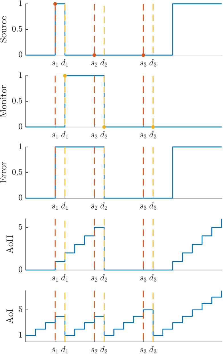
Figure 1: Snapshot of a communication system illustrating the differences between AoI and AoII. In this example, a binary source is sampled at every time slot and is transmitted to the monitor. The packet arrives at the next time slot and is attempted to be decoded. Successful decodings occur at time slots $d_{i}$, $i=1,2,3$, whereas the respective samples were generated at slots $s_{i}=d_{i}-1$. If the decoding is successful, the monitor updates its estimate and the AoI decreases to one (because the sample was generated one time slot ago). Otherwise, the AoI increases. The corresponding error indicates the mismatch between the source and the monitor. The AoII measures the time slots where the error has been positive.

Several works have been published since the introduction of AoII. In [bib:aoii], the authors consider a simple indicator distortion function and study the minimization of AoII under resource constraints, whilst in [bib:aoii_discrete], the distortion function has multiple thresholds. In [bib:aoii_semantics1] and [bib:aoii_semantics2] the results are generalized with task-oriented age functions. In [bib:aoii_pl], the authors analyze the average AoII for a piecewise linear signal where the transmitter updates the monitor for slope changes. The authors in [bib:aoii_multiple_sources2] consider a system with multiple sources where the scheduler is at the side of the receiver. In [bib:aoii_multiple_sources1], a similar problem is studied where the scheduler has imperfect channel state information.

Our work focuses on a discrete-time (slotted) communication system, where each packet has a probability of being successfully decoded. The transmitter and the receiver employ a hybrid automatic repeat request (HARQ) protocol to correct communication errors. In particular, the packets are encoded using a forward error-correction code to correct communication errors at the receiver. If the decoder fails to decode the packet, it requests a re-transmission with a NACK feedback message. When HARQ is used with soft combining, the decoder combines all the received packets to improve the probability of successful decoding [bib:harq_survey, bib:harq_fading]. In the case of soft combining, a re-transmission can either consist of an identical packet (chase combining HARQ) or some complementary information to the previously transmitted packets (incremental redundancy HARQ) [bib:harq_survey]. The standard ARQ protocol is different in that the decoder only detects errors but cannot correct them, and hence discards the previous packets and considers only the most recent ones. This is similar to HARQ without soft combining but without the ability to correct any error. An important aspect of HARQ with soft combining is that the probability of successful decoding increases with the total number of packets while with the simple HARQ and standard ARQ, stays the same.

In this work, we develop optimal scheduling policies for minimizing the average AoII in a communication system with HARQ under a resource constraint. The resource constraint is motivated by limitations on power or network resources (e.g. battery-powered sensors, allocated resources in sensor networks, etc.). The same constraint was considered in [bib:aoii_discrete, bib:aoii_semantics1, bib:aoii, bib:aoii_semantics2] for the minimization of the AoII without HARQ. A related problem is considered in [bib:aoi_harq], where the authors minimize the simple AoI with HARQ under the same constraint. However, the authors give an analytical solution only for the standard ARQ and only approximate the solution for general HARQ protocols. Notably, the analysis of AoII is a harder task than that of the traditional AoI. This stems from the inclusion of the communicated information content in the metric via the distortion function.

To the best of our knowledge, this is the first study that addresses the analysis of the AoII in a communication system with HARQ. The main contributions of this paper are summarized as follows:

• We analyze AoII in a communication scheme utilizing HARQ within the confines of a resource constraint that limits the long-term average transmission rate. We explore HARQ with and without soft combining. The source model employed in this context is an $N$-ary symmetric Markov source.

• The transmission policy optimization problem is framed as a challenging task within the realm of infinite-horizon average-cost constrained Markov decision processes (CMDPs), which are typically known for their difficulty in achieving exact solutions. Nonetheless, an exact solution is attained through an examination of the inherent structural properties of the CMDP.

• Interestingly, we demonstrate that, given certain conditions, the most optimal policy is to abstain from transmission entirely. In all other scenarios, we establish that the optimal approach involves a randomized mixture of two distinct threshold-based policies. We analytically deduce the precise threshold value and the randomization component that align with the resource constraints.

• When considering an HARQ protocol, the state space of the CMDP becomes a union of two countably infinite sets due to tracking the AoII and the transmission count. Handling infinite state spaces poses additional analytical challenges, as documented in [bib:bertsekas, Sec. 4.6]. The primary technical complexity, different from prior research, arises from the interdependence of these variables, making it challenging to establish cost monotonicity. Consequently, the conventional proof of monotonicity employed in threshold-based solutions necessitates a deeper examination of the underlying state transitions within the context of our current work. Additionally, for multivariate-state CMDPs (like in our work), the threshold is an arbitrary function of the other variables, making it generally difficult to find an exact solution. This sets our approach apart from other studies that focus on leveraging the MDP structure to enhance the convergence speed of approximate algorithms rather than seeking an exact solution, as exemplified in references [bib:aoi_harq, 8778671, 8972306, 9085402]. In contrast, we found an analytical solution ready for computation.

• Extensive simulations are conducted to investigate how the average AoII is influenced by the source dynamics, channel conditions, and resource constraints when employing the optimal policy.

The rest of the paper is organized as follows: in Section II, the system model is presented and the problem is formulated as a CMDP. Then, the constrained problem is expressed as an unconstrained Lagrangian MDP. Section III analyzes the structural properties of the Lagrangian MDP and derives the Lagrange-optimal transmission policy. Section LABEL:sec:CMDP shows that the optimal policy of the constrained problem is a randomized mixture of two Lagrange-optimal policies. Section LABEL:sec:Lagrangian_proofs provides the proofs of the structural properties given in Sec. III. Section LABEL:sec:algorithm describes an efficient algorithm that computes the optimal policy, and Section LABEL:sec:results gives numerical results of the average AoII under the optimal policy with varying model parameters. Finally, Section LABEL:sec:conclusion summarizes the main outcomes and presents directions for further extensions.

II Problem Definition

II-A Communication model

We consider a discrete-time (slotted) communication model over a noisy channel. The transmitter monitors a data source from which fresh samples arrive at every time slot. At each time slot, the transmitter decides whether to transmit the fresh sample or discard it. The samples are encoded with a channel coding scheme and sent through the channel to the receiver. Upon receiving the packet, the receiver attempts to decode it. If the decoding is successful, the receiver notifies the transmitter with an ACK packet. Otherwise, it sends a NACK message to ask for additional information. The transmitter decides whether it sends the additional information or rejects the request.

We assume that the channel states of each time slot are independent and identically distributed. Furthermore, we assume that the duration of a packet transmission is constant and equal to one time slot, whilst the ACK/NACK packets are instantaneous. The instantaneous feedback message is a typical assumption in the literature, justified by its limited information content. The constant delay has also been adopted in many other works (e.g. [bib:aoi_harq, bib:aoii, bib:constant_delay_1, bib:constant_delay_2, bib:constant_delay_3, bib:constant_delay_4]). Note that in typical networks there are two major sources of randomness in the delay: a) queues formed by packet congestion in relay nodes and b) erroneous packets that need to be re-transmitted. In our work, we abstract the stochasticity of the delay due to erroneous packets and embed it in a model with a constant delay and a specified probability of successful decoding. Therefore, our model is close to reality when the randomness incurred by queues is negligible.

The probability of successful decoding at each time slot is specified by a non-decreasing function $p(r)\in(0,1)$, where $r\in\mathbbm{N}$ is the number of packets already gotten by the receiver. For example, the probability of successful decoding for the first packet is given by $p(0)$, for the second packet is given by $p(1)$, and so on. Typically, the maximum number of packets is limited and only a total of $r_{max}$ re-transmissions are allowed [bib:harq_survey].

Our objective is to minimize the average AoII. In particular, let $g(X_{t},\hat{X_{t}})$ denote the distortion function at time $t$ between the source $X_{t}$ and its estimation $\hat{X_{t}}$ at the receiver. In general, $g(X_{t},\hat{X_{t}})$ is directed by the specific application of interest. Moreover, the age function is defined as

$$\Delta_{t}\triangleq t-h_{t}\,,$$ (1)

where $h_{t}$ is the last time instant when the distortion $g(X_{t},\hat{X_{t}})$ was zero. The instantaneous AoII at time $t$ is simply the product of the age and distortion functions,

$$\delta_{t}\triangleq\Delta_{t}\cdot g(X_{t},\hat{X_{t}}).$$ (2)

We shall generalize the AoII process in (2) by employing a generic monotonically increasing and unbounded penalty function $f(\delta_{t})$, i.e., $f(\delta^{\prime})>f(\delta)\ \forall\ \delta^{\prime}>\delta$ and $\lim_{\delta\to+\infty}f(\delta)=+\infty$.

Lastly, motivated by requirements on saving or allocating power and network resources, we impose a constraint on the transmission rate by requiring the long-term transmission rate to not exceed $R\in(0,1]$.

II-B Source Model

Hereafter, we focus on $N$-ary symmetric Markov sources, as illustrated in Fig. 2. Here, $\alpha$ is the probability that the source remains at the same state at the next time slot, and $\mu$ is the probability of transition to all other $N-1$ states. The same model is considered in [bib:aoii] and [bib:aoii_multiple_sources2].

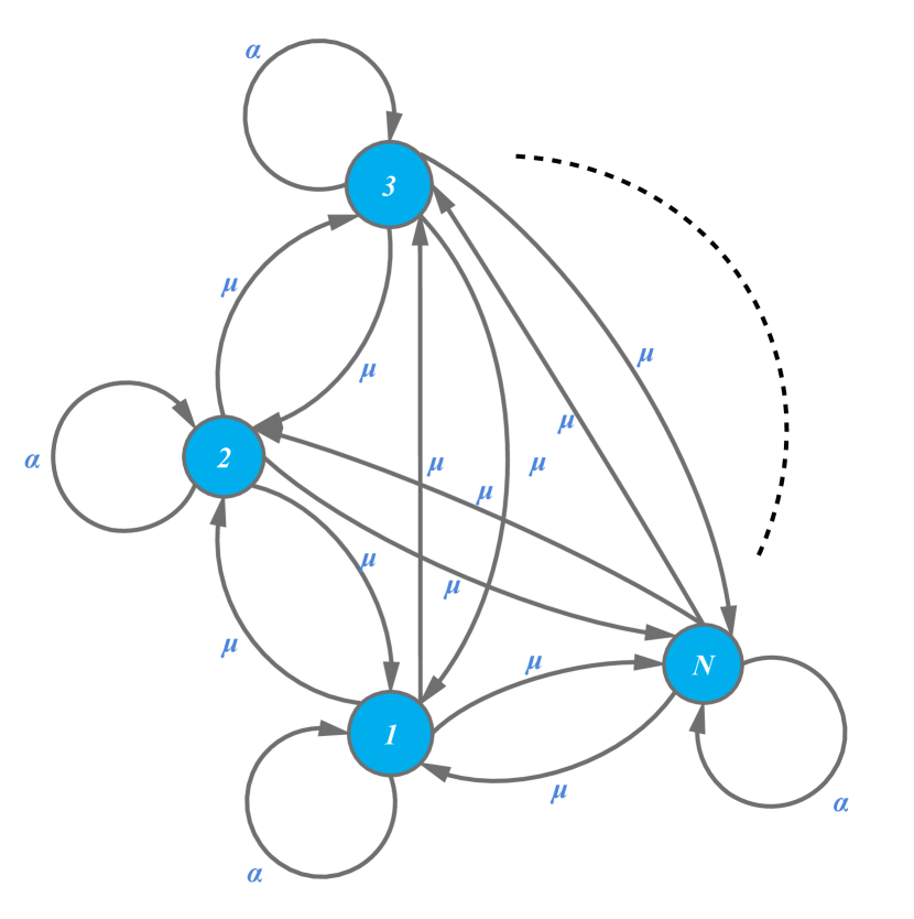
Figure 2: The symmetric Markov data source under consideration.

Due to the normalization property of the transition probabilities, the following equality must hold,

$$(N-1)\mu+\alpha=1.$$ (3)

In our analysis, we employ an indicator distortion function defined as follows,

$$g(X_{t},\hat{X_{t}})=\mathbbm{1}_{\{X_{t}\neq\hat{X_{t}}\}}\,.$$ (4)

This distortion function penalizes equally any information mismatch between the source and the monitor. The symmetric Markov source implies that the source changes (or gives new information) every $Y$ time slots, where $Y$ is geometrically distributed, with the same parameter for all states. Note that the indicator cost function may also arise by truncating other more complex distortion functions, i.e., it can model the function $\mathbbm{1}_{\{d(X_{t},\hat{X_{t}})>c\}}\,$, where $d(X_{t},\hat{X_{t}})$ is any distortion function and $c$ is a specified threshold. In this case, we lose some information but gain the tractability of the optimization problem.

Although we focus on finite-state Markov chains, our results also hold for infinite-state Markov chains. This adds to the versatility of our results. We note two interesting cases in this matter. Firstly, suppose that $\alpha\!=\!0$ and $N\!\rightarrow\!\infty$. Thus, the source gives new information at every time slot, but the information at two different time slots is never the same. This implies that the AoII falls back to the simple AoI. Secondly, suppose that the real source is a finite-state Markov chain with a fixed probability of staying at the same state $\alpha\!>\!0$. Now construct another Markov chain that is infinite-state but with the same probability of staying at the same state $\alpha$. We have $\alpha\!>\!0,\ N\!\rightarrow\!\infty,\ \mu\!\rightarrow\!0$. With the constructed Markov chain, once the source departs from a state, the probability of returning to it in the future is zero. This reflects the scenario where the AoII penalty is zero if there is no new information but always increases otherwise, even if the real source eventually returns to the known value. This model can be used when the generation time of the information is part of the information itself.

II-C Mathematical Formulation

We formulate the problem as an infinite-horizon average-cost constrained Markov decision process (CMDP). The next subsections define the CMDP and present the necessary assumptions.

II-C1 Definition of the Constrained Markov Decision Process

Before we define the CMDP, we highlight a remark that simplifies the definition of the problem. In particular, the transmitter is not obliged to fulfil the request for a re-transmission. However, should a re-transmission occur, it is better to do it immediately after receiving the NACK message than wait some time. This is true since waiting i) increases the age and ii) incurs the chance of the packet becoming obsolete due to a change of the source, all without increasing the probability of decoding. A similar observation has been made in the study of AoI with HARQ [bib:aoi_harq].

Remark 1.

The AoII-optimal transmission policy incurs an HARQ re-transmission only immediately after the reception of a NACK feedback message.

Therefore, we presume that if the transmitter decides to not fulfil the re-transmission request immediately, the request is rejected altogether and the transmission count $r$ reverts to zero.

That being so, the CMDP is defined as follows:

• The state of the CMDP at time $t$ is given by $S_{t}=(\delta_{t},r_{t})\in\mathcal{S}$, where $\delta_{t}$ is the AoII at the current time slot and $r_{t}$ is the transmission count for the current source state.

• The cost at state $S_{t}$ is equal to the instantaneous AoII penalty $f(\delta_{t})$.

• The actions $y_{t}\in\mathcal{Y}$, where the action space $\mathcal{Y}=\{0,1\}$ consists of the “wait” ($y_{t}=0$) and the “transmit” ($y_{t}=1$) actions.

• Define the functions $\gamma_{1}(r_{t})$, $\gamma_{2}(r_{t})$ as

  $$\gamma_{1}(r_{t})\triangleq\alpha(1-p(r_{t})),$$ (5)

  $$\gamma_{2}(r_{t})\triangleq 1-\alpha-\mu(1-p(r_{t})).$$ (6)

  The transition probabilities are summarized as follows, while a detailed derivation is given in the Appendix.  
  

  If action is “wait” ($y_{t}=0$):

  $$P(S_{t+1}{=}(\delta_{t}{+}1,0)\mid\delta_{t}>0,r_{t}\geq 0,y_{t}=0)=1-\mu\,,$$ (7)

  $$P(S_{t+1}{=}(0,0)\mid\delta_{t}>0,r_{t}\geq 0,y_{t}=0)=\mu\,,$$

  $$P(S_{t+1}{=}(1,0)\mid\delta_{t}=0,r_{t}=0,y_{t}=0)=1-\alpha\,,$$

  $$P(S_{t+1}{=}(0,0)\mid\delta_{t}=0,r_{t}=0,y_{t}=0)=\alpha\,.$$

  If action is “transmit” ($y_{t}=1$):

  $$P(S_{t+1}{=}(\delta_{t}{+}1,r_{t}{+}1)\mid\delta_{t}>0,r_{t}\geq 0,y_{t}=1)=\gamma_{1}(r_{t})\,,$$ (8)

  $$P(S_{t+1}{=}(\delta_{t}{+}1,0)\mid\delta_{t}>0,r_{t}\geq 0,y_{t}=1)=\gamma_{2}(r_{t})\,,$$

  $$P(S_{t+1}{=}(0,0)\mid\delta_{t}\!>\!0,r_{t}\!\geq\!0,y_{t}\!=\!1)=1\!-\!\gamma_{1}(r_{t})\!-\!\gamma_{2}(r_{t})\,,$$

  $$P(S_{t+1}{=}(1,0)\mid\delta_{t}=0,r_{t}=0,y_{t}=1)=1-\alpha\,,$$

  $$P(S_{t+1}{=}(0,0)\mid\delta_{t}=0,r_{t}=0,y_{t}=1)=\alpha\,.$$

• The long-term average number of “transmit” actions is constrained to not exceed $R\in(0,1]$.

II-C2 Additional Assumptions

To derive our results, it is necessary to impose the following condition, which ensures that the average AoII is finite under the policy that a new transmission is performed in every time slot,

$$\sum_{l=1}^{\infty}f(l{+}1)(\gamma_{1}(0)+\gamma_{2}(0))^{l}<\infty\,.$$ (9)

Furthermore, without loss of generality, we assume an unlimited maximum number of allowed re-transmissions, i.e., $r_{max}=\infty$. In Section LABEL:sec:results, we impose a finite $r_{max}$ without affecting the theoretical results.

II-C3 Definition of the Optimization Problem

The optimization problem pertains to finding the policy $\pi:\mathcal{S}\mapsto\mathcal{Y}$ that minimizes the long-term average AoII, while not exceeding the transmission rate constraint. The problem can be expressed as a linear programming problem, as follows,

Definition 1 (Main CMDP Problem).

Minimize $$J_{\pi}(S_{0})\!\triangleq\!\limsup\limits_{T\rightarrow\infty}\frac{1}{T}E_{\pi}\!\left[\sum_{t=0}^{T-1}f(\delta_{t})\mid S_{0}\right]$$ (10)

subject to $$C_{\pi}(S_{0})\!\triangleq\!\limsup\limits_{T\rightarrow\infty}\frac{1}{T}E_{\pi}\!\left[\sum_{t=0}^{T-1}y_{t}\mid S_{0}\right]\!\leq\!R\,.$$

To solve the constrained problem, we introduce the Lagrangian average cost and solve the relaxed problem,

Definition 2 (Lagrangian MDP Problem).

$$\text{Minimize}\;J(\pi{,}\lambda){\triangleq}{\lim\limits_{T\rightarrow\infty}}\!\sup\limits_{\lambda\geq 0}\!\frac{1}{T}E_{\pi}{\left[\sum_{t=0}^{T-1}f(\delta_{t}){+}\lambda y_{t}\mid S_{0}\right]}{-}\lambda R\,.$$ (11)

For any fixed value of $\lambda$, let

$$\pi_{\lambda}\triangleq\operatorname*{\arg\!\min}_{\pi}J(\pi,\lambda)\,,$$ (12)

$$g\triangleq\min_{\pi}J(\pi,\lambda)\,,$$ (13)

denote the optimal policy of the Lagrangian MDP and the average cost achieved by the optimal policy, respectively.

The following lemma provides the means for an alternative mathematical formulation.

Lemma 1.

The MDP (11) is unichain. That is, there exists a single recurrent class and a (possibly empty) transient class.

Proof.

From the transition probabilities (7), (8), we observe that, under any policy, there is a positive probability from every state to transit to state $S=(0,0)$. This suffices to prove the statement.∎

Due to Lemma 1 and [bib:krishnamurthy, Thm. 6.5.2], the optimal policy $\pi_{\lambda}$ can be found by solving the following Bellman equations,

$$g+V(S_{t})=\min_{y_{t}}\{f(\delta_{t})+\lambda y_{t}+\sum_{S_{t+1}}P(S_{t+1}\!\mid\!S_{t},y_{t})V(S_{t+1})\}.$$ (14)

The function $V(S_{t})=V(\delta_{t},r_{t})$ is called the value function of state $S_{t}$.

In the following, Section III elaborates on the Lagrangian MDP, and Section LABEL:sec:CMDP reverts to the main CMDP to define the optimal policy. The proofs of the results of Sec. III are written in Sec. LABEL:sec:Lagrangian_proofs, while the results of Sec. LABEL:sec:CMDP are given in the Appendix.

III Structural Results For The Lagrangian Problem

This section gives the structural properties of the Lagrangian MDP. All results given here are proved in Section LABEL:sec:Lagrangian_proofs.

The following two lemmas characterize how varying $\delta$ or $r$ affects the value function $V(\delta,r)$ and are necessary for proving the structural property of the optimal transmission policy.

Lemma 2.

The function $V(\delta,r)$ is increasing w.r.t. $\delta$.

Lemma 3.

If $\mu<\alpha$, the function $V(\delta,r)$ is non-increasing w.r.t. $r$. If $\mu\geq\alpha$, it is non-decreasing.

Our first main result is given by the following proposition:

Proposition 1.

Given a fixed transmission count $r$, if $\mu<\alpha$, the optimal policy at state $S=(\delta,r)$ is threshold-based w.r.t. $\delta$. If $\mu\geq\alpha$, the optimal policy is to always wait.

Proposition 1 reveals that when the probability $\alpha$ is too small, communication is inadequate in reducing the AoII. This is a natural consequence since a transmission is useful only when the most likely state at the time of reception is the one being transmitted. Notice that a more sophisticated estimator at the receiver would leverage the received state to estimate a different state as the most probable. However, this would require the knowledge of the source dynamics at the side of the receiver, which is a rather strict assumption.

As a corollary of Proposition 1, the average AoII for $\mu\geq\alpha$ can be found by solving for $g$ in (14), which is easy to do since the optimal policy is $y=0$ for all steps.

Corollary 1.

If $\mu\geq\alpha$, the average AoII under the optimal (waiting) policy is given by

$$g_{wait}=\frac{\mu\left(f(0)+(1-\alpha)\sum_{i=1}^{\infty}(1-\mu)^{i}f(i)\right)}{(1-\alpha)(1-\mu)+\mu}\,.$$ (15)

On the other hand, for $\mu<\alpha$, Proposition 1 states that for a fixed $r$ there exist a corresponding threshold $n^{*}_{r,\lambda}$, such that for all states $S=(\delta,r)$ with $\delta\geq n^{*}_{r,\lambda}\,$ the optimal policy is $y=1$, whereas if $\delta<n^{*}_{r,\lambda}$ the optimal policy is $y=0$. The next proposition implies that it suffices to define only the threshold for $r=0$, $n^{*}_{0,\lambda}$.

Proposition 2.

Let $n^{*}_{r,\lambda}$ denote the optimal threshold when the transmission count equals $r$. The sequence $\{n^{*}_{r,\lambda}\}$ is non-increasing w.r.t. $r$.

We elaborate on the consequences of Proposition 2. Suppose that the system has reached the state $S_{t}=(\delta_{t},r_{t})$, $\delta_{t}\!>\!0$, $r_{t}\!>\!0$. Since $r_{t}$ is positive, it follows that the previous state was $S_{t-1}=(\delta_{t}{-}1,r_{t}{-}1)$ and the optimal action was $y_{t-1}=1$. Therefore, it holds that $\delta_{t}\!-\!1\!\geq\!n^{*}_{r_{t}-1,\lambda}\,$, which implies that $\delta_{t}\!>\!n^{*}_{r_{t},\lambda}$ due to Proposition 2. It follows that the optimal action for the state $S_{t}$ is also $y_{t}\!=\!1$. By induction, we infer that it suffices to find the threshold $n^{*}_{0,\lambda}$. After the instantaneous AoII reaches $n^{*}_{0,\lambda}$, the optimal action is to always transmit until the AoII becomes zero.

Exploiting the previous results, we can derive the following Theorem, which describes the solution to the Lagrangian MDP problem (11).

Theorem 1.

The optimal threshold $n^{*}_{0,\lambda}$ is equal to

$$n^{*}_{0,\lambda}=\min\{ n_{0}\in\mathbbm{N^{*}}:$$ (16)

$$(1\!-\!\mu)V(n_{0}{+}1,0)\!-\!V(n_{0},0)\!+\!f(n_{0})\!-\!g_{n_{0}}\!>\!0\},$$

where $g_{n_{0}}$ is the average cost achieved by the threshold $n_{0}$. The values of $V(n_{0},0)$, $V(n_{0}{+}1,0)$ and $g_{n_{0}}$ are computed via the expressions in Table LABEL:tab:opt_policy_analytic.

 

$$V(\delta,0)=\sum_{l=0}^{\infty}\left[\left(f(\delta{+}l)+\lambda-g_{n_{0}}\right)\sum_{i=0}^{\infty}P_{0,i}^{l}\right],\quad\text{for $\delta\geq n_{0}$}\,.$$

$$g_{n_{0}}=\frac{\frac{f(0)}{1-\alpha}+\sum\limits_{i=0}^{n_{0}-2}(1-\mu)^{i}f(i{+}1)+(1-\mu)^{n_{0}-1}\sum\limits_{l=0}^{\infty}\left[\left(f(n_{0}{+}l)+\lambda\right)\sum\limits_{i=0}^{\infty}P_{0,i}^{l}\right]}{\frac{1}{1-\alpha}+\sum\limits_{i=0}^{n_{0}-2}(1-\mu)^{i}+(1-\mu)^{n_{0}-1}\sum\limits_{l=0}^{\infty}\sum\limits_{i=0}^{\infty}P_{0,i}^{l}},$$

where

$$P\triangleq \begin{array}{cccccccc}& 0& 1& 2& 3& 4& \mathrm{\dots }& j\\ 0& \gamma {}_2(0)& \gamma {}_1(0)& 0& 0& 0& \mathrm{\dots }& 0\\ 1& \gamma {}_2(1)& 0& \gamma {}_1(1)& 0& 0& \mathrm{\dots }& 0\\ 2& \gamma {}_2(2)& 0& 0& \gamma {}_1(2)& 0& \mathrm{\dots }& 0\\ \mathrm{⋮}& \mathrm{⋮}& & & & \mathrm{\ddots }& & \mathrm{⋮}\\ \mathrm{⋮}& \mathrm{⋮}& & & & & \mathrm{\ddots }& \mathrm{⋮}\\ j-1& \gamma {}_2(j-1)& 0& 0& 0& 0& \mathrm{\dots }& \gamma {}_1(j-1)\\ j& \gamma {}_2(j)& 0& 0& 0& 0& \mathrm{\dots }& 0\end{array}$$