Status Updating under Partial Battery Knowledge in Energy Harvesting IoT Networks

Abstract

We study status updating under inexact knowledge about the battery levels of the energy harvesting sensors in an IoT network, where users make on-demand requests to a cache-enabled edge node to send updates about various random processes monitored by the sensors. To serve the request(s), the edge node either commands the corresponding sensor to send an update or uses the aged data from the cache. We find a control policy that minimizes the average on-demand AoI subject to per-slot energy harvesting constraints under partial battery knowledge at the edge node. Namely, the edge node is informed about sensors’ battery levels only via received status updates, leading to uncertainty about the battery levels for the decision-making. We model the problem as a POMDP which is then reformulated as an equivalent belief-MDP. The belief-MDP in its original form is difficult to solve due to the infinite belief space. However, by exploiting a specific pattern in the evolution of beliefs, we truncate the belief space and develop a dynamic programming algorithm to obtain an optimal policy. Moreover, we address a multi-sensor setup under a transmission limitation for which we develop an asymptotically optimal algorithm. Simulation results assess the performance of the proposed methods.

I Introduction

In future Internet of things (IoT) systems, timely delivery of status updates about a remotely monitored random process to a destination is the key enabler for the emerging time-critical applications, e.g., drone control, smart home, and transport systems. Such destination-centric information freshness can be quantified by the age of information (AoI) [1, 2]. On the other hand, IoT networks with low-power sensors are subject to stringent energy limitations, which is often counteracted by energy harvesting (EH) technology. To summarize, these emerging applications require designing AoI-aware status updating control that both guarantees timely status delivery and accounts for the limited energy resources of EH sensors.

In this paper, we consider a status update IoT network consisting of EH sensors, users, and an edge node, which acts as a gateway between the sensors and users, as depicted in Fig. 1. The users are interested in time-sensitive information about several random processes, each measured by a sensor. The users send requests to the edge node that has a cache storage to store the most recently received status update from each sensor. To serve a user’s request, the edge node either commands the corresponding sensor to send a fresh status update or uses the aged data from the cache. This introduces an inherent trade-off between the age of information (AoI) at the users and the energy consumption of the sensors. As the main novelty of our work compared to the related AoI-aware network designs [3, 4, 5, 6], we consider a practical scenario where the edge node is informed of the sensors’ battery levels only via the received status updates, leading to partial battery knowledge at the edge node. Particularly, our objective is to find the best actions of the edge node to minimize the average AoI of the served measurements, i.e., average on-demand AoI. Accounting for the partial battery knowledge, we model this as an average-cost partially observable Markov decision process (POMDP). We then convert the POMDP into a belief-state MDP and, via characterizing its key structures, develop an iterative algorithm to obtain an optimal policy. Further, we extend the proposed approach to the multi-sensor setup under a transmission constraint, where only a limited number of sensors can send status updates at each time slot. Numerical experiments assess the performance of the proposed methods.

I-A Contributions

The primary contributions of our study are summarized as follows:

• We consider (on-demand) AoI-minimization for a status update IoT network where the decision-maker does not know the exact battery levels of the sensors at each slot. Accounting for the partial battery knowledge, we model the problem as an average-cost POMDP.

• We reformulate the POMDP into an equivalent belief-MDP which, however, is difficult to solve in its original form due to the infinite belief space. Fortunately, we exploit a certain pattern in the evolution of beliefs to truncate the belief space and develop a dynamic programming algorithm that obtains an optimal policy. In addition, we derive an efficient algorithm implementation by exploiting the inherent sparsity of the transition matrices.

• Further, we extend the proposed approach to the multi-sensor setup under a transmission constraint, where only a limited number of sensors can send status updates at each time slot. In particular, we develop a low-complexity relax-then-truncate algorithm and show its asymptotic optimality as the number of sensors approaches infinity.

• Numerical experiments illustrate the threshold-based structure of an optimal policy and show the gains obtained by the proposed optimal POMDP-based policy compared to a request-aware greedy policy. Further, numerical experiments depict that the proposed relax-then-truncate method has near-optimal performance even for moderate numbers of sensors in multi-sensor scenarios under a transmission constraint.

To the best of our knowledge, this is the first work that derives an optimal policy for AoI minimization in a network with EH sensors, where the decision-making relies only on partial battery knowledge about the sensors’ battery levels.

I-B Related Works

AoI-aware scheduling has witnessed a great research interest the last few years. The works [7, 8, 9, 10, 11, 12, 13, 14, 15, 16, 17, 18, 19, 20] consider a sufficient power source whereby an update can be sent any time. Differently, [21, 22, 23, 24, 25, 26, 27, 28, 3, 29, 30] consider that the source nodes are powered by energy harvested from the environment; thus, AoI-aware scheduling is carried out under the energy causality constraint at the source nodes. Also, while the above works (implicitly) assume that time-sensitive information is needed at the destination at all time moments, [4, 5, 31, 6, 32, 33, 34] study information freshness of the source(s) driven by users’ requests. Particularly, in our prior research [4, 3, 5, 6], we introduced the concept of on-demand AoI. This metric quantifies the freshness of information seen by users in request-based status updating systems. In [4, 3, 5, 6], we have mainly focused on optimal scheduling under the assumption that the decision-maker (i.e., the edge node) possessed precise knowledge of the sensors’ battery levels at every time slot. However, such an assumption necessitates continuous coordination between the sensors and the edge node, which may not always be feasible in practical scenarios. In contrast, this study delves into optimal scheduling under partial battery knowledge at the edge node, a scenario that can be effectively modeled as a POMDP.

A few works have applied POMDP formulation, in which the state of the system is not fully observable to the decision maker, in AoI-aware design [15, 16, 17, 18, 25]. In [15], the authors proposed POMDP-based AoI-optimal transmission scheduling in a status update system under an average energy constraint and uncertain channel state information. In [16], the authors proposed an age-aware scheduling policy for a multi-user uplink system under partial knowledge of the status update arrivals at the monitor node. In [17], the authors investigated AoI-optimal scheduling in a wireless sensor network where the AoI values of the sensors are not directly observable by the access point. In [18], the authors derived an optimal sensor probing policy in an IoT network with intermittent faults and inexact knowledge about the status (healthy or faulty) of the system. In [19], the authors derived age-aware POMDP-based scheduling for a wireless multi-user uplink network with partial observations of the local ages at end devices. In [25], the authors investigated AoI minimization for an EH cognitive secondary user with either perfect or imperfect spectrum sensing. Preliminary results of this paper appear in [32].

I-C Organization

The structure of the paper is outlined as follows. For the sake of clarity in presentation, we first restrict ourselves to the single-sensor scenario, and then, we address the multi-sensor scenario under the transmission constraint. In particular, Section II describes the single-sensor system setup and the problem formulation. In Section III, we propose a novel POMDP-based approach that finds an optimal policy for the single-sensor setup. In Section IV, we address the multi-sensor scenario under a transmission constraint. In Section V, we evaluate the performance of the proposed methods through simulations. Finally, in Section VI, we conclude the paper.

II Single-Sensor System Model and Problem Formulation

Figure 1: An IoT sensing network with $K$ EH sensors, an edge node, and users, which are interested in timely status update information of the physical processes monitored by the sensors.

II-A Network Model

We consider a status update system, where an energy harvesting (EH) sensor (e.g., sensor 1 in Fig. 1) sends status updates about the monitored random process to users via a cache-enabled edge node, which acts as a gateway between the sensors and the users. A time-slotted system with slots ${t\in\mathbb{N}}$ is considered. We consider request-based status updating, where, at the beginning of slot $t$, users request for the status of the sensor (i.e., a new measurement) from the edge node. The edge node, which has a cache that stores the most recently received status update from the sensor, handles the arriving requests during the same slot $t$. Let ${r(t)\in\{0,1\}}$, ${t=1,2,\dots}$, denote the random process of requesting the status of the sensor at slot $t$; ${r(t)=1}$ if the status is requested (by at least one user) and ${r(t)=0}$ otherwise. The requests are independent across time slots and the probability of having a request at each time slot is ${p=\mathrm{Pr}\{r(t)=1\}}$. Upon receiving a request at slot $t$, the edge node serves the requesting user(s) by either 1) commanding the sensor to send a fresh status update packet or 2) using the stored measurement from the cache. Let ${a(t)\in\mathcal{A}=\{0,1\}}$ be the command action of the edge node at slot $t$; ${a(t)=1}$ if the edge node commands the sensor to send an update and ${a(t)=0}$ otherwise.

II-B Energy Harvesting Sensor

The sensor operates by harvesting energy from the environment and storing it into a battery of finite capacity $B$ (units of energy). We model the energy arrivals ${e(t)\in\left\{0,1\right\}}$, ${t=1,2,\dots}$, as a Bernoulli process with rate ${\lambda=\Pr\{e(t)=1\}}$, $\forall t$. This characterizes the discrete nature of the energy arrivals in a slotted-time system, i.e., at each time slot, a sensor either harvests one unit of energy or not (see e.g., [4, 6, 22, 35]). We denote the battery level of the sensor at the beginning of slot $t$ by ${b(t)\in\{0,\ldots,B\}}$. We assume that measuring and transmitting a status update from the sensor to the edge node consumes one unit of energy (see, e.g., [4, 6, 15, 22, 21]). Thus, if the sensor is commanded to send an update (i.e., $a(t)=1$), it can only do so if its battery is not empty (i.e., $b(t)\geq 1$). Let $d(t)\in\{0,1\}$ indicate the sensor’s action at slot $t$; $d(t)=1$ if a status update is sent, and $d(t)=0$ otherwise. Thus, ${d(t)=a(t)\mathds{1}_{\{b(t)\geq 1\}}}$, where ${\mathds{1}_{\{\cdot\}}}$ is the indicator function. Finally, the evolution of the battery level is given by

$$b(t+1)=\min\left\{b(t)+e(t)-d(t),B\right\}.$$ (1)

II-C Status Updating with Partial Battery Knowledge

As the main distinctive feature of this paper, we consider a practical operation mode of the network in which the edge node is informed about the sensor’s battery level (only) via the received status update packets. Specifically, each status update packet contains the measured value (status) of the physical quantity, a time stamp representing the time when the sample was generated, and the current battery level of the sensor. As the inevitable consequence of this status updating procedure, the edge node has only partial knowledge about the battery level at each slot, i.e., outdated knowledge based on the sensor’s last update. It is worth emphasizing that considering this realistic setting is in stark contrast to the previous works on AoI-aware network designs (see e.g., [5, 31, 6, 27]) which all assume that perfect battery knowledge is available at the decision-maker (herein, the edge node) at each slot.

Formally, let ${\tilde{b}(t)\in\{1,2,\dots,B\}}$ denote the edge node’s knowledge about the sensor’s battery level at slot $t$. At slot $t$, let $u(t)$ denote the most recent slot in which the edge node received a status update packet, i.e., ${u(t)=\max\{t^{\prime}|t^{\prime}<t,d(t^{\prime})=1\}}$. Thus, the true battery level and the knowledge about the level are interrelated as ${\tilde{b}(t)=b(u(t))}$. Specifically, at slot $t$, $\tilde{b}(t)$ indicates what the sensor’s battery level was at the beginning of the most recent slot at which the edge node received a status update. Henceforth, we refer to $\tilde{b}(t)$ as the partial battery knowledge.

II-D On-Demand Age of Information

We use the on-demand AoI metric [4, 5] to measure the freshness of information seen by the users in our request-based status updating system. Let $\Delta(t)$ be the AoI about the monitored process at the edge node at the beginning of slot $t$, i.e., the number of slots elapsed since the generation of the latest received update, which is expressed as ${\Delta(t)=t-u(t)}$. We make a common assumption (see e.g., [17, 33, 28, 27, 26, 25, 24, 23, 11, 7]) that $\Delta(t)$ is upper-bounded by a sufficiently large value $\Delta^{\mathrm{max}}$, i.e., ${\Delta(t)\in\{1,2,\ldots,\Delta^{\mathrm{max}}\}}$. In addition to tractability, this makes further counting unnecessary once the available measurement becomes excessively outdated. The evolution of $\Delta(t)$ is given by

$$\Delta(t+1)=\left\{\begin{array}[]{ll}1,&\mathrm{if}\leavevmode\nobreak\ d(t)=1,\\ \min\{\Delta(t)+1,\Delta^{\mathrm{max}}\},&\mathrm{if}\leavevmode\nobreak\ d(t)=0,\end{array}\right.$$ (2)

which can be written in a compact form as $\Delta(t+1)=\min\{(1-d(t))\Delta(t)+1,\Delta^{\mathrm{max}}\}$.

We define on-demand AoI at slot $t$ as

$$\Delta^{\mathrm{OD}}(t)\triangleq r(t)\Delta(t+1)=r(t)\min\{(1-d(t))\Delta(t)+1,\Delta^{\mathrm{max}}\}.$$ (3)

Referring to (3), the requests are made at the beginning of slot $t$ and measurements are sent by the edge node at the end of the same slot, thus, $\Delta(t+1)$ is the AoI perceived by the users.

II-E Problem Formulation

We aim to find the best action of the edge node at each time slot, i.e., $a(t)$, $t=1,2,\ldots$, called an optimal policy, that minimizes the average cost (i.e., average on-demand AoI), defined as

$$\bar{C}=\lim_{T\rightarrow\infty}\frac{1}{T}\sum_{t=1}^{T}\mathbb{E}[\Delta^{\mathrm{OD}}(t)],$$ (4)

where the expectation is taken over all system dynamics, i.e., random process of energy arrivals and requests, as well as the (possibly randomized) policy constructed in response to the requests.

III POMDP Modeling, Optimal Policy, and Proposed Algorithm

We model the problem of finding an optimal policy as a partially observable Markov decision process (POMDP) and develop an iterative algorithm to find such an optimal policy.

III-A POMDP Modeling

The POMDP is defined by a tuple $(\mathcal{S},\mathcal{O},\mathcal{A},\Pr(s(t+1)|s(t),a(t)),\Pr(o(t)|s(t),a(t-1)),c(s(t),a(t)))$ [36, Chap. 7], with the following elements.

• State Space $\mathcal{S}$: Let ${s(t)\in\mathcal{S}}$ denote the system state at slot $t$, which we define as ${s(t)=(b(t),r(t),\Delta(t),\tilde{b}(t))}$, where ${b(t)\in\{0,1,\ldots,B\}}$ is the battery level, ${r(t)\in\{0,1\}}$ is the request indicator, ${\Delta(t)\in\{1,2,\ldots,\Delta^{\mathrm{max}}\}}$ is the AoI, and ${\tilde{b}(t)\in\{1,2,\dots,B\}}$ is the partial battery knowledge. The state space $\mathcal{S}$ has a finite dimension ${|\mathcal{S}|=2B(B+1)\Delta^{\mathrm{max}}}$. We denote the observable part of the state (i.e., visible by the edge node) by ${s^{\mathrm{v}}(t)=(r(t),\Delta(t),\tilde{b}(t))}$; thus, ${s(t)=(b(t),s^{\mathrm{v}}(t))}$.

• Observation Space $\mathcal{O}$: Let ${o(t)\in\mathcal{O}}$ be the edge node’s observation about the system state at slot $t$. We define it as the visible part of the state, i.e., ${o(t)=s^{\mathrm{v}}(t)}$. The observation space $\mathcal{O}$ has a finite dimension $|\mathcal{O}|=2B\Delta^{\mathrm{max}}$.

• Action Space $\mathcal{A}$: At each slot, the edge node decides whether to command the sensor or not, i.e., ${a(t)\in\mathcal{A}=\{0,1\}}$.

• State Transition Probability $\Pr(s(t+1)|s(t),a(t))$: The state transition probability specifies the probability of transitioning from current state ($s(t)$) ${s=(b,r,\Delta,\tilde{b})}$ to next state ($s(t+1)$) ${s^{\prime}=(b^{\prime},r^{\prime},\Delta^{\prime},\tilde{b}^{\prime})}$ when taking a particular action ${a(t)=a}$, which is given by

  $$\begin{array}[]{ll}\Pr(b^{\prime},r^{\prime},\Delta^{\prime},\tilde{b}^{\prime}\mid b,r,\Delta,\tilde{b},a)=\Pr\big{(}r^{\prime}\big{)}\Pr(b^{\prime},\mid b,a)\Pr(\Delta^{\prime},\tilde{b}^{\prime}\mid b,\tilde{b},\Delta,a),\end{array}$$ (5)

  where

  $${\Pr(r^{\prime})=pr^{\prime}+(1-p)(1-r^{\prime}),\leavevmode\nobreak\ \leavevmode\nobreak\ \leavevmode\nobreak\ r^{\prime}\in\{0,1\}}$$ (6)

  $$\Pr(b^{\prime}\mid b=B,a=0)=\mathds{1}_{\{b^{\prime}=B\}},\leavevmode\nobreak\ b^{\prime}\in\{0,1,\dots,B\},$$ (7)

  $$\Pr(b^{\prime}\mid b<B,a=0)=\left\{\begin{array}[]{ll}{\lambda,}&b^{\prime}=b+1,\\ {1-\lambda,}&b^{\prime}=b,\\ 0,&\mbox{otherwise.}\end{array}\right.$$

  $$\Pr(b^{\prime}\mid b=0,a=1)=\left\{\begin{array}[]{ll}{\lambda,}&b^{\prime}=1,\\ {1-\lambda,}&b^{\prime}=0,\\ 0,&\mbox{otherwise.}\end{array}\right.$$

  $$\Pr(b^{\prime}\mid b\geq 1,a=1)=\left\{\begin{array}[]{ll}{\lambda,}&b^{\prime}=b,\\ {1-\lambda,}&b^{\prime}=b-1,\\ 0,&\mbox{otherwise.}\end{array}\right.$$

  $$\Pr(\Delta^{\prime},\tilde{b}^{\prime}\mid b,\tilde{b},\Delta,a=0)=\mathds{1}_{\{\Delta^{\prime}=\min\{\Delta+1,\Delta^{\mathrm{max}}\},\tilde{b}^{\prime}=\tilde{b}\}},$$ (8)

  $$\Pr(\Delta^{\prime},\tilde{b}^{\prime}\mid b=0,\tilde{b},\Delta,a=1)=\mathds{1}_{\{\Delta^{\prime}=\min\{\Delta+1,\Delta^{\mathrm{max}}\},\tilde{b}^{\prime}=\tilde{b}\}},$$

  $$\Pr(\Delta^{\prime},\tilde{b}^{\prime}\mid b\geq 1,\tilde{b},\Delta,a=1)=\mathds{1}_{\{\Delta^{\prime}=1,\tilde{b}^{\prime}=b\}}.$$

• Observation Function ${\Pr(o(t)\mid s(t),a(t-1))}$: The observation function is the probability of observing $o(t)$ given a state $s(t)$ and an action $a(t-1)$. In our model, this is given by ${\Pr(o(t)|s(t),a(t-1))=\Pr({o(t)}|b(t),s^{\mathrm{v}}(t),a(t-1))=\mathds{1}_{\{o(t)=s^{\mathrm{v}}(t)\}}}$.

• Immediate Cost Function $c(s(t),a(t))$: The immediate cost of taking action $a(t)$ in state ${s(t)=(b(t),r(t),\Delta(t),\tilde{b}(t))}$ is ${c(s(t),a(t))=r(t)\min\{(1-a(t)\mathds{1}_{\{b(t)\geq 1\}})\Delta(t)+1,\Delta^{\mathrm{max}}\}}$.

III-B Belief-State

As the POMDP formulation above implies, the system state $s(t)$ is not fully observable by the edge node – the decision-maker – at slot $t$. To reiterate, the state consists of two parts as ${s(t)=(b(t),s^{\mathrm{v}}(t))}$. Consequently, at slot $t$, the exact battery level $b(t)$ is unknown to the edge node, whereas the requests, AoI, and partial battery knowledge – captured by $s^{\mathrm{v}}(t)$ – are observable. This incomplete state information in a POMDP causes challenges for (optimal) status updating because the edge node can make decisions only based on the available information or on the quantities derived from that information. To counteract such insufficiency in the state information, we need to define state-like quantities that preserve the Markov property and summarize all the necessary information for the edge node pertaining to finding an optimal policy. These are called sufficient information states [36, Chapter 7], and defined as follows.

Definition 1 (Sufficient information state [36, Chapter 7]).

Let $\phi^{\mathrm{c}}(t)$ be the complete information state at slot $t$, which consists of an initial probability distribution over the states and the history of observations and actions starting from ${t=1}$, i.e., ${\{o(1),\dots,o(t),a(1),\dots,a(t-1)\}}$. Let $\phi(t)$ be any information state derived from $\phi^{\mathrm{c}}(t)$. The sequence $\{\phi(t)\}$ is said to be sufficient in regard to finding the optimal policy when, for any slot $t$, it satisfies

$$1)\leavevmode\nobreak\ \phi(t)=f(\phi(t-1),o(t),a(t-1)),$$

$$2)\leavevmode\nobreak\ \Pr(s(t)\mid\phi(t))=\Pr(s(t)\mid\phi^{\mathrm{c}}(t)),$$

$$3)\leavevmode\nobreak\ \Pr(o(t)\mid\phi(t-1),a(t-1))=\Pr(o(t)\mid\phi^{\mathrm{c}}(t-1),a(t-1)),$$

where $f(\cdot)$ is an update function defining the information state process $\{\phi(t)\}$.

One sufficient information state is a belief-state. We define the belief-state at slot $t$ as ${z(t)=\left({\beta}(t),s^{\mathrm{v}}(t)\right)\in\mathcal{Z}}$, where $\beta(t)$ is belief about the battery level $b(t)$ and $\mathcal{Z}$ is the belief-state space. The belief is a $({B+1})$-dimensional vector ${\beta(t)=(\beta_{0}(t),\dots,\beta_{B}(t))^{\mbox{\scriptsize T}}{\in\mathcal{B}}}$, $\sum_{j=0}^{B}\beta_{j}(t)=1$, that gives the probability distribution on the possible values of the battery levels at slot $t$, where ${\mathcal{B}=[0,1]^{B+1}{\subset\mathbb{R}^{B+1}}}$ is the belief space. Formally, the belief $\beta(t)$ determines the conditional probability distribution that the battery level has a specific value at slot $t$, given the complete information state $\phi^{\mathrm{c}}(t)$. Accordingly, the entries of $\beta(t)$ are defined as

$$\beta_{j}(t)\triangleq\Pr(b(t)=j\mid\phi^{\mathrm{c}}(t)),\leavevmode\nobreak\ j\in\{0,1,\dots,B\}.$$ (9)

The belief is updated at each slot based on the previous belief, the current observation, and the previous action. That is, ${\beta(t+1)=\tau(\beta(t),o(t+1),a(t))}$, where the belief update function $\tau(\cdot)$ is given by the following theorem.

Theorem 1.

The belief update function $\tau(\cdot)$ is given by

$$\beta(t+1)=\tau(\beta(t),o(t+1),a(t))=\left\{\begin{array}[]{ll}\bm{\Lambda}\beta(t),&a(t)=0,\\ {\rho}^{0},&a(t)=1,\Delta(t+1)>1,\\ {\rho}^{1},&a(t)=1,\Delta(t+1)=1,\tilde{b}(t+1)=1,\\ \dots\\ {\rho}^{B},&a(t)=1,\Delta(t+1)=1,\tilde{b}(t+1)=B,\end{array}\right.$$ (10)

where $\Delta(t+1)$ and $\tilde{b}(t+1)$ are entries of $o(t+1)$, the matrix $\bm{\Lambda}\in[0,\leavevmode\nobreak\ 1]^{(B+1)\times(B+1)}$ is a left stochastic matrix, i.e., $\mathbf{1}^{{}^{\mbox{\scriptsize T}}}\bm{\Lambda}=\mathbf{1}^{{}^{\mbox{\scriptsize T}}}$, having a banded form as

$$\bm{\Lambda}=\begin{pmatrix}1-\lambda&0&\cdots&0&0&0\\ \lambda&1-\lambda&\cdots&0&0&0\\ \vdots&\vdots&\ddots&\vdots&\vdots\\ 0&0&\cdots&\lambda&1-\lambda&0\\ 0&0&\cdots&0&\lambda&1\end{pmatrix},$$ (11)

and the vectors ${{\rho}^{j}\in[0,\leavevmode\nobreak\ 1]^{B+1}}$, ${j=0,1,\ldots,B}$, are given by

$$\begin{array}[]{ll}&{{\rho}^{0}}={\rho}^{1}=\big{(}1-\lambda,\lambda,0,0,\ldots,0,0\big{)}^{\mbox{\scriptsize T}}\\ &{\rho}^{2}=\big{(}0,1-\lambda,\lambda,0,0,\ldots,0,0\big{)}^{\mbox{\scriptsize T}}\\ &\vdots\\ &{\rho}^{B}=\big{(}0,0,\ldots,0,0,1-\lambda,\lambda\big{)}^{\mbox{\scriptsize T}}.\end{array}$$ (12)

Proof.

The details of the proof are presented in Appendix -A. Intuitively, when $a(t)=0$, the edge node does not receive an update, and thus, the belief is updated based on the previous belief and the fact that the energy arrivals are modeled as independent Bernoulli variables. To exemplify, the probability that $b(t+1)=0$ (i.e., $\beta_{0}(t+1)$) is the product of two independent probabilities: the probability that the battery level was zero at $t$ (i.e., $\beta_{0}(t)$) and the sensor did not receive one unit of energy during slot $t$ (i.e., $1-\lambda$). Thus, $\beta_{0}(t+1)=\Pr(e(t)=0)\beta_{0}(t)=(1-\lambda)\beta_{0}(t)$ (see the first row of the matrix $\bm{\Lambda}$). By the similar logic, $\beta_{1}(t+1)=\Pr(e(t)=1)\beta_{0}(t)+\Pr(e(t)=0)\beta_{1}(t)=\lambda\beta_{0}(t)+(1-\lambda)\beta_{1}(t)$ (see the second row of $\bm{\Lambda}$), and etc. For the case where $a(t)=1$, if the edge node does not receive an update (i.e., $\Delta(t+1)>1$), then it is inferred that $b(t)=0$. Thus, we either have $b(t+1)=0$ or $b(t+1)=1$, which happens with probability $1-\lambda$ and $\lambda$, respectively (see ${{\rho}^{0}}$). For the case where $a(t)=1$ and the edge node receives an update (i.e., $\Delta(t+1)=1$), the edge node also receives $b(t)$ as part of the update packet ($b(t)=i\geq 1$). Besides, note that one unit of energy has been consumed to send the update. Therefore, the belief about the battery level at $t+1$ is $1-\lambda$ and $\lambda$ at entries $i-1$ and $i$ (see ${{\rho}^{1}}$, $\dots$, ${{\rho}^{B}}$). ∎

III-C Optimal Policy and Proposed Algorithm

In this section, we find an optimal policy for the POMDP. Formally, a policy $\pi$ decides which action $a$ to take at a particular belief-state $z$. The policy $\pi$ is either randomized or deterministic. A randomized policy is determined by a distribution ${\pi(a\mid z):\mathcal{Z}\times\mathcal{A}\rightarrow\left[0,1\right]}$, whereas a deterministic policy is determined by a mapping ${\pi:\mathcal{Z}\rightarrow\mathcal{A}}$. For deterministic policies, we use $\pi(z)$ to denote the action taken in belief-state $z$ by a deterministic policy $\pi$. Under a policy $\pi$, the average cost is given by (see (4))

$$\bar{C}_{\pi}=\lim_{T\rightarrow\infty}\frac{1}{T}\sum_{t=1}^{T}\mathbb{E}_{\pi}[\Delta^{\mathrm{OD}}(t)\mid z(0)],$$ (13)

where $z(0)$ is the initial belief-state. Note that $\mathbb{E}_{\pi}[\cdot]$ denotes the expected value of the on-demand AoI when the policy $\pi$ is employed. We aim to find an optimal policy that minimizes (13), i.e.,

$$\pi^{*}\in\operatorname*{arg\,min}_{\pi}\bar{C}_{\pi},$$ (14)

where the minimization is with respect to all deterministic or randomized policies. The following theorem characterizes an optimal policy $\pi^{*}$.

Theorem 2.

An optimal policy $\pi^{*}$ is obtained by solving the following equations:

$$\bar{C}^{*}+h(z)=\min_{a\in\mathcal{A}}Q(z,a),\leavevmode\nobreak\ z\in\mathcal{Z},$$ (15)

where $h(z)$ is a relative value function, $\bar{C}^{*}$ is the optimal average cost achieved by $\pi^{*}$ which is independent of the initial state $z(0)$, and $Q(z,a)$ is an action-value function, which for belief-state ${z=(\beta,r,\Delta,\tilde{b})\in\mathcal{Z}}$ and action ${a\in\{0,1\}}$, is given by

$$Q(z,0) =r\min\{\Delta+1,\Delta^{\mathrm{max}}\}+$$

$$\hskip 14.22636pt\sum_{r^{\prime}=0}^{1}[r^{\prime}p+(1-r^{\prime})(1-p)]h(\bm{\Lambda}\beta,r^{\prime},\min\{\Delta+1,\Delta^{\mathrm{max}}\},\tilde{b}),$$ (16a)

$$Q(z,1) =r[\beta_{0}\min\{\Delta+1,\Delta^{\mathrm{max}}\}+(1-\beta_{0})]+\beta_{0}\sum_{r^{\prime}=0}^{1}[r^{\prime}p+(1-r^{\prime})(1-p)]$$

$$h({\rho}^{0},r^{\prime},\min\{\Delta+1,\Delta^{\mathrm{max}}\},\tilde{b})+\sum_{j=1}^{B}\beta_{j}\big{[}ph({\rho}^{j},1,1,j)+(1-p)h({\rho}^{j},0,1,j)\big{]}.$$ (16b)

Further, an optimal action taken in belief-state $z$ is obtained as

$$\pi^{*}(z)\in\operatorname*{arg\,min}_{a\in\mathcal{A}}Q(z,a),\leavevmode\nobreak\ z\in\mathcal{Z}.$$ (17)

Proof.

See Appendix -B. ∎

Bellman’s optimality equation (16) can be solved iteratively through a method called relative value iteration algorithm (RVIA) [38, Section 8.5.5]. Specifically, at each iteration ${i=1,2,\ldots}$, we update $Q^{(i)}(z,a)$ in (16) by using $h^{(i-1)}(z)$, leading to the following updates:

$$V^{(i)}(z)=\min_{a\in\mathcal{A}}Q^{(i)}(z,a),\leavevmode\nobreak\ z\in\mathcal{Z}$$ (18)

$$h^{(i)}(z)=V^{(i)}(z)-V^{(i)}(z_{\mathrm{ref}}),$$

where ${z_{\mathrm{ref}}\in\mathcal{Z}}$ is an arbitrarily chosen reference belief-state. Regardless of $V^{(0)}(z)$, the sequences $\{Q^{(i)}(z,a)\}_{i=1,2,\ldots}$, $\{h^{(i)}(z)\}_{i=1,2,\ldots}$, and $\{V^{(i)}(z)\}_{i=1,2,\ldots}$ converge [38, Section 8.5.5], i.e., ${\lim_{i\to\infty}Q^{(i)}(z,a)=Q(z,a)}$, ${\lim_{i\to\infty}h^{(i)}(z)=h(z)}$, and ${\lim_{i\to\infty}V^{(i)}(z)=V(z)}$, $\forall z$. Thus, $h(z)=V(z)-V(z_{\mathrm{ref}})$ satisfies (15) and $\bar{C}^{*}=V(z_{\mathrm{ref}})$.

Although the sequences in (18) converges, finding $V(z)$ (and $h(z)$) iteratively via (18) is intractable, because the belief space $\mathcal{B}$ has infinite dimension. Fortunately, the evolution of the beliefs $\{\beta(t)\}_{t=0,1,\dots}$ has a certain pattern which we exploit to truncate the belief space $\mathcal{B}$ and subsequently, to develop a practical iterative algorithm relying on (18). To illustrate the pattern, consider an initial belief $\beta(0)=\beta$. Then, by Theorem 1, when action ${a=0}$ is taken, the next belief is ${\beta(1)=\bm{\Lambda}\beta}$ and when action ${a=1}$ is taken, the next belief is ${\beta(1)\in\{{\rho}^{1},\dots,{\rho}^{B}\}}$. Thus, the belief at slot ${t=1}$ belongs to the set $\{\bm{\Lambda}\beta,\{{\rho}^{j}\}_{j=1}^{B}\}$. Similarly, the belief at ${t=2}$ belongs to ${\{\bm{\Lambda}^{2}\beta,\{\bm{\Lambda}{\rho}^{j}\}_{j=1}^{B},\{{\rho}^{j}\}_{j=1}^{B}\}}$, the belief at ${t=3}$ belongs to ${\{\bm{\Lambda}^{3}\beta,\{\bm{\Lambda}^{2}{\rho}^{j}\}_{j=1}^{B},\{\bm{\Lambda}{\rho}^{j}\}_{j=1}^{B},\{{\rho}^{j}\}_{j=1}^{B}\}}$, and so on. This pattern in the belief evolution is depicted in Fig. 2. Accordingly, the belief space $\mathcal{B}$ containing all the possible beliefs $\beta(t)$, $\forall t$, is infinite but countable given initial belief $\beta(0){=\beta}$ and energy harvesting rate $\lambda$, as shown in Table III-C.

Table I: Illustration of the belief space $\mathcal{B}$ and the truncated belief-space $\hat{\mathcal{B}}$ given an initial belief $\beta(0)=\beta$. In the simulation results, the row and column numbers are used to represent each belief, e.g., $\bm{\Lambda}^{2}\bm{\rho^{1}}$ is shown by $(1,2)$.

Figure 2: Evolution of the belief $\beta(t)$ over time. Red arrow: no command $a=0$; blue arrow: command $a=1$.

The following lemma reveals the key property of matrix $\bm{\Lambda}$ in (11), which will be used to truncate the belief space $\mathcal{B}$ into a finite space.

Lemma 1.

The $m$th power of matrix $\bm{\Lambda}$ is given by $\displaystyle\Lambda_{j,l}^{m}=\left\{\begin{array}[]{ll}0,&j<l,\\ (1-\lambda)^{m},&j=l,\\ \lambda^{(j-l)}(1-\lambda)^{(m-j+l)}\prod_{v=0}^{j-l-1}\frac{(m-v)}{(v+1)},&l<j\leq B,\\ 1-\sum_{j^{\prime}=1}^{B}\Lambda_{j^{\prime},l}^{m},&j=B+1,\forall l,\end{array}\right.$ (23) where $\Lambda_{j,l}^{m}$ is the entry of matrix $\bm{\Lambda}^{m}$ at its $j$th row and $l$th column.

Proof.

See Appendix -C. ∎

Thus, by (23), for any energy arrival rate ${0<\lambda\leq 1}$, we have

$$\lim_{m\rightarrow\infty}\Lambda_{j,l}^{m}=\left\{\begin{array}[]{ll}0,&j\leq B,\forall l,\\ 1,&j=B+1,\forall l,\end{array}\right.$$ (24)

which states that when ${m\rightarrow\infty}$, matrix $\bm{\Lambda}^{m}$ tends to a matrix with all entries zero except that the entries at its last row are all ones. Consequently, $\lim_{m\rightarrow\infty}\bm{\Lambda}^{m}\beta\rightarrow(0,0,\dots,0,1)^{\mbox{\scriptsize T}}$, $\forall\beta$, and, for a sufficiently large integer $M$, we have $\bm{\Lambda}^{M}\approx\bm{\Lambda}^{M+1}$. Thus, we construct a truncated belief space $\hat{\mathcal{B}}$ of finite dimension $|\hat{\mathcal{B}}|=(B+1)(M+1)$, as shown in Table III-C. Intuitively, the value $M$ represents the maximum number of consecutive no-command actions ($a=0$) for which the belief is updated. This means that from the $(M+1)$th no-command onward, the belief is no longer updated. This is reasonable because after $M$ consecutive $a=0$ actions, the battery is almost full, i.e., $\bm{\Lambda}^{M}\beta\approx(0,0,\dots,0,1)^{\mbox{\scriptsize T}}$, $\forall\beta\in\mathcal{B}$, and thus, for sufficiently large $M$, the space $\hat{\mathcal{B}}$ covers (almost) all the possible beliefs. In other words, $\hat{\mathcal{B}}$ includes all possible beliefs for any number of time steps with maximum $M$ consecutive zero actions. The convergence rate of the power of the matrix $\bm{\Lambda}$ (i.e., $\bm{\Lambda}^{m}$) is determined by the second largest eigenvalue modulus (SLEM) of $\bm{\Lambda}$. Specifically, the smaller the SLEM, the faster the $\bm{\Lambda}^{m}$ converges [40, Section 1.1.2]. The eigenvalues of $\bm{\Lambda}$ are $1$ and $1-\lambda$, and hence, $\bm{\Lambda}^{m}$ converges faster as $\lambda$ increases.

Algorithm 1 Proposed algorithm to obtain an optimal policy $\pi^{*}$

1:  Initialize $V(z)=h(z)=0$,$\forall z=(\beta,r,\Delta)$, $\beta\in\hat{\mathcal{B}}$, $r\in\{0,1\}$, $\Delta\in\{1,\dots,\Delta^{\mathrm{max}}\}$, determine an arbitrary $z_{\textrm{ref}}\in\mathcal{Z}$ and a small threshold $\theta>0$

2:  repeat

3:     for $z$ do

4:        calculate $Q(z,0)$ and $Q(z,1)$ by using (16)

5:        $V_{\mathrm{tmp}}(z)\leftarrow\min_{a\in\mathcal{A}}Q(z,a)$

6:     end for

7:     $\delta\leftarrow\max_{z}(V_{\textrm{tmp}}(z)-V(z))-\min_{z}(V_{\textrm{tmp}}(z)-V(z))$

8:     $V(z)\leftarrow V_{\textrm{tmp}}(z)$, for all $z$

9:     $h(z)\leftarrow V(z)-V(z_{\mathrm{ref}})$, for all $z$

10:  until $\delta<\theta$

11:  $\pi^{*}(z)=\operatorname*{arg\,min}_{a\in\mathcal{A}}Q(z,a)$, for all $z$

Next, we provide a theorem which is used to reduce the size of the belief-state space, thereby leading to a reduced complexity of the proposed algorithm.

Theorem 3.

Function ${V(z)}$ associated with a belief-state ${z=(\beta,r,\Delta,\tilde{b})}$ does not depend on partial battery knowledge $\tilde{b}$.

Proof.

See Appendix -D. Intuitively, the belief $\beta$ must capture all the relevant information in $\tilde{b}$ regarding searching for an optimal policy, and consequently, there is not any extra information in $\tilde{b}$ given $\beta$. ∎

According to Theorem 3, $V(z)$, where $z=(\beta,r,\Delta,\tilde{b})$, and consequently $h(z)$ and $Q(z,a)$, do not depend on $\tilde{b}$. Thus, $\tilde{b}$ does not have any impact on calculating $\pi^{*}$ in (17). Therefore, we remove $\tilde{b}$ from the belief-state $z$ and redefine the belief-state $z$ (and also the belief-state space $\mathcal{Z}$) hereinafter as $z=(\beta,r,\Delta)\in\mathcal{Z}$. We note that (16) can easily be rewritten based on the new belief-state definition by dropping the last entry in $h$.

Finally, considering the truncated belief space $\hat{\mathcal{B}}$, we use (16)–(18) to find $V(z)$, $h(z)$, $Q(z,a)$, and consequently an optimal policy $\pi^{*}$ iteratively, as presented in Algorithm 1.

III-D Efficient Algorithm Implementation using the Sparsity of Transition Matrices

We assign an index $z=1,2,\dots,|\mathcal{Z}|$ to each belief-state $z=(\beta,r,\Delta)$, $\beta\in\hat{\mathcal{B}}$, $r\in\{0,1\}$, $\Delta\in\{1,2,\cdots,\Delta^{\mathrm{max}}\}$. We define the cost vector associated with action $a\in\{0,1\}$ as $\mathbf{c}^{a}\triangleq(c(1,a),c(2,a),\dots,c(|\mathcal{Z}|,a))^{\mathrm{T}}$, where $c(z,a)\triangleq\sum_{b=0}^{B}\beta_{b}c(s=(b,r,\Delta),a)$ is the immediate cost of taking action $a$ in belief-state $z$. We also define the belief-state transition matrix associated with action $a$ as $\mathbf{P}^{a}$, where $P^{a}_{j,l}\triangleq\Pr(z^{\prime}=l\mid z=j,a)$ is the entry of $\mathbf{P}^{a}$ at the $j$th row and $l$th column. Therefore, (18) can be written in the vector form as

$$\mathbf{v}^{(i)}=\min_{a}\left[\mathbf{c}^{a}+\mathbf{P}^{a}\mathbf{h}^{(i-1)}\right]$$ (25)

$$\mathbf{h}^{(i)}=\mathbf{v}^{(i)}-V^{(i)}(z_{\mathrm{ref}})\mathbf{1},$$

where $\mathbf{v}^{(i)}\triangleq(V^{(i)}(1),V^{(i)}(2),\dots,V^{(i)}(|\mathcal{Z}|))^{\mathrm{T}}$ and $\mathbf{h}^{(i)}\triangleq(h^{(i)}(1),h^{(i)}(2),\dots,h^{(i)}(|\mathcal{Z}|))^{\mathrm{T}}$ are column vectors, and $\mathbf{1}$ is a column vector with all entries $1$. Note that the operator $\min$ denotes the element-wise minimum operation on two vectors.

The vector form (25) allows a more efficient implementation of Algorithm 1, as it eliminates the need for the for-loop over all belief-states in each iteration. The resulting algorithm is presented in Algorithm 2, where the span of a vector $\mathbf{v}$ is defined as $\mathrm{sp}(\mathbf{v})\triangleq\max_{z}V(z)-\min_{z}V(z)$, and an optimal policy vector is defined as $\bm{\pi}^{*}\triangleq(\pi^{*}(1),\dots,\pi^{*}(|\mathcal{Z}|))$. Note that the transition matrices $\mathbf{P}^{a}$, $a\in\{0,1\}$, are sparse, and this property is used to efficiently compute the matrix-vector products (e.g., $\mathbf{P}^{a}\mathbf{h}^{(i)}$) using sparse matrix-vector multiplication methods.

Proposition 1.

Denoting the number of nonzero elements in the sparse matrix $\mathbf{P}^{a}$ by $\mathrm{nz}(\mathbf{P}^{a})$, we have $\mathrm{nz}(\mathbf{P}^{0})=2|\mathcal{Z}|$ and $\mathrm{nz}(\mathbf{P}^{1})=2(B+1)|\mathcal{Z}|$.

Proof.

See Appendix -E. The sparsity structures will also be specified in the proof. ∎

The computational complexity of sparse matrix-vector multiplication is proportional to the number of nonzero elements in the matrix [41, Appendix C]. Thus, by Proposition 1, the computational complexity for each iteration of Algorithm 2 is ${O}(B|\mathcal{Z}|)={O}(MB^{2}\Delta^{\mathrm{max}})$.

Algorithm 2 Vector-based implementation of the proposed algorithm

  Step 0. Initialize $\mathbf{v}^{(0)}=\mathbf{h}^{(0)}=(0,\dots,0)$, set $i=1$, and determine an arbitrary $z_{\textrm{ref}}\in\mathcal{Z}$, a small threshold $\theta>0$

  Step 1. Set

$$\mathbf{v}^{(i)}=\min_{a}\left[\mathbf{c}^{a}+\mathbf{P}^{a}\bm{h}^{(i-1)}\right]$$

$$\mathbf{h}^{(i)}=\mathbf{v}^{(i)}-V(z_{\mathrm{ref}})^{(i)}\mathbf{1}$$

  Step 2. If $\mathrm{sp}(\mathbf{v}^{(i)}-\mathbf{v}^{(i-1)})<\theta$ , go to step 3; otherwise, $i\leftarrow i+1$ and go to step 1

  Step 3. Compute optimal policy vector $\bm{\pi}^{*}=\operatorname*{arg\,min}_{a}\left[\mathbf{c}^{a}+\mathbf{P}^{a}\mathbf{h}^{(i)}\right]$

III-E Maximum Likelihood Estimator (MLE): a Sub-optimal MDP-Based Algorithm

Here, we propose a sub-optimal policy which has lower computational complexity than the optimal POMDP-based policy. Assuming that we track the belief, a sub-optimal strategy is to act as if we were in the most likely state. Namely, the battery level with the highest probability mass is considered to be the battery level that the sensor is most likely to be in. With this idea, we first consider the case where the edge node knows the exact battery levels at each time slot. In this case, an optimal policy, denoted by $\pi_{\mathrm{Exact}}^{*}(s)$, $\forall s=(b,r,\Delta)\in\mathcal{S}$, can be found using relative value iteration algorithm (RVIA) as shown in [5]. Then, we introduce the following sub-optimal policy for the case where the edge node does not know the exact battery level at each time slot. This sub-optimal policy is denoted by $\pi_{\mathrm{MLE}}$ and obtained by taking the learned $\pi_{\mathrm{Exact}}^{*}$, but then evaluating the policy by replacing the exact battery level $b$ with $b^{*}\triangleq\operatorname*{arg\,max}_{j=0,1,\dots,B}{\beta}_{j}$, i.e., $\pi_{\mathrm{MLE}}(z)=\pi_{\mathrm{Exact}}^{*}(s^{*})$, $s^{*}=(b^{*},r,\Delta))$, $\forall z=(\beta,r,\Delta)$. Generally, the computational complexity for each iteration of the RVIA that finds $\pi_{\mathrm{Exact}}^{*}$ is $O(|\mathcal{S}|)={O}(B\Delta^{\mathrm{max}})$, whereas the computational complexity for each iteration of Algorithm 2 is ${O}(B|\mathcal{Z}|)={O}(MB|\mathcal{S}|)={O}(MB^{2}\Delta^{\mathrm{max}})$.

IV Multi-Sensor IoT Network: a Relax-then-Truncate Approach

We extend the status update system to a multi-sensor IoT network under a transmission constraint. We denote the set of sensors by $\mathcal{K}=\{1,2,\dots,K\}$, where $K$ is the number of sensors. Similarly to Section II-A, we define different quantities associated with sensor $k$, e.g., the action of the edge node associated with sensor $k$ is denoted by $a_{k}(t)\in\{0,1\}$, $k\in\mathcal{K}$. We consider that, due to transmission limitations, no more than $N$ sensors may send a status update packet to the edge node at each time slot. Thus, we have the following per-slot constraint

$$\sum_{k=1}^{K}a_{k}(t)\leq N,\forall t.$$ (26)

For the case where $N\geq K$, the edge node can command any number of sensors at each slot, which implies the actions $a_{k}(t)$, $k\in\mathcal{K}$, are independent across $k$, and thus, the problem of finding an optimal policy reduces to finding per-sensor optimal policies individually. For $N<K$, we can model the problem as a POMDP and derive an optimal policy $\pi^{*}$ using a similar method as in Section III. Particularly, the belief-state at slot $t$ is expressed as $\mathbf{z}(t)=(z_{1}(t),\dots,z_{K}(t))$, where the per-sensor belief-state $z_{k}(t)$, $k=1,\dots,K$, were defined in Section III-B. The edge node’s action at slot $t$ is defined by a $K$-tuple $\mathbf{a}(t)=\big{(}a_{1}(t),\dots,a_{K}(t)\big{)}\in\mathcal{A}$, where the action space is $\mathcal{A}=\big{\{}(a_{1},\ldots,a_{K})\mid a_{k}\in\{0,1\},\;\sum_{k=1}^{K}a_{k}\leq{N}\big{\}}$. It is worth noting that the belief-state space and action space grow exponentially with the number of sensors $K$, resulting exponential growth in the computational complexity of finding an optimal policy. Thus, inspired by [6, Section IV], we next propose an asymptotically optimal low-complexity algorithm, called Relax-then-Truncate, for which the complexity grows only linearly with $K$.

We begin by relaxing the per-slot constraint (26) into a time average constraint and model the relaxed problem as a constrained POMDP (CPOMDP). Leveraging the Lagrangian approach [42], we convert the CPOMDP into an unconstrained problem. The resulting POMDP decouples along the sensors, allowing us to find optimal per-sensor policies for a fixed Lagrange multiplier using the method described in Section III-C. We then determine the optimal Lagrange multiplier by applying the bisection method. This procedure provides an optimal policy for the relaxed problem, denoted by $\pi_{\mathrm{R}}^{*}$ and referred to as optimal relaxed policy hereinafter. Note that $\pi_{\mathrm{R}}^{*}$ may not satisfy the per-slot constraint (26). To ensure that (26) is satisfied at each slot, we use an online truncation procedure. Specifically, at each slot, if the number of sensors commanded under $\pi_{\mathrm{R}}^{*}$ is less than or equal to $N$, all of those sensors are commanded, and if it is greater than $N$, a (uniformly) random subset of $N$ sensors is selected to be commanded. We elaborate the details in [43] and hence are omitted here for brevity. Our optimality analysis in [43] shows that the proposed relax-then-truncate is asymptotically optimal as the number of sensors goes to infinity.

Theorem 4.

For any normalized transmission budget $\Gamma\triangleq\frac{N}{K}>0$, The relax-then-truncate policy $\tilde{\pi}$ is asymptotically optimal with respect to the number of sensors, i.e., ${\lim_{K\rightarrow\infty}(\bar{C}_{\tilde{\pi}}-\bar{C}_{\pi^{*}})=0}$.

Proof.

The proof is presented in detail in [43, Section III-C]. ∎

V Simulation Results

In this section, we provide simulation results to demonstrate the performance of the proposed status update algorithms for both single-sensor and multi-sensor scenarios.

(a) $r=0$

(b) $r=1$

Figure 3: Structure of an optimal policy $\pi^{*}(z)$ for each belief-state $z=(\beta,r,{\Delta})$, where $p=0.8$, $\lambda=0.06$, and initial belief $\beta({0})=(1/3,1/3,1/3)$.

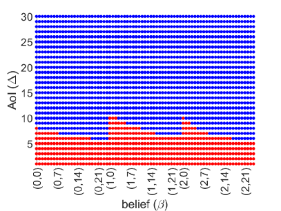
(a) $p=0.8$ and $\lambda=0.12$

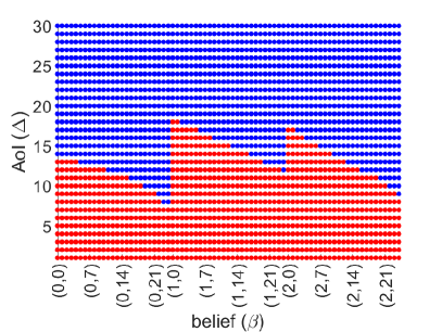
(b) $p=0.2$ and $\lambda=0.06$

Figure 4: Structure of an optimal policy $\pi^{*}(z)$ for each belief-state $z=(\beta,1,{\Delta})$.

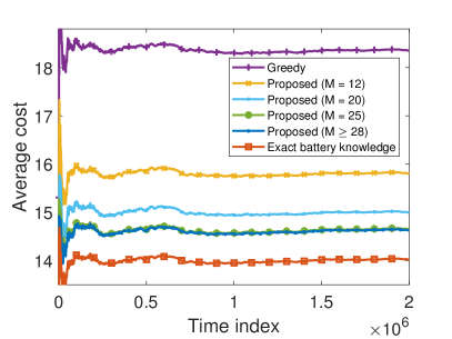
(a) $\lambda=0.04$

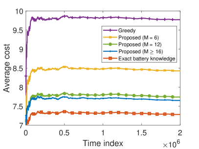
(b) $\lambda=0.08$

Figure 5: Performance of the proposed POMDP-based algorithm over time for single sensor scenario.

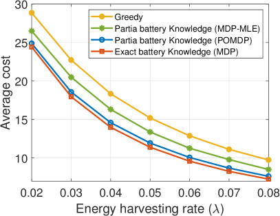
(a) $p=0.8$, $B=2$

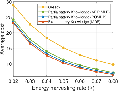
(b) $p=0.8$, $B=3$

Figure 6: Average cost with respect to the energy harvesting rate ($\lambda$) for single sensor scenario.

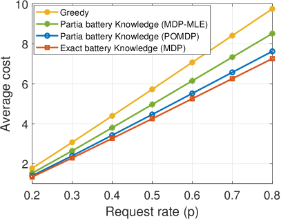
(a) $\lambda=0.08$, $B=2$

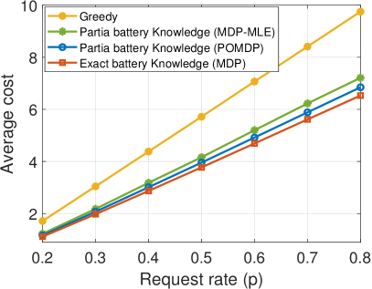
(b) $\lambda=0.08$, $B=3$

Figure 7: Average cost with respect to the request rate $p$ for single sensor setup.

V-A Single-sensor IoT Sensing Network

We consider a single-sensor scenario with $\lambda=0.06$, $p=0.8$, $\Delta^{\mathrm{max}}=64$, and $B=2$. Fig. 4 illustrates the structure of an optimal policy $\pi^{*}$, where each point represents a potential belief-state as a three-tuple $z=(\beta,r,{\Delta})$. For each such $z$, a blue point indicates that the optimal action is to command the sensor (i.e., $\pi^{*}(z)=1$), whereas a red point means not to command. Henceforth, we refer to the set of blue points as the command region. We use Table III-C to represent each belief on the x-axis of these figures; for example, $(0,5)$ is referred to the belief $\bm{\Lambda}^{5}\beta(1)$ and $(2,3)$ is referred to the belief $\bm{\Lambda}^{3}{\rho}^{2}$. As shown in Fig. 4(a), if there is no request (i.e., $r=0$), the optimal action is that the edge node does not command the sensor, regardless of the belief and AoI, i.e., $\pi^{*}(\beta,0,\Delta)=0$. In this case, the immediate cost (i.e., on-demand AoI (3)) becomes zero and the action $a(t)=0$ leads to energy saving for the sensor, which can be used later to serve the users with fresh measurements. Fig. 4 illustrates that $\pi^{*}$ has a threshold-based structure with respect to the AoI. To exemplify, consider the belief-state $z=((1,7),1,22)$ in which $\pi^{*}(z)=1$; then, by the threshold-based structure, $\pi^{*}(\underline{z})=1$ for all $\underline{z}=((1,7),1,\Delta)$, $\Delta\geq 20$. From Fig. 4, it can also be inferred that if the optimal action in belief-state $z=(\beta,1,\Delta)$ is $\pi^{*}(z)=1$, then the optimal action is $\pi^{*}(\underline{z})=1$ for all states $\underline{z}=(\bm{\Lambda}^{m}\beta,1,\Delta)$, $m=1,2,\dots$.

Comparing Fig. 4(b) and Fig. 4(a) reveals that the command region enlarges as the EH rate increases. This is because when a sensor harvests energy more frequently, it is able to transmit updates more frequently as well. By comparing Fig. 4(b) and Fig. 4(b), it is concluded that the command region shrinks as the request rate $p$ increases, because the edge node commands the sensor less to save its energy for the future requests.

Fig. 5 depicts the performance of the proposed algorithm over time. In the request-aware greedy policy, the edge node commands the sensor whenever there is a request (i.e., $r(t)=1$). As benchmark, we consider a case that the edge node knows the exact battery level at each time slot [5]. Clearly, this policy serves as a lower bound to the proposed POMDP-based algorithm. As shown in Fig. 5, for sufficiently large $M$ (e.g., $M\geq 28$ for $\lambda=0.04$ and $M\geq 16$ for $\lambda=0.08$), the proposed algorithm obtains optimal performance and reduces the average cost by approximately $25\leavevmode\nobreak\ \%$ compared to the greedy policy. Besides, the greater the value of $\lambda$, the smaller the value of $M$ for which the proposed algorithm attains optimal performance. This is because the power of the matrix $\Lambda$ converges faster. Furthermore, the performance of the proposed approach is not too far from the performance under the exact battery knowledge; this relatively small gap shows the impact of the uncertainty about the sensors’ battery levels.

Fig. 7 and Fig. 7 depict the average cost with respect to the energy harvesting rate $\lambda$ and the request rate $p$, respectively. As expected, the average cost decreases when $\lambda$ increases; the sensor harvests energy more often so that it can send fresh updates more often. Further, as the battery capacity $B$ increases, the performance of the MDP-based sub optimal policy (i.e., MLE) becomes closer to the optimal performance, and the gap between the optimal policy for partial battery case and the optimal policy for the exact battery knowledge decreases. Moreover, as shown in Fig. 7, the average cost increases as $p$ increases. This is because the command region shrinks as the sensor is requested more often.

V-B Multi-Sensor IoT Network

We consider a multi-sensor scenario where ${p_{k}=0.8}$, ${\Delta^{\mathrm{max}}=64}$, and ${B=3}$. Each sensor is assigned an energy harvesting rate $\lambda_{k}$ from the set $\{0.01,0.02,\dots,0.1\}$ sequentially: sensors ${1,11,\ldots}$ have the rate $0.01$, sensors ${2,12,\ldots}$ have the rate $0.02$, and so on. The following benchmarks are used for comparison. 1) A (request-aware) greedy policy where the edge node commands at most $N$ sensors with the largest AoI from the set $\mathcal{W}(t)\triangleq\{k\mid r_{k}(t)=1,k\in\mathcal{K}\}$, i.e., the set of sensors whose status are requested by a user, 2) The lower bound, obtained by following an optimal relaxed policy $\pi^{*}_{\mathrm{R}}$ (see (12) in [43]), and 3) the case where the edge node knows the exact battery levels at each slot for which the relax-then truncate approach is used to find an asymptotically optimal policy [6].

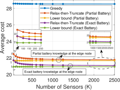
(a) $\Gamma=0.02$

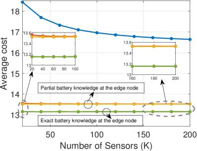
(b) $\Gamma=0.15$

Figure 8: Performance of the proposed relax-then-truncate approach in terms of average cost with respect to the number of sensors $K$ for multi-sensor setup under transmission constraint.

The performance of the relax-then-truncate algorithm concerning the number of sensors $K$ for various normalized transmission budget $\Gamma\triangleq\frac{N}{K}$ is shown in Fig. 8. The results were acquired by averaging each algorithm over $10$ episodes, each of length $10^{7}$ slots. First, the proposed algorithm achieves a reduction in the average cost of about $30\leavevmode\nobreak\ \%$ compared to the greedy policy. Due to asymptotic optimality of the proposed algorithm, the gap between the proposed policy and the lower bound is very small for large values of $K$; the same holds true for the exact battery knowledge. Interestingly, both relax-then-truncate approaches perform close to the optimal solutions even for moderate numbers of sensors. Moreover, Figs. 8(a) and (b) show that for large $\Gamma$, the proposed policy approaches the optimal performance for smaller values of $K$. The reason is that, as $\Gamma$ increases, the proportion of sensors that can be commanded at each slot increases, and thus, the proportion of truncated sensors (i.e., those not commanded under $\tilde{\pi}$ compared to $\pi^{*}_{\mathrm{R}}$) decreases.

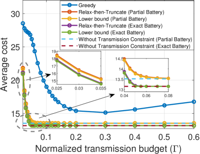
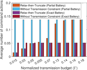
Figure 9: (a) Average cost and (b) Average number of command actions with respect to $\Gamma$ when ${K=1000}$ for multi-sensor setup under transmission constraint.

The average cost and average number of command actions with respect to the normalized transmission budget $\Gamma$ are illustrated in Fig. 9(a) and Fig. 9(b), respectively. For the benchmarking, we plot the performance of an optimal policy for the case with no transmission constraint (i.e., ${N\geq K}$) [5, 32]. As illustrated in Fig. 9(a), the average cost for the proposed algorithm decreases as $\Gamma$ increases. This is because, for a fixed $K$, increasing $\Gamma$ increases the transmission budget $N$, allowing the edge node to command more sensors at each slot and serve users with fresh status updates more frequently. Interestingly, there exists a point beyond which increasing $\Gamma$ does not lead to a decrease in the average cost. This is because, as depicted in Fig. 9(b), the average number of command actions ceases to increase (after ${\Gamma\geq 0.055}$ and ${\Gamma\geq 0.16}$ for exact and partial battery knowledge, respectively), meaning that the edge node has more transmission budget than required. In this case, the limited availability of the energy at the EH sensors becomes the primary constraint that limits the transmission of fresh status updates.

VI Conclusions

We investigated status updating under inexact knowledge about the battery levels of the energy harvesting (EH) sensors in an IoT network, where users make on-demand requests to a cache-enabled edge node to send status updates about various random processes monitored by the sensors. Accounting for the partial battery knowledge at the edge node, we derived a POMDP model for the on-demand AoI minimization problem. We converted the POMDP into a belief-state MDP and, via characterizing its key structures, developed an iterative algorithm that obtains an optimal policy for single sensor setup. Additionally, we proposed a sub-optimal MDP-based policy that has less computational complexity than the optimal POMDP-based policy. We also developed an efficient algorithm implementation leveraging the sparsity of the transition matrices. Furthermore, we extended our approach to the multi-sensor setup under a transmission constraint, where only a limited number of sensors can send status updates at each time slot. In particular, we developed a low-complexity relax-then-truncate algorithm and showed that it is asymptotically optimal as the number of sensors goes to infinity. Our numerical experiments showed that an optimal POMDP-based policy has a threshold-based structure, demonstrated the performance gains obtained by the proposed algorithm compared to a request-aware greedy policy, and depicted that the sub-optimal MDP-based method performs well when the battery capacity of the sensors increases. Furthermore, the performance of the proposed POMDP approach is not too far from the performance under the exact battery knowledge (acts as a lower bound); the relatively small gap shows the impact of the uncertainty about the sensors’ battery levels. Finally, our experiments illustrated that the relax-then-truncate method has near-optimal performance even for moderate numbers of sensors in the multi-sensor scenario under the transmission constraint.

-A Proof of Theorem 1

We start from the definition of the belief in (9) and express ${\beta_{j}(t+1)}$ as

$$\beta_{j}(t+1) =\Pr\left(b(t+1)=j\mid\phi^{\mathrm{c}}(t+1)\right)=\Pr\left(b(t+1)=j\mid\phi^{\mathrm{c}}(t),o(t+1),a(t)\right)$$ (27a)

$$=\frac{\Pr(b(t+1)=j,\phi^{\mathrm{c}}(t),o(t+1),a(t))}{\Pr(\phi^{\mathrm{c}}(t),o(t+1),a(t))}$$ (27b)

$$=\frac{\Pr(\phi^{\mathrm{c}}(t),a(t))\Pr(b(t+1)=j,o(t+1)\mid\phi^{\mathrm{c}}(t),a(t))}{\Pr(\phi^{\mathrm{c}}(t),a(t))\Pr(o(t+1)\mid\phi^{\mathrm{c}}(t),a(t))}$$ (27c)

$$=\frac{\Pr(b(t+1)=j,o(t+1)\mid\phi^{\mathrm{c}}(t),a(t))}{\Pr(o(t+1)\mid\phi^{\mathrm{c}}(t),a(t))}$$ (27d)

$$\overset{(a)}{=}\frac{\Pr(b(t+1)=j,o(t+1)\mid\phi^{\mathrm{c}}(t),a(t))}{\zeta}$$ (27e)

$$=\frac{1}{\zeta}\sum_{i=0}^{B}\Pr(b(t)=i,b(t+1)=j,o(t+1)\mid\phi^{\mathrm{c}}(t),a(t))$$ (27f)

$$=\frac{1}{\zeta}\sum_{i=0}^{B}\Bigg{[}\Pr(b(t)=i\mid\phi^{\mathrm{c}}(t),a(t))\Pr(b(t+1)=j\mid b(t)=i,\phi^{\mathrm{c}}(t),a(t))$$

$$\hskip 71.13188pt\Pr(o(t+1)\mid b(t+1)=j,b(t)=i,\phi^{\mathrm{c}}(t),a(t))\Bigg{]}$$ (27g)

$$\overset{(b)}{=}\frac{1}{\zeta}\sum_{i=0}^{B}\Bigg{[}\beta_{i}(t)\Pr(b(t+1)=j\mid b(t)=i,a(t))$$

$$\hskip 71.13188pt\Pr(o(t+1)\mid b(t+1)=j,b(t)=i,\phi^{\mathrm{c}}(t),a(t))\Bigg{]}$$ (27h)

where $(a)$ follows by introducing a normalization factor ${\zeta\triangleq\Pr(o(t+1)\mid\phi^{\mathrm{c}}(t),a(t))}$, which is calculated using ${\sum_{j}\beta_{j}(t+1)=1}$, and $(b)$ follows from i) $\Pr(b(t)=i\mid\phi^{\mathrm{c}}(t),a(t))=\Pr(b(t)=i\mid\phi^{\mathrm{c}}(t))$ because $b(t)$ is given when performing action $a(t)$, and subsequently using the belief definition $\beta_{i}(t)$ in (9), ii) $\Pr(b(t+1)=j\mid b(t)=i,\phi^{\mathrm{c}}(t),a(t))=\Pr(b(t+1)=j\mid b(t)=i,a(t))$ because $b(t+1)$ is independent of $\phi^{\mathrm{c}}(t)$ given $b(t)$ and $a(t)$. Next, we derive an expression for $\beta_{j}(t+1)$ in (27) for the different cases regarding action ${a(t)\in\{0,1\}}$.

-A1 Action $a(t)=0$

The edge node does not receive an update and thus the next observation is either $o(t+1)=(1,\min\{\Delta(t)+1,\Delta^{\mathrm{max}}\},\tilde{b}(t))$ or $o(t+1)=(0,\min\{\Delta(t)+1,\Delta^{\mathrm{max}}\},\tilde{b}(t))$, which happens with probability $p$ and $1-p$, respectively. Recall that $p$ is the probability of having a request at each slot (i.e., $\mathrm{Pr}\{r(t)=1\}=p$, $\forall t$). We next calculate the belief update function for $a(t)=0$ and $o(t+1)=(1,\min\{\Delta(t)+1,\Delta^{\mathrm{max}}\},\tilde{b}(t))$. By (27), we have

$$\beta_{j}(t+1) =\frac{1}{\zeta}\sum_{i=0}^{B}\Bigg{[}\beta_{i}(t)\Pr(b(t+1)=j\mid b(t)=i,a(t)=0)$$ (28)

$$\hskip 85.35826pt\underbrace{\Pr(o(t+1)\mid b(t+1)=j,b(t)=i,\phi^{\mathrm{c}}(t),a(t)=0)}_{\overset{(a)}{=}p}\Bigg{]}$$

$$=\frac{p}{\zeta}\sum_{i=0}^{B}\beta_{i}(t)\underbrace{\Pr(b(t+1)=j\mid b(t)=i,a(t)=0)}_{(\star)},$$

where $(a)$ follows from

$$\Pr\Bigg{(}o(t+1)=(1,\min\{\Delta(t)+1,\Delta^{\mathrm{max}}\},\tilde{b}(t))\mid b(t+1)=j,b(t)=i,$$

$$\hskip 85.35826pt\underbrace{(\phi^{\mathrm{c}}(t-1),r(t),\Delta(t),\tilde{b}(t),a(t-1))}_{\phi^{\mathrm{c}}(t)},a(t)=0\Bigg{)}=$$

$$\Pr\left(o(t+1)=(1,\min\{\Delta(t)+1,\Delta^{\mathrm{max}}\},\tilde{b}(t))\mid\Delta(t),\tilde{b}(t),a(t)=0\right){=}$$

$${\Pr\left(r(t+1)=1,\Delta(t+1)=\min\{\Delta(t)+1,\Delta^{\mathrm{max}}\},\tilde{b}(t+1)=\tilde{b}(t)\mid\Delta(t),\tilde{b}(t),a(t)=0\right)}\overset{(b)}{=}$$

$$\underbrace{\Pr(r(t+1)=1)}_{=p}\underbrace{\Pr(\Delta(t+1)=\min\{\Delta(t)+1,\Delta^{\mathrm{max}}\},\tilde{b}(t+1)=\tilde{b}(t)\mid\Delta(t),\tilde{b}(t),a(t)=0)}_{=1}$$

$$\hskip 14.22636pt=p,$$

where $(b)$ follows from the independence of the request process from the other variables. At each slot, the sensor harvests one unit of energy with probability $\lambda$. Thus, $(\star)$ in (28) is expressed as

$$\Pr(b(t+1)=j\mid b(t)=i<B,a(t)=0)=\left\{\begin{array}[]{ll}1-\lambda,&j=i,\\ \lambda,&j=i+1,\\ 0,&\mbox{otherwise.}\end{array}\right.$$ (29)

$$\Pr(b(t+1)=j\mid b(t)=B,a(t)=0)={\mathds{1}_{\{j=B\}}}.$$

By substituting (29) into (28), we can express $\beta_{j}(t+1)$, for each $j\in\{0,1,\ldots,B\}$, as

$$\begin{array}[]{ll}&\beta_{0}(t+1)=\frac{p}{\zeta}(1-\lambda)\beta_{0}(t),\\ &\beta_{1}(t+1)=\frac{p}{\zeta}(\lambda\beta_{0}(t)+(1-\lambda)\beta_{1}(t)),\\ &\dots,\\ &\beta_{B-1}(t+1)=\frac{p}{\zeta}(\lambda\beta_{B-2}(t)+(1-\lambda)\beta_{B-1}(t)),\\ &\beta_{B}(t+1)=\frac{p}{\zeta}(\lambda\beta_{B-1}(t)+\beta_{B}(t)).\end{array}$$ (30)

Using $\sum_{j=0}^{B}\beta_{j}(t+1)=1$, we can easily calculate the normalization factor to be ${\zeta=p}$. By rewriting (30) in the vector form, the updated belief is given by $\beta(t+1)=\bm{\Lambda}\beta(t)$, where the matrix $\bm{\Lambda}$ is defined in (11). For the case where $a(t)=0$ and ${o(t+1)=(0,\min\{\Delta(t)+1,\Delta^{\mathrm{max}}\},\tilde{b}(t))}$, one can follow the similar steps and conclude that ${\beta(t+1)=\bm{\Lambda}\beta(t)}$ as well.

-A2 Action $a(t)=1$

For the case where ${a(t)=1}$, the edge node receives an update whenever $b(t)\geq 1$ and does not receive an update if $b(t)=0$. In this regard, if ${b(t)=m\geq 1}$, the next observation is either $o(t+1)=(1,1,m)$ or $o(t+1)=(0,1,m)$, ${m\in\{1,2,\dots,B\}}$; and, if $b(t)=0$, the next observation is either $o(t+1)=(1,\min\{\Delta(t)+1,\Delta^{\mathrm{max}}\},\tilde{b}(t))$ or $o(t+1)=(0,\min\{\Delta(t)+1,\Delta^{\mathrm{max}}\},\tilde{b}(t))$. We next calculate the belief update function for these cases. Starting with $a(t)=1$ and ${o(t+1)=(1,\min\{\Delta(t)+1,\Delta^{\mathrm{max}}\},\tilde{b}(t)\})}$, by (27), we have

$$\beta_{j}(t+1) =\frac{1}{\zeta}\sum_{i=0}^{B}\Bigg{[}\beta_{i}(t)\Pr(b(t+1)=j\mid b(t)=i,a(t)=1)$$

$$\hskip 56.9055pt\Pr(o(t+1)\mid b(t+1)=j,b(t)=i,\phi^{\mathrm{c}}(t),a(t)=1)\Bigg{]}$$ (31a)

$$=\frac{1}{\zeta}\beta_{0}(t)\Pr(b(t+1)=j\mid b(t)=0,a(t)=1)$$

$$\hskip 56.9055pt\underbrace{\Pr(o(t+1)\mid b(t+1)=j,b(t)=0,\phi^{\mathrm{c}}(t),a(t)=1)}_{\overset{(a)}{=}p}$$

$$\hskip 28.45274pt+\frac{1}{\zeta}\sum_{i=1}^{B}\Bigg{[}\beta_{i}(t)\Pr(b(t+1)=j\mid b(t)=i,a(t)=1)$$

$$\hskip 56.9055pt\underbrace{\Pr(o(t+1)\mid b(t+1)=j,b(t)=i,\phi^{\mathrm{c}}(t),a(t)=1)}_{\overset{(b)}{=}0}\Bigg{]}$$ (31b)

$$=\frac{p\beta_{0}(t)}{\zeta}\Pr(b(t+1)=j\mid b(t)=0,a(t)=1)=\left\{\begin{array}[]{ll}\frac{p\beta_{0}(t)}{\zeta}(1-\lambda),&j=0,\\ \frac{p\beta_{0}(t)}{\zeta}\lambda,&j=1,\\ 0,&j=2,\ldots,B,\end{array}\right.$$ (31f)

where $(a)$ follows similarly as (-A1) and $(b)$ follows from

$$\begin{array}[]{ll}&\Pr\left(o(t+1)=(1,\min\{\Delta(t)+1,\Delta^{\mathrm{max}}\},\tilde{b}(t))\mid b(t+1)=j,b(t)=i\geq 1,\phi^{\mathrm{c}}(t),a(t)=1\right)\\ &=\Bigg{[}\Pr(r(t+1)=1)\\ &\underbrace{\Pr\!\left(\Delta(t+1)\!=\!\min\{\Delta(t)\!+\!1,\Delta^{\mathrm{max}}\},\tilde{b}(t+1)\!=\!\tilde{b}(t)\!\mid\!b(t+1)\!=\!j,b(t)\!=\!i\!\geq\!1,\!\phi^{\mathrm{c}}(t),a(t)\!=\!1\!\right)}_{\overset{(c)}{=}0}\Bigg{]}\\ &=0,\end{array}$$

where $(c)$ is because the edge node receives an update if $a(t)=1$ and $b(t)\geq 1$, and thus, $\Delta(t+1)=1$ (see (2)). Using $\sum_{j=0}^{B}\beta_{j}(t+1)=1$, we have ${\zeta=p\beta_{0}(t)}$. By rewriting (31) in the vector form, we have $\beta(t+1)={\rho}^{0}$ (see (12)). For $a(t)=1$ and $o(t+1)=(0,\min\{\Delta(t)+1,\Delta^{\mathrm{max}}\},\tilde{b}(t))$, one can follow the similar steps and conclude that $\beta(t+1)={\rho}^{0}$ as well.

For the cases where $a(t)=1$ and ${o(t+1)=(1,1,m)}$, $m\in\{1,2,\dots,B\}$, by (27), we have

$$\beta_{j}(t+1) =\frac{1}{\zeta}\sum_{i=0}^{B}\Bigg{[}\beta_{i}(t)\Pr(b(t+1)=j\mid b(t)=i,a(t)=1)$$ (32)

$$\hskip 99.58464pt\underbrace{\Pr(o(t+1)\mid b(t+1)=j,b(t)=i,\phi^{\mathrm{c}}(t),a(t)=1)}_{\overset{(a)}{=}p\mathds{1}_{\{i=m\}}}\Bigg{]}$$

$$=\frac{p\beta_{m}(t)}{\zeta}\Pr(b(t+1)=j\mid b(t)=m,a(t)=1)$$

$$=\left\{\begin{array}[]{ll}\frac{p\beta_{m}(t)}{\zeta}(1-\lambda),&j=m-1,\\ \frac{p\beta_{m}(t)}{\zeta}\lambda,&j=m,\\ 0,&\mbox{otherwise.}\end{array}\right.$$

where $\mathds{1}_{\{\cdot\}}$ is the indicator function and $(a)$ follows from

$$\Pr\big{(}o(t+1)=(1,1,m)\mid b(t+1)=j,b(t)=i,\phi^{\mathrm{c}}(t),a(t)=1\big{)}$$

$$=\Bigg{[}\underbrace{\Pr(r(t+1)=1)}_{=p}$$

$$\underbrace{\Pr\big{(}\Delta(t+1)=1,\tilde{b}(t+1)=m\geq 1\mid b(t+1)=j,b(t)=i,\phi^{\mathrm{c}}(t),a(t)=1\big{)}}_{\overset{(b)}{=}\mathds{1}_{\{i=m\}}}\Bigg{]}$$

$$=p\mathds{1}_{\{i=m\}},$$

where $(b)$ follows because the edge node receives an update whenever $a(t)=1$ and $b(t)\geq 1$, and thus, $\tilde{b}(t+1)=b(t)$ (see Section II-C). Using $\sum_{j=0}^{B}\beta_{j}(t+1)=1$, the normalization factor is derived as $\zeta=p\beta_{m}(t)$. Therefore, by (32), we have $\beta(t+1)={\rho}^{m}$, where the vectors ${\rho}^{m}$, $m\in\{1,2,\dots,B\}$, are defined in (12). For the cases where $a(t)=1$ and ${o(t+1)=(0,1,m)}$, $m\in\{1,2,\dots,B\}$, one can follow the similar steps and conclude that $\beta(t+1)={\rho}^{m}$.

-B Proof of Theorem 2

By rewriting the Bellman equation for the average cost POMDP [44, Chapter 7], we have

$$\bar{C}^{*}+h(z)=\min_{a\in\mathcal{A}}[c(z,a)+\sum_{o^{\prime}}\Pr(o^{\prime}\mid z,a)h(z^{\prime})],\leavevmode\nobreak\ z\in\mathcal{Z},$$

where $c(z,a)$ is the immediate cost obtained by choosing action $a$ in belief-state $z$, ${z=(\beta,o)=(\beta,r,\Delta,\tilde{b})}$ is the current belief state, ${o^{\prime}=(r^{\prime},\Delta^{\prime},\tilde{b}^{\prime})}$ is the observation given action $a$, and ${z^{\prime}=(\tau(\beta,o^{\prime},a),r^{\prime},\Delta^{\prime},\tilde{b}^{\prime})}$ is the next belief state given action $a$ and observation $o^{\prime}$. By defining an action-value function as $Q(z,a)\triangleq c(z,a)+\sum_{o^{\prime}}\Pr(o^{\prime}\mid z,a)h(z^{\prime})$, we have

$$Q(z,a) =c(z,a)+\sum_{o^{\prime}}\Pr(o^{\prime}\mid z,a)h(z^{\prime})$$ (33a)

$$=\sum_{s}\Pr(\underbrace{s}_{(b,s^{\mathrm{v}})}\mid z)c(s,a)+\sum_{o^{\prime}}\sum_{s}\underbrace{\Pr(o^{\prime},s\mid z,a)}_{\Pr(s\mid z,a)\Pr(o^{\prime}\mid s,z,a)}h(z^{\prime})$$ (33b)

$$=\sum_{b}\sum_{s^{\mathrm{v}}}\underbrace{\Pr(b,s^{\mathrm{v}}\mid\beta,o)}_{\mathds{1}_{\{s^{\mathrm{v}}=o\}}\Pr(b\mid\beta,s^{\mathrm{v}},o)}c(b,s^{\mathrm{v}},a)$$

$$\hskip 14.22636pt+\sum_{r^{\prime}}\sum_{\Delta^{\prime}}\sum_{\tilde{b}^{\prime}}\sum_{b}\sum_{s^{\mathrm{v}}}\underbrace{\Pr(b,s^{\mathrm{v}}\mid\beta,o,a)}_{\mathds{1}_{\{s^{\mathrm{v}}=o\}}\Pr(b\mid\beta,s^{\mathrm{v}},o,a)}\Pr(r^{\prime},\Delta^{\prime},\tilde{b}^{\prime}\mid b,s^{\mathrm{v}},\beta,o,a)h(z^{\prime})$$ (33c)

$$=\sum_{b}\beta_{b}c(b,o,a)+\sum_{r^{\prime}}\sum_{\Delta^{\prime}}\sum_{\tilde{b}^{\prime}}\sum_{b}\beta_{b}\Pr(r^{\prime},\Delta^{\prime},\tilde{b}^{\prime}\mid b,\underbrace{r,\Delta,\tilde{b}}_{o},a)h(z^{\prime})$$ (33d)

$$=\sum_{b}\beta_{b}c(b,o,a)+\sum_{b}\beta_{b}\sum_{r^{\prime}}\Pr(r^{\prime})\sum_{\Delta^{\prime}}\sum_{\tilde{b}^{\prime}}\Pr(\Delta^{\prime},\tilde{b}^{\prime}\mid b,\Delta,\tilde{b},a)h(z^{\prime}),$$ (33e)

where $s^{\mathrm{v}}=(r,\Delta,\tilde{b})$ is the visible part of the state, which is equivalent to the observation $o$ (i.e., $o=s^{\mathrm{v}}$). For the case where $a=0$, by Theorem 1, we have $z^{\prime}=(\tau(\beta,o^{\prime},0),r^{\prime},\Delta^{\prime},\tilde{b}^{\prime})={(\bm{\Lambda}\beta,r^{\prime},\min\{\Delta+1,\Delta^{\mathrm{max}}\},\tilde{b}^{\prime})}$, and thus, $Q(z=(\beta,r,\Delta,\tilde{b}),a=0)$ in (33) is expressed as

$$Q(z,0) =Q((\beta,r,\Delta,\tilde{b}),0)$$ (34a)

$$=\sum_{b}\beta_{b}\underbrace{c(b,r,\Delta,\tilde{b},a=0)}_{=r\min\{\Delta+1,\Delta^{\mathrm{max}}\}}+\sum_{b}\beta_{b}\sum_{r^{\prime}}\Pr(r^{\prime})\sum_{\Delta^{\prime}}\sum_{\tilde{b}^{\prime}}\underbrace{\Pr(\Delta^{\prime},\tilde{b}^{\prime}\mid b,\Delta,\tilde{b},a=0)}_{=\mathds{1}_{\{\Delta^{\prime}=\min\{\Delta+1,\Delta^{\mathrm{max}}\},\tilde{b}^{\prime}=\tilde{b}\}}}h(z^{\prime})$$ (34b)

$$=r\min\{\Delta+1,\Delta^{\mathrm{max}}\}\underbrace{\sum_{b}\beta_{b}}_{=1}$$

$$\hskip 28.45274pt+\sum_{r^{\prime}}\underbrace{[r^{\prime}p+(1-r^{\prime})(1-p)]}_{\Pr(r^{\prime})}h(\bm{\Lambda}\beta,r^{\prime},\min\{\Delta+1,\Delta^{\mathrm{max}}\},\tilde{b})\underbrace{\sum_{b}\beta_{b}}_{=1}$$ (34c)

$$=r\min\{\Delta+1,\Delta^{\mathrm{max}}\}+\sum_{r^{\prime}}[r^{\prime}p+(1-r^{\prime})(1-p)]h(\bm{\Lambda}\beta,r^{\prime},\min\{\Delta+1,\Delta^{\mathrm{max}}\},\tilde{b}).$$ (34d)

For the case where $a=1$, $Q(z=(\beta,r,\Delta,\tilde{b}),a=1)$ in (33) is expressed as

$$Q(z,1) =Q((\beta,r,\Delta,\tilde{b}),1)$$ (35a)

$$=\sum_{b=0}^{B}\beta_{b}c(b,r,\Delta,\tilde{b},a=1)+\sum_{b=0}^{B}\beta_{b}\sum_{r^{\prime}}\Pr(r^{\prime})\sum_{\Delta^{\prime}}\sum_{\tilde{b}^{\prime}}\Pr(\Delta^{\prime},\tilde{b}^{\prime}\mid b,\Delta,\tilde{b},a=1)h(z^{\prime})$$ (35b)

$$=\beta_{0}\underbrace{c(b=0,r,\Delta,\tilde{b},a)}_{=r\min\{\Delta+1,\Delta^{\mathrm{max}}\}}+\sum_{b=1}^{B}\beta_{b}\underbrace{c(b,r,\Delta,\tilde{b},a)}_{=r\times 1}$$

$$\hskip 28.45274pt+\beta_{0}\sum_{r^{\prime}}\Pr(r^{\prime})\sum_{\Delta^{\prime}}\sum_{\tilde{b}^{\prime}}\underbrace{\Pr(\Delta^{\prime},\tilde{b}^{\prime}\mid b=0,\Delta,\tilde{b},a)}_{=\mathds{1}_{\{\Delta^{\prime}=\min\{\Delta+1,\Delta^{\mathrm{max}}\},\tilde{b}^{\prime}=\tilde{b}\}}}h(z^{\prime})$$

$$\hskip 28.45274pt+\sum_{b=1}^{B}\beta_{b}\sum_{r^{\prime}}\Pr(r^{\prime})\sum_{\Delta^{\prime}}\sum_{\tilde{b}^{\prime}}\underbrace{\Pr(\Delta^{\prime},\tilde{b}^{\prime}\mid b,\Delta,\tilde{b},a=1)}_{=\mathds{1}_{\{\Delta^{\prime}=1,\tilde{b}^{\prime}=b\}}}h(z^{\prime})$$ (35c)

$$=r\beta_{0}\min\{\Delta+1,\Delta^{\mathrm{max}}\}+r\underbrace{\sum_{b=1}^{B}\beta_{b}}_{=1-\beta_{0}}+\Bigg{[}\beta_{0}\sum_{r\prime}[r^{\prime}p+(1-r^{\prime})(1-p)]$$

$$\hskip 56.9055pth(\underbrace{\tau(\beta,r^{\prime},\min\{\Delta+1,\Delta^{\mathrm{max}}\},\tilde{b},a=1)}_{\overset{(a)}{=}{\rho}^{0}},r^{\prime},\min\{\Delta+1,\Delta^{\mathrm{max}}\},\tilde{b})\Bigg{]}$$

$$\hskip 28.45274pt+\sum_{b=1}^{B}\beta_{b}\sum_{r^{\prime}}[r^{\prime}p+(1-r^{\prime})(1-p)]h(\underbrace{\tau(\beta,r^{\prime},1,b,a)}_{\overset{(a)}{=}{\rho}^{b}},r^{\prime},1,b)$$ (35d)

$$=r\beta_{0}\min\{\Delta+1,\Delta^{\mathrm{max}}\}+r(1-\beta_{0})$$

$$\hskip 28.45274pt+\beta_{0}\sum_{r^{\prime}=0}^{1}[r^{\prime}p+(1-r^{\prime})(1-p)]h({\rho}^{0},r^{\prime},\min\{\Delta+1,\Delta^{\mathrm{max}}\},\tilde{b})$$

$$\hskip 28.45274pt+\sum_{b=1}^{B}\beta_{b}\sum_{r^{\prime}=0}^{1}[r^{\prime}p+(1-r^{\prime})(1-p)]h({\rho}^{b},r^{\prime},1,b),$$ (35e)

where $(a)$ follows from Theorem 1.

-C Proof of Lemma 1

We prove this lemma by mathematical induction. For $m=1$, we have $\bm{\Lambda}$ as shown in (11), and hence, the lemma holds for $m=1$. Assume that the lemma holds for some $m$. We prove that the lemma also holds for $m+1$. We have

$$\begin{array}[]{ll}&\bm{\Lambda}^{m+1}=\bm{\Lambda}^{m}\bm{\Lambda}\\ =&\begin{pmatrix}(1-\lambda)^{m}&0&\cdots&0&0\\ m\lambda(1-\lambda)^{m-1}&(1-\lambda)^{m}&\cdots&0&0\\ \frac{m(m-1)}{2!}\lambda^{2}(1-\lambda)^{m-2}&m\lambda(1-\lambda)^{m-1}&\cdots&0&0\\ \frac{m(m-1)(m-2)}{3!}\lambda^{3}(1-\lambda)^{m-3}&\frac{m(m-1)}{2}\lambda^{2}(1-\lambda)^{m-2}&\cdots&0&0\\ \vdots&\vdots&\ddots&\vdots&\vdots\\ \lambda^{B-1}(1-\lambda)^{m-B+1}\prod_{\nu=0}^{B-2}\frac{(m-\nu)}{\nu+1}&\lambda^{B-2}(1-\lambda)^{m-B+2}\prod_{\nu=0}^{B-3}\frac{(m-\nu)}{\nu+1}&\cdots&(1-\lambda)^{m}&0\\ 1-\sum_{j^{\prime}=1}^{B}\Lambda_{j^{\prime},1}&1-\sum_{j^{\prime}=1}^{B}\Lambda_{j^{\prime},2}&\cdots&1-(1-\lambda)^{m}&1\end{pmatrix}\times\\ &\begin{pmatrix}1-\lambda&0&\cdots&0&0\\ \lambda&1-\lambda&\cdots&0&0\\ \vdots&\vdots&\ddots&\vdots&\vdots\\ 0&0&\cdots&1-\lambda&0\\ 0&0&\cdots&\lambda&1\end{pmatrix}\\ =&\begin{pmatrix}(1-\lambda)^{m+1}&0&\cdots&0&0\\ (m+1)\lambda(1-\lambda)^{m}&(1-\lambda)^{m+1}&\cdots&0&0\\ \frac{(m+1)m}{2!}\lambda^{2}(1-\lambda)^{m-1}&(m+1)\lambda(1-\lambda)^{m}&\cdots&0&0\\ \frac{(m+1)m(m-1)}{3!}\lambda^{3}(1-\lambda)^{m-2}&\frac{(m+1)m}{2}\lambda^{2}(1-\lambda)^{m-1}&\cdots&0&0\\ \vdots&\vdots&\ddots&\vdots&\vdots\\ \lambda^{B-1}(1-\lambda)^{m-B+2}\prod_{\nu=0}^{B-2}\frac{(m+1-\nu)}{\nu+1}&\lambda^{B-2}(1-\lambda)^{m-B+3}\prod_{\nu=0}^{B-3}\frac{(m-\nu+1)}{\nu+1}&\cdots&(1-\lambda)^{m+1}&0\\ 1-\sum_{j^{\prime}=1}^{B}\Lambda_{j^{\prime},1}&1-\sum_{j^{\prime}=1}^{B}\Lambda_{j^{\prime},2}&\cdots&1-(1-\lambda)^{m+1}&1\end{pmatrix}.\end{array}$$

-D Proof of Theorem 3

We consider two belief-states ${z=(\beta,r,\Delta,\tilde{b})}$ and ${\underline{z}=(\beta,r,\Delta,\underline{\tilde{b}})}$, where ${\tilde{b}\neq\underline{\tilde{b}}}$, and prove that $V(z)=V(\underline{z})$. As the sequence $\{V^{(i)}(z)\}_{{i=1,2,\ldots}}$ converges to $V(z)$ for any initialization, it suffices to prove that $V^{(i)}(\underline{z})=V^{(i)}(z)$, $\forall{i}$, which is established using mathematical induction. The initial values are selected arbitrarily, e.g., ${V^{(0)}(z)=0}$ and ${V^{(0)}(\underline{z})=0}$, and thus, $V^{(i)}(z)=V^{(i)}(\underline{z})$ holds for ${i=0}$. Now, suppose that $V^{(i)}(z)=V^{(i)}(\underline{z})$ for some $i$. Our goal is to prove that ${V^{(i+1)}(z)=V^{(i+1)}(\underline{z})}$ as well. Since, $V^{(i+1)}(z)=\min_{a}Q^{(i+1)}(z,a)$, $\forall z$, we prove that $Q^{(i+1)}(z,a)=Q^{(i+1)}(\underline{z},a)$, for all $a\in\{0,1\}$, which concludes the proof. We provide the proof for $a=0$; the proof follows similarly for $a=1$. For $a=0$, we have

$$Q^{(i+1)}(z,0)-Q^{(i+1)}(\underline{z},0)=\sum_{r^{\prime}=0}^{1}\Bigg{[}[r^{\prime}p+(1-r^{\prime})(1-p)]$$ (36)

$$\hskip 22.76219pt\underbrace{[V^{(i)}(\bm{\Lambda}\beta,r^{\prime},\min\{\Delta+1,\Delta^{\mathrm{max}}\},\tilde{b})-V^{(i)}(\bm{\Lambda}\beta,r^{\prime},\min\{\Delta+1,\Delta^{\mathrm{max}}\},\underline{\tilde{b}})]}_{\overset{(a)}{=}0}\Bigg{]}=0,$$

where step $(a)$ follows from the induction assumption.

-E Proof of Proposition 1

For any belief-state $z=(\beta,r,\Delta)$, action $a$, and next belief state $z^{\prime}=(\beta^{\prime},r^{\prime},\Delta^{\prime})$, we have

$$\Pr(z^{\prime}=(\beta^{\prime},r^{\prime},\Delta^{\prime})\mid z=(\beta,r,\Delta),a)=\sum_{i=0}^{B}\Bigg{[}\Pr(\beta^{\prime},r^{\prime},\Delta^{\prime},b=i\mid\beta,r,\Delta,a)=\Pr(r^{\prime})$$ (37)

$$\hskip 28.45274pt\sum_{i=0}^{B}\underbrace{\Pr(b=i\mid\beta,r,\Delta,a,r^{\prime})}_{=\beta_{i}}\Pr(\Delta^{\prime}\mid\beta,r,\Delta,b=i,a,r^{\prime})\Pr(\beta^{\prime}\mid\beta,r,\Delta,a,r^{\prime},\Delta^{\prime},b=i)\Bigg{]}.$$

For the case where $a=0$, we have

$$\Pr(z^{\prime}\mid z,a) =\Pr(r^{\prime})\sum_{i=0}^{B}\beta_{i}\underbrace{\Pr(\Delta^{\prime}\mid\beta,r,\Delta,b=i,a=0)}_{\overset{(a)}{=}\mathds{1}_{\{\Delta^{\prime}=\min\{\Delta+1,\Delta^{\mathrm{max}}\}\}}}\underbrace{\Pr(\beta^{\prime}\mid\beta,r,\Delta,a=0,r^{\prime},\Delta^{\prime},b=i)}_{\overset{(b)}{=}\mathds{1}_{\{\beta^{\prime}=\Lambda\beta\}}}$$ (38)

$$=\left\{\begin{array}[]{ll}(1-p),&\beta^{\prime}=\Lambda\beta,r^{\prime}=0,\Delta^{\prime}=\min\{\Delta+1,\Delta^{\mathrm{max}}\},\\ p,&\beta^{\prime}=\Lambda\beta,r^{\prime}=1,\Delta^{\prime}=\min\{\Delta+1,\Delta^{\mathrm{max}}\},\end{array}\right.$$

where $(a)$ is because the AoI increases by one given $a=0$, and $(b)$ follows from Theorem 1. Therefore, $\mathbf{P}^{0}$ has only two non-zero elements in each row, and consequently, ${\mathrm{nz}(\mathbf{P}^{0})=2|\mathcal{Z}|=4M(B+1)\Delta^{\mathrm{max}}}$. For the case where $a=1$, we have

$$\Pr(z^{\prime}\mid z,a) =\Pr(r^{\prime})\Bigg{[}\beta_{0}\underbrace{\Pr(\Delta^{\prime}\mid\beta,r,\Delta,b=0,a=1)}_{\overset{(a)}{=}\mathds{1}_{\{\Delta^{\prime}=\min\{\Delta+1,\Delta^{\mathrm{max}}\}\}}}\underbrace{\Pr(\beta^{\prime}\mid\beta,r,\Delta,a=0,r^{\prime},\Delta^{\prime},b=0)}_{\overset{(c)}{=}\mathds{1}_{\{\beta^{\prime}=\rho^{0}\}}}$$ (39)

$$\hskip 28.45274pt+\sum_{i=1}^{B}\beta_{i}\underbrace{\Pr(\Delta^{\prime}\mid\beta,r,\Delta,b=i,a=1)}_{\overset{(b)}{=}\mathds{1}_{\{\Delta^{\prime}=1\}}}\underbrace{\Pr(\beta^{\prime}\mid\beta,r,\Delta,a=0,r^{\prime},\Delta^{\prime},b=i)}_{\overset{(c)}{=}\mathds{1}_{\{\beta^{\prime}=\rho^{i}\}}}\Bigg{]}$$

$$=\left\{\begin{array}[]{ll}(1-p)\beta_{0};&\beta^{\prime}=\rho^{0},r^{\prime}=0,\Delta^{\prime}=\min\{\Delta+1,\Delta^{\mathrm{max}}\}\\ p\beta_{0};&\beta^{\prime}=\rho^{0},r^{\prime}=1,\Delta^{\prime}=\min\{\Delta+1,\Delta^{\mathrm{max}}\}\\ (1-p)\beta_{0};&\beta^{\prime}=\rho^{1},r^{\prime}=0,\Delta^{\prime}=1\\ p\beta_{1};&\beta^{\prime}=\rho^{1},r^{\prime}=1,\Delta^{\prime}=1\\ \vdots&\vdots\\ (1-p)\beta_{B};&\beta^{\prime}=\rho^{B},r^{\prime}=0,\Delta^{\prime}=1\\ p\beta_{B};&\beta^{\prime}=\rho^{B},r^{\prime}=1,\Delta^{\prime}=1\end{array}\right.$$

where $(a)$ is because the AoI increases by one given $b=0$, $(b)$ is because the AoI drops to one given $a=1$ and $b\geq 1$, and $(c)$ follows from Theorem 1. Thus, $\mathbf{P}^{1}$ has only $2(B+1)$ non-zero elements in each row, and consequently, $\mathrm{nz}(\mathbf{P}^{0})=2(B+1)|\mathcal{Z}|=4M(B+1)^{2}\Delta^{\mathrm{max}}$.

References

- [1] S. Kaul, R. Yates, and M. Gruteser, “Real-time status: How often should one update?” in Proc. IEEE Int. Conf. on Computer. Commun. (INFOCOM), Orlando, FL, USA, Mar. 25–30, 2012, pp. 2731–2735.
- [2] Y. Sun, I. Kadota, R. Talak, E. Modiano, and R. Srikant, “Age of information: A new metric for information freshness,” Synthesis Lectures on Communication Networks, vol. 12, no. 2, pp. 1–224, 2019.
- [3] M. Hatami, M. Jahandideh, M. Leinonen, and M. Codreanu, “Age-aware status update control for energy harvesting IoT sensors via reinforcement learning,” in Proc. IEEE Int. Symp. Pers., Indoor, Mobile Radio Commun., London, UK, Aug. 31–Sep. 3 2020.
- [4] M. Hatami, M. Leinonen, and M. Codreanu, “AoI minimization in status update control with energy harvesting sensors,” IEEE Trans. Commun., vol. 69, no. 12, pp. 8335–8351, Dec. 2021.
- [5] ——, “Minimizing average on-demand AoI in an IoT network with energy harvesting sensors,” in Proc. IEEE Works. on Sign. Proc. Adv. in Wirel. Comms., Lucca, Italy, Sep. 27–30, 2021, pp. 1–6.
- [6] M. Hatami, M. Leinonen, Z. Chen, N. Pappas, and M. Codreanu, “On-demand AoI minimization in resource-constrained cache-enabled IoT networks with energy harvesting sensors,” IEEE Trans. Commun., vol. 70, no. 11, pp. 7446–7463, Nov. 2022.
- [7] E. T. Ceran, D. Gündüz, and A. György, “Average age of information with hybrid ARQ under a resource constraint,” IEEE Trans. Wireless Commun., vol. 18, no. 3, pp. 1900–1913, Mar. 2019.
- [8] ——, “A reinforcement learning approach to age of information in multi-user networks with HARQ,” IEEE J. Sel. Areas Commun., vol. 39, no. 5, pp. 1412–1426, May 2021.
- [9] H. Tang, J. Wang, L. Song, and J. Song, “Minimizing age of information with power constraints: Multi-user opportunistic scheduling in multi-state time-varying channels,” IEEE J. Sel. Areas Commun., vol. 38, no. 5, pp. 854–868, May 2020.
- [10] I. Kadota, A. Sinha, E. Uysal-Biyikoglu, R. Singh, and E. Modiano, “Scheduling policies for minimizing age of information in broadcast wireless networks,” IEEE/ACM Trans. Netw., vol. 26, no. 6, pp. 2637–2650, Dec. 2018.
- [11] A. Maatouk, S. Kriouile, M. Assad, and A. Ephremides, “On the optimality of the Whittle’s index policy for minimizing the age of information,” IEEE Trans. Wireless Commun., vol. 20, no. 2, pp. 1263–1277, Feb. 2021.
- [12] S. Kriouile, M. Assaad, and A. Maatouk, “On the global optimality of Whittle’s index policy for minimizing the age of information,” IEEE Trans. Inf. Theory, vol. 68, no. 1, pp. 572–600, 2022.
- [13] Y. P. Hsu, E. Modiano, and L. Duan, “Scheduling algorithms for minimizing age of information in wireless broadcast networks with random arrivals,” IEEE Trans. Mobile Comput., vol. 19, no. 12, pp. 2903–2915, Dec. 2020.
- [14] A. Zakeri, M. Moltafet, M. Leinonen, and M. Codreanu, “Minimizing the aoi in resource-constrained multi-source relaying systems: Dynamic and learning-based scheduling,” IEEE Trans. Wireless Commun., pp. 1–1, 2023.
- [15] G. Yao, A. Bedewy, and N. B. Shroff, “Age-optimal low-power status update over time-correlated fading channel,” IEEE Transactions on Mobile Computing, pp. 1–1, 2022.
- [16] A. Gong, T. Zhang, H. Chen, and Y. Zhang, “Age-of-information-based scheduling in multiuser uplinks with stochastic arrivals: A POMDP approach,” in Proc. IEEE Global Telecommun. Conf., Taipei, Taiwan, Dec. 7–11, 2020, pp. 1–6.
- [17] Y. Shao, Q. Cao, S. C. Liew, and H. Chen, “Partially observable minimum-age scheduling: The greedy policy,” IEEE Trans. Commun., vol. 70, no. 1, pp. 404–418, Jan. 2022.
- [18] G. Stamatakis, N. Pappas, A. Fragkiadakis, and A. Traganitis, “Semantics-aware active fault detection in status updating systems,” arXiv preprint arXiv:2202.00923, 2022.
- [19] J. Liu, R. Zhang, A. Gong, and H. Chen, “Optimizing age of information in wireless uplink networks with partial observations,” IEEE Trans. Commun., vol. 71, no. 7, pp. 4105–4118, Jul. 2023.
- [20] S. S. Vilni, M. Moltafet, M. Leinonen, and M. Codreanu, “Multi-source AoI-constrained resource minimization under HARQ: Heterogeneous sampling processes,” IEEE Trans. Veh. Technol., pp. 1–15, 2023.
- [21] X. Wu, J. Yang, and J. Wu, “Optimal status update for age of information minimization with an energy harvesting source,” IEEE Trans. Green Commun. Netw., vol. 2, no. 1, pp. 193–204, Mar. 2018.
- [22] G. Stamatakis, N. Pappas, and A. Traganitis, “Control of status updates for energy harvesting devices that monitor processes with alarms,” in IEEE Globecom Workshops, Waikoloa, HI, USA, Dec. 9–13, 2019, pp. 1–6.
- [23] E. T. Ceran, D. Gündüz, and A. György, “Learning to minimize age of information over an unreliable channel with energy harvesting,” arXiv preprint arXiv:2106.16037, 2021.
- [24] C. Tunc and S. Panwar, “Optimal transmission policies for energy harvesting age of information systems with battery recovery,” in Proc. Annual Asilomar Conf. Signals, Syst., Comp., Pacific Grove, CA, USA, Nov. 3–6, 2019, pp. 2012–2016.
- [25] S. Leng and A. Yener, “Age of information minimization for an energy harvesting cognitive radio,” IEEE Trans. on Cogn. Commun. Netw., vol. 5, no. 2, pp. 427–439, May 2019.
- [26] E. Gindullina, L. Badia, and D. Gündüz, “Age-of-information with information source diversity in an energy harvesting system,” IEEE Trans. Green Commun. Netw., vol. 5, no. 3, pp. 1529–1540, Sep. 2021.
- [27] M. A. Abd-Elmagid, H. S. Dhillon, and N. Pappas, “A reinforcement learning framework for optimizing age of information in RF-powered communication systems,” IEEE Trans. Commun., vol. 68, no. 8, pp. 4747–4760, Aug. 2020.
- [28] ——, “AoI-optimal joint sampling and updating for wireless powered communication systems,” IEEE Trans. Veh. Technol., vol. 69, no. 11, pp. 14 110–14 115, Nov. 2020.
- [29] S. Leng and A. Yener, “Learning to transmit fresh information in energy harvesting networks,” IEEE Trans. Green Commun. Netw., vol. 6, no. 4, pp. 2032–2042, Dec. 2022.
- [30] A. Arafa, J. Yang, S. Ulukus, and H. V. Poor, “Timely status updating over erasure channels using an energy harvesting sensor: Single and multiple sources,” IEEE Trans. Green Commun. Netw., vol. 6, no. 1, pp. 6–19, Dec. 2022.
- [31] M. Hatami, M. Leinonen, Z. Chen, N. Pappas, and M. Codreanu, “Asymptotically optimal on-demand AoI minimization in energy harvesting IoT networks,” in Proc. IEEE Int. Symp. Inform. Theory, Espoo, Finland, Jun. 26–Jul. 1 2022, pp. 922–927.
- [32] M. Hatami, M. Leinonen, and M. Codreanu, “Status updating with an energy harvesting sensor under partial battery knowledge,” in Proc. IEEE Works. on Sign. Proc. Adv. in Wirel. Comms., Oulu, Finland, Jul. 4–6, 2022, pp. 1–5.
- [33] F. Chiariotti, J. Holm, A. E. Kalør, B. Soret, S. K. Jensen, T. B. Pedersen, and P. Popovski, “Query age of information: Freshness in pull-based communication,” IEEE Trans. Commun., vol. 70, no. 3, pp. 1606–1622, 2022.
- [34] F. Li, Y. Sang, Z. Liu, B. Li, H. Wu, and B. Ji, “Waiting but not aging: Optimizing information freshness under the pull model,” IEEE/ACM Trans. Netw., vol. 29, no. 1, pp. 465–478, Feb. 2021.
- [35] A. Baknina, O. Ozel, J. Yang, S. Ulukus, and A. Yener, “Sending information through status updates,” in Proc. IEEE Int. Symp. Inform. Theory, Vail, CO, USA, Jun. 17–22, 2018, pp. 2271–2275.
- [36] O. Sigaud and O. Buffet, Markov decision processes in artificial intelligence. John Wiley & Sons, 2013.
- [37] M. Araya-López, V. Thomas, O. Buffet, and F. Charpillet, “A closer look at MOMDPs,” in Proc. IEEE Int. Conf. Tools with Artificial Intelligence, Arras, France, Oct. 27–29, 2010, pp. 197–204.
- [38] M. L. Puterman, Markov decision processes: discrete stochastic dynamic programming. John Wiley & Sons, 2014.
- [39] J. N. Tsitsiklis, “NP-hardness of checking the unichain condition in average cost MDPs,” Operations Research Letters, vol. 35, no. 3, pp. 319–323, 2007.
- [40] S. Boyd, P. Diaconis, and L. Xiao, “Fastest mixing Markov chain on a graph,” SIAM review, vol. 46, no. 4, pp. 667–689, 2004.
- [41] S. Boyd, S. P. Boyd, and L. Vandenberghe, Convex optimization. Cambridge university press, 2004.
- [42] E. Altman, Constrained Markov decision processes. CRC Press, 1999, vol. 7.
- [43] M. Hatami, M. Leinonen, and M. Codreanu, “On the age-optimality of relax-then-truncate approach under partial battery knowledge in energy harvesting IoT networks,” arXiv preprint, 2022.
- [44] V. Krishnamurthy, Partially observed Markov decision processes. Cambridge university press, 2016.